hcm2010 chapter 10 freeway facilities - uspsites.poli.usp.br/d/ptr2377/hcm2010-freeval user guide...

HCM2010 Chapter 10

Freeway Facilities

User’s Guide to FREEVAL2010

Prepared by:

N. Rouphail, and B. Schroeder

Institute for Transportation Research & Education (ITRE)

Brian Eads, Crawford, Murphy and Tilly (CMT)

February 2011

Version History

February 27, 2011: Initial version released in conjunction with the publication of HCM 2010.

Computational Engine Disclaimer and Copyright

This material represents the computational engine implementation of the freeway facilities methodology

in Chapter 10 of the Highway Capacity Manual 2010.

This computational engine is offered as is, without warranty or promise of support of any kind either

expressed or implied. Under no circumstance will the National Academy of Sciences or the

Transportation Research Board (TRB) be liable for any loss or damage caused by the installation or use of

this product. The National Academy of Sciences, TRB, and the TRB National Cooperative Highway

Research Program (NVHRP) make no representation or warranty of any kind, expressed or implied, in

fact or in law, including without limitations the warranty of merchantability or the warranty of fitness for

a particular purpose, and shall not in any case be liable for any consequential or special damages.

This computational engine is subject to change without notice and does not represent a commitment on

the part of the National Academy of Sciences, the Committee on Highway Capacity and Quality of

Service, TRB, or the NCHRP to notify a person of such revisions.

This material and the copyrights therein are owned by the National Academies, NCHRP, and TRB.

Highway Capacity Manual 2010

FREEVAL-2010 User Guide Page i Contents February 2011

FREEVAL-2010 USER GUIDE

CONTENTS

1. INTRODUCTION ....................................................................................................... 1

Overview ................................................................................................................... 1

Chapter Organization .............................................................................................. 2

2. ENGINE STRUCTURE AND ORGANIZATION................................................. 3

Inputs ......................................................................................................................... 3

Outputs ...................................................................................................................... 3

3. STEP-BY-STEP INPUT CODING PROCEDURE ................................................. 4

Step A: Welcome Screen .......................................................................................... 4

Step B: Global Input Parameters ............................................................................. 5

Step C: Save File as a Different Name .................................................................... 5

Step D: Code Segment Types .................................................................................. 5

Step E: Segment Data Entry .................................................................................... 6

Step F: Weaving Data ............................................................................................... 7

Step G: Outputs ......................................................................................................... 8

Step H: Revising Input Data.................................................................................. 11

4. INTERPRETING OVERSATURATED RESULTS .............................................. 13


Contents Page ii FREEVAL-2010 User Guide February 2011

LIST OF EXHIBITS

Exhibit 1 FREEVAL-2010 Welcome Screen .................................................................. 4

Exhibit 2 Global Settings Dialog .................................................................................... 5

Exhibit 3 Save File Dialog ............................................................................................... 5

Exhibit 4 Defining Segment Types ................................................................................ 6

Exhibit 5 Data Input ........................................................................................................ 7

Exhibit 6 Weaving Dialog ............................................................................................... 8

Exhibit 7 Facility Summary Worksheet ........................................................................ 9

Exhibit 8 Time Interval Performance ............................................................................ 9

Exhibit 9 Output Graphs ............................................................................................... 10

Exhibit 10 LOS Summary Table ................................................................................... 10

Exhibit 11 Summary Output for Oversaturated Facility .......................................... 13

Exhibit 12 Oversaturated Output for Time Interval 3............................................... 14

Exhibit 13 Oversaturated Output for Time Interval 4............................................... 15

Exhibit 14 Graphical Output for Oversaturated Case ............................................... 16

Exhibit 15 LOS Summary Table for Oversaturated Scenario ................................... 16


FREEVAL-2010 User Guide Page 1 Introduction February 2011

1. INTRODUCTION

OVERVIEW

This document is intended to provide general guidance on the use of the

computational engine for HCM Chapter 10, Freeway Facilities. This document is

practitioner-friendly, not developer oriented. The focus is on how to use and

interpret the results of the computational engine. Detailed discussion on the

procedure itself along with engine documentation guidance for software

developers is provided in Chapter 25, Freeway Facilities: Supplemental.

The computational engine, FREEVAL (FREeway EVALuation) 2010 is a

computerized, worksheet-based environment designed to faithfully implement the

operational analysis computations for Undersaturated and Oversaturated

Directional Freeway Facilities. Thus, FREEVAL-2010 is a faithful implementation

of HCM Chapter 10, which incorporates all of the freeway segment procedures

outlined in Chapters 11, 12, and 13 for basic freeway segments, weaving

segments, and merge and diverge segments, respectively.

FREEVAL-2010 is executed in Microsoft Excel, with most computations

embedded in Visual Basic modules. The environment allows the user to analyze

a freeway facility of up to 70 analysis segments (to be defined) and for up to

twenty-four 15-min time intervals (6 h). The engine can generally handle any

facility that falls within these temporal and spatial constraints. However, it is

highly recommended that the total facility length not exceed 9–12 mi in length to

ensure consistency between demand variability over time and facility travel time.

Further, the analysis spatial and temporal boundaries (i.e. first and last time

intervals and first and last facility segments) should be uncongested and should

allow all queues to form and clear within the facility to assure that performance

measures fully account for the predicted extent of congestion and delay. These

aspects are discussed in detail in Chapter 10. In conformance with the 2010

HCM, all analyses are carried out using US customary units.

FREEVAL-2010 is organized as a sequence of linked Excel worksheets, and

can be used autonomously to analyze individual freeway segments or an entire

directional facility. The user must define the different freeway segments and

enters all necessary input data that are also required in the individual segment

chapters. These include segment length, number of lanes, length of acceleration

and deceleration lanes, heavy and recreational vehicle percentages, and the free-

flow speed. The latter can also be calculated in FREEVAL-2010 from the segment

or facility geometric attributes.

Consistent with Chapter 10, FREEVAL-2010 covers undersaturated and

oversaturated conditions. For oversaturated time intervals, traffic demands,

volume served and queues are tracked over time and space, as discussed in more

detail in Chapter 25. In addition to characterizing oversaturated conditions, the

most significant difference from the segment-based chapters is that FREEVAL

carries out all calculations using 15-min flow rates (expressed in vehicles per

hour). It therefore does not use a peak-hour factor (PHF). To replicate the example

problem results found in the segment chapters, PHF-adjusted flow rates must be


Introduction Page 2 FREEVAL-2010 User Guide February 2011

entered in FREEVAL directly. Heavy vehicle adjustments (using general terrain

factors or directly input for specific grade segments) are automatically handled

by the methodology.

The computational engine is further designed to allow the user to revise

input data following the completion of an analysis. This feature is intended to

perform quick sensitivity or “what if” analyses of different demand scenarios or

geometric changes to the facility. However, the user is cautioned to ensure that

all prior inputs are maintained when using FREEVAL for extensive scenario

evaluation. FREEVAL-2010 is not a commercial software product, and as such

relies on the voluntary commitment of the TRB Committee on Highway Capacity

and Quality of Service to address software bugs that may emerge in the course of

its use, and incorporate methodological changes over time.

CHAPTER ORGANIZATION

The next section gives a brief description of the FREEVAL-2010 structure and

organization. The document then presents a series of screenshots from the

computational engine, in a step-by-step –process description of input and output

requirements. The document concludes with a discussion on interpreting the

output for an oversaturated case, which is one of the major strengths and unique

attributes of the methodology.

The software user guidance in sections 3 and 4 is based on example problems

1 and 2 of Chapter 10 and the user is encouraged to reference that discussion for

further information on the interpretation of results.


FREEVAL-2010 User Guide Page 3 Engine Structure and Organization February 2011

2. ENGINE STRUCTURE AND ORGANIZATION

The FREEVAL computational engine is organized as a sequence of

computational worksheets; one for each 15-min time, or analysis period. These

worksheets are used both for data input and data output, with portions of the

worksheets that are irrelevant to a particular segment type automatically hidden

by the procedure. Additional worksheets are used for interim calculations and to

present facility summary statistics. Worksheets are hidden and write-protected

automatically as needed. A total of 24 time intervals can be included and up to 70

user-defined segments can be coded for a directional facility.

INPUTS

Data input in FREEVAL takes place in three locations.

First, a global input screen appears when first executing the methodology. It

contains basic settings for the number of time intervals and segments, as well as

global settings for free-flow speed and other facility-wide parameters.

Second, most inputs regarding individual segment geometry and volumes

appear in the individual time-period worksheets. Some variables are pre-coded with

default values, but can be readily overridden by user input. Also, many inputs

entered in time-period 1 are automatically copied to later time intervals. The user

must enter the demand flows for each mainline segment and for each ramp in

every time interval. These cells are highlighted in yellow in the engine to assist

with data entry.

The third and final set of inputs is related to the weaving segment

methodology. Due to the special data requirements for this methodology, inputs

are handled through a separate input dialog box that automatically appears when a

user codes a weaving segment and executes the analysis.

OUTPUTS

Data output in FREEVAL also appears in three places.

First, every time-period worksheet contains a summary of the measures of

effectiveness (MOEs) for each segment in that time interval. The worksheet also

contains facility average estimates of MOEs such as overall travel-time and

facility-average density, which is needed to estimate facility levels of service.

Second, a summary worksheet (labeled “Results Summary”) provides

overall segment performance across all time intervals.

The third type of output are 3-D contour plots and summary tables showing

how a select number of MOEs vary by segment and time interval such as

volume-to-capacity ratio, demand-to-capacity ratio, segment speed, segment

density, and level of service (LOS) (table only). All outputs are used to evaluate

the operational performance of a facility as will be described in section 4.

The next section provides a step-by-step outline of the input coding

procedure.


Step-by-Step input Coding Procedure Page 4 FREEVAL-2010 User Guide February 2011

3. STEP-BY-STEP INPUT CODING PROCEDURE

This section presents a detailed overview of the data input process in

FREEVAL through a series of screenshots. The engine is saved as an .xls file, but

can also be opened and executed in Excel 2007 and 2010. The computations are

performed using Visual Basic macros and macros must be enabled in order to

execute the spreadsheet.

STEP A: WELCOME SCREEN

After opening the program, a welcome screen appears (Exhibit 1). To begin

coding, the user clicks on the “Enter New Data” button in the center of the

screen. If macros are disabled, a security warning will appear at the top of the

screen (shown in Exhibit 1 for Office 2007). Select “Enable this content” in the

dialog box that appears.

Exhibit 1 FREEVAL-2010 Welcome

Screen


FREEVAL-2010 User Guide Page 5 Step-by-Step input Coding Procedure February 2011

STEP B: GLOBAL INPUT PARAMETERS

After selecting “Enter New Data” the global input dialog will appear (Exhibit

2). Here the user selects the number of time intervals and number of segments to

be analyzed. Other settings include whether the facility free-flow speed is known

or should be calculated, whether ramp metering is used, the type of terrain, and

the jam density of the facility (used for oversaturated calculations). After

completing all global settings, select “OK”. The macro will automatically delete

all extra worksheets for time intervals and unused columns for segments. Output

charts and tables are also updated. Depending on the computer used, this

process may take a few minutes.

STEP C: SAVE FILE AS A DIFFERENT NAME

A dialog box will prompt the user to save the file under a different name

(Exhibit 3). This step is of critical importance, since saving using the same name

will override the original macro and the code will be lost! In fact, it is strongly

recommend as a first step that the user creates at least one copy of the original

FREEVAL-2010 containing the code and keep it in safe storage.

STEP D: CODE SEGMENT TYPES

Next, the user enters the type of each segment (Exhibit 4). Note that the

number of columns has been reduced to match the number of segments defined

by the user. The proper way to define the appropriate number of segment is

explained in Chapter 10, including the requirement that the first and last

segments of the facility should be coded as basic segments. Also, the number of

Exhibit 2 Global Settings Dialog

Exhibit 3 Save File Dialog

The first and last segments of the modeled facility should be basic freeway segments.



input worksheets generated matches the number of (15-min) time intervals

selected in the global dialog box. Using drop-down menus, the user defines each

segment as a basic, on-ramp, off-ramp, weaving, or overlapping ramp segment

following HCM conventions (see Chapter 10). After identifying all segments,

click the “Segment Types Entered” button. After that action, the macro will

automatically black out all unneeded data entry cells. This process may take a

few minutes.

STEP E: SEGMENT DATA ENTRY

Next, the user enters all segment data for each time interval in sequence

(Exhibit 5). The common inputs needed for all segments are: length (ft), number

of lanes, free-flow speed (mi/h), segment demand (veh/h), % trucks, and % RVs.

Additionally, the user can utilize several adjustment factors that may affect the

operations of the facility. These will be discussed in a later section.

For all ramp and weaving segments, the user further needs to enter the ramp

demand flows and can adjust the heavy vehicle percentages as desired. Note that

a time interval corresponds to a 15-min period and as a result all volume inputs

should take the form of 15-min demand flow rates (in vehicles per hour). No

PHF adjustment is necessary.

After entering all input for one time interval, the user opens the tab for the

worksheet in the next time interval. For all subsequent time intervals, some

inputs are automatically copied from the t=1 worksheet. However, the engine

generally allows the user to override automatically generated input. Demand

volumes always need to be entered for all time intervals. After completing all

inputs for all time intervals and checking for correctness, click the “Run Entire

Analysis” button shown on the worksheet in the last time interval.

Exhibit 4 Defining Segment Types

All traffic data input need to be entered in the form of demand flow rates. The method internally tracks whether these demands are processed and distinguishes in the output between demand volumes (input) and the actual volume served (output).



STEP F: WEAVING DATA

If the analyst coded at least one weaving segment in the facility, a weaving

dialog box will appear after clicking “Run Entire Analysis” (Exhibit 6). The

dialog contains all needed input variables for the new HCM2010 weaving

methodology. Some variables are automatically passed through from the main

input worksheets, but can be edited by selecting any of the radio buttons in the

“Value Known” group. For example, weaving volumes in FREEVAL-2010 are

automatically estimated assuming a common exit percentage of on-ramp and

freeway mainline traffic onto the off-ramp. If the user has actual weaving counts,

these should be entered instead. After editing a value, it is important to click

“Update” first to ensure that the new data have been saved. Then click “OK”

when done.

For guidance on estimating the weaving-specific variables, the user is

referred to Chapter 11, Freeway Weaving Segments. Special attention should be

paid to the distinction between weaving segment length and the weaving short

length. In FREEVAL, the effective segment length is entered in the Excel

worksheets and is the length to which the calculated performance measures are

applied. However, the performance measures are calculated based on the short

length as discussed in Chapter 12. For example, a weaving segment may have a

short length of 1,500 ft, which is measured as the distances between the gores at

the on and off-ramps. Following the guidance given in Chapter 12, the

operational effects of the weaving segment often extend a distance of 500 ft

upstream and downstream of that short length. Consequently, the weaving

segment length should be entered as 2,500 ft in the time interval input

worksheets.

The user can select “Use defaults for all time intervals” to skip the detailed

data entry, but is required to enter data for each segment in the first time

interval. After entering all data for each time interval, click “OK”. If more than

one weaving segment exists or more than one time interval is used, the weaving

dialog will move to the next set of inputs.

Exhibit 5 Data Input

For weaving segments, the segment length is the length over which performance measures are applied. The performance measures are calculated using the short length, which is commonly shorter than the segment length.



To ensure that weaving segments are coded correctly, the reader is referred

to Chapter 12, where definitions for weaving segment short length, the number

of required lane changes, and the number of weaving lanes are provided. The

user should not accept the default values in the weaving dialog before consulting

Chapter 12 variable definitions and analysis conventions. The interchange

density is automatically calculated from the overall facility geometry, but can

also be user-adjusted. Since FREEVAL only know the number of ramps (and the

facility length), but not the number of interchanges, an average of two ramps per

interchange is assumed. Consequently, the interchange density is estimated as

half the total ramp density.

A default value for ramp-to-ramp flow is estimated as decribes above.

However, the user can adjust any of the values in the flow diagram and the

method will automatically calculate all remaining values when the user clicks the

"Update" button. A user adjustment for ramp-to-ramp flow is especially

important for two-sided weaves. This adjustment is selected using the radio

button at the top of the dialog. The weaving graphic shown in Exhibit 6

automatically changes when a two-sided weave is used.

STEP G: OUTPUTS

The summary worksheet labeled “Results Summary” (Exhibit 7) contains

aggregated results for all time intervals. It provides average speed and travel

time over all time intervals and gives the maximum demand-to-capacity ratio

(d/c) for each segment across all time intervals. Provided all segments operate

below capacity (at or below a d/c ratio of 1.00) in all time intervals, the facility

operations will be labeled as “globally undersaturated.” If that is the case, all

individual segment results are obtained by Chapter 11–13 methodologies. The

Exhibit 6 Weaving Dialog



aggregation of performance measures is consistent with the computations

presented in Chapters 10 and 25.

If any segment during any time interval operates at a d/c ratio > 1.0, the

facility is considered to be “oversaturated” and additional output is generated.

This is discussed in more detail below. From the summary worksheet, the user

can select any of the individual interval worksheets for detailed results (Exhibit

8). Additionally, a set of four summary graphs is created showing four key

MOEs over all segments and all time intervals (Exhibit 9).

From any of the time interval sheets (Exhibit 8) the user can select “revise

input data” to modify segment and time-interval specific data. However, the

user cannot add or delete segments or time intervals at this stage, since the

corresponding worksheets and columns have been customized in step B above.

No attempt is made to characterize facility LOS across multiple time intervals

Exhibit 7 Facility Summary Worksheet

Exhibit 8 Time Interval Performance



which may have very different operational performance and can therefore bias

the resulting facility LOS value considerably.

1

3

50.00

0.10

0.20

0.30

0.40

0.50

0.60

0.70

0.80

0.90

1.00

1 2 3 4 5 67

89

1011

Time Interval

d/c

Segment Number

d/c Contours

0.90-1.00

0.80-0.90

0.70-0.80

0.60-0.70

0.50-0.60

0.40-0.50

0.30-0.40

0.20-0.30

0.10-0.20

0.00-0.10

1

3

50.00

0.10

0.20

0.30

0.40

0.50

0.60

0.70

0.80

0.90

1.00

1 2 3 4 5 67

89

1011

Time Interval

v/c

Segment Number

v/c Contours

0.90-1.00

0.80-0.90

0.70-0.80

0.60-0.70

0.50-0.60

0.40-0.50

0.30-0.40

0.20-0.30

0.10-0.20

0.00-0.10

1

3

50.00

10.00

20.00

30.00

40.00

50.00

60.00

1 2 3 4 5 6 7 89

1011

Time Interval

Spe

ed

(mi/

hr)

Segment Number

Space Mean Speed Contours (mi/hr)

50.00-60.00

40.00-50.00

30.00-40.00

20.00-30.00

10.00-20.00

0.00-10.00

1

3

50.00

5.00

10.00

15.00

20.00

25.00

30.00

35.00

40.00

45.00

1 2 3 4 5 6 7 89

1011

Time Interval

De

nsi

ty (

veh

/mi/

ln)

Segment Number

Density Contours (veh/mi/ln)

40.00-45.00

35.00-40.00

30.00-35.00

25.00-30.00

20.00-25.00

15.00-20.00

10.00-15.00

5.00-10.00

0.00-5.00

The four graphs in Exhibit 9 show performance measures over the time-

space domain. The v/c and d/c graphs in this case are identical, because the

facility is globally undersaturated. The speed plot shows a slight reduction in

speed in the weaving segment (segment 6) resulting from relatively high

weaving volumes that still do not exceed capacity. The density plot shows

elevated densities in segments 8 and 9. Note that the length axis in the graphs is

categorical and the scale therefore does not reflect the different lengths of

segments.

In addition to the graphical outputs, FREEVAL also gives summary tables of

the same four performance measures (v/c, d/c, speed, and density), as well as

LOS. Exhibit 10 shows only the LOS table, since other outputs are already

represented in the previous exhibit.

Exhibit 9 Output Graphs

Exhibit 10 LOS Summary Table



Consistent with the discussion in Chapter 10, FREEVAL provides two LOS

summary tables. The upper table in Exhibit 10 gives the density-based levels of

service criteria, which in this case are all at LOS E or better. The bottom table

gives supplemental LOS information for any segments where demand exceeds

capacity. Since all segments operate below capacity, no entries are shown in the

demand-based LOS table.

STEP H: REVISING INPUT DATA

Step G above concludes the freeway facility methodology outlined in

Chapter 10. It is expected, however, that analysts will use the methodology to

test various scenarios or to perform sensitivity analyses. The FREEVAL

computational engine has been designed to allow the user to revise input data

and make changes to geometry, demand patterns or other input variables to test

the effect of such changes on the operations of the facility. Motivations to revise

inputs include:

Testing sensitivity of increased volumes due to traffic growth or traffic

diversion to other routes;

Testing geometric changes such as added lanes, different ramp

configurations, or alternate weaving patterns in select segments; and

Testing the operational effects of work zones and/or incidents through

changes in segment capacity and/or free-flow speeds.

As stated earlier, the input revision does not allow the analyst to change the

number of segments or time intervals. This limitation is due to the manner in

which the engine customizes the segment columns and time interval worksheets

in step B. If the analyst wishes to modify the temporal or spatial analysis domain,

the facility has to be re-coded.

FREEVAL provides two types of adjustment factors that are intended to

assist the user in performing basic sensitivity analyses. These are:

Origin/Destination Demand Adjustment Factors, and

Capacity Adjustment Factors.

The two adjustment factors are described in more detail below.

Origin/Destination Demand Adjustment Factors

The origin and destination demand adjustment factors are used to test the

effect of an increase or decrease in the original demand volumes by a user-

defined growth or shrinkage factor. Each segment contains one origin and one

destination adjustment factor for each time interval. They act as simple

multiplicative factors that adjust the entering and exiting demands in the

segment. For example, an origin adjustment factor of 1.10 increases the demand

of mainline or an on-ramp segment by 10%. Similarly, a destination adjustment

factor of 0.85 will reduce the demand at an off-ramp by 15%. For weaving

segments, the entering and exiting demands can be changed with the applicable

origin and destination adjustment factors, respectively.



The origin/destination demand adjustment factors are intended to run quick

sensitivity analyses or what-if analyses of demand scenarios. For example, they

can be used to quickly assess the impact of ITS treatments that cause a

proportion of drivers to leave the freeway at an off-ramp upstream of a freeway

bottleneck. Similarly, they could be used to model a surge in on-ramp traffic. The

analyst can change all origin and destination demand adjustment factors by the

same value to model general background traffic growth (e.g. 1.05 for 5% traffic

growth).

Capacity Adjustment Factors

The capacity adjustment factors (CAF) are used to decrease the capacity of a

segment in one or more time intervals. The HCM capacity value for the segment

in the selected time interval is multiplied by the CAF. As a result, the speed-flow

relationship on the segment is changed as is discussed in more detail in Chapters

10 and 25. Capacity adjustment factors can be used to model short-term incidents

in a segment or to represent the effects of increased friction due to work zones, or

simply to calibrate the basic capacity to an observed, non-HCM condition (e.g.,

freeway tunnel). Capacity adjustment factors should generally only be used to

reduce the per-lane capacity in a segment. The speed-flow and capacity

relationships in Chapters 10–13 have been calibrated and an adjustment to higher

capacities (e.g. greater than 2,400 veh/h/ln) is not supported by the data. From a

computational perspective, the equation used to calculate the new speed-flow

relationship after applying a CAF, can further result in speeds above the free-

flow if a CAF>1.0 is used. If the user wishes to use the CAF to calibrate

FREEVAL-2010 to higher field-observed speeds, a higher free-flow speed curve

should be used. This speed-flow curve can then be calibrated to a lower capacity

using the CAF if desired.

The effect of advanced traffic management strategies, such as temporary

shoulder use, should be modeled by adding a lane in the appropriate segments

and time intervals, and then reducing the capacity of the revised segment using a

capacity adjustment factor (since the use of a shoulder is unlikely to result in a

full lane of added capacity. For example, if the use of the shoulder on a 3-lane, 70

mi/h basic freeway segment (per-lane capacity of 2,400 veh/h/ln) results in an

additional half-lane of capacity (1,200 veh/h/ln), it should be modeled as a four-

lane segment with a capacity adjustment factor of 0.875 (=[3 × 2,400 + 1,200] / [4 ×

2,400]).

Capacity adjustment factors should generally only be used to reduce the per-lane capacity in a segment, not to increase capacity above the calibrated HCM2010 capacity for that segment type.


FREEVAL-2010 User Guide Page 13 Interpreting Oversaturated Results February 2011

4. INTERPRETING OVERSATURATED RESULTS

This section discusses the interpretation of results for an oversaturated

freeway facility. A freeway facility is defined as oversaturated if any segment

experiences a d/c ratio greater than 1.0 during any analysis time interval. In the

facility summary worksheet, this facility will be labeled as “oversaturated” as

shown in Exhibit 11. If this is the case, the user should first ensure that whatever

queues that have formed during the analysis have dissipated by the end of the

last time interval and that all vehicles were able to clear the facility. To check for

this, the total vehicle-miles-traveled (VMT) based on demand flow (VMTD)

should exactly match the actual VMT processed (VMTV) in the Results Summary

worksheet. If these two numbers match (within a rounding margin of error), a

message appears indicating that “All Vehicles have cleared within the analysis

period.” If not, the analysis violates the underlying assumptions of Chapter 10,

which requires that all queues should be fully contained within the time-space

domain. If VMT-Demand does not equal VMT-Volume, this assumption is

violated in the time-dimension.

If a violation in the space-dimension occurs, an additional warning message

will alert the user that “The queue in time interval X extends beyond the analysis

region.” In either case, the analyst should start over and re-run the analysis with

additional segments and/or time intervals as appropriate. An alternative in the

case of space-dimension violation is to artificially increase the length of the first

upstream segment until the spillover queue is captured within the facility

confines. A congested boundary of the time-space domain means that vehicles

either remain on the facility by the end of the analysis, or in the case of extended

queuing upstream of the first segment, that the impact is not accounted for in the

delay and travel times computed for the facility. Only if all boundaries of the

time-space domain are free of queuing, can it be assured that FREEVAL-2010

represents the true extent of congestion.

The oversaturated facility shown in Exhibit 11 was generated by applying

across-the-board origin/destination demand adjustment factors of 1.11 to all

segments and time intervals for the undersaturated facility presented above. This

represents an 11% overall growth in traffic flow.

Only if all boundaries of the time-space domain are free of queuing, can it be assured that FREEVAL-2010 represents the true extent of congestion.

Exhibit 11 Summary Output for Oversaturated Facility


Interpreting Oversaturated Results Page 14 FREEVAL-2010 User Guide February 2011

The summary output in Exhibit 11 gives insight on congestion patterns and

severity. In the example, a total of 4 segments are shown to have a maximum d/c

ratio greater than 1.0 (segments 8, 9, 10, and 11). Segments 5, 6, and 7 all have

queuing starting in time interval 3, suggesting an active bottleneck in segment 8.

The downstream segments 9 and 10 are not exhibiting a queue, suggesting that

demand is metered at the segment 8 bottleneck. The d/c ratios greater than 1.0

without any associated queuing indicate hidden bottlenecks.

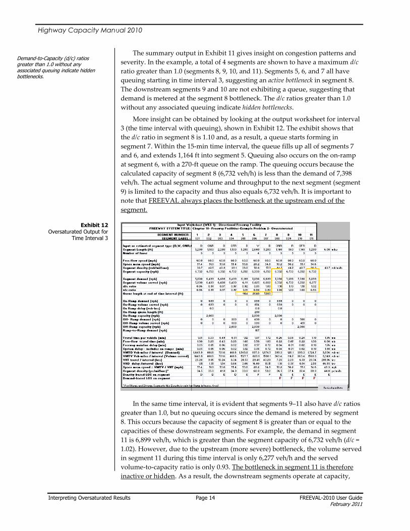
More insight can be obtained by looking at the output worksheet for interval

3 (the time interval with queuing), shown in Exhibit 12. The exhibit shows that

the d/c ratio in segment 8 is 1.10 and, as a result, a queue starts forming in

segment 7. Within the 15-min time interval, the queue fills up all of segments 7

and 6, and extends 1,164 ft into segment 5. Queuing also occurs on the on-ramp

at segment 6, with a 270-ft queue on the ramp. The queuing occurs because the

calculated capacity of segment 8 (6,732 veh/h) is less than the demand of 7,398

veh/h. The actual segment volume and throughput to the next segment (segment

9) is limited to the capacity and thus also equals 6,732 veh/h. It is important to

note that FREEVAL always places the bottleneck at the upstream end of the

segment.

In the same time interval, it is evident that segments 9–11 also have d/c ratios

greater than 1.0, but no queuing occurs since the demand is metered by segment

8. This occurs because the capacity of segment 8 is greater than or equal to the

capacities of these downstream segments. For example, the demand in segment

11 is 6,899 veh/h, which is greater than the segment capacity of 6,732 veh/h (d/c =

1.02). However, due to the upstream (more severe) bottleneck, the volume served

in segment 11 during this time interval is only 6,277 veh/h and the served

volume-to-capacity ratio is only 0.93. The bottleneck in segment 11 is therefore

inactive or hidden. As a result, the downstream segments operate at capacity,

Demand-to-Capacity (d/c) ratios greater than 1.0 without any associated queuing indicate hidden bottlenecks.

Exhibit 12 Oversaturated Output for

Time Interval 3


FREEVAL-2010 User Guide Page 15 Interpreting Oversaturated Results February 2011

which is defined as density-based LOS E. The fact that these segments do have

d/c ratios greater than 1.0 is reflected in the demand-based LOS, which is LOS F

for segments 9 through 11. This recognizes that the segment would fail if the

upstream bottleneck did not exist (or was alleviated through geometric changes

to the facility at that location only).

The results for time interval 3 in Exhibit 12 show that not all the forecasted

demand actually reaches segment 9–11, due to congestion in segment 8. Because

some vehicles were not served in time interval 3, they are now added as residual

demand in time interval 4. Exhibit 13 shows this effect. While the segment 9–11

served volumes were lower than the demand in time interval 3, the volumes are

greater than the demand in time interval 4. For example, segment 11 demand is

5,500 veh/h, but as the upstream queue clears, the actual served volume is 6,121

veh/h in this time interval. The output further shows that due to a drop in

demand from time intervals 3 to 4, all queues have cleared at the end of the 15-

min interval.

The effects of congestion are also evident in the graphical output provided as

part of FREEVAL. The graphs in Exhibit 14 are the same as already introduced in

Exhibit 9, but now show the effect of congestion. Most importantly, while the

under-saturated d/c and v/c graphs in Exhibit 9 were identical, the oversaturated

v/c graph limits the throughput of the active bottleneck in segment 8 to 1.0. It

further shows the metering effect in segments 9 through 11. The speed graph

shows a significant drop in speed as a result of the active bottleneck, but further

shows that operating conditions downstream of segment 8 are acceptable. This

point is critical, since an individual segment analysis of segments 9–11 would

have predicted a much lower and congested speed. The density plot further

shows areas of queuing with densities exceeding 45 veh/mi/ln in the queued

segments.

Exhibit 13 Oversaturated Output for Time Interval 4


Interpreting Oversaturated Results Page 16 FREEVAL-2010 User Guide February 2011

1

3

50.00

0.20

0.40

0.60

0.80

1.00

1.20

1 2 3 4 5 67

89

1011

Time Interval

d/c

Segment Number

d/c Contours

1.00-1.20

0.80-1.00

0.60-0.80

0.40-0.60

0.20-0.40

0.00-0.20

1

3

50.00

0.20

0.40

0.60

0.80

1.00

1.20

1 2 3 4 5 67

89

1011

Time Interval

v/c

Segment Number

v/c Contours

1.00-1.20

0.80-1.00

0.60-0.80

0.40-0.60

0.20-0.40

0.00-0.20

1

3

50.00

10.00

20.00

30.00

40.00

50.00

60.00

1 2 3 4 5 6 7 89

1011

Time Interval

Spe

ed

(mi/

hr)

Segment Number

Space Mean Speed Contours (mi/hr)

50.00-60.00

40.00-50.00

30.00-40.00

20.00-30.00

10.00-20.00

0.00-10.00

1

3

50.00

10.00

20.00

30.00

40.00

50.00

60.00

1 2 3 4 5 6 7 89

1011

Time Interval

De

nsi

ty (

veh

/mi/

ln)

Segment Number

Density Contours (veh/mi/ln)

50.00-60.00

40.00-50.00

30.00-40.00

20.00-30.00

10.00-20.00

0.00-10.00

The LOS summary table for the oversaturated scenario now clearly shows

the distinction between the density-based LOS that uses the actual volumes

served on the facility and the demand-based LOS table that shows the presence

of all segments with d/c ratios greater than 1.0, including all active and hidden

bottlenecks (Exhibit 15).

The density-based LOS table in Exhibit 15 shows that segments 6 and 7

operate at LOS F in time interval 3. In this case, Segment 8 is the active bottleneck

and because FREEVAL places the bottleneck at the beginning of the segment, it

operates at capacity, or LOS E. Since all downstream segments have capacities

less than or equal to that of the active bottleneck, they also operate at LOS E. The

bottom portion of Exhibit 15 shows the demand-based LOS, which emphasizes

that segments 8–11 all have d/c ratios greater than 1.0 in time interval 3. The

comparison between the density-based and demand-based LOS tables allows a

quick and easy analysis of which bottlenecks are active and which segments are

inactive or hidden bottlenecks due to an upstream metering effect of traffic

demand. The overall facility LOS is F in time interval 3, since one or more

individual segments have d/c ratios greater than 1.0.

Exhibit 14 Graphical Output for Oversaturated Case

Exhibit 15 LOS Summary Table for Oversaturated Scenario

hcm2010 chapter 10 freeway facilities - uspsites.poli.usp.br/d/ptr2377/hcm2010-freeval user guide...

Documents