hcsea2009 benefits of selfdiagnosingusms en 2009-03

8th South East Asia Hydrocarbon Flow Measurement Workshop4th – 6th March 2009

THE BENEFITS OF A FULLY SELF DIAGNOSINGGAS ULTRASONIC METERMr. John Lansing, SICK, Houston, Texas

Mr. Koos van Helden, SICK Engineering GmbH, GermanyDr. Volker Herrmann, SICK Engineering GmbH, Germany

1. ABSTRACT

During the past several years the use of ultrasonic meters (USMs) has gained world-wideacceptance for fiscal applications. The many benefits of USMs have been documented in papersat virtually every major conference. As the cost of gas continues to increase, the significance ofknowing that the ultrasonic meter is operating accurately has never been more important. The useof diagnostics to help identify metering issues has been discussed in several papers over the pastfew years [Ref 1, 2 & 12].

The traditional method of verifying whether the USM is operating accurately essentially requiresusing the USMs’ diagnostic information to help understand the meter’s health. This has oftenbeen referred to as Conditioned Based Maintenance, or CBM for short. Different USM meterdesigns require different analysis techniques, especially for the velocity profile analysis. For thefield technician, it is often difficult to understand all the diagnostic features of each USM meterdesign. Through the years software has been developed to help determine if the meter isoperating correctly or not. However, it is still very difficult to clearly define limits on some of thediagnostic parameters that translate into a quantifiable metering error.

This paper will discuss two methods of providing a fully redundant self diagnosing meter. The firstis a new CBM concept to assist in determining if the fiscal 4-path USM meter is operatingaccurately. Rather than relying entirely on the understanding and interpretation of the meter’sdiagnostics, a meter designed with an additional built-in diagnostic path, has been developed. Inthis paper the meter design will be referred to as the CBM 2Plex 4+1 meter.

The second is having a meter which monitors, on a real-time basis, all diagnostic parameters andthen reports when one, or more, approach unacceptable values. Traditionally in the past the userwould collect log files monthly and analyze them. The problem is that often the technician wouldoverlook a problem and thus it could develop into a significant measurement error. Also, sinceinspections are often performed on a monthly basis, a problem can develop and it may take amonth or more before the user would see this. By monitoring the diagnostics on a real-time basis,combined with the redundancy of an independent, second metering path of the CBM 2Plex 4+1meter, all aspects of a “meter’s health” can be checked and validated without the need formonthly inspections. This not only significantly reduces operation and maintenance (O&M)expenditures, but lowers measurement uncertainty in the field.

2. INTRODUCTION

The first part of this system starts with a CBM 2Plex 4+1 meter design which is a conventionalfiscal 4-path chordal ultrasonic meter that incorporates an additional, independent single-pathmeter and associated electronics incorporated into the same body. The purpose of the additionalpath is for continuous comparison of volumes to the fiscal 4-path meter’s measurement results.

The transducers for the independent single path are located in such a fashion as to traverse themeter in the center of the meter body. The transducers for the fiscal 4-path meter are located inthe traditional Westinghouse configuration. The reason for locating the single-path in the middle(center vertically) is to put it in the most profile-sensitive measurement position of the meter. Thiswill result in a difference in volumes between the single path and the fiscal 4-path when thevelocity profile changes. That is, the single-path meter, with the sensors located in the center ofthe flowing gas, is more sensitive to flow disturbances than the 4-path meter design.

These disturbances (velocity profile changes) can be caused by several external factors includingpartially blocked flow conditioners and pipeline contamination. All of these will cause a change inthe velocity profile seen at the meter. This concept works because changes in profiles significantlyimpact the reading by the centrally located single path while having very little affect on the 4-path


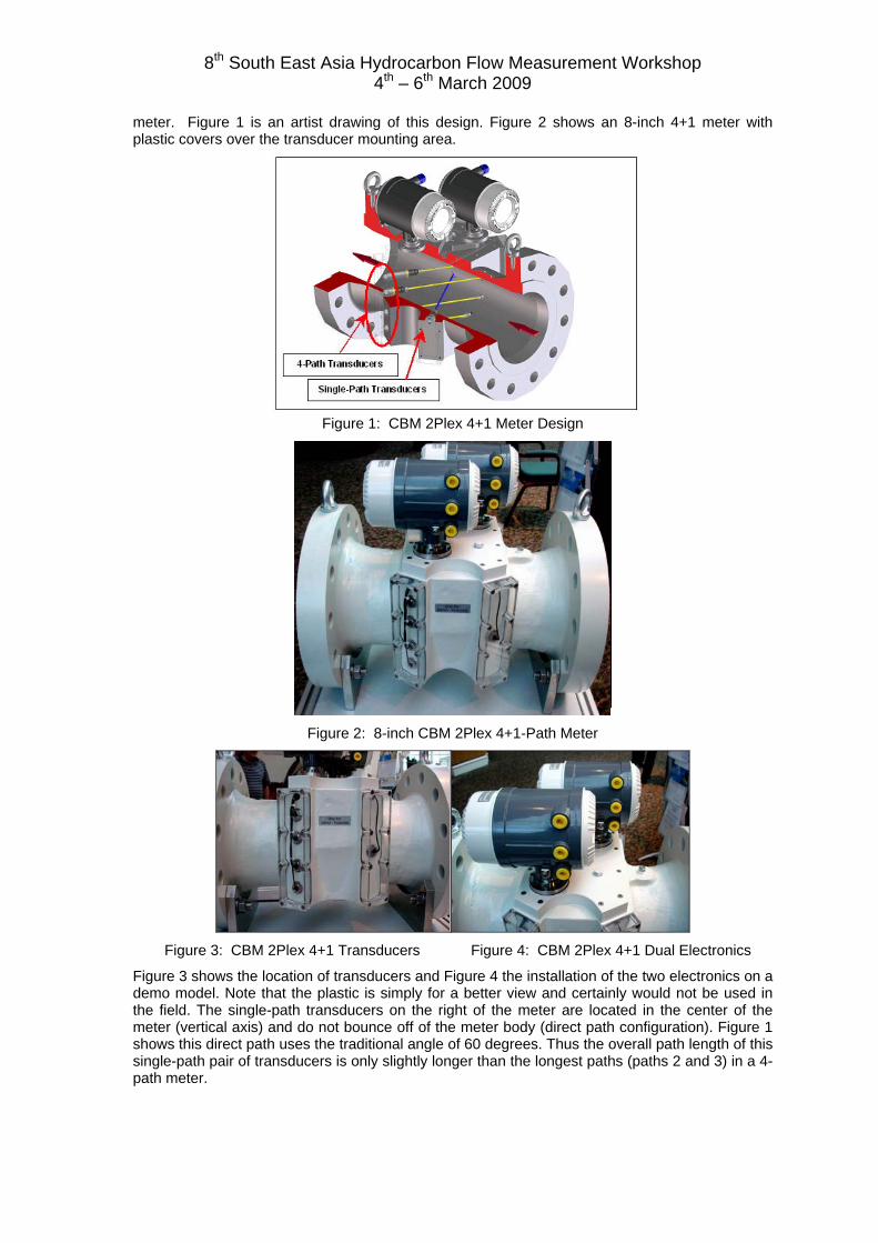
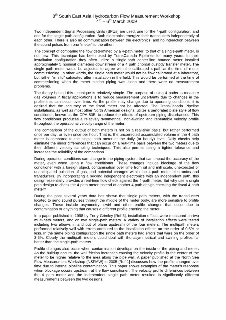
meter. Figure 1 is an artist drawing of this design. Figure 2 shows an 8-inch 4+1 meter withplastic covers over the transducer mounting area.

Figure 1: CBM 2Plex 4+1 Meter Design

Figure 2: 8-inch CBM 2Plex 4+1-Path Meter

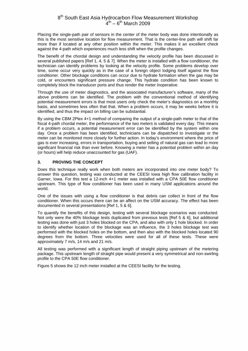
Figure 3: CBM 2Plex 4+1 Transducers Figure 4: CBM 2Plex 4+1 Dual Electronics

Figure 3 shows the location of transducers and Figure 4 the installation of the two electronics on ademo model. Note that the plastic is simply for a better view and certainly would not be used inthe field. The single-path transducers on the right of the meter are located in the center of themeter (vertical axis) and do not bounce off of the meter body (direct path configuration). Figure 1shows this direct path uses the traditional angle of 60 degrees. Thus the overall path length of thissingle-path pair of transducers is only slightly longer than the longest paths (paths 2 and 3) in a 4-path meter.


Two independent Signal Processing Units (SPUs) are used, one for the 4-path configuration, andone for the single-path configuration. Both electronics energize their transducers independently ofeach other. There is also no communication between the electronics, and no interaction betweenthe sound pulses from one “meter” to the other.

The concept of comparing the flow determined by a 4-path meter, to that of a single-path meter, isnot new. This technique has been used by TransCanada Pipelines for many years. In theirinstallation configuration they often utilize a single-path center-line bounce meter installedapproximately 5 nominal diameters downstream of a 4 path chordal custody transfer meter. Thesingle path meter would be adjusted to agree with the calibrated 4-path at the time of metercommissioning. In other words, the single path meter would not be flow calibrated at a laboratory,but rather “in situ” calibrated after installation in the field. This would be performed at the time ofcommissioning when the meter station piping was clean and there were no measurementproblems.

The theory behind this technique is relatively simple. The purpose of using 4 paths to measuregas volumes in fiscal applications is to reduce measurement uncertainty due to changes in theprofile that can occur over time. As the profile may change due to operating conditions, it isdesired that the accuracy of the fiscal meter not be affected. The TransCanada Pipelineinstallations, as well as most other North American designs, utilize a perforated plate style of flowconditioner, known as the CPA 50E, to reduce the effects of upstream piping disturbances. Thisflow conditioner produces a relatively symmetrical, non-swirling and repeatable velocity profilethroughout the operational velocity range of the meter.

The comparison of the output of both meters is not on a real-time basis, but rather performedonce per day, or even once per hour. That is, the uncorrected accumulated volume in the 4 pathmeter is compared to the single path meter at the daily (or hourly) level. Daily checks helpeliminate the minor differences that can occur on a real-time basis between the two meters due totheir different velocity sampling techniques. This also permits using a tighter tolerance andincreases the reliability of the comparison.

During operation conditions can change in the piping system that can impact the accuracy of themeter, even when using a flow conditioner. These changes include blockage of the flowconditioner with a foreign object, contamination over time from oil and mill scale, unexpected orunanticipated pulsation of gas, and potential changes within the 4-path meter electronics andtransducers. By incorporating a second independent electronics with an independent path, thisdesign essentially provides a real-time flow check against the 4-path meter. But why use a singlepath design to check the 4-path meter instead of another 4-path design checking the fiscal 4-pathmeter?

During the past several years data has shown that single path meters, with the transducerslocated to send sound pulses through the middle of the meter body, are more sensitive to profilechanges. These include asymmetry, swirl and other profile changes that occur due tocontamination or anything that causes a different profile entering the meter.

In a paper published in 1998 by Terry Grimley [Ref 3], installation effects were measured on twomulti-path meters, and on two single-path meters. A variety of installation effects were testedincluding two elbows in and out of plane upstream of the four meters. The multipath metersperformed relatively well with errors attributed to the installation effects on the order of 0.5% orless. In the same piping configuration the single path meters had errors that were on the order of2-5%. Clearly the multipath meters could deal with the asymmetrical and swirling profiles farbetter than the single-path meters.

Profile changes also occur when contamination develops on the inside of the piping and meter.As the buildup occurs, the wall friction increases causing the velocity profile in the center of themeter to be higher relative to the area along the pipe wall. A paper published at the North SeaFlow Measurement Workshop (NSFMW) in 2005 [Ref 1] discusses how the profile changed overtime due to internal pipeline contamination. This paper shows examples of the meter’s responsewhen blockage occurs upstream at the flow conditioner. The velocity profile differences betweenthe 4 path meter and the independent single path meter resulted in significantly differentmeasurements between the two designs.


Placing the single-path pair of sensors in the center of the meter body was done intentionally asthis is the most sensitive location for flow measurement. That is the center-line path will shift farmore than if located at any other position within the meter. This makes it an excellent checkagainst the 4-path which experiences much less shift when the profile changes.

The benefit of the chordal design and understanding the velocity profile has been discussed inseveral published papers [Ref 1, 4, 5 & 7]. When the meter is installed with a flow conditioner, thetechnician can identify problems by looking at the velocity profile. Some problems develop overtime, some occur very quickly as in the case of a foreign object lodging itself against the flowconditioner. Other blockage conditions can occur due to hydrate formation when the gas may becold, or encounters significant pressure change. This hydrate condition has been known tocompletely block the transducer ports and thus render the meter inoperative.

Through the use of meter diagnostics, and the associated manufacturer’s software, many of theabove problems can be identified. The problem with the conventional method of identifyingpotential measurement errors is that most users only check the meter’s diagnostics on a monthlybasis, and sometimes less often that that. When a problem occurs, it may be weeks before it isidentified, and thus the impact on billing can be substantial.

By using the CBM 2Plex 4+1 method of comparing the output of a single-path meter to that of thefiscal 4-path chordal meter, the performance of the two meters is validated every day. This meansif a problem occurs, a potential measurement error can be identified by the system within oneday. Once a problem has been identified, technicians can be dispatched to investigate or themeter can be monitored more closely for further action. In today’s environment where the price ofgas is ever increasing, errors in transportation, buying and selling of natural gas can lead to moresignificant financial risk than ever before. Knowing a meter has a potential problem within an day(or hours) will help reduce unaccounted for gas (UAF).

3. PROVING THE CONCEPT

Does this technique really work when both meters are incorporated into one meter body? Toanswer this question, testing was conducted at the CEESI Iowa high flow calibration facility inGarner, Iowa. For this test a 12-inch 4+1 meter was installed with a CPA 50E flow conditionerupstream. This type of flow conditioner has been used in many USM applications around theworld.

One of the issues with using a flow conditioner is that debris can collect in front of the flowconditioner. When this occurs there can be an affect on the USM accuracy. The effect has beendocumented in several presentations [Ref 1, 5 & 6].

To quantify the benefits of this design, testing with several blockage scenarios was conducted.Not only were the 40% blockage tests duplicated from previous tests [Ref 5 & 6], but additionaltesting was done with just 3 holes blocked on the CPA, and also with only 1 hole blocked. In orderto identify whether location of the blockage was an influence, the 3 holes blockage test wasperformed with the blocked holes on the bottom, and then also with the blocked holes located 90degrees from the bottom. Three velocities were used for all of these tests. These wereapproximately 7 m/s, 14 m/s and 21 m/s.

All testing was performed with a significant length of straight piping upstream of the meteringpackage. This upstream length of straight pipe would present a very symmetrical and non-swirlingprofile to the CPA 50E flow conditioner.

Figure 5 shows the 12 inch meter installed at the CEESI facility for the testing.


Figure 5: 12-inch 4+1 CBM Meter CEESI

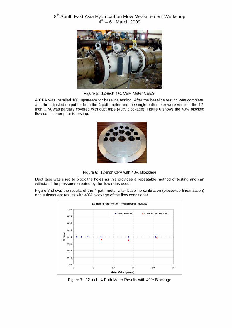
A CPA was installed 10D upstream for baseline testing. After the baseline testing was complete,and the adjusted output for both the 4 path meter and the single path meter were verified, the 12-inch CPA was partially covered with duct tape (40% blockage). Figure 6 shows the 40% blockedflow conditioner prior to testing.

Figure 6: 12-inch CPA with 40% Blockage

Duct tape was used to block the holes as this provides a repeatable method of testing and canwithstand the pressures created by the flow rates used.

Figure 7 shows the results of the 4-path meter after baseline calibration (piecewise linearization)and subsequent results with 40% blockage of the flow conditioner.

12-inch, 4-Path Meter - 40% Blocked Results

-1.00

-0.75

-0.50

-0.25

0.00

0.25

0.50

0.75

1.00

0 5 10 15 20 25

Meter Velocity (m/s)

% E

rror

Un-Blocked CPA 40 Percent Blocked CPA

Figure 7: 12-inch, 4-Path Meter Results with 40% Blockage


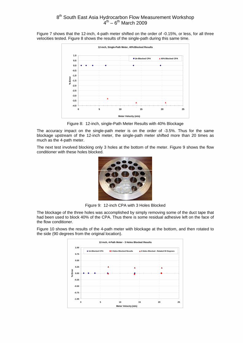
Figure 7 shows that the 12-inch, 4-path meter shifted on the order of -0.15%, or less, for all threevelocities tested. Figure 8 shows the results of the single-path during this same time.

12-inch, Single-Path Meter, 40% Blocked Results

-4.0

-3.5

-3.0

-2.5

-2.0

-1.5

-1.0

-0.5

0.0

0.5

1.0

0 5 10 15 20 25


% E

rror

Un-Blocked CPA 40% Blocked CPA

Figure 8: 12-inch, single-Path Meter Results with 40% Blockage

The accuracy impact on the single-path meter is on the order of -3.5%. Thus for the sameblockage upstream of the 12-inch meter, the single-path meter shifted more than 20 times asmuch as the 4-path meter.

The next test involved blocking only 3 holes at the bottom of the meter. Figure 9 shows the flowconditioner with these holes blocked.

Figure 9: 12-inch CPA with 3 Holes Blocked

The blockage of the three holes was accomplished by simply removing some of the duct tape thathad been used to block 40% of the CPA. Thus there is some residual adhesive left on the face ofthe flow conditioner.

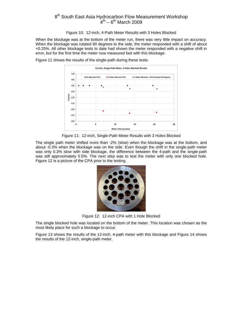
Figure 10 shows the results of the 4-path meter with blockage at the bottom, and then rotated tothe side (90 degrees from the original location).

12-inch, 4-Path Meter - 3 Holes Blocked Results

-1.00

-0.75

-0.50

-0.25

0.00

0.25

0.50

0.75

1.00

0 5 10 15 20 25


% E

rror

Un-Blocked CPA 3 Holes Blocked Results 3 Holes Blocked - Rotated 90 Degrees


Figure 10: 12-inch, 4-Path Meter Results with 3 Holes Blocked

When the blockage was at the bottom of the meter run, there was very little impact on accuracy.When the blockage was rotated 90 degrees to the side, the meter responded with a shift of about+0.25%. All other blockage tests to date had shown the meter responded with a negative shift inerror, but for the first time the meter now measured fast with this blockage.

Figure 11 shows the results of the single-path during these tests.

12-inch, Single-Path Meter, 3 Holes Blocked Results

-3.0

-2.5

-2.0

-1.5

-1.0

-0.5

0.0

0.5

1.0

0 5 10 15 20 25


% E

rror

Un-Blocked CPA 3 Holes Blocked CPA 3 Holes Blocked - CPA Rotated 90 Degrees

`

Figure 11: 12-inch, Single-Path Meter Results with 3 Holes Blocked

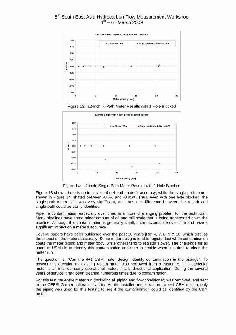
The single path meter shifted more than -2% (slow) when the blockage was at the bottom, andabout -0.3% when the blockage was on the side. Even though the shift in the single-path meterwas only 0.3% slow with side blockage, the difference between the 4-path and the single-pathwas still approximately 0.5%. The next step was to test the meter with only one blocked hole.Figure 12 is a picture of the CPA prior to the testing.

Figure 12: 12-inch CPA with 1 Hole Blocked

The single blocked hole was located on the bottom of the meter. This location was chosen as themost likely place for such a blockage to occur.

Figure 13 shows the results of the 12-inch, 4-path meter with this blockage and Figure 14 showsthe results of the 12-inch, single-path meter.


12-inch, 4-Path Meter - 1 Hole Blocked Results

-1.00

-0.75

-0.50

-0.25

0.00

0.25

0.50

0.75

1.00

0 5 10 15 20 25Meter Velocity (m/s)

% E

rror

Un-Blocked CPA Single Hole Blocked - Botton CPA

Figure 13: 12-inch, 4-Path Meter Results with 1 Hole Blocked

12-inch, Single-Path Meter, 1 Hole Blocked Results

-1.00

-0.75

-0.50

-0.25

0.00

0.25

0.50

0.75

1.00

0 5 10 15 20 25


% E

rror

Un-Blocked CPA Single Hole Blocked - Bottom CPA

Figure 14: 12-inch, Single-Path Meter Results with 1 Hole Blocked

Figure 13 shows there is no impact on the 4-path meter’s accuracy, while the single-path meter,shown in Figure 14, shifted between -0.6% and -0.85%. Thus, even with one hole blocked, thesingle-path meter shift was very significant, and thus the difference between the 4-path andsingle-path could be easily identified.

Pipeline contamination, especially over time, is a more challenging problem for the technician.Many pipelines have some minor amount of oil and mill scale that is being transported down thepipeline. Although this contamination is generally small, it can accumulate over time and have asignificant impact on a meter’s accuracy.

Several papers have been published over the past 10 years [Ref 4, 7, 8, 9 & 10] which discussthe impact on the meter’s accuracy. Some meter designs tend to register fast when contaminationcoats the meter piping and meter body, while others tend to register slower. The challenge for allusers of USMs is to identify this contamination and then to decide when it is time to clean themeter run.

The question is: “Can the 4+1 CBM meter design identify contamination in the piping?”. Toanswer this question an existing 4-path meter was borrowed from a customer. This particularmeter is an inter-company operational meter, in a bi-directional application. During the severalyears of service it had been cleaned numerous times due to contamination.

For this test the entire meter run (including all piping and flow conditioner) was removed, and sentto the CEESI Garner calibration facility. As the installed meter was not a 4+1 CBM design, onlythe piping was used for this testing to see if the contamination could be identified by the CBMmeter.


As this meter was installed in the late 1990’s, it used a 19-tube bundle. Figures 15 and 16 showthe 19-tube flow conditioner during disassembly at the CEESI facility.

Figure 15: 19-Tube Bundle Figure 16: Close-up of 19-Tube Bundle

Unfortunately the meter run had been cleaned recently and the upstream piping was not as dirtyas was expected. Figure 17 shows the “as-found” condition of the piping between the flowconditioner (19-tube bundle) and the meter.

Figure 17: 12-inch Dirty Piping

As Figure 17 shows, there was not a lot of contamination remaining due to the recent cleaning ofthe meter piping. This was a bit of a disappointment for the customer as they expected the pipingto be a bit dirtier.

Figure 18 is a close up of one of the meter pipes prior to any cleaning.

Figure 18: 12-inch Dirty Piping Close Up

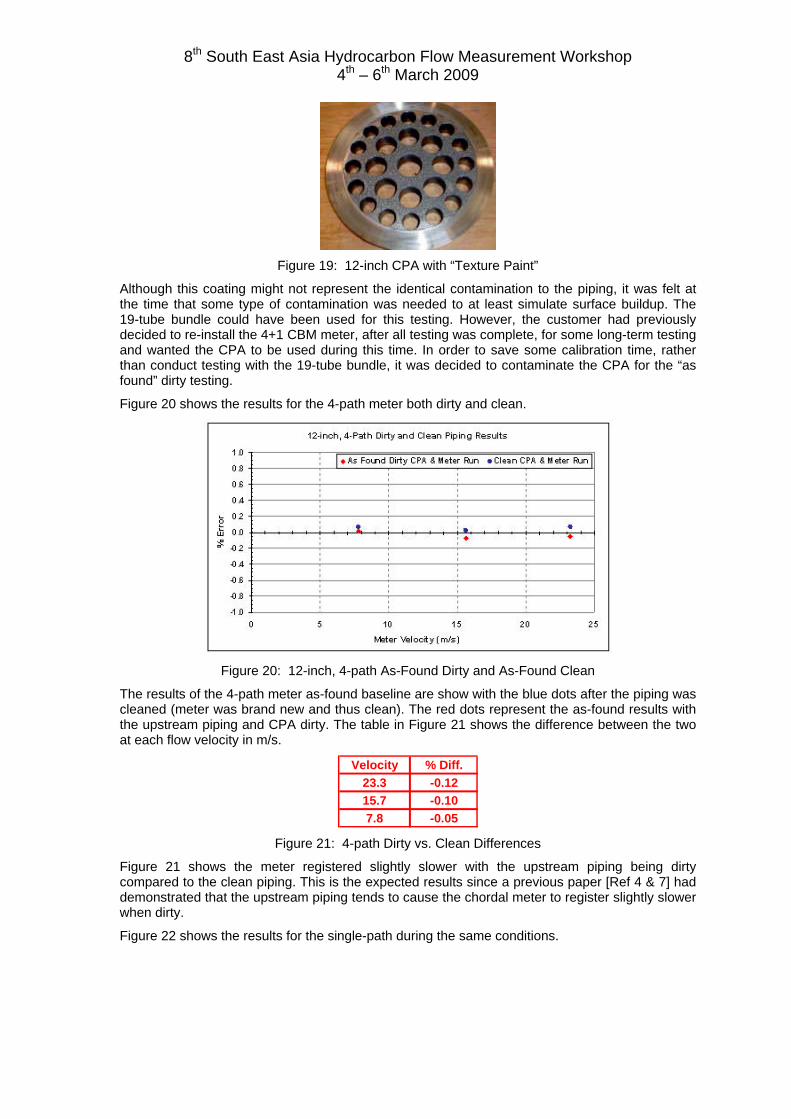
Today most designers do not use this type of flow conditioner but instead select a perforated platelike the CPA 50E. The customer chose to re-install the meter after testing and replace the 19-tubebundle with the CPA unit. For this reason all testing was conducted with a CPA flow conditioner.To simulate what the flow conditioner may have looked like if it been subjected to normal pipelinecontamination, “texture” paint was applied to the CPA flow conditioner. Figure 19 shows the flowconditioner just prior to being installed for the testing.


Figure 19: 12-inch CPA with “Texture Paint”

Although this coating might not represent the identical contamination to the piping, it was felt atthe time that some type of contamination was needed to at least simulate surface buildup. The19-tube bundle could have been used for this testing. However, the customer had previouslydecided to re-install the 4+1 CBM meter, after all testing was complete, for some long-term testingand wanted the CPA to be used during this time. In order to save some calibration time, ratherthan conduct testing with the 19-tube bundle, it was decided to contaminate the CPA for the “asfound” dirty testing.

Figure 20 shows the results for the 4-path meter both dirty and clean.

Figure 20: 12-inch, 4-path As-Found Dirty and As-Found Clean

The results of the 4-path meter as-found baseline are show with the blue dots after the piping wascleaned (meter was brand new and thus clean). The red dots represent the as-found results withthe upstream piping and CPA dirty. The table in Figure 21 shows the difference between the twoat each flow velocity in m/s.

Velocity % Diff.23.3 -0.1215.7 -0.107.8 -0.05

Figure 21: 4-path Dirty vs. Clean Differences

Figure 21 shows the meter registered slightly slower with the upstream piping being dirtycompared to the clean piping. This is the expected results since a previous paper [Ref 4 & 7] haddemonstrated that the upstream piping tends to cause the chordal meter to register slightly slowerwhen dirty.

Figure 22 shows the results for the single-path during the same conditions.


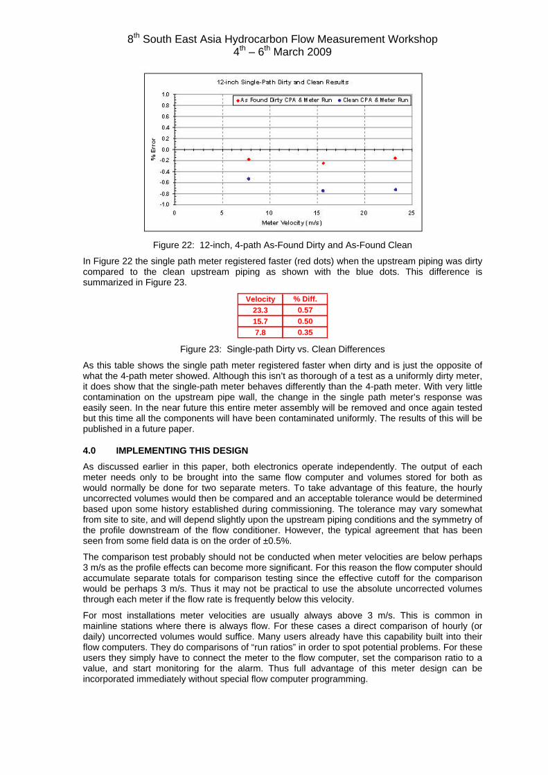
Figure 22: 12-inch, 4-path As-Found Dirty and As-Found Clean

In Figure 22 the single path meter registered faster (red dots) when the upstream piping was dirtycompared to the clean upstream piping as shown with the blue dots. This difference issummarized in Figure 23.

Velocity % Diff.23.3 0.5715.7 0.507.8 0.35

Figure 23: Single-path Dirty vs. Clean Differences

As this table shows the single path meter registered faster when dirty and is just the opposite ofwhat the 4-path meter showed. Although this isn’t as thorough of a test as a uniformly dirty meter,it does show that the single-path meter behaves differently than the 4-path meter. With very littlecontamination on the upstream pipe wall, the change in the single path meter’s response waseasily seen. In the near future this entire meter assembly will be removed and once again testedbut this time all the components will have been contaminated uniformly. The results of this will bepublished in a future paper.

4.0 IMPLEMENTING THIS DESIGN

As discussed earlier in this paper, both electronics operate independently. The output of eachmeter needs only to be brought into the same flow computer and volumes stored for both aswould normally be done for two separate meters. To take advantage of this feature, the hourlyuncorrected volumes would then be compared and an acceptable tolerance would be determinedbased upon some history established during commissioning. The tolerance may vary somewhatfrom site to site, and will depend slightly upon the upstream piping conditions and the symmetry ofthe profile downstream of the flow conditioner. However, the typical agreement that has beenseen from some field data is on the order of ±0.5%.

The comparison test probably should not be conducted when meter velocities are below perhaps3 m/s as the profile effects can become more significant. For this reason the flow computer shouldaccumulate separate totals for comparison testing since the effective cutoff for the comparisonwould be perhaps 3 m/s. Thus it may not be practical to use the absolute uncorrected volumesthrough each meter if the flow rate is frequently below this velocity.

For most installations meter velocities are usually always above 3 m/s. This is common inmainline stations where there is always flow. For these cases a direct comparison of hourly (ordaily) uncorrected volumes would suffice. Many users already have this capability built into theirflow computers. They do comparisons of “run ratios” in order to spot potential problems. For theseusers they simply have to connect the meter to the flow computer, set the comparison ratio to avalue, and start monitoring for the alarm. Thus full advantage of this meter design can beincorporated immediately without special flow computer programming.


Some users have algorithms in their data acquisition system that permit comparing volumes fromone meter run to another when they are in parallel operation. This has been very helpful inidentifying problems with orifice and turbine measurement. Essentially the system can beprogrammed to compare the hourly or daily volume between parallel runs and then alarm whenthe volume is outside of a specified tolerance. As other technologies don’t have the diagnostics ofan ultrasonic meter, this was perhaps the best solution to monitor potential problems.

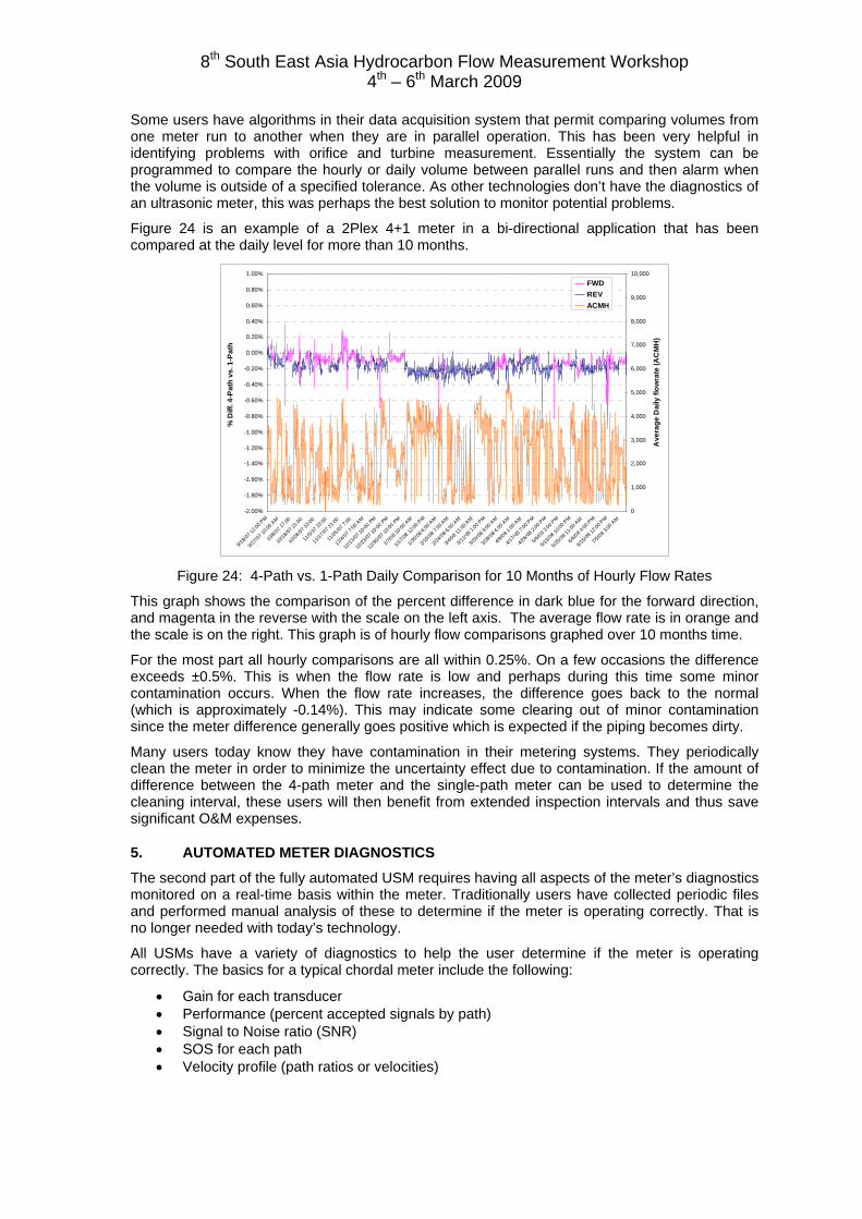
Figure 24 is an example of a 2Plex 4+1 meter in a bi-directional application that has beencompared at the daily level for more than 10 months.

-2.00%

-1.80%

-1.60%

-1.40%

-1.20%

-1.00%

-0.80%

-0.60%

-0.40%

-0.20%

0.00%

0.20%

0.40%

0.60%

0.80%

1.00%

9/18/0

7 12:0

0 PM

9/27/0

7 10:0

0 AM

10/8/

07 17

:00

10/18

/07 21

:00

10/28

/07 10

:00

11/5/

07 22

:00

11/17

/07 21

:00

11/25

/07 7:

00

12/4/

07 7:

00 A

M

12/13

/07 10

:00 PM

12/23

/07 10

:00 PM

12/30

/07 10

:00 PM

1/7/08 1

0:00 A

M

1/17/0

8 12:0

0 PM

1/30/0

8 6:00

AM

2/15/0

8 7:00

AM

2/24/0

8 6:00

AM

3/4/08 1

1:00 A

M

3/11/0

8 1:00

PM

3/20/0

8 9:00

AM

3/28/0

8 6:00

AM

4/9/08 1

:00 A

M

4/17/0

8 7:00

PM

4/26/0

8 2:00

PM

5/6/08 3

:00 P

M

5/13/0

8 10:0

0 PM

5/25/0

8 11:0

0 AM

6/6/08 4

:00 P

M

6/15/0

8 12:0

0 PM

7/5/08 3

:00 A

M

% D

iff. 4

-Pat

h vs

. 1-P

ath

0

1,000

2,000

3,000

4,000

5,000

6,000

7,000

8,000

9,000

10,000

Ave

rage

Dai

ly fl

owra

te (A

CM

H)

FWDREVACMH

Figure 24: 4-Path vs. 1-Path Daily Comparison for 10 Months of Hourly Flow Rates

This graph shows the comparison of the percent difference in dark blue for the forward direction,and magenta in the reverse with the scale on the left axis. The average flow rate is in orange andthe scale is on the right. This graph is of hourly flow comparisons graphed over 10 months time.

For the most part all hourly comparisons are all within 0.25%. On a few occasions the differenceexceeds ±0.5%. This is when the flow rate is low and perhaps during this time some minorcontamination occurs. When the flow rate increases, the difference goes back to the normal(which is approximately -0.14%). This may indicate some clearing out of minor contaminationsince the meter difference generally goes positive which is expected if the piping becomes dirty.

Many users today know they have contamination in their metering systems. They periodicallyclean the meter in order to minimize the uncertainty effect due to contamination. If the amount ofdifference between the 4-path meter and the single-path meter can be used to determine thecleaning interval, these users will then benefit from extended inspection intervals and thus savesignificant O&M expenses.

5. AUTOMATED METER DIAGNOSTICS

The second part of the fully automated USM requires having all aspects of the meter’s diagnosticsmonitored on a real-time basis within the meter. Traditionally users have collected periodic filesand performed manual analysis of these to determine if the meter is operating correctly. That isno longer needed with today’s technology.

All USMs have a variety of diagnostics to help the user determine if the meter is operatingcorrectly. The basics for a typical chordal meter include the following:

• Gain for each transducer• Performance (percent accepted signals by path)• Signal to Noise ratio (SNR)• SOS for each path• Velocity profile (path ratios or velocities)


Today these 5 are enhanced by additional diagnostics for the user to better understand if themeter is operating correctly. These include the following:

• Profile Factor• Symmetry• Turbulence

Profile factor and Symmetry are methods of analyzing the velocity profile (or path ratios). Theyare values which reflect the shape and amount of distortion in the basic velocity profile. Theyhave been used for years to help understand the velocity profile which is often considered bymany to be the most difficult diagnostic to understand [Ref 2 & 12]. These two are defined asfollows:

• Profile Factor = (Path 2 + Path 3) / (Path 1 + Path 4)• Symmetry = (Path 1 + Path 2) / (Path 3 + Path 4)

Many consider a meter’s velocity profile the most difficult to understand because it can vary dueto installation and type of upstream piping components, and to some degree, flow rate. Generallyspeaking these two diagnostics (Profile Factor and Symmetry) are very stable above a velocity ofapproximately 2-3 m/s.

However, this is only true if the piping design incorporates a flow conditioner like the onediscussed earlier in this paper. Without a flow conditioner, the velocity profile will have a widerange of both Profile Factor and Symmetry, and thus very difficult, if not impractical, to monitorand alarm on these value.

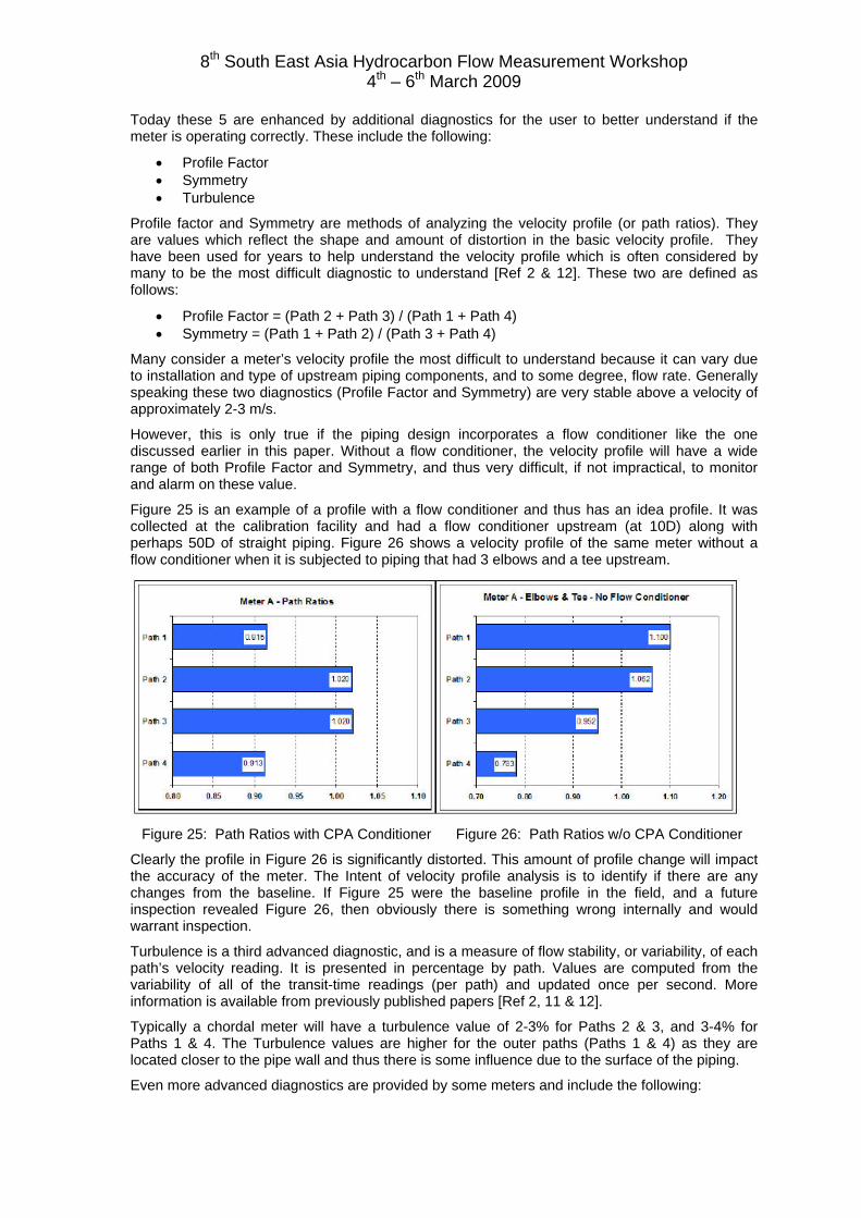
Figure 25 is an example of a profile with a flow conditioner and thus has an idea profile. It wascollected at the calibration facility and had a flow conditioner upstream (at 10D) along withperhaps 50D of straight piping. Figure 26 shows a velocity profile of the same meter without aflow conditioner when it is subjected to piping that had 3 elbows and a tee upstream.

Figure 25: Path Ratios with CPA Conditioner Figure 26: Path Ratios w/o CPA Conditioner

Clearly the profile in Figure 26 is significantly distorted. This amount of profile change will impactthe accuracy of the meter. The Intent of velocity profile analysis is to identify if there are anychanges from the baseline. If Figure 25 were the baseline profile in the field, and a futureinspection revealed Figure 26, then obviously there is something wrong internally and wouldwarrant inspection.

Turbulence is a third advanced diagnostic, and is a measure of flow stability, or variability, of eachpath’s velocity reading. It is presented in percentage by path. Values are computed from thevariability of all of the transit-time readings (per path) and updated once per second. Moreinformation is available from previously published papers [Ref 2, 11 & 12].

Typically a chordal meter will have a turbulence value of 2-3% for Paths 2 & 3, and 3-4% forPaths 1 & 4. The Turbulence values are higher for the outer paths (Paths 1 & 4) as they arelocated closer to the pipe wall and thus there is some influence due to the surface of the piping.

Even more advanced diagnostics are provided by some meters and include the following:


• High meter velocity (exceeding programmed limit)• Power supply voltage too low (below a programmed value)• Logbook(s) warning when full of un-acknowledged entries

These previously identified advanced diagnostics, and more, can now be fully automated in themeter by having site-specific programmed values for each diagnostic parameter.

There are many benefits to having these programmed in the meter rather than in the User’ssoftware or in a flow computer. Knowing within minutes that a problem may exist significantlyreduces measurement uncertainty. Some of the many benefits include:

• The meter monitors all parameters/diagnostics on a real-time basis. When a diagnostic isapproaching a limit, the meter then presents an alarm that can be remotely monitored.

• If diagnostic limits established in meter’s software (User interface), the only time the userwill know there is a problem is when they are connected to the meter. As a result themeter can operate for weeks with a problem before a technician might identify it.

• Each location, and meter size, will have different limits due to the station design, metersize, pressure, flow rates, etc. By having these programmed in the meter, they can betailored to the site-specific conditions and thus present an alarm more quickly andaccurately.

• One additional benefit of having the meter do this, rather than the flow computer or RTU,is that no additional programming is required. Simply monitor a digital output (DO) and theRTU can then report if there is a problem with a diagnostic. This saves the user time andmoney and makes implementing this feature very easy.

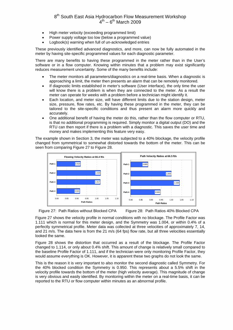
The example shown in Section 3, the meter was subjected to a 40% blockage, the velocity profilechanged from symmetrical to somewhat distorted towards the bottom of the meter. This can beseen from comparing Figure 27 to Figure 28.

Flowing Velocity Ratios at 66.4 ft/s

0.919

1.020

1.017

0.915

0.80 0.85 0.90 0.95 1.00 1.05 1.10

Path 1

Path 2

Path 3

Path 4

Path Ratios

Path Velocity Ratios at 66.5 ft/s

0.885

1.000

1.039

0.945

0.80 0.85 0.90 0.95 1.00 1.05 1.10

Path 1

Path 2

Path 3

Path 4

Path Ratios

Figure 27: Path Ratios without Blocked CPA Figure 28: Path Ratios 40% Blocked CPA

Figure 27 shows the velocity profile in normal conditions with no blockage. The Profile Factor was1.111 which is normal for this meter design, and the Symmetry was 1.004, or within 0.4% of aperfectly symmetrical profile. Meter data was collected at three velocities of approximately 7, 14,and 21 m/s. The data here is from the 21 m/s (64 fps) flow rate, but all three velocities essentiallylooked the same.

Figure 28 shows the distortion that occurred as a result of the blockage. The Profile Factorchanged to 1.114, or only about 0.4% shift. This amount of change is relatively small compared tothe baseline Profile Factor of 1.111, and if the technician were only monitoring Profile Factor, theywould assume everything is OK. However, it is apparent these two graphs do not look the same.

This is the reason it is very important to also monitor the second diagnostic called Symmetry. Forthe 40% blocked condition the Symmetry is 0.950. This represents about a 5.5% shift in thevelocity profile towards the bottom of the meter (high velocity average). This magnitude of changeis very obvious and easily identified. By monitoring within the meter on a real-time basis, it can bereported to the RTU or flow computer within minutes as an abnormal profile.


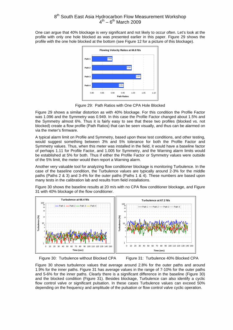
One can argue that 40% blockage is very significant and not likely to occur often. Let’s look at theprofile with only one hole blocked as was presented earlier in this paper. Figure 29 shows theprofile with the one hole blocked at the bottom (see Figure 12 for a picture of this blockage).

Flowing Velocity Ratios at 66.8 ft/s

0.898

0.992

1.037

0.954

0.80 0.85 0.90 0.95 1.00 1.05 1.10

Path 1

Path 2

Path 3

Path 4

Path Ratios

Figure 29: Path Ratios with One CPA Hole Blocked

Figure 29 shows a similar distortion as with 40% blockage. For this condition the Profile Factorwas 1.096 and the Symmetry was 0.949. In this case the Profile Factor changed about 1.5% andthe Symmetry almost 6%. Thus it is fairly easy to see that these two profiles (blocked vs. notblocked) create a flow profile (Path Ratios) that can be seen visually, and thus can be alarmed onvia the meter’s firmware.

A typical alarm limit on Profile and Symmetry, based upon these test conditions, and other testing,would suggest something between 3% and 5% tolerance for both the Profile Factor andSymmetry values. Thus, when this meter was installed in the field, it would have a baseline factorof perhaps 1.11 for Profile Factor, and 1.005 for Symmetry, and the Warning alarm limits wouldbe established at 5% for both. Thus if either the Profile Factor or Symmetry values were outsideof the 5% limit, the meter would then report a Warning alarm.

Another very valuable tool for analyzing flow conditioner blockage is monitoring Turbulence. In thecase of the baseline condition, the Turbulence values are typically around 2-3% for the middlepaths (Paths 2 & 3) and 3-4% for the outer paths (Paths 1 & 4). These numbers are based uponmany tests in the calibration lab and results from field installations.

Figure 30 shows the baseline results at 20 m/s with no CPA flow conditioner blockage, and Figure31 with 40% blockage of the flow conditioner.

Turbulence at 66.4 ft/s

2

4

68

20

40

6080

1

10

100

0 10 20 30 40 50 60 70 80 90 100 110 120 130 140 150

Time (sec)

Turb

ulen

ce (%

)

Path 1 Path 2 Path 3 Path 4


2

4

68

20

40

6080

1

10

100

0 10 20 30 40 50 60 70 80 90 100 110 120 130 140 150

Time (sec)

Turb

ulen

ce (%

)


Figure 30: Turbulence without Blocked CPA Figure 31: Turbulence 40% Blocked CPA

Figure 30 shows turbulence values that average around 2.8% for the outer paths and around1.9% for the inner paths. Figure 31 has average values in the range of 7-10% for the outer pathsand 5-6% for the inner paths. Clearly there is a significant difference in the baseline (Figure 30)and the blocked condition (Figure 31). Besides blockage, Turbulence can also identify a cyclicflow control valve or significant pulsation. In these cases Turbulence values can exceed 50%depending on the frequency and amplitude of the pulsation or flow control valve cyclic operation.


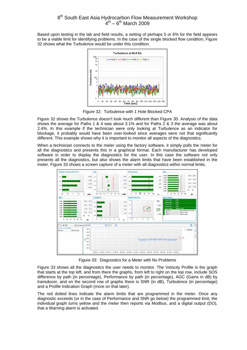
Based upon testing in the lab and field results, a setting of perhaps 5 or 6% for the field appearsto be a viable limit for identifying problems. In the case of the single blocked flow condition, Figure32 shows what the Turbulence would be under this condition.


2

4

68

20

40

6080

1

10

100

0 10 20 30 40 50 60 70 80 90 100 110 120 130 140 150Time (sec)

Turb

ulen

ce (%

)


Figure 32: Turbulence with 1 Hole Blocked CPA

Figure 32 shows the Turbulence doesn’t look much different than Figure 30. Analysis of the datashows the average for Paths 1 & 4 was about 3.1% and for Paths 2 & 3 the average was about2.4%. In this example if the technician were only looking at Turbulence as an indicator forblockage, it probably would have been over-looked since averages were not that significantlydifferent. This example shows why it is important to monitor all aspects of the diagnostics.

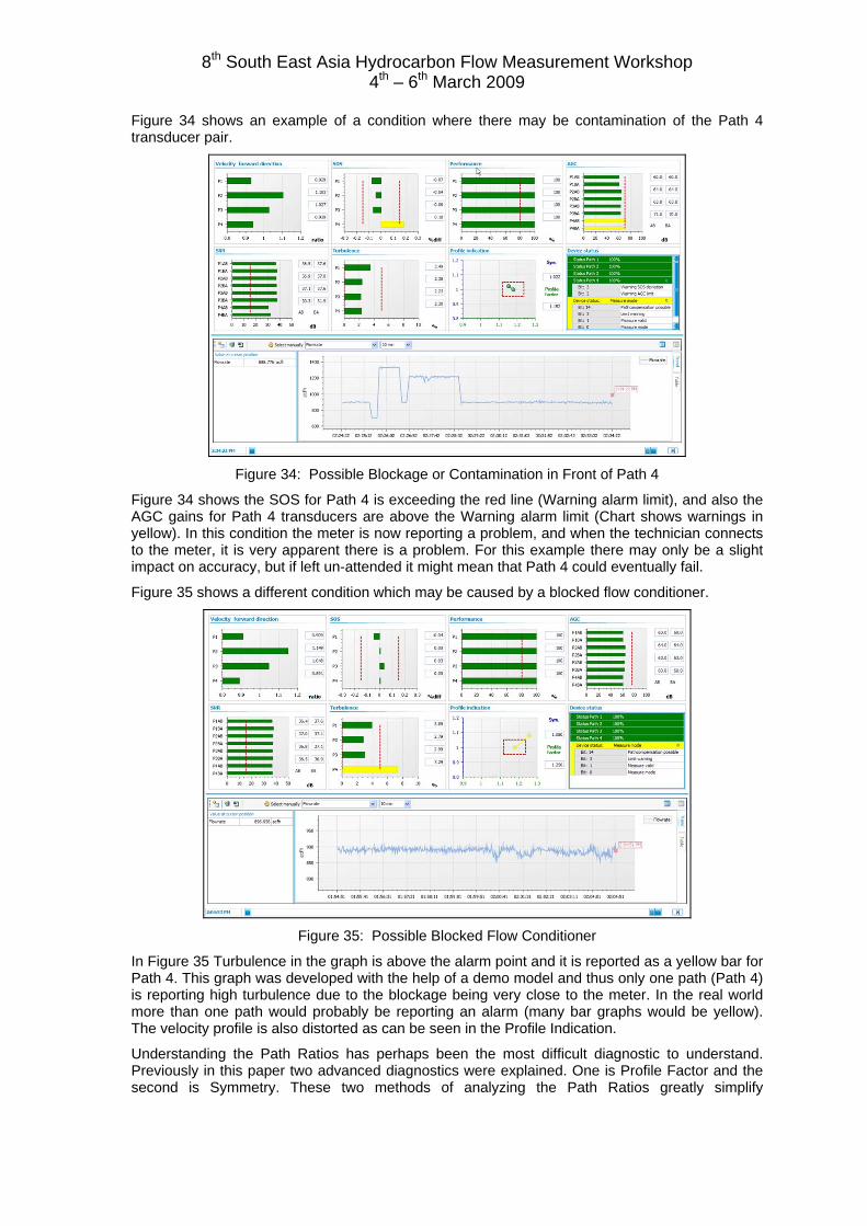
When a technician connects to the meter using the factory software, it simply polls the meter forall the diagnostics and presents this in a graphical format. Each manufacturer has developedsoftware in order to display the diagnostics for the user. In this case the software not onlypresents all the diagnostics, but also shows the alarm limits that have been established in themeter. Figure 33 shows a screen capture of a meter with all diagnostics within normal limits.

Figure 33: Diagnostics for a Meter with No Problems

Figure 33 shows all the diagnostics the user needs to monitor. The Velocity Profile is the graphthat starts at the top left, and from there the graphs, from left to right on the top row, include SOSdifference by path (in percentage), Performance by path (in percentage), AGC (Gains in dB) bytransducer, and on the second row of graphs there is SNR (in dB), Turbulence (in percentage)and a Profile Indication Graph (more on that later).

The red dotted lines indicate the alarm limits that are programmed in the meter. Once anydiagnostic exceeds (or in the case of Performance and SNR go below) the programmed limit, theindividual graph turns yellow and the meter then reports via Modbus, and a digital output (DO),that a Warning alarm is activated.


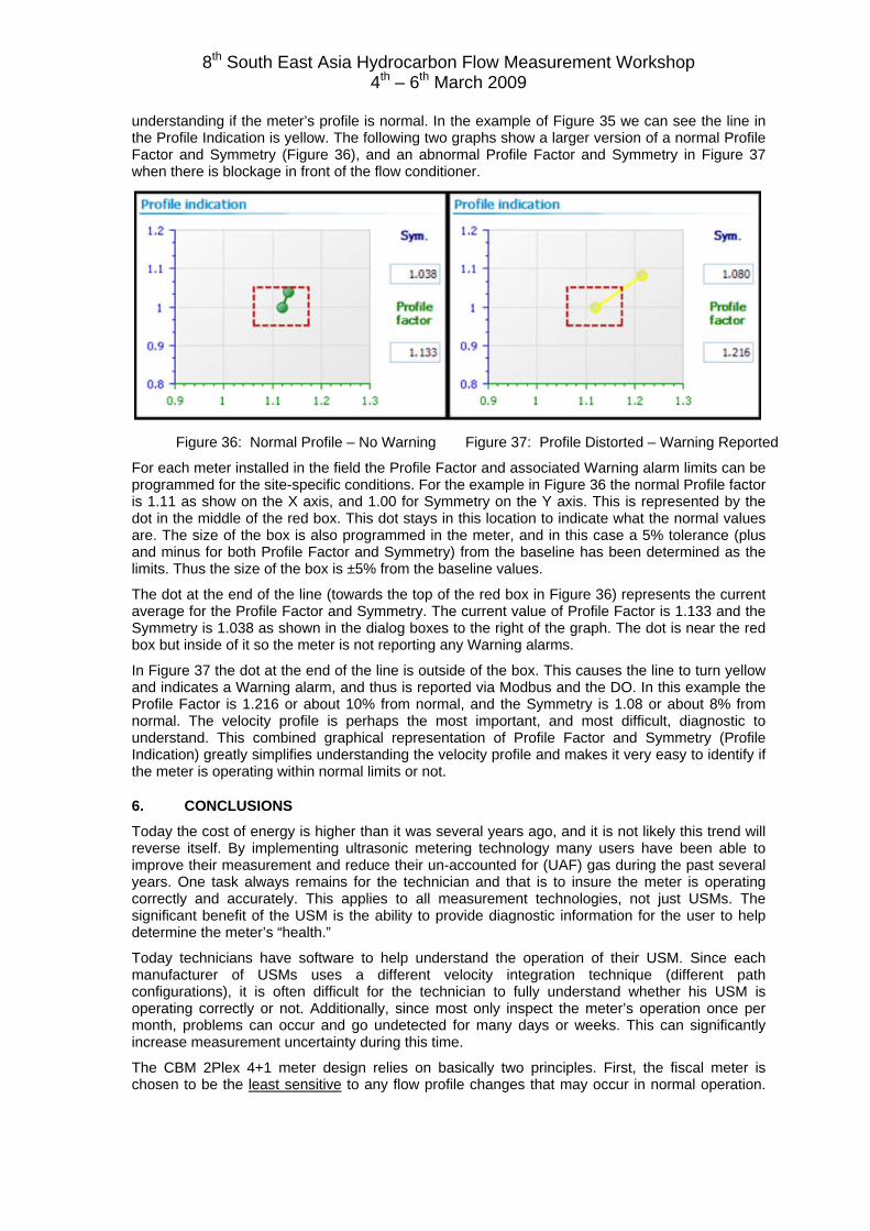
Figure 34 shows an example of a condition where there may be contamination of the Path 4transducer pair.

Figure 34: Possible Blockage or Contamination in Front of Path 4

Figure 34 shows the SOS for Path 4 is exceeding the red line (Warning alarm limit), and also theAGC gains for Path 4 transducers are above the Warning alarm limit (Chart shows warnings inyellow). In this condition the meter is now reporting a problem, and when the technician connectsto the meter, it is very apparent there is a problem. For this example there may only be a slightimpact on accuracy, but if left un-attended it might mean that Path 4 could eventually fail.

Figure 35 shows a different condition which may be caused by a blocked flow conditioner.

Figure 35: Possible Blocked Flow Conditioner

In Figure 35 Turbulence in the graph is above the alarm point and it is reported as a yellow bar forPath 4. This graph was developed with the help of a demo model and thus only one path (Path 4)is reporting high turbulence due to the blockage being very close to the meter. In the real worldmore than one path would probably be reporting an alarm (many bar graphs would be yellow).The velocity profile is also distorted as can be seen in the Profile Indication.

Understanding the Path Ratios has perhaps been the most difficult diagnostic to understand.Previously in this paper two advanced diagnostics were explained. One is Profile Factor and thesecond is Symmetry. These two methods of analyzing the Path Ratios greatly simplify


understanding if the meter’s profile is normal. In the example of Figure 35 we can see the line inthe Profile Indication is yellow. The following two graphs show a larger version of a normal ProfileFactor and Symmetry (Figure 36), and an abnormal Profile Factor and Symmetry in Figure 37when there is blockage in front of the flow conditioner.

Figure 36: Normal Profile – No Warning Figure 37: Profile Distorted – Warning Reported

For each meter installed in the field the Profile Factor and associated Warning alarm limits can beprogrammed for the site-specific conditions. For the example in Figure 36 the normal Profile factoris 1.11 as show on the X axis, and 1.00 for Symmetry on the Y axis. This is represented by thedot in the middle of the red box. This dot stays in this location to indicate what the normal valuesare. The size of the box is also programmed in the meter, and in this case a 5% tolerance (plusand minus for both Profile Factor and Symmetry) from the baseline has been determined as thelimits. Thus the size of the box is ±5% from the baseline values.

The dot at the end of the line (towards the top of the red box in Figure 36) represents the currentaverage for the Profile Factor and Symmetry. The current value of Profile Factor is 1.133 and theSymmetry is 1.038 as shown in the dialog boxes to the right of the graph. The dot is near the redbox but inside of it so the meter is not reporting any Warning alarms.

In Figure 37 the dot at the end of the line is outside of the box. This causes the line to turn yellowand indicates a Warning alarm, and thus is reported via Modbus and the DO. In this example theProfile Factor is 1.216 or about 10% from normal, and the Symmetry is 1.08 or about 8% fromnormal. The velocity profile is perhaps the most important, and most difficult, diagnostic tounderstand. This combined graphical representation of Profile Factor and Symmetry (ProfileIndication) greatly simplifies understanding the velocity profile and makes it very easy to identify ifthe meter is operating within normal limits or not.

6. CONCLUSIONS

Today the cost of energy is higher than it was several years ago, and it is not likely this trend willreverse itself. By implementing ultrasonic metering technology many users have been able toimprove their measurement and reduce their un-accounted for (UAF) gas during the past severalyears. One task always remains for the technician and that is to insure the meter is operatingcorrectly and accurately. This applies to all measurement technologies, not just USMs. Thesignificant benefit of the USM is the ability to provide diagnostic information for the user to helpdetermine the meter’s “health.”

Today technicians have software to help understand the operation of their USM. Since eachmanufacturer of USMs uses a different velocity integration technique (different pathconfigurations), it is often difficult for the technician to fully understand whether his USM isoperating correctly or not. Additionally, since most only inspect the meter’s operation once permonth, problems can occur and go undetected for many days or weeks. This can significantlyincrease measurement uncertainty during this time.

The CBM 2Plex 4+1 meter design relies on basically two principles. First, the fiscal meter ischosen to be the least sensitive to any flow profile changes that may occur in normal operation.


And second, the “check” meter design is chosen to be one that is the most sensitive to any flowprofile changes. Ideally any affect from a profile change would not only have a significantlydifferent impact on accuracy for each path layout, but the affect would be in opposite directions,making the difference much easier to detect.

The benefit of the CBM 2Plex 4+1 meter design is that the flow computer is used to check thehealth of the fiscal 4-path chordal meter by simply comparing it to the single-path meter. If thevelocity profile remains relatively constant, both meters will agree. Should some process conditionupset the normal profile, the single-path meter will respond significantly different than the 4-path.These upsets can include the following:

• Blockage in front of the flow conditioner• Contamination due to oil and mill scale buildup over time• Pulsation in the pipeline due to compressors (sampling rate for the single-path is much

faster than the 4-path and thus less sensitive to pulsation)• Potential problems with the fiscal meter including transducers and electronics problems• Full redundancy should there be a failure of the electronics.

When a meter is equipped with automated meter diagnostics, as described in Section 5, itexpands the monitoring of the fiscal meter’s health to an even higher level. The 2Plex 4+1 designonly validates that the velocity profile hasn’t changed. By monitoring all of the remainingdiagnostics on a real-time basis, the meter’s health can be validated on a real-time basis. This isimportant should a diagnostic value such as gain for a pair of transducers, or low SNR from acontrol valve, approach a value that may cause a path to fail.

By monitoring all aspects of the meter’s diagnostics, both with the 2Plex redundant design, andwith continuous checking of all other diagnostics (for both the 4-path and 1-path meter), the usercan have a much higher degree of confidence that the measurement is accurate.

Today the cost of accuracy has never been more important. Virtually all applications today requirethe measurement accuracy be maintained at the highest possible level. The CBM 2Plex 4+1meter design, combined with automated real-time internal monitoring of all diagnostic values,provides a complete “health check” on the custody transfer meter (4-path). This can significantlyreduce both operation and maintenance (O&M), and measurement uncertainty, and thus reducesthe cost of doing business.


7. REFERENCES

1. John Lansing, How Today’s USM Diagnostics Solve Metering Problems, North Sea FlowMeasurement Conference, October 2005, Tonsberg, Norway

2. Klaus Zanker, Diagnostic Ability of the Daniel Four-Path Ultrasonic Flow Meter, SoutheastAsia Flow Measurement Workshop, 2003, Kuala Lumpur, Malaysia

3. T. A. Grimley, The Influence of Velocity Profile on ultrasonic Flow Meter Performance, AGAOperations Conference, May 1998, Seattle, Washington, USA

4. John Lansing, Dirty vs. Clean Ultrasonic Flow Meter Performance, North Sea FlowMeasurement Conference, October 2004, St. Andrews, Scotland

5. Larry Garner & Joel Clancy, Ultrasonic Meter Performance – Flow Calibration Results –CEESI Iowa – Inspection Tees vs. Elbows, CEESI Ultrasonic Conference, June 2004, EstesPark, Colorado, USA

6. John Lansing, Features and Benefits of the SICK Maihak USM, CEESI UltrasonicConference, June 2006, Estes Park, Colorado, USA

7. John Lansing, Dirty, vs. Clean Ultrasonic Gas Flow Meter Performance, AGA OperationsConference, May 2002, Chicago, Illinois, USA

8. L. Coughlan, A. Jamieson, R.A. Colley & J. Trail, Operational Experience of MultipathUltrasonic Meters in Fiscal Service, North Sea Flow Measurement Conference, October 1998,St. Andrews, Scotland

9. John Stuart, Rick Wilsack, Re-Calibration of a 3-Year Old, Dirty, Ultrasonic Meter, AGAOperations Conference, April 2001, Dallas, Texas, USA

10. James N. Witte, Ultrasonic Gas Meters from Flow Lab to Field: A Case Study, AGAOperations Conference, May 2002, Chicago, Illinois, USA

11. John Lansing, Operation and Maintenance Considerations for Ultrasonic Meters, AppalachianGas Measurement Short Course, August 2008, Coraopolis, Pennsylvania, USA

12. John Lansing, Advanced Ultrasonic Meter Diagnostics, Western Gas Measurement ShortCourse, May 2007, Seattle, Washington, USA

hcsea2009 benefits of selfdiagnosingusms en 2009-03

Documents

meter design

path usm meter

meter isoperating

path chordal ultrasonic

metering path

use of ultrasonic meters

usms diagnostic information

diagnostic features