NREL is a national laboratory of the U.S. Department of Energy, Office of Energy Efficiency & Renewable Energy, operated by the Alliance for Sustainable Energy, LLC.

Contract No. DE-AC36-08GO28308

Heat Pump Water Heater Technology Assessment Based on Laboratory Research and Energy Simulation Models Preprint Kate Hudon, Bethany Sparn, and Dane Christensen National Renewable Energy Laboratory

Jeff Maguire National Renewable Energy Laboratory and University of Colorado

Presented at the ASHRAE Winter Conference Chicago, Illinois January 21-25, 2012

Conference Paper NREL/CP-5500-51433 February 2012

NOTICE

The submitted manuscript has been offered by an employee of the Alliance for Sustainable Energy, LLC (Alliance), a contractor of the US Government under Contract No. DE-AC36-08GO28308. Accordingly, the US Government and Alliance retain a nonexclusive royalty-free license to publish or reproduce the published form of this contribution, or allow others to do so, for US Government purposes.

This report was prepared as an account of work sponsored by an agency of the United States government. Neither the United States government nor any agency thereof, nor any of their employees, makes any warranty, express or implied, or assumes any legal liability or responsibility for the accuracy, completeness, or usefulness of any information, apparatus, product, or process disclosed, or represents that its use would not infringe privately owned rights. Reference herein to any specific commercial product, process, or service by trade name, trademark, manufacturer, or otherwise does not necessarily constitute or imply its endorsement, recommendation, or favoring by the United States government or any agency thereof. The views and opinions of authors expressed herein do not necessarily state or reflect those of the United States government or any agency thereof.

Available electronically at http://www.osti.gov/bridge

Available for a processing fee to U.S. Department of Energy and its contractors, in paper, from:

U.S. Department of Energy Office of Scientific and Technical Information

P.O. Box 62 Oak Ridge, TN 37831-0062 phone: 865.576.8401 fax: 865.576.5728 email: mailto:reports@adonis.osti.gov

Available for sale to the public, in paper, from:

U.S. Department of Commerce National Technical Information Service 5285 Port Royal Road Springfield, VA 22161 phone: 800.553.6847 fax: 703.605.6900 email: orders@ntis.fedworld.gov online ordering: http://www.ntis.gov/help/ordermethods.aspx

Cover Photos: (left to right) PIX 16416, PIX 17423, PIX 16560, PIX 17613, PIX 17436, PIX 17721

Printed on paper containing at least 50% wastepaper, including 10% post consumer waste.

Kate Hudon and Bethany Sparn are research engineers. Dane Christensen, PhD, is a senior research engineer. Jeff Maguire is a graduate student and an intern.

1

Heat Pump Water Heater Technology Assessment Based on Laboratory Research and Energy Simulation Models

Kate Hudon,1,* Bethany Sparn,1 Dane Christensen,1 Jeff Maguire,1,2 1 Residential Buildings Research, National Renewable Energy Laboratory (NREL), Golden, CO, USA

2 Department of Mechanical Engineering, University of Colorado, Boulder, CO, USA * Correspondence author. E-mail: kate.hudon@nrel.gov

This paper explores the laboratory performance of five integrated Heat Pump Water Heaters

(HPWHs) across a wide range of operating conditions representative of US climate regions. Laboratory

results demonstrate the efficiency of this technology under most of the conditions tested and show that

differences in control schemes and design features impact the performance of the individual units. These

results were used to understand current model limitations, and then to bracket the energy savings potential

for HPWH technology in various US climate regions. Simulation results show that HPWHs are expected to

provide significant energy savings in many climate zones when compared to other types of water heaters

(up to 64%, including impact on HVAC systems).

INTRODUCTION

In pursuit of energy efficiency, advanced technologies are sought that provide broadly applicable,

demonstrated, and cost effective energy savings compared to legacy technologies. One significant

opportunity for energy savings is domestic hot water heating. A residential electric water heater draws

approximately 4.5 kW (15 kBTU/hr) when running, and for a family of four, consumes nearly 4.8 MWh

(16.4 MMBTU) annually (DOE 2010). Water heating results in nearly 11% of the residential carbon

dioxide budget and over 11% of the typical utility bill (DOE 2010). Therefore, water heater efficiency

gains are expected to quickly provide benefits for both homeowners and society. As a new technology on

the market, tank-integrated Heat Pump Water Heaters (HPWHs) provide a promising path to energy and

cost savings.

The development of the HPWH began in the 1950s, when the Hotpoint Company, which later became

a division of General Electric (GE), designed and built a prototype intended for mass production (Calm

1984). The technology performed well but was stricken with reliability issues. In the end, development

2

efforts ceased because of low energy prices and reduced demand. As energy prices rose in the 1970s,

HPWH technology reemerged, this time backed with improved heat pump technology. Oak Ridge National

Laboratory (ORNL) tested both add-on and integrated units in 1982. Their field and laboratory tests

showed that HPWHs use about half the energy to heat domestic hot water when compared to an electric

resistance water heater (Levins 1982).

Despite this promising research, few HPWHs were sold once energy prices fell sharply in the 1980s. It

was not until the turn of the century that a resurgence in the technology began again. An Australian study in

2001 used a TRNSYS model based on test results from three HPWHs to show that the annual coefficient of

performance (COP) for an integrated HPWH was 2.3, which translated to an annual energy savings of 56%,

and the COP of a HPWH with an external condenser design was 1.8 or 44% annual energy savings

(Morrison 2003). The technology was market-ready, but a 2004 study identified cost, consumer awareness,

and contractor’s technology perceptions as barriers to market acceptance of HPWH technology in the

United States (Ashdown 2004). Meanwhile, foreign markets embraced the technology and models such as

the EcoCute® became prevalent in the Japanese market (Hashimoto 2006).

Backed by the Department of Energy (DOE) and the Environmental Protection Agency (EPA),

integrated HPWH technology was added to the Energy Star program in 2008 (CEC 2011). This encouraged

key manufacturers to revisit integrated HPWHs, resulting in those currently available in the US market.

In this paper, we present a laboratory evaluation of five newly introduced versions of integrated

HPWHs. The results demonstrate the functionality and limitations of the technology, and provide

information so reasonable expectations for the products’ usage can be determined. A more detailed

description of the laboratory work and its results has been published (Sparn 2011). We apply the laboratory

data to evaluate the ability of present HPWH models to capture the performance of existing products. We

then conduct whole-building energy simulations in several climate regions, and compare the results to

similar simulations using electric resistance water heaters or open combustion gas water heaters.

HEAT PUMP WATER HEATER SUMMARY

The five heat pump water heaters tested in our laboratory contain the same basic technology but are

different in physical design and control logic. A summary of the features and specifications for each unit is

3

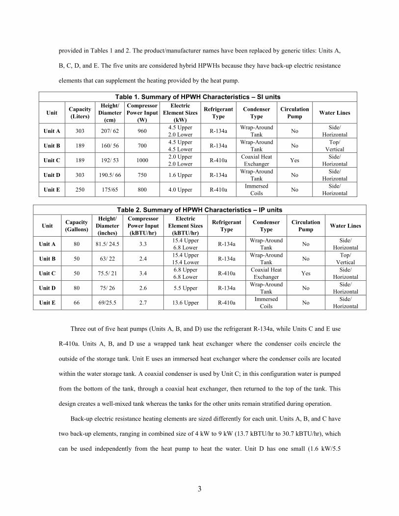
provided in Tables 1 and 2. The product/manufacturer names have been replaced by generic titles: Units A,

B, C, D, and E. The five units are considered hybrid HPWHs because they have back-up electric resistance

elements that can supplement the heating provided by the heat pump.

Table 1. Summary of HPWH Characteristics – SI units

Unit Capacity (Liters)

Height/ Diameter

(cm)

Compressor Power Input

(W)

Electric Element Sizes

(kW)

Refrigerant Type

Condenser Type

Circulation Pump Water Lines

Unit A 303 207/ 62 960 4.5 Upper 2.0 Lower R-134a Wrap-Around

Tank No Side/ Horizontal

Unit B 189 160/ 56 700 4.5 Upper 4.5 Lower R-134a Wrap-Around

Tank No Top/ Vertical

Unit C 189 192/ 53 1000 2.0 Upper 2.0 Lower R-410a Coaxial Heat

Exchanger Yes Side/ Horizontal

Unit D 303 190.5/ 66 750 1.6 Upper R-134a Wrap-Around Tank No Side/

Horizontal

Unit E 250 175/65 800 4.0 Upper R-410a Immersed Coils No Side/

Horizontal

Table 2. Summary of HPWH Characteristics – IP units

Unit Capacity (Gallons)

Height/ Diameter (inches)

Compressor Power Input (kBTU/hr)

Electric Element Sizes

(kBTU/hr)

Refrigerant Type

Condenser Type

Circulation Pump Water Lines

Unit A 80 81.5/ 24.5 3.3 15.4 Upper 6.8 Lower R-134a Wrap-Around

Tank No Side/ Horizontal

Unit B 50 63/ 22 2.4 15.4 Upper 15.4 Lower R-134a Wrap-Around

Tank No Top/ Vertical

Unit C 50 75.5/ 21 3.4 6.8 Upper 6.8 Lower R-410a Coaxial Heat

Exchanger Yes Side/ Horizontal

Unit D 80 75/ 26 2.6 5.5 Upper R-134a Wrap-Around Tank No Side/

Horizontal

Unit E 66 69/25.5 2.7 13.6 Upper R-410a Immersed Coils No Side/

Horizontal

Three out of five heat pumps (Units A, B, and D) use the refrigerant R-134a, while Units C and E use

R-410a. Units A, B, and D use a wrapped tank heat exchanger where the condenser coils encircle the

outside of the storage tank. Unit E uses an immersed heat exchanger where the condenser coils are located

within the water storage tank. A coaxial condenser is used by Unit C; in this configuration water is pumped

from the bottom of the tank, through a coaxial heat exchanger, then returned to the top of the tank. This

design creates a well-mixed tank whereas the tanks for the other units remain stratified during operation.

Back-up electric resistance heating elements are sized differently for each unit. Units A, B, and C have

two back-up elements, ranging in combined size of 4 kW to 9 kW (13.7 kBTU/hr to 30.7 kBTU/hr), which

can be used independently from the heat pump to heat the water. Unit D has one small (1.6 kW/5.5

4

kBTU/hr) electric resistance heating element used to supplement the heat pump but will never operate

independently. Unit E also uses one electric resistance element that is 4kW (13.7 kBTU/hr). This element is

located in the upper half of the water storage tank and can operate independently from the heat pump.

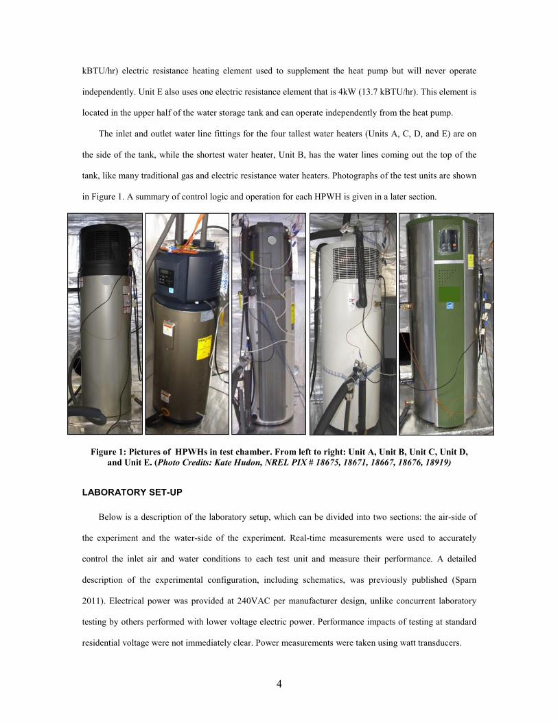
The inlet and outlet water line fittings for the four tallest water heaters (Units A, C, D, and E) are on

the side of the tank, while the shortest water heater, Unit B, has the water lines coming out the top of the

tank, like many traditional gas and electric resistance water heaters. Photographs of the test units are shown

in Figure 1. A summary of control logic and operation for each HPWH is given in a later section.

Figure 1: Pictures of HPWHs in test chamber. From left to right: Unit A, Unit B, Unit C, Unit D, and Unit E. (Photo Credits: Kate Hudon, NREL PIX # 18675, 18671, 18667, 18676, 18919)

LABORATORY SET-UP

Below is a description of the laboratory setup, which can be divided into two sections: the air-side of

the experiment and the water-side of the experiment. Real-time measurements were used to accurately

control the inlet air and water conditions to each test unit and measure their performance. A detailed

description of the experimental configuration, including schematics, was previously published (Sparn

2011). Electrical power was provided at 240VAC per manufacturer design, unlike concurrent laboratory

testing by others performed with lower voltage electric power. Performance impacts of testing at standard

residential voltage were not immediately clear. Power measurements were taken using watt transducers.

5

Test Chamber

The test units were enclosed in a low-mass, insulated air-tight chamber. Two rounds of testing were

completed with two HPWHs tested side-by-side. The units tested were enclosed in the same test chamber

with a physical partition (but not air sealed boundary) to ensure that the operational cycle of one HPWH

did not affect the operation of the other. The two 190 liter (50 gallon) capacity units were tested together,

followed by the two 300 liter (80 gallon) units. Unit E (250 liters/66 gallons) was tested alone.

An inlet duct brought conditioned air to the test chamber, creating a uniform controlled environment

from which the heat pumps drew air. At all times, the chamber’s inlet airflow was greater than the total

airflow used by the HPWHs to allow excess conditioned air to exit the chamber via a bypass duct. As a

result, uniform ambient conditions were ensured in the proximity of each tank. The air flow through the

bypass duct was controlled to a low level to ensure convective heat transfer would not affect tank losses.

Outlet ducting was attached directly to the exhaust of each heat pump so that exit air could be accurately

measured.

Air-Side Equipment

Across the range of tests performed, the air supplied to the test chamber needed to be heated, cooled,

and/or humidified to achieve the desired inlet air conditions. This was accomplished accurately and with

high repeatability using NREL’s Advanced HVAC Systems Laboratory. Test unit inlet air pressure was

averaged across four static pressure taps located in the test chamber.

Each test unit’s exhaust air was collected in an outlet chamber, monitored, and ducted away. Outlet

static pressure taps were located in the outlet chambers. Exhaust air temperature and humidity were

measured in the outlet ducts. Each outlet duct was routed to a laminar flow element (LFE) for accurate

measurement of the airflow rate across the heat pump. Booster fans were used to overcome the pressure

drop of laboratory equipment in the exhaust airstreams, thus preventing the test units from experiencing

any performance-degrading backpressure.

Water-Side Equipment

For each test, a steady and well-controlled inlet water temperature was required. A large holding tank

was pre-conditioned prior to each test and maintained within 0.2°C (0.4°F) of the desired temperature using

6

a resistance heater or chiller with a heat exchanger. Immediately prior to each draw, a valve located close to

each test unit’s inlet was used to fill the inlet piping with water at the desired temperature.

Inlet water temperature and pressure were measured per Federal Register 10 CFR Part 430, Subpart B,

Appendix E (DOE 1998). Inlet and outlet water pipes were insulated to limit heat transfer between the

pipes and their surroundings. The inlet and outlet water flow rates were measured with turbine flow meters.

Heat pump condensate flow rate and density were measured with a coriolis flow meter, and condensate

temperature was measured using an insertion thermocouple.

A thermocouple tree consisting of six thermocouples was placed within each test unit to measure

stratification in the tank. Care was taken to position these thermocouples at the centers of six equal volumes

of water, as prescribed in the above mentioned DOE test specifications document. These measurements

were necessary to calculate the performance of the test units and to help understand their control logic. To

determine if icing was present on the evaporator coils, three surface-mounted thermocouples were installed

on the coils at the inlet, middle, and exit of the evaporator.

For the tests that imposed a prescribed draw profile on the water heaters, an electronically-controlled

proportioning valve was used. The draw profiles were pre-programmed and the turbine flow meter

measurement at the outlet of each test unit was monitored during draws to ensure the correct flow rate.

LABORATORY TESTS AND RESULTS

In order to capture a complete picture of control strategies and realistic performance, four sets of tests

were performed: Standard DOE tests, Operating Mode tests, Draw Profile tests, and Coefficient of

Performance (COP) tests. A description of each test and the results of these tests are given below.

DOE Standard Tests

DOE standard tests are used to provide consumers with a metric for comparing water heaters. The First

Hour Rating (FHR) gives an estimate of the hot water volume that can be provided in a single hour. The

Energy Factor (EF) describes the efficiency of the water heater, taking into account recovery after draws,

standby losses, and cycling losses. We mimicked the DOE tests to ensure the test units were performing as

each manufacturer intended. These tests were run with the units in hybrid mode, except for Unit D, which

does not have multiple operating modes. Standard test methods for both the DOE 1 hour test and 24 hour

7

test were followed per Federal Register 10 CFR Part 430, Subpart B, Appendix E (DOE 1998). Per the test

requirements, the ambient air supplied to the water heaters was 20°C (67.5°F) and 50% relative humidity

(RH). The supply water for the draws was 14°C (58°F).

DOE Test Results. The DOE standard test results and associated calculations will not be discussed in

this paper. More information can be found in our Technical Report (Sparn 2011).

Operating Mode Tests

The operating mode tests were designed to uncover control strategies for each HPWH in all modes of

operation. Before tests began, various sources were used to determine the expected behavior of the units.

Any information that was obtained directly from the manufacturer will be noted in the below descriptions.

Each operating mode test began with the HPWHs at their maximum allowable set point temperature;

the test was later repeated at the recommended 49°C (120°F) set point, if possible. The inlet air temperature

was set at 20°C (67.5°F) dry bulb and 50% RH. The inlet water was controlled to 14°C (58°F). A draw was

initiated and continued until the heat pump turned on (if possible for that mode of operation). The draw was

then stopped and the unit was allowed to recover. A second draw was performed immediately after

recovery for the same air conditions and water heater set point. This second draw continued until the

electric resistance heater(s) came on or until 80% of the tank volume was drawn, whichever occurred first.

The units were then allowed to recover. This process was repeated for all available operating modes.

Detailed results for each manufacturer are presented below and a summary is provided in Table 3.

For hybrid modes of operation, where the heat pump and/or electric resistance heater(s) could be used

to heat the tank, the same process was repeated with cold air (8°C/47°F and 73% RH) and warm air

(35°C/95°F and 40% RH) to determine if air temperature had an effect on the controls. No differences were

observed at these inlet air conditions so the results are not presented in this paper.

8

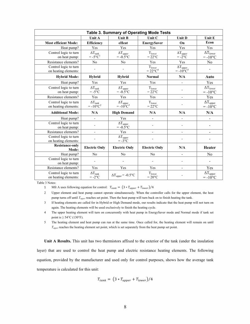
Table 3. Summary of Operating Mode Tests Unit A Unit B Unit C Unit D Unit E

Most efficient Mode: Efficiency eHeat EnergySaver On Econ

Heat pump? Yes Yes Yes Yes Yes Control logic to turn

on heat pump: ΔTtank

= -5°C1 ΔTupper

= -0.5°C Tlower

= 22°C ΔTupper = -2°C

ΔTlower

= -10°C Resistance elements? No No Yes Yes No Control logic to turn on heating elements:

- - Tlower

= 22°C4 ΔTupper

= -10°C5 -

Hybrid Mode: Hybrid Hybrid Normal N/A Auto

Heat pump? Yes Yes Yes - Yes Control logic to turn

on heat pump: ΔTtank = -5°C

ΔTupper = -0.5°C

Tlower = 22°C

- ΔTlower

= -10°C Resistance elements? Yes Yes Yes - Yes Control logic to turn on heating elements:

ΔTtank = -10°C2

ΔTupper = -10°C3

Tlower = 22°C

- ΔTupper

= -10°C

Additional Mode: N/A High Demand N/A N/A N/A

Heat pump? - Yes - - - Control logic to turn

on heat pump: -

ΔTupper = -0.5°C

- - -

Resistance elements? - Yes - - - Control logic to turn on heating elements:

- ΔTupper = -3°C

- - -

Resistance-only Mode:

Electric Only Electric Only Electric Only N/A Heater

Heat pump? No No No - No Control logic to turn

on heat pump: - - - - -

Resistance elements? Yes Yes Yes - Yes Control logic to turn on heating elements:

ΔTtank = -2°C

ΔTupper = -0.5°C Tlower

= 20°C -

ΔTupper

= -10°C Table 3 Notes:

1 Mfr A uses following equation for control: 3 4⁄

2 Upper element and heat pump cannot operate simultaneously. When the controller calls for the upper element, the heat

pump turns off until Tupper reaches set point. Then the heat pump will turn back on to finish heating the tank.

3 If heating elements are called for in Hybrid or High Demand mode, our results indicate that the heat pump will not turn on

again. The heating elements will be used exclusively to finish the heating cycle.

4 The upper heating element will turn on concurrently with heat pump in EnergySaver mode and Normal mode if tank set

point is ≥ 54°C (130°F).

5 The heating element and heat pump can run at the same time. Once called for, the heating element will remain on until

Tupper reaches the heating element set point, which is set separately from the heat pump set point.

Unit A Results. This unit has two thermistors affixed to the exterior of the tank (under the insulation

layer) that are used to control the heat pump and electric resistance heating elements. The following

equation, provided by the manufacturer and used only for control purposes, shows how the average tank

temperature is calculated for this unit: 3 4⁄

9

In this equation, Tupper is the temperature measured by the upper thermistor and Tlower is the temperature

measured by the lower thermistor. The upper thermistor is located near the upper electric resistance heating

element and the lower thermistor is located near the lower electric resistance heating element.

As determined by our experimental results, none of the heat sources – heat pump, upper element, or

lower element – operate concurrently. Also, if the tank temperature is below 14°C (58°F) at initial start up,

the heat pump will not run and the upper heating element will turn on instead.

1. Efficiency Mode:

2.

The heat pump turns on when Ttank drops 5°C (9°F) below the set point temperature

and runs until Ttank reaches set point. The heat pump is used exclusively unless the air temperature is

outside the operating bounds defined by the manufacturer (7°C/45°F to 43°C/109°F), or Ttank falls

below 14°C (58°F). For these conditions, the upper heating element turns on until Tupper reaches set

point. This mode is expected to meet the hot water demand for most households. The heat pump turns

on before the hot water is depleted, thus maximizing the volume of hot water delivered to the end user.

Hybrid Mode:

3.

The heat pump will turn on when a 5°C (9°F) drop in Ttank is detected and the upper

heating element will turn on, in place of the heat pump, when Ttank has dropped by 10°C (18°F). The

upper element will turn off when Tupper is at set point and revert to the heat pump to finish the heating

cycle. This mode is the best choice for high demand situations since the top of the tank will be

maintained by the upper heating element while maximizing the use of the heat pump when possible.

Electric Only Mode:

Unit B Results. This HPWH does not allow the two electric resistance heating elements to operate

simultaneously or alongside the heat pump. A thermistor located near the upper heating element is used to

control the heating logic for this unit. This information was provided by the manufacturer.

Electric resistance heating elements will be used to heat the tank. A small drop in

Ttank (2°C/4°F) will cause the upper heating element to turn on. The upper element will remain on until

Tupper is at set point. The lower element will then turn on to heat the rest of the tank. Because the lower

heating element has a small heating capacity (2kW/6.8kBtu/hr), this mode showed no improvement

over Hybrid mode in delivered hot water volume, recovery time, or efficiency. This mode should only

be used when the heat pump is not operating correctly.

1. eHeat Mode: The heat pump will turn on once a small temperature drop (0.5°C/1°F) is detected by the

thermistor. This mode uses the heat pump exclusively unless the air temperature is outside the

10

operating bounds defined by the manufacturer (7°C/45°F to 49°C/120°F). A heating element will turn

on when icing occurs on the evaporator coils. This mode is very efficient, but tank recovery is slow

due to the heating capacity of the compressor. This mode is ideal for low demand situations.

2. Hybrid Mode:

3.

Similar to eHeat mode, the heat pump will turn on once a small drop in temperature is

measured by the thermistor. A more significant drop in temperature (10°C/18°F) will cause a heating

element to turn on. The lower heating element turns on first for moderately large draws and the upper

element turns on first for very large draws. If the lower element turns on first, it will heat the tank to

the set point temperature without using the upper element. If the upper element turns on first, it will

remain on until the thermistor at the top of tank reads a temperature 3°C (5°F) below the set point

temperature. The lower element will then turn on. Once an electric element turns on, we observed that

the heat pump will not be used for the remainder of the heating cycle. It should be noted that the

manufacturer claims that the heat pump will turn back on in some situations. This mode is good for

moderate demand situations, but there will be a significant reduction in efficiency if the heating

elements are enabled.

High Demand Mode:

4.

This mode is very similar to Hybrid mode, but the electric elements will turn on

sooner than in Hybrid mode, when the temperature at the thermistor drops 3°C (5°F). This mode is

recommended for high demand situations, but significantly reduces the efficiency of the unit.

Electric Only Mode:

Unit C Results. The heat pump and upper heating element, or both heating elements, can run

concurrently. A thermistor located near the lower element is used to trigger the operation of the heat pump

and/or heating elements. A second thermistor located near the upper element determines when the heat

pump or heating elements turn off. If the water in the tank is below 27°C (80°F) at initial start up, the heat

pump will not run and the upper element will be used until the temperature exceeds 27°C (80°F). This

The upper heating element will turn on when the temperature at the thermistor

drops 0.5°C (1°F) and will heat until the top of the tank is 3°C (5°F) below set point. The lower

element is used to heat the lower half of the tank. The lower element will turn off when the thermistor

near the top of the tank reads the set point temperature. This mode offers quick recovery, but is the

least efficient operating mode.

11

restriction only applies when the power to the unit is turned on, and does not apply during a draw event.

This information was provided by the manufacturer and confirmed during testing.

1. Energy Saver Mode:

• Even though the user manual states that the heat pump will operate in air temperatures between

4°C (40°F) and 49°C (120°F), we did not see continuous operation of the heat pump for air

temperatures below 14°C (57°F) or above 35°C (95°F). For air temperatures below 14°C (57°F),

icing occurred on the evaporator coils. This caused the heat pump to cycle on and off three times

before switching to resistance heat for the remainder of the heating cycle. Above 35°C (95°F) the

heat pump cycled on once before switching to the heating elements. It is believed that system

optimization and redesign would extend the operating range of this unit.

The heat pump turns on when the thermistor located near the lower heating

element reads a temperature around 22°C (76°F). The heat pump operates alone if the water

temperature set point is 52°C (125°F) or below, unless the air temperature is outside the manufacturer

stated operating bounds (4°C/40°F and 49°C/120°F). When the set point is at its highest (58°C/136°F),

the heat pump and upper element are used primarily, and they always operate together at the end of the

heating cycle. The use of the heat pump alone versus the use of the heat pump and upper element

appears to be tied to the set point temperature, rather than draw size. The two heating elements will not

operate without the heat pump in this mode, unless the air temperature is outside the acceptable

bounds. Our test results indicate that this system is limited in its operating range, as described below.

This mode is efficient, quick to recover, and should be used as the primary operating mode.

2. Normal Mode:

3.

This mode is very similar to the Energy Saver mode. For a 49°C (120°F) tank set point,

the heat pump will turn on alone, except at the very end of the heating cycle when the upper heating

element will also be used. For the highest set point (58°C/135°F), the heat pump and upper heating

element turn on. The temperature trigger for the heat pump is the same as in Energy Saver mode. There

is no apparent advantage to this operating mode compared to the Energy Saver mode.

Electric Only Mode: Both heating elements will turn on when the thermistor temperature drops to

20°C (68°F) but the lower element will turn on first, after a small drop in temperature (~0.5°C/1°F) is

detected by the lower thermistor. The upper element will turn off when the top of the tank has reached

set point and the lower element will remain on to heat the lower half of the tank.

12

Unit D Results. A single thermistor, located at the top of the tank, is used to control heating for this

water heater. There is only one operating mode for this unit. The heat pump can operate at the same time as

the electric resistance element, but the electric element cannot run on its own.

1. On:

Unit E Results. Two thermistors are used to control the heating logic for this unit. According to the

manufacturer, the lower thermistor is located at roughly the mid-point of the tank. The upper thermistor is

located near the heating element and is half way between the top of the tank and the lower thermistor. The

lower thermistor controls the heat pump and the upper thermistor controls the heating element. The heat

pump and heating element can operate simultaneously. It should be noted that the unit tested was a pre-

production unit. Therefore, the results presented here might differ if compared to the production version.

The heat pump will turn on when the thermistor registers a small drop in temperature (2°C/4°F)

from set point. The heating element will turn on when the top of the tank drops 10°C (18°F) below set

point. When the draw is large enough to trigger the heating element, it will remain on until the

thermistor reaches the heating element set point. The default set point is 55°C (131°F), which is below

the default heat pump set point of 60°C (140°F). The rest of the tank will be heated with the heat pump

until the thermistor reading reaches the heat pump set point. According to the user manual, the

operating range for this unit is between air temperatures of 6°C (43°F) and 42°C (107°F).

1. Econ Mode:

• A timer period must be defined by the user for the heat pump to operate in this mode.

The heat pump will turn on when the lower thermistor measures a temperature 10-15°C

(18-27°F) below the set point. The heat pump will turn off when the lower thermistor returns to the set

point. The deadband, which is 5°C (10°F) according to the manufacturer, can be adjusted by the user

through the user interface. Our results indicate that the deadband is larger than expected. At a set point

of 49°C (120°F), a 10°C (18°F) drop in temperature at the lower thermistor caused the heat pump to

turn on, and at the 57°C (135°F) set point, a 15°C (27°F) drop was required for heat pump operation.

Even though a relatively large draw is required to trigger the heat pump, its heating capacity is large

enough to recover the tank quickly. Other items to note:

• If icing occurs on the coils, the fan turns off for two minutes and a refrigerant reversal valve is

used to reverse the flow of refrigerant in the heat pump. The heat pump then runs normally for 20

minutes and this process is repeated again if needed.

13

This mode is efficient and should be used for households with a small to moderate hot water demand.

2. Auto Mode:

3.

As with Econ Mode, the heat pump will turn on once the lower thermistor measures a

temperature drop from set point of 10-15°C (18-27°F). The resistance heater will turn on when the

upper thermistor measures a drop in temperature of 10-20°C (18-36°F) and will turn off when the

upper thermistor is at set point. If the resistance heater is called for, the heat pump will remain on and

continue to heat the tank until the lower thermistor reaches set point. Unlike Econ Mode, a timer

period does not need to be set to operate the heat pump. This mode should provide sufficient hot water

for all users, including high demand households.

Heater Mode:

Draw Profile Tests

This mode will use the resistance heating element to heat the tank. Similar to Auto

Mode, the resistance heater will turn on when a drop in temperature of 10-20°C (18-36°F) degrees is

detected by the upper thermistor. The electric element is located in the upper third of the tank, so in

Heater Mode, only the top third of the tank will be heated. This mode will not satisfy hot water

demands for most users and should not be used as the primary heating mode.

Two draw profiles were used to challenge the HPWHs with high volume draws and repeated low

volume draws. A tabular representation of each draw profile can be found in Tables 4 and 5. Each test

began with the water heaters at a set point of 49°C (120°F), operating in hybrid mode. The supply water

temperature for these tests was 7°C (45°F). Draw Profile 1 contained a ‘morning’ and an ‘evening’

segment. After the morning draws were complete, the units were allowed to recover and sit idle for

approximately five minutes before starting the evening segment. Draw Profile 2 consisted of many short

draws and was allowed to run uninterrupted.

Draw Profile Results. The morning segment of Draw Profile 1 simulated four shower draws over the

course of about an hour. The two HPWHs with the smallest storage tanks were unable to provide hot water

for all four showers. The outlet temperature for Unit B dropped below our standard for “hot” water

(40.5°C/105°F) during the third shower and the coldest delivered temperature during the fourth shower was

28°C (82°F). This hot water standard was taken from the Building America House Simulation Protocols

document (NREL 2010), which was revised to a “hot” water standard of 43.3°C (110°F) after our testing

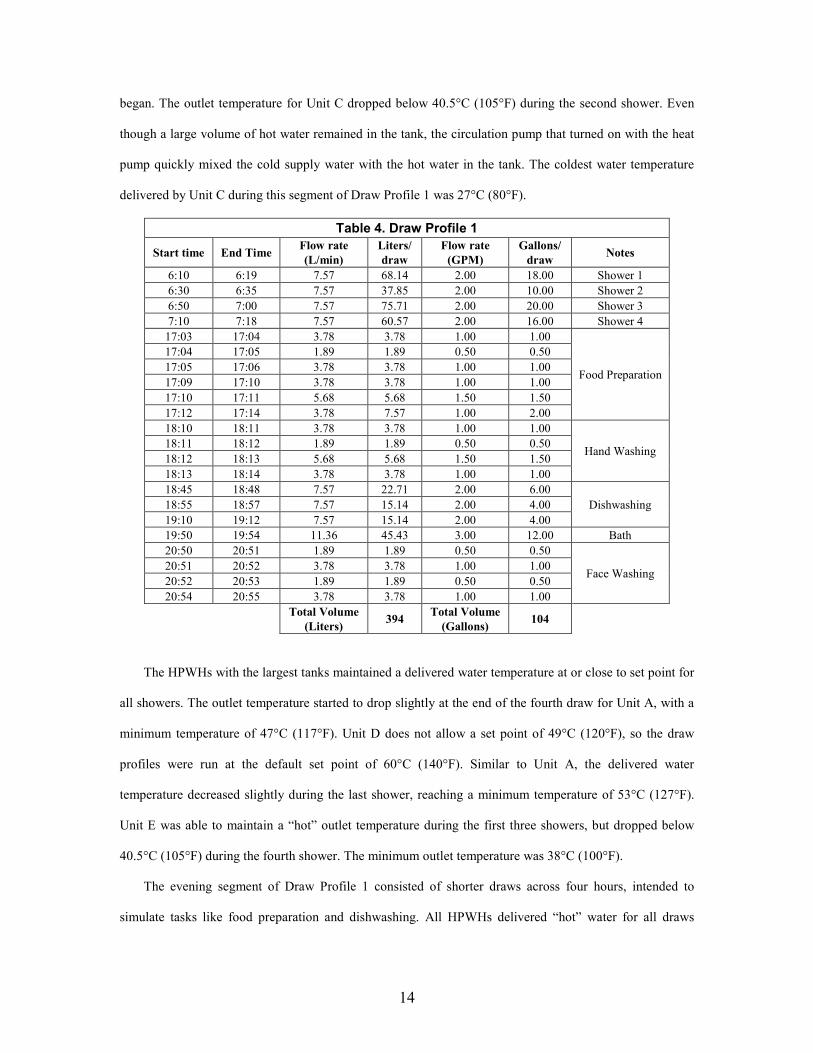
14

began. The outlet temperature for Unit C dropped below 40.5°C (105°F) during the second shower. Even

though a large volume of hot water remained in the tank, the circulation pump that turned on with the heat

pump quickly mixed the cold supply water with the hot water in the tank. The coldest water temperature

delivered by Unit C during this segment of Draw Profile 1 was 27°C (80°F).

Table 4. Draw Profile 1

Start time End Time Flow rate (L/min)

Liters/draw

Flow rate (GPM)

Gallons/draw Notes

6:10 6:19 7.57 68.14 2.00 18.00 Shower 1 6:30 6:35 7.57 37.85 2.00 10.00 Shower 2 6:50 7:00 7.57 75.71 2.00 20.00 Shower 3 7:10 7:18 7.57 60.57 2.00 16.00 Shower 4

17:03 17:04 3.78 3.78 1.00 1.00

Food Preparation

17:04 17:05 1.89 1.89 0.50 0.50 17:05 17:06 3.78 3.78 1.00 1.00 17:09 17:10 3.78 3.78 1.00 1.00 17:10 17:11 5.68 5.68 1.50 1.50 17:12 17:14 3.78 7.57 1.00 2.00 18:10 18:11 3.78 3.78 1.00 1.00

Hand Washing 18:11 18:12 1.89 1.89 0.50 0.50 18:12 18:13 5.68 5.68 1.50 1.50 18:13 18:14 3.78 3.78 1.00 1.00 18:45 18:48 7.57 22.71 2.00 6.00

Dishwashing 18:55 18:57 7.57 15.14 2.00 4.00 19:10 19:12 7.57 15.14 2.00 4.00 19:50 19:54 11.36 45.43 3.00 12.00 Bath 20:50 20:51 1.89 1.89 0.50 0.50

Face Washing 20:51 20:52 3.78 3.78 1.00 1.00 20:52 20:53 1.89 1.89 0.50 0.50 20:54 20:55 3.78 3.78 1.00 1.00

Total Volume (Liters) 394 Total Volume

(Gallons) 104

The HPWHs with the largest tanks maintained a delivered water temperature at or close to set point for

all showers. The outlet temperature started to drop slightly at the end of the fourth draw for Unit A, with a

minimum temperature of 47°C (117°F). Unit D does not allow a set point of 49°C (120°F), so the draw

profiles were run at the default set point of 60°C (140°F). Similar to Unit A, the delivered water

temperature decreased slightly during the last shower, reaching a minimum temperature of 53°C (127°F).

Unit E was able to maintain a “hot” outlet temperature during the first three showers, but dropped below

40.5°C (105°F) during the fourth shower. The minimum outlet temperature was 38°C (100°F).

The evening segment of Draw Profile 1 consisted of shorter draws across four hours, intended to

simulate tasks like food preparation and dishwashing. All HPWHs delivered “hot” water for all draws

15

except Unit B, whose outlet temperature dipped below 40.5°C (105°F) during an extended draw near the

end of the evening segment. All subsequent draws were satisfied with “hot” water.

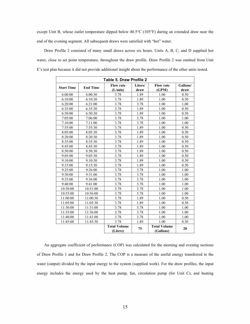
Draw Profile 2 consisted of many small draws across six hours. Units A, B, C, and D supplied hot

water, close to set point temperature, throughout the draw profile. Draw Profile 2 was omitted from Unit

E’s test plan because it did not provide additional insight about the performance of the other units tested.

Table 5. Draw Profile 2

Start Time End Time Flow rate (L/min)

Liters/draw

Flow rate (GPM)

Gallons/draw

6:00:00 6:00:30 3.78 1.89 1.00 0.50 6:10:00 6:10:30 3.78 1.89 1.00 0.50 6:20:00 6:21:00 3.78 3.78 1.00 1.00 6:35:00 6:35:30 3.78 1.89 1.00 0.50 6:50:00 6:50:30 3.78 1.89 1.00 0.50 7:05:00 7:06:00 3.78 3.78 1.00 1.00 7:10:00 7:11:00 3.78 3.78 1.00 1.00 7:55:00 7:55:30 3.78 1.89 1.00 0.50 8:05:00 8:05:30 3.78 1.89 1.00 0.50 8:20:00 8:20:30 3.78 1.89 1.00 0.50 8:35:00 8:35:30 3.78 1.89 1.00 0.50 8:45:00 8:45:30 3.78 1.89 1.00 0.50 8:50:00 8:50:30 3.78 1.89 1.00 0.50 9:05:00 9:05:30 3.78 1.89 1.00 0.50 9:10:00 9:10:30 3.78 1.89 1.00 0.50 9:15:00 9:15:30 3.78 1.89 1.00 0.50 9:25:00 9:26:00 3.78 3.78 1.00 1.00 9:30:00 9:31:00 3.78 3.78 1.00 1.00 9:35:00 9:36:00 3.78 3.78 1.00 1.00 9:40:00 9:41:00 3.78 3.78 1.00 1.00

10:50:00 10:51:00 3.78 3.78 1.00 1.00 10:55:00 10:56:00 3.78 3.78 1.00 1.00 11:00:00 11:00:30 3.78 1.89 1.00 0.50 11:05:00 11:05:30 3.78 1.89 1.00 0.50 11:30:00 11:31:00 3.78 3.78 1.00 1.00 11:35:00 11:36:00 3.78 3.78 1.00 1.00 11:40:00 11:41:00 3.78 3.78 1.00 1.00 11:45:00 11:45:30 3.78 1.89 1.00 0.50

Total Volume (Liters) 75 Total Volume

(Gallons) 20

An aggregate coefficient of performance (COP) was calculated for the morning and evening sections

of Draw Profile 1 and for Draw Profile 2. The COP is a measure of the useful energy transferred to the

water (output) divided by the input energy to the system (supplied work). For the draw profiles, the input

energy includes the energy used by the heat pump, fan, circulation pump (for Unit C), and heating

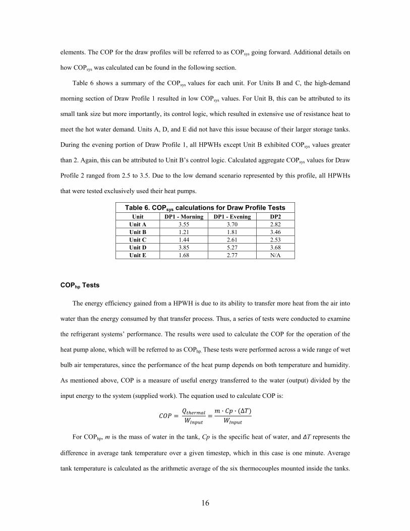
16

elements. The COP for the draw profiles will be referred to as COPsys going forward. Additional details on

how COPsys was calculated can be found in the following section.

Table 6 shows a summary of the COPsys values for each unit. For Units B and C, the high-demand

morning section of Draw Profile 1 resulted in low COPsys values. For Unit B, this can be attributed to its

small tank size but more importantly, its control logic, which resulted in extensive use of resistance heat to

meet the hot water demand. Units A, D, and E did not have this issue because of their larger storage tanks.

During the evening portion of Draw Profile 1, all HPWHs except Unit B exhibited COPsys values greater

than 2. Again, this can be attributed to Unit B’s control logic. Calculated aggregate COPsys values for Draw

Profile 2 ranged from 2.5 to 3.5. Due to the low demand scenario represented by this profile, all HPWHs

that were tested exclusively used their heat pumps.

Table 6. COPsys calculations for Draw Profile Tests Unit DP1 - Morning DP1 - Evening DP2

Unit A 3.55 3.70 2.82 Unit B 1.21 1.81 3.46 Unit C 1.44 2.61 2.53 Unit D 3.85 5.27 3.68 Unit E 1.68 2.77 N/A

COPhp Tests

The energy efficiency gained from a HPWH is due to its ability to transfer more heat from the air into

water than the energy consumed by that transfer process. Thus, a series of tests were conducted to examine

the refrigerant systems’ performance. The results were used to calculate the COP for the operation of the

heat pump alone, which will be referred to as COPhp. These tests were performed across a wide range of wet

bulb air temperatures, since the performance of the heat pump depends on both temperature and humidity.

As mentioned above, COP is a measure of useful energy transferred to the water (output) divided by the

input energy to the system (supplied work). The equation used to calculate COP is:

· · ∆

For COPhp, m is the mass of water in the tank, Cp is the specific heat of water, and ΔT represents the

difference in average tank temperature over a given timestep, which in this case is one minute. Average

tank temperature is calculated as the arithmetic average of the six thermocouples mounted inside the tanks.

17

The supplied work consists of the input energy from the heat pump, fan, and circulation pump, if

applicable. This energy was measured as the overall input to the water heater and is represented by WInput.

For the COPsys calculations mentioned previously, m is the mass of the volume drawn (determined

using the volume flow rate) and ΔT is the difference between the outlet and inlet water temperatures during

draws. The supplied work term also includes Welements, which is the work provided by the electric heating

elements. The stand-by losses are not incorporated into the COPsys calculation because the inlet and outlet

water temperatures are used to calculate the thermal energy instead of changes in the average tank

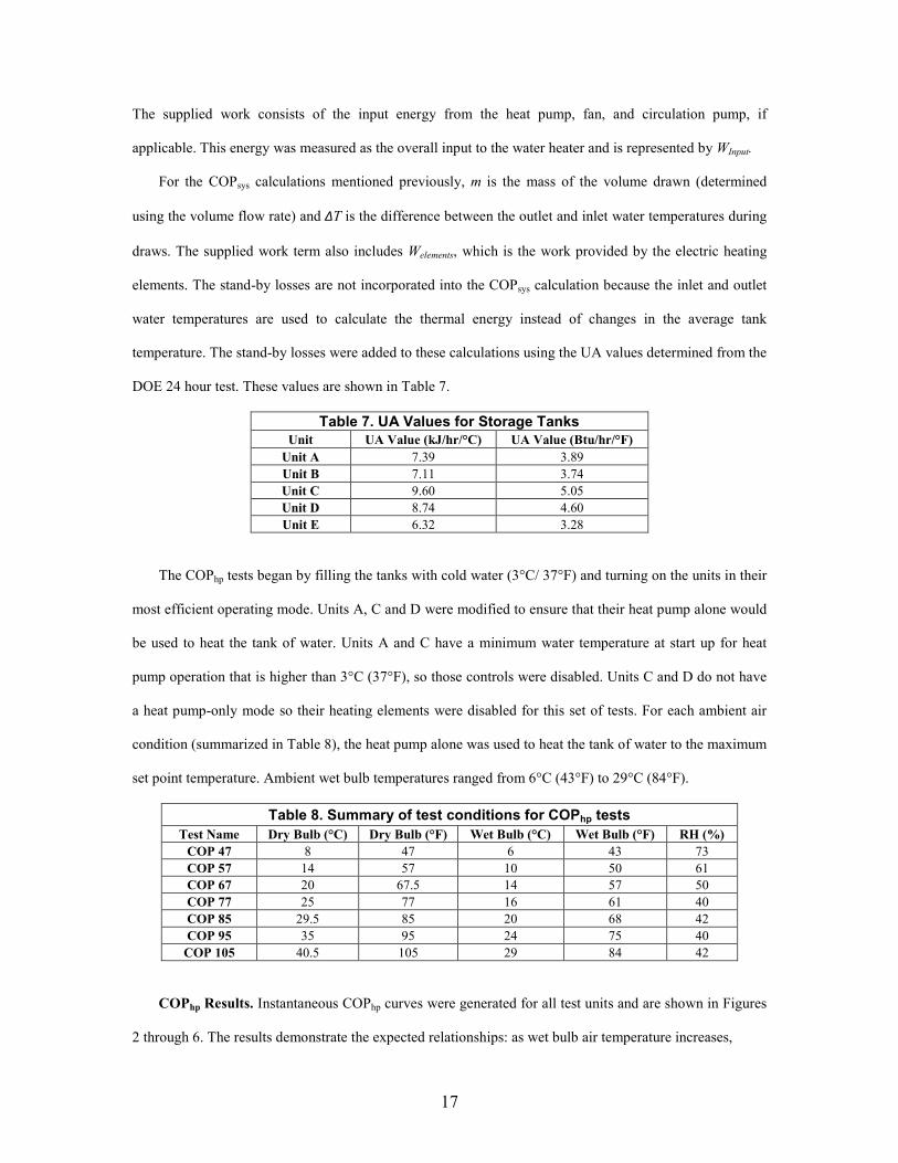
temperature. The stand-by losses were added to these calculations using the UA values determined from the

DOE 24 hour test. These values are shown in Table 7.

Table 7. UA Values for Storage Tanks Unit UA Value (kJ/hr/°C) UA Value (Btu/hr/°F)

Unit A 7.39 3.89 Unit B 7.11 3.74 Unit C 9.60 5.05 Unit D 8.74 4.60 Unit E 6.32 3.28

The COPhp tests began by filling the tanks with cold water (3°C/ 37°F) and turning on the units in their

most efficient operating mode. Units A, C and D were modified to ensure that their heat pump alone would

be used to heat the tank of water. Units A and C have a minimum water temperature at start up for heat

pump operation that is higher than 3°C (37°F), so those controls were disabled. Units C and D do not have

a heat pump-only mode so their heating elements were disabled for this set of tests. For each ambient air

condition (summarized in Table 8), the heat pump alone was used to heat the tank of water to the maximum

set point temperature. Ambient wet bulb temperatures ranged from 6°C (43°F) to 29°C (84°F).

Table 8. Summary of test conditions for COPhp tests Test Name Dry Bulb (°C) Dry Bulb (°F) Wet Bulb (°C) Wet Bulb (°F) RH (%)

COP 47 8 47 6 43 73 COP 57 14 57 10 50 61 COP 67 20 67.5 14 57 50 COP 77 25 77 16 61 40 COP 85 29.5 85 20 68 42 COP 95 35 95 24 75 40

COP 105 40.5 105 29 84 42

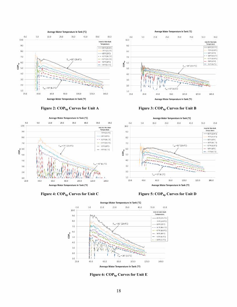
COPhp Results. Instantaneous COPhp curves were generated for all test units and are shown in Figures

2 through 6. The results demonstrate the expected relationships: as wet bulb air temperature increases,

18

Figure 2: COPhp Curves for Unit A Figure 3: COPhp Curves for Unit B

Figure 4: COPhp Curves for Unit C Figure 5: COPhp Curves for Unit D

Figure 6: COPhp Curves for Unit E

19

COPhp increases, and as average tank temperature increases, COPhp decreases. The oscillating lines at low

air temperatures represent the heat pump cycling off and on due to icing on the evaporator coils.

Beginning with a full tank of cold water, the highest COPhp values range between 3.5 at the coldest wet

bulb temperature and 7 at the highest wet bulb temperature. At the highest average water temperatures,

COPhp generally ranged between 2 and 4 for the lowest and highest wet bulb temperatures, respectively.

One noticeable difference between the five units is that Unit C achieved complete COPhp curves for

only four inlet air conditions. This is because the two coldest air conditions caused icing on the coils that

prohibited continuous heat pump operation and the warmest air condition caused the heat pump to turn off

in favor of the electric resistance elements. It is believed this occurred because the system capacity and

condenser design is not optimized for low or high air temperatures. This limitation occurred despite the fact

that all air conditions tested were within the operating range as stated by the manufacturer. It should be

noted that at inlet air conditions within its measured operating range, Unit C performed well.

The COPhp curves also show that, despite small differences between units, all test units operate

efficiently (COPhp > 1.5) over the range of conditions tested. Excluding Unit C, all test units provided

efficient water heating at relatively cold air temperatures, as compared to other methods of water heating.

TECHNOLOGY STRENGTHS AND SHORTFALLS BASED ON TEST RESULTS

Physically, these water heaters present new considerations for homeowners at installation. All units are

taller than traditional water heaters and the 300 liter (80 gallon) units are significantly taller. Airflow

requirements vary between units, but Unit A draws significantly more air (0.24 m3/s, 500 cfm) compared to

the other units tested which draw between 0.05 – 0.10 m3/s (100-200 cfm). Also, Units A, C, D, and E have

side-mounted water connections, meaning that additional plumbing may be required for retrofit

installations. Installation location must be considered by a homeowner before purchasing a unit.

The units with smaller tanks demonstrated difficulty in maintaining hot water delivery in high demand

situations, even if their electric resistance elements are used. The units with larger tanks provide a buffer in

times of high demand and therefore are expected to use their heat pump for recovery, rather than reverting

to electric resistance heating to maintain outlet temperature. The result is more efficient operation and

20

better performance in terms of availability of hot water. In households with more than two occupants, a

HPWH with a larger tank will likely be a better option.

The coaxial condenser used by Unit C relies on a circulation pump for heat transfer to the tank of

water, which creates a well-mixed tank. If the heat pump is turned on during a draw, the cold inlet water is

mixed with the hot water in the tank, causing the outlet water temperature to drop. This also causes the

upper element to cycle on. In contrast, the wrapped tank condenser design allows for efficient heat transfer

between the refrigerant system and the water without incorporating a circulation pump. This helps maintain

tank stratification since the cold inlet water stays at the bottom of the tank and hot water is drawn from the

top of the tank. This stratification results in a higher sustained outlet water temperature.

Three of the HPWHs use the refrigerant R134a in their heat pumps, while two test units use R410a.

One of the main differences between these two refrigerants is their critical points. Critical point for R410a

is 70.22°C (158.4°F) (ASHRAE 2009). It is not clear why one unit using R410a operated well across the

range of conditions tested, whereas another demonstrated a limited performance range. This is indicative of

early versions of a new technology, and points to an opportunity for greater efficiency in future designs.

The recovery rate for HPWH technology is a concern because it takes longer to heat water using a heat

pump than it does using electric resistance heating elements. In addition, there are differences between

recovery rates for the various manufacturers because of the different capacities of their compressors.

Table 9. Recovery Rate Comparison at 14°C (57°F) Inlet Wet Bulb Air Temperature – Heat Pump vs. Electric

Unit Recovery Rate (°C/hour)

Recovery Rate (°F/hour)

Percent Reduction vs. Electric (%)

Unit A 8.5 15.3 61.9 Unit B 6.3 11.4 71.8 Unit C 13.2 23.7 40.8 Unit D 5.4 9.7 75.8 Unit E 9.6 17.3 57.0

Electric WH with 4.5kW (15kBTU/h) capacity (Energy Plus)

(50 Gallon/189 Liter) 22.3 40.2 0.0

Table 9 shows recovery rate in degrees per hour for each test unit at an inlet wet bulb temperature of

14°C (57°F). These values represent recovery rates during heat pump operation, without the assistance of

heating elements, and are consistent with the nominal power inputs for each unit (within 2%). Unit C has

the highest recovery rate and Unit D has the lowest. Relative to a typical 4.5kW (15kBTU/h) electric

21

resistance water heater, this represents a 41% and 76% decrease in recovery rate, respectively. Although

this may appear significant to a homeowner, the negative impact of a slower recovery rate can be mitigated

by installing a unit with a larger storage tank.

Control logic and component sizing have a significant impact on the overall performance of the units

tested, both in terms of energy efficiency and hot water delivery. The units with two tank thermistors, Units

A, C, and E, used the lower thermistor to cue the operation of the heat pump. That allows the heat pump to

start recovery after a small draw and helps to avoid using the heating elements in response to a large draw.

In contract, Unit D uses a single thermistor located at the top of the tank to control the heat pump. By the

time the thermistor registers a temperature drop, 75% of the tank (225 liters/60 gallons) has been drained

and refilled with cold water. In addition, the heating capacities of the heat pump and the resistance element

are small, resulting in a slow recovery rate. Modifications to the control logic and component sizes for this

unit could result in significant improvements in system performance.

Units C, D and E have resistance elements small enough to run concurrently with the heat pump and

therefore have more options for control. For Unit C’s maximum set point temperature, the upper element

and heat pump will run together for the entire heating cycle, which speeds the recovery time considerably.

Unit D only uses its electric element to bring the very top of the tank to set point but that creates available

hot water quickly. Units A and B do not run their electric elements with the heat pump. If demand on Unit

B is large enough to trigger the electric resistance elements, we observed that the heat pump will not turn

back on during that heating cycle, which means recovery will be fast, but inefficient. Unit A uses its large

upper resistance element to quickly heat the top of the tank to set point before reverting back to the heat

pump alone to finish heating the tank. Control logic is key to HPWH efficiency and performance and is

expected to be optimized in future generations of these units.

Accessibility to the airflow filter varied in the test units. Easy access to the filter is essential so that

homeowners can clean the filter as needed. Units A, B, and C have filters that are easily accessible. Unit D

does not have an airflow filter, and the pre-production Unit E has a filter that is not easily accessible.

All of these units are more expensive than traditional electric resistance water heaters, with the smaller

units priced around $1500 and the larger units selling for $2200 and up. However, if sized properly for

household needs and operated correctly, heat pump water heaters have the potential to significantly reduce

22

electricity bills for homes using standard electric resistance water heaters. The climate and the location

within the home (conditioned space or unconditioned space) will impact the actual savings. If a heat pump

water heater is located inside the home’s conditioned space, it will interact with the heating and cooling

system in a way that may or may not benefit the homeowners. Extensive whole-house modeling is used to

explore these building interactions and the impact of HPWHs across US climate regions. Simulations can

provide insight into the technology’s expected lifetime costs and energy savings potential.

HEAT PUMP WATER HEATER MODEL FOR WHOLE-HOUSE ENERGY SIMULATIONS

A key motivation for the HPWH laboratory tests was to obtain data for model validation. A valid

model should represent the family of HPWHs currently available on the market, and be incorporated into

annual whole-house simulation tools. These tools simulate the interactions of residential building

components as an integrated system, thus accounting for the HPWH cooling in context of the whole

building. Such an annual energy simulation is essential for validating this emerging technology and could

help determine the expected energy savings for HPWHs in any climate region, when installed in either a

conditioned or unconditioned space.

ENERGYPLUS HPWH MODEL DESCRIPTION AND VALIDATION

A HPWH model exists in the energy simulation software, EnergyPlus V.6.0.0 (EnergyPlus 2010). This

model was developed to represent commercial building HPWH technology, so the configuration differs in

terms of the physical characteristics and control logic compared to the integrated HPWHs we tested. The

first step in modeling the current class of residential HPWHs was to evaluate this existing model using the

laboratory data and determine if it represents the above mentioned HPWH units.

The EnergyPlus HPWH model represents a combination of components that already exist in

EnergyPlus. It combines a well-mixed, isothermal electric resistance water tank, a direct expansion (DX)

system that is located external to the water tank, and a fan. The DX system model includes an evaporator,

compressor, condenser, and water circulation pump that operate together. The fan moves surrounding air

across the evaporator coil such that heat is absorbed into the refrigerant. This refrigerant is then

compressed, increasing its temperature, and this heat it then transferred to the water via the condenser coil.

23

One major configuration difference between the model and the majority of integrated HPWHs

currently available is that the model assumes water from the storage tank is pumped to an external

condensing heat exchanger, which can create a fully-mixed water tank, depending on flow rates. While this

physical configuration is consistent with Unit C, it is not representative of the other available HPWHs on

the market. This model assumes the heat pump is the primary heating source but is configured with back-up

electric resistance elements in high-demand situations, which is representative of the units tested.

The HPWH data that was chosen for this validation was from Unit B, since the control logic for this

unit was the easiest to model given the current capabilities of EnergyPlus and the configuration of this unit

is the most representative of the family of heat pump water heaters that are currently available. Using the

data from this unit, biquadratic curves representing the compressor heating capacity and heat pump COP

were created. These curves were defined using the following equation,

where Twb is the inlet air wet bulb temperature and Twa is the average water temperature in the storage tank.

The coefficients used to define COPhp and heating capacity for Unit B can be found in Table 10. The COPhp

and heating capacity equations were normalized by rated COPhp and rated heating capacity, respectively.

The rated COPhp for Unit B is 2.76 and the rated heating capacity is 1.4 kW (4.7 kBtu/hr). The rated

conditions are defined at a Twb of 14°C (57°F) and a Twa of 48.9°C (120°F). It should be noted that these

equations do not take into account stand-by tank losses. Stanby-by losses must be accounted for in the

simulation using the UA values in Table 7.

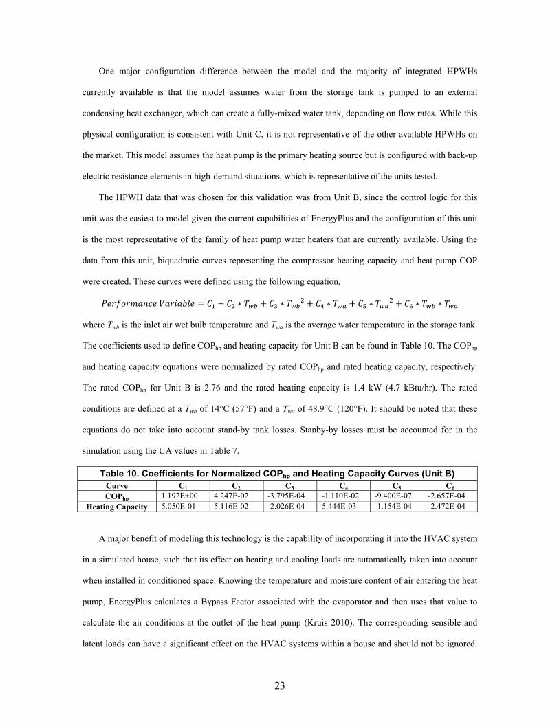
Table 10. Coefficients for Normalized COPhp and Heating Capacity Curves (Unit B) Curve C1 C2 C3 C4 C5 C6 COPhp 1.192E+00 4.247E-02 -3.795E-04 -1.110E-02 -9.400E-07 -2.657E-04

Heating Capacity 5.050E-01 5.116E-02 -2.026E-04 5.444E-03 -1.154E-04 -2.472E-04

A major benefit of modeling this technology is the capability of incorporating it into the HVAC system

in a simulated house, such that its effect on heating and cooling loads are automatically taken into account

when installed in conditioned space. Knowing the temperature and moisture content of air entering the heat

pump, EnergyPlus calculates a Bypass Factor associated with the evaporator and then uses that value to

calculate the air conditions at the outlet of the heat pump (Kruis 2010). The corresponding sensible and

latent loads can have a significant effect on the HVAC systems within a house and should not be ignored.

24

For example, at the rated conditions given above, Unit B had a sensible cooling capacity of 0.67 kW (0.2

tons of refrigeration) and a sensible heat ratio of 0.875.

The existing EnergyPlus V.6.0.0 HPWH model was used to simulate a draw profile to determine if the

model matches the experimental results for integrated residential HPWH products. Draw Profile 1 from our

laboratory experiment was modeled, representing the ‘morning’ and ‘evening’ portions of a day. The total

volume of water drawn was 380 liters (~100 gallons) to represent a moderately high-use family.

Simulation results are shown in Figure 7. These figures show the draw profile, HPWH power

consumption, and average tank temperature. The electric power results were used to calculate the energy

use associated with this draw profile. Based on this calculation, it was determined that the current

EnergyPlus model underpredicts HPWH energy use by ~18% when compared to measured data.

Figure 7: EnergyPlus HPWH model results compared to laboratory data for Unit B.

There are several important limitations of the code that must be addressed before using it with

confidence. These limitations are as follows:

• The model assumes a fully-mixed water tank and does not represent the design of Unit B, which

operates with a stratified tank. Consequently, the operation of the HPWH is controlled using average

25

tank temperature, and therefore, it is not possible to simulate product control algorithms that dictate

operation of the heat pump and electric resistance elements. (Note: This means that the deadband

temperature is also based on average tank temperature, and had to be set at a lower temperature than on

the product, in order to better match the data from the draw profile. Although this does not affect the

outcome of the above comparison, it would affect annual simulation results, since stand-by losses

would not be compensated for during long periods without draws. Further, the deadband adjustment is

not easy to predict without unit performance data, combined with trial-and-error.)

• This model overpredicts average tank temperature in high-demand situations. This is also the result of

the model using average tank temperature instead of more realistic stratified temperatures. When draws

are modeled, the outlet temperature of the water is the average temperature of the tank. In reality, the

outlet water temperature will be the hottest temperature in the tank. This difference results in higher

average tank temperatures in the model, thus the energy needed to reheat the water is underpredicted.

• Control logic options for the existing model are limited. For this comparison, modifications were made

to the control logic in the existing model in order to better match the data. For example, the default

code is set up to operate the heat pump whenever the electric resistance elements are running. This was

modified for independent heat pump and electric resistance element operation, but ideally, the code

needs to be updated to incorporate easily modifiable options for the user.

Incorporation of a stratified water tank would solve the first two limitations. The addition of a stratified

tank would improve accuracy and greatly improve the ability to model the physics of the tank and the

controls. Additional programming is required to make the control logic more versatile, but this problem can

be overcome with a moderate development effort.

Due to its present limitations, it was determined that the EnergyPlus HPWH model could not be used

in its current form to accurately represent the integrated HPWH technology that is currently available on

the market. Despite the limitations, this model is an excellent starting point for future code development

and gives a promising outlook for incorporation of such a model in annual whole-house simulation tools.

26

TRNSYS HPWH MODEL DESCRIPTION AND VALIDATION

A heat pump water heater model was developed using the energy simulation software, TRNSYS

(Klein, S.A et al., 2010). The TRNSYS model is based on an existing stand-alone heat pump model (TESS

2007), combined with a stratified storage tank model (TESS 2004). The existing model was modified to

more accurately represent the configuration of Unit B (Maguire 2011). Modifications consisted of allowing

the fan power and air flow rate to vary and making the performance map a function of ambient wet bulb

temperature and average tank temperature only. The existing HPWH model was configured to have water

continuously pumped from the storage tank through the heat pump, similar to Unit C’s design. To

accurately model the more typical wrapped condenser design, the model was further modified such that

heat generated by the heat pump was added to the tank at nodes adjacent to the wrapped condenser

location.

Incorporation of the stratified storage tank resolves the first two issues discussed with the EnergyPlus

model. TRNSYS also offers an advantage over the EnergyPlus model because it more easily allows for

complex control strategies, making it possible for the measured controls to be simulated.

The model for the heat pump is based on a performance map and does not simulate any components of

the heat pump. Instead, it determines the heat pump's performance based on the ambient air wet bulb

temperature and the average water temperature next to the condenser. It should be noted that modeling the

performance map as a function of entering wet bulb air temperature only does not fully specify sensible

heat ratio for the evaporator-absorbed load. Additional model refinement will therefore be necessary to

fully capture the impact of the HPWH on HVAC systems in an annual home simulation.

The TRNSYS performance map uses data from the aforementioned laboratory testing over the full

range of water temperatures and ambient air conditions that were tested. TRNSYS uses linear interpolation

for any conditions between the provided data points. This is different from the EnergyPlus model, which

uses a biquadratic curve fit to represent the data.

Model control logic for the stratified storage tank was based on the findings from the laboratory tests.

The storage tank model also includes both an upper and lower electric resistance element to heat the tank if

the heat pump cannot adequately keep up with demand. A comparison of the measured data and the

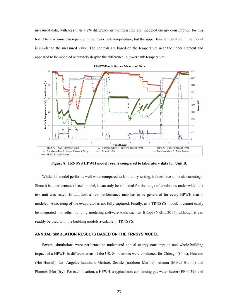
modeled performance for Draw Profile 1 is given in Figure 8. The model results compare favorably to

27

measured data, with less than a 2% difference in the measured and modeled energy consumption for this

test. There is some discrepancy in the lower tank temperature, but the upper tank temperature in the model

is similar to the measured value. The controls are based on the temperature near the upper element and

appeared to be modeled accurately despite the difference in lower tank temperature.

Figure 8: TRNSYS HPWH model results compared to laboratory data for Unit B.

While this model performs well when compared to laboratory testing, it does have some shortcomings.

Since it is a performance-based model, it can only be validated for the range of conditions under which the

test unit was tested. In addition, a new performance map has to be generated for every HPWH that is

modeled. Also, icing of the evaporator is not fully captured. Finally, as a TRNSYS model, it cannot easily

be integrated into other building modeling software tools such as BEopt (NREL 2011), although it can

readily be used with the building models available in TRNSYS.

ANNUAL SIMULATION RESULTS BASED ON THE TRNSYS MODEL

Several simulations were performed to understand annual energy consumption and whole-building

impact of a HPWH in different areas of the US. Simulations were conducted for Chicago (Cold), Houston

(Hot-Humid), Los Angeles (southern Marine), Seattle (northern Marine), Atlanta (Mixed-Humid) and

Phoenix (Hot-Dry). For each location, a HPWH, a typical non-condensing gas water heater (EF=0.59), and

28

an electric storage water heater (EF=0.91) were compared. The gas and electric storage tanks had the same

nominal volume as the modeled HPWH tank. Model parameters for the gas and electric storage water

heaters were based on past work specifically designed to extract the necessary model parameters from the

Energy Factor test results (Burch and Erikson 2004).

Water heaters were evaluated separately for installations in either conditioned or unconditioned space.

Unconditioned space was defined as a basement if a home in that location was likely to have one and a

garage otherwise (ORNL 1988). Homes in Chicago, Seattle, and Atlanta had basements, while the other

homes had a slab foundation. The homes used in the simulations were based on a new construction home

using many of the Building America program guidelines (NREL 2010). However, several simplifications

were made to the homes modeled here, including using a simplified infiltration model (ASHRAE 2009).

The envelope specifications were based upon the ICC 2009 energy conservation code. All of the modeled

homes used an air source heat pump for space heating and cooling with backup electric resistance elements,

and none of the homes had a dehumidifier installed.

The water heater tank losses were assumed to go to either conditioned or unconditioned space,

depending on where the water heater was located. For a gas water heater, 2/3 of the tank losses were

assumed to go to the space while the remaining 1/3 was assumed to go out the flue (US DOE, 2000). All

homes were simulated with a one minute timestep to allow a realistic hot water draw profile to be used. The

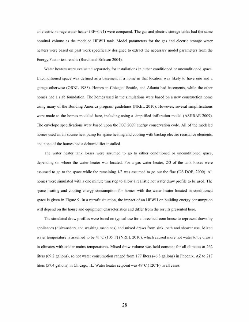
space heating and cooling energy consumption for homes with the water heater located in conditioned

space is given in Figure 9. In a retrofit situation, the impact of an HPWH on building energy consumption

will depend on the house and equipment characteristics and differ from the results presented here.

The simulated draw profiles were based on typical use for a three bedroom house to represent draws by

appliances (dishwashers and washing machines) and mixed draws from sink, bath and shower use. Mixed

water temperature is assumed to be 41°C (105°F) (NREL 2010), which caused more hot water to be drawn

in climates with colder mains temperatures. Mixed draw volume was held constant for all climates at 262

liters (69.2 gallons), so hot water consumption ranged from 177 liters (46.8 gallons) in Phoenix, AZ to 217

liters (57.4 gallons) in Chicago, IL. Water heater setpoint was 49°C (120°F) in all cases.

29

Figure 9: Space heating and cooling source energy consumption for homes modeled in TRNSYS with the water heater in conditioned space

One issue when comparing a HPWH to other water heating technologies is that the HPWH tended to

deliver water at a lower temperature than both the gas and electric water heater. This temperature ‘sag’ was

observed for every water heater, but was more significant for the HPWH. This sag occurred because the

system recovers at a slower rate while using the heat pump. To compensate for this sag during modeling, it

was assumed that any sag for electric water heaters was made up by an 100% efficient electric tankless

water heater placed after the water heater, while the sag for the gas water heater was made up with a gas

tankless water heater with the same efficiency as the combustion efficiency for the gas storage water heater.

SIMULATION RESULTS AND DISCUSSION

The results in this paper are presented in terms of source energy consumption to highlight the

difference between gas and electric water heaters. The source to site ratios used were national averages,

with a ratio of 3.365 applied to the HPWH and electric storage water heater and 1.092 applied to gas water

heater (NREL 2010). Annual source energy consumption of each simulated water heater is reported in

Tables 11 and 12. These results include the space conditioning interactions and energy consumption

differences between water heater technologies and any difference in the energy required to compensate for

30

the sag in the water heater outlet temperature. The change in HVAC equipment loads is different for gas

and electric water heaters due to differences in the tank losses for this equipment, so the HPWH energy

consumption when compared to a gas and electric water heater are presented separately in these tables.

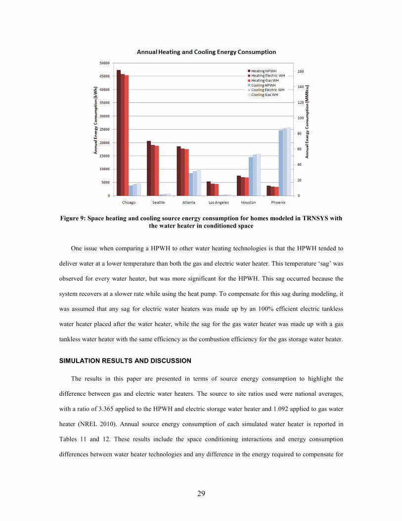
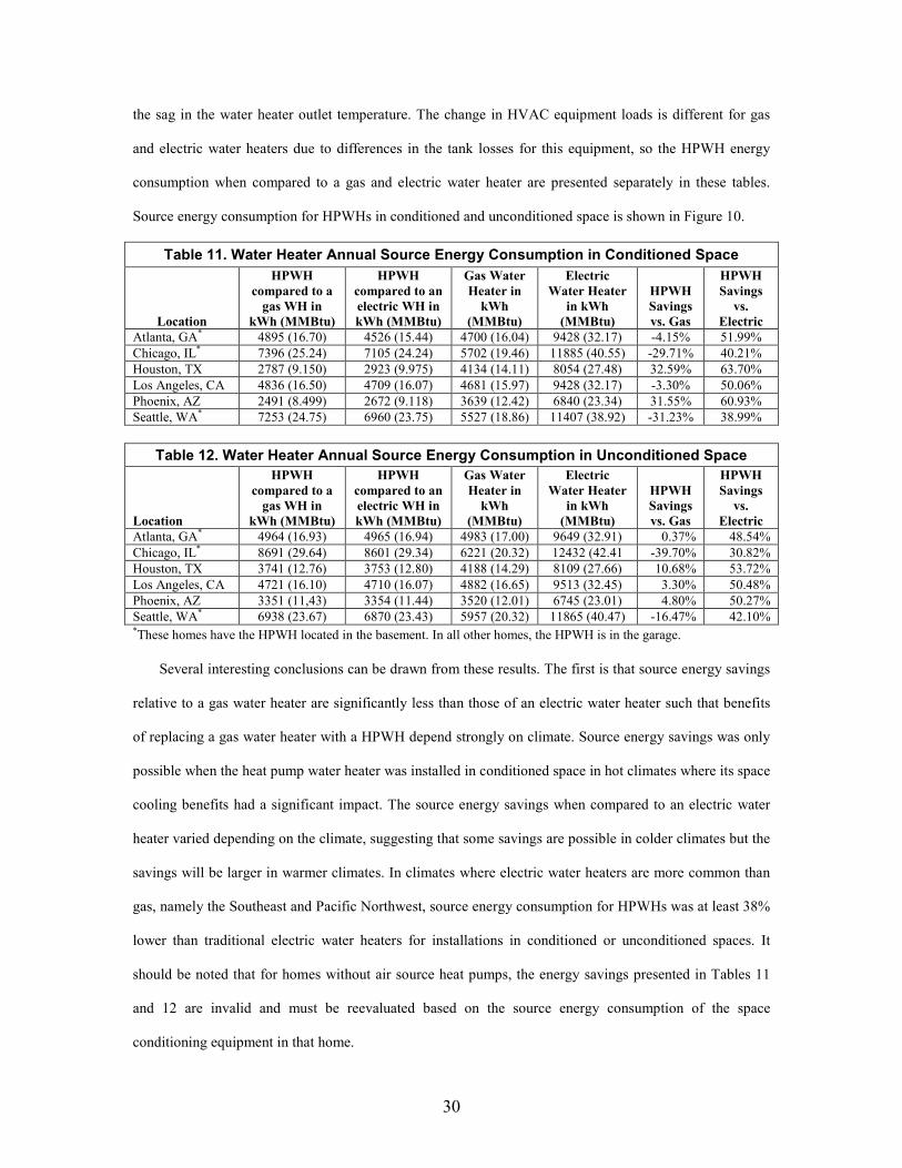
Source energy consumption for HPWHs in conditioned and unconditioned space is shown in Figure 10.

Table 11. Water Heater Annual Source Energy Consumption in Conditioned Space

Location

HPWH compared to a

gas WH in kWh (MMBtu)

HPWH compared to an electric WH in kWh (MMBtu)

Gas Water Heater in

kWh (MMBtu)

Electric Water Heater

in kWh (MMBtu)

HPWH Savings vs. Gas

HPWH Savings

vs. Electric

Atlanta, GA* 4895 (16.70) 4526 (15.44) 4700 (16.04) 9428 (32.17) -4.15% 51.99% Chicago, IL* 7396 (25.24) 7105 (24.24) 5702 (19.46) 11885 (40.55) -29.71% 40.21% Houston, TX 2787 (9.150) 2923 (9.975) 4134 (14.11) 8054 (27.48) 32.59% 63.70% Los Angeles, CA 4836 (16.50) 4709 (16.07) 4681 (15.97) 9428 (32.17) -3.30% 50.06% Phoenix, AZ 2491 (8.499) 2672 (9.118) 3639 (12.42) 6840 (23.34) 31.55% 60.93% Seattle, WA* 7253 (24.75) 6960 (23.75) 5527 (18.86) 11407 (38.92) -31.23% 38.99%

Table 12. Water Heater Annual Source Energy Consumption in Unconditioned Space

Location

HPWH compared to a

gas WH in kWh (MMBtu)

HPWH compared to an electric WH in kWh (MMBtu)

Gas Water Heater in

kWh (MMBtu)

Electric Water Heater

in kWh (MMBtu)

HPWH Savings vs. Gas

HPWH Savings

vs. Electric

Atlanta, GA* 4964 (16.93) 4965 (16.94) 4983 (17.00) 9649 (32.91) 0.37% 48.54% Chicago, IL* 8691 (29.64) 8601 (29.34) 6221 (20.32) 12432 (42.41 -39.70% 30.82% Houston, TX 3741 (12.76) 3753 (12.80) 4188 (14.29) 8109 (27.66) 10.68% 53.72% Los Angeles, CA 4721 (16.10) 4710 (16.07) 4882 (16.65) 9513 (32.45) 3.30% 50.48% Phoenix, AZ 3351 (11,43) 3354 (11.44) 3520 (12.01) 6745 (23.01) 4.80% 50.27% Seattle, WA* 6938 (23.67) 6870 (23.43) 5957 (20.32) 11865 (40.47) -16.47% 42.10% *These homes have the HPWH located in the basement. In all other homes, the HPWH is in the garage.

Several interesting conclusions can be drawn from these results. The first is that source energy savings

relative to a gas water heater are significantly less than those of an electric water heater such that benefits

of replacing a gas water heater with a HPWH depend strongly on climate. Source energy savings was only

possible when the heat pump water heater was installed in conditioned space in hot climates where its space

cooling benefits had a significant impact. The source energy savings when compared to an electric water

heater varied depending on the climate, suggesting that some savings are possible in colder climates but the

savings will be larger in warmer climates. In climates where electric water heaters are more common than

gas, namely the Southeast and Pacific Northwest, source energy consumption for HPWHs was at least 38%

lower than traditional electric water heaters for installations in conditioned or unconditioned spaces. It

should be noted that for homes without air source heat pumps, the energy savings presented in Tables 11

and 12 are invalid and must be reevaluated based on the source energy consumption of the space

conditioning equipment in that home.

31

Figure 10: Annual HPWH net energy consumption. Change in space heating and cooling energy consumptions is based on a comparison to a home with an electric water heater.

One issue that was not fully captured in the modeling is that the “sag” in the outlet temperature in an

actual home is not made up by a tankless water heater. In reality, drops in the outlet temperature could lead

homeowners to either use less hot water, increase the set point temperature of their water heater to increase

comfort, or change the HPWH operating mode, thus increasing the energy used by the HPWH.

Another issue is that performance of the unit when the ambient temperature was out of the operating

range of the heat pump was estimated based on the water heater's performance in electric only mode. It is

possible that the unit behaves differently when in an operating mode that uses the heat pump and the air

temperature is out of range than when it is in electric only mode, but this was not fully explored during

testing. Although these conditions occurred very infrequently during the simulations, the simulation results

did not match up with the measured data as well for this case as for when the unit is using the heat pump.

The next step is to develop and validate an adequate HPWH model in EnergyPlus, to be incorporated

into a whole-house optimization tool such as BEopt. This will be done by applying lessons learned from the

TRNSYS model to modify the EnergyPlus model. It is intended that this updated model will be generic and

represent the family of heat pump water heaters currently available on the market.

32

The annual simulation results outlined in this paper were generated using a model for a new home. An

additional study will need to be performed on existing homes to determine the energy savings for retrofit

applications, where a significant number of HPWHs are expected to be installed.

SUMMARY AND CONCLUSION

The results of the HPWH laboratory performance testing, and the follow-on modeling efforts, confirm

that this technology offers a competitive and energy-efficient alternative to electric resistance water

heating. Data was collected that demonstrates the technology’s capabilities and expands the knowledge of

its performance from a single EF value to COP values across a wide range of operating conditions.

Simulated draw profiles gave insight into how this technology will perform in a real life situation. It

was shown that the size of the storage tank and the unit’s control logic play a significant role in the

performance of a HPWH in high demand situations in terms of both energy efficiency and hot water

delivery. Optimizing the control logic for these first generation units will improve their performance and be

vital to the longevity of this emerging technology. Based on our results, Unit B’s control logic does not

revert back to the heat pump during a heating cycle once the heating elements are enabled, even when

demand is reduced. Also, Unit D’s control logic waits until most of the tank is full of cold water before

turning on the heat pump, a problem that could be fixed by adding a thermistor to the bottom of the tank.

The overall system design is also essential. The appropriate balance between recovery time and

operating range is needed, and some of these units could benefit from improved system designs. For

example, Unit C recovers quickly due to the design of the system, but is limited in operating range because

of it. In addition, Unit C was designed to operate with a fully-mixed tank, which could lead to hot water

delivery issues in high-demand situations. Design changes could significantly improve the performance of

this unit. Another example is Unit B. The heat pump is sized for efficient recovery. However, in high-

demand households, the efficiency of the heat pump would likely go unnoticed because the electric

resistance elements would be needed to meet the hot water demand.

The measured data was used to assess the current HPWH model available in EnergyPlus and an

additional model developed in TRNSYS. Although both codes currently have some limitations, their ability

to model the laboratory data with reasonable accuracy is encouraging. Future efforts to model HPWHs in

33

an accurate, yet comprehensive, manner is essential for representing HPWHs in whole-building

simulations. Modeling a HPWH’s interactions with its immediate surroundings and the other systems

within a house is essential, and will help determine both optimal climatic regions and preferred installation

locations within a specific home. Preliminary annual simulation results show HPWHs are expected to save

a significant amount of energy in most climates for newly constructed homes when compared to electric

resistance water heaters, but are not generally beneficial when compared to gas water heaters.

It is seen that in most climates, installing a HPWH in conditioned space results in a savings in source

energy of over 38% relative to an electric resistance water heater when the impact on the space heating and

cooling loads is considered. Installing a HPWH in unconditioned space results in a reduction in savings in

most climates relative to installing in conditioned space, with the savings ranging between about 30-55%.

When compared to a gas water heater, installing a HPWH in conditioned space results in less than 35%

source energy savings in all climates, with increased energy consumption in cold climates, mixed humid

climates, and the marine climate region. In unconditioned space, the energy savings relative to a gas water

heater are modest, with the most significant savings being slightly over 10%.

In the end, the main advantage of this technology is that it can operate efficiently across a wide range

of conditions, making it a feasible option in many climate zones, in both conditioned and unconditioned

spaces. This makes HPWHs an attractive option for many retrofit applications. The first generation units

included in this report could be improved upon in terms of control logic, system design, and usability, but

in general, the future of heat pump water heaters as an energy saving technology is very promising.

34

REFERENCES American Society of Heating, Refrigerating and Air-Conditioning Engineers, Inc (ASHRAE). 2005.

Methods of Testing for Rating Electrically Driven Unitary Air-Conditioning and Heat Pump Equipment. ANSI/ASHRAE Standard 37-2005.

American Society of Heating, Refrigerating and Air-Conditioning Engineers, Inc (ASHRAE). 2009. ASHRAE Handbook-Fundamentals. ASHRAE Inc.

Ashdown, B.G. 2004. Heat Pump Water Heater Technology: Experiences of Residential Consumers and Utilities. Oak Ridge National Laboratory, Oak Ridge, TN.

Burch, J., and Erickson, P. 2004. Using Ratings Data to Derive Simulation-Model Inputs for Storage Tank Water Heaters. Proc. 29th National Passive Solar Conference.

Calm, J.M. 1984. Heat Pump Water Heaters. Electric Power Research Institute (EPRI), Palo Alto, CA. Consumer Energy Center. 2011. Water Heaters. Retrieved May 16, 2011, from

http://www.consumerenergycenter.org/home/appliances/waterheaters.html Davis, R. 2010. Laboratory Evaluation of Residential Heat Pump Water Heaters. Pacific Gas & Electric

Applied Technology Services. Department of Energy (DOE). 1998. 10 CFR Part 430 Energy Conservation Program for Consumer

Products: test Procedure for Water Heaters, Federal Register Vol. 63, No. 90. Department of Energy (DOE). 2010. Buildings Energy Data Book, http://buildingsdatabook.eren.doe.gov/. D&R International. 2010. Energy Star Water Heater Market Profile. Depart. of Energy, Washington, DC. EnergyPlus. 2010. Version 6.0 Documentation. Energy Star. 2011. 2011 Federal Tax Credits for Consumer Energy Efficiency. Retrieved May13, 2011,

from http://www.energystar.gov/index.cfm?c=tax_credits.tx_index Hashimoto, K. 2006. Technology and Market Development of CO2 Heat Pump Water Heaters (ECO

CUTE) in Japan. Central Research Institute of Electric Power Industry. Nagasaka, Japan. Hendron, R., and Burch, J. 2007. Development of Standardized Domestic Hot Water Event Schedules for

Residential Buildings. Proc. Energy and Sustainability 2007. Hepbasli, Arif., et al. 2009. A Review of Heat Pump Water Heating Systems. Renewable and Sustainable

Energy Reviews 13, pgs. 1211-1229. Klein, S.A., et al. 2010. TRNSYS Users Manual. University of Wisconsin Solar Energy Laboratory,

University of Wisconsin, Madison, WI. Kruis, N. 2010. Reconciling Differences Between Residential DX Cooling Models in DOE-2 and

EnergyPlus. Fourth National Conference of IBPSA-USA. New York, New York. Levins, W.P. 1982. Estimated Seasonal Performance of a Heat Pump Water Heater Including Effects of

Climate and In-House Location. Oak Ridge National Laboratory, Oak Ridge, TN. Maguire, Jeff. 2011. A Parametric Analysis of Residential Water Heaters. Master’s thesis, Department of

Mechanical Engineering, University of Colorado, Boulder, CO. Morrison, G.L. 2003. Seasonal Performance Rating of Heat Pump Water Heaters. School of Mechanical

and Manufacturing Engineering, University of New South Wales, Sydney, Australia. NREL. 2010. Building America House Simulation Protocols. Residential Buildings Research, Golden, CO. NREL. 2011. Building Energy Optimization (BEopt) software. Golden, Colorado.

http://www.nrel.gov/buildings/energy_analysis.html#beopt Oak Ridge National Laboratory (ORNL). 1988. Building Foundation Design Handbook. ORNL, Oak

Ridge, Tennessee. Sparn, B. 2011. Residential Heat Pump Water Heater Evaluation Project. National Renewable Energy

Laboratory, Golden, CO. TESS. 2007. Documentation for Heat Pump Water Heater Type 938. Thermal Energy System Specialists,

Madison, Wisconsin TESS. 2004. Documentation for Stratified Storage Tank Type 534. Thermal Energy System Specialists,

Madison, Wisconsin. US Department of Energy (DOE), 2000. Technical Support Document: Energy Efficiency Standards for

Consumer Products: Residential Water Heaters. US DOE, Washington, DC Zimmerman, K. H. 1986. Heat Pump Water Heater Laboratory Test and Design Model Validation. Oak

Ridge National Laboratory, Oak Ridge, TN.