Hebbian learning and plasticity Experiences change the way we perceive, perform, think and plan. They do so physically by changing the structure of the nervous system, alternating neural circuits that participate in perceiving, performing, thinking and planning. A very simplified view of learning would state that learning modulates (changes) the input-output, or stimulus-action relationship of an organism. Certainly our environment influences how we react to it, and our reactions influence our environment. How learning is achieved in central nervous structures is a major focus of Computational Neuroscience. Learning can easily be observed in behavioral experiments, but there are many examples of changes in neural responses after learning, or after experimental manipulations that change the input-output relationships of a stimulus. Neural firing rates, the temporal precision of their firing, their tuning curves or receptive fields, all of these change with learning and experience.

Experience

OrganismStimulus Response Organism

Experience

OrganismStimulus Response Neuron

At the neural level, many different types of changes can be imagined. For example, we saw that recordings from individual neurons in the hippocampus show that these neurons change their "place field" (i.e. responses to location in space) as the animal investigates the experiment. This change could be due to changes in the way visual stimuli affect these neurons (synaptic), or in the way the neurons respond to the same inputs (intrinsic). A very simple example of learning at the organismal level which has been worked out a the neural level is that of sensitization of the gill withdrawal reflex in Aplysia. In the sea mollusk aplysia, a light touch to the animal's siphon results in gill withdrawal.

This reflex response habituates with repeated stimulation, meaning that the reflex response disappears after repetitive stimulation.

If touching the siphon is accompanied by an electrical stimulation to the animal's tail, then the siphon touch elicits a strong withdrawal response again: The noxious stimulus to the tail sensitizes the gill withdrawal reflex.

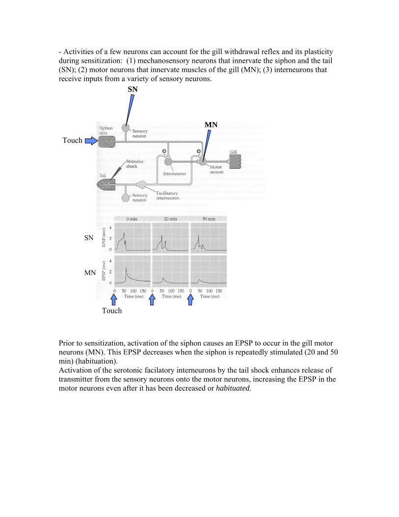
- Activities of a few neurons can account for the gill withdrawal reflex and its plasticity during sensitization: (1) mechanosensory neurons that innervate the siphon and the tail (SN); (2) motor neurons that innervate muscles of the gill (MN); (3) interneurons that receive inputs from a variety of sensory neurons.

SN

MN

SN

MN

Touch

Touch Prior to sensitization, activation of the siphon causes an EPSP to occur in the gill motor neurons (MN). This EPSP decreases when the siphon is repeatedly stimulated (20 and 50 min) (habituation). Activation of the serotonic facilatory interneurons by the tail shock enhances release of transmitter from the sensory neurons onto the motor neurons, increasing the EPSP in the motor neurons even after it has been decreased or habituated.

SN

MN

SN

MN

Touch

Touch

Here, the tailshock has provoked a change in the synaptic interaction between the sensory and motor neuron: transmitter release is increased after the tail is shocked. In modeling terms, this would mean that the synaptic weight has been increased, because the action of a presynaptic neuron (SN) onto a postsynaptic neuron (MN) has been increased. (Reminder: the synaptic weight summarizes the effect a single presynaptic action potential has on the postsynaptic voltage. It includes the amount of transmitter release as well as the maximal conductance change seen at the postsynaptic site and the effect of this conductance change onto the postsynaptic membrane voltage). Using the representation presented above:

Experience Tail shock

OrganismStimulus (Siphon touch)

ResponseGill withdrawl

Organism

ExperienceSerotonine release

OrganismStimulusSN action potential

ResponseMN EPSP

MN

Take another simple example of learning: Pavlov' dog. This "classical" example of classical conditioning was described by the Russian Ivan Pavlov (1849-1936). He trained dogs to associate a tone with a food-reward: (1) the dog initially shows no response to a tone; (2) there is a measurable salivation in response to food; (3) after the tone has been repeatedly presented at the same time than the food, salivation occurs in response to the tone alone in the absence of food. The dog has formed an association between the tone and the food.

Experience Food

OrganismStimulus Tone

ResponseSalivation

Organism

The response function has been changed: previously the stimulus (tone) evoked no response, now the stimulus evokes a response (salivation). This change has occurred because of an experience (food). In the most simple neural network one could imagine, this function can be described as follows:

Sensory neuron (SN)

Food Motor neuron (MN)

Salivation

Auditory sensoryneuron (aSN)

Tone

time

aSN

SN

MN

Food Tone

Before the conditioning, synapses exist between the sensory neurons detecting the presence of food (SN) and the motor neuron driving salivation (MN). No or very weak synapses exist between the sensory neurons detecting the tone (aSN) and the motor neuron (MN). After conditioning, the motor neurons respond to the tone alone, suggesting that synapses have been formed, or strengthened, between the aSN and the MN. In order for this to happen, the tone and the food have to be presented simultaneously. This means that the aSN and the MN have to be active at the same time in order for the synapse to be strengthened. Hebbian learning The idea that connections between neurons that are simultaneously active are strengthened is often referred to as "Hebbian Learning", and a large number of theoretical rules to achieve such learning in neural networks have been described over the years. Historically, ideas about "Hebbian Learning" go far back: in 1890, the Harvard philosopher William James formulated the idea that brain activity is regulated by converging inputs onto a given neuron: (“The amount of activity at any given point in the brain cortex is the sum of the tendencies of all other points to discharge into it, such tendencies being proportionate (1) to the number of times the excitement of each other point may have accompanied that of the point in question; (2) to the intensity of such excitements and (3) to the absence of any rival point functionally disconnected with the first point, into which the discharge might be diverted.”). In 1949, Donald Hebb formulated what became the basis of the idea of "Hebbian Learning" ("When an axon of cell A is near enough to excite a cell B and repeatedly or persistently takes part in firing

it, some growth process or metabolic change takes place in one or both cells such that A’s efficiency, as one of the cells firing B, is increased.”). Today, the expression “Hebbian Learning” refers to a type of plasticity in which change happens as a function of pre and post synaptic activity happening simultaneously at a synapse. Lets think of the two statements above in terms of the formalism we have employed so far: “The amount of activity (action potentials) at any given point (postsynaptic neuron) in the brain cortex is the sum of the tendencies of all other points (presynaptic neurons) to discharge into it, such tendencies being proportionate (1) to the number of times the excitement of each other point (presynaptic action potentials) may have accompanied that of the point in question (synchronous pre- and postsynaptic spiking); (2) to the intensity of such excitements (synaptic strengths/weights) and (3) to the absence of any rival point functionally disconnected with the first point, into which the discharge might be diverted (other postsynaptic neurons, inhibition).”. And : "When an axon of cell A (presynaptic neuron) is near enough to excite a cell B (postsynaptic neuron) and repeatedly or persistently takes part in firing it, some growth process or metabolic change takes place in one or both cells such that A’s efficiency (synaptic strength/weight), as one of the cells firing B, is increased.” Experimentally, a form of hebbian learning has first bee discovered in the hippocampal structure by Bliss and colleagues: when a pyramidal cell in a hippocampal brain slice is depolarized (i.e. active) at the same time that one of its incoming inputs is activated (i.e. a presynaptic neuron fires), the synapse that has been activated becomes strengthened.

5 sec

Recording and injection electrode (intracellular)

Stimulation electrode (extracellular)

100%

pre

axons frompresynapticneurons

post-injection

post

Pairing

2 hours

post-recording

Post-recording

Synapses can also be strengthened when high frequency stimulation is used to activate the presynaptic fibers.

Recording electrode (intracellular)

Stimulation electrode

Baseline

5 sec

100 Hz tetanus

... 2 hours

100%

Tetanus

pre

post

Axons frompresynapticneurons

When the presynaptic fibers are activated at high frequencies (typically 100Hz, often referred to as tetanus), the postsynaptic neuron is still depolarized from the first pulses when subsequent pulses arrive. In the last 20-30 years, a wealth of data has been accumulated on the properties and mechanisms underlying long-term-potentiation as well as long-term-depression (a decrease of synaptic strength). At the same time, neural network modeling and computational neuroscience research has analyzed the theoretical implications for LTP and learning. Evidence for the involvement of LTP in learning. Evidence that long term potentiation (often studied in brain slices) may be involved in learning in the behaving animal comes from a number of observations (by no means a complete list): (1) LTP can be obtained by electrical stimulation in in vivo preparations as well as in behaving animals; (2) animals in which NMDA receptors have been blocked are impaired in certain memory tasks like the radial maze or the water maze; (3) genetically engineered mice which have no NMDA receptors in the hippocampal formation CA1 are impaired on spatial learning tasks AND pyramidal cells in this brain area have less precise spatial receptive fields; (4) in a study using electrical stimulation in the olfactory bulb as cues for olfactory discrimination, an enhancement of the evoked potentials was observed ONLY for stimulations paired with a reward; (5) neuromodulators like acetylcholine, which enhance or enable LTP formation in brain slice experiments impair learning in behavioral situations. Hebbian learning rule The formulation of associative learning that has gathered the most attention for those studying the brain was due to Donald Hebb (see quote above).

This proposition has led to a number of mathematical rules, the simplest of which is: Δwij = μ xi xj where Δwij is the change in the synaptic weight connecting neuron j to neuron i and xi and xj are the activities (firing rates, action potentials) of neurons i and j, and μ is a scaling parameter often called learning rate.

wij

Neuron j Neuron i

xi = F[wij xj] F: linear or non-linear function transforming input into output activity

Δ wij = μ xi xj change in synaptic weight Reminder: wij stands for the synaptic weight between presynaptic neuron j an postsynaptic neuron i. One way to interpret this rule is that each time neurons i and j each fire an action potential, the synaptic weight between them is increased. A second interpretation is that the synaptic weight between them is increased proportionally to the average firing rates of both neurons. A third interpretation is that whenever neuron j fires, the synaptic weight wij is increased by a factor proportional to the activity (voltage) in neuron i: Δwij = μ vi xj In 1973, Bliss and Lomo first published evidence for a biological mechanism leading to associative change in synaptic strength between neurons.. Exercise. Use two McCulloch Pitts neurons. The first one receives external input I. Its output is binary (0 = inactive; 1 =active). It makes an excitatory synapse onto the second neuron. Both neurons have a threshold of 0.5. The synaptic weight is 1.0. Imagine I switches between 1.0 and 0.0 at every time step. Given a learning rate of μ = 0.1, and a Hebbian Rule Δwij = μ xi xj draw the evolution of the synaptic weight during 20 time steps. What happens to the neurons’ activities” Do they change? What is the issue here? This learning rule, as well as the experimental observation underlying it, is associative. This refers to the fact that both the pre- and postsynaptic neuron need to be activated at the same time (reminder: at the same time is a relative statement in biology) for the change in synaptic weight (or efficacy) to work. Because of this property, the Hebbian learning rule can serve to form associations between the activity in the pre- and postsynaptic neurons. The associative nature of long term potentiation (LTP) can be due to two important properties of a synaptic receptor called NMDA receptor. When the neurotransmitter glutamate is released from the presynaptic terminal of many synapses in the brain, it binds to (at least) two kinds of postsynaptic receptors. Binding to the first kind of receptor, called AMPA receptor, leads to rapid increase of current (and depolarization) in the postsynaptic cell. possibly contributing to spiking in this cell.

1) Action potential in the presynaptic terminal leads to release of glutamate. 2) Glutamate binds to AMPA receptors on the postsynaptic membrane. The binding process changes the confirmation of the protein in such a way as to increase its conductance and 3) Na+ ions can now enter the cell. The resulting current depolarizes themembrane of the postsynaptic neuron (positive ionsenter cell -> inside of cell becomes more postive withrespect to outside -> depolarization).

AMPA receptor

The action of glutamate on the second kind of receptor, called NMDA receptor, is more complicated. When the postsynaptic membrane is at potentials close to the resting membrane potential (~ 55-75 mV), the NMDA channel is blocked by magnesium ions (imagine these ions sitting in the receptor and blocking the access for glutamate). This magnesium block is voltage dependent and it is relieved when the postsynaptic neuron is depolarized to near or above firing threshold. Therefore, for current (+ions) to enter the cell through the conductance linked to NMDA receptors, presynaptically released glutamate needs to bind to these receptors, AND the postsynaptic neurons needs to be depolarized in order to unblock the NMDA receptors. As a consequence, both pre (glutamate release) and post (depolarization) neurons need to be active in order for current to pass through NMDA-type conductances.

NMDA receptor when postsynaptic neuron is at rest1) Presynaptic neuron fires an action potentialand releases glutamate. 2) because postsynaptic neuron’s membrane is near resting potential, Mg2+ ions blockthe NMDA receptors. Glutamate cannot bind to NMDA receptors and conductance is not changed -> no depolarization of postsynaptic cell.

NMDA receptor when postsynaptic neuron is depolarized

1) Presynaptic neuron fires anaction potential and releases glutamate. 2) Because postsynaptic membrane is depolarized, Mg2+ ions are expelled from the NMDA channel. 3) Glutamate binds to NMDA receptor, which leads to an increase in conductance in the channel linked to NMDA. 4) Na+ and Ca2+ ions enter the cell and cell depolarizes.

A second important property of the NMDA channels is that part of the current they pass through is carried by calcium ions. A host of experimental results indicate that calcium then leads to a cascade of cellular events which eventually lead to LTP (strengthening of synapses). If we consider that the opening of the conductance leading to the influx of Ca2+ into the cell necessitates both the presynaptic activation (release of glutamate) and

the postsynaptic activation (release of magnesium block), then the NMDA channel provides the substrate to implement the "Hebbian learning rule". The action of the NMDA channel is the basis for the multiplication in the equation governing the changes in synaptic strength: potentiation of synaptic strength occurs only if the presynaptic activity xj > 0 (glutamate release) and if the postsynaptic activity vi > 0 (depolarization, or xi > 0 action potential). In order to ensure that only depolarization is taken into account, the equation is rewritten as: Δwij = μ F[vi] xj, where F is a linear threshold function. Of course, when the Δwij = μ xi xj form of the equation is used firing rates can only be positive. So lets apply this learning rule to our example based on Pavlov’s experiments with dogs:

Sensory neuron (SN)

Food Motor neuron (MN)

Salivation

Auditory sensoryneuron (aSN)

Tone

time

aSN

SN

MN

FoodTone

FoodTone

FoodTone Tone

...

Lets assume that the synapse between the aSN and the MN is weak at the beginning, whereas the synapse between the SN and MN is strong enough to fire the MN. We have: Output (SN) = 1.0 when there is food visible Output (aSN) = 1.0 when there is a tone audible Input (MN) = WMN, SN * Output (SN) + WMN, aSN * Output (aSN) Output (MN) = 1.0 if Input (MN) >= ΘMN Output (MN) = 0.0 if Input (MN) < ΘMN In order to have the MN fire in response to food irrespectively of the tone, WMN, SN * Output (SN) >= ΘMN and since Output (SN) = 1 when there is food, we know that WMN,

SN needs to be at least 1.

In order to not have the MN fire in response to the tone (initial state) irrespectively of the food, WMN, aSN * Output (aSN) < ΘMN and since Output (aSN) = 1 when there is a tone, we know that WMN, SN needs to be smaller than 1. So, lets start with WMN, SN = 0.1 and WMN, SN = 1.0. and lets assume for now that only the synapse between the aSN and the MN changes its synaptic strength.

SN

aSN

MN

WMN, SN

WMN, aSN

Food

Tone

SN

aSN

MN

WMN, SN

WMN, aSN

Food

Tone

During every time step that both aSN and MN are firing, WMN, SN is incremented by 0.1. Going back to our simple block diagram:

aSN MNWMN,aSN

Hebbian learning rule

In this case, the modulation of synaptic strength necessitates that MN is activated via a different pathway (SN, food) in order to strengthen WMN, aSN. One obvious problem with this learning rule can be seen immediately: if nothing else is added, WMN, SN will grow forever! In the case of non-linear neurons, this does not have to be a problem because the activity is bounded, but it is certainly not a realistic assumption. In many cases, the learning rule includes an upper values which the synaptic weights cannot exceed. A second observation is that under this learning rule, synaptic strength can only increase and not decrease. Here, biology seems to come to the rescue with a phenomenon called LTD or long term depression. By stimulating the presynaptic neurons at a weaker intensity, synapses can be made to decrease. Subsequent hypotheses have led to the assumption that low levels of calcium entering the postsynaptic cell lead to depression whereas high levels lead to potentiation. The learning rule can be rewritten as:

Δwij = μ xj (F[vi] - φ), where F is a linear threshold function ensuring that only positive (depolarizing) values of v are taken into account and φ is the voltage (postsynaptic) above which LTP will occur. Lets revisit our neurons for a moment. In general, we consider that neurons receive weighted inputs from other neurons. These inputs are somehow transformed into an "output activity" value x(t), which can represent different aspects of neuronal activity. 1) The most straightforward case is that x(t) represents that neuron’s action potential. In that case, x(t) can be either 1 (there is an action potential), or 0 (there is no action potential) at this moment in time. Here, x(t) is a discrete variable (can only take on two discrete values). 2) In many cases, x(t0) represents some kind of "average" firing rate, or instantaneous firing rate, or firing probability. x(t) is then a continuous variable representing how much a neuron is firing at a given time. For example, x(t) could vary between 0 and 1, representing the probability that the neuron emits a spike at any given time, or x(t) could vary between 0 and 100, representing the neurons average , or sometimes instantaneous firing rate (in Hz).

time

timeFiring rate (Hz)Firing probability

Action potentials

Both of these representations of a neurons "activity" can be used to in Hebbian learning rules. In case 1, timing will become very important, because the learning rule would be formulated as : Δwij = μ xi xj at any given time t, so only if both neurons are active (x = 1) at exactly the same time step will the weight increase. In case 2, both xi and xj are continuous variables and thus timing becomes of less importance. Exercise ! About LTP with and without threshold! Lets calculate an example. The hebbian learning rule and associators Previously, we talked about a common way to calculate changes in connection strengths in a neural network, the so called “Hebbian Learning Rule”, in which a change in the strength of a connection is a function of the pre – and postsynaptic neural activities. If xj is the output of the presynaptic neuron, xi the output of the postsynaptic neuron, and wij the strength of the connection between them, and γ learning rate, the one form of a learning rule would be: ΔWij (t) = γ∗xj*xi

A more general form of a hebbian learning rule would be: ΔWij (t) = F(xj, xi, γ, t, θ) in which time and learning thresholds can be taken into account. Time We often say that the connection strength, or synaptic weight, of a synapse increases when the pre- and postsynaptic neurons are active “simultaneously”. Simultaneous is very relative depending on the system under consideration! For example, when synaptic plasticity is induced in a brain slice preparation, simultaneous can be as short as several ms. However, when an animal learns an association between a food taste and sickness, simultaneous can be as long as several hours! Exercise. Brainstorm some meaning of simultaneous that you can think of which are relevant to learning and memory. Example we talked about in class Classical conditioning can be modeled with a hebbian synapse. Consider an unconditioned stimulus (an air puff), an unconditioned response (eye blink), a conditioned stimulus (a tone) and a conditioned response (eye blink). Under normal conditions, an animal responds to an air puff with an eye blink. It does not respond to a tone with an eye blink. If the tone is paired with the air puff several times, then the animal acquires an association between the airpuff and the tone, and will now respond to the tone alone with an eye blink. Consider a “black box” neural approach where one neuron receives input from the airpuff and from the tone. The neurons output represents the eye blink. The neuron is wired in such a way that at first, the airpuff but not the tone activates the neuron and produces an output. If we apply the airpuff input and the tone input together several times, then the neuron is active while the tone-input is active, and a hebbian learning rule will reinforce the strength of the connection between the tone and the neuron. This will lead to the fact that after a few trials, the tone alone will be able to activate the neuron. Neurons of this type can be recorded in the amygdala.

Σtone

airpuff

eyeblink Σtone

airpuff

eyeblink

timeairpuff

tone

weight

airpuffeyeblink

weight

Exercise: Generalization refers to a phenomenon in which animals respond to stimuli other than the one they have been conditioned to after conditioning. For example, if a dog is conditioned to salivate in response to a 440 Hz tone, it may later also salivate to tones with close by frequencies such as 400, 420, 460 or 480 Hz. The more different the stimulus is from the conditioned one, the less the dog would “generalize” to it. In this exercise, explain how the combination of hebbian learning rule and broad sensory tuning curves could explain behavioral generalization. Tuning curves change with experience: application of the Hebbian Learning Rule So far our discussions of tuning curves have revolved around the idea that these are relatively stable and “innate”. In real life, tuning curves change commonly as a function of experience, behavioral demands on the animal and physiological state. In this section we will examine how interactions between neurons paired with a Hebbian Learning Rule can lead to changing tuning curves. Readings: Knudsen EI. Instructed learning in the auditory localization pathway of the barn owl. Nature 417: 322-328, 2002 and references therein. Feldman, DE and Brecht, M. Map plasticity in somatosensory cortex. Science. 2005 Nov 4;310(5749):810-5. and references therein.

Application of the hebbian learning rule: the linear associator Take a network of neurons which are organized in two distinct layers (called f and g). Neurons in layer f project to neurons in layer g but not vice versa (this would be called a "feedforward organization"). Each neuron in layers g and f is a linear unit, its output x is the sum of its inputs i (hence the name linear associator). xi = Ii where xi is the neuron's output, Ii is the total input to that neuron. Remember that this means that a neuron's output can take on arbitrary values which represent mean activation values or firing rates (but not individual action potentials). The strength of the connection form presynaptic neuron fj to postsynpatic neuron gi is given by wij. Reminder: wij connection from neuron j to neuron i. The activation of each neuron in the layer g is given by is sum of weighted inputs from the neurons in layer f. xi = Σwij xj where xj are the outputs from the presynaptic neurons in layer f and wij are the corresponding connection strength or synaptic weights. The strength of each connection is calculated from the product of the pre- and postsynaptic activities scaled by a “learning rate” γ (which determines how fast connection weights change). Δwij = γ * gi * fj. If you don't want to write down the individual equations for each neuron, you can write a vector notation: Vectors are lists of numbers:

⎥⎥⎥⎥⎥⎥⎥⎥

⎦

⎤

⎢⎢⎢⎢⎢⎢⎢⎢

⎣

⎡

=

fn..fj

2f1f

f and

⎥⎥⎥⎥⎥⎥⎥⎥

⎦

⎤

⎢⎢⎢⎢⎢⎢⎢⎢

⎣

⎡

=

gn..gi

2g1g

g

In order to multiply these two vectors, we have to "transpose" one of them:

gT = [g1, g2, .. gi, .. gn], then : [ ]fn...fi,..2f,1f

gn..gj

2g1g

⎥⎥⎥⎥⎥⎥

⎦

⎤

⎢⎢⎢⎢⎢⎢

⎣

⎡

=γ= f Tg w this is called the "outer

product" (as opposed to the "inner product" or "dot product, scalar product" (a = gTf) and

⎥⎥⎥⎥

⎦

⎤

⎢⎢⎢⎢

⎣

⎡

===

====

=

fngn wnn... gnf2 w2n1gnf1wn

1f2g21wg1fn w1n... g1f2 w121f1g11w

w

is the resulting matrix of synaptic weights.

layer f layer g

f1

f2

fj

fn

g1

g2

gi

gn

weight matrix w

w11

w12

w1n

g1 = x(f1) w11 + x(f2) w12 ... x(fj) w1j ... + x(fn) w1n gi = x(f1) wi1 + x(f2) wi2 ... x(fj) wij ... + x(fn) winetc ..

The linear associator stores associations between a pattern of neural activations in the input layer f and a pattern of activations in the output layer g. Once the associations have been stored in the connection weights between layer f and layer g, the pattern in layer g can be “recalled” by presentation of the input pattern in layer f. Lets look at a familiar example, that of your grandmother. Lets assume that when you were a child, your grandmother would often bake a specific type of cookie, and that you learned to associate the smell of those cookies baking with the sound of your grandmother's voice. So, we have one layer of neurons receiving inputs from your auditory system (layer g), and one layer of neurons receiving input from your olfactory system (layer f). Neurons in layer g have receptive fields that are arranged such that some of them will respond more or less every time you smell the specific cookies, and neurons in layer g have receptive fields that can respond to your grandmothers voice.

Olfactory system Auditory system

Grandmother baking cookies and talking

At first., smelling cookies will activate some neurons in layer g, but will have no or little effect on the neurons in layer f because the synaptic weights between neurons in layer g and f are weak or zero. When you experience your grandmother's voice and the cookie smell at the same time, the synapses or connections between layer f (responding to olfactory stimuli) and layer g (responding to auditory stimuli) are changed via the hebbian learning rule. Δwij = γ * gi * fj. The learning rule will affect only connections between neurons that are both active. Lets assume neurons depicted in black and gray are activated above threshold, and neurons depicted in white are inactive. The following synapses will undergo "learning":

Olfactory system Auditory system

Grandmother baking cookies and talking

Assume that the outputs x of active neurons are 1, the learning rate is 1.0, and the initial synaptic weights are 0.0. Then, for all synapses connecting to active neurons,

Δwij = γ * gi * fj. = 1.0*1.0*1.0 = 1.0, and the resulting synaptic weights are 1.0. Subsequently, if you smell the specific cookies your grandmother used to bake, the smell will "evoke" the sound of her voice by reactivating the neurons that were initially responding to the voice. The system has formed an "association" between the smell and the voice.

Olfactory system Auditory system

Cookies

x(gi) = Σ wij * x(fj)

If you smelled a very different smell from the one you learned to associate with your grandmother's cookies, the voice would not be evoked.

Olfactory system Auditory system

Bread

x(gi) = Σ wij * x(fj)

But if you smelled a smell that was only slightly different (or overlapping) with the cookie smell, the voice might be evoked to a lesser degree!

Olfactory system Auditory system

Cookies

x(gi) = Σ wij * x(fj) If you had an aunt that was cooking delicious stews and talking while she was cooking, you might form a second association between a smell and a voice!

Olfactory system Auditory system

Aunt cooking stew and talking

But if your aunt was baking cookies very similar to those your grandmother was baking and your brain was really functioning as a linear associator, you may become confused as to whose voice is whose!

Olfactory system Auditory system

Aunt baking cookies and talking

Grandmother’s voice recalled!

Examples will be calculated in class! Auto-associative memory Next, we will further explore associative memory circuits and look at a different type of associative memory circuits called auto-associative memory. In an auto associative memory, different parts of a same pattern are associated with each other (as opposed to an associative memory network, in which two patterns are associated with each other). Imagine that you smell a certain smell which activates a number of neurons in your olfactory cortex to various degrees: input from olfactory bulb

feeback interactions(association fibersintrinsic cnnection)

output

Now imagine that excitatory synapses exist between all pairs of neurons in the cortical network (fully connected). If all of these synapses obey a hebbian learning rule, than the weights of all synapses between neurons that are simultaneously active will be increased.

input from olfactory bulb

feeback interactions(association fibersintrinsic cnnection)

output

Now if you reactivate the pattern only partially (you smell a similar or a weaker smell), because of the existing strong synapses, the original pattern will be reactivated. An illustrative example is that of a face:

Once the pattern has been stored by creating strong excitatory connections between all pixels (neurons) that are active (black), a partial presentation of the pattern will lead the recall of the initial pattern. A particularly important class of neural networks which fulfill associative memory functions are so called "Hopfield networks", which have a recurrent structure and the development of which is inspired by statistical physics. They share the following features:

• Nonlinear computing units (or neurons) • Symmetric synaptic connections (wij = wji) • No connections of a neuron on itself (wii = 0) • Abundant use of feedback (usually, all neurons are connected to all others)

(Feedback means that a neurons sends a synapse to a neuron it also receives a signal from, so that there is a closed loop). Most often (for a network with N units, where xi is the activation value of unit i, wij the weight of the connection between unit j and unit i, and E an energy function):

state] previous itsin remains junit 0 [if 0 if 1-0 if 1

{ and * vvvxxwv i

N

1j i

iijiji =

<>+

== ∑=

ji if 0 j i if *N1 wxxw ijjiij ==≠=

∑∑= =

−=N

1i

N

1jjiij **

21E vvw

Among others, the Hopfield network is a recurrent network that embodies the storing of information in a dynamically stable configuration. Hopfields idea was that of locating each pattern that was to be stored at the bottom of the valley of an energy landscape, and then permitting a dynamical procedure to minimize the energy of the network in such a way that the valley becomes a basin of attraction. Imagine that you place a marble on the wall of a container. It may role a round for a while (trajectory), but no matter where you throw it in (initial condition), will always end up on the bottom (minimum).

Initial condition

Trajectory

Minimum Similarly, if you have a pendulum, you can start it from any given location, it will always eventually end up in the same location no matter where you start it from. What changes from trial to trial is how long it takes to settle down. In a neural network with binary threshold neurons (or McCulloch Pitts neurons) and symmetric weights, one can calculate the synaptic weights in such a way as to create a "minimum" into which the networks activity will settle. In the example above, the initial position, trajectories and the minimum are given by locations in space; in a neural network these would be characterized by the "activation pattern" or the vector representing the activation pattern of the neurons in the network. In physical examples, the minimum is defined by the physical dimensions as well as by the law of gravity (the marble will roll to the lowest possible location, the pendulum will stop at the location in which lateral forces on it are zero); in a neural network the minimum will be defined by the synaptic weights between the neurons.

Minimum at (0,0,0)

The idea is that in a network of binary threshold units (or McCulloch Pitts units) with symmetric weights (i.e. the weight of the connection from unit i to unit j is the same than that from unit j to unit i), there is a certain pattern of activation of these units that is very stable. For example, if all connection weights were to be +1, then the pattern for which all units have the value +1 is very stable. Once the units all have acquired that value, nothing will change anymore!

N1 N2

w12 w21

v1, v2, v3: inputs to neuron 1, 2x1, x2, x3: outputs of neuron 1,2w12, w21 etc: connection strength

N3

w13

w31w32

w23

w12=w13=w21=w23=w31=w32=1.0 A. t=0 x1=x2=x3=1 initial condition t=1 v1=w12*x2+w13*x3 = 1; x1=1 v2=w21*x1+w23*x3 = 1; x2=1 v3=w31*x1+w32*x2 = 1; x3=1 This will never change, it’s a "stable state" B. t=0 x1=x2=1; x3=-1 initial condition t=1 v1=w12*x2+w13*x3 = 0; x1=1 (stays as is) v2=w21*x1+w23*x3 = 0; x2=1 (stays as is) v3=w31*x1+w32*x2 = 2; x3=1 This will never change, network reached a stable state!

Each particular pattern is called a “state” of the network, and the space of all possible states is called the state space (sometimes also phase space). For example, the state space of a two-neuron network comprises four different states: (-1,-1);(-1,1);(1,-1); and (1,1). For each distribution of connection weights in such a network, there exist a number of stable states, which are also referred to as attractors. In the example above, there are several stable states which coexist with the same connection weights. t=0 x1=-1=x2=-1; x3=1 initial condition t=1 v1=w12*x2+w13*x3 = 0; x1=-1 (stays as is) v2=w21*x1+w23*x3 = 0; x2=-1 (stays as is) v3=w31*x1+w32*x2 = -2; x3=-1 t=2 v1=w12*x2+w13*x3 = -2; x1=-1 v2=w21*x1+w23*x3 = -2; x2=-1 v3=w31*x1+w32*x2 = -2; x3=-1 As one can see, there are at least 2 stable states in this particular network, each with a given "basin of attraction". Initial conditions with two neurons active, one inactive, will go to (1,1,1) and initial conditions with two neurons inactive and one active will go to (-1,-1,-1). An attractor is a point in the state pace to which the activation values of the units want to go, i.e. the attractor has a basin of attraction around it. This means that if for example the point (1,-1) in a two-dimensional space is a stable point, then if we perturb the network (perturb means to add noise, or change a value), in such a way for example that we give the units the values (1.2,-0.8), then the attractor “attracts” those values back, and because of the dynamics of the network the values will become (1,-1) again. Each trajectory terminates at a stable point.

E(1,1,1) = -3

E(-1,-1,-1) = -3

E(-1,1,-1) = 1

E(1,-1,1) = 1

E(-1,1,1)=1

(-1,-1,1)

E(1,-1,-1) = 1

(1,1,,-1)

The stable states or attractors correspond to valleys of the energy function (the energy function is given by the connection matrix, and has a given value for each pattern of unit activations). The stable states or attractors correspond to valleys of the energy function (the energy function is given by the connection matrix, and has a given value for each pattern of unit activations). In the example above, the energy function

∑∑= =

−=N

1i

N

1jjiij **

21E xxw (more or less equivalent to ∑∑

= =

−=N

1i

N

1jjiij **

21E vvw ) corresponds to:

E = -1/2 * (w12*v1*v2+w13*v1*v3+w21*v2*v1+w23*v2*v3+w31*v3*v1+w32*v3*v2) if at t=0 x1=-1=x2=-1; x3=1 then E(t=0) = -1 and at t=1 x1=x2=x3=x4 = -1 then E(t=1) = -3 which is < E(t=0). Similarly, if at t=0 x1=1=x2=-1; x3=1 then E(t=0) = 1 and at t=1 v1=w12*x2+w13*x3 = 2; x1=1 v2=w21*x1+w23*x3 = 2; x2=1 v3=w31*x1+w32*x2 = 0; x3=1 E(t=1) = -0.5*3 = -1.5 < E(t=0) Spurious states or spurious attractors represent stable states of the network that are different from the memories of the network which served to calculate the connection matrix. They arise mainly for two reasons: (1) the energy function is symmetric, such that its values remain unchanged when all the units take on the opposite values of the stored memory (all +1’s are replaced by –1s). As a consequence, if the memory (-1,1,-1) is a stable state, then it’s opposite, (1,-1,1) is also a stable state; (2) There is an attractor for every mixture of stored patterns. Does it work well? Not very well. Not many patterns can be stored, and those should really be orthogonal to be stored perfectly. Is it "realistic"? Not really. First, it necessitates neurons that make both inhibitory and excitatory connections and second it needs symmetric weights. Can one use it as a model for more realistic associative memory circuits? Certainly! Many brain circuits provide the essential ingredients: extensive feedback connections between excitatory neurons as well as a hebbian-like learning rule (LTP).

Can associative memory networks function in brains? In the associative networks we have talked about so far, the patterns of activity to be stored are “clamped” or fixed during the calculation of the necessary synaptic weight changes. Typically, a “learn” phase is distinguished from a “recall” phase. During the learn phase, interactions between the neurons are halted artificially, and during the recall phase, synaptic plasticity is turned off.

Input

Output

Input

Output

Haberly, L.B. Chem. Senses, 10: 219-38 (1985)Haberly & Bower, TINS, 12: 258-64, (1989)

Piriform cortex =? associative memory network

Ia

Ib

II

III

Afferent Input from OB mitral cells (LOT)

AssociationFibers

Ia

Ib

II

III

Afferent Input from OB mitral cells (LOT)

AssociationFibers

to OB, EC, HC ...

Remember that a three layered cortex like the olfactory cortex or the hippocampus has a very similar structure to associative memory circuits proposed by Marr and others. The main features are an afferent input imposing information from outside onto the pyramidal cells within the network, as well as a dense system of intrinsic interactions between pyramidal cell in the network (all-to-all in a neural network, and highly distributed in a cortex).

Associative memory function

Learning

Synapses are strengthened according to some “Hebbian” learning rule

Output Output

Recall

Incomplete input pattern is reconstructed

During learning, an afferent input pattern is mediated to the neurons in the network, and intrinsic synapses are changed according to some hebbian learning rule. A number of learning rules can be employed here, including the Hebbian learning rule we talked about. During recall, an incomplete or distorted version of the input is presented to the network via the afferent fibers and the previously stored memory is recalled or reconstructed thanks to the intrinsic synapses which are specific to previously stored memories. Learning: In these artificial networks, the weight matrix is calculated mathematically, as we have done in the lectures. Often, if more than one pattern needs to be stored, all weight matrices are calculated separately and then added together. This process is of course not terribly realistic. A more realistic approach would be to impose an afferent pattern for a certain amount of time and then have a local hebbian learning rule change the synaptic weights over time. Obviously, in that case, the new synaptic weights would change the pattern of activity as they are updated. In the artifical stituation, all communication between neurons is supposed to be halted when the weights are calculated. Recall: In artifical neural networks, recall is strictly separated from learning. That means that patterns are imposed and at that time, all activity and communication between neurons is halted. After the learning process, the weights are considered frozen, and a pattern is imposed to be "recalled". At this time, learning has been switched off and weights do not change anymore. If a more realistic situation would be considered, then synaptic interactions between neurons would be functioning while synaptic weight changes are calculated; similarly, during recall synaptic weights could still change. There is really no realistic way to think about learning and recall to be separated as cleanly as in our simulations. In a realistic

simulation, all previously stored patterns would interfere with a novel pattern to be stored!

"Clamping" of neural activity during the calculation of synaptic weights is a major component of the theoretical associative memory device

Learning Pattern A

Learning Pattern B

Afferent Input

Neural activities are "clamped" (they don't change)

In theoretical network, neural activity is clampedas if synaptic interaction did not exist. Previously strengthened weights do not affect new weight calculation

In biological network, neural activity is not clampedand previously strengthened weights do affect new weight calculation

Imagine the above small network with 3 neurons. Each neuron can receive afferent input from outside the network as well as intrinsic input from other neurons in the network. During learning, a pattern of activity is typically imposed onto the network via the afferent input. In a more realistic network, already existing synaptic interactions between neurons will change the activity pattern that has been imposed onto the network via afferent input. This can lead to problem with storage of patterns, as can easily be seen. Imagine that you first want to store a pattern A which activates two neurons via afferent input.

Learning Pattern A

After calculating the weight changes for these neurons, you would like to also store a second pattern, which has some common elements with the first one you stored.

Neural activity clamped during learning

Learning Overlapping Pattern B

If synaptic interactions are turned off during the determination of the new synaptic weights, this second pattern can be stored without interference from the previous one. Learning Overlapping Pattern B

Neural activity not clamped during learning

If synaptic interactions are not clamped, the previously strengthened synaptic weights can activate neurons that do not participate in the pattern imposed by afferent input. As a consequence, additional synapses will be strengthened and the overlap between the patterns will be enhanced.

If either one of the two patterns is reapplied by the afferent input, both patterns will be recalled. Even if only the neuron that belonged only to pattern A is reactivated, both patterns A and B can be recalled. Years ago, Mike Hasselmo has proposed a possible solution for this problem which allows to implement associative memory networks in more realistic simulations of brain structures. He proposed that if the neuromodulator acetylcholine was present during the learning phase but not during the recall phase, previously learned synaptic interactions would interfere less with the learning of new synaptic weights. These ideas were firmly based on experimental data showing that in the presence of acetylcholine, the intrinsic synaptic interaction in several brain structures are suppressed whereas the afferent inputs are not affected. In addition, LTP is increased in the presence of acetylcholine and spike adaptation is decreased, effectively making neurons more active.

The data underlying these ideas have been obtained in brain slice preparations of the olfactory cortex and the hippocampus. As discussed before, cortical structures are clearly layered in such a way that afferent inputs, intrinsic interactions and cell body layers are segregated from each other when a slice is cut in the plane which is perpendicular to these layers. Under a microscope, these layers can be easily distinguished and electrodes can be placed under visual guidance.

Ia

Ib

II

III

Afferent Input from OB mitral cells (LOT)

AssociationFibers

Ia

Ib

II

III

Afferent Input from OB mitral cells (LOT)

AssociationFibers

When brain slices of the olfactory cortex or hippocampus layer CA3 are cut, the layers containing the afferent inputs (from the olfactory bulb or from the entorhinal cortex), the intrinsic or association fibers (from other pyramidal cells in the same network) and the cell bodies can be clearly distinguished under a microscope. Stimulation electrodes can be placed in such a way as to stimulate either the afferent input fibers or the association fibers, and recording electrodes can be placed in such a manner as to record the evoked synaptic potentials either extra- or intracellularly. Remember that during electric stimulation, a short pulse of current is delivered close to a bundle of axons, triggering action potentials in many of these axons. The synaptic potentials recorded next to (or in ) the postsynaptic cell correspond to activation of large numbers of synapses by fibers of the same "functional" origin. The effects of neuromodulators can be recorded by adding these to the brain slice. When either the afferent or the intrinsic inputs to pyramidal cells in the olfactory cortex are stimulated electrically, population EPSPs (excitatory postsynaptic potentials) can be recorded and their amplitude can be measured (by either measuring the baseline-to-peak amplitude or by measuring the slope).

Ia

Ib

II

III

Afferent Input from OB mitral cells (LOT)

AssociationFibers

Ia

Ib

II

III

Afferent Input from OB mitral cells (LOT)

AssociationFibers

Stimulate

Stimulate

Record

RecordLayer 1a: afferent

Layer 1b: intrinsic When the cholinergic agonist carbachol is added to the slice, the same electrical stimulation of the intrinsic fibers produces a much smaller (suppressed) EPSP. Remember, an agonist is a chemical substances which can bind to a receptor and have the same, or very similar effects on the neural and synaptic properties than the neurotransmitter or neuromodulator that exists in the brain would have. The suppression obtained under carbachol is specific to the intrinsic fiber stimulation and does not happen when afferent fibers are stimulated.

Ia

Ib

II

III

Afferent Input from OB mitral cells (LOT)

AssociationFibers

Ia

Ib

II

III

Afferent Input from OB mitral cells (LOT)

AssociationFibers

Stimulate

Stimulate

Record

RecordLayer 1a: afferent

Layer 1b: intrinsic

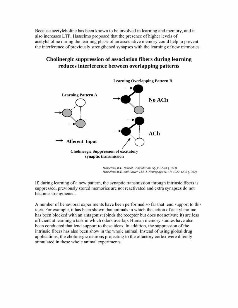
Because acetylcholine has been known to be involved in learning and memory, and it also increases LTP, Hasselmo proposed that the presence of higher levels of acetylcholine during the learning phase of an associative memory could help to prevent the interference of previously strengthened synapses with the learning of new memories.

Cholinergic suppression of association fibers during learning reduces interference between overlapping patterns

Learning Pattern A

Learning Overlapping Pattern B

Cholinergic Suppression of excitatory synaptic transmission

Afferent Input

No ACh

ACh

Hasselmo M.E. Neural Computation. 5(1): 32-44 (1993). Hasselmo M.E. and Bower J.M. J. Neurophysiol. 67: 1222-1238 (1992).

If, during learning of a new pattern, the synaptic transmission through intrinsic fibers is suppressed, previously stored memories are not reactivated and extra synapses do not become strengthened. A number of behavioral experiments have been performed so far that lend support to this idea. For example, it has been shown that animals in which the action of acetylcholine has been blocked with an antagonist (binds the receptor but does not activate it) are less efficient at learning a task in which odors overlap. Human memory studies have also been conducted that lend support to these ideas. In addition, the suppression of the intrinsic fibers has also been show in the whole animal. Instead of using global drug applications, the cholinergic neurons projecting to the olfactory cortex were directly stimulated in these whole animal experiments.

Beyond Vanilla LTP: Spike Timing Dependent Plasticity Experimental data on the induction f LTP and LTD Previously, the induction of LTP and LTD has been thought to depend on the rate of stimulation, number of afferents stimulated and the degree of depolarization obtained in the postsynaptic neuron. For example, in many preparations, electrical stimulation of the presynaptic axons at 100 Hz induces LTP (an increase of synaptic strength on an excitatory synapses) and stimulation at 20 Hz induces LTD (a decrease of synaptic strength of an excitatory synapses). This is thought to be due to the fact that high levels of calcium enter the cell after high frequency stimulation and that low levels of calcium enter the cell after low frequency stimulation. At very low frequencies, neither LTP or LTD are induced.

Recording electrode (intracellular)

Stimulation electrodeRecording electrode (extracellular)

Baseline

5 sec

100 Hz tetanus

... 2 hours

100%

Tetanus

Recording electrode (intracellular)

Recording electrode (extracellular)

Baseline

5 sec

20 Hz

... 2 hours

100%

20 Hz Many formal descriptions of LTP translate these data into simple equations of the form: Δwij = μ * xj * (vi-φ), where xj is the output (action potentials) of the presynaptic neuron j and vi is the membrane potential of the postsynaptic neuron and wij is the synaptic

strength (weight, efficacy) of the synapses from neuron j to neuron i. One can see that if the presynaptic neuron were to fire at 100 Hz, the postsynaptic depolarization would rapidly exceed the threshold for LTP induction (f); however, if the presynaptic neuron were to fire at 20 Hz, the postsynaptic depolarization would stay below the threshold p and the synaptic weight would be decreased. At very low presynaptic firing rates, the postsynaptic depolarization would always return to rest before the occurrence of the next postsynaptic action potential and no changes in synaptic weight would occur.

vi

xj

time

time100 Hz

vi

xj

time

time20 Hz

vi

xj

time

time10 Hz In real life, neurons rarely fire at 100 Hz. One should rather imagine that any individual neuron is receiving inputs from many presynaptic neurons at the same time. In contrast to many previous studies, more recent studies find that the strengthening and weakening of synapses depends on the precise temporal relationship between the presynaptic and the postsynaptic action potentials.

Pre Post

Two pyramidal neurons in a cortical brain slice preparation are simultaneously impaled with intracellular electrodes. Both neurons can have current injected individuallyin such a way as to trigger an action potential. Pre. Im: presynaptic current injection; Pre. APs: presynaptic action potential; Post. Im: presynaptic current injection; Post. APs: presynaptic action potential;

When both neurons are activated to fire at approximately 20 Hz, and the postsynaptic neuron fires 5ms after the presynaptic neuron (is phase locked), then an increase of the synaptic strength between the pre- and postsynaptic neurons can be observed.

Pre Post

pre and post AP's separated by 5 ms

pre

post

20 Hz 20 Hz

4 seconds

10x

Paired

pre-onlypost-only

Markram et al. Regulation of synaptic efficacy by coincidence of postsynaptic APs and EPSPs.Science. 1997 Jan 10;275(5297):213-5.

The EPSP amplitude or rising slope is measured before the experimental manipulation, this baseline or control amplitude is reported as 100%. Subsequently, the experimental manipulation, which consists in firing the pre- and postsynaptic neurons at 20 Hz, with the postsynaptic neuron firing 5 ms after the presynaptic neuron is excecuted for several minutes. The EPSP amplitude is then recorded again by firing only the presynaptic neuron at a low (1 Hz) frequency and recording the EPSP in the postsynaptic neuron. When only the pre- or postsynaptic neuron are fired at 20 Hz (pre-only and post-only), no change in EPSP amplitude is observed. When both are fired at 20 Hz with the postsynaptic neuron firing 5 ms after the presynaptic neuron, an increase in EPSP amplitude can be measured.

Experimental manipulation

The observed increase in EPSP amplitude depends on the frequency of stimulation. In this experiment, no increase was observed at stimulation rates < 20 Hz and the EPSP increase was correlated with stimulation frequency.

Pre Post

pre and post AP's separated by 5 ms

pre

post

20 Hz 20 Hz

4 seconds

10x

Paired

pre-onlypost-only

Markram et al. Regulation of synaptic efficacy by coincidence of postsynaptic APs and EPSPs.Science. 1997 Jan 10;275(5297):213-5.

Experimental manipulation

Subsequently, these researcher analyzed how the timing of action potentials in the pre- and postsynaptic neurons affects the observed changes in EPSP amplitude. They did an experiment in which they triggered bursts of action potentials in connected pyramidal cells at various delays. Briefly, they impaled pairs of pyramidal cells until they fund a pair which was reciprocally connected. Then, they were able to inject current into each of those cells and to record the resulting EPSPs in the second cell. Since both cells are connected, changes in evoked EPSPs (which is a measure for synaptic strength) could be observed in both cells. In this experiment, Markram et al. looked at how the temporal relationship between evoked EPSPs (due to presynaptic spiking) and action potentials in the postsynaptic cell affects the strength of the synapse (measured as the amplitude of the evoked EPSP). Because of the setup, each cell can be regarded as pre- or postsynaptic, since both are reciprocally connected with each other.

Bursts of AP triggered 10 ms apart

(1) Lets assume a burst of action potentialsis first evoked in cell 1. This burst of action potentials will evoke an EPSP in cell 2.

(2)Subsequently a burst of action potentials is evoked in cell 2, which will evoke and EPSP in cell 1. In the example shown here, (1) and (2) are separatedby 100 ms. Because the cells are reciprocally connected, in each cell, the burst of action potentials and evoked EPSPs are separated by 100ms. In cell 1, the burst of action potentials precceeds the EPSP by 100 ms and in cell 2, the EPSP preceeds the actionpotentials by 100 ms.

cell 1 cell 2

(1)

(1)

(2)

(2)

In this experiment, they found that the degree of change in synaptic strength depended on the temporal relationship between the postsynaptic EPSP and the postsynaptic action potential.

Bursts of AP triggered 100 ms apart Bursts of AP triggered 10 ms apart

Strengthening of synaptic strength was obtainedwhen the postsynaptc cell fired 10 ms after its EPSP

Weakening of synaptic strength was obtained when the postsynaptic cell fired 10 ms before its EPSP

No change in synaptic strength was obtained when the postsynaptic EPSP and AP were separated by 100ms in either direction.

Research by other groups using different types of preparations have confirmed that the degree to which synapses are weakened or strengthened depends on the time elapsed between the evoked EPSP and the action potential in the postsynaptic cell.

Bi, GQ and Poo, MM. Synaptic modifications in cultured hippocampal neurons: dependence on spike timing, synaptic strength, and postsynaptic cell type.J Neurosci. 1998 Dec 15;18(24):10464-72.

The change in EPSC (exitatory postsynapticcurrent) is plotted as a function of the time elapsed between the postsynaptic actionpotential and the the postsynaptic EPSP duringsimultaneous stimulation of pre- and postsynapticcells.

The data from these experiments have been used to formalize a new type of Hebbian Learning rule, commonly referred to as Spike timing dependent plasticity. This rule incorporates the timing differences between pre- and postsynaptic action potentials and has a means to increase or decrease the synaptic efficacy depending on the precise timing of these events. Note that synaptic efficacy is increased when the presynaptic spike occurs before the postsynaptic spike and remember: "…when neuron A takes part in firing neuron B … "! The major advantage of this learning rule is that one does not need separate rules for synaptic depression and potentiation and that a certain degree of normalization is built in

(under certain conditions).

Bi, GQ and Poo, MM. Synaptic modifications in cultured hippocampal neurons: dependence on spike timing, synaptic strength, and postsynaptic cell type.J Neurosci. 1998 Dec 15;18(24):10464-72.

Δt = timepre - timepost

pre before post

Song, Miller and Abbott, Competitive Hebbian learning through spike-timing-dependent synaptic plasticity.Nat Neurosci. 2000 Sep;3(9):919-26.

post before pre

Song et al.(Nat Neurosci 2000 Sep;3(9):919-26) used a large network of integrate and fire neurons to test the properties of such a learning rule.

with m = 20 ms, Vrest = -70 mV, Eex = 0 mV, and E in = -70 mV. In addition, when the membrane potential reached a threshold value of -54 mV, the neuron fired an action potential and the membrane potential was reset to -60 mV (resting potential). On arrival of a presynaptic action potential at excitatory synapse a, gex(t) g ex(t) + a, and when an action potential arrives at an inhibitory synapse, gin(t) gin(t) + in, where a and in are the peak synaptic conductances. Otherwise, both excitatory and inhibitory synaptic conductances decay exponentially,

This results in the following:

pre

gin(t)

gin

ex = in = 5 ms, in = 0.05, and 0 a max with max = 0.015. (For a 100 M input resistance, max = 0.015 corresponds to a peak synaptic conductance of 150 pS.) Synaptic modification was generated according to the following scheme:

with varying parameters for the function F. What does this do? Synapses between simulated neurons are decreased or increased as a function of the time difference between the pre- and postsynaptic spikes. The authors assume that on the average, synaptic depression should be more likely to occur than synaptic potentiation, as a consequence they choose A- - > A+ +.

pre

post

5 ms

Δw

20 ms The model examines how this learning rule acts on a model neuron receiving 1000 excitatory and 200 inhibitory synapses. The excitatory synapses are activated by various types of spike trains: uncorrelated (independent) Poisson processes at various rates and

partially correlated spike trains. The inhibitory synapses fire at a fixed rate of 10 Hz (independent of each other), their strength is not varied! What happens?

.

.

.N

N presynaptic spike trains

1

N synaptic weight

We set all synaptic weights to the same value (0.5) to start out (initial condition) in this case, equations similar to those described above and produce random presynaptic spike trains. 1) No learning rule: all synaptic weights stay at 0.5.

time weights

pres

ynap

tic sp

ike

train

s

syna

pses

postsynaptic spikes

2) A+ > 0 and A- = 0.0; only weight increases happen. All synaptic weights grow (they are all limited to 1.0); if the simulation is run for a longer time, they will all saturate.

3) A+ = 0.0 and A- > 0; only weight decreases happen. After even a short simulation time, most weights are approaching their lower limit of 0.

4) If excitation and inhibition are balanced (A+ = A-), most of the synaptic weights stay around their initial value.

5) With excitation less likely than inhibition at higher presynaptic firing rates the distribution of synaptic weights becomes more diverse.

6) If some of the presynaptic spike trains are highly synchronized (correlated, non-independent), and only synchronized spikes can drive the postsynaptic neuron, then only those synapses driven by synchronized spikes are increased.

7) If inhibition is slightly larger than excitation, the synaptic weights from synchronous spike trains increase and other decrease.

The spike-timing dependent learning rule introduces a competition between presynaptic spike trains and favors synchronous spikes. The temporal asymmetry of STDP has a number of important consequences. Consider two neurons, A and B, that tend to fire together in the sequence A followed by B. In a time-independent Hebbian model, excitatory synapses from A to B and from B to A would both be strengthened in this situation. STDP, on the other hand, strengthens the synapse from A to B while weakening the synapse from B to A. This allows neuron A to modify the selectivity of neuron B without itself being affected by the changes in B. In more general terms, STDP allows selective groups of neurons with correlated firing

patterns to direct the development of nonselective neurons with more random firing patterns.

Δt = timepre - timepost

Stabilizes Hebbian learningIntroduces competition Favors synchronous presynaptic events

What can you do with it? We will discuss a few applications that have been proposed in future lectures. Example: Experience-dependent asymmetric shape of hippocampal receptive fields. Mehta MR, Quirk MC, and Wilson MA. STPD Experience-dependent asymmetric shape of hippocampal receptive fields. Neuron 25: 707-715, 2000. As previously discussed, when a rat moves through an environment, neurons in the hippocampus fire in a spatially and directionally selective fashion and provide an accurate estimate of the location of the rat. Changes in these fields as a result of experience in novel and familiar environments suggest that mechanisms of plasticity may be involved. In this paper, the authors show that the hippocampal receptive fields have an asymmetric shape and that this asymmetry is experience dependent. The paper also explores the relationship between LTP and the structure of a receptive field, which can be detected within a single trial.

Examples of asymmetric receptive fields with respect to place in hiccocampal place fields. See paper for details on recordings.

Place fields. Rats were trained to run back and forth on a linear track for rewards at the end of the track. The location of the place field center was defined as the center of the mass of the firing rate distribution within the place field. The location of the place field peak was defined as the location of the maxima of the firing rate distribution. The width of a place field in a given lap was defined as the distance between the first and the last spikes within the place field in that lap.

Skewness. In probability theory and statistics, skewness is a measure of the asymmetry of the probability distribution of a real-valued random variable. Roughly speaking, a distribution has positive skew (right-skewed) if the right (higher value) tail is longer and negative skew (left-skewed) if the left (lower value) tail is longer (confusing the two is a common error).Skewness, the third standardized moment, is written as γ1 and defined as

where μ3 is the third moment about the mean and σ is the standard deviation.

The kth moment about the mean (or kth central moment) of a real-valued random variable X is the quantity E[(X − E[X])k], where E is the expectation operator. The first moment about the mean is zero. The second moment about the mean is called the variance, and is

usually denoted σ2, where σ represents the standard deviation. The third and fourth moments about the mean are used to define the standardized moments which are in turn used to define skewness and kurtosis, respectively.

Asymmetry increases over time. Results show that place fields had a neagtive skeness, i.e. the firing rate was lower when the rat entered the place field than when it left the place field. The authors propose that one possible mechanism for such an asymmetry is the experience-dependent modification of inputs into CA1 cells. The population of place fields had no significant mean asymmetry at the beginning of a session, but they rapidly became highly negatively skewed with experience.

Computational model. To examine the effect of NMDA-dependent plasticity on field shape, a computational model of CA3→CA1 was constructed using biophysical Ca2+ and synaptic dynamics.

Reminder: The hippocampus is located in the temporal lobe and is part of the limbic system. It is constituted by three major areas: hippocampal regions Ca1 and Ca3 and the dentate gyrus. Its main inputs and outputs are via the entorhnal cortex. Area CA3 of hippocampus has a recurrent structure in which pyramidal cells feed back onto each other, whereas area CA1 has very few of these feedforward connections and receives inputs from CA3 neurons. In the model presented here, only the feedfoward connections from region CA3 to region CA1 are considered.

a) It is assumed that CA1 neurons initially receive symmetric input, which results in a symmetric, or even mildly positively skewed, receptive field due to spike frequency adaptation.

b) Repeated traversals of a region of space would activate directionally selective place cells in both CA3 and CA1 and would strengthen synapses from those CA3 neurons that have a place field before that of a CA1 neuron.

c) Further, the afferent CA3 cells with place field centers far from the CA1 place field center would on an average fire much earlier than the CA1 cell, resulting in a smaller amount of strengthening of the corresponding CA3→CA1 synapses than

of the synapses from the CA3 cells with place field centers closer to the CA1 place field. place field, the neuron would be driven by relatively weak synapses.

d) As the rat moves further into the place field, the neuron would be driven by synapses with monotonically increasing strength until the very end of the place field, where the strength of the input would drop off relatively abruptly, resulting in a negatively skewed place field. Hence, the place fields would become more negatively skewed with experience.

The firing rate, f(t)(Hz), as a function of time, t(ms), intracellular calcium concentration, Ca(t)(μM), and the net input current, I(nA), of a CA1 pyramidal neuron with spike frequency adaptation was modeled as:

Approximately:

d[Ca]/dt = -1/τCa * [Ca] + inputs describes the evolution of calcium as a function of the neurons input currents. This equation defines a neurons firing rate as a function of excitatory synaptic inputs from other neurons as well as inhibitory influences due to calcium accumulation insidethe neuron. These are neurons exhibiting spike adaptation.

The learning rule is of the “STDP” type that we talked about in the last lecture, where ds is the change in synaptic strength s as a function of the pre (fCA3) and post (fCA1) firing rates. Increases (Altp) and decreases (Altd) of synaptic strength accumulate over time as a function of the time elapsed between CA3 and CA1 firing. Note that Altp is 1000-fold smaller than Altp in these simulations!

Readings for STDP: Song S, Miller KD, and Abbott LF. Competitive Hebbian learning through spike-timing-dependent synaptic plasticity. Nat Neurosci 3: 919-926, 2000. Sjostrom PJ, Turrigiano GG, and Nelson SB. Rate, timing, and cooperativity jointly determine cortical synaptic plasticity. Neuron 32: 1149-1164, 2001. Song and Abbott, Neuron, Vol 32, 339-350, October 2001

Yao H, Shen Y, Dan Y. Intracortical mechanism of stimulus-timing-dependent plasticity in visual cortical orientation tuning. Proc Natl Acad Sci U S A. 2004 Apr 6;101(14):5081-6. Epub 2004 Mar 24.

Froemke RC, Dan Y. Spike-timing-dependent synaptic modification induced by natural spike trains. Nature. 2002 Mar 28;416(6879):433-8