HEDGE FUND REPLICATION STRATEGIES:

THE GLOBAL MACRO CASE by

Julia Ribeiro Ferreira

BSc Economics, Pontificia Universidade Católica do Rio de Janeiro 2010

and

Rongjin (Veronica) Zhang

B.B.A Simon Fraser University, 2015

PROJECT SUBMITTED IN PARTIAL FULFILLMENT OF

THE REQUIREMENTS FOR THE DEGREE OF

MASTER OF SCIENCE IN FINANCE

In the Master of Science in Finance Program

of the

Faculty

of

Business Administration

© Julia Ribeiro Ferreira and Rongjin (Veronica) Zhang 2017

SIMON FRASER UNIVERSITY

Fall 2017

All rights reserved. However, in accordance with the Copyright Act of Canada, this work

may be reproduced, without authorization, under the conditions for Fair Dealing.

Therefore, limited reproduction of this work for the purposes of private study, research,

criticism, review and news reporting is likely to be in accordance with the law,

particularly if cited appropriately.

ii

Approval

Name: Julia Ribeiro Ferreira and Rongjin (Veronica) Zhang

Degree: Master of Science in Finance

Title of Project: HEDGE FUND REPLICATION STRATEGIES:

THE GLOBAL MACRO CASE

Supervisory Committee:

________________________________________

Peter Klein

Senior Supervisor

Associate Professor

________________________________________

Ying Duan

Second Reader

Assistant Professor

Date Approved: ________________________________________

iii

Abstract

This paper performs and analyzes hedge fund replication strategies using liquid

exchange-traded instruments to build linear multi-factor models (“clones”) that mimic

Hedge Funds returns. First, we follow Hasanhodzic and Lo (2006) six-factor model,

using Barclay Hedge Indexes monthly returns for the period of January 1997 to August

2017 on seventeen hedge fund strategies. Next, we introduce variations and new

propositions to the model in order to obtain closer risk-return characteristics, focusing on

one particular hedge fund strategy: Global Macro. Finally, we use these results to base

our conclusion and propose applications for this method.

Our findings promote the use of shorter month period in rolling-windows

approach and monthly rebalancing strategy for a faster reaction and adaptation to market

conditions. Also, it suggests the addition of a strategic-specific factor to obtain better

expected-return replications. These findings are particularly relevant to institutional

investors that need diversification and could benefit from this asset class exposure, but

many times are restricted from investing in hedge funds due to their high fee structure,

illiquidity, and opaque tactics.

Keywords: Replication Strategies; Multi-Factor Models; Hedge Funds Clones; Global

Macro Strategy and Linear Regression.

iv

Dedication

I would like to dedicate my thesis to my family, who has supported me for both

completing the program and living in Canada. I would also like to dedicate my thesis to

many friends, who have supported me throughout the MSc program.

Veronica Zhang

I would like to dedicate this work to my husband, Bernardo Miranda, for his

patience, impermissible support, and inspiration. I would also like to thank my parents,

Pedro and Nizzi Ferreira, for their unconditional support and guidance.

Julia Ribeiro Ferreira

Acknowledgements

We would like to give thanks and gratitude to our supervisor Peter Klein for

assisting us in this project. We would also like to thank Ying Duan our second reader for

her sharp comments and Liisa Atva for her mentorship and help.

Veronica Zhang

And

Julia Ribeiro Ferreira

v

Table of Contents

Approval ........................................................................................................................................... ii

Abstract ........................................................................................................................................... iii

Table of Contents ............................................................................................................................. v

1. Introduction ................................................................................................................. 1

2. Literature Review......................................................................................................... 4

2.1 Linear Factor Model ................................................................................................................ 4

2.2 Linear Regression Application on Hedge Funds Clone Strategy ............................................ 4

2.3 Focus of this paper .................................................................................................................. 6

3. Data, Methodology, and Model..................................................................................... 8

3.1 Data ......................................................................................................................................... 8

3.2 Hedge Fund Indexes ................................................................................................................ 8

3.3 Original Factors ....................................................................................................................... 9

3.4 Methodology and Model ......................................................................................................... 9

3.5 Fixed-weight clone ................................................................................................................ 11

3.6 Rolling-windows clone ......................................................................................................... 12

3.7 Rolling-windows calibration ................................................................................................. 13

4. Results, Model Calibration and Implications.............................................................. 14

4.1 Other periods rolling-windows .............................................................................................. 21

5. Global Macro Strategy - A Study Case ....................................................................... 27

5.1 Factor selection ..................................................................................................................... 30

6. Conclusion .................................................................................................................. 37

Appendices ......................................................................................................................... 40

Appendix A ......................................................................................................................... 41

1. Strategy Definitions .................................................................................................... 42

1.1 Barclay Hedge Indexes .......................................................................................................... 42

1.2 Barclay Convertible Arbitrage Index .................................................................................... 42

1.3 Barclay Distressed Securities Index ...................................................................................... 42

1.4 Barclay Emerging Markets Index.......................................................................................... 42

1.5 Barclay Equity Long Bias Index ........................................................................................... 43

1.6 Barclay Equity Long/Short Index.......................................................................................... 43

1.7 Barclay Equity Market Neutral Index ................................................................................... 43

1.8 Barclay European Equities Index .......................................................................................... 43

1.9 Barclay Event Driven Index .................................................................................................. 43

vi

1.10 Barclay Fixed Income Arbitrage Index ................................................................................. 44

1.11 Barclay Fund of Funds Index ................................................................................................ 44

1.12 Barclay Global Macro Index ................................................................................................. 44

1.13 Barclay Healthcare & Biotechnology Index ......................................................................... 44

1.14 Barclay Merger Arbitrage Index ........................................................................................... 45

1.15 Barclay Multi Strategy Index ................................................................................................ 45

1.16 Barclay Pacific Rim Equities Index ...................................................................................... 45

1.17 Barclay Technology Index .................................................................................................... 45

Appendix B ......................................................................................................................... 46

Bibliography ....................................................................................................................... 47

Websites Reviewed ............................................................................................................. 50

1

1. Introduction

Since the critical turning point of the subprime crisis on March 6th

of 2009, when

S&P 500 Index hit its rock-bottom low at 666.8, US stocks are undergoing one of the

longest bull markets in history. The average bull market lasts roughly five years1, but this

current run is close to completing its ninth year. In a successful attempt to remedy the

economic turmoil and bring the economy back to a growth track, the FED quantitative

easing program flooded the markets with cheap speculative money and compressed

spreads to historically low figures. These factors combined created a particularly

challenging equity market, pushing equity active management strategies to an out of

favor lasting phase.

The combination of low-interest rates and the population ageing phenomenon

created a big demand for high yield products and pressured big institutional investors,

specifically pension plans portfolios, to expand their equities exposure and embrace

alternative investments as desirable asset classes. Although private investment classes

such as Real Estate, Private Equity, and Infrastructure Equity are becoming increasingly

common and gaining market share of pensions’ portfolios, hedge funds absolute return

strategies have effectively lost market share in these portfolios.

For the last decade the hedge fund industry failed to generate excess market

returns despite its expensive fee structure, typically two percent management fee2 and

twenty percent performance fees3. Also, because of the lack of transparency and

1 October 16, 2017, “Bull Market Conditions Driving Flows to Passive.” MFS Investment Management,

US Equity Blog. 2 Calculated over the amount under management (AUM).

3 Performance fee is calculated by: {(Fund return – Fund Benchmark) * 20% * AUM}

2

regulation on these instruments many renowned investors and finance academics insist

that alpha4 at the levels hedge funds claimed is a myth.

A robust replication strategy5 could be the answer for those institutional investors

that search for an additional low correlation asset-class without forswear transparency

and liquidity. Additionally, in recent years, passive managers have launched thousands of

new products in response to the inflow of investor capital. In the United States, there are

now more indices tracking various asset classes than there are publicly traded stocks.

This creates an extra incentive for replication strategies as they are now cheaper and more

feasible.

Due to their complex risk exposures, hedge fund returns yield complementary

sources of risk premium to a portfolio and are considered a desirable low-correlation

asset-class. Hasanhodzic and Lo (2006) brought the idea of using a multi-factor model to

regress 1610 hedge funds’ returns on selected risk factors and determine the explanatory

power of common risk factors for hedge funds components. This paper applies the

intuition of this study on a data set of Barclay Hedge6 Indices extending from January of

1997 to August of 2017. We start with the construction of fixed-weight and rolling-

windows clones with the same factor-model specification used by Hasanhodzic and Lo

(2006) in our data sample.

Moreover, we focused on the Global Macro strategy for two main reasons, first

because of its outstanding performance during the 2008 crisis and second because of the

4 Alpha represents the value that a portfolio manager adds to or subtracts from a fund's return. In other

words, alpha is the return on an investment that is not a result of general movement in the greater market

(Source: Investopedia). 5 A strategy that copy a hedge fund, or a hedge fund index, risk-return characteristics.

6 Barclay Hedge (https://www.barclayhedge.com/about.html)

3

myth and frenzy behind this segment that has among its practitioners’ all-time market

celebrities such as George Soros and Ray Dalio.

Our findings advocate for a 12-month rolling-windows approach, shorter than the

24-moths rolling-windows from Hasanhodzic and Lo (2006), data input and a monthly

rebalance strategy for a faster reaction and adaptation to market conditions, diverging

from the fixed-weight preference in Hasanhodzic and Lo (2006). Also, it suggests the

addition of a strategic-specific factor to obtain better expected-return replications, in the

case of Global Macro we found this factor to be the Emerging Market Credit Spread. Our

results also show a big difference in the replications behavior before and after the

subprime crisis turning point, with the later period favoring our enhanced replication

strategy that is able to outperform the index while maintaining a lower volatility

compared to Global Macro Index.

4

2. Literature Review

2.1 Linear Factor Model

Linear multi-factor models have been key techniques in the study of the mutual

and hedge fund returns7. The original capital asset pricing model (CAPM) introduced by

Sharpe (1964) used a single factor model (represented as 𝛽) to calculate the expected

return of a given asset by identifying its risk related to the market (𝑟𝑚).

�̅�i = 𝑟𝑓 + 𝛽(𝑟𝑚 − 𝑟𝑓 ), 𝑤ℎ𝑒𝑟𝑒 𝑟𝑓 𝑖𝑠 𝑡ℎ𝑒 𝑟𝑖𝑠𝑘 𝑓𝑟𝑒𝑒 𝑟𝑒𝑡𝑢𝑟𝑛

Sharpe (1992) used an asset-class factor model to implement style analysis that

allowed for investors to achieve their investment goals in a cost-effective manner. In such

factor model as shown below, each factor �̅�𝑡𝑖 represents the returns on an asset class, and

the sensitivities of the factor, which is 𝑏𝑖𝑛, are required to sum to 1.

�̅�i = [ 𝑏𝑖1 �̅�1 + 𝑏𝑖2 �̅�2 + ⋯ + 𝑏𝑖𝑛�̅�𝑛] + �̅�

Later Fama & French (1993) model went one step further by adding two extra

factors to the original Sharpe equation: SMB (small minus large) and HML (high minus

low book to market ratios) factors. In the same year, Jagadeesh & Titman (1993)

presented an additional factor: the momentum factor, a portfolio that is long in past

winners and short in past losers at equivalent dollar-amount (zero net-value portfolio).

Next, Carhart (1997) used a combination of these works and published a paper with a

four-factor model.

2.2 Linear Regression Application on Hedge Funds Clone Strategy

In Hasanhodzic and Lo (2006), the paper used monthly returns data from 1610

individual hedge funds in the TASS database, with returns dating from 1986 to 2005, to

7 Dimitrios Stafylas (2017)

5

estimate strategy clones using liquid tradable instruments. The returns were decomposed

using a six-factors (tradable assets represented as 𝛽) linear regressions models and the

output provided estimated betas 𝛽*, that were then used as proxy-weights to build a

clone-portfolio that should replicate the original returns of that particular fund. The beta

estimations determined by these linear regressions from individual funds were then

grouped into 13 different hedge fund strategies and used as asset-classes weights to

compose one clone portfolio for each strategy. This implementation was done both in

fixed-weight and in rolling-windows data approach.

For rolling-windows, Hasanhodzic and Lo (2006) used 24-months for each month

t from t-24 to t-1 to estimate monthly beta coefficients. In this study, it is stated that

although the fixed-weighted method reduces rebalancing efforts to zero, it has the

drawback of a look-ahead bias8. On the other hand, the rolling-windows method had a

credible practical application using only previous months’ information, but it had

possibly costly rebalancing needs. In both cases, on average the clones’ performance was

well below that of the actual hedge funds.

According to Amenc, Martellini, Meyfredi & Ziemann (2010), due to the

difficulty of selecting representative factors and conducting robust replications with

respect to these factors, using non-linear models does not necessarily enhance the

replication accuracy. Also, this later study confirmed the initial findings of Hasanhodzic

and Lo (2006) that the linear model replication results on average in underperforming

clones.

8 When you use current data to estimate something in the past, you incur a look-ahead bias, a bias created

using information or data in a study or simulation that would not have been known or available during

the period being analyzed. This will usually lead to inaccurate results in the study or simulation.

6

Given the data limitation, we were only able to access to index data and not

individual funds data, and the flexibility of the hedge funds’ strategies, there is no single

“best-fit” model that would best mimic the hedge fund returns. The latest study on the

replication of the hedge fund returns done by Michael S. O'Doherty (2017) applied a

decision-theoretic9 framework and used hedge fund indexes rather than individual hedge

funds’ returns, which intends to determine the optimal combination of factor models.

Based on the empirical findings of Dimitrios Giannikis (2011), different risk

factors affect the returns of different hedge fund indices, and there are different

asymmetric/nonlinear risk exposures of hedge funds to different risk factors.

Additionally, the study of Dimitrios Stafylas (2017) gives evidence that the

macroeconomic risk took a significant part in explaining the hedge fund performance.

2.3 Focus of this paper

Inspired mainly by the study of Hasanhodzic and Lo (2006) and empowered by

the other papers cited in this literature review, this publication proposes hedge fund

replication strategies with model calibration and implementation focusing on one specific

hedge fund strategy.

Based on our research10

and personal experience, we are confident that focusing

on a single strategy will emerge in a more applicable replication method and improved

outcomes compared to the cited previous studies. The data used in this paper range from

1997 to 2017, including many macroeconomic big events such as the Asian Debt Crisis

(1997), the Russian Default (1998), the Dotcom Bubble (early 2000’s), the Subprime

9 Decision theory bring together psychology, statistics, philosophy and mathematics to analyse the

decision-making process. Decision theory is applied to a wide variety of areas such as game theory,

auctions, evolution and marketing. (Source: Investopedia) 10

Dimitrios Giannikis (2011)

7

Crisis (2008) and the European Debt Crisis (late 2009 to 2012). Therefore, it seemed

particularly opportune to conduct a study in Global Macro strategy.

8

3. Data, Methodology, and Model

3.1 Data

We based our project on the hedge fund indexes data from Barclay Hedge and the

market data from Bloomberg terminal. The time-period of the data ranges from January

1997 to August 2017 on a monthly basis. Our time-period includes several significant

financial events and enables us to deepen our analysis by focusing on the Global Macro

strategy.

There are limitations in our data, as indexes aggregate the intellectual factors

which play critical parts in most hedge funds. In addition, the factors we selected can be

biased, as there are certain factors we may not take into our model to do the analysis.

Despite these limitations, our study is still sufficient to provide insightful thoughts as well

as the inspiration for professional practice.

3.2 Hedge Fund Indexes

In this paper, we applied monthly returns of hedge fund indexes of the Barclay

Hedge database of 17 different strategies11

: Convertible Arbitrage, Distressed Securities,

Emerging Markets, Equity Long Bias, Equity Long/Short, Equity Market Neutral,

European Equities, Event Driven, Fixed Income Arbitrage, Fund of Funds, Global Macro,

Healthcare & Biotechnology, Merger Arbitrage, Multi Strategy, Pacific Rim Equities and

Technology.

11

For the detailing on each strategy refer to Appendix A.

9

3.3 Original Factors

Following Hasanhodzic and Lo (2006), this study initially applies the following

factors12

as tentative explainable variables for the seventeen Barclay Hedge Indexes

monthly returns: 1) Market proxy: S&P 500; 2) Bond Returns: Bloomberg Barclays Aa

Corporate Total Return Index Value Unhedged USD; 3) USD Dollar: U.S Dollar Index

(USDX); 4) VIX: Chicago Board Options Exchange SPX Volatility Index; 5)

Commodity: S&P GSCI Total Return CME; and 6) Credit Spread: US Corporate Baa and

10-year US Treasury spread.

3.4 Methodology and Model

The methodology of this study is solely based on the linear regression model.

Following the guidelines of Hasanhodzic and Lo (2006), we used the 6-factor linear

regression to decompose the returns of different hedge fund indexes and obtained betas

based on our inputs.

Regression equation:

Rit = 𝛼𝑖 + 𝛽𝑖1 𝑅𝑖𝑠𝑘𝐹𝑎𝑐𝑡𝑜𝑟1𝑡 + 𝛽𝑖2 𝑅𝑖𝑠𝑘𝐹𝑎𝑐𝑡𝑜𝑟2𝑡 + ⋯ + 𝛽𝑖𝑘 𝑅𝑖𝑠𝑘𝐹𝑎𝑐𝑡𝑜𝑟𝐾𝑡

Then we generated two models for the clones: 1) Fixed-weight clone 2) Rolling-windows

clone to get the expected returns for the hedge funds of different strategies. More details on

these models in the following sections 3.5 and 3.6.

𝐸[Rit

] = 𝛼𝑖 + 𝛽𝑖1 𝐸[𝑅𝑖𝑠𝑘𝐹𝑎𝑐𝑡𝑜𝑟1𝑡] + 𝛽𝑖2 𝐸[𝑅𝑖𝑠𝑘𝐹𝑎𝑐𝑡𝑜𝑟2𝑡] + ⋯ + 𝛽𝑖𝑘 𝐸[𝑅𝑖𝑠𝑘𝐹𝑎𝑐𝑡𝑜𝑟𝐾𝑡]

In order to run statistic tests in Exhibit 3.7.1 and Exhibit 3.7.2 below we ran an

unconstraint regression.

12

For the intuition behind each original factor refer to Appendix B.

10

Exhibit 3.7.1 Multifactor Linear Regression (unconstrained) Model with Betas Statistics (Six Factors case).

MATLAB Results obtained by regressing the selected risk factors on the hedge fund returns of

different strategies.

Credit Dollar Market Bond Vix Commodity

t-Stat P-value t-Stat P-value t-Stat P-value t-Stat P-value t-Stat P-value t-Stat P-value

Convertible Arbitrage -9.17 0.00 0.05 0.96 -2.45 0.01 6.71 0.00 -1.63 0.11 4.10 0.00

Distress Securities -9.25 0.00 -0.23 0.82 -0.10 0.92 1.54 0.13 -3.19 0.00 4.61 0.00

Emerging Market -7.29 0.00 -0.54 0.59 3.96 0.00 -0.61 0.54 -3.89 0.00 4.35 0.00

Long Bias -7.21 0.00 -1.68 0.09 5.64 0.00 -2.63 0.01 -6.76 0.00 4.81 0.00

Long /Short -4.32 0.00 0.25 0.80 3.79 0.00 -1.30 0.20 -4.27 0.00 4.33 0.00

European -4.42 0.00 1.77 0.08 1.86 0.06 0.36 0.72 -2.64 0.01 2.77 0.01

Event Driven -8.15 0.00 -0.82 0.41 2.26 0.02 -0.06 0.95 -4.52 0.00 4.34 0.00

Fixed Income Arb. -8.48 0.00 1.73 0.08 1.00 0.32 2.79 0.01 0.96 0.34 5.94 0.00

Fund of Funds -6.53 0.00 1.04 0.30 2.13 0.03 1.31 0.19 -3.17 0.00 6.26 0.00

Global Macro -0.66 0.51 0.07 0.95 2.30 0.02 1.99 0.05 -2.90 0.00 3.89 0.00

Health & Biotech -3.29 0.00 0.42 0.68 3.36 0.00 -1.82 0.07 -3.06 0.00 2.47 0.01

Merger Arb. -4.52 0.00 0.61 0.54 2.34 0.02 0.54 0.59 -3.57 0.00 3.09 0.00

Multi Strategy -7.97 0.00 0.65 0.52 -1.39 0.17 5.40 0.00 -3.23 0.00 5.54 0.00

Pacific Rim Equities* -3.65 0.00 -0.62 0.54 1.25 0.21 -0.96 0.34 -2.77 0.01 2.61 0.01

Technology* -3.48 0.00 0.57 0.57 4.77 0.00 -3.11 0.00 -4.61 0.00 2.64 0.01

Equity Market Neutral 1.41 0.16 0.98 0.33 -1.03 0.30 1.69 0.09 -2.40 0.02 3.38 0.00

Hedge Fund -7.49 0.00 -0.64 0.52 3.89 0.00 -0.04 0.97 -5.61 0.00 6.09 0.00

According to the beta coefficients as the results of the regression model, we can

find out that the significance of different risk factors based on the t-statistics and P-value.

For instance, looking at the elevated figures for the t-statistics and low figures of p-

values, the risk factors of market, bond returns, VIX and commodity are obviously

significant in the Global Macro Strategy, which means that these factors contribute the

most to the returns of this particular strategy. However, this is only the statistics view, we

will further elaborate the factors in more details later in this study.

11

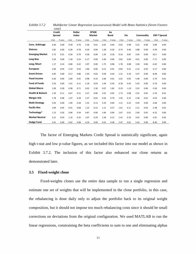
Exhibit 3.7.2 Multifactor Linear Regression (unconstrained) Model with Betas Statistics (Seven Factors

case)

Credit Spread

Dollar Index

SP500 Market

Aa Bond Vix Commodity EM-T Spread

t-Stat P-value t-Stat P-value t-Stat P-value t-Stat P-value t-Stat P-value t-Stat P-value t-Stat P-value

Conv. Arbitrage 6.40 0.00 0.39 0.70 2.58 0.01 6.65 0.00 0.02 0.98 3.52 0.00 -3.89 0.00

Distress 5.81 0.00 0.28 0.78 0.20 0.84 1.28 0.20 0.74 0.46 3.88 0.00 -5.94 0.00

Emerging Market 2.72 0.01 0.26 0.79 4.58 0.00 1.35 0.18 0.16 0.87 3.45 0.00 10.3 0.00

Long Bias 3.34 0.00 1.18 0.24 6.17 0.00 3.40 0.00 3.82 0.00 4.01 0.00 -7.71 0.00

Long /Short 1.17 0.24 0.80 0.42 3.97 0.00 1.75 0.08 1.78 0.08 3.58 0.00 -6.02 0.00

European 2.00 0.05 2.19 0.03 1.86 0.06 0.12 0.91 0.83 0.41 2.14 0.03 -4.17 0.00

Event Driven 4.05 0.00 0.17 0.86 2.44 0.02 0.58 0.56 1.31 0.19 3.47 0.00 -8.48 0.00

Fixed Income 6.20 0.00 2.00 0.05 0.98 0.33 2.66 0.01 2.01 0.05 5.48 0.00 -2.79 0.01

Fund of Funds 3.33 0.00 1.61 0.11 2.18 0.03 1.04 0.30 0.78 0.43 5.63 0.00 -5.76 0.00

Global Macro 1.09 0.28 0.38 0.71 0.02 2.30 0.07 1.82 0.19 -1.32 3.35 0.00 -3.50 0.00

Health & Biotech 1.59 0.11 0.67 0.51 3.37 0.00 2.01 0.05 1.73 0.08 2.01 0.05 -2.76 0.01

Merger Arb. 1.78 0.08 1.07 0.28 2.37 0.02 0.26 0.79 1.45 0.15 2.38 0.02 -4.93 0.00

Multi Strategy 5.03 0.00 1.09 0.28 1.52 0.13 5.33 0.00 1.21 0.23 4.93 0.00 -4.68 0.00

Pacific Rim 2.09 0.04 0.41 0.68 1.23 0.22 1.11 0.27 1.61 0.11 2.21 0.03 -2.38 0.02

Technology* 1.13 0.26 0.96 0.34 4.87 0.00 3.46 0.00 2.67 0.01 2.00 0.05 -4.22 0.00

Market Neutral 2.21 0.03 1.16 0.25 1.07 0.29 1.58 0.12 1.41 0.16 3.02 0.00 -2.01 0.05

Hedge Fund 3.41 0.00 0.02 0.98 4.29 0.00 0.55 0.58 2.47 0.01 5.43 0.00 -8.40 0.00

The factor of Emerging Markets Credit Spread is statistically significant, again

high t-stat and low p-value figures, as we included this factor into our model as shown in

Exhibit 3.7.2. The inclusion of this factor also enhanced our clone returns as

demonstrated later.

3.5 Fixed-weight clone

Fixed-weights clones use the entire data sample to run a single regression and

estimate one set of weights that will be implemented in the clone portfolio, in this case,

the rebalancing is done daily only to adjust the portfolio back to its original weight

composition, but it should not impose too much rebalancing costs since it should be small

corrections on deviations from the original configuration. We used MATLAB to run the

linear regressions, constraining the beta coefficients to sum to one and eliminating alphas

12

(intercepts). Since we are evaluating indexes and not specific funds, the human factor is

not as material and the elimination of alpha in our regression model does not result in a

relevant loss because of the aggregation effect of the indexes.

In our model the least squares algorithm R*it was applied using the factors’

means to fit the mean of the indexes. Later, we used the resulted estimated betas as the

representative weights for each factor and constructed each clone portfolio accordingly.

The constructed clone will have the returns that are equivalent to the fitted values

𝐸[R*it].

R*it = 𝛽∗𝑖1 𝑆𝑃𝑡 + 𝛽∗

𝑖2 𝐵𝑜𝑛𝑑𝑡 + 𝛽∗𝑖3 𝑉𝐼𝑋𝑡 + 𝛽∗

𝑖4 𝐶𝑀𝑇𝐷𝑌𝑡 + 𝛽∗𝑖 𝐶𝑅𝐸𝐷𝐼𝑇𝑡

𝐸[R*it] = 𝛼𝑖 + 𝛽𝑖1 𝐸[𝑆𝑃𝑡] + 𝛽𝑖2 𝐸[𝐵𝑜𝑛𝑑𝑡] + 𝛽𝑖3𝐸[𝑉𝐼𝑋𝑡]+ 𝛽𝑖4 𝐸[𝐶𝑀𝑇𝐷𝑌𝑡] + 𝛽𝑖[𝐶𝑅𝐸𝐷𝐼𝑇𝑡]

3.6 Rolling-windows clone

Rolling-windows clones use the data sample from a particular month-period to run

monthly regression and estimate a set of weights per month that will then be implemented

in the clone portfolio, the rebalancing in this case can be done monthly (or sparser

periodicity) to adjust the portfolio to the new set of weights, this case should impose

higher rebalancing costs compared to the fixed-weight clone strategy, since the weights

may diverge a lot from month to month.

Initially, we opted for 24-months rolling-windows following Hasanhodzic and Lo

(2006), that is, for each month t, we used the rolling-windows of 24-months from month

t-24 to t-1 to estimate the same regression as Rit-k.

The beta coefficients are indexed by both the k (period) and i (risk factors) and the

estimated betas 𝛽∗ are applied as weights to determine the returns of the constructed

clones R*it-k .

Rit-k = 𝛽𝑖1 𝑆𝑃𝑡−𝑘 + 𝛽𝑖2 𝐵𝑜𝑛𝑑𝑡−𝑘 + 𝛽𝑖3 𝑉𝐼𝑋𝑡−𝑘 + 𝛽𝑖4 𝐶𝑀𝑇𝐷𝑌𝑡−𝑘 + 𝛽𝑖 𝐶𝑅𝐸𝐷𝐼𝑇𝑡−𝑘 + 𝜀𝑖𝑡−𝑘

Subject to 1 = 𝛽𝑖1 + 𝛽𝑖2 + 𝛽𝑖3 + 𝛽𝑖4 + 𝛽𝑖 , k = 1, ... 24

R*it-k = 𝛽∗𝑖1 𝑆𝑃𝑡−𝑘 + 𝛽∗

𝑖2 𝐵𝑜𝑛𝑑𝑡−𝑘 + 𝛽∗𝑖3 𝑉𝐼𝑋𝑡−𝑘 + 𝛽∗

𝑖4 𝐶𝑀𝑇𝐷𝑌𝑡−𝑘 + 𝛽∗𝑖 𝐶𝑅𝐸𝐷𝐼𝑇𝑡−𝑘

+ 𝜀𝑖𝑡−𝑘

13

An important aspect, also described in Hasanhodzic and Lo (2006), is that fixed-

weight clones incur a clear look-ahead bias, since it uses the entire data sample to build

its portfolios. While rolling-windows estimations generates monthly rebalancing asset-

allocation weights for its clone-portfolios, controlling for biases and replicating features

of active management.

3.7 Rolling-windows calibration

After replicating Hasanhodzic and Lo (2006) models, we implemented a

sensitivity analysis on the rolling-windows model, relaxing the input parameter

attempting to improve the model replication capacity. The results appointed for an

optimal 12-months rolling-windows period.

Rit-k = 𝛽𝑖1 𝑆𝑃𝑡−𝑘 + 𝛽𝑖2 𝐵𝑜𝑛𝑑𝑡−𝑘 + 𝛽𝑖3 𝑉𝐼𝑋𝑡−𝑘 + 𝛽𝑖4 𝐶𝑀𝑇𝐷𝑌𝑡−𝑘 + 𝛽𝑖 𝐶𝑅𝐸𝐷𝐼𝑇𝑡−𝑘 + 𝜀𝑖𝑡−𝑘

Subject to 1 = 𝛽𝑖1 + 𝛽𝑖2 + 𝛽𝑖3 + 𝛽𝑖4 + 𝛽𝑖 , k=1, … 12

R**it-k = 𝛽∗∗𝑖1 𝑆𝑃𝑡−𝑘 + 𝛽∗∗

𝑖2 𝐵𝑜𝑛𝑑𝑡−𝑘 + 𝛽∗∗𝑖3 𝑉𝐼𝑋𝑡−𝑘 + 𝛽∗∗

𝑖4 𝐶𝑀𝑇𝐷𝑌𝑡−𝑘 + 𝛽∗∗𝑖 𝐶𝑅𝐸𝐷𝐼𝑇𝑡−𝑘

+ 𝜀𝑖𝑡−𝑘

Although the smaller rolling-windows period is subject to greater estimation

errors, market fast reaction imposes the need for this shorter window frame. In this stage,

we also relaxed the original factors by replacing and withdrawing each one of them.

Later, we tested for an additional strategy-specific factor to close the estimation gap and

improve the strategy-specific clone quality and accuracy. The results and intuitions

behind each model parameter will be further elaborated in the following chapter13

of this

study.

13

Chapter 4 Results, Model Calibration and Implications

14

4. Results, Model Calibration and Implications

Following Hasanhodzic and Lo (2006), we implemented two linear regression

models to perform a decomposition of each hedge fund strategy’s returns. We then based

our clone models on the results we got from the decomposition. For each model, we

calculated the mean returns and the standard deviation to have the insightful information

about our clone risk-return results and how they compared to the indexes. The statistical

measure of R-squared as shown on Exhibit 4.1 indicates the percentage of each particular

Barclay Index movements can be explained by each clone with different approach.

Exhibit 4.1 Summary of R-squared and F-test - (unconstrained model)

For example, the R-squared for the Global Macro strategy is the highest for the rolling

window of 12 months approach indicates the Barclay index of Global Macro strategy is

explained better by the clones, which used the rolling window of 12 months approach

compared with other approaches. The statistical results of R-squared and F-test after

incorporating the factor of Emerging Market Credit Spread is displayed on Exhibit 4.2.

R Squared Adjusted

R Squared

F-test R Squared Adjusted

R Squared

F-test R Squared Adjusted

R Squared

F-test

Conv. Arb. 0.472 0.459 36.0 0.285 0.282 93.2 0.323 0.320 106.0

Distressed* 0.471 0.457 35.7 0.343 0.340 122.0 0.469 0.467 196.0

Emer. Markets 0.455 0.442 33.6 0.515 0.513 249.0 0.545 0.542 265.0

Long Bias* 0.570 0.559 53.2 0.671 0.670 478.0 0.720 0.719 572.0

Long/Short 0.359 0.343 22.5 0.347 0.344 124.0 0.363 0.360 127.0

European* 0.223 0.203 11.5 0.104 0.101 27.3 0.138 0.134 35.6

Event Driven 0.481 0.468 37.2 0.401 0.398 157.0 0.473 0.471 200.0

Fixed Income Arb. 0.391 0.376 25.8 0.237 0.233 72.6 0.312 0.309 101.0

Fund of Funds 0.428 0.413 30.0 0.384 0.381 146.0 0.442 0.440 176.0

Global Macro 0.238 0.219 12.5 0.246 0.243 76.3 0.208 0.205 58.5

Health & Biotech* 0.221 0.201 11.4 0.076 0.072 19.1 0.080 0.076 19.2

Merger Arb. * 0.290 0.272 16.4 0.208 0.205 61.6 0.193 0.190 53.2

Multi Strategy 0.478 0.465 36.7 0.342 0.339 122.0 0.381 0.379 137.0

Pacific Rim* 0.204 0.184 10.3 0.140 0.137 38.2 0.130 0.126 233.1

Technology* 0.321 0.305 19.0 0.361 0.358 132.0 0.330 0.327 109.0

Market Neutral 0.085 0.062 3.7 0.049 0.044 11.9 0.036 0.032 8.4

Hedge Fund* 0.548 0.537 48.7 0.546 0.544 281.0 0.601 0.599 334.0

Fixed Weight 12-months Rolling Window 24-months Rolling Window

15

Exhibit 4.2 Summary of R-squared and F-test with Emerging Market Credit Spread- (unconstrained

model)

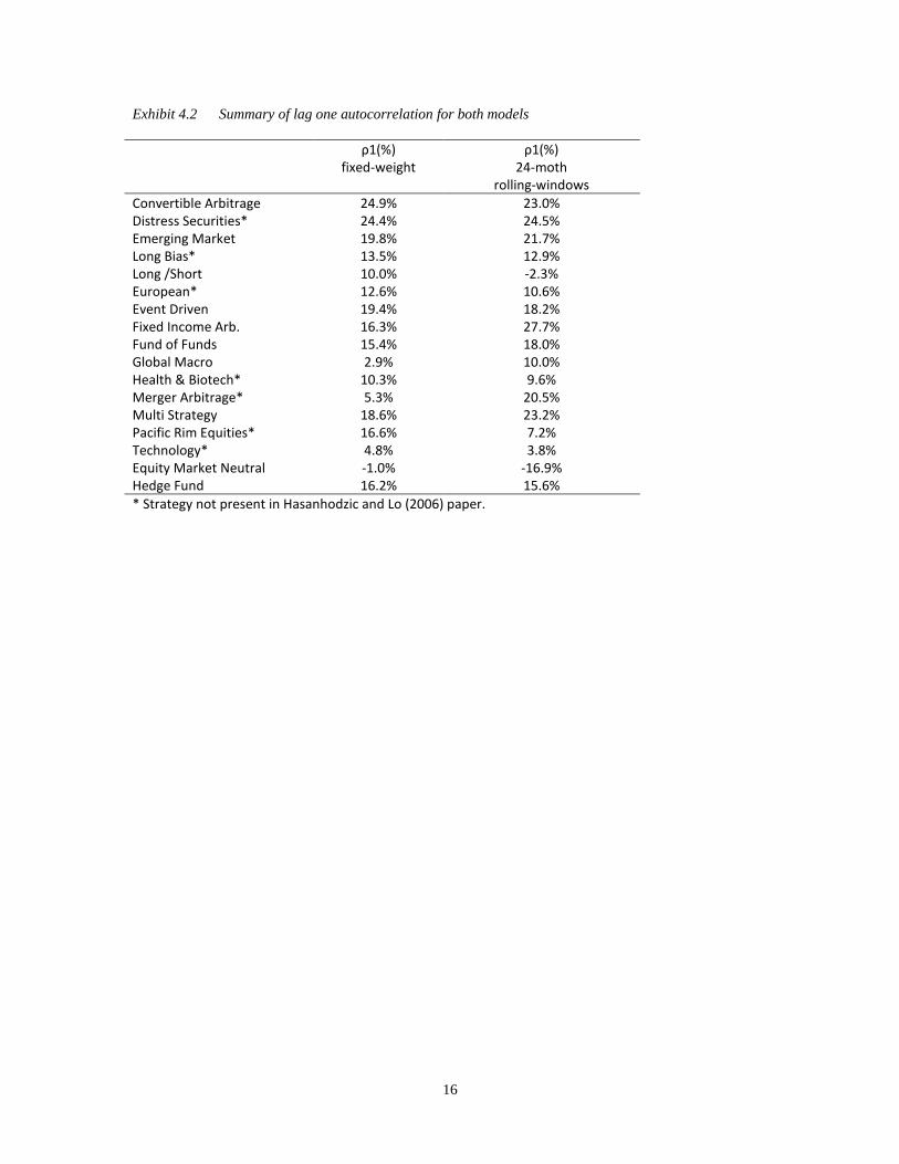
Meanwhile, we also applied the autocorrelation of lag one into our model to

assess the illiquidity risks as discussed in the study of Getmansky, Lo and Makarov that

the autocorrelation can be used to measure the illiquidity risk of the hedge funds (2004).

As different strategies have different rebalancing requirements, the clones perform

differently for different strategies and the performance of different types of clones also

varies. By using the approach of 24-months rolling-windows, most of the autocorrelation

of lag one decreased, which indicates a slightly declined liquidity risk due to the liquidity

improves under the embedded rebalancing requirements of the rolling window.

R Squared Adjusted R

Squared

F-test R Squared Adjusted

R Squared

F-test R Squared Adjusted

R Squared

F-test

Conv. Arb. 0.472 0.459 36.0 0.260 0.257 82.3 0.322 0.319 105.0

Distressed* 0.471 0.457 35.7 0.302 0.299 101.0 0.473 0.471 199.0

Emer. Markets 0.455 0.442 33.6 0.505 0.503 239.0 0.578 0.576 304.0

Long Bias* 0.570 0.559 53.2 0.632 0.630 402.0 0.712 0.711 549.0

Long/Short 0.359 0.343 22.5 0.315 0.312 108.0 0.340 0.337 114.0

European* 0.223 0.203 11.5 0.084 0.081 21.8 0.107 0.103 26.5

Event Driven 0.481 0.468 37.2 0.425 0.423 173.0 0.484 0.481 208.0

Fixed Income Arb. 0.391 0.376 25.8 0.230 0.227 69.8 0.322 0.319 106.0

Fund of Funds 0.428 0.413 30.0 0.351 0.348 126.0 0.437 0.434 172.0

Global Macro 0.238 0.219 12.5 0.248 0.245 77.1 0.202 0.198 56.2

Health & Biotech* 0.221 0.201 11.4 0.040 0.036 9.8 0.046 0.042 10.7

Merger Arb. * 0.290 0.272 16.4 0.185 0.182 53.2 0.191 0.188 52.5

Multi Strategy 0.478 0.465 36.7 0.295 0.292 97.9 0.382 0.379 137.0

Pacific Rim* 0.204 0.184 10.3 0.135 0.131 36.4 0.132 0.129 33.9

Technology* 0.321 0.305 19.0 0.264 0.260 83.7 0.278 0.274 85.3

Market Neutral 0.085 0.062 3.7 0.060 0.056 14.9 0.038 0.034 8.8

Hedge Fund* 0.548 0.537 48.7 0.516 0.514 250.0 0.594 0.592 324.0

Fixed Weight12-months Rolling Window

with EM Credit Spread

24-months Rolling Window

with EM Credit Spread

16

Exhibit 4.2 Summary of lag one autocorrelation for both models

ρ1(%) fixed-weight

ρ1(%) 24-moth

rolling-windows

Convertible Arbitrage 24.9% 23.0% Distress Securities* 24.4% 24.5% Emerging Market 19.8% 21.7% Long Bias* 13.5% 12.9% Long /Short 10.0% -2.3% European* 12.6% 10.6% Event Driven 19.4% 18.2% Fixed Income Arb. 16.3% 27.7% Fund of Funds 15.4% 18.0% Global Macro 2.9% 10.0% Health & Biotech* 10.3% 9.6% Merger Arbitrage* 5.3% 20.5% Multi Strategy 18.6% 23.2% Pacific Rim Equities* 16.6% 7.2% Technology* 4.8% 3.8% Equity Market Neutral -1.0% -16.9% Hedge Fund 16.2% 15.6%

* Strategy not present in Hasanhodzic and Lo (2006) paper.

17

Exhibit 4.3 Summary of 1 dollar invested accumulated return for 24-months rolling-windows monthly

rebalancing clone portfolios, fixed-weight clone portfolios and Barclay Hedge Indexes. The

clones were obtained by linear regressions of monthly returns of Barclay Hedge Indexes

from January 1997 to August 2017 on six factors: S&P 500 total return, Barclays Aa

Corporate Total Return Index, the US Dollar Index return, Credit Spread: US Corporate

Baa - 10-year US Treasury, the first-difference of the CBOE Volatility Index (VIX), and the

Goldman Sachs Commodity Index (GSCI) total return.

Exhibit 4.4 Individual charts of the same data displayed in the summary of Exhibit 4.2

18

24-Moths Rolling-Windows Clone Fixed-Weight Clone Barclay Hedge Index

19

24-Moths Rolling-Windows Clone Fixed-Weight Clone Barclay Hedge Index

20

Exhibit 4.5 Clones’ Statistics & Tracking Errors (Data sample from January 1998 to August 2017)

24-months Rolling-Window Fixed-Weight

Strategy E(R)

Index

STD

Index

E(R)

R-W

STD

R-W

Tracking

Error RW

E(R)

F-W

STD

F-W

Tracking

Error FW

Conv. Arb. 6.7% 6.3% 4.4% 5.4% 5.6% 4.3% 5.0% 4.8%

Distressed* 7.9% 6.9% 5.4% 6.6% 5.4% 3.7% 5.8% 5.3%

Emer. Markets 10.0% 12.4% 5.8% 12.5% 9.1% 4.4% 10.5% 8.0%

Long Bias* 8.4% 10.5% 4.8% 10.5% 5.9% 3.9% 10.0% 5.2%

Long/Short 7.7% 6.4% 3.6% 6.4% 5.8% 3.3% 5.4% 5.0%

European* 8.4% 7.1% 3.2% 6.2% 7.6% 3.4% 4.7% 6.4%

Event Driven 8.3% 6.0% 4.8% 6.2% 4.9% 3.7% 5.7% 4.5%

Fixed Income Arb. 5.7% 5.0% 3.5% 4.8% 4.6% 3.5% 4.1% 4.1%

Fund of Funds 4.5% 5.1% 3.6% 5.6% 4.4% 3.4% 4.5% 4.0%

Global Macro 6.3% 5.1% 4.2% 5.5% 5.6% 3.6% 3.7% 4.8%

Health & Biotech* 13.3% 15.6% 5.4% 11.2% 16.6% 3.5% 8.3% 14.2%

Merger Arb. * 6.9% 3.1% 3.0% 4.0% 4.0% 3.3% 3.3% 3.5%

Multi Strategy 7.8% 4.4% 4.0% 4.7% 4.1% 3.8% 4.1% 3.7%

Pacific Rim* 8.6% 8.5% 2.7% 7.2% 9.1% 3.4% 5.3% 7.6%

Technology* 9.4% 12.1% 2.7% 11.5% 11.1% 3.0% 8.4% 9.7%

Market Neutral 4.4% 2.8% 2.7% 3.8% 4.3% 3.0% 2.8% 3.8%

Hedge Fund* 7.9% 6.6% 4.2% 6.9% 4.6% 3.7% 6.2% 4.1%

Average 7.8% 7.3% 4.0% 7.0% 6.6% 3.6% 5.8% 5.8%

*Strategy not present in Hasanhodzic and Lo (2006) paper.

Although the data source and time-period were quite distinct, the quality of the

replications obtained by the 24-months rolling-windows clones was similar to the 24-

months rolling-windows clones of the original study conducted by Hasanhodzic and Lo

(2006). Nevertheless, in our opinion this replication is not of enough quality to justify the

strategy, considering that current market conditions provide investors with much lower

returns and, as demonstrated by Exhibit 4.4, the clones underperform the indexes by a

very significant amount.

Regarding the fixed-weight linear clones, in our time-frame and data, the results

obtained were similar to those of the 24-months rolling-windows linear clones, diverging

the findings from Hasanhodzic and Lo (2006). Our interpretation is that the sub-prime

21

crisis brought a structural break point14

in our data set; consequently, our entire-period

regressions do not provide as precise weights as the original Hasanhodzic and Lo (2006)

study.

As mentioned before because fixed-weight clones incur from look-ahead bias and

will not react in changes to market conditions, we believe that rolling-windows

estimations are more applicable, as it generates monthly rebalancing asset-allocation

weights for its clone-portfolios, controlling for biases and replicating features of active

management. Also, this model will avoid issues related to possible structural breaks that

may occur.

4.1 Other periods rolling-windows

After this exercise, we started to conduct experimentation in order to calibrate this

original 24-months rolling-windows model. The first effort was changing the periodicity

of the rebalancing of the rolling-windows portfolios to more sparse periods. The results

were the deterioration of the clones’ ability to replicate the original trends observed by

the indexes, therefore we continued to use monthly rebalancing. Next, we attempt for

different timespan in the rolling-windows linear regressions, again periods larger than 24-

months resulted in a deterioration of the clones, so we decided to test smaller periods.

For most strategies, the autocorrelations for the fixed-weight clones are the

highest and the 12-months rolling-windows clones are the lowest. These results indicate

that the liquidity risk decreases using a smaller timespan in the rolling-windows model

(see Exhibit 4.1.1 below).

14

When the data have a dramatic event that changes the dynamics of the time-series behaviour and one

single linear model cannot successfully fit the entire period with a single regression equation.

22

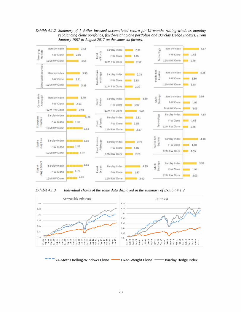
Considering the accumulated returns and observing the charts below, the 12-

months rolling-windows results were an impressive improvement from the original 24-

months period, yielding higher returns for all strategies. On the other hand, this new

method had a deterioration in tracking error metric and showed a larger volatility (see

Exhibit 4.1.2 and 4.1.3 below).

4.1.1 Summary of lag one autocorrelation for the three models

ρ1(%) fixed-weight

ρ1(%) 24-months R-W

ρ1(%) 12-moths R-W

Convertible Arbitrage 24.9% 23.0% 3.4% Distress Securities 24.4% 24.5% 14.2% Emerging Market 19.8% 21.7% 15.7% Long Bias 13.5% 12.9% 5.5% Long /Short 10.0% -2.3% -5.5% European 12.6% 10.6% 2.3% Event Driven 19.4% 18.2% 8.7% Fixed Income Arb. 16.3% 27.7% 14.0% Fund of Funds 15.4% 18.0% 6.8% Global Macro 2.9% 10.0% 8.9% Health & Biotech 10.3% 9.6% -2.9% Merger Arb. 5.3% 20.5% 11.7% Multi Strategy 18.6% 23.2% 14.1% Pacific Rim Equities* 16.6% 7.2% 21.2% Technology* 4.8% 3.8% 4.4% Equity Market Neutral -1.0% -16.9% -17.1% Hedge Fund 16.2% 15.6% 8.9%

23

Exhibit 4.1.2 Summary of 1 dollar invested accumulated return for 12-months rolling-windows monthly

rebalancing clone portfolios, fixed-weight clone portfolios and Barclay Hedge Indexes. From

January 1997 to August 2017 on the same six factors.

Exhibit 4.1.3 Individual charts of the same data displayed in the summary of Exhibit 4.1.2

24-Moths Rolling-Windows Clone Fixed-Weight Clone Barclay Hedge Index

24

24-Moths Rolling-Windows Clone Fixed-Weight Clone Barclay Hedge Index

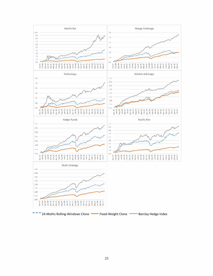
25

24-Moths Rolling-Windows Clone Fixed-Weight Clone Barclay Hedge Index

26

Exhibit 4.1.4 Clones’ Statistics & Tracking Errors with 24-months and 12-months RW (Data sample from January 1998 to August 2017)

12-months Rolling-Window 24-months Rolling-Window

Conv. Arb. E(R)

Index STD

Index E(R) R-W

STD R-W

Tracking Error RW

E(R) R-W

STD R-W

Tracking Error RW

Covert. Arb. 6.7% 6.3% 6.0% 6.5% 6.1% 4.4% 5.4% 5.6% Distressed* 8.0% 6.9% 7.4% 7.7% 6.5% 5.4% 6.6% 5.4% Emer. Markets 10.0% 12.4% 9.6% 12.8% 9.7% 5.8% 12.5% 9.1% Long Bias* 8.4% 10.5% 7.3% 10.9% 6.7% 4.8% 10.5% 5.9% Long/Short 7.7% 6.4% 6.0% 7.3% 6.5% 3.6% 6.4% 5.8% European* 8.4% 7.1% 7.3% 7.5% 8.3% 3.2% 6.2% 7.6% Event Driven 8.3% 6.0% 6.7% 7.3% 5.8% 4.8% 6.2% 4.9% FI Arb. 5.7% 5.0% 4.5% 5.4% 5.2% 3.5% 4.8% 4.6% Fund of Funds 4.5% 5.1% 5.4% 6.1% 5.0% 3.6% 5.6% 4.4% Global Macro 6.3% 5.1% 5.2% 6.5% 6.1% 4.2% 5.5% 5.6% Health & Biotech* 13.3% 15.6% 9.4% 14.6% 19.8% 5.4% 11.2% 16.6% Merger Arb. * 6.9% 3.1% 3.4% 4.8% 4.5% 3.0% 4.0% 4.0% Multi Strategy 7.8% 4.4% 5.9% 5.4% 4.5% 4.0% 4.7% 4.1% Pacific Rim* 8.6% 8.5% 6.7% 10.0% 9.9% 2.7% 7.2% 9.1% Technology* 9.4% 12.1% 6.5% 12.6% 11.5% 2.7% 11.5% 11.1% Market Neutral 4.4% 2.8% 3.2% 4.4% 4.7% 2.7% 3.8% 4.3% Hedge Fund* 7.9% 6.6% 6.3% 7.5% 5.3% 4.2% 6.9% 4.6%

Average 7.8% 7.3% 6.3% 8.1% 7.4% 4.0% 7.0% 6.6%

*Strategy not present in Hasanhodzic and Lo (2006) paper.

Looking at the exhibits above, although there was a deterioration in the tracking

error metrics, the improvement in expected returns was expressive and seems like a

reasonable trade-off and an overall improvement in the model to change 24-months for

12-months rolling-windows. Though the new clones present larger volatilities (STD =

annualized standard deviation), these figures are very similar to the index volatilities, so

an investor should be somewhat comfortable with this level of risk. Because many

strategies are quite specific15

we did not expect all clones to show consistently accurate

replications. In our point of view to further calibrate the model, it is imperative to

understand the specific strategy and research specific additional factors relevant to that

strategy. Therefore, we decided to choose one Global Macro strategy for a more in-depth

model building.

15

Refer to Appendix A. Strategy Definitions for the detailing of strategies.

27

5. Global Macro Strategy - A Study Case

The reasoning behind our focus in Global Macro hedge fund strategy replication

is mainly its capacity of preserving capital through a low correlation with the main

indexes of variable income and fixed income, its mandate is the broadest hedge funds and

has no formal definition due to its opportunistic nature. Another convenient fact is that

this strategy can be used on very large amounts under management as it focuses in very

liquid markets, with an emphasis in currency trading usually.

Exhibit 5.1 Yearly Returns of the Barclay Hedge Macro Index from 1997 to August 2017.

Typically, a Global Macro manager aims to obtain positive absolute return

adjusted to a certain level of risk under any market circumstances. For this, it takes

positions directional (bearish or bullish) or non-directional with or without financial

leverage and using any instrument, whether liquid or derivative in the foreign exchange

markets, interest rates, variable income, commodities and exceptionally risk capital. The

main source of return generation is the analysis of situations of macroeconomic

disequilibrium fundamental in any international market.

28

The Exhibit 5.3 below shows the detailing of the 12-month rolling-windows

monthly rebalance strategy obtained by the 6 factors regression; it is quite intuitive to see

how this process was able to capture the managers’ insights in an opportune and

consistent system. Global Macro strategy had a superior comparative performance to

most asset classes in downturn years and in our 12-months rolling-windows strategy you

can see the translation from the managers knowledge into our model as the disinvestment

in S&P 500 starts around 2008’s first quarter, before the S&P vast drawdown, and most

of the portfolio market share is taken by Aa Corporate Total Return Index.

Exhibit 5.2 Yearly Returns of the Clone 12-months rolling-windows with the 6-factor model

14% 15%

2% 5%

10% 7%

3% 5%

9%

-17%

6% 7% 5% 5%

10% 8%

0% 4% 4%

1999 2000 2001 2002 2003 2004 2005 2006 2007 2008 2009 2010 2011 2012 2013 2014 2015 2016 2017*

12-months RW 6-factors Clone Historical Data

Clone Index

29

Exh

ibit 5

.3

Su

mm

ary

of

1

do

llar

invested

a

ccum

ula

ted

return

fo

r 12

m

on

ths

rollin

g-w

ind

ow

m

on

thly

reba

lan

cing

po

rtfolio

s a

nd

fixed-w

eight

po

rtfolio

s. Ob

tain

ed b

y linea

r regressio

ns o

f mo

nth

ly return

s of h

edg

e fun

ds in

the B

arcla

y Hed

ge In

dexes fro

m Ja

nu

ary 1

99

9 to

Au

gu

st

20

17 o

n six fa

ctors: S

&P

50

0 to

tal retu

rn, A

A B

on

d In

dex retu

rn, th

e US D

olla

r Ind

ex return

, the sp

read

betw

een th

e US

Agg

reg

ate L

ong

Cred

it BA

A B

on

d In

dex a

nd th

e Trea

sury L

on

g In

dex, th

e first-differen

ce of th

e CB

OE

Vo

latility In

dex (V

IX), a

nd

the G

old

ma

n S

ach

s

Co

mm

od

ity Ind

ex (GS

CI).

30

5.1 Factor selection

George Soros, one of the most famous investors of all times is adept at Global

Macro strategy. Three of his most successful trades of all his track-record related to

macro international critic turning points and took the form of currency bets: He shorted

the Pound in 1992, profiting from the fall of the European Exchange Rate Mechanism; he

successfully shorted the Malaysian Baht in the Asian financial crisis of 1997; and most

recently in 2013 and 2014, he shorted the Yen taking profits out of president Abe’s

quantitative easing program the deteriorated Japan’s currency16

.

Although the Dollar Index provides a decent proxy for currency trades, because of

its composition, we thought that this original six-factors-model was missing the

Emerging Markets specific-effect. Currently, the Dollar Index is calculated by factoring

in the exchange rates of six major world currencies the Euro (EUR), roughly 8% weight,

Japanese yen (JPY), roughly 14% weight, Pound sterling (GBP), roughly 12% weight,

Canadian dollar (CAD), roughly 9% weight, Swedish krona (SEK), roughly 4% weight

and Swiss franc (CHF), roughly 4% weight17

.

The commodity factor also brings some indirect exposure to Emerging Markets

trends, but the commodity market affects the emerging market countries much more than

it is affected by them, so it is not heavily influenced by idiosyncratic risk and overall risk

aversion. To better capture the Emerging Market specific-effect in a consistent and

extremely liquid manner we turned to the sovereign debt market of Emerging Markets

countries. The debt market is the best thermometer for these countries because of its

liquidity and size liquidity, far superior to its stock exchanges.

16

Wikipedia December 2017 17

Investopedia December 2017

31

Also, the debt market has a contamination effect that helps the replication strategy

to better absorb global market opportunities. As an example, when Russia defaulted in

1998, the Brazilian currency suffered a strong speculation attack that reflected in

Brazilian sovereign debt instantly and with high intensity, the Dollar Index and

Commodity index did not get affected in the same speed and intensity as the Emerging

Market debt index.

Exhibit 5.1.1 Monthly Returns of Dollar Index, Commodity, and Emerging Market - Treasury

For those reasons, we opted for the J.P. Morgan EMBI Diversified Sovereign

Spread (JPEIDISP) Index, that captures the spread return results from the yield difference

between emerging markets debt and US treasuries and has more than twenty years of

track-record. The results obtained after the addition of this seventh factor was almost

imperceptible in the fixed-weight regression model, but in the 12-months rolling-

windows monthly-rebalancing model clones, it significantly improved the quality of the

returns replication.

-30%

-10%

10%

30%

50%

70%

Mar

-98

Ap

r-9

8

May

-98

Jun

-98

Jul-

98

Au

g-9

8

Sep

-98

Oct

-98

No

v-9

8

De

c-9

8

Jan

-99

Feb

-99

Mar

-99

Ap

r-9

9

May

-99

Jun

-99

Jul-

99

Au

g-9

9

Sep

-99

Oct

-99

No

v-9

9

Mar 1998 to Nov 1999 Monthly Returns

US_Dollar_Index COMDTY Sov Emerging Market - Treasury Spread

32

Exh

ibit 5

.1.2

S

um

ma

ry o

f 1

d

olla

r in

vested

accu

mu

lated

retu

rn

for

12

m

on

ths

rollin

g-w

ind

ow

m

on

thly

reba

lan

cing

p

ortfo

lios,

fixed-w

eigh

t

po

rtfolio

s an

d B

arcla

y Hed

ge In

dexes. O

bta

ined

by lin

ear reg

ression

s of m

on

thly retu

rns o

f hed

ge fu

nd

s in th

e Ba

rclay H

edg

e Ind

exes

from

Jan

ua

ry 19

99 to

Au

gu

st 20

17

on

seven fa

ctors: S

&P

50

0 to

tal retu

rn, A

A B

on

d In

dex retu

rn, th

e US

Do

llar In

dex retu

rn, th

e

sprea

d b

etween

the U

S A

gg

rega

te Lo

ng

Cre

dit B

AA

Bo

nd

Ind

ex an

d th

e Trea

sury L

on

g In

dex, th

e first-differen

ce of th

e CB

OE

Vo

latility In

dex (V

IX), th

e Gold

ma

n S

ach

s Co

mm

od

ity Index (G

SC

I) tota

l return

, an

d th

e J.P. M

org

an E

MB

I Diversified

So

vereign

Sp

read

(JPE

IDIS

P) In

dex

33

Exh

ibit 5

.1.3

S

um

ma

ry o

f 1

d

olla

r in

vested

accu

mu

lated

retu

rn

for

12

m

on

ths

rollin

g-w

ind

ow

m

on

thly

reba

lan

cing

p

ortfo

lios

an

d

fixed-w

eigh

t

po

rtfolio

s. Ob

tain

ed b

y linea

r regressio

ns o

f mo

nth

ly return

s of h

edg

e fun

ds in

the B

arcla

y Hed

ge In

dexes fro

m Ja

nua

ry 19

99

to A

ugu

st

20

17 o

n six fa

ctors: S

&P

50

0 to

tal retu

rn, A

A B

on

d In

dex retu

rn, th

e US D

olla

r Ind

ex return

, the sp

read

betw

een th

e US

Agg

reg

ate L

ong

Cred

it BA

A B

on

d In

dex a

nd

the T

reasu

ry Lo

ng

Ind

ex, the first-d

ifference o

f the C

BO

E V

ola

tility Ind

ex (VIX

), an

d th

e Go

ldm

an

Sa

chs

Co

mm

od

ity Ind

ex (GS

CI) to

tal retu

rn a

nd

the J.P

. Mo

rga

n E

MB

I Diversified

So

vereign

Sp

read

(JPE

IDIS

P) In

dex.

34

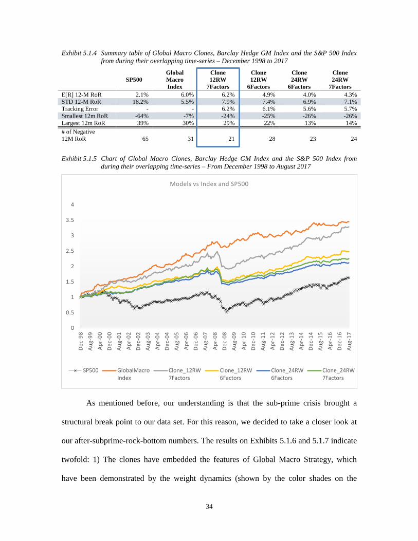
Exhibit 5.1.4 Summary table of Global Macro Clones, Barclay Hedge GM Index and the S&P 500 Index

from during their overlapping time-series – December 1998 to 2017

SP500

Global

Macro

Index

Clone

12RW

7Factors

Clone

12RW

6Factors

Clone

24RW

6Factors

Clone

24RW

7Factors

E[R] 12-M RoR 2.1% 6.0% 6.2% 4.9% 4.0% 4.3%

STD 12-M RoR 18.2% 5.5% 7.9% 7.4% 6.9% 7.1%

Tracking Error - - 6.2% 6.1% 5.6% 5.7%

Smallest 12m RoR -64% -7% -24% -25% -26% -26%

Largest 12m RoR 39% 30% 29% 22% 13% 14%

# of Negative

12M RoR 65 31 21 28 23 24

Exhibit 5.1.5 Chart of Global Macro Clones, Barclay Hedge GM Index and the S&P 500 Index from

during their overlapping time-series – From December 1998 to August 2017

As mentioned before, our understanding is that the sub-prime crisis brought a

structural break point to our data set. For this reason, we decided to take a closer look at

our after-subprime-rock-bottom numbers. The results on Exhibits 5.1.6 and 5.1.7 indicate

twofold: 1) The clones have embedded the features of Global Macro Strategy, which

have been demonstrated by the weight dynamics (shown by the color shades on the

0

0.5

1

1.5

2

2.5

3

3.5

4

De

c-9

8

Au

g-9

9

Ap

r-0

0

De

c-0

0

Au

g-0

1

Ap

r-0

2

De

c-0

2

Au

g-0

3

Ap

r-0

4

De

c-0

4

Au

g-0

5

Ap

r-0

6

De

c-0

6

Au

g-0

7

Ap

r-0

8

De

c-0

8

Au

g-0

9

Ap

r-1

0

De

c-1

0

Au

g-1

1

Ap

r-1

2

De

c-1

2

Au

g-1

3

Ap

r-1

4

De

c-1

4

Au

g-1

5

Ap

r-1

6

De

c-1

6

Au

g-1

7

Models vs Index and SP500

SP500 GlobalMacroIndex

Clone_12RW7Factors

Clone_12RW6Factors

Clone_24RW6Factors

Clone_24RW7Factors

35

graph). As can be seen from the graph, the blue shade (represents the weight allocating in

SP500) got almost vanished on July of 2008, which is prior to the financial crisis. As the

Global Macro Strategy features in betting on the big event, the quick response of the

clone to the market indicated by the weights shows a good replication. 2) The clones

outperformed the Global Macro Barclay Hedge Index by more than 3% p.a. while

maintaining a lower standard deviation, a lower worst 12-months rolling-windows

drawdown and less 12-months rolling-windows negative returns.

Exhibit 5.1.6 Chart of $1-dollar investment in Global Macro Clones, Barclay Hedge GM Index and the

S&P 500 Index from during their overlapping time-series – From October 2009 to August

2017

Exhibit 5.1.7 Summary table of Global Macro Clones, Barclay Hedge GM Index and the S&P 500 Index

from during their overlapping time-series – March2009 to August 2017

SP500

Global

Macro

Index

Clone 12RW

7 Factors Clone 12RW

6 Factors

Clone 24RW

6 Factors

Clone

24RW

7 Factors

E[R] 12-M RoR 10.2% 2.6% 6.0% 5.6% 4.6% 4.7%

STD 12-M RoR 7.8% 3.1% 3.0% 2.9% 2.4% 2.5%

Tracking Error - - 4.2% 4.4% 3.3% 3.4%

Smallest 12m RoR -9.3% -3.8% -2.3% -2.8% -1.0% -0.9%

Largest 12m RoR 15.3% 8.9% 12.58% 12.1% 9.8% 9.7%

#of Negative

12M RoR 12 22 3 3 4 5

0.80

1.30

1.80

2.30

2.80

Ap

r-0

9

Jul-

09

Oct

-09

Jan

-10

Ap

r-1

0

Jul-

10

Oct

-10

Jan

-11

Ap

r-1

1

Jul-

11

Oct

-11

Jan

-12

Ap

r-1

2

Jul-

12

Oct

-12

Jan

-13

Ap

r-1

3

Jul-

13

Oct

-13

Jan

-14

Ap

r-1

4

Jul-

14

Oct

-14

Jan

-15

Ap

r-1

5

Jul-

15

Oct

-15

Jan

-16

Ap

r-1

6

Jul-

16

Oct

-16

Jan

-17

Ap

r-1

7

Jul-

17

Models vs Index Pos 2008-Crisis World

SP500 GlobalMacroIndex

Clone_12RW7Factors

Clone_12RW6Factors

Clone_24RW6Factors

Clone_24RW7Factors

36

Exhibit 5.1.8 Yearly Returns of the Clone 12-months rolling-windows with the 7-factor model January

1999 to August 2017

We believe that the massive liquidity increases after quantitative easing programs

and the flatter yield curve and its compressed spreads are stealing performance from

complex models and expensive fee structures and beneficiating our clones’ semi-passive

strategy. Another relevant observation is that the clones of this study do not account for

any transactional or operational costs, but considering the available indices trackers in the

market and the competitive costs that a large institutional client have access to, we

believe that this over performance is more than enough to absorb these costs.

16% 22%

6% 5% 11% 9%

3% 9% 10%

-15%

6% 8% 4% 4%

8% 10%

1% 6% 5%

1999 2000 2001 2002 2003 2004 2005 2006 2007 2008 2009 2010 2011 2012 2013 2014 2015 2016 2017*

Enhanced Clone vs Barclay Global Macro Index

Clone Index

37

6. Conclusion

The linear regression model is a simple but meaningful tool that enables us to

quickly study the fund performance by decomposing the returns, especially for the funds

that have exposures to different and broad risk factors. As pointed out by Hasanhodzic

and Lo (2006), the factor-model method is a process of reverse-engineering of a hedge

fund strategy, in a way, profiting from the intellectual efforts embedded to the funds that

compose an index.

We based our study on the paper of Hasanhodzic and Lo (2006) and applied the

same methodology with the updated data to examine the performance of the hedge fund.

Hasanhodzic and Lo (2006) concluded that a fixed-weight model yields a better historical

performance compared to a rolling-windows model. While our conclusion analyzing a

different data set is the opposite, our results led us to the conclusion that the fixed-weight

method yields a similar historical performance as the rolling-windows of 24 months most

of the time (10 out of 17 strategies).

The 12-months rolling-windows approach shows a better replication for most

strategies, yielding closer results to the indexes. The discrepancy between our conclusion

and the conclusion from Hasanhodzic and Lo (2006) might have resulted from the

differences in the dataset, as our data includes several critical financial events that require

a more frequent rebalance with an asset-class allocation review, which is embedded in the

rolling-windows model.

Although the results from the rolling window of 12-months approach show

improvement, investors still need to carefully assess each strategy and make

experimentations to the model in order to improve it before applying the replication

38

method in practice. In our study, motivated by the paper of Hasanhodzic and Lo (2006),

we incorporated a new factor that we believe was missing in the original model and it is

very relevant to the Global Macro strategy: The Emerging Market Debt Credit Spread.

The improved model returned an enhanced back-testing performance, which brought us

further interesting findings: 1) The linear regression does not fully replicate the hedge

fund performance, but mimics the hedge fund strategies to a reasonable degree, especially

when the model expands the universe of factors by including a proper strategy-specific

risk factor; 2) the rolling window of 12-months approach combined with the strategy-

specific factor returns an even more practical way of replicating the Global Macro

Strategy; 3) considering the enhanced model back-testing performance our Global Macro

clone could still outperform the index and it could prove to be more beneficial to the

investors because of its semi-passive features, even if we account for transaction costs

and operational fees.

There are certain boundaries to our study, especially because linear regressions

multi-factor models do not fully capture the performance of the hedge fund strategies as

there are also uncaptured non-linear factors in hedge funds returns. The study done by

Dimitrios Giannikis (2011) has proven that there are different non-linear risk exposures

of hedge funds to different risk factors, and this nonlinearity appears to the different risk

factors rather than the market. By ignoring the presence of non-linearity associated with

non-linear risk-factors will result in “misleading conclusion about ‘alpha’ and about the

risk exposures of hedge funds.”18

Therefore, a further study should be conducted to

incorporate the non-linear factors to the model. Other Improvements that should be

18

Dimitrios Giannikis (2011)

39

considered in an extension of this study are: 1) The implementation of a cap for a

maximum amount of leverage to guarantee the feasibility of the strategy implementation;

2) Attempt for an implementation strategy using available ETFs and account for all

operational costs.

40

Appendices

41

Appendix A

42

1. Strategy Definitions

1.1 Barclay Hedge Indexes

The following is a list of category descriptions taken directly from Barclay Hedge

documentation, that define the criteria used by Barclay Hedge in assigning funds in

their database to one of the 17 possible categories. In their documentation it is also

highlighted for each strategy that only funds that provide net returns are included

in the index calculation.

1.2 Barclay Convertible Arbitrage Index

1.3 Barclay Distressed Securities Index

1.4 Barclay Emerging Markets Index

43

1.5 Barclay Equity Long Bias Index

1.6 Barclay Equity Long/Short Index

1.7 Barclay Equity Market Neutral Index

1.8 Barclay European Equities Index

1.9 Barclay Event Driven Index

44

1.10 Barclay Fixed Income Arbitrage Index

1.11 Barclay Fund of Funds Index

1.12 Barclay Global Macro Index

1.13 Barclay Healthcare & Biotechnology Index

45

1.14 Barclay Merger Arbitrage Index

1.15 Barclay Multi Strategy Index

1.16 Barclay Pacific Rim Equities Index

1.17 Barclay Technology Index

46

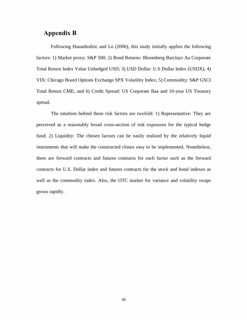
Appendix B

Following Hasanhodzic and Lo (2006), this study initially applies the following

factors: 1) Market proxy: S&P 500; 2) Bond Returns: Bloomberg Barclays Aa Corporate

Total Return Index Value Unhedged USD; 3) USD Dollar: U.S Dollar Index (USDX); 4)

VIX: Chicago Board Options Exchange SPX Volatility Index; 5) Commodity: S&P GSCI

Total Return CME; and 6) Credit Spread: US Corporate Baa and 10-year US Treasury

spread.

The intuition behind these risk factors are twofold: 1) Representative: They are

perceived as a reasonably broad cross-section of risk exposures for the typical hedge

fund; 2) Liquidity: The chosen factors can be easily realized by the relatively liquid

instruments that will make the constructed clones easy to be implemented. Nonetheless,

there are forward contracts and futures contracts for each factor such as the forward

contracts for U.S. Dollar index and futures contracts for the stock and bond indexes as

well as the commodity index. Also, the OTC market for variance and volatility swaps

grows rapidly.

47

Bibliography

Hasanhodzic, J. and Lo, A. (2006b). “Can Hedge-Fund Returns Be Replicated?: The Linear

Case”, The Journal of Investment Management, Vol. , No. 2, (2007), pp. –4.

Kamal Suppal (2004) “Constructing Multi-Strategy Fund Of Hedge Funds”, Global Asset

and Wealth Management Program - Simon Frasier University

Stephane Meng-Feng Yena, Ying-Lin Hsub and Yi-Long Hsiao (2014). “Can hedge fund

elites consistently beat the benchmark? A study of portfolio Optimization”, Asia

Pacific Management Review

William Fung and David A. Hsieh (1997). “Empirical Characteristics of Dynamic Trading

Strategies: The Case of Hedge Funds”, The Review of Financial Studies, Vol 10,

No. 2 (Summer,1997) , pp. 27-302.

Richerd M. Ennis (2007). “Editor’s Corner: Hedge Fund Clones: Triumph of Form over

Substance?” Financial Analysts Journal, Vol. 63, No. 3 (May-Jun., 2007), pp. 6-7.

Omar Naser (2007),“Replicating Hedge Fund Returns: A Factor Model Approach”,

Masters of Financial Risk Management Program - Simon Frasier University

M. Teresa Corzo-Santamaría, Jorge Martin-Hidalgo and Margarita Prat-Rodrigo (2014).

“Hedge Funds Global Macro Y Su Incorporación En Carteras De Activos

Tradicionales”, Universia Business Review | Segundo Trimestre 2014 | Issn:

1698-117

Getmansky, M., Lo, A., & Makarov, I. (2004, July). An econometric model of serial

correlation and illiquidity in hedge fund returns. Journal of Financial Economics.

Amenc, N., Martellini, L., Meyfredi, J.-C., & Ziemann, V. (2010). Passive Hedge Fund

Replication - Beyond the Linear Case. European Financial Management, 16(2),

191-210.

Basel Committee on Banking Supervision (BCBS). (2013). Basel III: The Liquidity Coverage

Ratio and liquidity risk monitoring tools.

Basel Committee on Banking Supervision (BCBS). (2016). Interest rate risk in the banking

book.

48

Carhart, M. M. (1997, March). On Persistence in Mutual Fund Performance. The Journal

of Finance, 1540-6261.

Dimitrios Giannikis, I. D. (2011). A Bayesian approach to detecting nonlinear risk

exposures in hedge fund strategies. Journal of Banking & Finance, 1399-1414.

Dimitrios Stafylas, K. A. (2017). Recent advances in explaining hedge fund returns:

Implicit factors and exposures. Global Finance Journal, 69-87.

Fama, E. F., & French, K. R. (1993, February). Common risk factors in the returns on

stocks and bonds. Journal of Financial Economics, 3-56.

Financial Institutions Commission (FICOM). (1990). Financial Institutions Act.

Getmansky, M., Lo, A., & Makarov, I. (2004, July). An econometric model of serial

correlation and illiquidity in hedge fund returns. Journal of Financial Economics.

Jasmina Hasanhodzic, A. W. (2007). Can Hedge-Fund returns be replicated?: The Linear

Case. Journal of Investment Management, 41.

Jorion, P. (2002). How Informative Are Value-at-Risk Disclosures? The Accounting

Review, 77(4), 911-931.

Michael S. O'Doherty, N. A. (2017). Hedge Fund Replication: A Model Combination

Approach. Review of Finance, 1767-1804.

Narasimhan, J., & Titman, S. (1993, March ). Returns to Buying Winners and Selling

Losers: Implications for Stock Market Efficiency. The Journal of Finance, 1540-

6261.

Noel Amenc, L. M.-C. (2010). Passive Hedge Fund Replication-Beyond the Linear Case.

European Financial Mangement, 191-210.

Nygaard, R. (n.d.). Interest Rate Risk in the Banking Book and Capital Requirement -

Issues on EVE and EaR. Retrieved 11 25, 2017, from http://asbaweb.org:

http://asbaweb.org/E-News/enews-37/contrs/01contrs.pdf

Préfontaine, J., & Desrochers, J. (2006). How Useful Are Banks' Earnings-At-Risk And

Economic Value Of Equity-At-Risk Public Disclosures? International Business &

Economics Research Journal, 5(9).

49

Randy Payant. (2007). Economic value of equity—the essentials . Financial Managers

Society.

Sharpe, W. F. (1964, September). Capital Asset Prices: A Theory of Market Equilibrium

Under Conditions of Risk. The Journal of Finance, 1540-6261.

Sharpe, W. F. (1992). Asset allocation: Management style and performance

measurement. The Journal of Portfolio Management, 7-19.

50

Websites Reviewed

- https://www.mfs.com/insights/bull-market-conditions-driving-flows-to-

passive.html

- https://www.bloomberg.com/news/articles/2017-08-09/if-we-are-racing-to-the-

pre-crisis-bubble-here-are-12-charts-to-watch

- https://www.institutionalinvestor.com/article/b10q0nxf1609/will-public-pensions-

regret-dumping-hedge-funds

- https://www.bloomberg.com/news/articles/2016-11-1/hedge-fund-love-affair-is-

ending-for-u-s-pensions-endowments

- https://www.investopedia.com/

- http://mobius.blog.franklintempleton.com/