hedgingbetsinmarkovdecisionprocessesalur/csl16.pdf · hedgingbetsinmarkovdecisionprocesses∗...

Hedging bets in Markov decision processes∗

Rajeev Alur1, Marco Faella2, Sampath Kannan3, and NimitSinghania4

1 University of [email protected]

2 Università di Napoli “Federico II”, [email protected]



AbstractThe classical model of Markov decision processes with costs or rewards, while widely used toformalize optimal decision making, cannot capture scenarios where there are multiple objectivesfor the agent during the system evolution, but only one of these objectives gets actualized upontermination. We introduce the model of Markov decision processes with alternative objectives(MDPAO) for formalizing optimization in such scenarios. To compute the strategy to optimizethe expected cost/reward upon termination, we need to figure out how to balance the values of thealternative objectives. This requires analysis of the underlying infinite-state process that tracksthe accumulated values of all the objectives. While the decidability of the problem of computingthe exact optimal strategy for the general model remains open, we present the following results.First, for a Markov chain with alternative objectives, the optimal expected cost/reward can becomputed in polynomial-time. Second, for a single-state process with two actions and multipleobjectives we show how to compute the optimal decision strategy. Third, for a process with onlytwo alternative objectives, we present a reduction to the minimum expected accumulated rewardproblem for one-counter MDPs, and this leads to decidability for this case under some technicalrestrictions. Finally, we show that optimal cost/reward can be approximated up to a constantadditive factor for the general problem.

1998 ACM Subject Classification G.3 Probability and Statistics

Keywords and phrases Markov decision processes, Infinite state systems, Multi-objective opti-mization

Digital Object Identifier 10.4230/LIPIcs...

1 Introduction

The mathematical model of Markov decision processes (MDP) is suitable for modelingdecision making in situations where the evolution of a system is partly probabilistic andpartly controlled by strategic choices. To define the notion of an optimal strategy we need toassociate costs (or equivalently, rewards) with an execution of an MDP. Traditionally, thisis done by associating a numerical value with each action in each state, and the cost of aterminating execution is the sum of the costs of all the decisions made along the way. Theoptimization problem then is to minimize the expected cost (or equivalently, maximize the

∗ This research was partially supported by NSF Expeditions award CCF 1138996.

© Rajeev Alur, Marco Faella, Sampath Kannan and Nimit Singhania;licensed under Creative Commons License CC-BY

Leibniz International Proceedings in InformaticsSchloss Dagstuhl – Leibniz-Zentrum für Informatik, Dagstuhl Publishing, Germany

http://dx.doi.org/10.4230/LIPIcs...

http://creativecommons.org/licenses/by/3.0/

http://www.dagstuhl.de/lipics/

http://www.dagstuhl.de

XX:2 Hedging bets in Markov decision processes

expected reward) over the set of all strategies. It is well known that there exists a memorylessoptimal strategy, where-in the globally optimal decision at any step during an execution is afunction of the current state, and the optimization problem can be solved in polynomial-timeusing linear programming [3].

While this classical framework is used in a variety of disciplines such as optimal control,finance, and robotic motion planning, it cannot capture scenarios where there are multipleobjectives to optimize but only one of these gets realized in the end. This occurs commonlyin real life situations, when there are multiple goals only one of which is achieved in theend. Examples of such scenarios include a candidate applying for jobs, a student applyingto schools or a company marketing its product to different audiences. As an illustrativescenario, imagine a venture capitalist (VC) investing in pharmaceutical research, where thereare multiple companies all competing to develop a vaccine for malaria. At each point in time,the investor has several choices for how much to invest in each company’s research. Whenone company succeeds in creating the vaccine, it patents the discovery and the investor reapsfinancial benefits proportional to the total amount (s)he has invested in that company, butdoes not get any reward for investments in the other companies. We can model the evolutionof the system as an MDP. Each state of the system corresponds to the current conditions ofall the companies. In each state, each company has a probability of succeeding resulting intermination, or the system continues to evolve probabilistically, partially influenced by theVC’s investment choice.

The optimal investment strategy is not immediately obvious and is contingent on thecompany that succeeds in creating the vaccine. Particularly, it depends on the dynamics ofthe competition and how investment influences each company. If the competition is positivewhere investing in one firm boosts the other companies to improve their research, thenspreading the investment to each firm is optimal. Whereas, if the competition is negativeand investing in one firm demotivates others, then investing in a single best firm is optimal.Note that an objective here is to improve the research of a company and depending on thedynamics, the VC might decide how to balance optimization of every objective.

This scenario can be represented in our formal model of MDPs with alternative objectives,where the MDP is augmented with a set of registers corresponding to the different objectives.At each step, based on the current state and the chosen action, each register is updatedby a specified integer amount. Then, following action-dependent transition probabilities,the process either continues in another state or terminates. When terminating, the value ofone of the registers is probabilistically chosen as the cost/reward of the whole path. Theoptimization problem then is to minimize the expected cost or equivalently, maximize theexpected reward upon termination over the set of all strategies. In this work, we focus oncosts and minimization of the expected cost.

It turns out that for an MDP with alternative objectives, the optimal decision at anystep depends not only on the current state but also on the register values. Since the space ofregister values is unbounded, analysis is challenging. For a Markov chain (that is, an MDPwith a single action), we show that the expected cost in a given state is a linear functionof the register values, whose coefficients can be computed in polynomial-time by solving asystem of linear equations (see Section 4).

For an MDP, the optimal expected cost is no longer a linear function of the register values.To solve this general case, in Section 7, we present an approximation algorithm that canapproximate the optimal expected cost with a specified error ε in pseudo-polynomial time,that is, polynomial in the number of states, actions, and the binary encoding of probabilitiesand ε, but exponential in the number of registers and binary encoding of register updates.

R. Alur, M. Faella, S. Kannan and N. Singhania XX:3

We present exact solutions for two special cases: systems with a single state and twoactions (Section 5), and two-register systems with an arbitrary number of states and actions,subject to a mild condition (Section 6).

For systems with a single state and two actions, we observe that the choice of the optimalaction depends on a linear function P of register values with one action being optimal whenP is positive and the other action when P is negative or zero. Moreover, only a finite numberof distinct values for P needs to be taken into account, so that the minimal cost problemcan be solved by a reduction to a Markov chain with alternative objectives.

When instead the input system has only two registers, we show that optimal strategiesonly need to track the difference between register values, allowing us to relate our modelto one-counter MDPs of Bradzil et al. [6, 5]. However, this is not sufficient to achievedecidability, as the corresponding problem for one-counter MDPs has not been solved either.If the input system is additionally tie-less (as defined in Section 6), optimal strategies issuethe same action whenever the difference between the registers is greater, in absolute value,than a certain threshold. Thanks to this property, we can reduce our problem to a boundednumber of expected accumulated reward problems for probabilistic one-counter automata,which are analogous to one-counter MDPs with a single action. Since the latter problem isdecidable, we obtain decidability of our original question.

The exact solution for the general case of MDPs with alternative objectives, even estab-lishing decidability, remains an open problem.

Related work.

Optimization problems for MDPs with different cost criteria have been studied extensively(see [10] for an overview and [11] for applications to computer-aided verification), but we arenot aware of existing results directly relevant to the model we propose. A closely relatedmodel is that of MDPs with multiple objectives (see [12] for an overview), where multipleobjectives similar to our model are associated with the MDP. These objectives are mixedtogether via a scalarization function to get the final expected cost/reward, which does notcorrespond to choosing a single cost/reward based on the final state that we want to model.

Our model with alternative costs is a special case of cost register automata that associatenumerical costs with strings [1], and for such automata, optimization in a two-player game(without probabilistic transitions) is solvable in PSPACE [2]. Optimization problems forMDPs where the state-space is augmented with an unbounded counter have been studiedrecently [6, 5, 8]. The reduction of the special case of our model considered in Section 6 hassimilar state-space, but is different since the cost upon termination is proportional to thecounter value.

2 Model

We describe here the model of Markov decision processes with alternative objectives (MDPAO).As in a traditional MDP, the process consists of a set of states and a set of actions. At a state,an action is chosen and based on the action, the process probabilistically transitions to thenext state or terminates. Upon termination, the cost of the run of the process is calculatedand this is where our model differs from the standard MDP. The process maintains a setof registers that start off at some initial values and are updated at every step dependingon the action chosen at the current state. For each register and each action, the updateconsists of the addition of some integer, possibly negative, to the register value and upontermination, the value of one of the registers is probabilistically chosen as the cost. Given an


q

x = x+ 1 y = y + 1

x y

1/2

1/2

1/2

1/2

α β

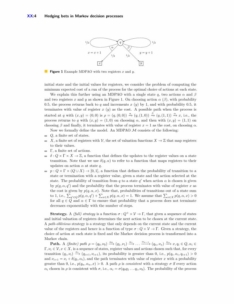
Figure 1 Example MDPAO with two registers x and y.

initial state and the initial values for registers, we consider the problem of computing theminimum expected cost of a run of the process for the optimal choice of actions at each state.

We explain this further using an MDPAO with a single state q, two actions α and β

and two registers x and y as shown in Figure 1. On choosing action α (β), with probability0.5, the process returns back to q and increments x (y) by 1, and with probability 0.5, itterminates with value of register x (y) as the cost. A possible path when the process isstarted at q with (x, y) = (0, 0) is ρ = (q, (0, 0)) α−→ (q, (1, 0)) β−→ (q, (1, 1)) α−→ x, i.e., theprocess returns to q with (x, y) = (1, 0) on choosing α, and then with (x, y) = (1, 1) onchoosing β and finally, it terminates with value of register x = 1 as the cost, on choosing α.

Now we formally define the model. An MDPAOM consists of the following:Q, a finite set of states.X, a finite set of registers with V , the set of valuation functions X → Z that map registersto their values.Γ, a finite set of actions.δ : Q× Γ×X → Z, a function that defines the updates to the register values on a statetransition. Note that we use δ(q, α) to refer to a function that maps registers to theirupdates on action α at state q.p : Q × Γ × (Q ∪X) → [0, 1], a function that defines the probability of transition to astate or termination with a register value, given a state and the action selected at thestate. The probability of transition from q to a state q′ when action α is chosen is givenby p(q, α, q′) and the probability that the process terminates with value of register x asthe cost is given by p(q, α, x). Note that, probabilities of transitions out of a state sumto 1, i.e.,

∑q′∈Q p(q, α, q′) +

∑x∈X p(q, α, x) = 1. We assume that

∑x∈X p(q, α, x) > 0

for all q ∈ Q and α ∈ Γ to ensure that probability that a process does not terminatedecreases exponentially with the number of steps.

Strategy. A (full) strategy is a function σ : Q+ ×V → Γ, that given a sequence of statesand initial valuation of registers determines the next action to be chosen at the current state.A path-oblivious strategy is a strategy that only depends on the current state and the currentvalue of the registers and hence is a function of type σ : Q× V → Γ. Given a strategy, thechoice of action at each state is fixed and the Markov decision process is transformed into aMarkov chain.

Path. A (finite) path ρ = (q0, ν0) α0−→ (q1, ν1) α1−→ . . .αn−1−−−→ (qn, νn) αn−−→ x, qi ∈ Q,αi ∈

Γ, νi ∈ V, x ∈ X, is a sequence of states, register values and actions chosen such that, for everytransition (qi, νi)

αi−→ (qi+1, νi+1), its probability is greater than 0, i.e., p(qi, αi, qi+1) > 0and νi+1 = νi + δ(qi, αi), and the path terminates with value of register x with a probabilitygreater than 0, i.e., p(qn, αn, x) > 0. A path ρ is consistent with a strategy σ if every actionαi chosen in ρ is consistent with σ, i.e., αi = σ(q0q1 . . . qi, ν0). The probability of the process


following the path ρ is given by Pr(ρ) = (∏n−1i=0 p(qi, αi, qi+1))p(qn, αn, x). The cost of the

path ρ is defined as f(ρ) = νn(x).Cost. Let Πσ(q, ν) be the set of all paths that start in q ∈ Q with register values ν and

are consistent with σ, i.e., Πσ(q, ν) = {ρ|(q0, ν0) = (q, ν), ρ is consistent with σ}. Given aninitial valuation of registers ν and a strategy σ, the expected cost of a run started from astate q is fσ(q, ν) =

∑ρ∈Πσ(q,ν) Pr(ρ) · f(ρ).

In the example shown in Figure 1, suppose the process starts with ν(x) = 0 and ν(y) = 0.For a strategy that always chooses α i.e. σ(qi, ν) = α, the process terminates after k steps withprobability 0.5k and cost k−1 and thus, the expected cost is (0×0.5+1×0.52+2×0.53+. . . ) =1. Similarly for a strategy that always chooses β, the expected cost is 1. Now for a strategythat alternately chooses α and β, i.e., σ(q2i, ν) = α and σ(q2i+1, ν) = β, we get a lowerexpected cost of 1

3 . In fact, this is the minimum expected cost. Note that, unlike traditionalMDPs, the optimal strategy chooses multiple actions at state q.

Problem. Given an MDPAO M, we consider here the problem of computing theminimum expected cost of a run ofM started in an initial state q ∈ Q with initial valuationof registers ν ∈ V. Let f(q, ν) denote this minimum expected cost and σ∗ the optimalstrategy, i.e., f(q, ν) = minσ fσ(q, ν), σ∗ = argminσfσ(q, ν).

Variations of the model. The above model can be further extended as follows. A firstextension is one where the update function δ depends also on the next state, along with thecurrent state and the action chosen. A second extension is one where, upon termination, thecost is a non-negative linear combination of register values rather than a single register’svalue. Note that our algorithms generalize to these extensions immediately and to keep thepresentation simple, we describe solutions only for the model defined above.

3 Useful results

We describe here some results that are useful in solving the problem of computing theminimum expected cost.

We first show that |fσ(q, ν)| is bounded by a linear function of maxx∈X |ν(x)| for allstrategies σ and thus, |f(q, ν)| is bounded by this function. We use this result to compute anapproximation for the minimum expected cost in Section 7 and to prove subsequent resultsin this section. Let pM be the maximum probability of continuation and δM be magnitudeof maximum change made to any register, in one step of the process. We state the result inthe following lemma.

I Lemma 1. Given ν ∈ V, for all q ∈ Q and strategies σ,

|fσ(q, ν)| ≤(

maxx∈X |ν(x)|1− pM

+ pMδM(1− pM )2

), B(max

x∈X|ν(x)|),

where pM = maxq∈Q,α∈Γ

(∑q′∈Q p(q, α, q′)

)and δM = maxq∈Q,α∈Γ,x∈X |δ(q, α, x)|.

Proof. We claim that for any strategy σ and for all i ≥ 0, the probability that the processdoes not terminate in first i steps, pi is bounded by piM , the absolute value of any register afteri steps, νi is bounded by (maxx∈X |ν(x)|+ iδM ) and thus, the absolute value of the expectedcost paid in the (i+ 1)th step by the process, ci, is bounded by piM (maxx∈X |ν(x)|+ iδM ).

We prove this by induction. It is trivially true when i = 0. Assuming it is true in the ithstep, we prove that it is also true in (i+ 1)th step. Probability that the process continues tothe next step at the (i+ 1)th step at any state and for any action chosen is less than pMand thus, pi+1 ≤ pipM = pi+1

M . Similarly, the register values can be changed by at most δM


in a step and thus, the absolute value of registers after (i+ 1) steps must be bounded bymaxx∈X |ν(x)|+ (i+ 1)δM . Note that the absolute value of expected cost paid at a state qwith register values ν′ for an action α is∣∣∑

x∈Γp(q, α, x)ν′(x)

∣∣ ≤ (maxx∈X|ν′(x)|

)∑x∈Γ

p(q, α, x) ≤ maxx∈X|ν′(x)|.

Therefore, ci+1 is bounded by the maximum probability to reach the (i+ 2)th step × theexpected cost paid in the (i+ 2)th step ≤ pi+1

M (maxx∈X |ν(x)|+ (i+ 1)δM ).Now, the absolute value of the total expected cost of strategy σ is less than

∑∞i=0 ci ≤∑∞

i=0(piM (maxx∈X |ν(x)|+ iδM )

). Since the probability of termination in each step is strictly

greater than 0, the maximum probability pM < 1 and the required result follows. J

Next, minimum expected cost f(q, ν) can be expressed recursively using the costs at thenext step, f(q′, ν + δ(q, α)). Let a cost function be a function Q× V → R that maps a stateand valuation of registers to a real valued cost and let the set of cost functions be C. Wedefine an operator T : C → C as follows.

Tg(q, ν) = minα∈Γ

(∑x∈X

p(q, α, x)ν(x) +∑q′∈Q

p(q, α, q′)g(q′, ν + δ(q, α)))

The minimum expected cost function f is a fixed point of this operator, i.e., Tf = f .In fact, we can show that a strategy σ is an optimal strategy if fσ is a fixed point of T , asstated in Lemma 2. Our proof for Lemma 2 closely follows the proof by Bertsekas et al in [4]to show that the recursive equation describing the stochastic shortest path problem has aunique solution which represents the optimal cost vector. We use this lemma to compute theoptimal strategies in Sections 5 and 6. Another consequence of this lemma is that we canlimit our investigation to path-oblivious strategies, i.e., strategies that only depend on thecurrent state and the current value of the registers.

I Lemma 2. Given a strategy σ in an MDPAOM, the cost function fσ is a fixed point ofT , i.e., Tfσ(q, ν) = fσ(q, ν) for all q ∈ Q and ν ∈ V, if and only if σ is an optimal strategyand fσ is the minimum expected cost function.

Proof. To prove this lemma, we show that set of the cost functions, realizable by strategies,forms a partially ordered set such that the operator T has a unique fixed point in this set.Since the minimum expected cost function must be the least fixed point of T , any fixed pointof T is the required minimum expected cost function.

For a strategy σ, we define a new operator on cost functions, Tσ : C → C, where Tσgcomputes the cost of using strategy σ for one step and then paying the cost as given by g.Let α = σ(q, ν), we have:

Tσg(q, ν) =∑x∈X

p(q, α, x)ν(x) +∑q′∈Q

p(q, α, q′)g(q′, ν + δ(q, α))

We also define a complete partial order L on cost functions as follows. Let f>, f⊥ ∈C be the two cost functions defined by f>(q, ν) = B(maxx∈X |ν(x)|) and f⊥(q, ν) =−B(maxx∈X |ν(x)|), where B is defined in Lemma 1. Further, g ≤ h, where g, h ∈ C,if for all q ∈ Q, ν ∈ V , g(q, ν) ≤ h(q, ν). Now, L is a complete partial order for relation ≤ onthe set {g ∈ C | f⊥ ≤ g ≤ f>}. Note that by Lemma 1, for all strategies σ, f⊥ ≤ fσ ≤ f>and hence fσ ∈ L.

The operators T and Tσ are closed in L, i.e. g ∈ L ⇒ Tg, Tσg ∈ L since Tf> ≤f>, Tσf> ≤ f> and Tf⊥ ≥ f⊥, Tσf⊥ ≥ f⊥ (by Lemma 1). Further, operators T and Tσ


are monotonic and continuous, since they apply linear transformations and the minimumoperator on cost functions, which preserve both properties. Hence, by Kleene’s fixed pointtheorem, both T and Tσ must have a least fixed point in L given by limk→∞ T kf⊥ andlimk→∞ T kσ f⊥ respectively.

Next, we prove that Tσ has a unique fixed point in L. To prove this, we show thatfor all g, h ∈ L, limk→∞ T kσ g(q, ν) = limk→∞ T kσh(q, ν). Note that, T kσ g corresponds to theexpected cost of using strategy σ for first k steps and then terminating with the cost givenby g at the (k + 1)th step. Hence, the difference T kσ g(q, ν)− T kσh(q, ν) corresponds to thedifference in costs paid at the (k + 1)th step, since the cost paid till k steps is same forboth T kσ g(q, ν) and T kσh(q, ν). As described in the proof for Lemma 1, the probability ofthe process not terminating in first k steps is bounded by pkM and the magnitude of registervalues are bounded by (maxx∈X |ν(x)|+ kδM ). Since g, h ∈ L, we have:

|T kσ g(q, ν)− T kσh(q, ν)| ≤ 2pkMB(

maxx∈X|ν(x)|+ kδM

).

Note that pkM decreases exponentially with k, whereas B(maxx∈X |ν(x)|+ kδM ) increasesonly linearly with k. Hence, limk→∞(T kσ g(q, ν)− T kσh(q, ν)) = 0, and thus Tσ has a uniquefixed point in L.

Now we prove that T has a unique fixed point in L. Suppose T had two fixed points inL, say f1, f2. Then we can find strategies σ1, σ2 such that Tσ1f1 = f1 and Tσ2f2 = f2 byusing the actions that minimize Tf1 and Tf2 respectively. Further, Tf1 ≤ Tσ2f1 since Tf1corresponds to the minimum of the costs for different actions, while Tσ2f1 corresponds toone of these costs. This implies f1 = limk→∞ T kf1 ≤ limk→∞ T kσ2

f1 = f2 and thus, f1 ≤ f2.By a symmetric argument, f2 ≤ f1. Hence, T must have a unique fixed point in L. Theminimum expected cost f is the least fixed point of T in L and hence, any fixed point of Tin L is the required minimum expected cost. J

Our final result shows that the optimal strategy σ∗ depends only on the relative differencebetween the initial register values and not their absolute values. We state it in Lemma 3.We prove this by showing that f(q, ν + k)− k is also a fixed point of T and hence, must beequal to f(q, ν). Note that, this result can be used to reduce a model with |X| registers intoa model with |X| − 1 registers. We use it to simplify the problem in Section 6.

I Lemma 3. Given an MDPAOM, for all q ∈ Q, ν ∈ V, k ∈ Z, it holds that f(q, ν + k) =f(q, ν) + k, where (ν + k)(x) = ν(x) + k for all x ∈ X.

Proof. We use Lemma 2 to prove this. Let g ∈ C be a function such that g(q, ν) =f(q, ν + k)− k for all q ∈ Q and ν ∈ V . Note that g may not lie in the complete partial orderL as described in the proof for Lemma 2. However if we define the partial order L′ usingf ′> = f>+ |k|(1+ 1

1−pM ) and f ′⊥ = f⊥−|k|(1+ 11−pM ), the proof of Lemma 2 still follows and

T must have a unique fixed point in L′. Also g belongs to L′ since |g(q, ν)| ≤ |f(q, ν+k)|+ |k|.Further,

Tg(q, ν) = T (f(q, ν + k)− k)= Tf(q, ν + k)− k= f(q, ν + k)− k= g(q, ν).

Hence, g is a fixed point of T and thus, by Lemma 2, it must be the minimum expected costfunction f . J


4 Markov chains with alternative objectives

We consider a special case of the problem when the set of actions consists of a single action,i.e. Γ = {α}. Since f is a fixed point for the operator T as defined in Section 3, for all q ∈ Qand ν ∈ V,

f(q, ν) =∑x∈X

p(q, x)ν(x) +∑q′∈Q

p(q, q′)f(q′, ν + δ(q)). (1)

The above system of equations may have more than one solutions. However, we showthat f(q, ν) is a linear function of the initial register values ν for all q ∈ Q, as stated inLemma 4. The cost incurred by a path ρ consists of two components: the initial value of aregister x, ν(x) and the updates to x along the path which are independent of ν. Also, thecontribution of ν(x) to the expected cost f(q, ν) depends only on the probability with whichpaths starting at (q, ν) end in x, which again is independent of ν. Therefore, f(q, ν) must belinear in ν.

I Lemma 4. Given an MDPAO with a single action, the minimum expected cost f(q, ν) islinear in ν, i.e., for all q ∈ Q and ν ∈ V, it holds that f(q, ν) =

∑x∈X aq,xν(x) + f(q, ν0),

where ν0(x) = 0 for all x ∈ X and aq,x is the probability that a path starting at (q, ν) ends inregister x.

Proof. To prove the lemma we show that f(q, ν + δx) = f(q, ν) + aq,xd, where δx(x) = d

and δx(y) = 0 for all y ∈ X \ {x}, for some d ∈ Z. Let ρ = (q0, ν0) α0−→ (q1, ν1) α1−→ . . .αn−1−−−→

(qn, νn) αn−−→ y and ρ′ = (q0, ν′0) α0−→ (q1, ν

′1) α1−→ . . .

αn−1−−−→ (qn, ν′n) αn−−→ y be paths that followthe same sequence of states but are started with different valuations of registers ν and ν + δxrespectively. We can see that ν′i = νi + δx for all i, since the same changes are made toboth ν and ν′ along the way. Therefore, if a path ρ′ terminates in x, denoted by ρ′ x,then f(ρ′) = ν′n(x) = νn(x) + d = f(ρ) + d, and f(ρ′) = f(ρ) otherwise. Also note thatPr(ρ′) = Pr(ρ).

By definition, f(q, ν + δx) =∑ρ′∈Π(q,ν+δx)(Pr(ρ′)f(ρ′)). Since f(ρ′) = f(ρ) + d for all

runs ρ′ x, f(q, ν + δx) = f(q, ν) + d∑ρ∈Π(q,ν),ρ x Pr(ρ) which implies f(q, ν + δx) =

f(q, ν) + aq,xd. The required lemma follows immediately. J

Now, from (1) and Lemma 4, we can compute f(q, ν) by solving the following system oflinear equations.

aq,x = p(q, x) +∑q′∈Q

p(q, q′)aq′,x

f(q, ν0) =∑q′∈Q

p(q, q′)(∑x∈X

aq′,xδ(q, x) + f(q′, ν0))

The above system consists of |Q| × (|X|+ 1) equations and variables and thus, can be solvedin O(|Q|3|X|3) time using a linear constraint solver.

I Theorem 5. The problem of computing f(q, ν) for q ∈ Q and ν ∈ V for an MDPAOMwith a single action can be solved in O(|Q|3|X|3) time.


5 Two action single state MDPs with alternative objectives

In this section, we solve the problem for an MDPAO M where Q = {q} and Γ = {α, β}.To simplify notation, let ax = p(q, α, x), bx = p(q, β, x), a0 = p(q, α, q) and b0 = p(q, β, q).Further, let the register updates be δα = δ(q, α) and δβ = δ(q, β).

We observe that in this case while the minimum expected cost f(ν) is no longer a linearfunction of ν, the choice of optimal action in the optimal strategy does depend on a linearpreference function P of current register values. So if P (ν) ≤ 0 then the optimal action at νis α i.e. σ∗(ν) = α, and otherwise σ∗(ν) = β.

To define P , we need to consider the change in preference ∆P on taking actions α andβ. Since P (ν) is a linear function of ν, the change in preference ∆P (δ) = P (ν + δ)− P (ν)depends only on the change in register values δ. We define ∆P (δ) as follows:

∆P (δ) =∑x∈X

(ax

1− a0− bx

1− b0

)δ(x).

Now ∆P (δα) and ∆P (δβ) capture the change in preference on taking the two actions, whereδα and δβ are the corresponding register updates. Depending on whether these values arepositive or negative, we can have four possible scenarios.

To illustrate this further, consider the example shown in Figure 1 which is also an instanceof this model. On choosing α, the process either terminates with value of register x orincrements x and returns to q. Note that if the process does not terminate, the value of xincreases and we are likely to pay a higher cost by choosing α in the next step. Hence, ourpreference P to choose β increases. Similarly on choosing β, our preference P to choose βdecreases. This corresponds to the case where ∆P (δα) ≥ 0 and ∆P (δβ) < 0 and the optimalstrategy oscillates between choosing the two actions.

Now we give a concrete definition of the preference function P for the different scenariosdescribed above. Let fw(ν) be the cost of an infinite sequence of actions given by an infiniteword w = w1w2w3 . . . in {α, β}ω. Note that fαw(ν) =

∑x∈X axν(x) + a0fw(ν + δα) and

fβw(ν) =∑x∈X bxν(x) + b0fw(ν + δβ). We can also compute fαω(ν) by reducingM to a

Markov chain where action α is chosen always, and fαω(ν) =∑x∈X

(axν(x)1−a0

+ a0axδα(x)(1−a0)2

).

Using this, we can further compute fβαω (ν). We can compute fβω (ν) and fαβω (ν) similarly.Further, for all infinite words w, the difference fαβw(ν)−fβαw(ν) =

∑x∈X(((1− b0)ax− (1−

a0)bx)ν(x) + a0bxδα(x)− b0axδβ(x)) and is independent of w. We abbreviate this differenceas fαβ·(ν)− fβα·(ν). We use these quantities to define P (ν) and the optimal strategy σ∗ inLemma 6.

I Lemma 6. In a two action single state MDPAOM, if P (ν) ≤ 0, then the optimal strategyat ν, σ∗(ν) = α and otherwise σ∗(ν) = β, where P (ν) is defined as follows:1. If ∆P (δα) ≥ 0 and ∆P (δβ) < 0, P (ν) = fαβ·(ν)− fβα·(ν).2. If ∆P (δα) ≥ 0 and ∆P (δβ) ≥ 0, P (ν) = fαβω (ν)− fβω (ν).3. If ∆P (δα) < 0 and ∆P (δβ) < 0, P (ν) = fαω (ν)− fβαω (ν).4. If ∆P (δα) < 0 and ∆P (δβ) ≥ 0, P (ν) = fαω (ν)− fβω (ν).

Proof. To prove this lemma, we show that in each case, fσ∗ is a fixed point of T and thenby Lemma 2, σ∗ is the optimal strategy. To compute the optimal action at ν, we need toconsider the difference between the minimum expected cost on choosing action α and thaton choosing β. This would require us to consider all possible sequences of actions startingfrom α and β and compute the expected cost for each sequence, which would be difficult.However, Lemma 2 helps us break down the problem into recursive cases, and consider only


a few of sequences of actions for both α and β and whichever leads to a lower cost gives thedesired optimal action. For Cases 1, 2 and 3, we also give alternate proofs, since fσ∗ is onlyrecursively defined in these cases and a closed form representation is not available.

Case 4 : ∆P (δα) < 0,∆P (δβ) ≥ 0, P (ν) = fαω(ν) − fβω(ν). It is easy to see thatfσ∗(ν) = min(fαω (ν), fβω(ν)). This is because, if α is preferred in the current state at ν, it isalso preferred in all subsequent steps and thus, αω should lead to the minimum expectedcost. Similarly, for β. We need to show that Tfσ∗(ν) = fσ∗(ν) for all ν ∈ V. SupposeP (ν) ≤ 0. Then, P (ν + δα) ≤ 0 since ∆P (δα) < 0 and thus, fσ∗(ν + δα) = fαω(ν + δα).Therefore, the cost of taking action α at ν is cα = fαω(ν). If P (ν + δβ) > 0, then the costof taking action β, at ν is cβ = fβω(ν) and therefore, Tfσ∗(ν) = min(cα, cβ) = fσ∗(ν). IfP (ν + δβ) < 0, then cβ = fβαω(ν). But we can show that fαω(ν) − fβαω(ν) = fαω(ν) −fβω(ν) − (fβαω(ν) − fβω(ν)) = P (ν) − b0P (ν + δβ) = (1 − b0)P (ν) − b0∆P (δβ) ≤ 0. Thisimplies fαω(ν) ≤ fβαω(ν) and therefore, Tfσ∗(ν) = fσ∗(ν). The other case, P (ν) > 0 issymmetric and thus, σ∗ is the optimal strategy.

Case 1 : ∆P (δα) ≥ 0,∆P (δβ) < 0, P (ν) = fαβ·(ν) − fβα·(ν). Note that the optimalstrategy σ∗ here oscillates between α and β. Thus, the cost fσ∗ can be defined only recursivelyand its exact representation can not be known a priori. Therefore, we use the recursivedefinition to show that it is the fixed point. We also give an alternate proof based on anexchange argument for clarity.

We define fσ∗(ν) as follows. If P (ν) ≤ 0, fσ∗(ν) = fασ∗(ν) =∑x∈X axν(x)+a0fσ∗(ν+δα)

else, fσ∗(ν) = fβσ∗(ν). We also assume that fσ∗(ν) is the minimum expected cost i.e.fσ∗(ν) ≤ fw(ν) for all w ∈ {α, β}ω and ν ∈ V. Now we show that Tfσ∗ = fσ∗ . SupposeP (ν) ≤ 0. Then since ∆P (δβ) < 0, P (ν + δβ) < 0 and fσ∗(ν + δβ) = fασ∗(ν + δβ) or α isthe preferred action at ν + δβ . Thus on taking action β at ν, the cost is cβ = fβασ∗(ν).Since P (ν) ≤ 0, fαβσ∗(ν) ≤ fβασ∗(ν) and thus, fαβσ∗(ν) ≤ cβ . Further by assumption, cα =fασ∗(ν) is the minimum expected cost of taking action α at ν and thus, cα ≤ fαβσ∗(ν) ≤ cβ .Hence Tfσ∗(ν) = min{cα, cβ} = fασ∗(ν) = fσ∗(ν). Further by assumption cα and cβ arethe minimum expected costs of taking actions α and β and thus Tfσ∗(ν) is the minimumexpected cost for all ν. The sub-case when P (ν) > 0 is symmetric and thus, σ∗ is the optimalstrategy.

Alternate proof. We now show a proof based on an exchange argument. SupposeP (ν) ≤ 0. We can show that every infinite sequence of actions at ν can be transformed to asequence starting with action α with a lower expected cost, by exchanging pairs βα withαβ. Formally, we show that for all infinite sequence of actions βw,, there exists w′ suchthat fαw′(ν) ≤ fβw(ν). First, we can show by induction on k that for all k > 0, z ∈ {α, β}ω,fαβkz(ν) ≤ fβkαz(ν). Base case is implied by P (ν) ≤ 0. Assuming it is true for k − 1, weshow that it holds for k. Since ∆P (δβ) ≤ 0, we can see that P (ν + (k − 1)δβ) ≤ 0 andthus, fβk−1αβz(ν) ≤ fβkαz(ν). Further, by inductive hypothesis fαβk−1z(ν) ≤ fβk−1αz(ν) forall z and thus, fαβkz(ν) ≤ fβkαz(ν). Further, we can show that fαβω(ν) ≤ fβω(ν) because,fαβω (ν)− fβω (ν) =

∑∞i=0 b

i0P (ν+ iδβ) ≤ 0. Hence, for infinite sequence of actions, βw, there

is a sequence starting with α that has a lower cost and thus, α must be the optimal actionat ν. Similarly, we can show that when P (ν) > 0, σ∗(ν) = β.

Case 2 : ∆P (δα) ≥ 0,∆P (δβ) ≥ 0, P (ν) = fαβω(ν)− fβω(ν). We again give two proofs,one based on fixed point and other based on an exchange argument like in Case 1.

We define fσ∗(ν) as follows. If P (ν) > 0, fσ∗(ν) = fβω(ν) else fσ∗(ν) = fασ∗(ν). Also,like in Case 1, we assume that fσ∗(ν) is the minimum expected cost i.e. fσ∗(ν) ≤ fw(ν)for all w ∈ {α, β}ω and ν ∈ V. We show that Tfσ∗ = fσ∗ . Suppose P (ν) ≥ 0. ThenP (ν + δβ) ≥ 0, P (ν + δα) ≥ 0, and cα = fαβω(ν), cβ = fβω(ν). Since P (ν) ≥ 0, cα ≥ cβ


q, .75

y = y + 1

q, .50

y = y + 1

q, .25

y = y + 1

q, 0

x = x+ 1

y y y x

1/2

1/2

1/2

1/2

1/2

1/21/2

1/2

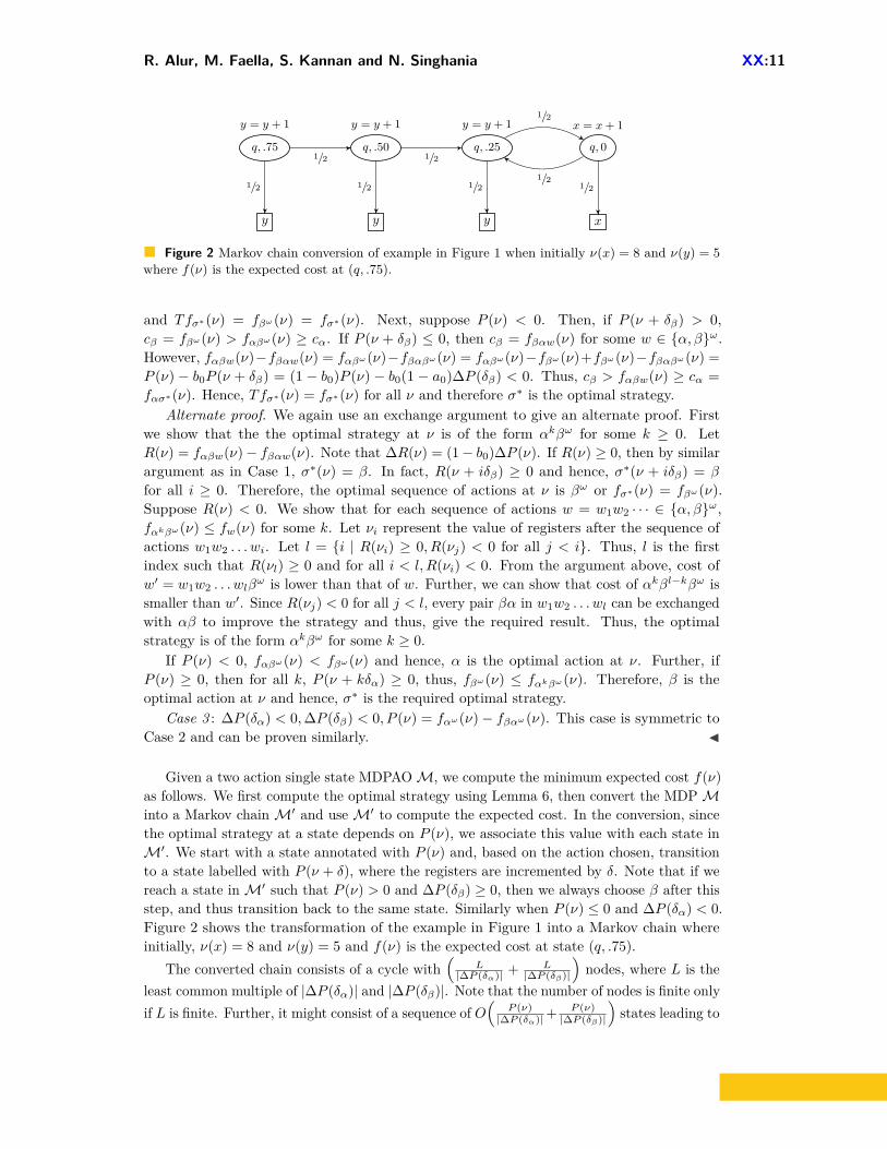
Figure 2 Markov chain conversion of example in Figure 1 when initially ν(x) = 8 and ν(y) = 5where f(ν) is the expected cost at (q, .75).

and Tfσ∗(ν) = fβω(ν) = fσ∗(ν). Next, suppose P (ν) < 0. Then, if P (ν + δβ) > 0,cβ = fβω(ν) > fαβω(ν) ≥ cα. If P (ν + δβ) ≤ 0, then cβ = fβαw(ν) for some w ∈ {α, β}ω.However, fαβw(ν)−fβαw(ν) = fαβω (ν)−fβαβω (ν) = fαβω (ν)−fβω (ν)+fβω (ν)−fβαβω (ν) =P (ν) − b0P (ν + δβ) = (1 − b0)P (ν) − b0(1 − a0)∆P (δβ) < 0. Thus, cβ > fαβw(ν) ≥ cα =fασ∗(ν). Hence, Tfσ∗(ν) = fσ∗(ν) for all ν and therefore σ∗ is the optimal strategy.

Alternate proof. We again use an exchange argument to give an alternate proof. Firstwe show that the the optimal strategy at ν is of the form αkβω for some k ≥ 0. LetR(ν) = fαβw(ν)− fβαw(ν). Note that ∆R(ν) = (1− b0)∆P (ν). If R(ν) ≥ 0, then by similarargument as in Case 1, σ∗(ν) = β. In fact, R(ν + iδβ) ≥ 0 and hence, σ∗(ν + iδβ) = β

for all i ≥ 0. Therefore, the optimal sequence of actions at ν is βω or fσ∗(ν) = fβω(ν).Suppose R(ν) < 0. We show that for each sequence of actions w = w1w2 · · · ∈ {α, β}ω,fαkβω(ν) ≤ fw(ν) for some k. Let νi represent the value of registers after the sequence ofactions w1w2 . . . wi. Let l = {i | R(νi) ≥ 0, R(νj) < 0 for all j < i}. Thus, l is the firstindex such that R(νl) ≥ 0 and for all i < l,R(νi) < 0. From the argument above, cost ofw′ = w1w2 . . . wlβ

ω is lower than that of w. Further, we can show that cost of αkβl−kβω issmaller than w′. Since R(νj) < 0 for all j < l, every pair βα in w1w2 . . . wl can be exchangedwith αβ to improve the strategy and thus, give the required result. Thus, the optimalstrategy is of the form αkβω for some k ≥ 0.

If P (ν) < 0, fαβω(ν) < fβω(ν) and hence, α is the optimal action at ν. Further, ifP (ν) ≥ 0, then for all k, P (ν + kδα) ≥ 0, thus, fβω(ν) ≤ fαkβω(ν). Therefore, β is theoptimal action at ν and hence, σ∗ is the required optimal strategy.

Case 3 : ∆P (δα) < 0,∆P (δβ) < 0, P (ν) = fαω(ν)− fβαω(ν). This case is symmetric toCase 2 and can be proven similarly. J

Given a two action single state MDPAOM, we compute the minimum expected cost f(ν)as follows. We first compute the optimal strategy using Lemma 6, then convert the MDPMinto a Markov chainM′ and useM′ to compute the expected cost. In the conversion, sincethe optimal strategy at a state depends on P (ν), we associate this value with each state inM′. We start with a state annotated with P (ν) and, based on the action chosen, transitionto a state labelled with P (ν + δ), where the registers are incremented by δ. Note that if wereach a state inM′ such that P (ν) > 0 and ∆P (δβ) ≥ 0, then we always choose β after thisstep, and thus transition back to the same state. Similarly when P (ν) ≤ 0 and ∆P (δα) < 0.Figure 2 shows the transformation of the example in Figure 1 into a Markov chain whereinitially, ν(x) = 8 and ν(y) = 5 and f(ν) is the expected cost at state (q, .75).

The converted chain consists of a cycle with(

L|∆P (δα)| + L

|∆P (δβ)|

)nodes, where L is the

least common multiple of |∆P (δα)| and |∆P (δβ)|. Note that the number of nodes is finite onlyif L is finite. Further, it might consist of a sequence of O

(P (ν)|∆P (δα)|+

P (ν)|∆P (δβ)|

)states leading to


MDPAO OC-MDP p1CA

2-register

minimumexpectedcost

minimum ex-pected accumu-lated reward

++

tie-less

eventuallycounter-oblivious opti-mal strategy

expected accu-mulated reward

Sec. 6.1

Sec. 6.2 Sec. 6.3

Figure 3 Diagram of the reductions between different models developed in Section 6.

the cycle. Thus, time to compute cost function in the cycle is O((

L|∆P (δα)| + L

|∆P (δβ)|

)3|X|3

)and f(ν) can be computed in O

((P (ν)|∆P (δα)| + P (ν)

|∆P (δβ)|

)|X|)time using the costs in the cycle.

I Theorem 7. The problem of computing f(q, ν) for a two action single state MDPAOM,i.e., Γ = {α, β} and Q = {q}, can be solved in time

O( ( L

|∆P (δα)| + L

|∆P (δβ)|

)3|X|3 +

( P (ν)|∆P (δα)| + P (ν)

|∆P (δβ)|

)|X|),

where L is the l.c.m. of |∆P (δα)| and |∆P (δβ)|. Note that if |∆P (δα)|/|∆P (δβ)| is irrational,then L is infinite.

6 Two register MDPs with alternative objectives

In this section, we tackle the problem for MDPAOs with two registers x, y, and an arbitrarynumber of states and actions. Note that by Lemma 3, the optimal strategy depends onlyon the relative difference between the registers and the strategy needs to maintain a singlecounter that keeps track of the difference between the values of the two registers.

We show the following results in this section. First, we reduce our problem to theminimum expected accumulated reward problem for one-counter MDPs (OC-MDPs), whichis another decision problem whose decidability status is open. Next, we show that for theclass of tie-less MDPAOs, the optimal strategy is eventually counter-oblivious, i.e., thereexists a natural number k such that in each state the strategy plays in the same way for allvalues of the counter higher than k. In turn, this property implies decidability by a reductionof the corresponding OC-MDP to the expected accumulated reward problem for probabilistic1-counter automata (p1CAs). This sequence of results is summarized in Figure 3.

6.1 Reduction to one-counter Markov decision processesThe problem of computing the minimum expected cost of a 2-register MDPAO can be easilyreduced to the minimum expected accumulated reward problem for one-counter Markovdecision processes (OC-MDPs) [6, 5]. We employ OC-MDPs with boundary, which meansthat the counter value is always non-negative.

A one-counter MDP is a tuple A = (S,Γ,∆0,∆>0) 1, where S is a finite set of controlstates, Γ is a finite set of actions, and ∆0, ∆>0 are the transitions, with the intended meaning

1 For technical convenience, our presentation of OC-MDPs includes explicit actions and rewards attachedto transitions. It is straightforward to convert this form to the one of Brádzil et al. [6, 8], where rewardsare represented by a simple reward function.


that ∆0 applies when the counter is zero and ∆>0 applies otherwise. Each transition is atuple of the type:

(source, action, probability, counter update, reward, destination).

So, we have ∆0 ⊆ S×Γ×[0, 1]×{0, 1}×Q+×S and ∆>0 ⊆ S×Γ×[0, 1]×{−1, 0, 1}×Q+×S.Moreover, for all s ∈ S and γ ∈ Γ, the sum of the probabilities of all transitions in ∆0 (resp.,∆>0) starting from s and γ is 1. A transition (s, α, p, d, r, s′) ∈ δ>0 signifies that when thesystem is in control state s with a positive value of its counter, action α may lead to state s′with probability p, while updating the counter value from n to n+ d and obtaining reward r.

The reward associated with a finite run is the sum of the rewards of each transition. Theminimum expected accumulated reward problem takes as inputs an OC-MDP, two controlstates s, s′, and an initial counter value n, and consists of computing the minimum over allpolicies of the expected reward along all runs that start in (s, n) and end in (s′, 0). As usual,by “computing a value” we mean decide whether such value is smaller than or equal to agiven rational number.

Consider a 2-register MDPAOM with non-negative register updates. In order to convertit into an OC-MDP, we first restrict the register updates to the values {0, 1}. This can beeasily accomplished by adding more states and splitting a transition with updates (+dx,+dy)into a sequence of max{dx, dy} transitions with {0, 1} updates. Notice that the newlyadded transitions violate the assumption that each transition carries a positive probabilityof termination. However, in the resulting system each sequence of k transitions carries apositive probability of termination, for a bounded k. Hence, the only consequence is a slightmodification to the bound provided by Lemma 1.

Once register updates have been simplified, the reduction is based on the following idea.Let f(q, x, y) represent the minimum expected cost when the initial state is q and initialvalues of registers are given by x and y. By Lemma 3, we know that

f(q, x, y) = f(q, x− y, 0) + y = f(q, 0, y − x) + x. (2)

Clearly, at least one of x− y and y − x is non-negative. By (2), to compute the minimumexpected cost of an arbitrary configuration (q, x, y) it is sufficient to know the minimumexpected cost of all configurations of the type (q, z, 0) and (q, 0, z) for all z ≥ 0. All theseconfigurations can be encoded by an OC-MDP, whose counter encodes z and whose controlstates are pairs (q, r), where r ∈ {x, y} identifies which register has value z. An equivalentway to look at this encoding is that the counter stores the difference between the registerthat currently holds the highest value and the other register, and the flag r encodes which ofthe two registers holds the highest value.

It remains to encode the cost structure of the MDPAO. To this purpose, suppose thatwe are in the configuration (q, z, 0), for some z ≥ 0 (encoded by the OC-MDP state (q, x)with counter value z), and we want to simulate the effect of an action γ, which leads to stateq′ with probability p(q, γ, q′) and carries register updates δ(q, γ, x) = dx and δ(q, γ, y) = dy.Then, Lemma 3 tells us that f(q′, z + dx, dy) = f(q′, z + dx − dy, 0) + dy. So, assuming thatz + dx − dy ≥ 0, the corresponding OC-MDP will move with probability p(q, γ, q′) fromstate (q, x) to state (q′, x), while updating the counter from z to z + dx − dy, and gaining animmediate reward of dy. Two special states called accrue and stop model the termination ofthe MDPAO. We restrict the analysis to non-negative register updates so that the rewardsin the OC-MDP will be non-negative too.

Formally, given a 2-register MDPAO M, we define the corresponding OC-MDP A asfollows. The set of control states S comprises pairs (q, r), where q ∈ Q and r ∈ {x, y},


plus the special states accrue and stop. The actions are the same as in the MDPAO. Forall q, q′ ∈ Q, r ∈ {x, y}, and γ ∈ Γ, the following transitions belong to ∆0 (recall thatδ(·, ·, ·) ∈ {0, 1}):

((q, r), γ, p(q, γ, q′), δ(q, γ, x)− δ(q, γ, y), δ(q, γ, y), (q′, x)) whenever δ(q, γ, x) ≥ δ(q, γ, y)

((q, r), γ, p(q, γ, q′), δ(q, γ, y)− δ(q, γ, x), δ(q, γ, x), (q′, y)) whenever δ(q, γ, x) < δ(q, γ, y)

(accrue, γ, 1, 0, 0, stop)

Similarly, the following transitions belong to ∆>0:

((q, x), γ, p(q, γ, q′), δ(q, γ, x)− δ(q, γ, y), δ(q, γ, y), (q′, x))((q, y), γ, p(q, γ, q′), δ(q, γ, y)− δ(q, γ, x), δ(q, γ, x), (q′, y))(accrue, γ, 1,−1, 1, accrue)(stop, γ, 1,−1, 0, stop)

Moreover, both in ∆0 and in ∆>0 we find the following transitions, where ¬r denotes theregister different from r:

((q, r), γ, p(q, γ, r), 0, 0, accrue) ((q, r), γ, p(q, γ,¬r), 0, 0, stop)

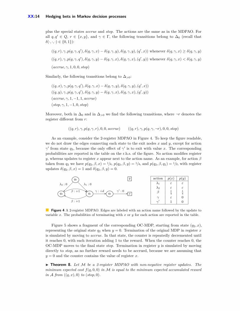
As an example, consider the 2-register MDPAO in Figure 4. To keep the figure readable,we do not draw the edges connecting each state to the exit nodes x and y, except for actionγ′ from state q3, because the only effect of γ′ is to exit with value x. The correspondingprobabilities are reported in the table on the r.h.s. of the figure. No action modifies registery, whereas updates to register x appear next to the action name. As an example, for action βtaken from q2 we have p(q2, β, x) = 1/4, p(q2, β, y) = 1/4, and p(q2, β, q1) = 1/2, with registerupdates δ(q2, β, x) = 1 and δ(q2, β, y) = 0.

q0

q1q2 q3 x

y

λ1 : 0λ2 : 0

β : +1

γ : +dβ : +1 γ′ : 0

action p(x) p(y)λ1 ε ε

λ2 ε ε

β 14

14

γ ε 0γ′ 1 0

Figure 4 A 2-register MDPAO. Edges are labeled with an action name followed by the update tovariable x. The probabilities of terminating with x or y for each action are reported in the table.

Figure 5 shows a fragment of the corresponding OC-MDP, starting from state (q2, x),representing the original state q2 when y = 0. Termination of the original MDP in register xis simulated by moving to accrue. In that state, the counter is repeatedly decremented untilit reaches 0, with each iteration adding 1 to the reward. When the counter reaches 0, theOC-MDP moves to the final state stop. Termination in register y is simulated by movingdirectly to stop, as no further reward needs to be accrued, because we are assuming thaty = 0 and the counter contains the value of register x.

I Theorem 8. Let M be a 2-register MDPAO with non-negative register updates. Theminimum expected cost f(q, 0, 0) inM is equal to the minimum expected accumulated rewardin A from ((q, x), 0) to (stop, 0).


q2, x

accrue stop

q1, x∆∗ : β, 1

2 , 1, 0

∆∗ : β, 14 , 0, 0 ∆∗ : β, 1

4 , 0, 0

∆>0 : ∗, 1,−1, 1

∆0 : ∗, 1, 0, 0

∆>0 : ∗, 1,−1, 0

Figure 5 A fragment of the OC-MDP corresponding to the MDPAO in Figure 4. Edges reportaction, probability, counter update, and reward. The asterisk is used as a wildcard.

The minimum expected accumulated reward problem is a generalization of the minimumexpected termination time problem considered in [8]. Neither problem is known to bedecidable for OC-MDPs, whereas both are solvable in PSPACE for probabilistic 1-counterautomata (p1CAs) [9, 7], which are equivalent to OC-MDPs with a single action. InSubsection 6.3, we employ the decidability on p1CAs to solve the minimum expected costproblem on a class of 2-register MDPAOs.

6.2 Tie-less MDPAOsIn this subsection, we introduce the class of tie-less MDPAOs and show that for this classthere exists an optimal strategy that is eventually counter-oblivious.

Note that from equation (2), f(q, x, y) can be computed from f(q, x− y, 0) and thus itsuffices to compute f(q, n, 0), with n ∈ Z. In the following we write f(q, n) as a shortcut forf(q, n, 0). A simple strategy is a function σ : Q→ Γ and we denote by S the set of all simplestrategies. An ω-strategy is an infinite sequence of simple strategies, i.e., an element of Sω.Notice that given a full strategy σ, an initial state q and an initial valuation ν there existsat least one ω-strategy π that is equivalent to it. In particular, it holds fσ(q, ν) = fπ(q, ν).Hence, in order to compute f(q, 0, 0) it is sufficient to consider ω-strategies rather than fullstrategies.

Similarly to Lemma 4, we can show that for all ω-strategies π, fπ(q, n) is a linear functionof n, i.e.: fπ(q, n) = slopeq,x(π) · n + fπ(q, 0), where slopeq,x(π) is the probability that apath starting at q ends in register x under strategy π. Notice that slopeq,x(π) generalizesthe notation aq,x used in Section 4 to denote the probability of terminating with a specificregister.

In fact, if the same simple strategy σ ∈ S is used at every step (equivalently, the ω-strategyσω is used), the system becomes equivalent to an MDPAO with a single action and thereforeslopeq,x(σω) can be computed for all q in polynomial time as explained in Section 4. Inparticular, the simple strategy α with the minimum x-slope can be found by solving thefollowing linear program, on the set of variables {aq | q ∈ Q}.

maximize:∑q∈Q

aq (3)

subject to: aq ≤ p(q, γ, x) +∑q′∈Q

p(q, γ, q′)aq′ ∀ q ∈ Q, γ ∈ Γ

The optimal solution a∗ provides the minimal x-slope in each state. We say that theMDPAO is x-tie-less if there exists a unique simple strategy α that has the minimum x-slopefrom all states q. Equivalently, the MDPAO is x-tie-less if at a∗ exactly one of the constraints


for each state is tight, i.e., for all q there exists a unique αq ∈ Γ such that

a∗q = p(q, αq, x) +∑q′∈Q

p(q, αq, q′)a∗q′ . (4)

We can similarly define the y-slope of a strategy as the probability of terminating inregister y using that strategy. Since runs terminate with probability one, for each strategythe sum of the x-slope and the y-slope is 1. We then say that the MDPAO is y-tie-less ifthere exists a unique simple strategy that has the minimum y-slope (or equivalently themaximum x-slope) from all states. Finally, the MDPAO is tie-less if it is both x-tie-less andy-tie-less.

Notice that if an MDPAO is not tie-less then it can be made tie-less by an arbitrarilysmall perturbation of its transition probabilities. In contrast, a tie-less MDPAO can beperturbed by a sufficiently small amount and still be tie-less. So, being tie-less is a robustproperty of MDPAOs, whereas its opposite is not. In the following Lemmas 9-12 we assumethat the MDPAO is x-tie-less and α is the simple strategy with minimum x-slope from allstates.

By inspecting the linear program (3), we observe that, for all q ∈ Q, the slope of using αindefinitely cannot be improved (i.e., lowered) by starting with any other action. This isformalized by the following result.

I Lemma 9. For all σ ∈ S and q ∈ Q, we have that slopeq,x(σαω) ≥ slopeq,x(αω).

The following lemma extends the previous one from simple strategies to arbitrary ω-strategies.

I Lemma 10. For all π ∈ Sω and q ∈ Q, we have that slopeq,x(π) ≥ slopeq,x(αω).

Proof. First, we prove the result for an ω-strategy that starts with an arbitrary finite prefixand then switches permanently to α, i.e., a strategy of the form π = ταω, for τ ∈ S∗. Weproceed by induction on |τ |. If |τ | = 0, the result is trivial. Otherwise, τ = τ0τ

′ and theinduction hypothesis guarantees that slopeq,x(τ ′αω) ≥ slopeq,x(αω). Then,

slopeq,x(ταω) = p(q, τ0(q), x) +∑q′∈Q

p(q, τ0(q), q′)slopeq′,x(τ ′αω)

≥ p(q, τ0(q), x) +∑q′∈Q

p(q, τ0(q), q′)slopeq′,x(αω) by ind. hyp.

= slopeq,x(τ0αω)≥ slopeq,x(αω) by Lemma 9.

Next, consider an arbitrary ω-strategy π. By contradiction, let q ∈ Q be such thatslopeq,x(αω, q)− slopeq,x(π) = c > 0. Let p0

max be the maximum probability of continuation,i.e., p0

max = maxq∈Q,γ∈Γ(1− p(q, γ, x)− p(q, γ, y)

). Clearly p0

max < 1.One can easily prove the following claim: Let π1, π2 ∈ Sω be two ω-strategies that

coincide on the first k steps. Then, |slopeq,x(π1)− slopeq,x(π2)| ≤ (p0max)k.

Now, let n > 0 be such that (p0max)n < c (i.e., n > log c

log p0max

). It holds

slopeq,x(π≤nαω) ≤ slopeq,x(π) + (p0max)n < slopeq,x(π) + c = slopeq,x(αω).

This contradicts the above argument for finite prefixes and the thesis follows. J

The following lemma shows that when the initial value of register x grows, the x-slopeof any optimal strategy approaches the minimum possible x-slope, i.e., the x-slope of thestrategy αω. We denote by M an upper bound to |fπ(q, 0)|, for all π and q, as provided byLemma 1.


I Lemma 11. For all q ∈ Q, let (π(k))k∈N be a sequence of ω-strategies s.t. for all k,fπ(k)(q, k) = f(q, k) (i.e., π(k) is optimal from q and k). We have that limk→∞ slopeq,x(π(k)) =slopeq,x(αω).

Proof. By Lemma 10, slopeq,x(π(k)) ≥ slopeq,x(αω). We prove that for all ε > 0 there existsk > 0 such that for all m ≥ k it holds slopeq,x(π(m)) < slopeq,x(αω) + ε. Let k > 2M

ε andm ≥ k. Assume by contradiction that slopeq,x(π(m)) ≥ slopeq,x(αω) + ε. Then, we have:

fπ(m)(q,m) = slopeq,x(π(m))m+ fπ(m)(q, 0)

≥ slopeq,x(π(m))m−M≥(slopeq,x(αω) + ε

)m−M

> slopeq,x(αω)m+ ε2Mε−M

= slopeq,x(αω)m+M

≥ fαω (q,m).

This contradicts the fact that π(m) is optimal from q and m, and the thesis follows. J

For a state q, let Sq be the set of simple strategies σ such that σ(q) 6= α(q), and let

cq = minσ∈Sq

slopeq,x(σαω)− slopeq,x(αω)

= minγ∈Γ\{α(q)}

(p(q, γ, x) +

∑q′∈Q

p(q, γ, q′)slopeq′,x(αω))− slopeq,x(αω).

IfM is x-tie-less then cq > 0 and the following lemma states that for large enough m theoptimal strategy π(m) starts with the action α(q).

I Lemma 12. For all q ∈ Q and m > 2Mcq

, let π(m) be an ω-strategy that is optimal from q

and m. We have that π(m)0 (q) = α(q).

Proof. According to the proof of Lemma 11, for all m > 2Mcq

it holds slopeq,x(π(m)) <slopeq,x(αω) + cq. Assume by contradiction that there exists m such that π(m)

0 (q) = γ 6= α(q).Then, we have

slopeq,x(π(m)) = p(q, γ, x) +∑q′∈Q

p(q, γ, q′)slopeq′,x(π(m)≥1 )

≥ p(q, γ, x) +∑q′∈Q

p(q, γ, q′)slopeq′,x(αω) by Lemma 10

≥ slopeq,x(αω) + cq by def. of cq.

This is a contradiction and the thesis follows. J

A series of symmetrical arguments shows that for m � 0, the optimal strategies froma configuration (q,m, 0) start with the simple strategy that has the maximum x-slope, orequivalently the minimum y-slope. By combining Lemma 12 and its symmetrical counterpartfor negative m, we obtain the following, where a path-oblivious strategy σ is said to alsobe counter-oblivious beyond m if for all m1,m2 ≥ m and all q ∈ Q, it holds σ(q,m1, 0) =σ(q,m2, 0) and σ(q,−m1, 0) = σ(q,−m2, 0).

I Theorem 13. For all tie-less 2-register MDPAOs, we can compute in polynomial time anumber m such that there exists a strategy that is counter-oblivious beyond m and optimal.


In the following subsection, Theorem 13 is used to prove computability of the minimumexpected cost.

To conclude this subsection, we show that the property of Lemma 12 does not hold forgeneral 2-register MDPAOs. The already mentioned MDPAO in Figure 4 is such that theoptimal strategy is not eventually counter-oblivious. This example is inspired by the proof thatapproximating the minimum expected termination time of an OC-MDP is computationallyhard [8]. Notice that said MDPAO is not x-tie-less, because both simple strategies σ1 ={q0 → λ1, q1 → β, q2 → β, q3 → γ′} and σ2 = {q0 → λ2, q1 → β, q2 → β, q3 → γ′} achievethe minimal x-slope from each state.

When starting from q1 or q2, with register values x� 0 and y = 0, the optimal strategyconsists in staying in the q1q2 loop for some time and then eventually exiting the loop bychoosing action γ in q1. This is because the x-slope of the strategy that stays in the loop is1/2, smaller than the x-slope of the strategy that exits the loop, which is 1. Later, when thevalue of x gets close to 0 and then positive, it becomes convenient to exit the loop, increase xby d and pay the current value of x. Moreover, depending on parameters d and ε, there is aspecific value k for x at which it is maximally convenient to exit the loop. If the system is inq1 when x = k, then the optimal strategy picks γ and exits the loop. If instead the system isin q2, the strategy cannot immediately exit from the loop, so it must either exit the loop atx = k − 1 or at x = k + 1, whichever gives the least cost.

When starting in q0, the optimal move is the one that ensures that the system will be inq1 when x strikes the critical value k. Specifically, one can check that for sufficiently small εand for d ∈ (5, 5.5) 2 we obtain k = 8, so that the optimal move from (q0,−n, 0) is λ1 whenn is even and λ2 when n is odd.

6.3 From tie-less MDPAOs to probabilistic 1-counter automata

Given a tie-less 2-register MDPAO M and a state q, we reduce its minimum expectedcost problem from (q, 0, 0) to a finite number of expected accumulated reward problems forprobabilistic 1-counter automata (p1CA), each of which is decidable via an encoding in theexistential Theory of Reals [7]. A p1CA is essentially an OC-MDP with a single action, alsoequivalent to a probabilistic pushdown automaton with a single stack symbol.

By Theorem 8, let A = (S,Γ,∆0,∆>0) be the OC-MDP equivalent toM. Let n be thethreshold provided by Theorem 13 forM. When looking for an optimal strategy forM, wecan limit our search to strategies that are path-oblivious and counter-oblivious beyond n.The set of all such strategies has cardinality |Γ||Q|·n, which is doubly exponential in the sizeof the original MDPAO.

Given such a strategy σ, we build a single-action OC-MDP Aσ = (S′, {γ},∆′0,∆′>0),whose expected accumulated reward from a distinguished state is equal to the expected costof σ from (q, 0, 0). The automaton Aσ is obtained from A as follows:

By embedding the counter values {0, . . . , n} into the state, i.e., S′ = S × {0, . . . , n}, withthe intended meaning that each enlarged state 〈s, k〉, with k < n, is only visited withcounter value 0 and corresponds to state s with counter value k in A, whereas eachenlarged state 〈s, n〉 with counter value l corresponds to state s and counter value n+ l

in A.

2 A rational register update d can be easily simulated by probabilistically inducing the appropriate convexcombination of the integer updates bdc and dde.


By modifying the transitions according to the above encoding, while retaining only theactions chosen by the strategy σ. For instance, consider the enlarged state 〈(q, x), k〉 ∈ S′,with 0 < k < n, and let α = σ(q, k, 0). Assume that the following transition occurs inA: ((q, x), α, p, d, r, (q′, x)) ∈ ∆>0. Then, the following occurs in Aσ:

(〈(q, x), k〉, γ, p, 0,

r, 〈(q′, x), k + d〉)∈ ∆′0.

Notice that under our assumptions, d ∈ {−1, 0, 1} and so k + d ∈ {0, . . . , n}. On theother hand, ∆′>0 contains no transitions starting from 〈(q, x), k〉, because that state isonly intended to be visited with counter value zero.

It is easy to prove by construction that the expected accumulated reward from 〈(q, x), 0〉in Aσ is equal to the expected cost of σ from (q, 0, 0) inM. Hence, we obtain the following.

I Theorem 14. The minimum expected cost problem for tie-less 2-register MDPAOs withnon-negative register updates is decidable in 2EXPTIME.

7 Approximation algorithm for MDPs with alternative objectives

While computing the minimum expected cost even for simple models proves to be difficult, itis possible to compute the minimum expected cost in a general MDPAOM up to an additiveerror ε given q ∈ Q and ν ∈ V . The idea is to compute the minimum expected cost of pathsof length at most k and for large values of k, we can show that it is close to the actualminimum expected cost. Let fk(q, ν) be this cost, i.e. fk(q, ν) = minσ

∑ρ∈Πkσ(q,ν) Pr(ρ)f(ρ)

where Πkσ(q, ν) is the set of paths of length at most k that start in (q, ν) and are consistent

with σ.Now, we show a result in Lemma 15 that bounds the difference between the actual cost

f(q, ν) and fk(q, ν) for any positive k. Let δM be the maximum change to a register in a stepin the process and pM be the maximum probability of continuation as defined in Lemma 1.

I Lemma 15. Given a state q ∈ Q and ν ∈ V in an MDPAOM,

−pkMB(maxx∈X|ν(x)|+ kδM ) ≤ f(q, ν)− fk(q, ν) ≤ pkMB(max

x∈X|ν(x)|+ kδM ) , z,

where B is a function of δM and pM is described in Lemma 1.

Proof. To prove the lower bound, we split the cost f(q, ν) into two components fk1 , which isthe cost paid in the first k steps, and f∞k+1, the cost paid in the remaining steps. Note thatfk1 ≥ fk(q, ν), since fk(q, ν) is the minimum expected cost of k steps. Further, after k steps,the probability that the process does not terminate is at most pkM and the register values areat least −(maxx∈X |ν(x)|+ kδM ). Thus, using Lemma 1, we can see that f∞k+1 > −z whichgives the required lower bound. To show the upper bound, we consider a strategy σ, wherethe first k actions minimize the expected cost of paths of length k, and the subsequent actionsare arbitrary. By a similar analysis as above, fσ(q, ν) ≤ fk(q, ν) + z. Also, f(q, ν) ≤ fσ(q, ν)and hence, we have the required upper bound. J

Now, if we choose k such that z = ε, the difference |f(q, ν)− fk(q, ν)| is bounded by εand thus, k is O(| log ε

log pM |). To compute fk(q, ν), we transformM into an MDPM′ with anode for each state and register valuation possible on paths of length at most k, startingfrom (q, ν). Note that there are at most 2kδM + 1 values possible for each register. Therefore,total number of states inM′ is at most O(|Q|(kδM )|X|). We use dynamic programming tocompute fk(q, ν) by computing the minimum expected cost for i+ 1 steps using the cost fori steps. We can see that time to compute fk(q, ν) is (|Γ||Q|(| log ε

log pM |δM )O(|X|)).


I Theorem 16. In an MDPAOM, the minimum expected cost f(q, ν) can be computed upto an additive error ε in |Γ||Q|(| log ε

log pM |δM )O(|X|) time.

8 Conclusions

We have introduced the model of Markov decision processes with alternative objectives toanalyze situations where there are a number of alternative cost/reward objectives of whichonly a single one is actualized upon termination. We believe that the formalization and ourresults will find practical applications to planning scenarios with uncertain future rewards.

From a theoretical viewpoint, compared with the existing literature on MDPs, theoptimization problem we have considered has an unusual structure worthy of further research:the underlying process is finite-state but the optimal choice depends on the infinite set ofcumulative costs. Finding an exact solution for the general case remains an open problem,and as a next step, we would like to investigate whether it is always the case that two-registerMDPAOs admit optimal strategies that are eventually periodic (see Section 6).

References1 R. Alur, L. D’Antoni, J. Deshmukh, M. Raghothaman, and Y. Yuan. Regular functions and

cost register automata. In Proceedings of the 2013 28th Annual ACM/IEEE Symposiumon Logic in Computer Science, pages 13–22, 2013.

2 R. Alur and M. Raghothaman. Decision problems for additive regular functions. In Au-tomata, Languages, and Programming - 40th International Colloquium, ICALP, Part II,pages 37–48, 2013.

3 R. Bellman. A Markovian decision process. Journal of Mathematics and Mechanics, 6:679–684, 1957.

4 D. P. Bertsekas and J. N. Tsitsiklis. An analysis of stochastic shortest path problems. Math.Oper. Res., 16(3):580–595, August 1991.

5 T. Brázdil, V. Brožek, K. Etessami, and A. Kučera. Approximating the termination valueof one-counter MDPs and stochastic games. In International Colloquium on Automata,Languages, and Programming, pages 332–343, 2011.

6 T. Brázdil, V. Brožek, K. Etessami, A. Kučera, and D. Wojtczak. One-counter Markovdecision processes. In Proceedings of the twenty-first annual ACM-SIAM symposium onDiscrete Algorithms, pages 863–874, 2010.

7 T. Brázdil, J. Esparza, S. Kiefer, and A. Kučera. Analyzing probabilistic pushdown au-tomata. Form. Methods Syst. Des., 43(2):124–163, October 2013.

8 T. Brázdil, A. Kučera, P. Novotný, and D. Wojtczak. Minimizing expected terminationtime in one-counter Markov decision processes. In Automata, Languages, and Programming– 38th ICALP, Part II, pages 141–152, 2012.

9 J. Esparza, A. Kučera, and R. Mayr. Quantitative analysis of probabilistic pushdownautomata: expectations and variances. In Proceedings of the 2005 20th Annual IEEESymposium on Logic in Computer Science, pages 117–126, 2005.

10 E. A. Feinberg and A. Shwartz. Handbook of Markov decision processes: methods andapplications, volume 40. Springer Science & Business Media, 2012.

11 M. Kwiatkowska. Quantitative verification: Models, techniques and tools. In Proc. ACMSIGSOFT Symp. on Foundations of Software Engineering, pages 449–458, 2007.

12 D. M. Roijers, P. Vamplew, S. Whiteson, and R. Dazeley. A survey of multi-objectivesequential decision-making. J. Artif. Int. Res., 48(1):67–113, October 2013.

hedgingbetsinmarkovdecisionprocessesalur/csl16.pdf · hedgingbetsinmarkovdecisionprocesses∗...

Documents