hektor – an exceptional d-type family among jovian trojansdcr/reprints/rozehnal_mnras... ·...

MNRAS 462, 2319–2332 (2016) doi:10.1093/mnras/stw1719Advance Access publication 2016 July 19

Hektor – an exceptional D-type family among Jovian Trojans

J. Rozehnal,1,2‹ M. Broz,1 D. Nesvorny,3 D. D. Durda,3 K. Walsh,3

D. C. Richardson4 and E. Asphaug5

1Institute of Astronomy, Charles University, Prague, V Holesovickach 2, CZ-18000 Prague 8, Czech Republic2Stefanik Observatory, Petrın 205, CZ-11800 Prague, Czech Republic3Southwest Research Institute, 1050 Walnut St, Boulder, CO 80302, USA4Department of Astronomy, University of Maryland, College Park, MD 20742-2421, USA5School of Earth and Space Exploration, Arizona State University, Tempe, AZ 85287, USA

Accepted 2016 July 14. Received 2016 July 11; in original form 2016 January 6

ABSTRACTIn this work, we analyse Jovian Trojans in the space of suitable resonant elements and weidentify clusters of possible collisional origin by two independent methods: the hierarchicalclustering and a so-called randombox. Compared to our previous work, we study a twicelarger sample. Apart from Eurybates, Ennomos and 1996 RJ families, we have found threemore clusters – namely families around asteroids (20961) Arkesilaos, (624) Hektor in the L4

libration zone and (247341) 2001 UV209 in L5. The families fulfill our stringent criteria, i.e. ahigh statistical significance, an albedo homogeneity and a steeper size–frequency distributionthan that of background. In order to understand their nature, we simulate their long termcollisional evolution with the Boulder code and dynamical evolution using a modified SWIFTintegrator. Within the framework of our evolutionary model, we were able to constrain theage of the Hektor family to be either 1–4 Gyr or, less likely, 0.1–2.5 Gyr, depending oninitial impact geometry. Since (624) Hektor itself seems to be a bilobed-shape body with asatellite, i.e. an exceptional object, we address its association with the D-type family and wedemonstrate that the moon and family could be created during a single impact event. Wesimulated the cratering event using a smoothed particle hydrodynamics. This is also the firstcase of a family associated with a D-type parent body.

Key words: celestial mechanics.

1 IN T RO D U C T I O N

Jovian Trojans are actually large populations of minor bodies in the1:1 mean motion resonance with Jupiter, librating around L4 andL5 Lagrangian points. In general, there are two classes of theoriesexplaining their origin: (i) a theory in the framework of accretionmodel (e.g. Goldreich, Lithwick & Sari 2004; Lyra et al. 2009) and(ii) a capture of bodies located in libration zones during a migrationof giant planets (Morbidelli et al. 2005; Morbidelli et al. 2010;Nesvorny, Vokrouhlicky & Morbidelli 2013), which is preferred inour Solar system. Since the librating regions are very stable in thecurrent configuration of planets and they are surrounded by stronglychaotic separatrices, bodies from other source regions (e.g. Mainbelt, Centaurs, Jupiter family comets) cannot otherwise enter thelibration zones and Jupiter Trojans thus represent a rather primitiveand isolated population.

� E-mail: [email protected]

Several recent analyses confirmed the presence of several familiesamong Trojans (e.g. Nesvorny, Broz & Carruba 2015; Vinogradova2015). The Trojan region as such is very favourable for dynamicalstudies of asteroid families, because there is no significant system-atic Yarkovsky drift in semimajor axis due to the resonant dynamics.On the other hand, we have to be aware of boundaries of the libra-tion zone, because ballistic transport can cause a partial depletionof family members. At the same time, as we have already shown inBroz & Rozehnal (2011), no family can survive either late phasesof a slow migration of Jupiter, or Jupiter ‘jump’, that results fromrelevant scenarios of the Nice model (Morbidelli et al. 2010). Wethus focus on post-migration phase in this paper.

We feel the need to evaluate again our previous conclusions oneven larger data sets, that should also allow us to reveal as-of-yetunknown structures in the space of proper elements or unveil possi-ble relations between orbital and physical properties (e.g. albedos,colours, diameters) of Jovian Trojans.

In Section 2, we use new observational data to compute appro-priate resonant elements. In Section 3, we use albedos obtained byGrav et al. (2012) to derive size–frequency distributions (SFDs) and

C© 2016 The AuthorsPublished by Oxford University Press on behalf of the Royal Astronomical Society

at University of M

aryland on January 11, 2017http://m

nras.oxfordjournals.org/D

ownloaded from

mailto:[email protected]

http://mnras.oxfordjournals.org/

2320 J. Rozehnal et al.

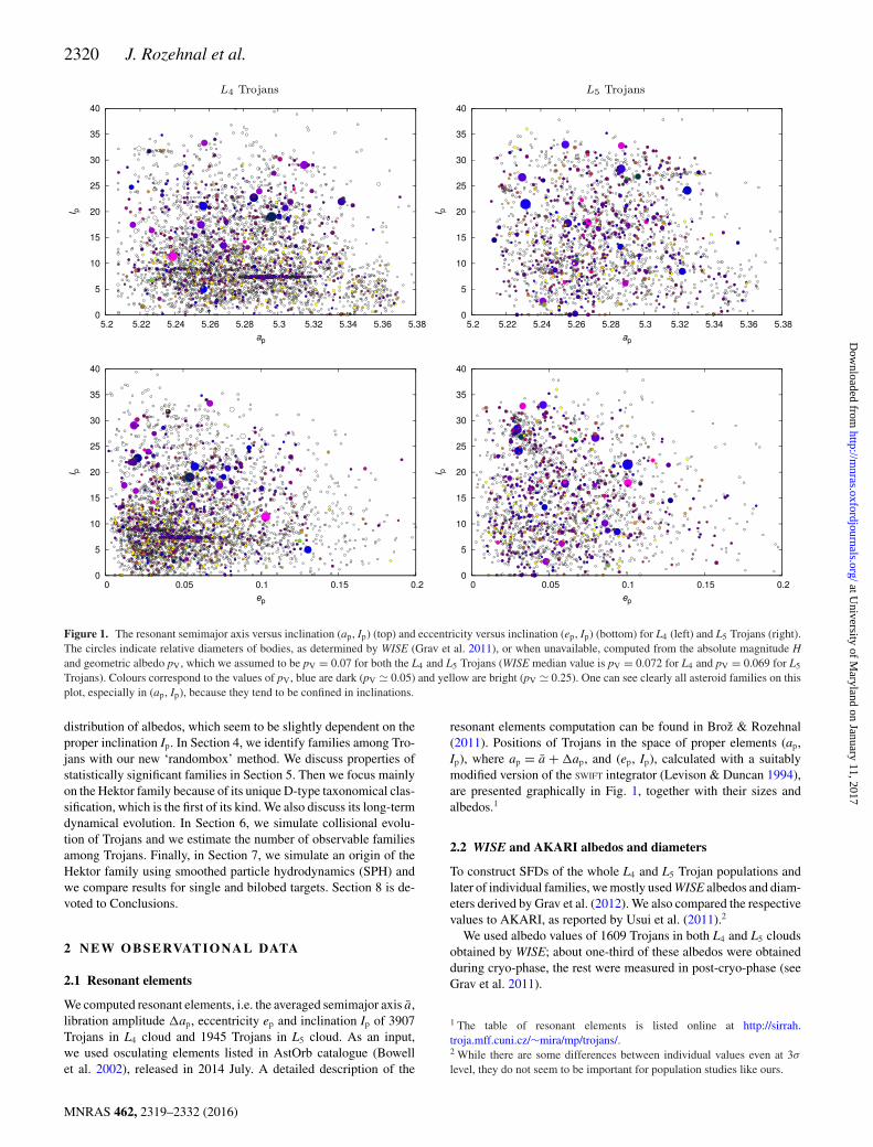
Figure 1. The resonant semimajor axis versus inclination (ap, Ip) (top) and eccentricity versus inclination (ep, Ip) (bottom) for L4 (left) and L5 Trojans (right).The circles indicate relative diameters of bodies, as determined by WISE (Grav et al. 2011), or when unavailable, computed from the absolute magnitude Hand geometric albedo pV, which we assumed to be pV = 0.07 for both the L4 and L5 Trojans (WISE median value is pV = 0.072 for L4 and pV = 0.069 for L5

Trojans). Colours correspond to the values of pV, blue are dark (pV � 0.05) and yellow are bright (pV � 0.25). One can see clearly all asteroid families on thisplot, especially in (ap, Ip), because they tend to be confined in inclinations.

distribution of albedos, which seem to be slightly dependent on theproper inclination Ip. In Section 4, we identify families among Tro-jans with our new ‘randombox’ method. We discuss properties ofstatistically significant families in Section 5. Then we focus mainlyon the Hektor family because of its unique D-type taxonomical clas-sification, which is the first of its kind. We also discuss its long-termdynamical evolution. In Section 6, we simulate collisional evolu-tion of Trojans and we estimate the number of observable familiesamong Trojans. Finally, in Section 7, we simulate an origin of theHektor family using smoothed particle hydrodynamics (SPH) andwe compare results for single and bilobed targets. Section 8 is de-voted to Conclusions.

2 N E W O B SE RVAT IO NA L DATA

2.1 Resonant elements

We computed resonant elements, i.e. the averaged semimajor axis a,libration amplitude �ap, eccentricity ep and inclination Ip of 3907Trojans in L4 cloud and 1945 Trojans in L5 cloud. As an input,we used osculating elements listed in AstOrb catalogue (Bowellet al. 2002), released in 2014 July. A detailed description of the

resonant elements computation can be found in Broz & Rozehnal(2011). Positions of Trojans in the space of proper elements (ap,Ip), where ap = a + �ap, and (ep, Ip), calculated with a suitablymodified version of the SWIFT integrator (Levison & Duncan 1994),are presented graphically in Fig. 1, together with their sizes andalbedos.1

2.2 WISE and AKARI albedos and diameters

To construct SFDs of the whole L4 and L5 Trojan populations andlater of individual families, we mostly used WISE albedos and diam-eters derived by Grav et al. (2012). We also compared the respectivevalues to AKARI, as reported by Usui et al. (2011).2

We used albedo values of 1609 Trojans in both L4 and L5 cloudsobtained by WISE; about one-third of these albedos were obtainedduring cryo-phase, the rest were measured in post-cryo-phase (seeGrav et al. 2011).

1 The table of resonant elements is listed online at http://sirrah.troja.mff.cuni.cz/∼mira/mp/trojans/.2 While there are some differences between individual values even at 3σ

level, they do not seem to be important for population studies like ours.

MNRAS 462, 2319–2332 (2016)

at University of M



ownloaded from

http://sirrah.troja.mff.cuni.cz/~mira/mp/trojans/

http://sirrah.troja.mff.cuni.cz/~mira/mp/trojans/


Hektor – an exceptional D-type family 2321

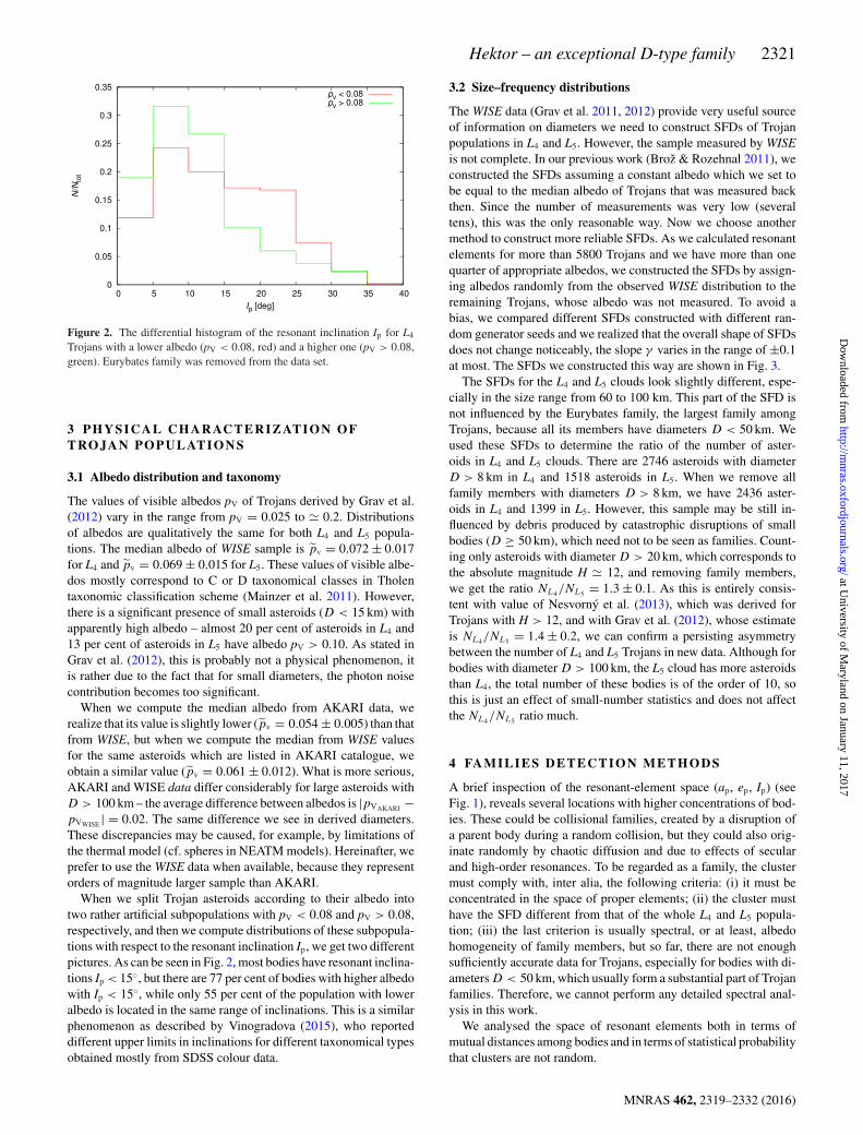
Figure 2. The differential histogram of the resonant inclination Ip for L4

Trojans with a lower albedo (pV < 0.08, red) and a higher one (pV > 0.08,green). Eurybates family was removed from the data set.

3 PH Y S I C A L C H A R AC T E R I Z AT I O N O FT RO JA N P O P U L AT I O N S

3.1 Albedo distribution and taxonomy

The values of visible albedos pV of Trojans derived by Grav et al.(2012) vary in the range from pV = 0.025 to � 0.2. Distributionsof albedos are qualitatively the same for both L4 and L5 popula-tions. The median albedo of WISE sample is pv = 0.072 ± 0.017for L4 and pv = 0.069 ± 0.015 for L5. These values of visible albe-dos mostly correspond to C or D taxonomical classes in Tholentaxonomic classification scheme (Mainzer et al. 2011). However,there is a significant presence of small asteroids (D < 15 km) withapparently high albedo – almost 20 per cent of asteroids in L4 and13 per cent of asteroids in L5 have albedo pV > 0.10. As stated inGrav et al. (2012), this is probably not a physical phenomenon, itis rather due to the fact that for small diameters, the photon noisecontribution becomes too significant.

When we compute the median albedo from AKARI data, werealize that its value is slightly lower (pv = 0.054 ± 0.005) than thatfrom WISE, but when we compute the median from WISE valuesfor the same asteroids which are listed in AKARI catalogue, weobtain a similar value (pv = 0.061 ± 0.012). What is more serious,AKARI and WISE data differ considerably for large asteroids withD > 100 km – the average difference between albedos is |pVAKARI −pVWISE | = 0.02. The same difference we see in derived diameters.These discrepancies may be caused, for example, by limitations ofthe thermal model (cf. spheres in NEATM models). Hereinafter, weprefer to use the WISE data when available, because they representorders of magnitude larger sample than AKARI.

When we split Trojan asteroids according to their albedo intotwo rather artificial subpopulations with pV < 0.08 and pV > 0.08,respectively, and then we compute distributions of these subpopula-tions with respect to the resonant inclination Ip, we get two differentpictures. As can be seen in Fig. 2, most bodies have resonant inclina-tions Ip < 15◦, but there are 77 per cent of bodies with higher albedowith Ip < 15◦, while only 55 per cent of the population with loweralbedo is located in the same range of inclinations. This is a similarphenomenon as described by Vinogradova (2015), who reporteddifferent upper limits in inclinations for different taxonomical typesobtained mostly from SDSS colour data.

3.2 Size–frequency distributions

The WISE data (Grav et al. 2011, 2012) provide very useful sourceof information on diameters we need to construct SFDs of Trojanpopulations in L4 and L5. However, the sample measured by WISEis not complete. In our previous work (Broz & Rozehnal 2011), weconstructed the SFDs assuming a constant albedo which we set tobe equal to the median albedo of Trojans that was measured backthen. Since the number of measurements was very low (severaltens), this was the only reasonable way. Now we choose anothermethod to construct more reliable SFDs. As we calculated resonantelements for more than 5800 Trojans and we have more than onequarter of appropriate albedos, we constructed the SFDs by assign-ing albedos randomly from the observed WISE distribution to theremaining Trojans, whose albedo was not measured. To avoid abias, we compared different SFDs constructed with different ran-dom generator seeds and we realized that the overall shape of SFDsdoes not change noticeably, the slope γ varies in the range of ±0.1at most. The SFDs we constructed this way are shown in Fig. 3.

The SFDs for the L4 and L5 clouds look slightly different, espe-cially in the size range from 60 to 100 km. This part of the SFD isnot influenced by the Eurybates family, the largest family amongTrojans, because all its members have diameters D < 50 km. Weused these SFDs to determine the ratio of the number of aster-oids in L4 and L5 clouds. There are 2746 asteroids with diameterD > 8 km in L4 and 1518 asteroids in L5. When we remove allfamily members with diameters D > 8 km, we have 2436 aster-oids in L4 and 1399 in L5. However, this sample may be still in-fluenced by debris produced by catastrophic disruptions of smallbodies (D ≥ 50 km), which need not to be seen as families. Count-ing only asteroids with diameter D > 20 km, which corresponds tothe absolute magnitude H � 12, and removing family members,we get the ratio NL4/NL5 = 1.3 ± 0.1. As this is entirely consis-tent with value of Nesvorny et al. (2013), which was derived forTrojans with H > 12, and with Grav et al. (2012), whose estimateis NL4/NL5 = 1.4 ± 0.2, we can confirm a persisting asymmetrybetween the number of L4 and L5 Trojans in new data. Although forbodies with diameter D > 100 km, the L5 cloud has more asteroidsthan L4, the total number of these bodies is of the order of 10, sothis is just an effect of small-number statistics and does not affectthe NL4/NL5 ratio much.

4 FA M I L I E S D E T E C T I O N M E T H O D S

A brief inspection of the resonant-element space (ap, ep, Ip) (seeFig. 1), reveals several locations with higher concentrations of bod-ies. These could be collisional families, created by a disruption ofa parent body during a random collision, but they could also orig-inate randomly by chaotic diffusion and due to effects of secularand high-order resonances. To be regarded as a family, the clustermust comply with, inter alia, the following criteria: (i) it must beconcentrated in the space of proper elements; (ii) the cluster musthave the SFD different from that of the whole L4 and L5 popula-tion; (iii) the last criterion is usually spectral, or at least, albedohomogeneity of family members, but so far, there are not enoughsufficiently accurate data for Trojans, especially for bodies with di-ameters D < 50 km, which usually form a substantial part of Trojanfamilies. Therefore, we cannot perform any detailed spectral anal-ysis in this work.

We analysed the space of resonant elements both in terms ofmutual distances among bodies and in terms of statistical probabilitythat clusters are not random.

MNRAS 462, 2319–2332 (2016)

at University of M



ownloaded from



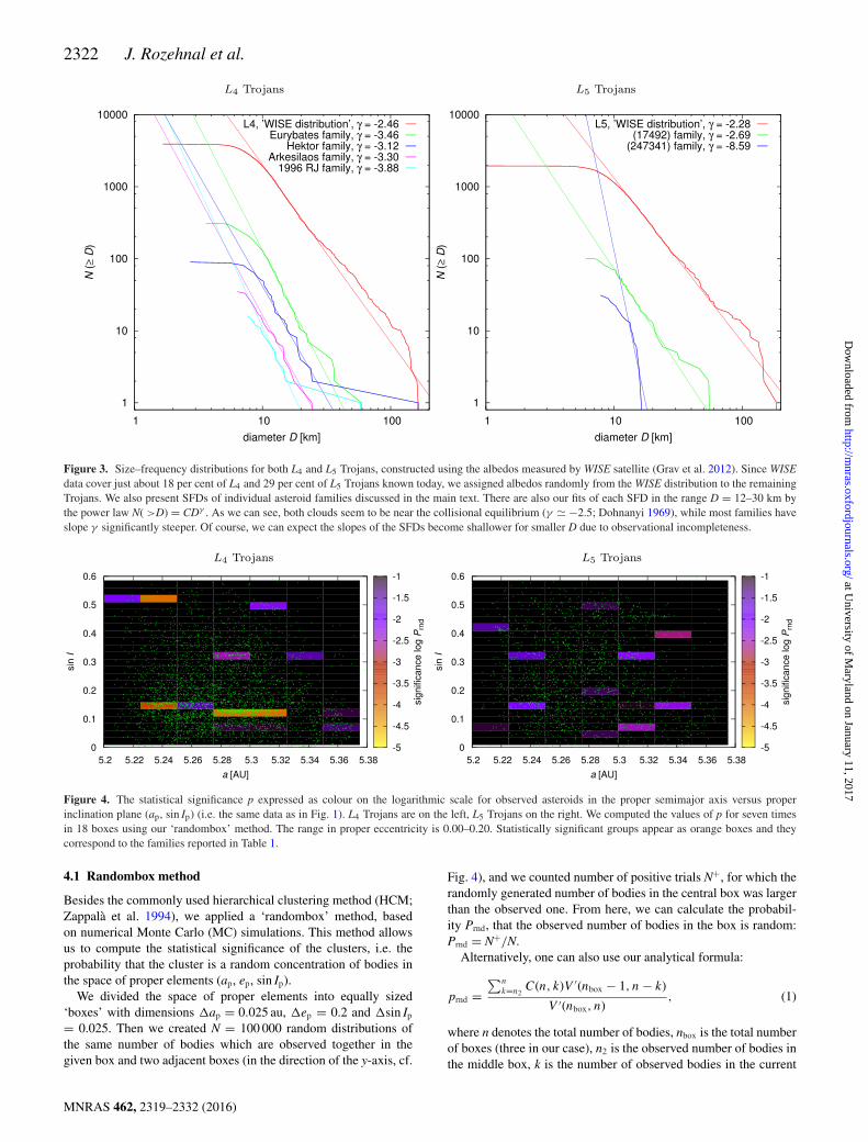
Figure 3. Size–frequency distributions for both L4 and L5 Trojans, constructed using the albedos measured by WISE satellite (Grav et al. 2012). Since WISEdata cover just about 18 per cent of L4 and 29 per cent of L5 Trojans known today, we assigned albedos randomly from the WISE distribution to the remainingTrojans. We also present SFDs of individual asteroid families discussed in the main text. There are also our fits of each SFD in the range D = 12–30 km bythe power law N( >D) = CDγ . As we can see, both clouds seem to be near the collisional equilibrium (γ � −2.5; Dohnanyi 1969), while most families haveslope γ significantly steeper. Of course, we can expect the slopes of the SFDs become shallower for smaller D due to observational incompleteness.

Figure 4. The statistical significance p expressed as colour on the logarithmic scale for observed asteroids in the proper semimajor axis versus properinclination plane (ap, sin Ip) (i.e. the same data as in Fig. 1). L4 Trojans are on the left, L5 Trojans on the right. We computed the values of p for seven timesin 18 boxes using our ‘randombox’ method. The range in proper eccentricity is 0.00–0.20. Statistically significant groups appear as orange boxes and theycorrespond to the families reported in Table 1.

4.1 Randombox method

Besides the commonly used hierarchical clustering method (HCM;Zappala et al. 1994), we applied a ‘randombox’ method, basedon numerical Monte Carlo (MC) simulations. This method allowsus to compute the statistical significance of the clusters, i.e. theprobability that the cluster is a random concentration of bodies inthe space of proper elements (ap, ep, sin Ip).

We divided the space of proper elements into equally sized‘boxes’ with dimensions �ap = 0.025 au, �ep = 0.2 and �sin Ip

= 0.025. Then we created N = 100 000 random distributions ofthe same number of bodies which are observed together in thegiven box and two adjacent boxes (in the direction of the y-axis, cf.

Fig. 4), and we counted number of positive trials N+, for which therandomly generated number of bodies in the central box was largerthan the observed one. From here, we can calculate the probabil-ity Prnd, that the observed number of bodies in the box is random:Prnd = N+/N.

Alternatively, one can also use our analytical formula:

prnd =∑n

k=n2C(n, k)V ′(nbox − 1, n − k)

V ′(nbox, n), (1)

where n denotes the total number of bodies, nbox is the total numberof boxes (three in our case), n2 is the observed number of bodies inthe middle box, k is the number of observed bodies in the current

MNRAS 462, 2319–2332 (2016)

at University of M



ownloaded from



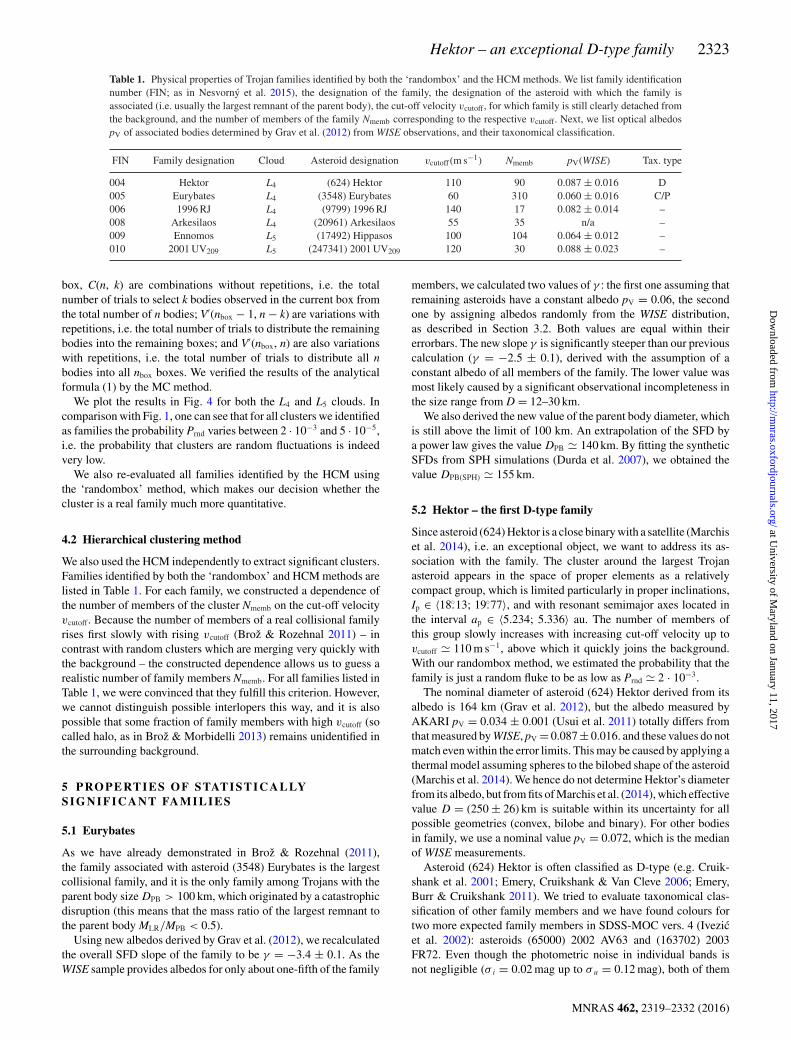
Table 1. Physical properties of Trojan families identified by both the ‘randombox’ and the HCM methods. We list family identificationnumber (FIN; as in Nesvorny et al. 2015), the designation of the family, the designation of the asteroid with which the family isassociated (i.e. usually the largest remnant of the parent body), the cut-off velocity vcutoff, for which family is still clearly detached fromthe background, and the number of members of the family Nmemb corresponding to the respective vcutoff. Next, we list optical albedospV of associated bodies determined by Grav et al. (2012) from WISE observations, and their taxonomical classification.

FIN Family designation Cloud Asteroid designation vcutoff (m s−1) Nmemb pV(WISE) Tax. type

004 Hektor L4 (624) Hektor 110 90 0.087 ± 0.016 D005 Eurybates L4 (3548) Eurybates 60 310 0.060 ± 0.016 C/P006 1996 RJ L4 (9799) 1996 RJ 140 17 0.082 ± 0.014 –008 Arkesilaos L4 (20961) Arkesilaos 55 35 n/a –009 Ennomos L5 (17492) Hippasos 100 104 0.064 ± 0.012 –010 2001 UV209 L5 (247341) 2001 UV209 120 30 0.088 ± 0.023 –

box, C(n, k) are combinations without repetitions, i.e. the totalnumber of trials to select k bodies observed in the current box fromthe total number of n bodies; V′(nbox − 1, n − k) are variations withrepetitions, i.e. the total number of trials to distribute the remainingbodies into the remaining boxes; and V′(nbox, n) are also variationswith repetitions, i.e. the total number of trials to distribute all nbodies into all nbox boxes. We verified the results of the analyticalformula (1) by the MC method.

We plot the results in Fig. 4 for both the L4 and L5 clouds. Incomparison with Fig. 1, one can see that for all clusters we identifiedas families the probability Prnd varies between 2 · 10−3 and 5 · 10−5,i.e. the probability that clusters are random fluctuations is indeedvery low.

We also re-evaluated all families identified by the HCM usingthe ‘randombox’ method, which makes our decision whether thecluster is a real family much more quantitative.

4.2 Hierarchical clustering method

We also used the HCM independently to extract significant clusters.Families identified by both the ‘randombox’ and HCM methods arelisted in Table 1. For each family, we constructed a dependence ofthe number of members of the cluster Nmemb on the cut-off velocityvcutoff. Because the number of members of a real collisional familyrises first slowly with rising vcutoff (Broz & Rozehnal 2011) – incontrast with random clusters which are merging very quickly withthe background – the constructed dependence allows us to guess arealistic number of family members Nmemb. For all families listed inTable 1, we were convinced that they fulfill this criterion. However,we cannot distinguish possible interlopers this way, and it is alsopossible that some fraction of family members with high vcutoff (socalled halo, as in Broz & Morbidelli 2013) remains unidentified inthe surrounding background.

5 PRO PERTIES O F STATISTICALLYSIGNIFICANT FA MILIES

5.1 Eurybates

As we have already demonstrated in Broz & Rozehnal (2011),the family associated with asteroid (3548) Eurybates is the largestcollisional family, and it is the only family among Trojans with theparent body size DPB > 100 km, which originated by a catastrophicdisruption (this means that the mass ratio of the largest remnant tothe parent body MLR/MPB < 0.5).

Using new albedos derived by Grav et al. (2012), we recalculatedthe overall SFD slope of the family to be γ = −3.4 ± 0.1. As theWISE sample provides albedos for only about one-fifth of the family

members, we calculated two values of γ : the first one assuming thatremaining asteroids have a constant albedo pV = 0.06, the secondone by assigning albedos randomly from the WISE distribution,as described in Section 3.2. Both values are equal within theirerrorbars. The new slope γ is significantly steeper than our previouscalculation (γ = −2.5 ± 0.1), derived with the assumption of aconstant albedo of all members of the family. The lower value wasmost likely caused by a significant observational incompleteness inthe size range from D = 12–30 km.

We also derived the new value of the parent body diameter, whichis still above the limit of 100 km. An extrapolation of the SFD bya power law gives the value DPB � 140 km. By fitting the syntheticSFDs from SPH simulations (Durda et al. 2007), we obtained thevalue DPB(SPH) � 155 km.

5.2 Hektor – the first D-type family

Since asteroid (624) Hektor is a close binary with a satellite (Marchiset al. 2014), i.e. an exceptional object, we want to address its as-sociation with the family. The cluster around the largest Trojanasteroid appears in the space of proper elements as a relativelycompact group, which is limited particularly in proper inclinations,Ip ∈ 〈18.◦13; 19.◦77〉, and with resonant semimajor axes located inthe interval ap ∈ 〈5.234; 5.336〉 au. The number of members ofthis group slowly increases with increasing cut-off velocity up tovcutoff � 110 m s−1, above which it quickly joins the background.With our randombox method, we estimated the probability that thefamily is just a random fluke to be as low as Prnd � 2 · 10−3.

The nominal diameter of asteroid (624) Hektor derived from itsalbedo is 164 km (Grav et al. 2012), but the albedo measured byAKARI pV = 0.034 ± 0.001 (Usui et al. 2011) totally differs fromthat measured by WISE, pV = 0.087 ± 0.016. and these values do notmatch even within the error limits. This may be caused by applying athermal model assuming spheres to the bilobed shape of the asteroid(Marchis et al. 2014). We hence do not determine Hektor’s diameterfrom its albedo, but from fits of Marchis et al. (2014), which effectivevalue D = (250 ± 26) km is suitable within its uncertainty for allpossible geometries (convex, bilobe and binary). For other bodiesin family, we use a nominal value pV = 0.072, which is the medianof WISE measurements.

Asteroid (624) Hektor is often classified as D-type (e.g. Cruik-shank et al. 2001; Emery, Cruikshank & Van Cleve 2006; Emery,Burr & Cruikshank 2011). We tried to evaluate taxonomical clas-sification of other family members and we have found colours fortwo more expected family members in SDSS-MOC vers. 4 (Ivezicet al. 2002): asteroids (65000) 2002 AV63 and (163702) 2003FR72. Even though the photometric noise in individual bands isnot negligible (σ i = 0.02 mag up to σ u = 0.12 mag), both of them

MNRAS 462, 2319–2332 (2016)

at University of M



ownloaded from



are D-types, with principal components (also known as slopes)PC1 >0.3. This seems to support the D-type classification of thewhole family.

We also tried to constrain the taxonomic classification of thefamily members by comparing their infrared (IR) albedos pIR andvisual albedos pV as described in Mainzer et al. (2011), but thereare no data for family members in the W1 or W2 band of the WISEsample, which are dominated by reflected radiation.

The fact that we observe a collisional family associated witha D-type asteroid is the main reason we use word ‘exceptional’in connection with the Hektor family. As we claimed in Brozet al. (2013), in all regions containing a mixture of C-type and D-type asteroids (e.g. Trojans, Hildas, Cybeles), there have been onlyC-type families observed so far, which could indicate that disrup-tions of D-type asteroids leave no family behind, as suggested byLevison et al. (2009). Nevertheless, our classification of the Hektorfamily as D-type is not in direct contradiction with this conclusion,because Levison et al. (2009) were concerned with catastrophic dis-ruptions, while we conclude below that the Hektor family originatedfrom a cratering event, i.e. by an impactor with kinetic energy toosmall to disrupt the parent body.

5.2.1 Simulations of long-term dynamical evolution

To get an upper limit of the age of the Hektor family, we simulated along-term evolution of seven synthetic families created for differentbreakup geometries. Our model included four giant planets on cur-rent orbits, integrated by the symplectic integrator SWIFT (Levison& Duncan 1994), modified according to Laskar & Robutel (2001),with the timestep of �t = 91 d and timespan 4 Gyr.

We also accounted for the Yarkovsky effect in our simulations.Although in a first-order theory, it is not effective in zero-order reso-nances (it could just shift libration centre, but there is no systematicdrift in semimajor axis) and the observed evolution of proper ele-ments is mainly due to chaotic diffusion, in higher order theories,the Yarkovsky effect can play some role. In our model, we assumeda random distribution of spins and rotation periods (typically severalhours), the bulk and surface density ρbulk = ρsurf = 1.3 g cm−3, thethermal conductivity K = 0.01 W m−1 K−1, the specific heat ca-pacity C = 680 J kg−1 K−1, the Bond albedo AB = 0.02 and the IRemissivity ε = 0.95.

We created each synthetic family by assigning random velocitiesto 234 bodies (i.e. three times more than the number of the observedfamily members), assuming an isotropic velocity field with a typicalvelocity of 70 m s−1, corresponding to the escape velocity fromparent body (Farinella, Froeschle & Gonczi 1994). Here we assumedthe velocity of fragments to be size independent. Possible trends inthe ejection velocity field cannot be easily revealed in the (a, H)space in the case of the Hektor family, because of its origin by acratering event – there is a large gap in the range between absolutemagnitude of (624) Hektor (H = 7.20) and other bodies (H > 11.9),so we are not able to distinguish a simple Gaussian dispersion fromthe physical dependence (cf. Carruba & Nesvorny 2016). Eitherway, we are interested in the orbital distribution of mostly smallbodies. Our assumption of size-independent ejection velocity isalso in good agreement with results of SPH models (see subsection7.3 and Fig. 13).

To create a synthetic family in the same position as occupiedby the observed Hektor family, we integrated the orbit of asteroid(624) Hektor with osculating elements taken from AstOrb cata-logue (Bowell et al. 2002), until we got appropriate values of the

true anomaly f and the argument of pericentre ω. We tried valuesof f ranging from 0◦ to 180◦ with the step of 30◦ and ω alwayssatisfying the condition f + ω = 60◦, i.e. we fixed the angular dis-tance from the node to ensure a comparably large perturbations ininclinations.

Initial positions of synthetic families members just after the dis-ruption, compared to the observed Hektor family, are shown inFig. 5. To make a quantitative comparison of the distribution in thespace of proper elements, we used a two-dimensional Kolmogorov–Smirnov (KS) test to compute KS distance of the synthetic familyto the observed one with the output timestep of 1 Myr. The resultsfor different initial geometries are shown in Fig. 6.

Our two best fits corresponding to the lowest KS distanceare displayed in Fig. 7. As we can see from the image of thewhole Trojan L4 population, Hektor seems to be near the out-skirts of the librating region (cf. Fig. 1). In Fig. 5, we can notethat there are almost no observed asteroids in the shaded area withap > 5.32 au, but we can see some synthetic family members in theleft-hand panel of Fig. 7 (initial geometry f = 0◦, ω = 60◦).

On the other hand, when we look at right-hand panel of Fig. 7(initial geometry f = 150◦, ω = 270◦), we can see that there aremany fewer bodies in the proximity of the border of the stablelibrating region. One can also see the initial ‘fibre-like’ structure isstill visible on the left, but is almost dispersed on the right.

Hence, we conclude that the geometry at which the disruptionoccurred is rather f = 150◦, ω = 270◦ and the corresponding age isbetween 1 and 4 Gyr. The second but less likely possibility is thatthe disruption could have occurred more recently (0.1–2.5 Gyr) atf = 0◦, ω = 60◦.

5.2.2 Parent body size from SPH simulations

We tried to estimate the parent body size of Hektor family and otherfamilies by the method described in Durda et al. (2007). To thispoint, we calculated a pseudo−χ2 for the whole set of syntheticSFDs as given by the SPH simulations results (see Fig. 8).

Parent body sizes DPB(SPH) and mass ratios of the largest fragmentand parent body MLF/MPB estimated by this method are listed inTable 2. The parent body size for Hektor family we derivedfrom SPH simulations is DPB(SPH) = (260 ± 10) km, the impactordiameter Dimp = (24 ± 2) km, the impactor velocity vimp = (4 ±1) km s−1 and the impact angle ϕimp = (60◦ ± 15◦). We will use thesevalues as initial conditions for simulations of collisional evolutionbelow.

5.3 1996 RJ – extremely compact family

In our previous work, we mentioned a small cluster associated withasteroid (9799) 1996 RJ, which consisted of just nine bodies. Withthe contemporary sample of resonant elements, we can confirm thatthis cluster is indeed visible. It is composed of 18 bodies situatednear the edge of the librating zone on high inclinations, within theranges Ip ∈ 〈31.◦38; 32.◦27〉 and ap ∈ 〈5.225 ; 5.238〉 au. As it isdetached from the background in the space of proper elements, itremains isolated even at high cut-off velocity vcutoff = 160 m s−1.

Unfortunately, we have albedos measured by WISE for just fourmembers of this family. These albedos are not much dispersed. Theyrange from pV = 0.079 ± 0.019 to 0.109 ± 0.029 and, compared tothe median albedo of the whole L4 population pV = 0.072 ± 0.017,they seem to be a bit brighter, but this statement is a bit inconclusive.

MNRAS 462, 2319–2332 (2016)

at University of M



ownloaded from



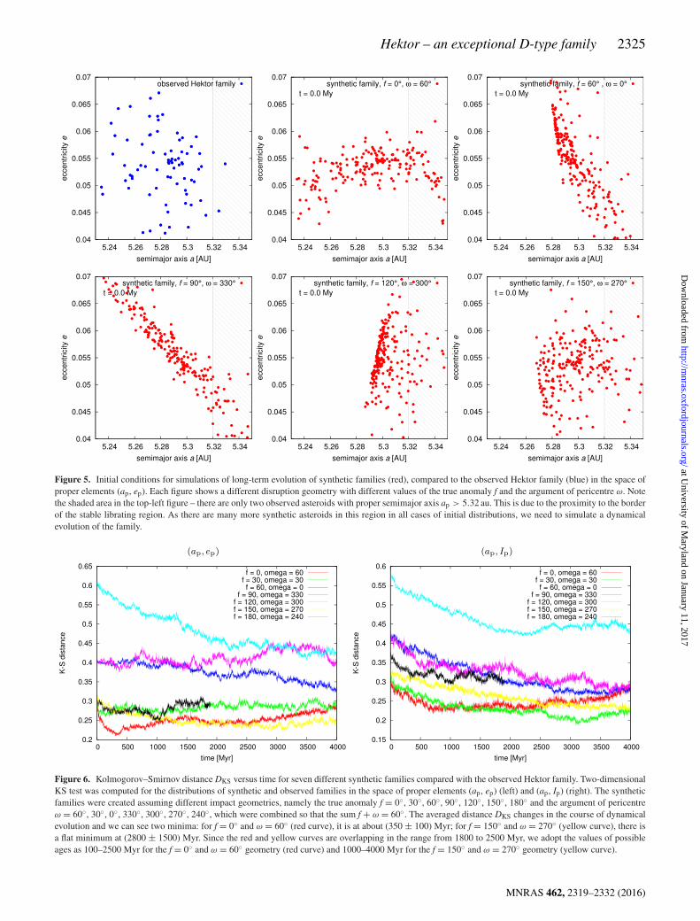
Figure 5. Initial conditions for simulations of long-term evolution of synthetic families (red), compared to the observed Hektor family (blue) in the space ofproper elements (ap, ep). Each figure shows a different disruption geometry with different values of the true anomaly f and the argument of pericentre ω. Notethe shaded area in the top-left figure – there are only two observed asteroids with proper semimajor axis ap > 5.32 au. This is due to the proximity to the borderof the stable librating region. As there are many more synthetic asteroids in this region in all cases of initial distributions, we need to simulate a dynamicalevolution of the family.

Figure 6. Kolmogorov–Smirnov distance DKS versus time for seven different synthetic families compared with the observed Hektor family. Two-dimensionalKS test was computed for the distributions of synthetic and observed families in the space of proper elements (ap, ep) (left) and (ap, Ip) (right). The syntheticfamilies were created assuming different impact geometries, namely the true anomaly f = 0◦, 30◦, 60◦, 90◦, 120◦, 150◦, 180◦ and the argument of pericentreω = 60◦, 30◦, 0◦, 330◦, 300◦, 270◦, 240◦, which were combined so that the sum f + ω = 60◦. The averaged distance DKS changes in the course of dynamicalevolution and we can see two minima: for f = 0◦ and ω = 60◦ (red curve), it is at about (350 ± 100) Myr; for f = 150◦ and ω = 270◦ (yellow curve), there isa flat minimum at (2800 ± 1500) Myr. Since the red and yellow curves are overlapping in the range from 1800 to 2500 Myr, we adopt the values of possibleages as 100–2500 Myr for the f = 0◦ and ω = 60◦ geometry (red curve) and 1000–4000 Myr for the f = 150◦ and ω = 270◦ geometry (yellow curve).

MNRAS 462, 2319–2332 (2016)

at University of M



ownloaded from



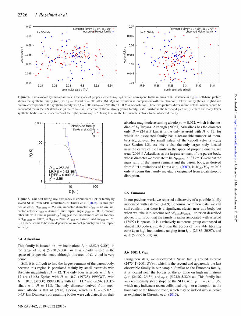
Figure 7. Two evolved synthetic families in the space of proper elements (ap, ep), which correspond to the minima of KS distance in Fig. 6. Left-hand pictureshows the synthetic family (red) with f = 0◦ and ω = 60◦ after 364 Myr of evolution in comparison with the observed Hektor family (blue). Right-handpicture corresponds to the synthetic family with f = 150◦ and ω = 270◦ after 3100 Myr of evolution. These two pictures differ in fine details, which cannot beaccounted for in the KS statistics: (i) the ‘fibre-like’ structure of the relatively young family is still visible in the left-hand picture; (ii) there are many fewersynthetic bodies in the shaded area of the right picture (ap > 5.32 au) than on the left, which is closer to the observed reality.

Figure 8. Our best-fitting size–frequency distribution of Hektor family byscaled SFDs from SPH simulations of Durda et al. (2007). In this par-ticular case, DPB(SPH) = 257 km, impactor diameter Dimp = 48 km, im-pactor velocity vimp = 4 km s−1 and impact angle ϕimp = 60◦. However,other fits with similar pseudo-χ2 suggest the uncertainties are as follows:�DPB(SPH) = 10 km, �Dimp = 2 km, �vimp = 1 km s−1 and �ϕimp = 15◦.SFD shape seems to be more dependent on impact geometry than on impactvelocity.

5.4 Arkesilaos

This family is located on low inclinations Ip ∈ 〈8.52◦; 9.20◦〉, inthe range of ap ∈ 〈5.230 ; 5.304〉 au. It is clearly visible in thespace of proper elements, although this area of L4 cloud is verydense.

Still, it is difficult to find the largest remnant of the parent body,because this region is populated mainly by small asteroids withabsolute magnitudes H > 12. The only four asteroids with H <

12 are (2148) Epeios with H = 10.7, (19725) 1999 WT4 withH = 10.7, (38600) 1999 XR213 with H = 11.7 and (20961) Arke-silaos with H = 11.8. The only diameter derived from mea-sured albedo is that of (2148) Epeios, which is D = (39.02 ±0.65) km. Diameters of remaining bodies were calculated from their

absolute magnitude assuming albedo pV = 0.072, which is the me-dian of L4 Trojans. Although (20961) Arkesilaos has the diameteronly D = (24 ± 5) km, it is the only asteroid with H < 12, forwhich the associated family has a reasonable number of mem-bers Nmemb even for small values of the cut-off velocity vcutoff

(see Section 4.2). As this is also the only larger body locatednear the centre of the family in the space of proper elements, wetreat (20961) Arkesilaos as the largest remnant of the parent body,whose diameter we estimate to be DPB(SPH) � 87 km. Given that themass ratio of the largest remnant and the parent body, as derivedfrom SPH simulations of Durda et al. (2007), is MLR/MPB � 0.02only, it seems this family inevitably originated from a catastrophicdisruption.

5.5 Ennomos

In our previous work, we reported a discovery of a possible familyassociated with asteroid (4709) Ennomos. With new data, we canstill confirm that there is a significant cluster near this body, butwhen we take into account our ‘Nmemb(vcutoff)’ criterion describedabove, it turns out that the family is rather associated with asteroid(17492) Hippasos. It is a relatively numerous group composed ofalmost 100 bodies, situated near the border of the stable libratingzone L5 at high inclinations, ranging from Ip ∈ 〈26.◦86; 30.◦97〉, andap ∈ 〈5.225; 5.338〉 au.

5.6 2001 UV209

Using new data, we discovered a ‘new’ family around asteroid(247341) 2001 UV209, which is the second and apparently the lastobservable family in our sample. Similar to the Ennomos family,it is located near the border of the L5 zone on high inclinationsIp ∈ 〈24.◦02; 26.◦56〉 and ap ∈ 〈5.218; 5.320〉 au. This family hasan exceptionally steep slope of the SFD, with γ = −8.6 ± 0.9,which may indicate a recent collisional origin or a disruption at theboundary of the libration zone, which may be indeed size-selectiveas explained in Chrenko et al. (2015).

MNRAS 462, 2319–2332 (2016)

at University of M



ownloaded from



Table 2. Derived properties of Trojan families. We list here the family designation, the diameter of the largest remnant DLR, the minimaldiameter of the parent body min DPB, obtained as the sum of all observed family members, the diameter of the parent body DPB(SPH) and themass ratio MLR/MPB of the largest fragment and the parent body, both derived from our fits by scaled SPH simulations performed by Durdaet al. (2007). We use this ratio to distinguish between the catastrophic disruption (MLR/MPB < 0.5) and the cratering (MLR/MPB > 0.5). Finally,there is the escape velocity vesc from the parent body and estimated age of the family derived in this and our previous work (Broz & Rozehnal2011).

Family designation DLR (km) min DPB DPB(SPH) MLR/MPB vesc(m s−1) Age (Gyr) Notes, references

Hektor 250 ± 26 250 257 0.92 73 0.3–3 1, 3Eurybates 59.4 ± 1.5 100 155 0.06 46 1.0–3.8 21996 RJ 58.3 ± 0.9 61 88 0.29 26 – 2, 4Arkesilaos 24 ± 5 37 87 0.02 16 – 2Ennomos 55.2 ± 0.9 67–154 95–168 0.04–0.19 29–66 1–2 2, 52001 UV209 16.3 ± 1.1 32 80 0.01 14 – 2

Notes. 1DLR derived by Marchis et al. (2014),2DLR derived by Grav et al. (2012),3bilobe, satellite (Marchis et al. 2014),4very compact, Broz & Rozehnal (2011),5DPB strongly influenced by interlopers,6The largest fragment of Ennomos family is (17492) Hippasos.

Figure 9. Simulations of the collisional evolution of L4 Trojans with theBoulder code (Morbidelli et al. 2009). Shown here is the initial cumulativeSFD of a synthetic population (black) and the SFD of the observed one (red).Green are the final SFDs of 100 synthetic populations with the same initialSFD but with different random seeds, after 4 Gyr of a collisional evolution.The evolution of bodies larger than D > 50 km is very slow, hence we canconsider this part of the SFD as captured population.

6 C O L L I S I O NA L M O D E L S O F T H E T RO JA NP O P U L AT I O N

In order to estimate the number of collisional families among L4

Trojans, we performed a set of 100 simulations of the collisionalevolution of Trojans with the Boulder code (Morbidelli et al. 2009)with the same initial conditions, but with different values of therandom seed.

6.1 Initial conditions

We set our initial conditions of the simulations such that 4 Gyr ofcollisional evolution leads to the observed cumulative SFD of L4

Trojans (red curve in Fig. 9). We constructed the initial syntheticSFD as three power laws with the slopes γ a = −6.60 in the sizerange from D1 = 117 km to Dmax = 250 km, γ b = −3.05 fromD2 = 25 km to D1 and γ c = −3.70 from Dmin = 0.05 km to D2.

The synthetic initial population was normalized to contain Nnorm =11 asteroids with diameters D ≥ D1.

To calculate the target strength Q∗D , we used a parametric formula

of Benz & Asphaug (1999):

Q∗D = Q0R

aPB + BρbulkR

bPB, (2)

where RPB is the parent body radius in centimetres, ρbulk its bulkdensity, which we set to be ρbulk = 1.3 g cm−3 for synthetic Trojans(cf. Marchis et al. 2014). As of constants a, b, B and Q0, we usedthe values determined by Benz & Asphaug (1999) for ice at theimpact velocity vimp = 3 km s−1, which are a = −0.39, b = 1.26,B = 1.2 erg cm3 g−2 and Q0 = 1.6 · 107 erg g−1.

In our model, we take into account only Trojan versus Trojancollisions, as the Trojan region is practically detached from themain belt. Anyway, main-belt asteroids with eccentricities largeenough to reach the Trojan region are usually scattered by Jupiteron a time-scale significantly shorter than the average time neededto collide with a relatively large Trojan asteroid. We thus assumedthe values of collisional probability Pi = 7.80 · 10−18 km−2 yr−1

and the impact velocity vimp = 4.66 km s−1 (Dell’Oro et al. 1998).Unfortunately, Benz & Asphaug (1999) do not provide parametersfor ice at the impact velocities vimp > 3 km s−1.

We also ran several simulations with appropriate values for basaltat impact velocity vimp = 5 km s−1 (a = −0.36, b = 1.36, B =0.5 erg cm3 g−2 and Q0 = 9 · 107 erg g−1).

Both models qualitatively exhibit the same evolution of SFD andthey give approximately the same total numbers of disruptions andcraterings occurred, but for basalt, the model gives three times fewerobservable families originated by cratering than for ice. The resultsfor the ice match the observation better, so we will further discussthe results for ice only.

6.2 Long-term collisional evolution

The results of our simulations of the collisional evolution are shownin Fig. 9. Our collisional model shows only little changes aboveD > 50 km over the last 3.85 Gyr (i.e. post-LHB phase only). Slopesof the initial synthetic population and the observed L4 populationdiffer by �γ < 0.1 in the size range from 50 to 100 km, whilea relative decrease of the number of asteroids after 3.85 Gyr ofcollisional evolution is only about 12 per cent in the same size

MNRAS 462, 2319–2332 (2016)

at University of M



ownloaded from



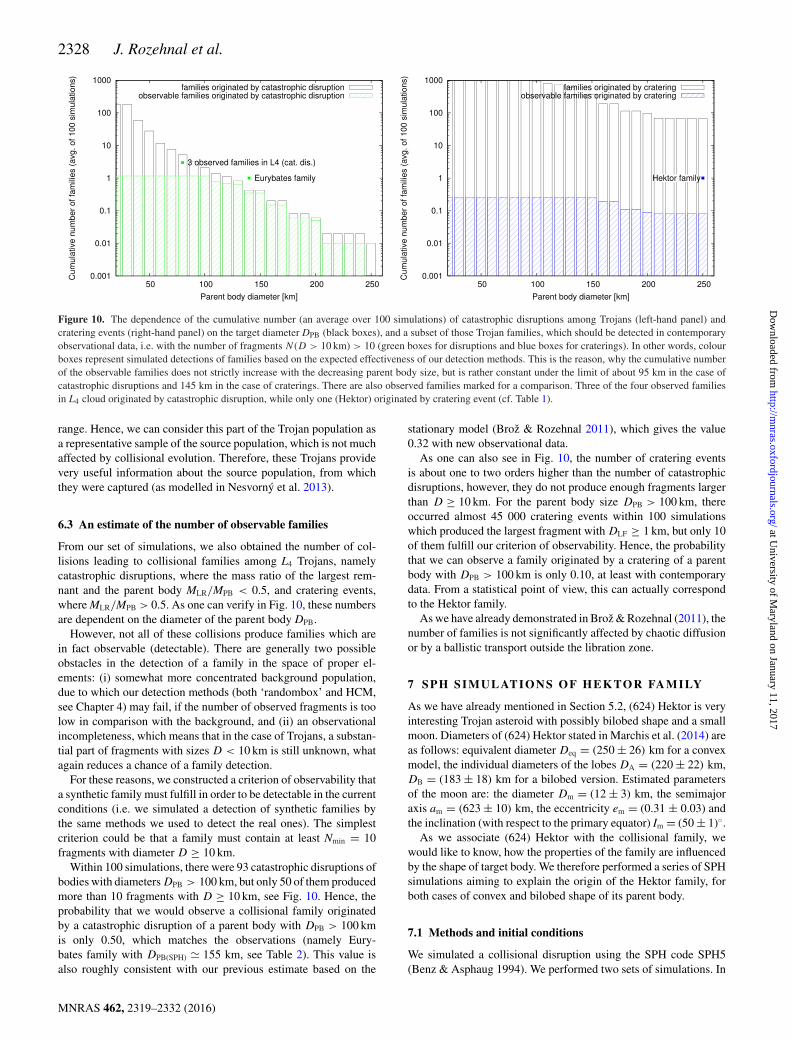
Figure 10. The dependence of the cumulative number (an average over 100 simulations) of catastrophic disruptions among Trojans (left-hand panel) andcratering events (right-hand panel) on the target diameter DPB (black boxes), and a subset of those Trojan families, which should be detected in contemporaryobservational data, i.e. with the number of fragments N (D > 10 km) > 10 (green boxes for disruptions and blue boxes for craterings). In other words, colourboxes represent simulated detections of families based on the expected effectiveness of our detection methods. This is the reason, why the cumulative numberof the observable families does not strictly increase with the decreasing parent body size, but is rather constant under the limit of about 95 km in the case ofcatastrophic disruptions and 145 km in the case of craterings. There are also observed families marked for a comparison. Three of the four observed familiesin L4 cloud originated by catastrophic disruption, while only one (Hektor) originated by cratering event (cf. Table 1).

range. Hence, we can consider this part of the Trojan population asa representative sample of the source population, which is not muchaffected by collisional evolution. Therefore, these Trojans providevery useful information about the source population, from whichthey were captured (as modelled in Nesvorny et al. 2013).

6.3 An estimate of the number of observable families

From our set of simulations, we also obtained the number of col-lisions leading to collisional families among L4 Trojans, namelycatastrophic disruptions, where the mass ratio of the largest rem-nant and the parent body MLR/MPB < 0.5, and cratering events,where MLR/MPB > 0.5. As one can verify in Fig. 10, these numbersare dependent on the diameter of the parent body DPB.

However, not all of these collisions produce families which arein fact observable (detectable). There are generally two possibleobstacles in the detection of a family in the space of proper el-ements: (i) somewhat more concentrated background population,due to which our detection methods (both ‘randombox’ and HCM,see Chapter 4) may fail, if the number of observed fragments is toolow in comparison with the background, and (ii) an observationalincompleteness, which means that in the case of Trojans, a substan-tial part of fragments with sizes D < 10 km is still unknown, whatagain reduces a chance of a family detection.

For these reasons, we constructed a criterion of observability thata synthetic family must fulfill in order to be detectable in the currentconditions (i.e. we simulated a detection of synthetic families bythe same methods we used to detect the real ones). The simplestcriterion could be that a family must contain at least Nmin = 10fragments with diameter D ≥ 10 km.

Within 100 simulations, there were 93 catastrophic disruptions ofbodies with diameters DPB > 100 km, but only 50 of them producedmore than 10 fragments with D ≥ 10 km, see Fig. 10. Hence, theprobability that we would observe a collisional family originatedby a catastrophic disruption of a parent body with DPB > 100 kmis only 0.50, which matches the observations (namely Eury-bates family with DPB(SPH) � 155 km, see Table 2). This value isalso roughly consistent with our previous estimate based on the

stationary model (Broz & Rozehnal 2011), which gives the value0.32 with new observational data.

As one can also see in Fig. 10, the number of cratering eventsis about one to two orders higher than the number of catastrophicdisruptions, however, they do not produce enough fragments largerthan D ≥ 10 km. For the parent body size DPB > 100 km, thereoccurred almost 45 000 cratering events within 100 simulationswhich produced the largest fragment with DLF ≥ 1 km, but only 10of them fulfill our criterion of observability. Hence, the probabilitythat we can observe a family originated by a cratering of a parentbody with DPB > 100 km is only 0.10, at least with contemporarydata. From a statistical point of view, this can actually correspondto the Hektor family.

As we have already demonstrated in Broz & Rozehnal (2011), thenumber of families is not significantly affected by chaotic diffusionor by a ballistic transport outside the libration zone.

7 SPH SI MULATI ONS O F H EKTO R FAMI LY

As we have already mentioned in Section 5.2, (624) Hektor is veryinteresting Trojan asteroid with possibly bilobed shape and a smallmoon. Diameters of (624) Hektor stated in Marchis et al. (2014) areas follows: equivalent diameter Deq = (250 ± 26) km for a convexmodel, the individual diameters of the lobes DA = (220 ± 22) km,DB = (183 ± 18) km for a bilobed version. Estimated parametersof the moon are: the diameter Dm = (12 ± 3) km, the semimajoraxis am = (623 ± 10) km, the eccentricity em = (0.31 ± 0.03) andthe inclination (with respect to the primary equator) Im = (50 ± 1)◦.

As we associate (624) Hektor with the collisional family, wewould like to know, how the properties of the family are influencedby the shape of target body. We therefore performed a series of SPHsimulations aiming to explain the origin of the Hektor family, forboth cases of convex and bilobed shape of its parent body.

7.1 Methods and initial conditions

We simulated a collisional disruption using the SPH code SPH5(Benz & Asphaug 1994). We performed two sets of simulations. In

MNRAS 462, 2319–2332 (2016)

at University of M



ownloaded from



Table 3. Material constants used in our SPH simulations for basalt and sili-cated ice (30 per cent of silicates). Listed here are: the zero-pressure densityρ0, bulk modulus A, non-linear compressive term B, sublimation energy E0,Tillotson parameters a, b, α and β, specific energy of incipient vaporizationEiv, complete vaporization Ecv, shear modulus μ, plastic yielding Y, meltenergy Emelt and Weibull fracture parameters k and m. Values we used forsilicated ice are identical to those of pure ice, except density ρ0, bulk mod-ulus A and Weibull parameters k and m. All values were adopted from Benz& Asphaug (1999).

Quantity Basalt Silicated ice Unit

ρ0 2.7 1.1 g cm−3

A 2.67 · 1011 8.44 · 1010 erg cm−3

B 2.67 · 1011 1.33 · 1011 erg cm−3

E0 4.87 · 1012 1.00 · 1011 erg g−1

a 0.5 0.3 –b 1.5 0.1 –α 5.0 10.0 –β 5.0 5.0 –Eiv 4.72 · 1010 7.73 · 109 erg g−1

Ecv 1.82 · 1011 3.04 · 1010 erg g−1

μ 2.27 · 1011 2.80 · 1010 erg cm−3

Y 3.5 · 1010 1.0 · 1010 erg g−1

Emelt 3.4 · 1010 7.0 · 109 erg g−1

k 4.0 · 1029 5.6 · 1038 cm−3

m 9.0 9.4 –

the first one, we simulated an impact on a single spherical asteroid.In the second, on a bilobed asteroid represented by two spherespositioned next to each other. The two touching spheres have anarrow interface, so that the SPH quantities do not easily propagatebetween them. In this setup, we are likely to see differences betweensinlge/bilobed cases as clearly as possible.

As for the main input parameters (target/impactor sizes, the im-pact velocity and the impact angle), we took the parameters of ourbest-fitting SFDs, obtained by Durda et al. (2007) scaling method,see Section 5.2.2 and Fig. 8.

To simulate a collision between the parent body and the impactor,we performed a limited set of simulations: (i) a single sphericalbasalt target with diameter DPB = 260 km versus a basalt impactorwith diameter Dimp = 48 km; (ii) the single basalt target DPB =260 km versus an ice impactor (a mixture of ice and 30 per cent ofsilicates) with Dimp = 64 km (impactor diameter was scaled to getthe same kinetic energy); (iii) a bilobed basalt target approximatedby two spheres with diameters DPB = 200 km each (the total massis approximately the same) versus a basalt impactor with Dimp =48 km; (iv) a single spherical ice target DPB = 260 km versus anice impactor Dimp = 38 km (impactor diameter was scaled to getthe same ratio of the specific kinetic energy Q to the target strengthQ∗

D).The integration was controlled by the Courant number C = 1.0,

a typical timestep thus was �t � 10−5 s, and the timespan waststop = 100 s. The Courant condition was the same in different ma-terials, using always the maximum sound speed cs among all SPHparticles, as usually.

We used NSPH,st = 105 SPH particles for the single sphericaltarget and NSPH, bt = 2 · 105 for the bilobed one. For impactorNSPH, i = 103 SPH particles. We assumed the Tillotson equation ofstate (Tillotson 1962) and material properties, which are listed inTable 3.

We terminated SPH simulations after 100 s from the impact. Thistime interval is needed to establish a velocity field of fragmentsand to complete the fragmentation. Then we handed the output of

Figure 11. A comparison of size–frequency distributions of the ob-served Hektor family (red dotted) and SFDs of synthetic families cre-ated by different SPH simulations, always assuming the impactor velocityvimp = 4 km s−1 and the impact angle ϕimp = 60◦. For a single sphericaltarget (green lines), we assumed the diameter DPB = 260 km; for a bilobetarget (blue line), we approximated the lobes as spheres with diametersDPB = 200 km each. The impactor size was assumed to be Dimp = 48 kmin the case of basalt, Dimp = 64 km in the case of silicate ice impactingon basalt target (scaled to the same Eimp) and Dimp = 38 km in the case ofsilicate ice impacting on ice target (scaled to the same Q/Q∗

D). Fragments ofthe impactor were purposely removed from this plot, as they do not remainin the libration zone for our particular impact orbital geometry.

the SPH simulation as initial conditions to the N-body gravitationalcode Pkdgrav (Richardson et al. 2000), a parallel tree code usedto simulate a gravitational re-accumulation of fragments. UnlikeDurda et al. (2007), who calculated radii of fragments R from thesmoothing length h as R = h/3, we calculated fragments radii fromtheir masses m and densities ρ as R = (m/(4πρ))1/3.

We ran Pkdgrav with the timestep �t = 5.0 s and we terminatedthis simulation after tevol = 3 d of evolution. To ensure this issufficiently long, we also ran several simulations with tevol = 5 d,but we had seen no significant differences between final results.

We used the nominal value for the tree opening angle, dθ =0.5 rad, even though for the evolution of eventual moons, it wouldbe worth to use even smaller value, e.g. dθ = 0.2 rad.

7.2 Resulting SFDs

From the output of our simulations, we constructed SFDs of syn-thetic families, which we compare to the observed one, as demon-strated in Fig. 11. As one can see, there are only minor differencesbetween SFDs of families created by the impacts on the singleand bilobed target, except the number of fragments with diameterD < 5 km, but this is mostly due to different numbers of SPH parti-cles. However, there are differences between ice and basalt targets.Basalt targets provide generally steeper SFDs with smaller largestremnants than the ice target.

To make the comparison of these synthetic initial SFDs to eachother more realistic, we removed the fragments of the impactor fromour synthetic families. This is because fragments of the impactoroften do not remain in the libration zone. Note that this proceduredoes not substitute for a full simulation of further evolution; it servesjust for a quick comparison of the SFDs.

MNRAS 462, 2319–2332 (2016)

at University of M



ownloaded from



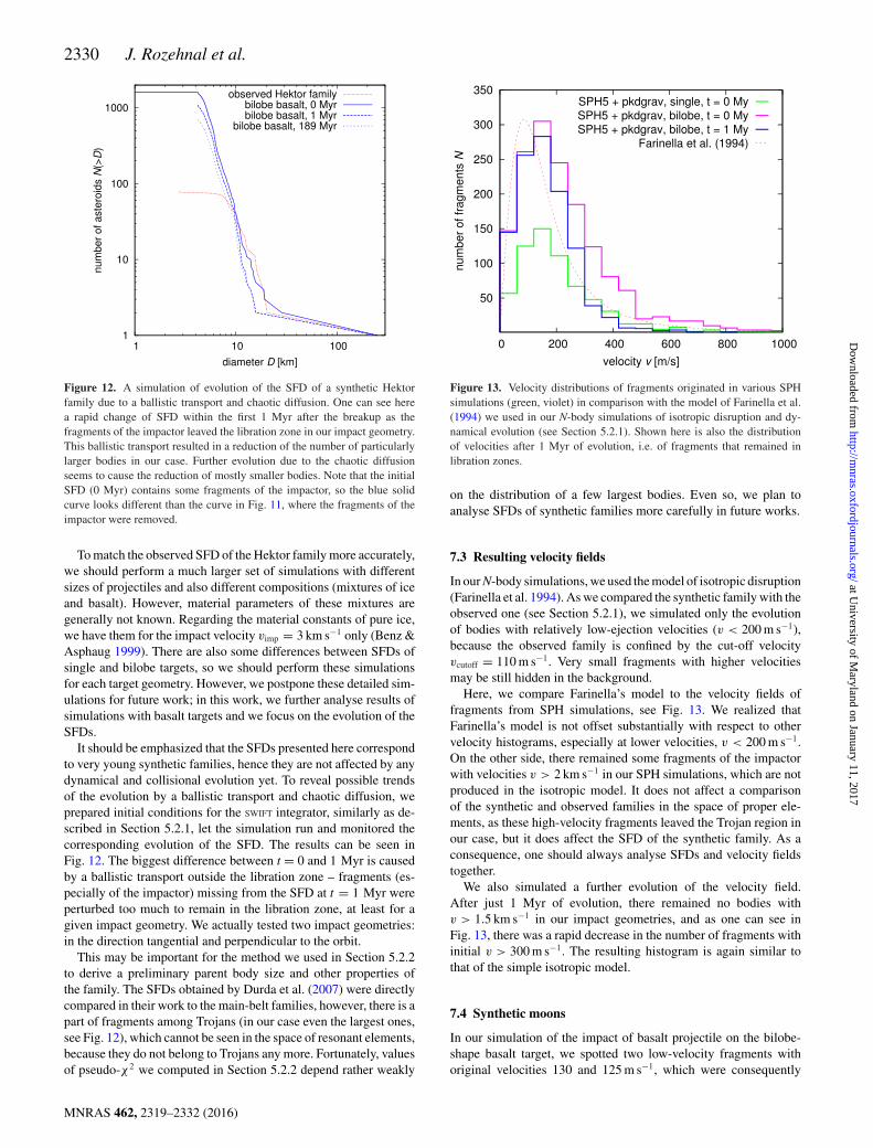
Figure 12. A simulation of evolution of the SFD of a synthetic Hektorfamily due to a ballistic transport and chaotic diffusion. One can see herea rapid change of SFD within the first 1 Myr after the breakup as thefragments of the impactor leaved the libration zone in our impact geometry.This ballistic transport resulted in a reduction of the number of particularlylarger bodies in our case. Further evolution due to the chaotic diffusionseems to cause the reduction of mostly smaller bodies. Note that the initialSFD (0 Myr) contains some fragments of the impactor, so the blue solidcurve looks different than the curve in Fig. 11, where the fragments of theimpactor were removed.

To match the observed SFD of the Hektor family more accurately,we should perform a much larger set of simulations with differentsizes of projectiles and also different compositions (mixtures of iceand basalt). However, material parameters of these mixtures aregenerally not known. Regarding the material constants of pure ice,we have them for the impact velocity vimp = 3 km s−1 only (Benz &Asphaug 1999). There are also some differences between SFDs ofsingle and bilobe targets, so we should perform these simulationsfor each target geometry. However, we postpone these detailed sim-ulations for future work; in this work, we further analyse results ofsimulations with basalt targets and we focus on the evolution of theSFDs.

It should be emphasized that the SFDs presented here correspondto very young synthetic families, hence they are not affected by anydynamical and collisional evolution yet. To reveal possible trendsof the evolution by a ballistic transport and chaotic diffusion, weprepared initial conditions for the SWIFT integrator, similarly as de-scribed in Section 5.2.1, let the simulation run and monitored thecorresponding evolution of the SFD. The results can be seen inFig. 12. The biggest difference between t = 0 and 1 Myr is causedby a ballistic transport outside the libration zone – fragments (es-pecially of the impactor) missing from the SFD at t = 1 Myr wereperturbed too much to remain in the libration zone, at least for agiven impact geometry. We actually tested two impact geometries:in the direction tangential and perpendicular to the orbit.

This may be important for the method we used in Section 5.2.2to derive a preliminary parent body size and other properties ofthe family. The SFDs obtained by Durda et al. (2007) were directlycompared in their work to the main-belt families, however, there is apart of fragments among Trojans (in our case even the largest ones,see Fig. 12), which cannot be seen in the space of resonant elements,because they do not belong to Trojans any more. Fortunately, valuesof pseudo-χ2 we computed in Section 5.2.2 depend rather weakly

Figure 13. Velocity distributions of fragments originated in various SPHsimulations (green, violet) in comparison with the model of Farinella et al.(1994) we used in our N-body simulations of isotropic disruption and dy-namical evolution (see Section 5.2.1). Shown here is also the distributionof velocities after 1 Myr of evolution, i.e. of fragments that remained inlibration zones.

on the distribution of a few largest bodies. Even so, we plan toanalyse SFDs of synthetic families more carefully in future works.

7.3 Resulting velocity fields

In our N-body simulations, we used the model of isotropic disruption(Farinella et al. 1994). As we compared the synthetic family with theobserved one (see Section 5.2.1), we simulated only the evolutionof bodies with relatively low-ejection velocities (v < 200 m s−1),because the observed family is confined by the cut-off velocityvcutoff = 110 m s−1. Very small fragments with higher velocitiesmay be still hidden in the background.

Here, we compare Farinella’s model to the velocity fields offragments from SPH simulations, see Fig. 13. We realized thatFarinella’s model is not offset substantially with respect to othervelocity histograms, especially at lower velocities, v < 200 m s−1.On the other side, there remained some fragments of the impactorwith velocities v > 2 km s−1 in our SPH simulations, which are notproduced in the isotropic model. It does not affect a comparisonof the synthetic and observed families in the space of proper ele-ments, as these high-velocity fragments leaved the Trojan region inour case, but it does affect the SFD of the synthetic family. As aconsequence, one should always analyse SFDs and velocity fieldstogether.

We also simulated a further evolution of the velocity field.After just 1 Myr of evolution, there remained no bodies withv > 1.5 km s−1 in our impact geometries, and as one can see inFig. 13, there was a rapid decrease in the number of fragments withinitial v > 300 m s−1. The resulting histogram is again similar tothat of the simple isotropic model.

7.4 Synthetic moons

In our simulation of the impact of basalt projectile on the bilobe-shape basalt target, we spotted two low-velocity fragments withoriginal velocities 130 and 125 m s−1, which were consequently

MNRAS 462, 2319–2332 (2016)

at University of M



ownloaded from



Table 4. A comparison of the sizes and the orbital parameters (i.e. semi-major axis a, eccentricity e and period P) of the observed moon of (624)Hektor as listed in Marchis et al. (2014), with the parameters of syntheticmoons SPH I and SPH II captured in our SPH simulation of impact on thebilobed target.

Desig. Diam. (km) a (km) e P (d)

Observed 12 ± 3 623.5 ± 10 0.31 ± 0.03 2.9651 ± 0.0003SPH I 2.2 715 0.82 1.2SPH II 2.7 370 0.64 0.4

captured as moons of the largest remnant. Their sizes and orbitalparameters are listed in Table 4.

These satellites were captured on orbits with high eccentricities(e = 0.82 and 0.64, respectively), which are much higher than theeccentricity of the observed moon determined by Marchis et al.(2014) (e = 0.31 ± 0.03). However, this could be partly caused bythe fact, that we handed the output of (gravity-free) SPH simulationsto the gravitational N-body code after first 100 s. Hence, fragmentsleaving the parent body could move freely without slowing downby gravity. More importantly, we do not account for any long-termdynamical evolution of the moons (e.g. by tides or binary YORP).

When compared to the observed satellite, the diameters of thesynthetic moons are several times smaller. This is not too surprising,given that the results for satellite formation are at the small endof what can be estimated with our techniques (median smoothinglength h = 2.3 km; satellite radius r � 1.2 km). The size of capturedfragments could also be dependent on impact conditions as differentimpact angles, impactor velocities and sizes (as is the case forscenarios of Moon formation) which we will analyse in detail in thefuture and study with more focused simulations.

8 C O N C L U S I O N S

In this paper, we updated the list of Trojans and their proper ele-ments, what allowed us to update parameters of Trojan families and

to discover a new one (namely 2001 UV209 in L5 population). Wefocused on the Hektor family, which seems the most interesting dueto the bilobed shape of the largest remnant with a small moon andalso its D-type taxonomical classification, which is unique amongthe collisional families observed so far.

At the current stage of knowledge, it seems to us there are no ma-jor inconsistencies among the observed number of Trojan familiesand their dynamical and collisional evolution, at least in the currentenvironment.

As usual, we ‘desperately’ need new observational data, namelyin the size range from 5 to 10 km, which would enable us to constrainthe ages of asteroid families on the basis of collisional modellingand to decide between two proposed ages of Hektor family, 1–4 Gyror 0.1–2.5 Gyr.

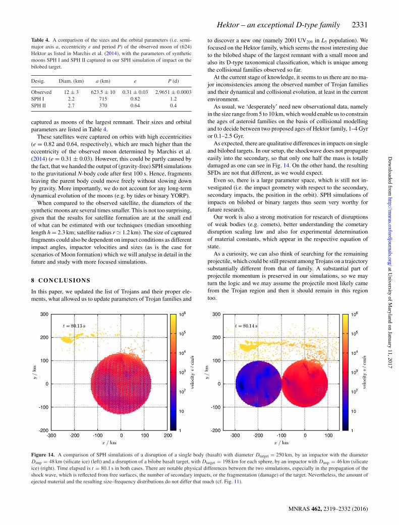
As expected, there are qualitative differences in impacts on singleand bilobed targets. In our setup, the shockwave does not propagateeasily into the secondary, so that only one half the mass is totallydamaged as one can see in Fig. 14. On the other hand, the resultingSFDs are not that different, as we would expect.

Even so, there is a large parameter space, which is still not in-vestigated (i.e. the impact geometry with respect to the secondary,secondary impacts, the position in the orbit). SPH simulations ofimpacts on bilobed or binary targets thus seem very worthy forfuture research.

Our work is also a strong motivation for research of disruptionsof weak bodies (e.g. comets), better understanding the cometarydisruption scaling law and also for experimental determinationof material constants, which appear in the respective equation ofstate.

As a curiosity, we can also think of searching for the remainingprojectile, which could be still present among Trojans on a trajectorysubstantially different from that of family. A substantial part ofprojectile momentum is preserved in our simulations, so we mayturn the logic and we may assume the projectile most likely camefrom the Trojan region and then it should remain in this regiontoo.

Figure 14. A comparison of SPH simulations of a disruption of a single body (basalt) with diameter Dtarget = 250 km, by an impactor with the diameterDimp = 48 km (silicate ice) (left) and a disruption of a bilobe basalt target, with Dtarget = 198 km for each sphere, by an impactor with Dimp = 46 km (silicateice) (right). Time elapsed is t = 80.1 s in both cases. There are notable physical differences between the two simulations, especially in the propagation of theshock wave, which is reflected from free surfaces, the number of secondary impacts, or the fragmentation (damage) of the target. Nevertheless, the amount ofejected material and the resulting size–frequency distributions do not differ that much (cf. Fig. 11).

MNRAS 462, 2319–2332 (2016)

at University of M



ownloaded from



AC K N OW L E D G E M E N T S

We thank Alessandro Morbidelli for his review which helped toimprove the final version of the paper.

The work of MB was supported by the grant no. P209/13/01308Sand that of JR by P209/15/04816S of the Czech Science Foundation(GA CR). We acknowledge the usage of computers of the StefanikObservatory, Prague.

R E F E R E N C E S

Benz W., Asphaug E., 1999, Icarus, 142, 5Bowell E., Virtanen J., Muinonen K., Boattini A., 2002, in Bottke W. F., Jr,

Cellino A., Paolicchi P., Binzel R. P., eds, Asteroids III. Univ. ArizonaPress, Tucson, p. 27

Broz M., Morbidelli A., 2013, Icarus, 223, 844Broz M., Rozehnal J., 2011, MNRAS, 414, 565Broz M. et al., 2013, AAP, 551, A117Carruba V., Nesvorny D., 2016, MNRAS, 457, 1332Chrenko O., Broz M., Nesvorny D., Tsiganis K., Skoulidou D. K., 2015,

MNRAS, 451, 2399Cruikshank D. P., Dalle Ore C. M., Roush T. L., Geballe T. R., Owen T. C.,

de Bergh C., Cash M. D., Hartmann W. K., 2001, Icarus, 153, 348Dell’Oro A., Marzari F., Paolicchi P., Dotto E., Vanzani V., 1998, A&A,

339, 272Dohnanyi J. S., 1969, J. Geophys Res., 74, 2531Durda D. D., Bottke W. F., Nesvorny D., Enke B. L., Merline W. J., Asphaug

E., Richardson D. C., 2007, Icarus, 186, 498Emery J. P., Cruikshank D. P., Van Cleve J., 2006, Icarus, 182, 496Emery J. P., Burr D. M., Cruikshank D. P., 2011, AJ, 114, 25Farinella P., Froeschle C., Gonczi R., 1994, in Milani A., Di Martino M.,

Cellino A., eds., Asteroids, Comets, Meteors 1993. Kluwer AcademicPublishers, Dordrecht, p. 205

Goldreich P., Lithwick Y., Sari R., 2004, ApJ, 614, 497Grav T. et al., 2011, ApJ, 742, 40Grav T., Mainzer A. K., Bauer J., Masiero J. R., Nugent C. R., 2012, ApJ,

759, 49Ivezic Z., Juric M., Lupton R. H., Tabachnik S., Quinn T., 2002, in Tyson

J. A., Wolff S., eds, Proc. SPIE Conf. Ser. Vol. 4836, Survey and OtherTelescope Technologies and Discoveries. Kluwer, Dordrecht, p. 98

Laskar J., Robutel P., 2001, Celest. Mech. Dyn. Astron., 80, 39Levison H. F., Duncan M., 1994, Icarus, 108, 18Levison H. F., Bottke W. F., Gounelle M., Morbidelli A., Nesvorny D.,

Tsiganis K., 2009, Nature, 460, 364Lyra W., Johansen A., Klahr H., Piskunov N., 2009, A&A, 493, 1125Mainzer A. et al., 2011, ApJ, 741, 90Marchis F. et al., 2014, ApJ, 783, L37Morbidelli A., Levison H. F., Tsiganis K., Gomes R., 2005, Nature, 435,

462Morbidelli A., Bottke W. F., Nesvorny D., Levison H. F., 2009, Icarus, 204,

558Morbidelli A., Brasser R., Gomes R., Levison H. F., Tsiganis K., 2010, AJ,

140, 1391Nesvorny D., Vokrouhlicky D., Morbidelli A., 2013, ApJ, 768, 45Nesvorny D., Broz M., Carruba V., 2015, in Michel P., DeMeo F. E., Bottke

W. F., eds, Asteroids IV. Arizona Univ. Press, Tucson, p. 297Richardson D. C., Quinn T., Stadel J., Lake G., 2000, Icarus, 143, 45Tillotson E, 1962, Nature, 195, 763Usui F. et al., 2011, PASJ, 63, 1117Vinogradova T. A., 2015, MNRAS, 454, 2436Zappala V., Cellino A., Farinella P., Milani A., 1994, AJ, 107, 772

This paper has been typeset from a TEX/LATEX file prepared by the author.

MNRAS 462, 2319–2332 (2016)

at University of M



ownloaded from


hektor – an exceptional d-type family among jovian trojansdcr/reprints/rozehnal_mnras... ·...

Documents