herded gibbs sampling - luke bornn · 2016-04-18 · herded gibbs is shown to outperform gibbs in...
TRANSCRIPT

Journal of Machine Learning Research 17 (2016) 1-29 Submitted 6/13; Revised 10/14; Published 3/16
Herded Gibbs Sampling
Yutian Chen [email protected] Pancras Square, Kings Cross, London, N1C 4AG, United Kingdom
Luke Bornn [email protected] & Actuarial Science, Simon Fraser University, 8888 University Drive, Burnaby, BC,V5A1S6, Canada
Nando de Freitas [email protected] Pancras Square, Kings Cross, London, N1C 4AG, United Kingdom
Mareija Eskelin [email protected] of Computer Science, University of British Columbia, 2366 Main Mall, Vancouver, BC,V6T1Z4, Canada
Jing Fang [email protected] Facebook Way, Menlo Park, CA, 94025, United States
Max Welling [email protected]
Informatics Institute, Science Park 904, Postbus 94323, 1090 GH, Amsterdam, Netherlands
Editor: Aaron Courville, Rob Fergus, and Christopher Manning
Abstract
The Gibbs sampler is one of the most popular algorithms for inference in statistical models.In this paper, we introduce a herding variant of this algorithm, called herded Gibbs, thatis entirely deterministic. We prove that herded Gibbs has an O(1/T ) convergence rate formodels with independent variables and for fully connected probabilistic graphical models.Herded Gibbs is shown to outperform Gibbs in the tasks of image denoising with MRFsand named entity recognition with CRFs. However, the convergence for herded Gibbs forsparsely connected probabilistic graphical models is still an open problem.
Keywords: Gibbs sampling, herding, deterministic sampling
1. Introduction
Over the last 60 years, we have witnessed great progress in the design of randomized sam-pling algorithms; see for example Liu (2001); Doucet et al. (2001); Andrieu et al. (2003);Robert and Casella (2004) and the references therein. In contrast, the design of determin-istic algorithms for “sampling” from distributions is still in its inception (Chen et al., 2010;Holroyd and Propp, 2010; Chen et al., 2011; Murray and Elliott, 2012). There are, however,many important reasons for pursuing this line of attack on the problem. From a theoret-ical perspective, this is a well defined mathematical challenge whose solution might haveimportant consequences. It also brings us closer to reconciling the fact that we typicallyuse pseudo-random number generators to run Monte Carlo algorithms on classical, VonNeumann architecture, computers. Moreover, the theory for some of the recently proposeddeterministic sampling algorithms has taught us that they can achieve O(1/T ) convergence
c©2016 Yutian Chen, Luke Bornn, Nando de Freitas, Mareija Eskelin, Jing Fang, and Max Welling.

Chen et al.
rates (Chen et al., 2010; Holroyd and Propp, 2010), which are much faster than the standardMonte Carlo rates of O(1/
√T ) for computing ergodic averages. From a practical perspec-
tive, the design of deterministic sampling algorithms creates an opportunity for researchersto apply a great body of knowledge on optimization to the problem of sampling; see forexample Bach et al. (2012) for an early example of this.
The domain of application of currently existing deterministic sampling algorithms isstill very narrow. Importantly, the only available deterministic tool for sampling fromunnormalized multivariate probability distributions is the Markov Chain Quasi-Monte Carlomethod (Chen et al., 2011), but there is no theoretical result to show a better convergencerate than a standard MCMC method yet. This is very limiting because the problem ofsampling from unnormalized distributions is at the heart of the field of Bayesian inferenceand the probabilistic programming approach to artificial intelligence (Lunn et al., 2000;Carbonetto et al., 2005; Milch and Russell, 2006; Goodman et al., 2008). At the same time,despite great progress in Monte Carlo simulation, the celebrated Gibbs sampler continues tobe one of the most widely-used algorithms. For example, it is the inference engine behindpopular statistics packages (Lunn et al., 2000), several tools for text analysis (Porteouset al., 2008), and Boltzmann machines (Ackley et al., 1985; Hinton and Salakhutdinov,2006). The popularity of Gibbs stems from its generality and simplicity of implementation.
Without any doubt, it would be remarkable if we could design generic deterministicGibbs samplers with fast (theoretical and empirical) rates of convergence. In this paper,we take steps toward achieving this goal by capitalizing on a recent idea for deterministicsimulation known as herding. Herding (Welling, 2009a,b; Gelfand et al., 2010) is a deter-ministic procedure for generating samples x ∈ X ⊆ Rn, such that the empirical moments µof the data are matched. The herding procedure, at iteration t, is as follows:
x(t) = arg maxx∈X
〈w(t−1),φ(x)〉,
w(t) = w(t−1) + µ− φ(x(t)), (1)
where φ : X → H is a feature map (statistic) from X to a Hilbert spaceH with inner product〈·, ·〉, w ∈ H is the vector of parameters, and µ ∈ H is the moment vector (expected valueof φ over the data) that we want to match. If we choose normalized features by making‖φ(x)‖ constant for all x, then the update to generate samples x(t) for t = 1, 2, . . . , T inEquation 1 is equivalent to minimizing the objective
J(x1, . . . ,xT ) =
∥∥∥∥∥µ− 1
T
T∑t=1
φ(x(t))
∥∥∥∥∥2
, (2)
where T may have no prior known value and ‖ · ‖ =√〈·, ·〉 is the naturally defined norm
based upon the inner product of the space H (Chen et al., 2010; Bach et al., 2012).Herding can be used to produce samples from normalized probability distributions.
This is done as follows. Let µ denote a discrete, normalized probability distribution, withµi ∈ [0, 1] and
∑ni=1 µi = 1. A natural feature in this case is the vector φ(x) that has
all entries equal to zero, except for the entry at the position indicated by x. For instance,if x = 2 and n = 5, we have φ(x) = (0, 1, 0, 0, 0)T . Hence, µ = T−1
∑Tt=1φ(x(t)) is
an empirical estimate of the distribution. In this case, one step of the herding algorithm
2
Herded Gibbs Sampling
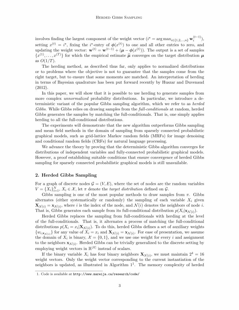
involves finding the largest component of the weight vector (i? = arg maxi∈{1,2,...,n}w(t−1)i ),
setting x(t) = i?, fixing the i?-entry of φ(x(t)) to one and all other entries to zero, andupdating the weight vector: w(t) = w(t−1) + (µ− φ(x(t))). The output is a set of samples{x(1), . . . , x(T )} for which the empirical estimate µ converges on the target distribution µas O(1/T ).
The herding method, as described thus far, only applies to normalized distributionsor to problems where the objective is not to guarantee that the samples come from theright target, but to ensure that some moments are matched. An interpretation of herdingin terms of Bayesian quadrature has been put forward recently by Huszar and Duvenaud(2012).
In this paper, we will show that it is possible to use herding to generate samples frommore complex unnormalized probability distributions. In particular, we introduce a de-terministic variant of the popular Gibbs sampling algorithm, which we refer to as herdedGibbs. While Gibbs relies on drawing samples from the full-conditionals at random, herdedGibbs generates the samples by matching the full-conditionals. That is, one simply appliesherding to all the full-conditional distributions.
The experiments will demonstrate that the new algorithm outperforms Gibbs samplingand mean field methods in the domain of sampling from sparsely connected probabilisticgraphical models, such as grid-lattice Markov random fields (MRFs) for image denoisingand conditional random fields (CRFs) for natural language processing.
We advance the theory by proving that the deterministic Gibbs algorithm converges fordistributions of independent variables and fully-connected probabilistic graphical models.However, a proof establishing suitable conditions that ensure convergence of herded Gibbssampling for sparsely connected probabilistic graphical models is still unavailable.
2. Herded Gibbs Sampling
For a graph of discrete nodes G = (V,E), where the set of nodes are the random variablesV = {Xi}Ni=1, Xi ∈ X , let π denote the target distribution defined on G.
Gibbs sampling is one of the most popular methods to draw samples from π. Gibbsalternates (either systematically or randomly) the sampling of each variable Xi givenXN (i) = xN (i), where i is the index of the node, and N (i) denotes the neighbors of node i.That is, Gibbs generates each sample from its full-conditional distribution p(Xi|xN (i)).
Herded Gibbs replaces the sampling from full-conditionals with herding at the levelof the full-conditionals. That is, it alternates a process of matching the full-conditionaldistributions p(Xi = xi|XN (i)). To do this, herded Gibbs defines a set of auxiliary weights{wi,xN (i)
} for any value of Xi = xi and XN (i) = xN (i). For ease of presentation, we assumethe domain of Xi is binary, X = {0, 1}, and we use one weight for every i and assignmentto the neighbors xN (i). Herded Gibbs can be trivially generalized to the discrete setting by
employing weight vectors in R|X | instead of scalars.
If the binary variable Xi has four binary neighbors XN (i), we must maintain 24 = 16weight vectors. Only the weight vector corresponding to the current instantiation of theneighbors is updated, as illustrated in Algorithm 11. The memory complexity of herded
1. Code is available at http://www.mareija.ca/research/code/
3

Chen et al.
Algorithm 1 Herded Gibbs Sampling
Input: T .
Step 1: Set t = 0. Initialize X(0) in the support of π and w(0)i,xN (i)
in (π(Xi = 1|xN (i)) −1, π(Xi = 1|xN (i))).for t = 1→ T do
Step 2: Pick a node i according to some policy. Denote w = w(t−1)i,x
(t−1)N (i)
.
Step 3: If w > 0, set x(t)i = 1, otherwise set x
(t)i = 0.
Step 4: Update weight w(t)
i,x(t)N (i)
= w(t−1)i,x
(t−1)N (i)
+ π(Xi = 1|x(t−1)N (i) )− x(t)i .
Step 5: Keep the values of all the other nodes x(t)j = x
(t−1)j ,∀j 6= i and all the other
weights w(t)j,xN (j)
= w(t−1)j,xN (j)
,∀j 6= i or xN (j) 6= x(t−1)N (i) .
end forOutput: x(1), . . . ,x(T )
Gibbs is exponential in the maximum node degree. Note the algorithm is a deterministicMarkov process with state (X,W).
The initialization in the first step of Algorithm 1 guarantees that X(t) always remainsin the support of π with the reason to be explained in Section 3.1. For a deterministic scanpolicy in step 2, we take the value of variables x(tN), t ∈ N as a sample sequence. Throughoutthe paper all experiments employ a fixed variable traversal for sample generation. We callone such traversal of the variables a sweep.
3. Analysis
As herded Gibbs sampling is a deterministic algorithm, the probability distribution of thesample at any step t is a single point mass and there is no stationary distribution of states.Instead, we examine the average of the sample states over time and hypothesize that itconverges to the joint distribution, our target distribution, π. To make the treatmentprecise, we need the following definition:
Definition 1 For a graph of discrete nodes G = (V,E), where the set of nodes V = {Xi}Ni=1,
Xi ∈ X , P(τ)T is the empirical estimate of the joint distribution obtained by averaging over
T samples acquired from G. P(τ)T is derived from T samples, collected at the end of every
sweep over N variables, starting from the τ th sweep:
P(τ)T (X = x) =
1
T
τ+T−1∑k=τ
I(X(kN) = x). (3)
The definition of P(τ)T is illustrated in Figure 1. Our goal is to prove that the limiting
average sample distribution over time converges to the target distribution π. Specifically,we want to show the following:
limT→∞
P(τ)T (x) = π(x), ∀τ ≥ 0. (4)
4

Herded Gibbs Sampling
Figure 1: Sample distribution over T sweeps. Each node refers to the joint state at the endof one sweep.
If this holds, we also want to know what the convergence rate is.
3.1 Single Variable Models
We begin the theoretical analysis with a graph of one binary variable. For this graph, thereis only one weight w and herded Gibbs is equivalent to the standard herding algorithm.Denote π(X = 1) as π for notational simplicity. The sequence of X is determined by thedynamics of w (shown in Figure 2a):
w(t) = w(t−1) + π − I(w(t−1) > 0), X(t) =
{1 if w(t−1) > 00 otherwise
. (5)
The following lemma shows that (π − 1, π] is the invariant interval of the dynamics.
Lemma 1 If w is the weight of the herding dynamics of a single binary variable X withprobability P (X = 1) = π, and w(s) ∈ (π − 1, π] at some step s ≥ 0, then w(t) ∈ (π −1, π], ∀t ≥ s. Moreover, for T ∈ N, we have:
s+T∑t=s+1
I[X(t) = 1] ∈ [Tπ − 1, Tπ + 1], (6)
s+T∑t=s+1
I[X(t) = 0] ∈ [T (1− π)− 1, T (1− π) + 1]. (7)
See the proof in Appendix A. It follows immediately that the state X = 1 is visited at afrequency close to π with an error:
|P (τ)T (X = 1)− π| ≤ 1
T. (8)
This is known as the fast moment matching property in Welling (2009a,b); Gelfand et al.(2010). When w is outside the invariant interval, it is easy to observe that w will moveinto it monotonically at a linear speed in a transient period. So we will always consider aninitialization of w ∈ (π − 1, π] from now on.
Another immediate consequence of Lemma 1 is that the initialization in Algorithm 1ensures that X(t) always remain in the support of π. That is because when we consider
5

Chen et al.
the set of iterations that involves a particular weight wi,xN (i), the dynamics of that weight
is equivalent to that of a single variable model with a probability π(Xi = 1|xN (i)). If a
joint state X is going to move outside the support at some iteration t, from e. g. x(t−1) =(xi = 0,x−i) to x(t) = (xi = 1,x−i) where x−i denotes all the other variables but xi, then
the corresponding weight w(t−1)i,xN (i)
must be positive according to the algorithm. However,
the conditional probability π(Xi = 1|xN (i)) = 0 because π(x(t−1)) > 0 and π(x(t)) = 0.
Following Lemma 1 the weight w(t−1)i,xN (i)
∈ (−1, 0], leading to a contradiction. The same
argument applies when X tries to move from x(t−1) = (xi = 1,x−i) to x(t) = (xi = 0,x−i).Therefore, once initialized inside the support, the samples of Algorithm 1 will remain in thesupport for any t > 0.
It will be useful for the next section to introduce an equivalent representation of theweight dynamics by taking a one-to-one mapping w ← w mod 1 (we define 1 mod 1 = 1)with a little abuse of the symbol w. We think of the new variable w as updated by aconstant translation vector in a circular unit interval (0, 1] as shown in Figure 2b. That is,
w(t) = (w(t−1) + π) mod 1, X(t) =
{1 if w(t−1) < π0 otherwise
. (9)
(a) Representation in Equation 5.
(b) Equivalent representation.
Figure 2: Herding dynamics for a singlevariable. Black arrows show thetrajectory of w(t) for 2 iterations.
Figure 3: Herding dynamics for two inde-pendent variables in the equiva-lent representation.
3.2 Empty Graphs
The analysis of herded Gibbs for empty graphs is a natural extension of that for singlevariables. In an empty graph, all the variables are independent of each other and herdedGibbs reduces to runningN one-variable chains in parallel. Denote the marginal distributionπi := π(Xi = 1).
Examples of failing convergence in the presence of rational ratios between the πis wereobserved in Bach et al. (2012). There the need for further theoretical research on this matter
6

Herded Gibbs Sampling
was pointed out. The following theorem provides a sufficient condition for convergence inthe restricted domain of empty graphs.
Theorem 2 For an empty graph, when herded Gibbs has a fixed scanning order, and
{1, π1, . . . , πN} are rationally independent, the empirical distribution P(τ)T converges to the
target distribution π as T →∞ for any τ ≥ 0.
A set of n real numbers, x1, x2, . . . , xn, is said to be rationally independent if for any set ofrational numbers, a1, a2, . . . , an, we have
∑ni=1 aixi = 0⇔ ai = 0, ∀1 ≤ i ≤ n.
Proof For an empty graph of N independent vertices, the dynamics of the weight vectorw after one sweep over all variables are equivalent to a constant translation mapping in anN -dimensional circular unit space (0, 1]N , as shown in Figure 3:
w(t) = (w(t−1) + π) mod 1
= (w(0) + tπ) mod 1, x(t)i =
{1 if w
(t−1)i < πi
0 otherwise, ∀1 ≤ i ≤ N. (10)
The Kronecker-Weyl theorem (Weyl, 1916) states that the sequence w(t) = tπ mod 1, t ∈Z+ is equidistributed (or uniformly distributed) on (0, 1]N if and only if (1, π1, . . . , πN )is rationally independent. Intuitively, when (1, π1, . . . , πN ) is rationally independent, thetrajectory of w(t) can not form a closed loop in the circular unit space and will therebycover the entire space uniformly.
Since we can define a one-to-one volume preserving transformation between w(t) and w(t)
as (w(t) + w(0)) mod 1 = w(t), the sequence of weights {w(t)} is also uniformly distributedin (0, 1]N .
Now define the mapping from a state value xi to an interval of wi as
Ai(x) =
{(0, πi] if x = 1(πi, 1] if x = 0
(11)
and let |Ai| be its measure. We obtain the limiting distribution of the joint state as
limT→∞
P(τ)T (X = x) = lim
T→∞
1
T
T∑t=1
I
[w(t−1) ∈
N∏i=1
Ai(xi)
]
=N∏i=1
|Ai(xi)| =N∏i=1
π(Xi = xi) = π(X = x). (12)
The rational independence condition in the application of the Kronecker-Weyl theoremensures that the probabilistic independence between different variables will be respected bythe herding dynamics. When the condition fails, the convergence of joint distribution is notguaranteed but the marginal distribution of each variables will still converge to their targetdistribution because the N one-variable chains run independently from each other.
7

Chen et al.
3.3 Fully-Connected Graphs
When herded Gibbs is applied to fully-connected (complete) graphs, convergence is guar-anteed even with rationally dependent conditional probabilities. In fact, herded Gibbsconverges to the target joint distribution at a rate of O(1/T ) with a O(log(T )) burn-inperiod. This statement is formalized in Theorem 3 and a corollary when we ignore theburn-in period, with proofs provided respectively in Appendix B.4 and B.5.
Theorem 3 For a fully-connected graph, when herded Gibbs has a fixed scanning orderand a Dobrushin coefficient of the corresponding Gibbs sampler η < 1, there exist constantsl > 0, and B > 0 such that
dv(P(τ)T − π) ≤ λ
T, ∀T ≥ T ∗, τ > τ∗(T ), (13)
where λ = 2N(1+η)l(1−η) , T ∗ = 2B
l , τ∗(T ) = log 21+η
((1−η)lT
4N
), and dv(δπ) := 1
2 ||δπ||1.
Corollary 4 When the conditions of Theorem 3 hold, and we start collecting samples atthe end of every sweep from the beginning, that is setting τ = 0, the error of the sampledistribution is bounded by:
dv(P(τ=0)T − π) ≤ λ+ τ∗(T )
T= O(
log(T )
T), ∀T ≥ T ∗ + τ∗(T ∗). (14)
The Dobrushin ergodic coefficient (Bremaud, 1999) measures the geometric convergencerate of a Markov chain. The constant l in the convergence rate can be interpreted as a lowerbound of the transition probability between any pair of states in the support of the targetdistribution. For a strictly positive distribution, the constants l and B are
l = πNmin, B = πNmin +1− (2πmin)N
1− 2πmin. (15)
where πmin is the minimal conditional probability πmin = min1≤i≤N,x−i π(xi|x−i). We referthe readers to Equation 34 in Proposition 5 in the appendix for a general distribution. Noticethat l has an exponential term, with N in the exponent, leading to an exponentially largeconstant. This is unavoidable for any sampling algorithm when considering the convergenceto a joint distribution with 2N states. As for the marginal distributions, it is obvious thatthe convergence rate of herded Gibbs is also O(1/T ) because marginal probabilities arelinear functions of the joint distribution. In fact, we observe very rapid convergence resultsfor the marginals in practice, so stronger theoretical results about the convergence of themarginal distributions seem plausible.
The proof proceeds by first bounding the discrepancy between the chain of empirical
estimates of the joint obtained by averaging over T herded Gibbs samples, {P (s)T }, s ≥ τ ,
and a Gibbs chain initialized at P(τ)T . After one sweep over N variables, this discrepancy is
bounded above by 2N/lT .
The Gibbs chain has geometric convergence to π and the distance between the Gibbs
and herded Gibbs chains decreases as O(1/T ). When the distance between P(τ)T and π is
8

Herded Gibbs Sampling
sufficiently large, the geometric convergence rate to π dominates the discrepancy of herded
Gibbs and thus we infer that P(τ)T converges to a neighborhood of π geometrically in time
τ for a fixed T . To round-off the proof, we must find a limiting value for τ . The proofconcludes with an O(log(T )) burn-in for τ .
When there exist conditional independencies in a distribution, we can still apply herdedGibbs with a fully connected graph and treat all the other variables as the Markov blanketof the variable to be sampled. Theorem 3 and its corollary still apply. Alternatively, wecan apply herded Gibbs on a more compact representation with an incomplete graph. Itrequires less memory to run herded Gibbs because the number of weights depends expo-nentially on the neighborhood size. However, for a generic graph we have no mathematicalguarantees for the convergence rate of herded Gibbs. In fact, one can easily construct syn-thetic examples for which herded Gibbs does not seem to converge to the true marginalsand joint distribution. For the examples covered by our theorems and for examples withreal data, herded Gibbs demonstrates good behaviour. The exact conditions under whichherded Gibbs converges for sparsely connected graphs are still unknown.
4. Experiments
We illustrate the performance of herded Gibbs with two synthetic examples and two realexperiments for image denoising and natural language processing respectively.
4.1 Simple Complete Graph
We begin with an illustration of how herded Gibbs substantially outperforms Gibbs anda deterministic Gibbs sampler based on MCQMC on a simple complete graph. The MC-QMC algorithm replaces the random number generator of the regular Gibbs sampler witha completely uniformly distributed (CUD) sequence (Chen et al., 2011). We consider afully-connected model of two variables, X1 and X2, as shown in Figure 4; the joint distri-bution of these variables is shown in Table 1. We run each sampler for 2.6× 10⁵ iterations.We use a small linear feedback shift registers (LFSR) described in (Chen et al., 2012) togenerate the CUD sequence and choose the size of the LFSR so that the entire period ofthe sequence will be used for one run of the Markov chain. Both Gibbs and MCQMC-basedGibbs are run 100 times with different random seeds to assess their average performance.Herded Gibbs is run only once because different initialization does not show noticeable dif-ference in its performance. Figure 5 shows the marginal distribution P (X1 = 1) and thejoint distribution approximated by all the algorithms for different ε. As ε decreases, allthe approaches require more iterations to converge, but herded Gibbs clearly outperformsthe other two algorithms. Figure 5c also shows that herding does indeed exhibit a linearconvergence rate. MCQMC-based Gibbs does not show any improvement on the error ofthe sample distribution compared to the standard Gibbs.
4.2 Simple Incomplete Graph
We also illustrate a simple counterexample where the sample distribution of herded Gibbsdoes not converge to the target distribution when the graph is incomplete. Figure 7 showsa four-variable graphical model with two missing edges, X1 − X4, X2 − X3. The unary
9
Chen et al.
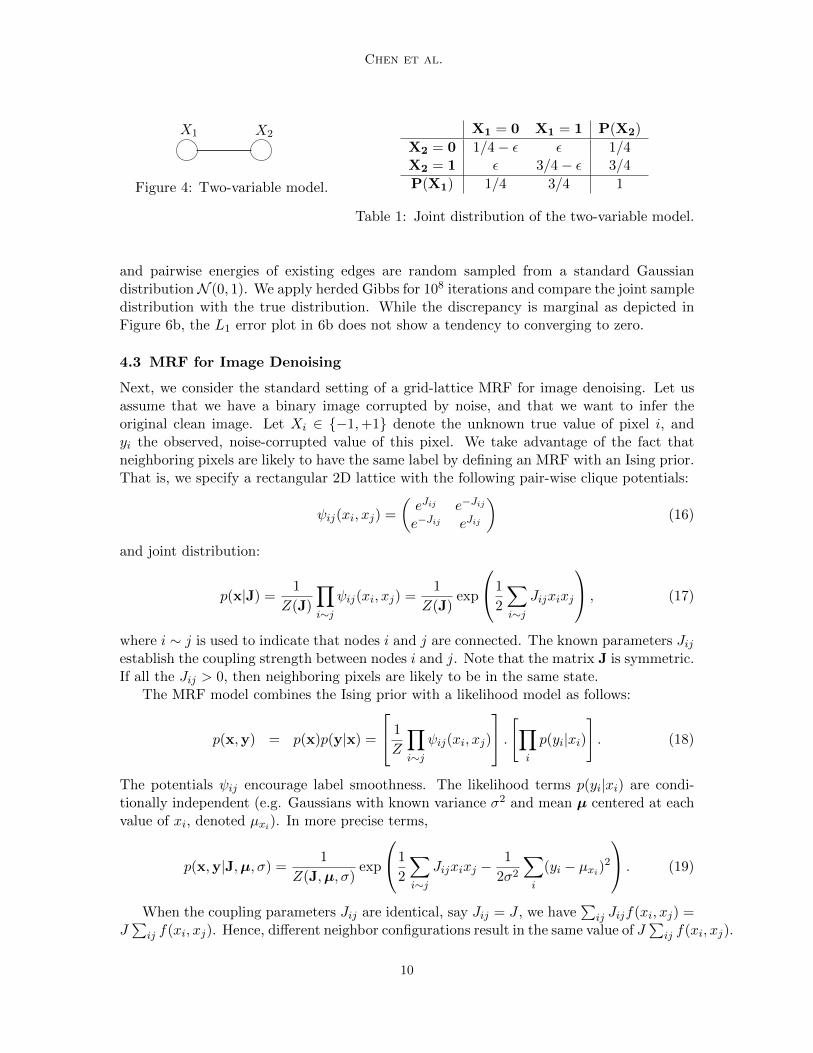
X1 X2
Figure 4: Two-variable model.
X1 = 0 X1 = 1 P(X2)
X2 = 0 1/4− ε ε 1/4X2 = 1 ε 3/4− ε 3/4
P(X1) 1/4 3/4 1
Table 1: Joint distribution of the two-variable model.
and pairwise energies of existing edges are random sampled from a standard GaussiandistributionN (0, 1). We apply herded Gibbs for 108 iterations and compare the joint sampledistribution with the true distribution. While the discrepancy is marginal as depicted inFigure 6b, the L1 error plot in 6b does not show a tendency to converging to zero.
4.3 MRF for Image Denoising
Next, we consider the standard setting of a grid-lattice MRF for image denoising. Let usassume that we have a binary image corrupted by noise, and that we want to infer theoriginal clean image. Let Xi ∈ {−1,+1} denote the unknown true value of pixel i, andyi the observed, noise-corrupted value of this pixel. We take advantage of the fact thatneighboring pixels are likely to have the same label by defining an MRF with an Ising prior.That is, we specify a rectangular 2D lattice with the following pair-wise clique potentials:
ψij(xi, xj) =
(eJij e−Jij
e−Jij eJij
)(16)
and joint distribution:
p(x|J) =1
Z(J)
∏i∼j
ψij(xi, xj) =1
Z(J)exp
1
2
∑i∼j
Jijxixj
, (17)
where i ∼ j is used to indicate that nodes i and j are connected. The known parameters Jijestablish the coupling strength between nodes i and j. Note that the matrix J is symmetric.If all the Jij > 0, then neighboring pixels are likely to be in the same state.
The MRF model combines the Ising prior with a likelihood model as follows:
p(x,y) = p(x)p(y|x) =
1
Z
∏i∼j
ψij(xi, xj)
.[∏i
p(yi|xi)
]. (18)
The potentials ψij encourage label smoothness. The likelihood terms p(yi|xi) are condi-tionally independent (e.g. Gaussians with known variance σ2 and mean µ centered at eachvalue of xi, denoted µxi). In more precise terms,
p(x,y|J,µ, σ) =1
Z(J,µ, σ)exp
1
2
∑i∼j
Jijxixj −1
2σ2
∑i
(yi − µxi)2 . (19)
When the coupling parameters Jij are identical, say Jij = J , we have∑
ij Jijf(xi, xj) =J∑
ij f(xi, xj). Hence, different neighbor configurations result in the same value of J∑
ij f(xi, xj).
10

Herded Gibbs Sampling
(a) Approximate marginals.
(b) Log-log plot of the L1 error of the joint distribution.
(c) Inverse of the L1 error of the joint distribution.
Figure 5: Approximating a marginal (a) and joint (b, c) distribution with Gibbs (blue),MCQMC-based Gibbs (green) and herded Gibbs (red) for an MRF of two vari-ables, constructed so as to make the move from state (0, 0) to (1, 1) progressivelymore difficult as ε decreases. The four columns, from left to right, are for ε = 0.1,ε = 0.01, ε = 0.001 and ε = 0.0001. Table 1 provides the joint distributionfor these variables. The shaded areas for Gibbs and MCQMC-based Gibbs cor-respond to 25%-75% quantile of 100 runs. Rows (b) and (c) illustrate that theempirical convergence rate of herded Gibbs matches the expected theoretical rate.As the error of herded Gibbs in (b) and (c) frequently drops to extremely smallvalues for some iterations and jumps back, we plot the upper-bound (envelope)of the error for herded Gibbs defined as et = maxτ≥t eτ to remove the oscillatingbehavior for a better visualization.
11

Chen et al.
x1 x2
x3 x4(a)
1 2 3 4 5 6 7 8 9 10 11 12 13 14 15 160
0.05
0.1
0.15
0.2
0.25
0.3
0.35
Joint State
Pro
babili
ty
Sample Distribution
Ground Truth
(b)
104
105
106
107
108
10−3
10−2
10−1
Iterations
L1 E
rror
of Join
t P
robabili
ty
(c)
Figure 7: Four-variable model represented as an incomplete graph. (a): Graphical Model.(b): Joint distribution of samples from herded Gibbs vs. the ground truth. (c):Log-log plot of the L1 error of the joint sample distribution.
If we store the conditionals for configurations with the same sum together, we only need tostore as many conditionals as different possible values that the sum could take. This enablesus to develop a shared version of herded Gibbs that is more memory efficient where we onlymaintain and update weights for distinct states of the Markov blanket of each variable. Theshared version of herded Gibbs also exhibits a different dynamics as the standard versionas shown in the following result, and the convergence property of this algorithm remains anopen problem.
In this exemplary image denoising experiment, noisy versions of the binary image, de-picted in Figure 8 (left), were created through the addition of Gaussian noise, with varyingσ. Figure 8 (right) shows a corrupted image with σ = 4. The L2 reconstruction errorsas a function of the number of iterations, for this example, are shown in Figure 9. Theplot compares the herded Gibbs method against Gibbs and two versions of mean field withdifferent damping factors (Murphy, 2012). The results demonstrate that the herded Gibbstechniques are among the best methods for solving this task.
A comparison for different values σ is presented in Table 2. As expected mean field doeswell in the low-noise scenario, but the performance of the shared version of herded Gibbsas the noise increases is significantly better.
4.4 CRF for Named Entity Recognition
Named entity recognition (NER) involves the identification of entities, such as people andlocations, within a text sample. A conditional random field (CRF) for NER models therelationship between entity labels and sentences with a conditional probability distribution:P (X|Y, θ), where X is a labeling, Y is a sentence, and θ is a vector of coupling parameters.The parameters, θ, are feature weights and model relationships between variables Xi andYj or Xi and Xj . A chain CRF only employs relationships between adjacent variables,whereas a skip-chain CRF can employ relationships between variables where subscripts iand j differ dramatically. Skip-chain CRFs are important in language tasks, such as NER
12

Herded Gibbs Sampling
Figure 8: Original image (left) and its corrupted version (right), with noise parameter σ = 4.
Figure 9: Reconstruction errors for the image denoising task. The results are averagedacross 10 corrupted images with Gaussian noise N (0, 16). The error bars cor-respond to one standard deviation. Mean field requires the specification of thedamping factor D.
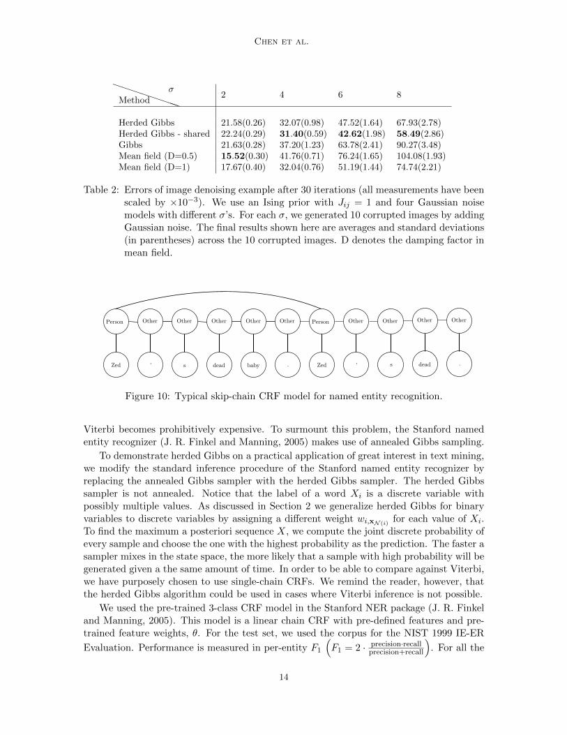
and semantic role labeling, because they allow us to model long dependencies in a streamof words, see Figure 10.
Once the parameters have been learned, the CRF can be used for inference; a labeling forsome sentence Y is found by maximizing the above probability. Inference for CRF modelsin the NER domain is typically carried out with the Viterbi algorithm. However, if we wantto accommodate long term dependencies, thus resulting in the so called skip-chain CRFs,
13
Chen et al.
PPPPPPPPMethodσ
2 4 6 8
Herded Gibbs 21.58(0.26) 32.07(0.98) 47.52(1.64) 67.93(2.78)Herded Gibbs - shared 22.24(0.29) 31.40(0.59) 42.62(1.98) 58.49(2.86)Gibbs 21.63(0.28) 37.20(1.23) 63.78(2.41) 90.27(3.48)Mean field (D=0.5) 15.52(0.30) 41.76(0.71) 76.24(1.65) 104.08(1.93)Mean field (D=1) 17.67(0.40) 32.04(0.76) 51.19(1.44) 74.74(2.21)
Table 2: Errors of image denoising example after 30 iterations (all measurements have beenscaled by ×10−3). We use an Ising prior with Jij = 1 and four Gaussian noisemodels with different σ’s. For each σ, we generated 10 corrupted images by addingGaussian noise. The final results shown here are averages and standard deviations(in parentheses) across the 10 corrupted images. D denotes the damping factor inmean field.
Other
’
Person
Zed
Other
s
Other
.
Other
’
Person
Zed
Other
s
Other
dead
Other
.
Other
dead
Other
baby
Figure 10: Typical skip-chain CRF model for named entity recognition.
Viterbi becomes prohibitively expensive. To surmount this problem, the Stanford namedentity recognizer (J. R. Finkel and Manning, 2005) makes use of annealed Gibbs sampling.
To demonstrate herded Gibbs on a practical application of great interest in text mining,we modify the standard inference procedure of the Stanford named entity recognizer byreplacing the annealed Gibbs sampler with the herded Gibbs sampler. The herded Gibbssampler is not annealed. Notice that the label of a word Xi is a discrete variable withpossibly multiple values. As discussed in Section 2 we generalize herded Gibbs for binaryvariables to discrete variables by assigning a different weight wi,xN (i)
for each value of Xi.To find the maximum a posteriori sequence X, we compute the joint discrete probability ofevery sample and choose the one with the highest probability as the prediction. The faster asampler mixes in the state space, the more likely that a sample with high probability will begenerated given a the same amount of time. In order to be able to compare against Viterbi,we have purposely chosen to use single-chain CRFs. We remind the reader, however, thatthe herded Gibbs algorithm could be used in cases where Viterbi inference is not possible.
We used the pre-trained 3-class CRF model in the Stanford NER package (J. R. Finkeland Manning, 2005). This model is a linear chain CRF with pre-defined features and pre-trained feature weights, θ. For the test set, we used the corpus for the NIST 1999 IE-ER
Evaluation. Performance is measured in per-entity F1
(F1 = 2 · precision·recall
precision+recall
). For all the
14

Herded Gibbs Sampling
“Pumpkin” (Tim Roth) and “Honey Bunny” (Amanda Plummer) are having breakfast in a
diner. They decide to rob it after realizing they could make money off the customers as well as
the business, as they did during their previous heist. Moments after they initiate the hold-up,
the scene breaks off and the title credits roll. As Jules Winnfield (Samuel L. Jackson) drives,
Vincent Vega (John Travolta) talks about his experiences in Europe, from where he has just
returned: the hash bars in Amsterdam, the French McDonald’s and its “Royale with Cheese”.
Figure 11: Results for the application of the NER CRF to a random Wikipedia sam-ple (Wik, 2013). Entities are automatically classified as person (red italic),location (green boldfaced) and organization (orange underlined).
methods, except Viterbi, we show F1 scores after 100, 400 and 800 iterations in Table 3.For Gibbs, the results shown are the averages and standard deviations over 5 random runs.We used a linear annealing schedule for Gibbs. As the results illustrate, herded Gibbsattains the same accuracy as Viterbi and it is faster than annealed Gibbs. Unlike Viterbi,herded Gibbs can be easily applied to skip-chain CRFs. After only 400 iterations (90.5seconds), herded Gibbs already achieves an F1 score of 84.75, while Gibbs, even after 800iterations (115.9 seconds) only achieves an F1 score of 84.61. The experiment thus clearlydemonstrates that (i) herded Gibbs does no worse than the optimal solution, Viterbi, and(ii) herded Gibbs yields more accurate results for the same amount of computation thanGibbs sampling. Figure 11 provides a representative NER example of the performance ofGibbs, herded Gibbs and Viterbi (all methods produced the same annotation for this shortexample).
````````````MethodIterations
100 400 800
Annealed Gibbs 84.36(0.16) [55.73s] 84.51(0.10) [83.49s] 84.61(0.05) [115.92s]Herded Gibbs 84.70 [59.08s] 84.75 [90.48s] 84.81 [132.00s]Viterbi 84.81[46.74s]
Table 3: F1 scores for Gibbs, herded Gibbs and Viterbi on the NER task. The averagecomputational time each approach took to do inference for the entire test set islisted (in square brackets). After only 400 iterations (90.48 seconds), herded Gibbsalready achieves an F1 score of 84.75, while Gibbs, even after 800 iterations (115.92seconds) only achieves an F1 score of 84.61. For the same computation, herdedGibbs is more accurate than Gibbs.
15

Chen et al.
5. Conclusions and Future Work
In this paper, we introduced herded Gibbs, a deterministic variant of the popular Gibbssampling algorithm. While Gibbs relies on drawing samples from the full-conditionals atrandom, herded Gibbs generates the samples by matching the full-conditionals. Impor-tantly, the herded Gibbs algorithm is very close to the Gibbs algorithm and hence retainsits simplicity of implementation.
The synthetic, denoising and named entity recognition experiments provided evidencethat herded Gibbs outperforms Gibbs sampling. However, as discussed, herded Gibbs re-quires storage of the conditional distributions for all instantiations of the neighbors in theworst case. This storage requirement indicates that it is more suitable for sparse probabilis-tic graphical models, such as the CRFs used in information extraction. At the other extreme,the paper advanced the theory of deterministic sampling by showing that herded Gibbs con-verges with rate O(1/T ) for models with independent variables and fully-connected models.Thus, there is gap between theory and practice that needs to be narrowed. We do notanticipate that this will be an easy task, but it is certainly a key direction for future work.
We should mention that it is also possible to design parallel versions of herded Gibbs inan asynchronous Jacobi fashion. Preliminary study shows that these are less efficient thanthe synchronous Gauss-Seidel version of herded Gibbs discussed in this paper. However,if many cores are available, we strongly recommend the parallel implementation as it willlikely outperform the current sequential implementation.
The design of efficient herding algorithms for densely connected probabilistic graphicalmodels remains an important area for future research. Such algorithms, in conjunction withRao Blackwellization, would enable us to attack many statistical inference tasks, includingBayesian variable selection and Dirichlet processes.
There are also interesting connections with other algorithms to explore. First, herdinghas ties to multicanonical sampling algorithms (Bornn et al., 2013), which while not de-terministic, employ similar biasing/reweighting schemes. Second, if for a fully connectedgraphical model we build a new graph where every state is a node and directed connectionsexist between nodes that can be reached with a single herded Gibbs update, then herdedGibbs is very similar to the Rotor-Router model of Holroyd and Propp (2010)2. This deter-ministic analogue of a random walk has provably superior concentration rates for quantitiessuch as normalized hitting frequencies, hitting times and occupation frequencies. In linewith our own convergence results, it is shown that discrepancies in these quantities decreaseas O(1/T ) instead of the usual O(1/
√T ). We expect that many of the results from this
literature apply to herded Gibbs as well. The connection with the work of Art Owen andcolleagues, see for example Chen et al. (2011), also needs to be explored further. Theirwork uses completely uniformly distributed (CUD) sequences to drive Markov chain MonteCarlo schemes. It is not clear, following discussions with Art Owen, that CUD sequencescan be constructed in a greedy way as in herding.
2. We thank Art Owen for pointing out this connection.
16

Herded Gibbs Sampling
Acknowledgements
This material is based upon work supported by the National Science Foundation underGrant No. 0914783, 0928427, 1018433, 1216045, by NSERC, CIFAR’s Neural Computationand Adaptive Perception Program, by DARPA under Grant No. FA8750-14-2-0117, byARO under Grant No. W911NF-15-1-0172, by the Amazon AWS Research Grant, and bythe Natural Sciences and Engineering Research Council of Canada.
Appendix A. Proof of Lemma 1
Proof We first show that w ∈ (π − 1, π], ∀t ≥ s. This is easy to observe by induction asw(s) ∈ (π− 1, π] and if w(t) ∈ (π− 1, π] for some t ≥ s, then, following Equation 5, we have:
w(t+1) =
{w(t) + π − 1 ∈ (π − 1, 2π − 1] ⊆ (π − 1, π], if w(t) > 0,
w(t) + π ∈ (2π − 1, π] ⊆ (π − 1, π], otherwise.(20)
Summing up both sides of Equation 5 over t immediately gives us the result of Equation 6since:
Tπ −s+T∑t=s+1
I[X(t) = 1] = w(s+T ) − w(s) ∈ [−1, 1]. (21)
In addition, Equation 7 follows by observing that I[X(t) = 0] = 1− I[X(t) = 1].
Appendix B. Proof of Theorem 3
In this appendix, we give an upper bound for the convergence rate of the sampling distribu-tion in fully connected graphs. As herded Gibbs sampling is deterministic, the distributionof a variable’s state at every iteration degenerates to a single state. As such, we study herethe empirical distribution of a collection of samples.
The structure of the proof is as follows (with notation defined in the next subsection):We study the distribution distance between the invariant distribution π and the empirical
distribution of T samples collected starting from sweep τ , P(τ)T . We show that the distance
decreases as τ ⇒ τ + 1 with the help of an auxiliary regular Gibbs sampling Markov
chain initialized at π(0) = P(τ)T , as shown in Figure 12. On the one hand, the distance
between the regular Gibbs chain after one iteration, π(1), and π decreases according tothe geometric convergence property of MCMC algorithms on compact state spaces. On
the other hand, we show that in one step the distance between P(τ+1)T and π(1) increases
by at most O(1/T ). Since the O(1/T ) distance term dominates the exponentially small
distance term, the distance between P(τ+1)T and π is bounded by O(1/T ). Moreover, after
a short burn-in period, L = O(log(T )), the empirical distribution P(τ+L)T will have an
approximation error in the order of O(1/T ).
B.1 Notation
Assume without loss of generality that in the systematic scanning policy, the variables aresampled in the order 1, 2, · · · , N .
17

Chen et al.
Figure 12: Transition kernels and relevant distances for the proof of Theorem 3.
B.1.1 State Distribution
• Denote by X+ the support of the distribution π, that is, the set of states with positiveprobability.
• We use τ to denote the time in terms of sweeps over all of the N variables, and tto denote the time in terms of steps where one step constitutes the updating of onevariable. For example, at the end of τ sweeps, we have t = τN .
• Recall the sample/empirical distribution, P(τ)T , presented in Definition 1.
• Denote the sample/empirical distribution at the ith step within a sweep as P(τ)T,i , τ ≥
0, T > 0, 0 ≤ i ≤ N , as shown in Figure 13:
P(τ)T,i (X = x) =
1
T
τ+T−1∑k=τ
I(X(kN+i) = x).
This is the distribution of T samples collected at the ith step of every sweep, starting
from the τ th sweep. Clearly, P(τ)T = P
(τ)T,0 = P
(τ−1)T,N .
Figure 13: Distribution over time within a sweep.
18

Herded Gibbs Sampling
• Denote the distribution of a regular Gibbs sampling Markov chain after L sweeps ofupdates over the N variables with π(L), L ≥ 0.
For a given time τ , we construct a Gibbs Markov chain with initial distribution π0 =
P(τ)T and the same scanning order of herded Gibbs, as shown in Figure 12.
B.1.2 Transition Kernel
• Denote the transition kernel of regular Gibbs for the step of updating a variable Xi
with Ti, and for a whole sweep with T .
By definition, π0T = π1. The transition kernel for a single step can be represented asa 2N × 2N matrix:
Ti(x,y) =
{0, if x−i 6= y−i
π(Xi = yi|x−i), otherwise, 1 ≤ i ≤ N,x,y ∈ {0, 1}N , (22)
where x is the current state vector of N variables, y is the state of the next step,and x−i denotes all the components of x excluding the ith component. If π(x−i) = 0,the conditional probability is undefined and we set it with an arbitrary distribution.Consequently, T can also be represented as:
T = T1T2 · · · TN .
• Denote the Dobrushin ergodic coefficient (Bremaud, 1999) of the regular Gibbs kernelwith η ∈ [0, 1]. When η < 1, the regular Gibbs sampler has a geometric rate ofconvergence of
dv(π(1) − π) = dv(T π(0) − π) ≤ ηdv(π(0) − π), ∀π(0). (23)
A common sufficient condition for η < 1 is that π(X) is strictly positive.
• Consider the sequence of sample distributions P(τ)T , τ = 0, 1, · · · in Figures 1 and 13.
We define the transition kernel of herded Gibbs for the step of updating variable Xi
from P(τ)T,i−1 to P
(τ)T,i with T (τ)
T,i , and for a whole sweep from P(τ)T to P
(τ+1)T with T (τ)
T .
Unlike regular Gibbs, the transition kernel is not homogeneous. It depends on boththe time τ and the sample size T . Nevertheless, we can still represent the single steptransition kernel as a matrix:
T (τ)T,i (x,y) =
{0, if x−i 6= y−i
P(τ)T,i (Xi = yi|x−i), if x−i = y−i
, 1 ≤ i ≤ N,x,y ∈ {0, 1}N , (24)
where P(τ)T,i (Xi = yi|x−i) is defined as:
P(τ)T,i (Xi = yi|x−i) =
Nnum
Nden,
Nnum = TP(τ)T,i (X−i = x−i, Xi = yi) =
τ+T−1∑k=τ
I(X(kN+i)−i = x−i, X
(kN+i)i = yi),
Nden = TP(τ)T,i−1(X−i = x−i) =
τ+T−1∑k=τ
I(X(kN+i−1)−i = x−i), (25)
19

Chen et al.
where Nnum is the number of occurrences of a joint state, and Nden is the numberof occurrences of a conditioning state in the previous step. When π(x−i) = 0, weknow that Nden = 0 with a proper initialization of herded Gibbs, and we simply set
T (τ)T,i = Ti for these entries. It is not hard to verify the following identity by expanding
every term with its definition
P(τ)T,i = P
(τ)T,i−1T
(τ)T,i ,
and consequently,
P(τ+1)T = P
(τ)T T
(τ)T ,
with
T (τ)T = T (τ)
T,1 T(τ)T,2 · · · T
(τ)T,N .
B.2 Linear Visiting Rate
We prove in this section that every joint state in the support of the target distribution isvisited, at least, at a linear rate. This result will be used to measure the distance betweenthe Gibbs and herded Gibbs transition kernels.
Proposition 5 If a graph is fully connected, herded Gibbs sampling scans variables in afixed order, and the corresponding Gibbs sampling Markov chain is irreducible, then forany state x ∈ X+ and any index i ∈ [1, N ], the state is visited at least at a linear rate.Specifically,
∃l > 0, B > 0, s.t.,∀i ∈ [1, N ],x ∈ X+, T ∈ N, s ∈ N,s+T−1∑k=s
I[X(t=Nk+i) = x
]≥ lT −B. (26)
Denote the minimum nonzero conditional probability as
πmin = min1≤i≤N,π(xi|x−i)>0
π(xi|x−i).
The following lemma, which is needed to prove Proposition 5, gives an inequality betweenthe number of visits of two sets of states in consecutive steps. Please refer to Figure 14 foran illustration of the two sets of states and the mapping defined in the lemma.
Lemma 6 Given any integer i ∈ [1, N ], a set of states X ⊆ X+, and a mapping F : X→ X+
that corresponds to any possible state transition for a Gibbs step at variable Xi, that is, Fis any mapping satisfying
F(x)−i = x−i and π(F(x)i|x) > 0,∀x ∈ X, (27)
let Y = ∪x∈XF (x). We have that, if the graph is fully connected, for any s ≥ 0 andT > 0, the number of times any state in Y is visited in the set of all i’th step in sweepss, s + 1, . . . , s + T − 1, denoted as Ci = {t = kN + i : s ≤ k ≤ s + T − 1}, is lower
20

Herded Gibbs Sampling
Figure 14: Example of the mappingdefined in Lemma 6 withi = 3.
Figure 15: Example of the set of all paths fromx ∈ X+ to y = (1, 1, 0). Variables areupdated in the order of i = 1, 2, 3. Inthis example, all the conditional dis-tributions are positive and y can bereached from any state in N = 3 steps.Therefore, t∗ = 3.
bounded by a function of the number of times any state in X is visited in the previous stepsCi−1 = {t = kN + i− 1 : s ≤ k ≤ s+ T − 1} as:∑
t∈Ci
I[X(t) ∈ Y
]≥ πmin
∑t∈Ci−1
I[X(t) ∈ X
]− |Y|. (28)
Proof As a complement to Condition 27, we can define F−1 as the inverse mappingfrom Y to subsets of X so that for any y ∈ Y, x ∈ F−1(y), we have x−i = y−i, and∪y∈YF−1(y) = X. It’s easy to observe that
I[X
(t)−i = y−i
]≥ I
[X(t) ∈ F−1(y)
],∀t,y ∈ Y. (29)
At every step of the herded Gibbs algorithm, only one weight is updated. Considerthe sequence of steps when a weight wi,xN(i)
is updated, we denote the segment of thatsequence in sweeps [s, s+ T − 1] as Ci(xN(i)). By definition of the herded Gibbs algorithm,
Ci(xN(i)) = {t : t ∈ Ci,X(t−1)N(i) = xN(i)} = {t : t ∈ Ci,X(t)
N(i) = xN(i)} ⊆ Ci.
Because the graph is fully connected, N(i) = −i, the full conditional state X(t)−i with
t ∈ Ci(xN(i)) is uniquely determined. Since the value X(t)i is determined by wi,x−i for any
t ∈ Ci(x−i), we can apply Lemma 1 and get that for any y ∈ Y,∑t∈Ci
I[X(t) = y
]=
∑t∈Ci(y−i)
I[X
(t)i = yi
]≥ π(yi|y−i)|Ci(y−i)| − 1 ≥ πmin|Ci(y−i)| − 1.
(30)
21

Chen et al.
Since the variables X−i are not changed at steps in Ci, combining with Equation 29 we canshow
|Ci(y−i)| =∑t∈Ci
I[X
(t)−i = y−i
]=
∑t∈Ci−1
I[X
(t)−i = y−i
]≥
∑t∈Ci−1
I[X(t) ∈ F−1(y)
]. (31)
Combining the fact that ∪y∈YF−1(y) = X and summing up both sides of Equation 30 overY proves the lemma:
∑t∈Ci
I[X(t) ∈ Y
]≥∑y∈Y
πmin
∑t∈Ci−1
I[X(t) ∈ F−1(y)
]− 1
≥ πmin
∑t∈Ci−1
I[X(t) ∈ X
]−|Y|.
(32)
Remark 7 A fully connected graph is a necessary condition for the application of Lemma 1in Equation 30. If a graph is not fully connected (N(i) 6= −i), a weight wi,xN(i)
is associatedwith a partial conditional state and may be shared by multiple full conditional states. In that
case Ci(xN(i)) = {t : t ∈ Ci,X(t)N(i) = xN(i)}, and we can no longer use Lemma 1 to get
a lower bound for the number of visits to a particular joint state, not to mention a linearvisiting rate in Proposition 5.
Now let us prove Proposition 5 by iteratively applying Lemma 6.
Proof [Proof of Proposition 5] Because the corresponding Gibbs sampler is irreducible andany Gibbs sampler is aperiodic, there exists a constant t∗ > 0 such that for any state y ∈ X+,and any step i in a sweep, we can find a path of length t∗ from any state x ∈ X+ with apositive transition probability, Path(x) = (x = x(0),x(1), . . . ,x(t∗) = y), where each stepof the path follows the Gibbs updating scheme. For a strictly positive distribution, theminimum value of t∗ is N . We show an example of the paths in a graph with 3 variablesand a strictly positive distribution in Figure 15.
Denote τ∗ = dt∗/Ne and the jth element of the path Path(x) as Path(x, j). We candefine t∗ + 1 subsets Sj ⊆ X+, 0 ≤ j ≤ t∗ as the union of all the jth states in the path fromany state in X+:
Sj = ∪x∈X+Path(x, j).
By definition of these paths, we know S0 = X+ and St∗ = {y}, and there exits an integeri(j) and a mapping Fj : Sj−1 → Sj ,∀j that satisfy the condition in Lemma 6 (i(j) is theindex of the variable to be updated, and the mapping is defined by the transition paths).Also notice that any state in Sj can be different from y by at most min{N, t∗−j} variables,and therefore |Sj | ≤ 2min{N,t∗−j}.
22

Herded Gibbs Sampling
Let us apply Lemma 6 recursively from j = t∗ to 1 as
s+T−1∑k=s
I[X(Nk+i) = y
]≥
s+T−1∑k=s+τ∗
I[X(Nk+i) = y
]
=s+T−1∑k=s+τ∗
I[X(Nk+i) ∈ St∗
](b.c. St∗ = {y})
≥ πmin
s+T−1∑k=s+τ∗
I[X(Nk+i−1) ∈ St∗−1
]− |St∗ | (Lemma 6, X = St∗−1, Y = St∗)
≥ π2min
s+T−1∑k=s+τ∗
I[X(Nk+i−2) ∈ St∗−2
]− πmin|St∗−1| − |St∗ | (Lemma 6, X = St∗−2, Y = St∗−1)
≥ · · ·
≥ πt∗min
s+T−1∑k=s+τ∗
I[X(Nk+i−t∗) ∈ S0 = X+
]−t∗−1∑j=0
πjmin|St∗−j | (Lemma 6, X = S0, Y = S1)
≥ πt∗min(T − τ∗)−t∗−1∑j=0
πjmin2min{N,j}. (b.c. I[X(t) ∈ X+
]= 1)
(33)
The proof is concluded by choosing the constants
l = πt∗min, B = τ∗πt
∗min +
t∗−1∑j=0
πjmin2min{N,j}. (34)
Remark 8 For a strictly positive distribution, the constants reduce to
l = πNmin, B = πNmin +
N−1∑j=0
(2πmin)j = πNmin +1− (2πmin)N
1− 2πmin.
B.3 Herded Gibbs’s Transition Kernel T (τ)T is an Approximation to T
The following proposition shows that T (τ)T is an approximation to the regular Gibbs sam-
pler’s transition kernel T with an error of O(1/T ).
Proposition 9 For a fully connected graph, if the herded Gibbs has a fixed scanning orderand the corresponding Gibbs sampling Markov chain is irreducible, then for any τ ≥ 0,T ≥ T ∗ := 2B
l where l and B are the constants in Proposition 5, the following inequalityholds:
‖T (τ)T − T ‖∞ ≤
4N
lT. (35)
23
Chen et al.
ProofWhen x 6∈ X+, we have the equality T (τ)
T,i (x,y) = Ti(x,y) by definition. When x ∈ X+
but y 6∈ X+, then Nden = 0 (see the notation of T (τ)T for definition of Nden) as y will never
be visited and thus T (τ)T,i (x,y) = 0 = Ti(x,y) also holds. Let us consider the entries in
T (τ)T,i (x,y) with x,y ∈ X+ in the following.
Because X−i is not updated at ith step of every sweep, we can replace i − 1 in thedefinition of Nden by i and get
Nden =τ+T−1∑k=τ
I(X(kN+i)−i = x−i).
Notice that the set of times {t = kN + i : τ ≤ k ≤ τ + T − 1,Xt−i = x−i)}, whose size is
Nden, is a consecutive set of times when wi,x−i is updated. By Lemma 1, we obtain a boundfor the numerator
Nnum ∈ [Ndenπ(Xi = yi|x−i)− 1, Ndenπ(Xi = yi|x−i) + 1]⇔
|P (τ)T,i (Xi = yi|x−i)− π(Xi = yi|x−i)| = |
Nnum
Nden− π(Xi = yi|x−i)| ≤
1
Nden. (36)
Also by Proposition 5, we know every state in X+ is visited at a linear rate, there henceexist constants l > 0 and B > 0, such that the number of occurrence of any conditioningstate x−i, Nden, is bounded by
Nden ≥τ+T−1∑k=τ
I(X(kN+i) = x) ≥ lT −B ≥ l
2T, ∀T ≥ 2B
l. (37)
Combining equations (36) and (37), we obtain
|P (τ)T,i (Xi = yi|x−i)− π(Xi = yi|x−i)| ≤
2
lT, ∀T ≥ 2B
l. (38)
Since the matrix T (τ)T,i and Ti differ only at those elements where x−i = y−i, we can bound
the L1 induced norm of the transposed matrix of their difference by
‖(T (τ)T,i − Ti)
T ‖1 = maxx
∑y
|T (τ)T,i (x,y)− Ti(x,y)|
= maxx
∑yi
|P (τ)T,i (Xi = yi|x−i)− π(Xi = yi|x−i)|
≤ 4
lT, ∀T ≥ 2B
l. (39)
Observing that both T (τ)T and T are multiplications of N component transition matrices,
and the transition matrices, T (τ)T and Ti, have a unit L1 induced norm as:
‖(T (τ)T,i )T ‖1 = max
x
∑y
|T (τ)T,i (x,y)| = max
x
∑y
P(τ)T,i (Xi = yi|x−i) = 1, (40)
‖(Ti)T ‖1 = maxx
∑y
|Ti(x,y)| = maxx
∑y
P (Xi = yi|x−i) = 1, (41)
24
Herded Gibbs Sampling
we can further bound the L1 norm of the difference, (T (τ)T −T )T . Let P ∈ RN be any vector
with nonzero norm. Using the triangular inequality, the difference of the resulting vectors
after applying T (τ)T and T is bounded by
‖P (T (τ)T − T )‖1 =‖P T (τ)
T,1 . . . T(τ)T,N − PT . . . TN‖1
≤‖P (T (τ)T,1 − T1)T
(τ)T,2 . . . T
(τ)T,N‖1+
‖PT1(T (τ)T,2 − T2)T
(τ)T,3 . . . T
(τ)T,N‖1+
. . .
‖PT1 . . . TN−1(T (τ)T,N − TN )‖1, (42)
where the i’th term is
‖PT1 . . . Ti−1(T (τ)T,i − Ti)T
(τ)T,i+1 . . . T
(τ)T,N‖1 ≤ ‖PT1 . . . Ti−1(T
(τ)T,i − Ti)‖1 (Unit L1 norm, Eqn. 40)
≤ ‖PT1 . . . Ti−1‖14
lT(Eqn. 39)
≤ ‖P‖14
lT. (Unit L1 norm, Eqn. 41)
(43)
Consequently, we get the L1 induced norm of (T (τ)T − T )T as
‖(T (τ)T − T )T ‖ = max
P
‖P (T (τ)T − T )‖1‖P‖1
≤ 4N
lT, ∀T ≥ 2B
l. (44)
B.4 Proof of Theorem 3
When we initialize the herded Gibbs and regular Gibbs with the same distribution (seeFigure 12), since the transition kernel of herded Gibbs is an approximation to regular Gibbsand the distribution of regular Gibbs converges to the invariant distribution, we expect thatherded Gibbs also approaches the invariant distribution.Proof [Proof of Theorem 3] Construct an auxiliary regular Gibbs sampling Markov chain
initialized with π(0)(X) = P(τ)T (X) and the same scanning order as herded Gibbs. As η < 1,
the Gibbs Markov chain has uniform geometric convergence rate as shown in Equation (23).Also, the Gibbs Markov chain must be irreducible due to η < 1 and therefore Proposition
9 applies here. We can bound the distance between the distributions of herded Gibbs after
one sweep of all variables, P(τ+1)T , and the distribution after one sweep of regular Gibbs
sampling, π(1) by
dv(P(τ+1)T − π(1)) = dv(π
(0)(T (τ)T − T )) =
1
2‖π(0)(T (τ)
T − T )‖1
≤ 2N
lT‖π(0)‖1 =
2N
lT, ∀T ≥ T ∗, τ ≥ 0. (45)
25
Chen et al.
Now we study the change of discrepancy between P(τ)T and π as a function as τ .
Applying the triangle inequality of dv:
dv(P(τ+1)T − π) = dv(P
(τ+1)T − π(1) + π(1) − π) ≤ dv(P (τ+1)
T − π(1)) + dv(π(1) − π)
≤ 2N
lT+ ηdv(P
(τ)T − π), ∀T ≥ T ∗, τ ≥ 0. (46)
The last inequality follows Equations (23) and (45). When the sample distribution is outsidea neighborhood of π, Bε1(π), with ε1 = 4N
(1−η)lT , i.e.
dv(P(τ)T − π) ≥ 4N
(1− η)lT, (47)
we get a geometric convergence rate toward the invariant distribution by combining the twoequations above:
dv(P(τ+1)T − π) ≤ 1− η
2dv(P
(τ)T − π) + ηdv(P
(τ)T − π) =
1 + η
2dv(P
(τ)T − π). (48)
So starting from τ = 0, we have a burn-in period for herded Gibbs to enter Bε1(π) in afinite number of rounds. Denote the first time it enters the neighborhood by τ ′. According
to the geometric convergence rate in Equations 48 and dv(P(0)T − π) ≤ 1
τ ′ ≤
⌈log 1+η
2(
ε1
dv(P(0)T − π)
)
⌉≤⌈log 1+η
2(ε1)
⌉= dτ∗(T )e. (49)
After that burn-in period, the herded Gibbs sampler will stay within a smaller neighborhood,Bε2(π), with ε2 = 1+η
1−η2NlT , i.e.
dv(P(τ)T − π) ≤ 1 + η
1− η2N
lT, ∀τ > τ ′. (50)
This is proved by induction:
1. Equation (50) holds at τ = τ ′ + 1. This is because P(τ ′)T ∈ Bε1(π) and following
Eqn. 46 we get
dv(P(τ ′+1)T − π) ≤ 2N
lT+ ηε1 = ε2. (51)
2. For any τ ≥ τ ′ + 2, assume P(τ−1)T ∈ Bε2(π). Since ε2 < ε1, P
(τ−1)T is also in the
ball Bε1(π). We can apply the same computation as when τ = τ ′ + 1 to prove
dv(P(τ)T − π) ≤ ε2. So inequality (50) is always satisfied by induction.
Consequently, Theorem 3 is proved when combining (50) with the inequality τ ′ ≤ dτ∗(T )ein Equation( 49).
Remark 10 Similarly to the regular Gibbs sampler, the herded Gibbs sampler also has aburn-in period with geometric convergence rate. After that, the distribution discrepancy isin the order of O(1/T ), which is faster than the regular Gibbs sampler. Notice that thelength of the burn-in period depends on T , specifically as a function of log(T ).
Remark 11 Irrationality is not required to prove the convergence on a fully-connectedgraph.
26

Herded Gibbs Sampling
B.5 Proof of Corollary 4
Proof Since τ∗(T ) is a monotonically increasing function of T , for any T ≥ T ∗ + τ∗(T ∗),we can find a number t so that
T = t+ τ∗(t), t ≥ T ∗.
Partition the sample sequence S0,T = {X(kN) : 0 ≤ k < T} into two parts: the burn-inperiod S0,τ∗(t) and the stable period Sτ∗(t),T . The discrepancy in the burn-in period isbounded by 1 and according to Theorem 3, the discrepancy in the stable period is boundedby
dv(P (St,T )− π) ≤ λ
t.
Hence, the discrepancy of the whole set S0,T is bounded by
dv(P (S0,T )− π) = dv
(τ∗(t)
TP (S0,τ∗(t)) +
t
TP (Sτ∗(t),T )− π
)≤ dv
(τ∗(t)
T(P (S0,τ∗(t))− π
)+ dv
(t
T(P (Sτ∗(t),T )− π
)≤ τ∗(t)
Tdv(P (S0,τ∗(t))− π) +
t
Tdv(P (Sτ∗(t),T )− π)
≤ τ∗(t)
T· 1 +
t
T
λ
t≤ τ∗(T ) + λ
T. (52)
References
Pulp Fiction - Wikipedia, the free encyclopedia. http://en.wikipedia.org/wiki/Pulp_
Fiction, 2013.
D. H. Ackley, G. Hinton, and T. Sejnowski. A learning algorithm for Boltzmann machines.Cognitive Science, 9:147–169, 1985.
C. Andrieu, N. de Freitas, A. Doucet, and M. I. Jordan. An introduction to MCMC formachine learning. Machine Learning, 50(1):5–43, 2003.
F. Bach, S. Lacoste-Julien, and G. Obozinski. On the equivalence between herding andconditional gradient algorithms. In International Conference on Machine Learning, 2012.
L. Bornn, P. E. Jacob, P. Del Moral, and A. Doucet. An adaptive interacting wang–landaualgorithm for automatic density exploration. Journal of Computational and GraphicalStatistics, 22(3):749–773, 2013.
P. Bremaud. Markov Chains: Gibbs Fields, Monte Carlo Simulation, and Queues, vol-ume 31. Springer, 1999.
27

Chen et al.
P. Carbonetto, J. Kisynski, N. de Freitas, and D. Poole. Nonparametric Bayesian logic. InUncertainty in Artificial Intelligence, pages 85–93, 2005.
S. Chen, J. Dick, and A. B. Owen. Consistency of Markov chain quasi-Monte Carlo oncontinuous state spaces. The Annals of Statistics, 39(2):673–701, 04 2011. doi: 10.1214/10-AOS831. URL http://dx.doi.org/10.1214/10-AOS831.
S. Chen, M. Matsumoto, T. Nishimura, and A. Owen. New inputs and methods for Markovchain quasi-Monte Carlo. In L. Plaskota and H. Wozniakowski, editors, Monte Carlo andQuasi-Monte Carlo Methods 2010, volume 23 of Springer Proceedings in Mathematics &Statistics, pages 313–327. Springer Berlin Heidelberg, 2012. URL http://dx.doi.org/
10.1007/978-3-642-27440-4_15.
Y. Chen, M. Welling, and A.J. Smola. Supersamples from kernel-herding. In Uncertaintyin Artificial Intelligence, pages 109–116, 2010.
A. Doucet, N. de Freitas, and N. Gordon. Sequential Monte Carlo Methods in Practice.Statistics for Engineering and Information Science. Springer, 2001.
A. Gelfand, Y. Chen, L. van der Maaten, and M. Welling. On herding and the perceptroncycling theorem. In Advances in Neural Information Processing Systems, pages 694–702,2010.
N. D. Goodman, V. K. Mansinghka, D. M. Roy, K. Bonawitz, and J. B. Tenenbaum. Church:a language for generative models. Uncertainty in Artificial Intelligence, 2008.
G. E. Hinton and R. R. Salakhutdinov. Reducing the dimensionality of data with neuralnetworks. Science, 313(5786):504–507, 2006.
A. E. Holroyd and J. Propp. Rotor walks and Markov chains. Algorithmic Probability andCombinatorics, 520:105–126, 2010.
F. Huszar and D. Duvenaud. Optimally-weighted herding is Bayesian quadrature. In Pro-ceedings of the Twenty-Eighth Conference Annual Conference on Uncertainty in ArtificialIntelligence (UAI-12), pages 377–386, Corvallis, Oregon, 2012. AUAI Press.
T. Grenager J. R. Finkel and C. Manning. Incorporating non-local information into infor-mation extraction systems by Gibbs sampling. In Proceedings of the 43rd Annual Meetingon Association for Computational Linguistics, ACL ’05, pages 363–370, Stroudsburg, PA,USA, 2005. Association for Computational Linguistics. doi: 10.3115/1219840.1219885.URL http://dx.doi.org/10.3115/1219840.1219885.
J. S. Liu. Monte Carlo Strategies in Scientific Computing. Springer, 2001.
D. J. Lunn, A. Thomas, N. Best, and D. Spiegelhalter. WinBUGS a Bayesian modellingframework: Concepts, structure, and extensibility. Statistics and Computing, 10(4):325–337, 2000.
B. Milch and S. Russell. General-purpose MCMC inference over relational structures. InUncertainty in Artificial Intelligence, pages 349–358, 2006.
28

Herded Gibbs Sampling
K. P. Murphy. Machine Learning: a Probabilistic Perspective. MIT Press, 2012.
I. Murray and L. T. Elliott. Driving Markov chain Monte Carlo with a dependent randomstream. arXiv preprint arXiv:1204.3187, 2012.
I. Porteous, D. Newman, A. Ihler, A. Asuncion, P. Smyth, and M. Welling. Fast collapsedGibbs sampling for latent Dirichlet allocation. In ACM SIGKDD International Confer-ence on Knowledge Discovery and Data Mining, pages 569–577, 2008.
C. P. Robert and G. Casella. Monte Carlo Statistical Methods. Springer, 2nd edition, 2004.
M. Welling. Herding dynamical weights to learn. In International Conference on MachineLearning, pages 1121–1128, 2009a.
M. Welling. Herding dynamic weights for partially observed random field models. InUncertainty in Artificial Intelligence, pages 599–606, 2009b.
H. Weyl. Uber die gleichverteilung von zahlen mod. eins. Mathematische Annalen, 77:313–352, 1916. ISSN 0025-5831. doi: 10.1007/BF01475864. URL http://dx.doi.org/
10.1007/BF01475864.
29