Response of Dr. Edward Wegman to Questions Posed by the Honorable Mr. Bart Stupak in Connection with Testimony to

the Subcommittee on Oversight and Investigations

Preamble: In order to set the context for my responses, I would like to make a few observations. I have been a professional statistician for some 38 years. I have served as editor of the Journal of the American Statistical Association and served as coordinating editor, associate editor, member of the editorial board and a number of other editorial roles for many journals during this time period. I am currently on the Board of Directors of the American Statistical Association as the publications representative and will become the Chair of their Publications Committee as of 1 January, 2007. I am thoroughly familiar with the benefits as well as the drawbacks associated with peer review. I recognize that scientists are also human beings and share the desire for acceptance and adulation that we all desire. In addition to these editorial roles, I have served as senior executive at the Office of Naval Research where I was a program manager for the mathematical and computer sciences. In this role, I not only evaluated proposals for research funding, but I also had very significant interdisciplinary interactions with many other discipline areas including oceanography and meteorology. Indeed, I was the initial funding agent for the first two conferences on statistical climatology held respectively in Hachioji, Japan in 1979 and Sintra, Portugal in 1983. The history page on this meeting series, http://cccma.seos.uvic.ca/imsc/history.shtml, can verify that I was on the scientific program committee for the Portuguese meeting. Although some individuals, including individuals writing editorials in the popular press, have attempted to portray me as uninformed and naïve on such matters, I am not. For example, I have known about mixing of gases in the atmosphere since my high school days1. But I was asked to testify as a statistician as to the correctness of the Mann-Bradley-Hughes (MBH) methodology and not to offer my beliefs and opinions on anthropogenic global warming (AGW). For this reason, during my oral testimony, I refused to become drawn into the debate about AGW.

1. You stated in your testimony that the social networking analysis that you did

concerning Dr. Mann and his co-authors represented a “hypothesis” about the relationships of paleoclimatologists. You said that the “tight relationship” among the authors could lead one to “suspect that the peer review process does not fully vet papers before they are published.” Please describe what steps you took that proved or disproved this hypothesis.

1The honorable Mr. Waxman addressed a question to Dr. Mann concerning an offhand remark I made about carbon dioxide being heavier than air. My remark was in response to graphic displayed in the first hearing by the honorable Mr. Inslee showing infrared radiation being reflected by the greenhouse gasses in the upper atmosphere. My response was not intended as a serious piece of testimony nor intended to represent my state of knowledge of atmospheric mixing.

2

Ans: Social network analysis is a powerful tool with a more than 50-year history of making obvious potentially hidden social relationships. In the case of our analysis, we took a social relationship to be a co-author relationship. This type of relationship does not imply friendship or any other social relationship. Our social network analysis identified the fact that there are several intensively coupled groups within the paleoclimate community. A group of individuals that are completely connected (a technical term in graph theory) meaning that every individual has one or more co-author relationships with every other member of the group is called a clique in mathematical graph theory. This is a technical term and is not to be interpreted in the usual English language meaning of a clique. There are a number of cliques in the paleoclimate community, most of which Dr. Mann belongs to. Obviously because peer review is typically anonymous, we cannot prove or disprove the fact that there are reviewers in one clique that are reviewing other members of the same clique. However, the subcommittee did miss the opportunity to ask that question during the testimony, a question I surely would have asked if I were in a position to ask questions. Within my own discipline, it is the case that highly regarded individuals are reviewed with somewhat less scrutiny than lesser known figures. I would like to close this response by noting that I was asked in the pre-hearing phase if such a social network analysis had ever been done for anyone else. This was a good question. I have since undertaken to have a student of mine do a similar social network analysis of my co-author relationships. I have some 101 co-authors with approximately 200 total publications.

3

Dr. Wegman’s co-author matrix showing very few completely connected ‘cliques.’

Dr. Mann’s co-author matrix showing strong ‘clique’ behavior, i.e. many groups of closely connected co-authors.

My co-author network matrix is shown together with that of Dr. Mann. There is a clear difference in the way we relate to our co-authors. In my case most of my co-authors are younger than me and my role has been as a mentor-scholar, which is reflected by the social network. In Dr. Mann’s case, there is exhibited a strong tendency to work with different cliques of closely connected co-authors. This is what one might think of as an entrepreneurial network. The difference is striking. The co-author network of Dr. Mann was developed by my student John T. Rigsby and is the same one as in our report. My co-author network was developed by my student Walid Sharabati. The complete report on my social network of co-authors by Mr. Sharabati is contained in Appendix A.

2. How did you demonstrate that in a small discipline, such as paleoclimatology, the peer review process “is likely to have turned up very sympathetic referees”?

Ans: It is precisely in a small specialized discipline that the likelihood of turning up sympathetic referees is highest. Within a small, focused discipline, there simply are fewer referees available. Also, there is always the possibility of the discipline becoming extinct or irrelevant. The referees have a vested interest in seeing that research is published, especially if there is a strong consensus. It has been my experience both in journals as well as with the awarding of grants that

4

staying close to the consensus opinion is most likely to result in funding or publications because the reviewers like to see work that is similar to their own and work that reinforces their position. Peer review, while often taken to be a gold standard, is in fact very conservative and radical new ideas are much less likely to be funded or published. Again, because peer review is typically anonymous, I cannot “prove” that there are sympathetic reviewers, but I maintain that my 38 years of experience in scientific publication gives me exceptionally strong intuition and insight into the behaviors of authors and reviewers.

3. Is it your position that every published scientific article that is subsequently

determined to have an error in methodology or statistics, such as in the case of Dr. Mann and Dr. Christy, is a result of a failure of the peer review process?

Ans: Science is a human endeavor and there will always be errors. The peer review process is an attempt to keep errors to a minimum and uphold the integrity of the scientific literature. Yes, I believe when an error escapes the notice of the peer reviewers, it is a failure of the process. Indeed, the process is prone to failure with the increasing number of outlets for research as well as the limited supply of editors and reviewers. Ultimately, however, it is the responsibility of the authors to acknowledge and correct errors in a timely fashion rather than to argue that an error doesn’t make any difference because the answer is correct.

4. In its recently published report entitled “Network Science,” the National

Research Council stated that “there was a huge gap between what we need to know about networks to ensure the smooth working of society and the primitive state of our fundamental knowledge.” The Army commissioned the study to determine if it should fund a “new field of investigation” called network science. Do you disagree with the conclusions of the Council?

Ans: I do agree with the National Research Council report. Indeed, it was I who brought this report to the attention of the Subcommittee. But let me be clear. The NRC report focuses on networks in a very broad sense, not only social networks such as we used, but also networks of neurons in our brains, communication networks, computer networks and the like. The command and control network, especially in connection with multi-national forces is of crucial importance to the military as is the understanding of political, religious, and terrorist networks in pacification efforts. The synthesis and abstraction of the common elements of these networks is the goal of network science. The blending of the intuitive aspects of networks with the mathematics of graph theory and statistical methodology is the goal of network science. This in no way discounts the value of what has been learned by computationally-oriented social scientists in the development of social networks over the last 30 years. Indeed, the NSA uses social network analysis intensively to exploit signal intelligence in the form of developing views of terrorist networks. Similarly, the analysis of the Enron email

5

traffic using social network analysis uncovered unanticipated figures in that scandal.

5. You testified that “there is no evidence that Dr. Mann or any of the other

authors in the paleoclimate studies had significant interaction with mainstream statisticians.” With respect to this statement please answer the following questions:

a. Is this based solely or primarily on the social network analysis

described in your report? If it is based on something other that the social network analysis, please describe the basis for this statement.

Ans: No, my observation was not based on the social network analysis to any significant degree. We examined the list of references in the paleoclimate papers that we considered to find any evidence that these papers were using contemporary statistical tools, that they were citing the current statistics literature, and that they had basic knowledge of the statistics literature. We examined resumes of the most frequently published authors to understand where and with whom they obtained their statistical training. We examined the composition of the Probability and Statistics Committee2 of the American Meteorological Society searching for “mainstream statisticians.” We examined the scientific programs for the AMS’s Conferences on Probability and Statistics in the Atmospheric Sciences3 for “mainstream statisticians.” In every case, while there are a few examples of cooperation, they are the exception. The atmospheric science community, while heavily using statistical methods, is remarkably disconnected from the mainstream community of statisticians in a way, for example, that is not true of the medical and pharmaceutical communities.

b. Please explain what you mean by “significant interaction.” Does this

mean more than coauthoring papers?

Ans: Yes, we mean much more than co-authoring papers. We mean the early engagement of statisticians in designing experiments, in developing new statistical methods appropriate for exploiting the data4, of careful use of probabilistic inference such as confidence limits, and, of course, in the

2 As I testified earlier, the Probability and Statistics Committee of the American Meteorological Society contained nine members, only two of which belonged to the American Statistical Association one of those being a recent graduate with an assistant professor appointment in a medical school. 3 At the time of the January, 2006 conference, the 18th Conference on Probability and Statistics in the Atmospheric Sciences, eight of 62 presenters are members of the American Statistical Association and only two hold Ph.D.’s in statistics. Three were graduate students respectively majoring in systems engineering, atmospheric sciences, and statistics. One was a Ph.D. in applied mathematics and two were of unknown background. 4 For example, most statisticians would not believe that a principal component-like analysis such as CFR was the correct way to analyze the proxy data. It is the case of having a tool and applying it whether or not it is the appropriate tool. Statisticians are constantly inventing new methods appropriate to new datasets.

6

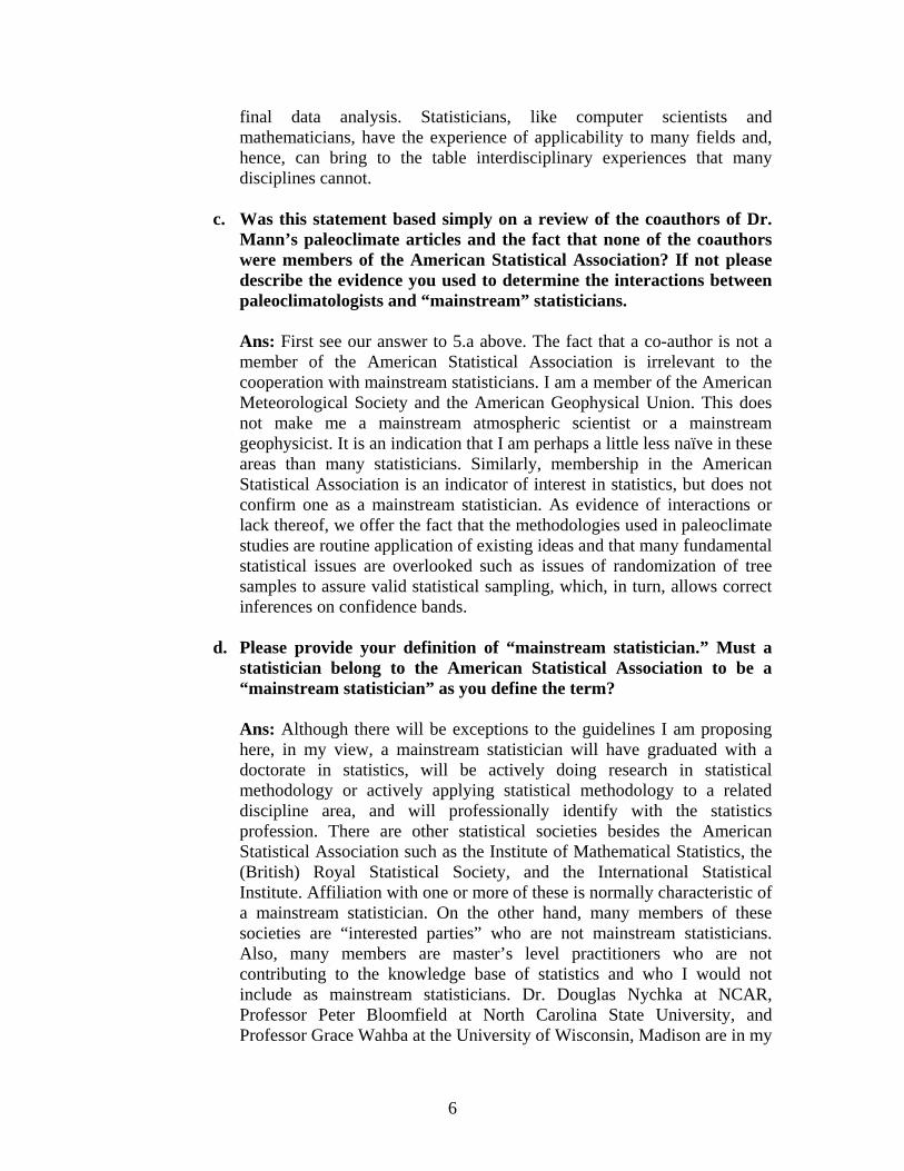
final data analysis. Statisticians, like computer scientists and mathematicians, have the experience of applicability to many fields and, hence, can bring to the table interdisciplinary experiences that many disciplines cannot.

c. Was this statement based simply on a review of the coauthors of Dr.

Mann’s paleoclimate articles and the fact that none of the coauthors were members of the American Statistical Association? If not please describe the evidence you used to determine the interactions between paleoclimatologists and “mainstream” statisticians.

Ans: First see our answer to 5.a above. The fact that a co-author is not a member of the American Statistical Association is irrelevant to the cooperation with mainstream statisticians. I am a member of the American Meteorological Society and the American Geophysical Union. This does not make me a mainstream atmospheric scientist or a mainstream geophysicist. It is an indication that I am perhaps a little less naïve in these areas than many statisticians. Similarly, membership in the American Statistical Association is an indicator of interest in statistics, but does not confirm one as a mainstream statistician. As evidence of interactions or lack thereof, we offer the fact that the methodologies used in paleoclimate studies are routine application of existing ideas and that many fundamental statistical issues are overlooked such as issues of randomization of tree samples to assure valid statistical sampling, which, in turn, allows correct inferences on confidence bands.

d. Please provide your definition of “mainstream statistician.” Must a

statistician belong to the American Statistical Association to be a “mainstream statistician” as you define the term?

Ans: Although there will be exceptions to the guidelines I am proposing here, in my view, a mainstream statistician will have graduated with a doctorate in statistics, will be actively doing research in statistical methodology or actively applying statistical methodology to a related discipline area, and will professionally identify with the statistics profession. There are other statistical societies besides the American Statistical Association such as the Institute of Mathematical Statistics, the (British) Royal Statistical Society, and the International Statistical Institute. Affiliation with one or more of these is normally characteristic of a mainstream statistician. On the other hand, many members of these societies are “interested parties” who are not mainstream statisticians. Also, many members are master’s level practitioners who are not contributing to the knowledge base of statistics and who I would not include as mainstream statisticians. Dr. Douglas Nychka at NCAR, Professor Peter Bloomfield at North Carolina State University, and Professor Grace Wahba at the University of Wisconsin, Madison are in my

7

view mainstream statisticians with a demonstrated interest and collaboration in the atmospheric sciences.

e. Please list all the authors in paleoclimate studies with whom you or

your coauthors spoke regarding the paleoclimatologists’ training in statistics and their consultations with statisticians (including statisticians who are not members of the American Statistical Association). For each author listed, please summarize the information he or she provided about statistics or statisticians and the paleoclimatology research committee.

Ans: I spoke with no one in paleoclimate studies. To the best of my knowledge neither have my colleagues. My home university, George Mason University, does have a Ph.D. program in climate dynamics. There are no requirements to take any statistics courses even though their principal interest is in climate modeling. According to the website of the Department of Meteorology at Pennsylvania State University (Michael Mann’s institution), there is no requirement to take a statistics course for the Ph.D. in meteorology (except possibly internal courses taught by meteorology faculty). The Department of Environmental Sciences at the University of Virginia (Dr. Mann’s previous institution) also does not explicitly specify any statistics courses. The graduate meteorology program at Iowa State University (with one of the strongest statistics departments in the nation) has no statistics requirements except a freshman-level statistics introductory course as a prerequisite to one of their graduate-level courses. The Department of Geology and Geophysics at Yale University where Dr. Mann obtained his Ph.D. also specifies no statistics courses. Indeed, they specify no courses at all except with the concurrence of an advisor5.

6. You testified that other scientists or statisticians reviewed your report before

it was sent to the Committee on Energy and Commerce, but it was unclear whether you provided a complete list. Please list the people who reviewed your report before it was sent to Committee, including name, title, area of expertise, and university or other affiliation.

• Professor (emeritus) Enders Robinson, geophysics, Columbia

University, elected member of the National Academy of Engineering

5 Indeed, we observe in the acknowledgement section of Dr. Mann’s dissertation that he credits Professor Jeffrey Park for Dr. Mann’s statistical training. Dr. Mann states, “… when my knowledge and skills in time series analysis and statistics were few. He taught me the tools of statistical data analysis.” Professor Park is a seismologist, not a statistician. Dr. Park received his doctorate in Earth Sciences from the University of California, San Diego.

8

• Professor Grace Wahba, statistics, University of Wisconsin, Madison, elected member of the National Academy of Science

• Professor Noel Cressie, spatial statistics, Ohio State University • Professor David Banks, statistics, Duke University, Editor of

Applications Section, Journal of the American Statistical Association

• Professor William Wieczorek, geophysics, Buffalo State SUNY • Dr. Amy Braverman, Senior Scientist, remote sensing, data

mining, Jet Propulsion Laboratory (CalTech) • Dr. Fritz Scheuren, statistics, NORC, University of Chicago, the

100th president of the American Statistical Association • In addition, we had two other reviewers who asked that their

names not be revealed because of potential negative consequences for them.

7. Prior to sending your report to the Committee on Energy and Commerce,

was your report peer reviewed, i.e. did someone other than the authors select the reviewers, were reviewers allowed to submit comments anonymously, was someone other the authors involved in deciding whether the authors’ responses were adequate?

Ans: Our report was not peer reviewed in the sense you ask. The review process we went through was similar to that employed by the National Research Council. At the NRC, the Committee makes recommendations to the Committee Chair and the Study Director. The list is narrowed and a recommendation is made by the Study Director. This list is approved by a higher-level authority and the document is sent out for review. The reviewers are not anonymous and their names are listed in the document. This was true of the recent North Study on Paleoclimate Reconstruction that was also the subject of our first round of testimony. Because we did not have the NRC structure, we obviously did not have a higher-level review of our list, but to the best of our ability, we acted in good faith to obtain reviews, some of which expressed dissenting opinions. Subsequently, we have been preparing papers that will be peer reviewed for the Applications Section of the Journal of the American Statistical Association, another for the journal called Statistical Science6 published by the Institute of Mathematical Statistics, and finally for a more popular outlet called Chance. In addition, we are preparing a paper motivated by our social network studies on the styles of co-authorship.

8. You testified that “the fact is that the peer review process failed in the 1998

paper.” Which peer review process were you referring to? Were you referring to the peer review process conducted by the journal that published the 1998 paper?

6 The Statistical Science article will have even more rigorous scrutiny than a normal peer review. It will be a discussion paper meaning that discussants will have an opportunity to comment in writing for the audience to see.

9

Ans: Yes, I was referring to the peer review process at Nature, which published the 1998 paper.

9. Your analysis seems to show that, at least in some instances, when you use

the same methodology and the same data, a graph of the results will look like a hockey stick when the data is decentered, but not when the data is properly centered.

a. Is that a correct statement?

Ans: Yes. We explicitly looked at the first principal component of the North American Tree Ring series and demonstrated that the hockey stick shows up when the data are decentered, but not when properly centered. We also demonstrated the same effect with the digitized version of the 1990 IPCC curve.

b. Does your analysis prove that every time you use improperly centered

data and the climate field reconstruction methodology (CFR) and get a hockey stick, the hockey stick will disappear when the data is properly centered? Or does the shape of the graph with properly centered data depend on the data?

Ans: The shape of the graph will depend on the underlying data. To reiterate our testimony, the decentering process as used in MBH98 and MBH99 selectively prefers to emphasize the hockey stick shape. This is because the decentering increases the apparent variance of hockey sticks and principal component methods attempt to find components with the largest explainable variance. If the variance is artificially increased by decentering, then the principal component methods will “data mine” for those shapes. In other words, the hockey stick shape must be in the data to start with or the CFR methodology would not pick it up. What we have shown both analytically and graphically in Figure 4.6 is that using the CFR methodology, just one signal when decentered will overwhelm 69 independent noise series. The point is that if all 70 proxies contained the same temperature signal, then it wouldn’t matter which method one used. But this is very far from the case. Most proxies do not contain the hockey- stick signal. The MBH98 methodology puts undue emphasis on those proxies that do exhibit the hockey-stick shape and this is the fundamental flaw. Indeed, it is not clear that the hockey-stick shape is even a temperature signal because all the confounding variables have not been removed.

c. Does your report prove that “the hockey stick disappears” from

MBH98 and MBH99 if one were to fix the decentering? In other words, does your paper prove that “the hockey stick disappears” if the data is properly centered but the rest of the MBH98 and MBH99

10

analysis were kept the same (i.e., it relied on the CFR methodology and all the proxy data used by Dr. Mann in MBH98 and MBH99)? If you believe that it does, what level of certainty do you give to this conclusion?

Ans: Our report does not prove that the hockey stick disappears. Our work demonstrates that the methodology is incorrect. Because of the lack of proper statistical sampling and correct inferential methodology, we concluded that the statements regarding the decade of the 1990s probably being the hottest in a millennium and 1998 probably being the hottest year in a millennium are unwarranted. Indeed, I repeatedly testified that the instrumented temperature record from 1850 onwards indicated that there is a pattern of global warming. We have never disputed this. We also believe that there is no dispute between our report and the North report in this regard. Professor North in testimony agreed with our conclusions regarding the incorrectness of the methodology. We in turn agree with the fundamental conclusion of the North report, i.e. that the present era is likely the hottest in the last 400 years. We remain silent on the issues related to anthropogenic global warming.

d. Does your report include a recalculation of the MBH98 and MBH99

results using the CFR methodology and all the proxies used in MBH98 and MBH99, but properly centering the data? If not, why doesn’t it?

Ans: Our report does not include the recalculation of MBH98 and MBH99. We were not asked nor were we funded to do this. We did not need to do a recalculation to observe that the basic CFR methodology was flawed. We demonstrated this mathematically in Appendix A of the Wegman et al. Report. The duplication of several years of funded research of several paleoclimate scientists by several statisticians doing pro bono work for Congress is not a reasonable task to ask of us. We all have additional responsibilities to the people and agencies that pay our salaries.

10. In the footnote of your report, you reference papers by Wahl and Ammann

(2006) and Wahl et al. (2006) and note that they “are not to the point.” I understand that Wahl and Ammann actually examined, among other things, the problem of data decentering, the main focus of your report, and corrected the emulation of MBH98 by recentering the data.

a. Did you analyze this work by Wahl and Ammann prior to sending

your final report to the Committee on Energy and Commerce? If so, why does your report not alert the reader that these researchers had conducted a reanalysis of the MBH98 that corrected the only statistical methodology error discussed in the “Finding” section of

11

your report and that these researchers found that recentering the data did not significantly affect the results reported in the MBH98 paper?

Ans: The Wahl and Ammann paper came to our attention relatively late in our deliberations, but was considered by us. Some immediate thoughts we had on Wahl and Ammann was that Dr. Mann lists himself as a Ph.D. co-advisor to Dr. Ammann on his resume. As I testified in the second hearing, the work of Dr. Ammann can hardly be thought to be an unbiased independent report. It would have been more convincing had this paper been written by a totally independent authority, but alas this is not the case. The Wahl and Ammann paper is largely an attempt to refute the criticisms of McIntyre and McKitrick (MM). The comment we made in our footnote about being ‘not to the point” refers to the fact that MM03 and MM05 were not attempting to portray themselves as doing a paleoclimate reconstruction, they not being paleoclimatologists themselves, but were merely pointing out the flaws in the MBH98 and MBH99 papers. There are several comments of interest in the Wahl and Ammann paper. They suggest three areas in which the MBH papers have been subject to scrutiny. “First, the MBH reconstruction has been examined in light of its agreement/lack of agreement with other long-term annual and combined high/low frequency reconstructions.” Wahl and Ammann (2006, p.3 in the 24 February 2006 draft) Their conclusion is: “The comparison of the MBH reconstruction, derived from multi-proxy (particularly tree ring) data sources, with widespread bore-hole-based reconstructions … is still at issue in the literature.” Wahl and Ammann (2006, p.4 in the 24 February 2006 draft) In other words, the MBH reconstruction does not agree with other widely accepted methodologies for climate reconstruction. Bore hole methods measure a temperature gradient and calculate the diffusion of heat within the bore hole. This method does not have nearly the confounding variables as do tree ring proxies. The second area of scrutiny involves comparison with results from modeling efforts. “Second a related area of scrutiny of the MBH reconstruction technique arises from an atmosphere-ocean general circulation model (AOGCM) study …, which also examines the potential loss of amplitude [in the MWP] in the MBH method (and other proxy/instrumental reconstructions that calibrate by using least squares projections of the proxy vectors onto a single- or multi-dimensional surface determined by either the instrumental data or its [their] eigenvectors.” Wahl and Ammann (2006, p.4 in the 24 February 2006 draft) Again the MBH reconstructions do not correlate well with the model-based methods. Wahl and Amman (2006) offer the following explanation.

12

“However, a number of issues specific to the modeling situation could arise in this context, including: how realistically the AOGCM is able to reproduce the real world patterns of variability and how they respond to various forcings7; the magnitude of forcings and the sensitivity of the model that determine the magnitude of temperature fluctuations …; and the extent to which the model was sampled with the same richness of information that is contained in the proxy records (not only temperature records, but series that correlate well with the primary patterns of variability – including, for example, precipitation in particular seasons.” Wahl and Ammann, (2006, p.5 in the 24 February 2006 draft) This quotation has two interesting facets. First, it seems to call into question the very models that are predicting temperature increases based on CO2 forcings. If these models do not coincide with the MBH reconstructions, then which are we to believe? Second, the quotation implicitly admits what we have observed previously, namely that there are other covariates such as precipitation, which are not teased out in the temperature reconstructions. Thus, what are purported to be temperature reconstructions are contaminated with covariates that reflect temperature indirectly at best and not at all at worst. The third area of scrutiny involves the challenges made by MM. “A third area of scrutiny has focused on the nature of the proxy data set utilized by MBH, along with the pre-processing algorithms used to enhance the climate signal-to-noise characteristics of the proxy data.” Wahl and Ammann, (2006, p.5 in the 24 February 2006 draft) We submit that both the mathematical analysis in Appendix A of our report to Congress together with our simulation demonstrate that the decentering method yields incorrect results. The critical issue then becomes the proxies themselves, which MM have challenged. A telling comment from Wahl and Ammann is the following. “A further aspect of this critique is that the single-bladed hockey stick shape in proxy PC summaries for North America is carried disproportionately by a relative small subset (15) of proxy records derived from bristlecone/foxtail pines in the western United States, which the authors [MM] mention as being subject to question in the literature as local/regional temperature proxies after approximately 1850 …. It is important to note in this context that because they employ an eigenvector-based CFR technique, MBH do not claim that all proxies used in their reconstruction are closely related to local-site variations in surface temperature.” Wahl and Ammann, (2006, p.9 in the 24 February 2006 draft). This together with the AOGCM quotation reinforces the notion that MBH are attempting to reconstruct temperature histories based on proxy data that are extremely problematic in terms of actually capturing temperature information directly. As we testified, it would seem that there is some substantial likelihood that the bristlecone/foxtail pines are CO2 fertilized and hence are reflecting not temperature at all but CO2 concentration. It is a circular argument to say increased CO2 concentrations are causing

7 Including presumably forcings from greenhouse gasses such as CO2.

13

temperature increases when temperature increases are estimated by using proxies that are directly affected by increased CO2 concentrations. It is our understanding that when using the same proxies as and the same methodology as MM, Wahl and Ammann essentially reproduce the MM curves. Thus, far from disproving the MM work, they reinforce the MM work. The debate then is over the proxies and the exact algorithms as it always has been. The fact that Wahl and Ammann (2006) admit that the results of the MBH methodology does not coincide with the results of other methods such as borehole methods and atmospheric-ocean general circulation models and that Wahl and Ammann adjust the MBH methodology to include the PC4 bristlecone/foxtail pine effects are significant reasons we believe that the Wahl and Amman paper does not convincingly demonstrate the validity of the MBH methodology.

b. Do you agree or disagree with Wahl and Ammann’s finding that the time period used to center the data does not significantly affect the results reported in the MBH98 paper? If you disagree, please state the basis for your disagreement.

Ans: We do disagree. The fundamental issue focuses on the North American Tree Ring proxy series, which Wahl and Ammann admit are problematic in carrying temperature data. In the original MBH decentered series, the hockey-stick shape emerged in the PC1 series because of reasons we have articulated in both our report and our testimony. In the original MBH papers, it was argued that this PC1 proxy was sufficient. We note the following from Wahl and Ammann. “Thus, the number of PCs required to summarize the underlying proxy data changes depending on the approach chosen. Here we verify the impact of the choice of different numbers of PCs that are included in the climate reconstruction procedure. Systematic examination of the Gaspé-restricted reconstructions using 2-5 proxy PCs derived from MM-centered, but unstandardized data demonstrates changes in reconstruction as more PCs are added, indicating a significant change in information provided by the PC series. When two or three PCs are used, the resulting reconstructions (represented by scenario 5d, the pink (1400-1449) and green (1450-1499) curve in Fig. 3) are highly similar (supplemental information). As reported below, these reconstructions are functionally equivalent to reconstructions in which the bristlecone/foxtail pine records are directly excluded [emphasis added] (cf. pink/blue curve for scenarios 6a/b in Fig. 4). When four or five PCs are used, the resulting reconstructions (represented by scenario 5c, within the thick blue range in Fig. 3) are virtually indistinguishable (supplemental information) and are very similar to scenario 5b.” Wahl and Ammann, (2006, p.31, 24 February 2006 draft) Without attempting to describe the technical detail, the bottom line is that, in the MBH original, the hockey stick emerged in PC1 from the bristlecone/foxtail pines. If one centers the data properly the hockey stick

14

does not emerge until PC4. Thus, a substantial change in strategy is required in the MBH reconstruction in order to achieve the hockey stick, a strategy which was specifically eschewed in MBH. In Wahl and Ammann’s own words, the centering does significantly affect the results.

c. Dr. Gulledge included in his testimony a slide showing the graph of W

A emulation of the MBH and MBH-corrected for decentering and the Gaspe tree-ring series. Were you aware of their reanalysis of MBH99 prior to the time you finalized your report? Do you agree or disagree with their reanalysis of MBH99? If you disagree, please state the basis for your disagreement.

Ans: Yes, we were aware of the Wahl and Ammann simulation. We continue to disagree with the reanalysis for several reasons. Even granting the unbiasedness of the Wahl and Ammann study in favor of his advisor’s methodology and the fact that it is not a published refereed paper, the reconstructions mentioned by Dr. Gulledge, and illustrated in his testimony, fail to account for the effects of the bristlecone/foxtail pines. Wahl and Ammann reject this criticism of MM based on the fact that if one adds enough principal components back into the proxy, one obtains the hockey stick shape again. This is precisely the point of contention. It is a point we made in our testimony and that Wahl and Ammann make as well. A cardinal rule of statistical inference is that the method of analysis must be decided before looking at the data. The rules and strategy of analysis cannot be changed in order to obtain the desired result. Such a strategy carries no statistical integrity and cannot be used as a basis for drawing sound inferential conclusions.

11. Please answer the following questions with respect to Figure 4.3 in your

report:

a. Is the data centering the only difference between the two panels in that figure?

Ans: Yes, the centering is the only difference.

b. Were the same R commands used to carry out the PC analysis for the

upper and lower panels?

Ans: Yes, the same R commands were used except that a parameter indicating centering or not was adjusted.

c. Was the upper frame processed based on a correlation matrix? Was

the lower frame processed based on a covariance matrix? If the answer to both questions is yes, does this not have the effect of comparing standardized with non-standardized data?

15

Ans: The correct method for a principal component analysis (that we executed) is to use the covariance matrix and not the correlation matrix. The correlation is a scaled version of the covariance divided by the product of the standard deviations of the individual variables. You are really asking a different processing question when you ask about standardized versus non-standardized data. Because the scale of different proxy series is different, as indicated above PCA will preferentially emphasize series with larger variance as the first principal component. Thus, it is important to ensure that the proxy data all have the same scale. This is a tricky adjustment from a statistical perspective. Simply dividing by the standard deviation is a non-robust procedure if the data have outliers. This appears to be the case with many of the proxy data sets. Thus, a robust estimator of scale must be used. One can observe that we did do the scale adjustment based on the fact that the scales of the Y axes are approximately the same. The underlying assumption is that the time series of proxy data are heteroscedastic, which is a fancy statistical term meaning that they have the same variance (scale) through time. This is also a problematic assumption for serious data analyses, although it is the approximation made by MBH and by us to generate Figure 4.3.

d. Is it appropriate to compare data sets that have more than a tenfold

difference in standard deviation among them? Would not such a comparison preferentially select data sets with larger variance, regardless of the climate signal contained in the data sets with the smaller variance?

Ans: No, it is not appropriate and we did not do this. Yes indeed, the PCA would over-represent proxies with a larger variance to the detriment of climate signals in sets with smaller variance. Again, we did not do this.

e. What does PC1 look like if the data are centered correctly and

processed based on a correlation matrix instead of a covariance matrix?

Ans: If the scale is adjusted by the standard deviation after first being centered, then the result is a standardized random vector. In this case, the covariance matrix would be identical with the correlation matrix and would look like the bottom panel of our Figure 4.3.

16

APPENDIX A: Wegman Social Network Analysis

Edward J. Wegman’s Author−Coauthor Social Network

Walid Sharabati

Introduction

Social Networks are becoming an important tool in analyzing the behavior of groups of peo-ple on the global level (how one or more group interacts with other group(s)) and on the locallevel (how individuals interact with each other within the same network.) In this report,we will study in depth the author-coauthorship social network of Edward J. Wegman – aprominent professor of Statistics at George Mason University, Fairfax VA, USA.

We would like to provide you some background on Dr. Wegman. He received his Ph.D.degree in Mathematical Statistics from University of Iowa in 1968. Immediately after hisPh.D., he went to the statistics department at the University of North Carolina, ChapelHill, which was one of the leading statistics departments in the world. His early career fo-cused on the development of aspects of the theory of mathematical statistics. In 1978, hewent to the Office of Naval Research (ONR) where he was the Head of the MathematicalSciences Division. He has been in the research and academia field for some time and haspublished an array of work, which includes over 200 prestigious refereed journals, books, andtechnical reports, authored individually and with a number of colleagues and Ph.D. students.

In this study, we are going to look at the structure of the network and model its behav-ior. The objective of this paper is to perform a comprehensive social network analysis onthe first-level of Wegman’s coauthorship network.

Social Networks can be treated as directed graphs in which actors (individuals) are repre-sented by vertices (nodes) while interactions between actors are represented by edges (ties),which may have weights. There are three basic representations of a graph – the planargraph visualization, the adjacency matrix, and the sparse-graph representation. The toolsand methods of analyzing graphs will be covered in detail in Section 3.

1 Literature Review

It is worth mentioning that no one has yet analyzed Wegman’s author-coauthorship socialnetwork on any level. This work will provide an independent source to view the network onthe different levels and examine how the actors interact with each other. It is the expectationthat the methodology and techniques applied will unveil important properties of the network.

1

Figure 1: Snapshot of the proximity adjacency matrix.

Figure 2: Snapshot of the proximity adjacency matrix of the coauthors with frequency ≥ 5.

Of all the work that has been done on social networks, very few investigators have con-sidered coauthorship network. Therefore, what we are about to observe in this paper is abrand new approach in the social networks field.

The main purpose of analyzing coauthorship networks is to be able to answer the ques-tion of “who-wrote-with-who” with what frequency.

2 Data

Wegman’s raw data was collected directly from his personal website and his updated cur-riculum vitae. Building the adjacency/proximity matrix manually was very cumbersomebecause one has to consider not only Wegman and his coauthors and the coauthors whowrote with other coauthors, but also the frequency of communication. It is vital to keeptrack of the record of every coauthor.

Figure 1 is a snapshot of one block of the proximity adjacency matrix built in MS-Excel, theoriginal matrix is of size 102× 102. Notice that the matrix is symmetric due to the fact thatrelationship among actors are reflexive; i.e. if person A published with person B then thisalso implies person B published with person A.

Figure 2 shows a list of all coauthors published with Wegman five times or more.

2

Figure 3: Wegman’s author-coauthor social network.

3 Analysis Methods

The methodology adopted in this study consists of both theoretical approach to quantita-tively analyze the network, and software approach to simulate and visualize the network.The algorithms and techniques applied to study interactions within the network includecentrality measures (node degree and closeness), network partitioning (cliques and cliqueoverlapping), network connectivity (cut-points and bridges), structural equivalence, struc-tural holes, brokerage roles and block-modeling. The software tools used to run and modelthe network are UCINET-6 and Pajek-1.02.

4 Results and Discussion

We start by exploring Wegman’s network with all the actors (coauthors) followed by a de-tailed analysis pinning down the significant and interesting characteristics of the network.The general structure of the network is based on a weighted digraph consisting of nodes(coauthors) and weighted edges (ties) representing the number of times an actor coauthored

3

Figure 4: Example of a simple ego-network. Node Ego has degree = 7, nodes A and C have both degree =2, nodes B, D, E, F and G have all degree = 1.

with Wegman and with other coauthors. Figure 3 shows the basic structure of Wegman’snetwork. The graph suggests that the network is an “ego” network; in which all nodes areconnected to one focal node, see Figure 4. In graph theory terms this referred to as a stargraph. This star shape is predicted in first-level coauthorship networks since all coauthorsare expected to have communicated (ties) with that one main author. The current number ofactors coauthored with Wegman is 101. Some coauthors share edges not only with Wegman,but also with other coauthors; more than one name can appear on a publication. One canclearly see the two “clouds” (clump networks) fully connected – complete subgraphs.

Figure 5 shows the matrix representation of Wegman’s network, each black square indicatesa coauthor-relation. The matrix is generated using Pajek.

Figure 6 shows the network in circle layout, the coloring and thickness of both the nodes andedges will be discussed more when we analyze centrality measures and network partitioning.Circle layout is yet another way of displaying the network.

Figure 7 is a random partition of the network with two clusters in grey scale, the darker thecolor the higher the frequency. Figure 8 is a random partition of the network with threeclusters.

4.1 Centrality Measures

In social networks analysis, centrality measures are quantitative tools used for investigatingthe network; the two centrality metrics that we are applying are node degree and closeness.At the individual level, one dimension of position in the network can be captured throughcentrality. Conceptually, centrality is straight forward; we want to identify the nodes resid-ing in the “center” of the network.

4

Figure 5: Adjacency matrix of Wegman’s network.

5

Figure 6: Circle layout of Wegman’s network.

Degree of a node is the number of edges that connect it to other nodes; see Figure 4, degreecan be interpreted as measure of power or importance of a node, or measure of workload.The actor with most ties is the most important figure in a network. In a simple randomgraph, degree will have a Poisson distribution [2], and the nodes with high degree are likelyto be at the intuitive center. Deviations from a Poisson distribution suggest non-randomprocesses, which is at the heart of current “scale-free” work on networks.

Definition: A graph G, is a collection of nodes N and edges E; G = {N, E}, whereN = {n1, n2, n3, · · · , nk} and E = {e1, e2, e3, · · · , eE}.

Definition: Node degree; denoted Cd(ni), is defined by

Cd(ni) = d(ni) =∑

j

aij, aij ∈ A, (1)

where d represents degree measure, and A is the adjacency matrix.

To illustrate the degree measure, we calculate the node degree for the nodes in Figure 4.The table below shows the results.

6

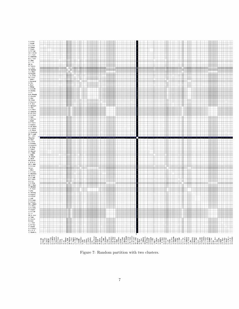
Figure 7: Random partition with two clusters.

7

Figure 8: Random partition with three clusters.

8

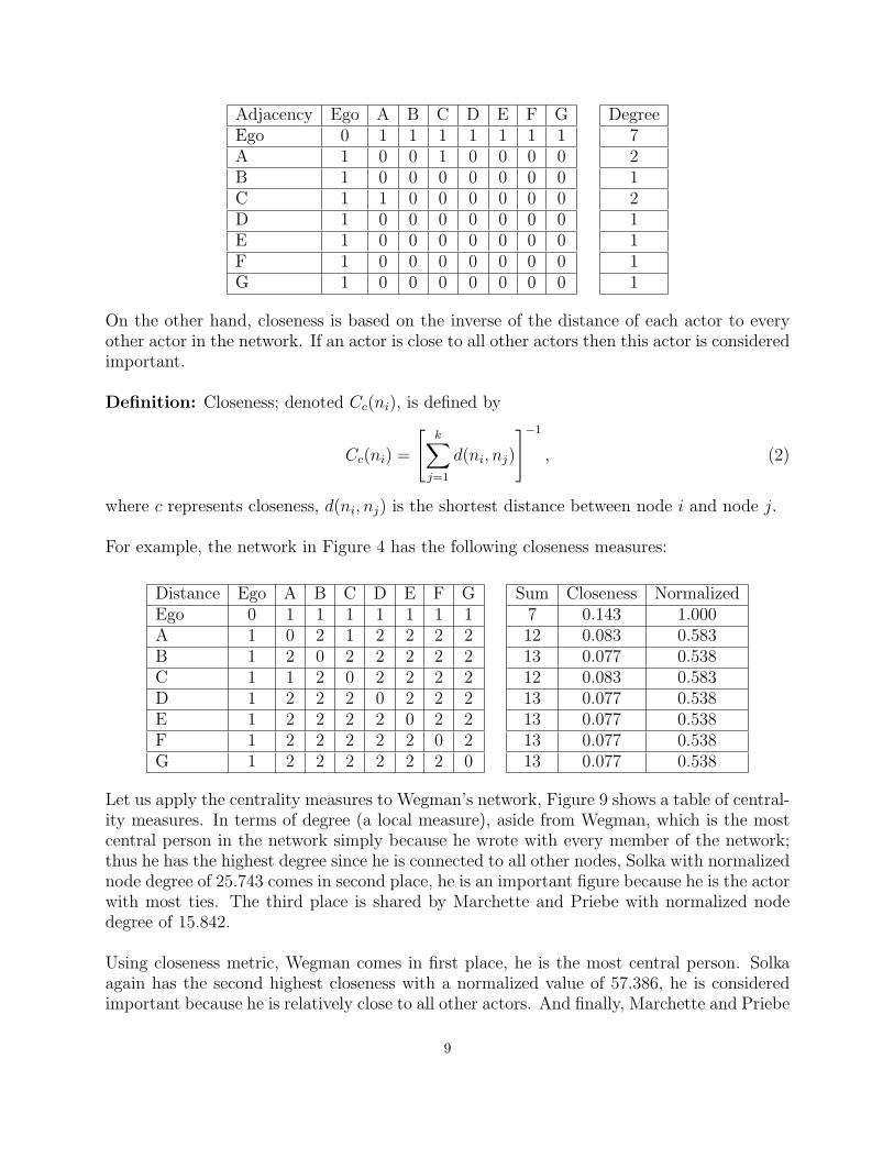
Adjacency Ego A B C D E F GEgo 0 1 1 1 1 1 1 1A 1 0 0 1 0 0 0 0B 1 0 0 0 0 0 0 0C 1 1 0 0 0 0 0 0D 1 0 0 0 0 0 0 0E 1 0 0 0 0 0 0 0F 1 0 0 0 0 0 0 0G 1 0 0 0 0 0 0 0

Degree72121111

On the other hand, closeness is based on the inverse of the distance of each actor to everyother actor in the network. If an actor is close to all other actors then this actor is consideredimportant.

Definition: Closeness; denoted Cc(ni), is defined by

Cc(ni) =

[k∑

j=1

d(ni, nj)

]−1

, (2)

where c represents closeness, d(ni, nj) is the shortest distance between node i and node j.

For example, the network in Figure 4 has the following closeness measures:

Distance Ego A B C D E F GEgo 0 1 1 1 1 1 1 1A 1 0 2 1 2 2 2 2B 1 2 0 2 2 2 2 2C 1 1 2 0 2 2 2 2D 1 2 2 2 0 2 2 2E 1 2 2 2 2 0 2 2F 1 2 2 2 2 2 0 2G 1 2 2 2 2 2 2 0

Sum Closeness Normalized7 0.143 1.00012 0.083 0.58313 0.077 0.53812 0.083 0.58313 0.077 0.53813 0.077 0.53813 0.077 0.53813 0.077 0.538

Let us apply the centrality measures to Wegman’s network, Figure 9 shows a table of central-ity measures. In terms of degree (a local measure), aside from Wegman, which is the mostcentral person in the network simply because he wrote with every member of the network;thus he has the highest degree since he is connected to all other nodes, Solka with normalizednode degree of 25.743 comes in second place, he is an important figure because he is the actorwith most ties. The third place is shared by Marchette and Priebe with normalized nodedegree of 15.842.

Using closeness metric, Wegman comes in first place, he is the most central person. Solkaagain has the second highest closeness with a normalized value of 57.386, he is consideredimportant because he is relatively close to all other actors. And finally, Marchette and Priebe

9

Figure 9: Normalized nodes degree and closeness for all actors.

10

have a closeness normalized value of 54.301, which puts them in third place. W. Martinezwith a normalized closeness value of 53.723 comes in fourth place. Notice that no othercoauthor has a normalized closeness value less than 50.249. There are two reasons for that,one is that we are considering only first level coauthorship, which means that most actorswill relatively have similar values and close to that one author, and secondly, one shouldkeep in mind that the Wegman’s network is a star graph with one main figure in the center.We expect the second level coauthorship network to act differently and provide more insighton the dynamics of this network.

Figure 10 is a modified version of Figure 3 emphasizing nodes degree and tie strength.Nodes color and size are set by the attribute node degree, while edges color and thicknessare set by the attribute tie strength, which represents frequency of communication. Colorpalettes of nodes degree and ties strength are shown in Figure 11. As we mentioned earlierSolka has the second largest node degree, note that Priebe and Marchette have the samenode color and size since they are in third place. Also, we can see that W. Martinez andLuo have relatively large nodes with the same node color. Yet, if we consider ties strengthinstead; clearly Solka has the highest frequency then comes W. Martinez in second place. Inparallel, another interesting hidden feature is revealed by the graph, Solka and W. Martinezhave the strongest tie among all coauthors, they wrote with each other (17 times) more thanany other two coauthors did in the network excluding Wegman. The edges (Solka, Priebe)and (Solka, Marchette) have the same color and thickness, which suggests that Priebe andMarchette coauthored with Solka the same number of times, in fact, they coauthored fourtimes. Note that any two or more nodes or edges have the same color and/or thickness implythat they have the same node degree and/or tie strength.

Definition: Graph diameter is the longest geodesic between any two nodes, where the geo-desic is the length of the shortest path between any two nodes.

The diameter of Wegman’s network is 2, this is simply because the network is a star graphand because we are just studying the first-level network.

Definition: Graph density is defined as the ratio of number of edges in the graph to thetotal possible number of edges in a graph.

D =E

k(k − 1)/2=

2E

k(k − 1)(3)

Using UCINET-6, Wegman’s network graph density is 0.0986.

4.2 Network Connectivity

Definition: A dyad is a pair of nodes and the edge connecting them.

Definition: A triad is a set of three nodes and the edges connecting them.

A triad is identified by a M-A-N number system of three digits and a letter. The first

11

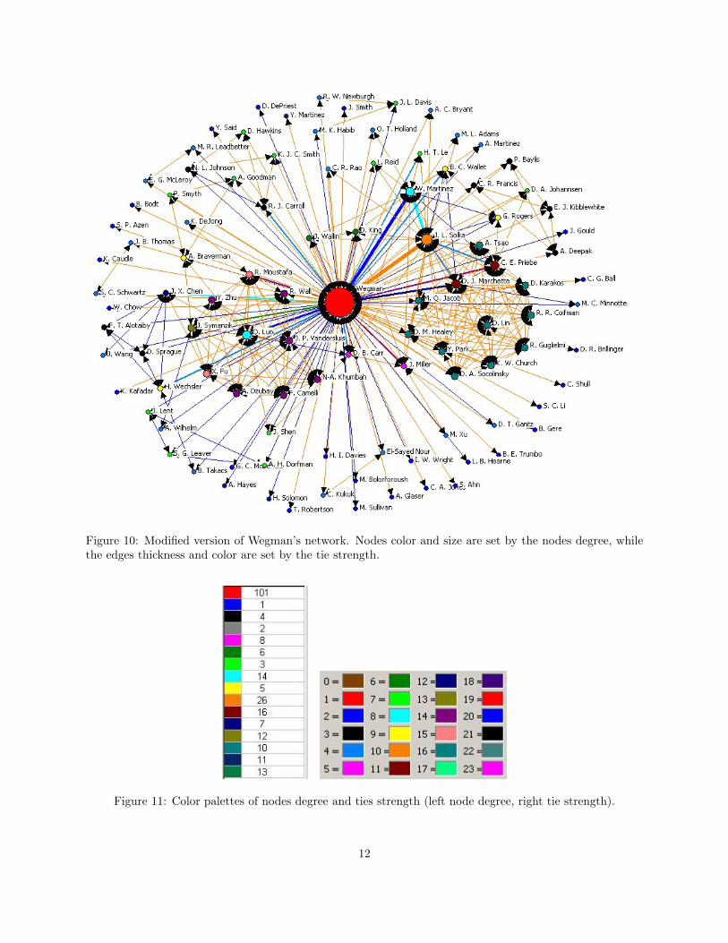
Figure 10: Modified version of Wegman’s network. Nodes color and size are set by the nodes degree, whilethe edges thickness and color are set by the tie strength.

Figure 11: Color palettes of nodes degree and ties strength (left node degree, right tie strength).

12

Figure 12: Wegman’s network without Wegman.

digit indicates the number of mutual positive dyads (M), the second digit is the number ofasymmetric dyads (A), and the third digit is the number of null dyads (N). Sometimes, aletter which refers to the direction of the asymmetric choices is added to distinguish betweentriads with the same M-A-N labeling digits: D for down, U for up, C for cyclic, and T fortransitive [3].

We then examine the network without the star node Wegman in attempt to discover sec-ondary structure and how the network behaves without the main actor. Figure 12 showsthis network without Wegman. The graph is now partially disconnected with a number ofisolated nodes; in this case, Wegman is considered a cutpoint and the edges {(Carr, Luo),(Carr, Shen)} are considered local bridges. Notice that it is less frequent to find globalbridges. Both of Carr and Luo are cutpoints; by removing either of these nodes the sub-network will be disconnected. Triads are obvious in this network; for instance, the triad300 (mutual actors agreeing) {(Carr, Shen, Luo)}, which also forms a clique, is vital to thenetwork in the sense that by removing this clique the network will be further disconnectedand thus have more than one component (maximal connected subgraph). We will discusscliques more in section 4.3.

Some actors are still connected with others forming subnetworks. The actors {(Lent, Leaver,Dorfman)} form again the triad 300; also known as triad 16, it refers to the structure withreciprocal links (A writes with B and B writes with A) among three different coauthors.

13

Figure 13: Wegman’s network with Wegman.

Figure 13 shows the network with Wegman.

4.3 Cohesive Subgroups

One of the most interesting features in a network that caught structural analysts’ attentionis secondary sub-structures such as network cohesion. Researchers interested in cohesive sub-groups gathered and studied sociometric data on affective ties in order to identify “cliquish”subgroups (face-to-face group). The clique is the foundational idea for studying and analyz-ing cohesive subgroups in social networks.

Definition: A clique in a graph is a maximal complete subgraph of three or more nodes,mutual dyads (2 nodes) are not considered to be cliques [4].

It consists of a subset of nodes all of which are adjacent to each other, and there are noother nodes that are also adjacent to all of the members of the clique. A clique is a verystrict definition of cohesive subgroups. Cliques are a subset of the network in which theactors are more closely and intensely tied to one another than they are to other members ofthe network and if one actor disappears for any reason, the other two can still write/talk toeach other. As an illustration, in Figure 4, the nodes {Ego, A, C} form a clique.

14

Figure 14: The 36 clique sets in Wegman’s network.

In Wegman’s network there are 36 cliques, Figure 14 shows all 36 clique sets with thecoauthors. For example, in the relations of coauthors, clique number 11 consists of thenodes (Wegman, Solka, Bryant), clique number 9 consists of the coauthors (Wegman, Solka,W. Martinez, Reid), clique number 2 consists of the actors (Wegman, Solka, W. Martinez,Marchette, Priebe). We can also observe that an actor can be a member of one or moreclique such as Solka.

Notice that cliques in a graph may overlap. The same node or set of nodes might belongto more than one clique (some cliques contain more than one member in common). Also,there may be nodes that do not belong to any cliques. However, no clique can be entirelycontained within another clique, because if it were the smaller clique then it would not bemaximal. Figure 15 shows the clique overlap. There is a considerable overlap among thecliques in the coauthor relation, more than one coauthor belongs to one or more cliques.

Cliques are interesting to study because suppose the actors in one network form two non-overlapping cliques; and that the actors in another network also form two cliques, but thatthe memberships overlap (some people are members of both cliques). Where the groupsoverlap, we might expect that conflict between them is less likely than when the groups donot overlap [1], this is the case with Wegman, Solka, W. Martinez and Marchette. Wherethe groups overlap, mobilization and diffusion may spread rapidly across the entire network;where the groups do not overlap, traits may occur in one group and not diffuse to the other.

15

Figure 15: The clique overlap in Wegman’s network.

4.4 Structural Equivalence

Definition: Two actors are structurally equivalent if they have the same type of ties to thesame people.

We now discuss the method of partitioning actors into subsets so that actors within eachsubset are closer to being equivalent than are actors in different subsets. One way to displaythe results of a series of partitions is to construct a dendrogram indicating the degree ofstructural equivalence among the positions and identifying their members. Each level of thediagram indicates the division resulting from a split of the previous subset [4]. A dendrogramthus represents a clustering of the actors, those actors who are connected by branches low inthe diagram are closer to being perfectly structurally equivalent, whereas subsets of actorswho are joined only through paths high up the diagram are less structurally equivalent (orare not equivalent at all). In brief, the lowest position in the diagram indicates that everyactor is different while the highest position indicates that all actors are the same; what is inbetween is more important in terms of structural equivalence. Figure 16 shows the clusterdiagram of Wegman’s network.

16

Figure 16: Dendrogram of Wegman’s network.

17

4.5 Blockmodeling

Definition: A blockmodel is the process of identifying positions in the network. A block isa section of the adjacency matrix “a group of people” structurally equivalent. It consists oftwo things according to Wasserman and Faust [4]:

• A partition of actors in the network into discrete subsets called positions.

• For each pair of positions a statement of the presence or absence of a tie within orbetween the positions on each of the relations.

A blockmodel is thus a hypothesis about a multirelational network. It presents generalfeatures of the network, such as the ties between positions, rather than information aboutindividual actors.

A blockmodel is a simplified representation of multirelational network that captures someof the general features of a network’s structure. Specifically, positions in a blockmodel con-tain actors who are approximately structurally equivalent. Actors in the same position haveidentical or similar ties to and from all actors in other positions. Thus, the blockmodel isstated at the level of the positions, not individual actors.

Figure 17 shows these two clumps clustered in the upper left corner of the adjacency matrix,there is a total of four clusters in the graph. Each member of these clusters in structurallyequivalent. The graph is based on random start blockmodeling applied on the network usingstructural equivalence while setting the number of cluster to be four.

5 Advanced Analysis

5.1 Discarding Weak Ties

We next present some discussion on the network excluding the edges having weight=1, i.e.all the coauthors who wrote with Wegman only once. The basic concept is that actorswho communicated “wrote” with Wegman only one time are most likely to be students whograduated and are no longer connected to Wegman in some sense or coauthors who haveweak ties with Wegman at the current time. In conclusion, these are the ones with minimalimpact on the network. We will assume that all the coauthors with tie strength being onehave not coauthored with Wegman and therefore will be treated as isolated nodes in thenetwork. Figure 18 shows the network without the edges with frequency = 1 together withthe corresponding edge weight. As before, nodes’ color and size are set by the attribute“node degree” while edges’ color and thickness are set by the attribute “tie strength”.

Figure 19 shows the cliques not including the nodes with edge weight=1, the number ofcliques is 14.

Figure 20 shows the network without Wegman. Clearly, the network is disconnected withfewer components. There are three subgroups that are still relatively strong, these subgroups

18

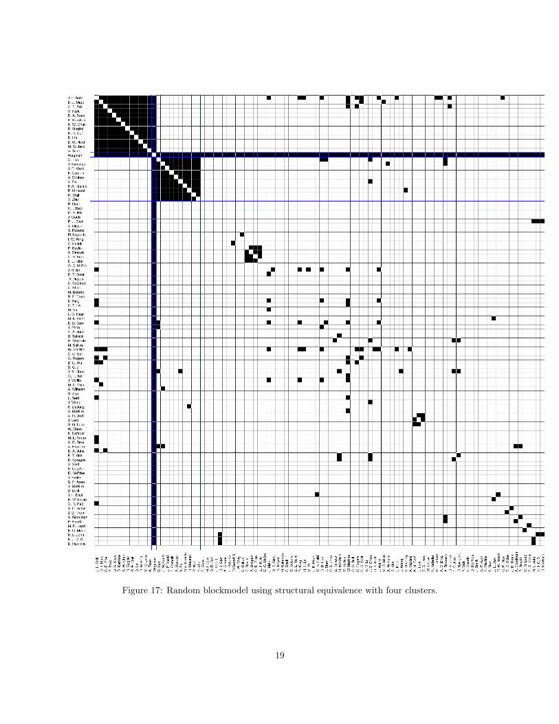
Figure 17: Random blockmodel using structural equivalence with four clusters.

19

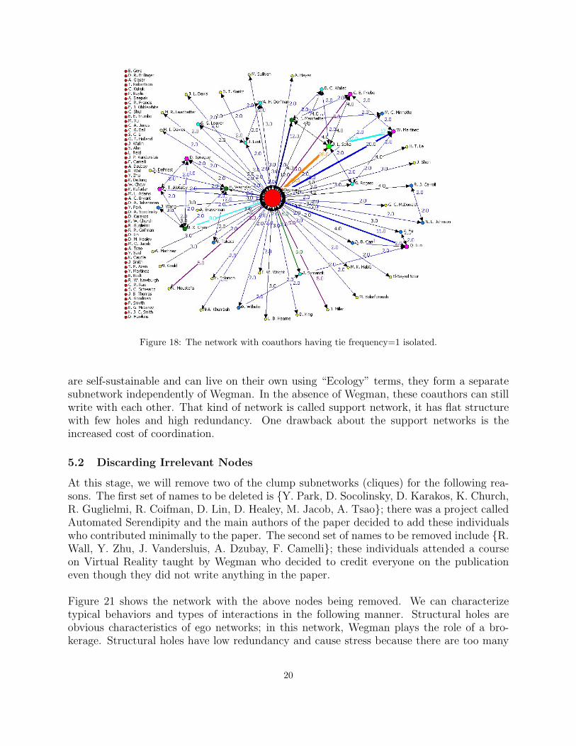
Figure 18: The network with coauthors having tie frequency=1 isolated.

are self-sustainable and can live on their own using “Ecology” terms, they form a separatesubnetwork independently of Wegman. In the absence of Wegman, these coauthors can stillwrite with each other. That kind of network is called support network, it has flat structurewith few holes and high redundancy. One drawback about the support networks is theincreased cost of coordination.

5.2 Discarding Irrelevant Nodes

At this stage, we will remove two of the clump subnetworks (cliques) for the following rea-sons. The first set of names to be deleted is {Y. Park, D. Socolinsky, D. Karakos, K. Church,R. Guglielmi, R. Coifman, D. Lin, D. Healey, M. Jacob, A. Tsao}; there was a project calledAutomated Serendipity and the main authors of the paper decided to add these individualswho contributed minimally to the paper. The second set of names to be removed include {R.Wall, Y. Zhu, J. Vandersluis, A. Dzubay, F. Camelli}; these individuals attended a courseon Virtual Reality taught by Wegman who decided to credit everyone on the publicationeven though they did not write anything in the paper.

Figure 21 shows the network with the above nodes being removed. We can characterizetypical behaviors and types of interactions in the following manner. Structural holes areobvious characteristics of ego networks; in this network, Wegman plays the role of a bro-kerage. Structural holes have low redundancy and cause stress because there are too many

20

Figure 19: The clique set with coauthors having tie frequency=1 isolated.

Figure 20: The network without Wegman.

21

Figure 21: Wegman’s network without the two clumps.

nodes connected to the brokerage. The basic form of structural holes is a triad with one edgemissing, in which two actors communicate with the same person, but do not communicatewith each other. This can be easily seen in Wegman’s first-level network, see also Figure 4.

Figure 22 shows the adjacency matrix after the two sets of nodes being removed. Figure 23shows the network emphasizing node degree and tie strength. Figure 24 shows the 35 cliquessets. Figure 25 shows the proximity (weighted adjacency) matrix in grey scale; the darkerthe color the higher the frequency.

Lastly, we will apply blockmodeling techniques on the network in its final format. Fig-ures 26 and 27 show three and four clusters respectively of structurally equivalent actors.The method of building the blockmodel is iterative and requires steps; the number of repeti-tions used to form the blockmodel are set to 50. There are few remarks worth mentioning inthis sense. Members of each cluster are structurally equivalent. We can also see that Weg-man always forms a separate cluster since he is acting as a brokerage leading to the fact thatin the case of two clusters only; Wegman will form one cluster and the rest of the coauthorswill form the other. Well, this is expected for the following two reasons – the network is anego network, and secondly this network resembles only the first-level coauthorship.

22

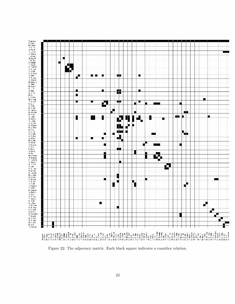
Figure 22: The adjacency matrix. Each black square indicates a coauthor relation.

23

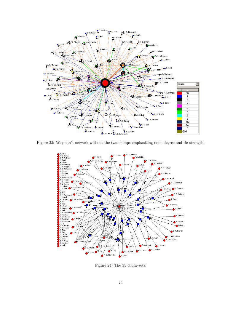
Figure 23: Wegman’s network without the two clumps emphasizing node degree and tie strength.

Figure 24: The 35 clique-sets.

24

Figure 25: The proximity matrix in grey scale; the darker the color the higher the frequency.

25

Figure 26: Random start blockmodel with three clusters using structural equivalence.

26

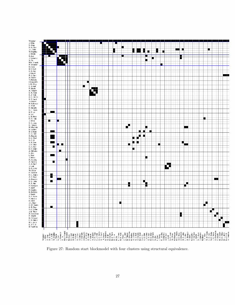
Figure 27: Random start blockmodel with four clusters using structural equivalence.

27

6 Conclusion

There is a potential “elite” group consisting of (Wegman, Solka, W. Martinez, Marchette,and Priebe). Members of this important group are high in degree, closeness and tie strength,removing these vertices will jeopardize the status and connectivity of the network. Structuralholes are yet another characteristic of this ego network.

The analysis presented in this paper suggests that Wegman operates a “mentor” networkwith most of the coauthors being younger than him. Most of them are individuals whoworked with Wegman to establish their future academic/industrial career and then left. Theexception is the elite group, which were already established and have maintained communi-cation up to the present with Wegman.

We can also argue on the quality versus quantity of the publications. Wegman favoredquality of the work rather than quantity. This observation can be concluded by the manycoauthors connected to him with few publications.

Investigating the second level coauthorship network covering at least the elite group is ofimportance, it will provide a more clear and accurate picture of who-wrote-with-who andwhich coauthors are critical to the status of the network. The network is expected to expandand fold into itself. The second-level analysis of Wegman’s network will be the next phase.

Acknowledgement

I would like to express deep gratitude to my advisor Dr. E. Wegman, Dr. M. Tsvetovatand Dr. Y. Said whose guidance, support and advice were very helpful for the successfulcompletion of this project.

References

[1] R. Hanneman and M. Riddle, Introduction to social network methods, Online textbook:http://www.faculty.ucr.edu/∼hanneman/nettext/, Riverside, CA, 2005.

[2] Max Tsvetovat, Social Network Analysis. Lecture 3: Centrality in Social Networks.

[3] V. Batageli W. de Nooy and A. Mrvar, Exploratory social network analysis with pajek,Cambridge University Press, 2004.

[4] S. Wasserman and K. Faust, Social network analysis: Methods and applications, Cam-bridge University Press, New York, 1994.

28