hhs public access longwall gob gas ventholes sequential...

Sequential Gaussian co-simulation of rate decline parameters of longwall gob gas ventholes

C.Özgen Karacana,* and Ricardo A. Oleab

aNIOSH, Office of Mine Safety and Health Research, Pittsburgh, PA, United State

bUSGS, Eastern Energy Resources, Reston, VA, United States

Abstract

Gob gas ventholes (GGVs) are used to control methane inflows into a longwall mining operation

by capturing the gas within the overlying fractured strata before it enters the work environment.

Using geostatistical co-simulation techniques, this paper maps the parameters of their rate decline

behaviors across the study area, a longwall mine in the Northern Appalachian basin. Geostatistical

gas-in-place (GIP) simulations were performed, using data from 64 exploration boreholes, and

GIP data were mapped within the fractured zone of the study area. In addition, methane flowrates

monitored from 10 GGVs were analyzed using decline curve analyses (DCA) techniques to

determine parameters of decline rates. Surface elevation showed the most influence on methane

production from GGVs and thus was used to investigate its relation with DCA parameters using

correlation techniques on normal-scored data. Geostatistical analysis was pursued using sequential

Gaussian co-simulation with surface elevation as the secondary variable and with DCA parameters

as the primary variables. The primary DCA variables were effective percentage decline rate, rate

at production start, rate at the beginning of forecast period, and production end duration. Co-

simulation results were presented to visualize decline parameters at an area-wide scale. Wells

located at lower elevations, i.e., at the bottom of valleys, tend to perform better in terms of their

rate declines compared to those at higher elevations. These results were used to calculate drainage

radii of GGVs using GIP realizations. The calculated drainage radii are close to ones predicted by

pressure transient tests.

Keywords

Sequential Gaussian co-simulation; Geostatistical stochastic simulation; Longwall mining; Gob gas ventholes; Decline curve analysis; Methane control

*Corresponding author. Tel.: +1 412 3864008; fax: +1 412 386 6595. [email protected] (C. Özge Karacan).

Disclaimer: The findings and conclusions in this paper are those of the authors and do not necessarily represent the views of the National Institute for Occupational Safety and Health. Mention of any company name, product, or software does not constitute endorsed by NIOSH or USGS.

Appendix A. Supporting informationSupplementary data associated with this article can be found in the online version at http://dx.doi.org/10.1016/j.ijrmms.2012.11.003.

HHS Public AccessAuthor manuscriptInt J Rock Mech Min Sci (1997). Author manuscript; available in PMC 2015 July 15.

Published in final edited form as:Int J Rock Mech Min Sci (1997). 2013 April ; 59: 1–14.

Author M

anuscriptA

uthor Manuscript

Author M

anuscriptA

uthor Manuscript

http://dx.doi.org/10.1016/j.ijrmms.2012.11.003

1. Introduction

Drilling gob gas ventholes (GGVs) in longwall mining panels is a common technique to

control methane emissions, allowing for the capture of methane within the overlying

fractured strata before it enters the work environment during mining. The usual practice is to

drill the GGVs prior to mining and locate a slotted casing in the zone that is expected to

fracture (fractured zone). As mining advances under the venthole, the strata that surround

the well deform and establish preferential pathways for the released methane, mostly from

the coal seams within the fractured zone, to flow towards the ventholes [1]. The properties

of fractured zones, mainly permeability, are determined through conventional pressure- and

rate-transient well test analyses techniques that are used systematically and routinely for oil

and gas [2–6]. Results showed that permeabilities of bedding plane separations can be as

high as 150 Darcies, with average permeabilities (including fractures and intact formations)

within the slotted casing interval of GGVs varying between 1 Darcy and 10 Darcies [7–9].

GGVs are equipped with exhausters on the surface to provide negative pressure to produce

methane from highly permeable fractured zones with a rate and concentration depending on

various additional factors besides permeability [10–11]. The production life-span of GGVs

may be long or short, depending on mining, borehole drilling, and location as well as

operating conditions, but usually follows a declining trend with time [8] until the exhausters

are shut down as a safety measure against explosion risk, when the methane concentration in

the produced gas decreases to approximately 25%.

It is difficult to predict production performance of GGVs due to the involvement of multiple

factors [10,12]. In addition to complexities given in these studies, boreholes may deform

under mining stresses and strata displacements [13–15], making production predictions even

more difficult. Studies presented in [7,12] do not take borehole stability issues into account

while predicting GGV performance. However, Karacan [10] presented a sensitivity analysis

of variables on total flow rate and methane percentage of gas produced from GGVs. The

sensitivity analyses showed that, when considering the overall performance of GGVs for

methane production rate, the most important variables were 1, whether or not face is

advancing, 2, surface elevation of the venthole (above sea level), 3, overburden, 4, casing

diameter, 5, distance of the venthole to the tailgate, and 6, distance of venthole to panel start.

Multiple factors studied in [10] and then improved in [11] were formulated as a multi-layer-

perceptron (MLP) type neural network to predict GGV production performance. This

module is part of MCP 2.0-Methane Control and Prediction software, v.2 [16] for prediction

and sensitivity analyses purposes. Version 1.3 of this software is briefly discussed [17].

Despite the improvements for understanding the effects of various factors on GGV

production and for predicting GGV performance, there are GGVs that perform much better

or worse than expected in terms of methane production rate and production longevity.

Although these unexpected production behaviors may be due to borehole stability issues, as

mentioned before, they can also be related to spatial location of the borehole and how it

interacts with other important production-influencing factors at that particular position. In

other words, if there is a spatial correlation or stochastic dependency between borehole

Karacan and Olea

Int J Rock Mech Min Sci (1997). Author manuscript; available in PMC 2015 July 15.

Author M

anuscriptA

uthor Manuscript

Author M

anuscriptA

uthor Manuscript

location, its rate transient, and other potentially influencing factors, the analyses should

involve the geographical location of the boreholes, necessitating geostatistical methods.

Geostatistical methods, some of which are described in detail in [18–22], have wide

applications in geology, environmental studies, mining research, and petroleum engineering

[23–28]. More recently, Olea et al. [29] have developed a formulation of a correlated

variables methodology and co-simulation for assessment of gas resources in Woodford shale

play, Arkoma basin, in eastern Oklahoma.

The aim of this paper is to explore the possibility of modeling the attributes of decline curve

analyses (DCA) conducted on gob gas ventholes by taking into account borehole locations

and potential correlations between surface elevations at the wellheads. Geostatistical

stochastic co-simulation methods were used to map the distribution of decline curve

attributes. In addition, cell-based DCA parameters were interpreted with the GIP in the

fractured zone to estimate radii of drainage area of GGVs.

2. Site location and description of area in relation to correlations with gob

gas venthole production

The longwall mining site studied in this paper is in the Pittsburgh coal, Monongahela Group,

southwestern Pennsylvania. The Monongahela Group includes sandstone, siltstone, shale

and commercial coal beds and occurs from the base of the Pittsburgh coal bed to the base of

the Waynesburg coal bed. Thickness within the general study area ranges from 270 to 400 ft.

The Pittsburgh coal seam is unusually continuous and covers more than 5000 square miles

[30], making longwall mining technique highly suitable in this region.

Mining the Pittsburgh seam creates a gas emission zone that extends from the Pittsburgh

Rider to Waynesburg coal beds (Fig. 1), spanning to a height of ~350 ft [31]. However, in

the gas emission zone, Sewickley, Uniontown and Waynesburg coal beds are the main coal

seams that occur within the fractured zone (~ 80–350 ft from the top of the Pittsburgh seam).

During mining, these coal seams are fractured vertically and horizontally and their methane

is liberated into the fracture system. The methane emissions from these coals are believed to

be the main source of gas from the fractured zone, which is controlled by drilling GGVs

from the surface in advance of mining. A simplified stratigraphy of the studied region, a

schematic of a GGV and its drilling distance, the specific panel area where modeling was

conducted, and the monitored GGV locations are shown in Fig. 1.

The GGVs shown in red in Fig. 1 were monitored for flowrates, methane percentage in

produced gas, and pressures at the well head. GGVs shown in blue marks were equipped

with downhole transducers by the field personnel to monitor the change in head of water

initially filled in the boreholes. This information was used to calculate hydraulic

conductivities as a function of face location. Data collected at the surface for flow and

pressures were later used for decline curve analyses.

In southwest Pennsylvania, the topography consists of frequent hills and valleys, which

control underground fracture networks, flow of groundwater, and the presence of gas.

Karacan and Olea


Author M

anuscriptA

uthor Manuscript

Author M

anuscriptA

uthor Manuscript

Fractures are usually within the valleys and are generally stress-relief fractures that were

generated during erosional events [32]. Fracture patterns are vertical, parallel to the valleys

and situated in valley floors.

Wyrick and Borchers [33] reported that groundwater flow associated with stress relief

fractures occurs in the valley bottoms and valley sides. Therefore, wells in the valleys are

more likely to produce high water yields. This fracturing is expected to diminish beneath the

adjacent hills, thereby limiting the effective areal extent and yield of aquifers [32].

Subsidence caused by longwall mining results in tension and compression of the near-

surface zone, increasing or decreasing the fracture transmissibility, especially in valley

bottoms, suggesting that GGVs drilled in the valleys may be more productive [33]. Based on

an earlier integrated study evaluating hydraulic properties of underground strata and their

potential responses to longwall mining, Karacan and Goodman [34] concluded that GGVs

drilled in the valleys might be more productive than those drilled on hilltops. They also

observed that the borehole location affected fracturing during dynamic subsidence in such a

way that hilltop GGVs seemed to fracture earlier than valley-bottom wells. However, the

permeability of the fractures at the hilltop wells was less compared to that of valley-bottom

wells due to greater overburden thickness.

Wells at higher elevations, and thus with greater overburden thickness for a nearly flat coal

bed such as the Pittsburgh seam, usually cause lower hydraulic conductivities and

potentially less effective GGVs as opposed to shallow overburden wells. Thus, less

overburden and lower surface elevations correlate better with GGV production. These

observations and monitoring results are in agreement with Fig. 1 in terms of the influence of

surface elevation on methane production from GGVs, and are the basis for selecting surface

elevation as the secondary variable, as discussed in forthcoming sections.

3. Decline curve analyses of gob gas venthole data

3.1. Production data and analyses methodology

Decline curve analysis is a rate transient test procedure used for analyzing declining

production rates and forecasting future performance of wells. In this paper, Fekete’s rate

transient analysis (RTA) [35] software was used to analyze declining GGV production

performances using both traditional decline approaches and Fetkovich type curves.

In decline curve analysis, it is implicitly assumed that the factors causing the historical

decline continue unchanged during the forecast period. These factors include both reservoir

conditions and operating conditions of the borehole. As long as these conditions do not

change, the trend in decline can be analyzed and extrapolated to forecast future well

performance [35,36]. This implicit assumption can be especially valid for gob reservoirs

after the mining face passes the GGV location by at least several hundreds of feet or after

completion of the panel. At these stages, caving and subsidence are complete at a particular

GGV location, and no further major reservoir changes are expected. Under constant

percentage or exponential decline conditions, plots of log-rate vs. time and rate vs.

cumulative production should both result in straight lines from which the decline rate can be

determined.

Karacan and Olea


Author M

anuscriptA

uthor Manuscript

Author M

anuscriptA

uthor Manuscript

An example of traditional DCA with fitted data of GGV-1 shown in Fig. 1 is given in Fig. 2.

This figure shows the GGV-1 production data analyzed with an exponential decline curve

using gas rate vs. time and gas rate vs. cumulative production plots. Some important data

that can be drawn from these analyses relating to production and forecast intervals, as well

as their locations, are shown schematically in Fig. 3. These parameters and their acronyms,

shown in Fig. 3 caption, will be used as primary variables in co-simulations and will be

referred to frequently in this paper.

The relationship of various parameters in exponential decline analysis are given below for

decline coefficient and cumulative production between two time intervals, respectively,

from the acronyms used in Fig. 3 and its caption:

Cumulative productions at different production times can be obtained by changing the FC to

the desired time in Eq. (2).

3.2. Results of production decline analyses of GGVs

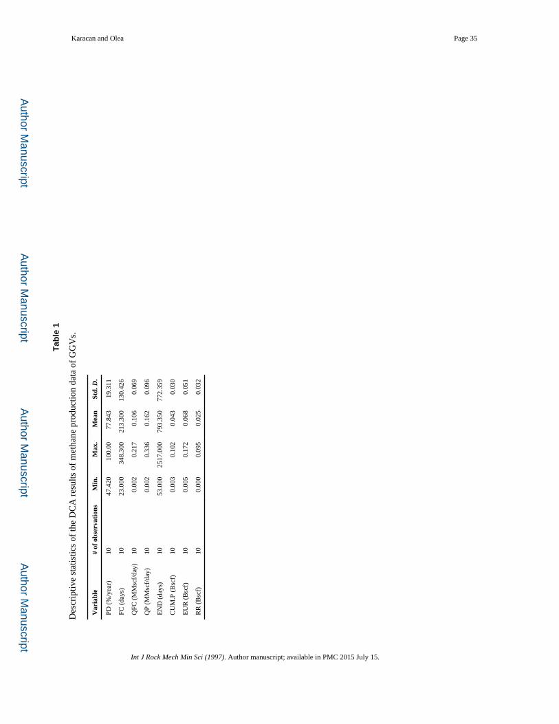
Table 1 shows the descriptive statistics of the DCA results of methane production data. The

DCA allowed for the determination of eight attributes derived from the production of 10

GGVs. These results show that percentage decline of the GGVs ranges from 47 to 100%/

year, with a mean of 78%/year. Table 1 further shows that the rate of methane production at

the start of the GGVs’ production life, just after interception with longwall face, can vary

between low values (~2 Mscf/day) and higher ones (336Mscf/ day). However, the

production can cease at rates between 2 Mscf/ day and 217 Mscf/day (rate at forecast start

period) and the GGVs can be short-lived (23 days) or longer (348.3 days), as observed from

forecast-start time. Depending on their production characteristics, GGVs can capture

cumulative methane between 3 MMscf and 102 MMscf, out of expected ultimate recovery

(EUR) values ranging from 5 MMscf to 172 MMscf. These values correspond to a methane

capture efficiency varying from ~2% to ~60% considering only the minimum and

maximums of EURs. Thus, there are significant differences among the performance of the

GGVs that were drilled in this area.

Ten observations for each DCA attribute are too few to establish a meaningful histogram for

assessing the distributions of the DCA parameters across the study area and for selecting

which ones could be used as primary variables.

4. Surface elevation data and modeling of gas-in-place in fractured zone

The mining district modeled in this work (Fig. 1) hosted Pittsburgh seam panels 1250 ft

wide initially (the first two panels), with wider panels (1450 ft) starting from the 3rd panel.

Karacan and Olea


Author M

anuscriptA

uthor Manuscript

Author M

anuscriptA

uthor Manuscript

Panel lengths were generally 12,000–13,000 ft in length. The dimensions of the area shown

in Fig. 1 are 8624 ft in the y-direction (Northing) and 17,325 ft in the x-direction (Easting).

In this district, overburden depths ranged between 700 and 1000 ft. This area was modeled

in a 100 × 50 (Easting-Northing) Cartesian grid in which each cell was 175 ft in the x-

direction and 176 ft in the y-direction.

Surface elevation of the study area was obtained from U.S. Geological Survey seamless data

warehouse [37] digitally and used as the secondary variable. The original digital resolution

of the surface elevation map of the study area was 30 ft × 30 ft as it was extracted from the

database. However, in order for it to match exactly to the grid model of the study area and to

the GGV locations, the high-resolution data was scaled up to the number of cells and to the

cell dimensions of the model grid using averaging with bi-linear interpolation. Thus, the

final surface elevation map was the same as the above. Fig. 4 shows the up-scaled map,

which was generated for use in GIP calculations and as the secondary variable in co-

simulations.

Fig. 5 shows the histogram of surface elevation data in Fig. 6. Basic statistics in this

histogram, based on the values of 5000 cells, gives a minimum elevation of 932.3 ft, a

maximum elevation of 1384.5 ft, a mean elevation of 1083.6 ft, and a standard deviation of

87.9 ft.

The data used in geostatistical modeling of gas-in-place (GIP) were obtained from 63

vertical exploration boreholes drilled over the mining area shown in Fig. 6. Because the top

of the fractured zone for these mines was 350 ft from the top of the Pittsburgh coal [31], the

data beyond this interval were excluded from further analyses. For each coal seam of interest

in the fractured zone (Sewickley, Uniontown and Waynesburg seams), two attributes were

determined at the spatial locations of each of the exploration boreholes for geostatistical

modeling of GIP: overburden depth and coal thickness. Overburden depths were calculated

by subtracting the sea-level elevation of each of the coal seams from the surface elevation

data at those particular locations. Results of univariate statistical analyses of coal seam

attributes are given in Table 2.

GIP simulations, whose modeling and computational procedure was developed and

documented in detail for a different field in an earlier paper [38] and will not be repeated

here for this district, were still pursued as an independent attribute. The univariate data given

in Table 2 and the spatial distributions of these data based on the exploration boreholes

shown in Fig. 8 are used for geostatistical modeling of GIP. However, GIP has not been

used as a secondary variable in co-simulations simply because surface elevations are

measured and provide more accurate data. In addition, surface elevation was found to be one

of the most influential parameters on GGV production rates and their declines [10].

Nevertheless, GIP data still add value in analyzing performance of GGVs and thus they were

used to compare cumulative productions from GGVs and to set approximate drainage areas

for GGVs after co-simulations.

Karacan and Olea


Author M

anuscriptA

uthor Manuscript

Author M

anuscriptA

uthor Manuscript

4.1. Semivariogram modeling of surface elevation and of GIP attributes

For sequential Gaussian simulation and co-simulation techniques to be applicable, the data

should follow a Gaussian (normal) distribution. Therefore, the surface elevation and

attributes of coals (depth and thickness) were transformed to normal scores by targeting a

Gaussian distribution with a mean of 0 and variance of 1 [20–21]. The semivariograms were

modeled on the normal-score data, and later were transformed back to the original space

during simulations by targeting their original distributions. The Stanford University

Geostatistical Modeling Software (SGeMS) was used for semivariogram analyses and for

geostatistical simulations [20]. The semivariograms were modeled according to the

guidelines provided in [39] and by studying the directional experimental semivariograms of

normal scores. Experimental semivariograms were searched at 0°, 45°, 90°, and 135°

starting from north and changing towards the east direction of lag vectors. In addition, an

omni-directional semivariogram was modeled. Simulations, though, were performed with

the omni-directional semivariograms of each attribute since anisotropy was not detected.

Fig. 7 shows the experimental semivariogram for the normal-score data of Sewickley coal

seam depth and surface elevation as examples of the attributes modeled in this study. The

analytical semivariogram models of the variables for the three coal seams that were used in

GIP calculations are summarized in Table 3.

4.2. Sequential Gaussian simulation of GIP

Sequential Gaussian simulation (SGSIM) is a semivariogram-based simulation technique

that generates simulated results, or so-called realizations, of the attribute in question by

extracting the spatial patterns from the input data and semivariograms. Realizations can be

seen as numerical models of possible distributions of the simulated property in space. In

practice, these realizations take the form of a finite number of simulated maps equally

probable to represent the unknown true map. Therefore, each grid in each of these

realizations, or simulated maps, generates a distribution of the particular attribute. These

distributions can be used to analyze the data statistically for variances and to evaluate the

uncertainty associated with various values in a probabilistic fashion. It should be mentioned

that ordinary kriging and co-kriging could have been used instead of simulation for spatial

modeling. However, kriging causes severe smoothing effect on the results and also

simulation is more suited to evaluate uncertainty [38]. In addition, Heriawan and Koike [40]

compared two spatial models of coal quality by ordinary kriging and sequential Gaussian

simulation, and clarified the merits using the simulation.

In this work, 100 realizations for each attribute of interest for GIP calculations were

generated. For verification of the statistical accuracy of these realizations, the results of

sequential Gaussian simulations of modeled attributes (thickness and overburden depth)

were compared with the original data before proceeding with calculations of GIP and the

associated uncertainties. These comparisons required Q–Q plots of hard data (measured

data) along with SGSIM realizations. Q–Q plots (not shown here but readers are referred to

[38] for an example) gave acceptable linear trends between hard data and realizations,

indicating that the probability distributions of these two datasets are almost the same, and

Karacan and Olea


Author M

anuscriptA

uthor Manuscript

Author M

anuscriptA

uthor Manuscript

SGSIM produces representative simulated distributions of probability distributions of actual

data.

After the representativeness of these realizations for the raw attribute data were checked

using Q–Q plots, GIP computations were performed for each of the three coal seams, which

later were summed to compute the GIP maps of the fractured zone. One hundred realizations

of GIP of the fractured zone for the area shown in Fig. 1 were generated.

The simulation results distributed in each of the realizations can be used for statistical

evaluations of uncertainty using the histograms. For instance, the values of GIP for the

fractured zone can be calculated at 5%, 50%, and 95% quantiles (Q5, Q50, Q95). These

quantiles represent the ranking of the estimated attribute, where each estimated value has the

5th, 50th, and 95th place in ranking analyses. In other words, the estimated values of 5%,

50%, and 95% have a probability to be lower than the actual unknown value. Among these,

Q50 represent the median of the possible population distribution for the calculated variables.

The cell values within each of the 100 realizations and percentile analyses were conducted

to extract the realizations that correspond to Q5, Q50, and Q95 of fractured zone GIP. The

GIP results shows that cumulative GIP in this area ranges between 3550 MMscf (3.55 Bscf)

and 4150 MMscf (4.15 Bscf). These values are important as they state that, assuming GGVs

produce methane only from the GIP in the fractured zone, the cumulative production from

all boreholes combined cannot exceed 4.15 Bscf.

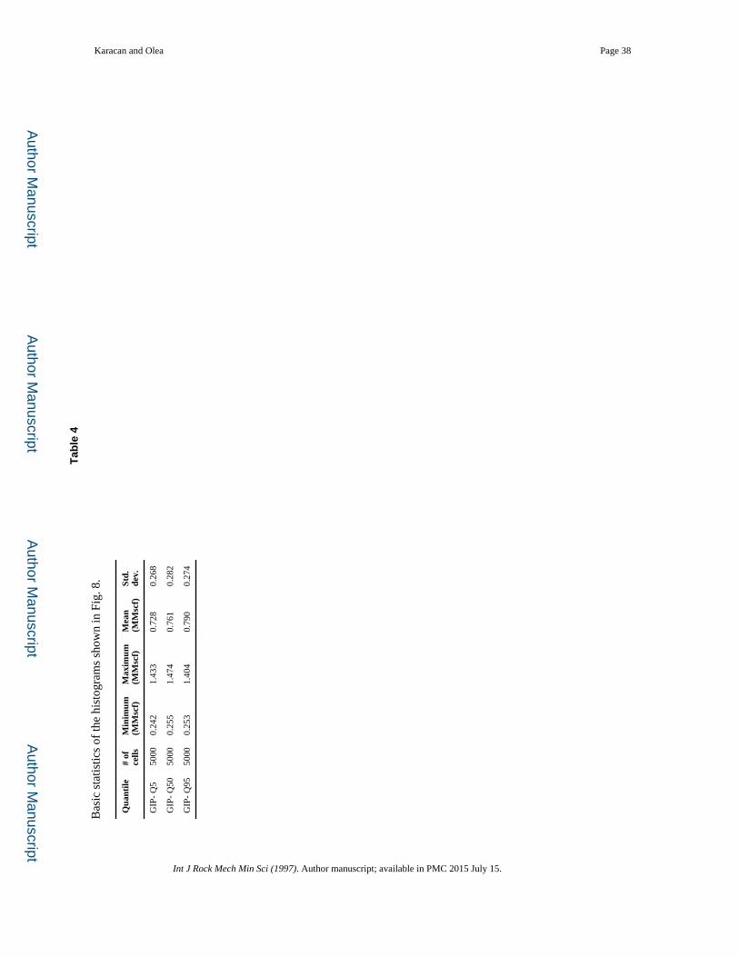
Fig. 8 shows the histograms of cell values (5000 cells) of GIP for Q5, Q50, and Q95, whose

basic statistics are given in Table 4. This figure and table show that the GIP values in

realizations corresponding to Q5, Q50, and Q95 are distributed within a minimum and

maximum range of ~0.24 MMscf/cell and ~1.5 MMscf/cell, respectively, with a mean of

~0.75 MMscf/cell. These values correspond to ~0.34 MMscf/acre, ~2.05 MMscf/acre, and

~1.1 MMscf/acre, as minimum, maximum, and mean, respectively. However, it is also

noteworthy that the histograms given in Fig. 8 show bimodal distributions, which indicate

the existence of two distinct zones of GIP within the study area. GIP maps corresponding to

Q5, Q50, and Q95 (Fig. 9) show that the western portion of the study area has potentially

more GIP in the fractured zone then the eastern portion. Therefore, methane control and

ventilation requirements will be different in these two areas.

5. Selection of primary variables and co-simulations

5.1. Selection of primary variables

In this paper, the potential of geostatistics to model decline curve attributes of a limited

number of GGVs is sought by utilizing the location of wells and by considering the

correlation potential of DCA attributes with surface elevation of wells. For this purpose,

surface elevation data shown in Fig. 4 are used as the secondary variable in co-simulations.

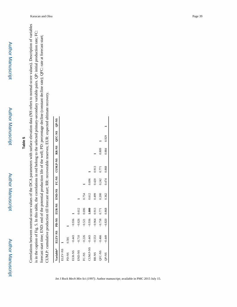
The next step was to identify which DCA parameters could be selected as primary variables

of co-simulations. In order to determine these variables, a correlation analysis between all

possible DCA parameters and surface elevation was conducted using the normal scores of

all attributes. The results of this analysis are given in Table 5. In selecting the primary

Karacan and Olea


Author M

anuscriptA

uthor Manuscript

Author M

anuscriptA

uthor Manuscript

variables based on the correlation coefficients, the objective was to select the meaningful

primary variables that have reasonably high correlations with the secondary variable.

Moreover, two variables having an absolute correlation coefficient larger than 0.9 were

judged dependent upon each other. This excluded the variable RR that had a larger

correlation coefficient with the surface elevation than the variables QFC and QP, for

instance. Additional effort was also made to avoid selecting primary variables that will

repeat themselves in co-simulations. Moreover, selected variables should have enabled

derivation of others using their relations through exponential decline relations given in Eqs.

(1) and (2). Therefore, methane rate at production start (QP), percent decline (PD), end of

possible production period (END), and production rate at start of forecast period (QFC)

were selected as primary variables to be simulated with surface elevation (ELEV).

5.2. Sequential Gaussian co-simulations of primary variables with secondary variables

Different implementations of sequential simulations in SGeMS can be used for different

purposes [20,29]. For this work, sequential Gaussian co-simulation with Markov-model-1

(MM1) was selected. The absence of need to generate cross-correlation, while still

maintaining the ability to produce realistic results [29,41], is an advantage of this method in

the face of especially limited data points.

Sequential Gaussian co-simulation allows for simulation of a Gaussian variable while

accounting for the secondary information to which it correlates [20]. Due to the nature of the

simulation method, the variables should either be Gaussian or should be transformed to

normal scores. The latter was followed in the study since the variables were not Gaussian.

MM1 considers the following Markov-type screening hypothesis during simulations: the

dependence of the secondary variable on the primary is limited to the co-located primary

variable. The cross-covariance is then proportional to the auto-covariance of the primary

variable [20], which can be shown as

where h is the distance vector, C12 is the cross covariance between the two variables, and

C11 is the covariance of primary variable. Thus, solving the co-kriging algorithm with MM1

requires the knowledge of correlation between primary and secondary variables, as well as

the semivariogram(s) of the primary variable(s). These requirements, as implemented in the

face of limited amount of data for primary variables, were addressed by determining the

range of correlation coefficients instead of using a single value. For this purpose, a Monte

Carlo (MC) routine using multi-normal correlation based on Cholesky decomposition was

implemented. The routine generated 1000 normal-score data for each of the primary DCA

variables and the surface elevation by using their normal-score means and standard

deviations. This procedure, implemented for each of the four primary-secondary variable

pairs selected, generated a range of correlation coefficients that were normally distributed

around the 10-data value. These 1000 values were reduced to 100 by random sampling and

were used for running 100 realizations by varying the correlation coefficient in each co-

Karacan and Olea


Author M

anuscriptA

uthor Manuscript

Author M

anuscriptA

uthor Manuscript

simulation run. The correlation coefficient distributions for each primary-secondary variable

pair are given in Fig. 10.

Semivariogram of primary variable based on limited data locations was approximated by the

semivariogram of the secondary variable in normal-score space as all attributes in normal-

score space have sills of 1, regardless of the attribute being modeled. Therefore, the sill of

the semivariogram for surface elevation is the same as the sill of the “unknown”

semivariogram of the primary variable. This is especially true if the primary and the

secondary variables are correlated. This implies that the semivariogram ranges and nuggets

must be quite similar too. Of course, it can be argued that correlation coefficients based on

10 wells are in the order of ~0.7 and thus nugget and ranges may not be exactly the same.

This argument is partly taken care of by generating a range of correlation coefficients

around the mean that will reflect on results and is also supported by the influence of surface

elevation on production and decline characteristics discussed in [10,34]. Thus, as

continuation of the above approach approximating the parameters of the primary

semivariogram, the same shape of the secondary semivariogram, which is given in Fig. 7B,

was used as the primary semivariogram. As the last step in simulation methodology, the

normal-score primary attributes generated from co-simulations were back-transformed into

real-space values.

6. Results and discussion

6.1. Co-simulated realizations of primary variables using cell-based evaluation

Co-simulations using the MM1 approach were performed to generate 100 realizations for

each of the primary variables. The realizations of DCA parameters co-simulated with

surface elevation shown in Fig. 4 can be used in a variety of ways to improve the

understanding of rate decline properties of GGVs drilled at different locations. One of the

most useful applications of all 100 realizations from each of the parameters is to calculate

local probability above certain thresholds. With this application, local probability at each

cell location can be calculated using the threshold value and the local cumulative probability

distribution from 100 values. The results are presented as probability maps. In this study, the

median values of each of the co-simulated DCA parameters were selected as the threshold

value for local probability calculations. The median values were 77.8%/year for PD, 787.8

days for END, 0.106 MMscf/day for QFC, and 0.163 MMscf/day for QP. The maps that

show the local probabilities for these four DCA parameters to have values above their

medians are shown in Fig. 11A–D.

The local probability maps were generated based on 100 values in each of the 5000 cells

and, comparing these with the surface elevation map given in Fig. 6, show general areas

where GGVs perform above the set threshold values (medians). These figures show that the

probability of percentage decline being larger than 77.8%/year is greater at high elevations

(Fig. 11A) and that the GGVs drilled at or close to hilltops can have very high decline rates

over time and may not produce for long enough periods to extract an incremental amount of

methane. This is also confirmed with the probability map given in Fig. 11B, which indicates

that hilltop wells have very little probability producing with extended periods of time

(exceeding ~788 days). These maps show that only the GGVs drilled at the lowest

Karacan and Olea


Author M

anuscriptA

uthor Manuscript

Author M

anuscriptA

uthor Manuscript

elevations have high probabilities of having slower decline rates and extended production

lives.

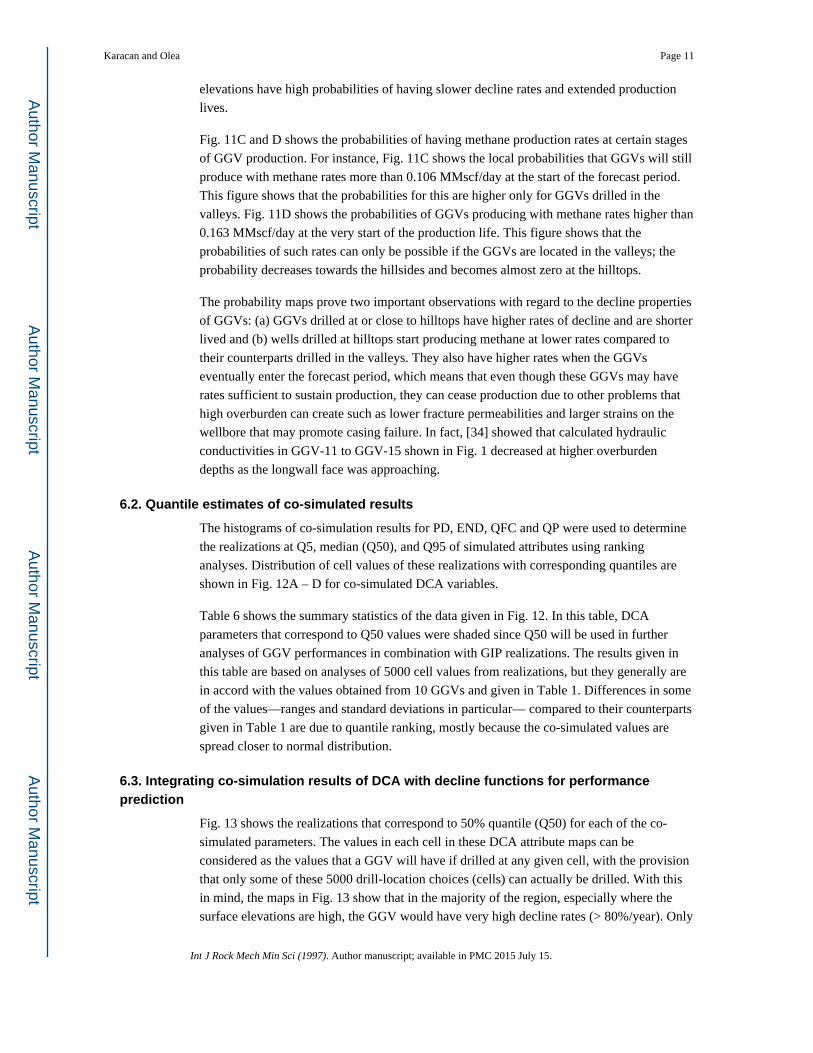
Fig. 11C and D shows the probabilities of having methane production rates at certain stages

of GGV production. For instance, Fig. 11C shows the local probabilities that GGVs will still

produce with methane rates more than 0.106 MMscf/day at the start of the forecast period.

This figure shows that the probabilities for this are higher only for GGVs drilled in the

valleys. Fig. 11D shows the probabilities of GGVs producing with methane rates higher than

0.163 MMscf/day at the very start of the production life. This figure shows that the

probabilities of such rates can only be possible if the GGVs are located in the valleys; the

probability decreases towards the hillsides and becomes almost zero at the hilltops.

The probability maps prove two important observations with regard to the decline properties

of GGVs: (a) GGVs drilled at or close to hilltops have higher rates of decline and are shorter

lived and (b) wells drilled at hilltops start producing methane at lower rates compared to

their counterparts drilled in the valleys. They also have higher rates when the GGVs

eventually enter the forecast period, which means that even though these GGVs may have

rates sufficient to sustain production, they can cease production due to other problems that

high overburden can create such as lower fracture permeabilities and larger strains on the

wellbore that may promote casing failure. In fact, [34] showed that calculated hydraulic

conductivities in GGV-11 to GGV-15 shown in Fig. 1 decreased at higher overburden

depths as the longwall face was approaching.

6.2. Quantile estimates of co-simulated results

The histograms of co-simulation results for PD, END, QFC and QP were used to determine

the realizations at Q5, median (Q50), and Q95 of simulated attributes using ranking

analyses. Distribution of cell values of these realizations with corresponding quantiles are

shown in Fig. 12A – D for co-simulated DCA variables.

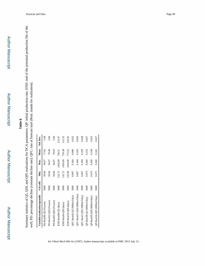
Table 6 shows the summary statistics of the data given in Fig. 12. In this table, DCA

parameters that correspond to Q50 values were shaded since Q50 will be used in further

analyses of GGV performances in combination with GIP realizations. The results given in

this table are based on analyses of 5000 cell values from realizations, but they generally are

in accord with the values obtained from 10 GGVs and given in Table 1. Differences in some

of the values—ranges and standard deviations in particular— compared to their counterparts

given in Table 1 are due to quantile ranking, mostly because the co-simulated values are

spread closer to normal distribution.

6.3. Integrating co-simulation results of DCA with decline functions for performance prediction

Fig. 13 shows the realizations that correspond to 50% quantile (Q50) for each of the co-

simulated parameters. The values in each cell in these DCA attribute maps can be

considered as the values that a GGV will have if drilled at any given cell, with the provision

that only some of these 5000 drill-location choices (cells) can actually be drilled. With this

in mind, the maps in Fig. 13 show that in the majority of the region, especially where the

surface elevations are high, the GGV would have very high decline rates (> 80%/year). Only

Karacan and Olea


Author M

anuscriptA

uthor Manuscript

Author M

anuscriptA

uthor Manuscript

in the regions where there are valleys would the GGVs have decline rates in the 50–70%/

year range. In addition, these high decline rates would be associated with lower methane

production rates at the start of GGV production. The values presented based on the Q50

maps of DCA attributes in Fig. 13 are in agreement with the local probabilities calculated

for each cell (Fig. 11) and the interpretation offered in Section 6.1.

The spatial DCA data given as maps not only can be used to generate synthetic decline

curve analysis test data for selected locations but can also be used to predict performance of

any GGV that can be drilled at any random location on the terrain by use of decline

functions. As an example of this application, the virtual GGVs shown in Fig. 14 were

created and located randomly at various locations on the surface elevation map to cover a

range of surface elevations and locations on the terrain, such as valleys, hillsides and

hilltops. By using the DCA maps from co-simulations as the decline parameters of these

GGVs, and by using Eq. 2 as the expression for cumulative production in exponentially

declining wells at any given time, realizations of cumulative methane productions were

created. These calculations were performed by replacing FC (forecast start time) term in Eq.

2 with desired times; 30, 60, 120, 180, and 240 days, in this case. Then, a ranking analysis

was performed on the results to find the realizations that corresponded to various quantiles,

using the same procedure described in Section 6.2 to find various quantiles of DCA

simulations. To finish the prediction for cumulative methane productions, the data at the

exact locations of the virtual GGVs were extracted. These data from Q50 realizations of 30,

60, 90, 120, 180, and 240 days are given in Fig. 15.

Fig. 15 shows that the GGVs had differing production performances based on the DCA data

that these GGVs acquired at their locations. The cumulative production data predicted for

various production times showed that the GGVs located at the highest elevations, such as

hilltops (E, F, G, I, K), had generally the lowest amount of cumulative methane production.

On the other hand, the GGVs located at the lowest elevations (C, D, H, J, L), such as valleys

and lower edge of the hills, had the highest cumulative methane productions. The difference

in cumulative production between best and worst performing GGVs at the end of 240 days

was about 15 MMscf of methane.

6.4. Integrating performance prediction based on DCA maps with GIP results to estimate drainage area

GGVs, as with other boreholes in any reservoir, should be drilled with a well-planning

protocol to determine where and how many wellbores should be drilled in a given region by

considering surface and reservoir conditions. This includes paying attention to any possible

interference between GGVs. The results presented in the previous section can be integrated

with GIP maps (Fig. 9) to estimate possible drainage radii of GGVs in the fractured zone

and potential for interference due to overlapping drainage zones.

In order to demonstrate the drainage radius estimation for GGVs, the same virtual GGVs

shown in Fig. 14 and their performance results given in Fig. 15 were used. These results

were also combined with the GIP maps given in Fig. 9. The GIP amounts at the exact same

cells as the virtual GGVs are shown in Fig. 16 for Q5, Q50, and Q95. This figure shows that

GIP is lowest at A, C, and D locations and the amount is ~0.4 MMscf/cell. GIP is highest at

Karacan and Olea


Author M

anuscriptA

uthor Manuscript

Author M

anuscriptA

uthor Manuscript

B, E, F, I, K, and L. These are primarily the locations towards the west and south of the

model area. GIP amount in these locations is between 0.8 and 1.2 MMscf/cell range.

Estimation of the drainage radii of GGVs starts with evaluating cumulative methane

production of GGVs at any given time. For this purpose, cumulative production data for 30

days and 240 days at 50% quantile (Q50) given in Fig. 15 were used, as well as the Q50

values of the GIP at given locations from Fig. 16. Knowing the size of each cell, the

cumulative production amount, and the GIP corresponding to each location, the drainage

radius of each GGV can be calculated. However, this calculation is based on the assumption

that all GIP will be produced from the GGV and surrounding cells, i.e., recovery efficiency

is 100%. Based on this procedure, the estimated drainage radii of each GGV are given in

Fig. 17 as a function of surface elevation at virtual GGV locations. This figure shows that

drainage radii can change between 200 and 400 ft at only 30 days of production of GGVs,

whereas they increase to values between 500 ft and 1000 ft, depending on the location and

the GIP values, after 240 days of production. If different methane extraction efficiency is

taken into account, the estimated radii will change accordingly. Also, it is clearly seen from

this plot that drainage radii decrease with increase in surface elevation of the GGV location.

This is in agreement with the impact of surface elevation on DCA parameters discussed

earlier in this paper and in [10].

Radii values estimated in this section compare favorably with the ones predicted from

pressure transient tests. Karacan [7] predicted radii of investigations for operating GGVs as

578 and 2818 ft, depending on the locations, by use of pressure transient analyses of multi-

rate drawdown test techniques. The results given in this paper also compare, within the order

of magnitude, with the radius of investigation (~4000 ft) of a well in a completely different

setting and known to produce from a bedding-plane separation [9] in a bounded gob

reservoir.

The differences in production behaviors and rate transient (decline) behaviors of gob gas

ventholes, along with their radii of investigations, can be attributed to various factors as

discussed previously. Surface elevation of drill locations can have significant correlations

with rate transient behaviors of these wells. Analyses reveal that the better performing wells

are usually at lower elevations (and lower overburden depths) compared to poorly

performing ones. Therefore, locations of the GGVs should be selected with care. This can be

attributed to higher fracture permeability and shorter casing length for the exhauster to pull

the methane, as opposed to tighter fractures below hilltops and longer casings. Therefore, if

the GGVs have to be drilled at hilltops, it is advisable to drill them at closer spacings due to

the smaller radius of drainage that was proven in this study and in earlier studies. The

drainage radii can also be estimated using DCA and GIP predictions, which will give better

design criteria when considered together. Along these lines, geostatistical simulation and co-

simulation techniques can be used as advanced tools as part of the planning and to assess

uncertainty in making the decisions related to drilling locations and prediction of rate

declines of the GGVs.

Here we have simulated all four primary variables by correlating them to the same

secondary variable. A challenge for the future that should yield additional improvements

Karacan and Olea


Author M

anuscriptA

uthor Manuscript

Author M

anuscriptA

uthor Manuscript

would be the simultaneous simulation of all five attributes. In addition, a rock fracture

network model of gob and geostatistical implementation of fractures to compare and

improve accuracy of the findings of simulation of DCA parameters will be highly valuable.

Such models can show the paths of fluid flow through rock fractures [42,43] and improve

the understanding on DCA parameters.

7. Summary and conclusions

In this paper, geostatistical analysis was pursued using sequential Gaussian co-simulation to

characterize decline curve analyses (DCA) of gob gas ventholes in combination with GIP in

fractured zone and surface elevation. Surface elevation was selected as the secondary

variable, while various attributes of DCA were treated as primary variables. GIP was also

simulated with sequential Gaussian technique, used in conjunction with decline curve results

to determine the drainage radii and production quantities.

The results obtained from this study evaluated important attributes of methane capture from

mining environments, such as gob gas venthole production rates, decline rates, production

ending durations, and cumulative gas productions. Employing sequential Gaussian

simulation and co-simulation enabled not only the estimation of important parameters of

DCA that have correlations with surface elevations but also the assessment of their

uncertainty and values at certain quantiles of statistical evaluation.

This study showed that GGVs can have very high decline rates for a majority of the modeled

mining district. In addition, these high decline rates were associated with lower production

rates at the start of production and consequently less cumulative production. Geostatistical

simulation results were used to calculate drainage radii of GGVs using GIP realizations.

This work showed that the calculated drainage radii were close to ones predicted by pressure

transient tests. Therefore, geostatistical analyses along with co-simulations of DCA and GIP

and surface elevation data could be used to estimate the rate transient parameters and

drainage radii of the wellbores, thus aiding designers in both placement and spacing of the

GGVs.

Although the general belief in the coal region of the Northern Appalachian Basin is that gas

production is improved by drilling GGVs at the margins of the tailgate in the longwall panel,

this study showed that surface elevation might be an important consideration as well.

Therefore, it is important to select the locations of the GGVs with care. In general, wells

located at lower elevations, i.e., at the bottom of valleys, tended to perform better in terms of

their rate declines compared to those at higher elevations. Thus, it is advisable to drill GGVs

with closer spacing at hilltops due to their smaller radii of investigations.

In conclusion, geostatistical simulation and co-simulation techniques can be used as

advanced tools as part of the planning process and to assess uncertainty in making decisions

related to drilling locations and prediction of rate declines of the GGVs.

Conversion table (English to SI units)

1 ft = 0.3048 m

Karacan and Olea


Author M

anuscriptA

uthor Manuscript

Author M

anuscriptA

uthor Manuscript

1 ft2 = 22.957 × 10−6 acre

1 MMscf = 28316 m3

1 scfm = 0.0004719 m3/s

Supplementary Material

Refer to Web version on PubMed Central for supplementary material.

Acknowledgments

We are grateful for the reviews as part of the internal approval process by our institutions: Gerrit Goodman on the NIOSH side, and Leslie F. Ruppert (USGS) and Michael Ed. Hohn (West Virginia Geological and Economic Survey) for the U.S. Geological Survey. We also thank Chris Garrity (U.S. Geological Survey) for providing the high-resolution surface elevation data.

References

1. Karacan CÖ, Esterhuizen GS, Schatzel S, Diamond WP. Reservoir-simulation based modeling for characterizing longwall methane emissions and gob gas venthole production. Int J Coal Geol. 2007; 71:225–245.

2. Nashawi IS. Pressure transient analysis of infinite-conductivity fractured wells producing at high flow rates. J Petrol Sci Eng. 2008; 63:73–83.

3. Sheng JJ. A new technique to determine horizontal and vertical permeabilities from the time-delayed response of a vertical interference test. Transp Porous Media. 2009; 77:507–527.

4. Escobar FH, Ibagon OE, Montealegre MM. Average reservoir pressure determination for homogeneous and naturally fractured formations from multi-rate testing with the TDS technique. J Petrol Sci Eng. 2007; 99:204–212.

5. King GR, Ertekin T, Schwerer FC. Numerical simulation of the transient behavior of coal-seam degasification wells. SPE Form Eval. 1986:165–183.

6. Kuchuk FJ, Onur M. Estimating permeability distribution from 3 D interval pressure transient tests. J Petrol Sci Eng. 2003; 39:5–27.

7. Karacan CÖ. Reconciling longwall gob gas reservoirs and venthole production performances using multiple rate drawdown well test analysis. Int J Coal Geol. 2009; 80:181–195.

8. Dougherty HN, Karacan CÖ, Goodman GVR. Reservoir diagnosis of longwall gobs through drawdown tests and decline curve analyses of gob gas venthole productions. Int J Rock Mech Min Sci. 2010; 47:851–857.

9. Karacan CÖ, Goodman GVR. Monte Carlo simulation and well testing applied in evaluating reservoir properties in a deforming longwall overburden. Transp Porous Media. 2011; 86:415–434.

10. Karacan CÖ. Forecasting gob gas venthole production performances using intelligent computing methods for optimum methane control in longwall coal mines. Int J Coal Geol. 2009; 79:131–144.

11. Karacan CÖ, Luxbacher KD. Stochastic modeling of gob gas venthole production performances in active and completed longwall coal mines. Int J Coal Geol. 2010; 84:125–140.

12. Lunarzewski LW. Gas emission prediction and recovery in underground coal mines. Int J Coal Geol. 1998; 35:117–145.

13. Whittles DN, Lowndes IS, Kingmana SW, Yates C, Jobling S. Influence of geotechnical factors on gas flow experienced in a UK longwall coal mine panel. Int J Rock Mech Min Sci. 2006; 43:369–387.

14. Whittles DN, Lowndes IS, Kingman SW, Jobling Yates CS. The stability of methane capture boreholes around a long wall coal panel. Int J Coal Geol. 2007; 71:313–328.

15. Karacan CÖ, Ruiz FA, Cote M, Phipps S. Coal mine methane: a review of capture and utilization practices with benefits to mining safety and to greenhouse gas reduction. Int J Coal Geol. 2011; 86:121–156.

Karacan and Olea


Author M

anuscriptA

uthor Manuscript

Author M

anuscriptA

uthor Manuscript

16. Karacan, CÖ. Methane control and prediction (MCP) software (version 2.0). 2010. <http://www.cdc.gov/niosh/mining/products/product180.htm>

17. Dougherty HN, Karacan CÖ. A new methane control and prediction software suite for longwall mines. Comput Geosci. 2011; 37:1490–1500.

18. Deutsch, CV.; Journel, AG. GSLIB Geostatistical software library and user’s guide. 2nd edition. New York: Oxford University Press; 1998.

19. Gómez-Hernández, JJ.; Cassiraga, EF. Theory and practice of sequential simulation. In: Armstrong, M.; Dowd, PA., editors. Geostatistical simulation. Dordrecht: Kluwer; 1994. p. 111-124.

20. Remy, N.; Boucher, A.; Wu, J. Applied geostatistics with SGeMS, a user’s guide. Cambridge: Cambridge University Press; 2009.

21. Olea, RA. A Practical primer on geostatistics. U.S. Department of the Interior. U.S. Geological Survey, Open-File Report 2009-1103; 2009.

22. Wackernagel, H. Multivariate geostatistics—an introduction with applications. 3rd edition. Berlin: Springer; 2010.

23. Hohn ME, Neal DW. Geostatistical analysis of gas potential in Devonian shales of West Virginia. Comput Geosci. 1986; 12:611–617.

24. Watson WD, Ruppert LF, Bragg LJ, Tewalt SJ. A geostatistical approach to predicting sulfur content in the Pittsburgh coal bed. Int J Coal Geol. 2001; 48:1–22.

25. Carroll ZL, Oliver MA. Exploring the spatial relations between soil physical properties and apparent electrical conductivity. Geoderma. 2005; 128:354–374.

26. Heriawan MN, Koike L. Identifying spatial heterogeneity of coal resource quality in a multilayer coal deposit by multivariate geostatistics. Int J Coal Geol. 2008; 73:307–330.

27. Hindistan MA, Tercan AE, Unver B. Geostatistical coal quality control in longwall mining. Int J Coal Geol. 2010; 81:139–150.

28. Olea RA, Luppens JA, Tewalt SJ. Methodology for quantifying uncertainty in coal assessments with an application to a Texas lignite deposit. Int J Coal Geol. 2011; 85:78–90.

29. Olea RA, Houseknecht DW, Garrity CP, Cook TA. Formulation of a correlated variables methodology for assessment of continuous gas resources with application to the Woodford play, Arkoma Basin, eastern Oklahoma. Bol Geol Min. 2011; 122:483–496.

30. Tewalt, SJ.; Ruppert, LF.; Bragg, LJ.; Carlton, RW.; Brezinski, DK.; Wallack, RN.; Butler, DT. 2000 Resource assessment of selected coal beds and zones in the Northern and Central Appalachian Basin Coal Regions, by the Northern and Central Appalachian Basin Coal Regions Assessment Team. U.S. Geological Survey Professional Paper 1625-C; 2001. p. 101[Chapter C].

31. Karacan, CÖ. Goodman GVR Probabilistic modeling using bivariate normal distributions for identification of flow and displacement intervals in longwall overburden. Int J Rock Mech Min Sci. 2011; 48:27–41.

32. Stoner, J.; Williams, DR.; Buckwalter, TF.; Felbinger, JK.; Pattison, KL. Water resources and the effects of coal mining, Greene County, Pennsylvania. Pennsylvania: Water Resource Report 63; 1987.

33. Wyrick, GG.; Borchers, JW. Hydrologic effects of stress relief fracturing in an Appalachian valley. Washington DC: US Department of the Interior, US Geological Survey, Water Supply Paper 2177; 1981.

34. Karacan CÖ, Goodman GVR. Hydraulic conductivity changes and influencing factors in longwall overburden determined by slug tests in gob gas ventholes. Int J Rock Mech Min Sci. 2009; 46:1162–1174.

35. Fekete Associates. F.A.S.T. RTA. Advanced rate transient analysis. Calgary, Alberta: 2010. <http://www.fekete.com/software/rta/description.asp>

36. Dake, LP. Fundamentals of reservoir engineering. Amsterdam: Elsevier; 1978.

37. USGS. Seamless Data Warehouse. Data available from U.S. Geological Survey, Earth Resources Observation and Science (EROS) Center, Sioux Falls, SD. 2011. <http://seamless.usgs.gov/faq_listing.php?id=1>

Karacan and Olea


Author M

anuscriptA

uthor Manuscript

Author M

anuscriptA

uthor Manuscript

http://www.cdc.gov/niosh/mining/products/product180.htm

http://www.cdc.gov/niosh/mining/products/product180.htm

http://www.fekete.com/software/rta/description.asp

http://seamless.usgs.gov/faq_listing.php?id=1

http://seamless.usgs.gov/faq_listing.php?id=1

38. Karacan CÖ, Olea RA, Goodman GVR. Geostatistical modeling of gas emission zone and its in-place gas content for Pittsburgh seam mines using sequential Gaussian simulations. Int J Coal Geol. 2012; 90–91:50–71.

39. Olea RA. A six-step practical approach to semivariogram modeling. Stochastic Environ Res Risk Assess. 2006; 20:307–318.

40. Heriawan MN, Koike K. Uncertainty assessment of coal tonnage by spatial modeling of seam distribution and coal quality. Int J Coal Geol. 2008; 76:217–226.

41. Karacan, CÖ. Goodman GVR Analyses of geological and hydrodynamic controls on methane emissions experienced in a Lower Kittanning coal mine. Int J Coal Geol. 2012; 98:110–127.

42. Xu C, Dowd P. A new computer code for discrete fracture network modeling. Comput Geosci. 2010; 36:292–301.

43. Koike K, Sanga T. Incorporation of fracture directions into 3D geostatistical methods for a rock fracture system. Environ Earth Sci. 2012; 66:1403–1414.

Karacan and Olea


Author M

anuscriptA

uthor Manuscript

Author M

anuscriptA

uthor Manuscript

Fig. 1. Schematic representation of stratigraphy and completion of the gob gas ventholes (GGVs),

as well as panels and locations of the GGVs, in the study area. The dimensions of the area

shown in this figure are 8624 ft in the y-direction and 17,325 ft in the x-direction. (For

interpretation of the references to color in this figure caption, the reader is referred to the

web version of this article.)

Karacan and Olea


Author M

anuscriptA

uthor Manuscript

Author M

anuscriptA

uthor Manuscript

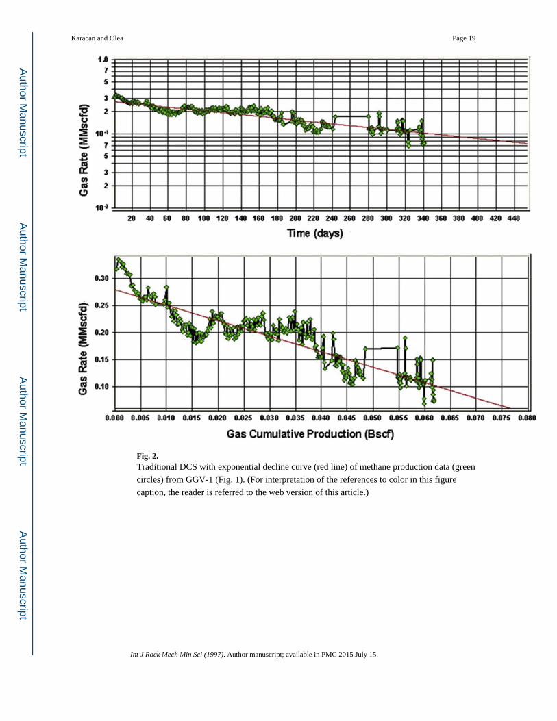
Fig. 2. Traditional DCS with exponential decline curve (red line) of methane production data (green

circles) from GGV-1 (Fig. 1). (For interpretation of the references to color in this figure

caption, the reader is referred to the web version of this article.)

Karacan and Olea


Author M

anuscriptA

uthor Manuscript

Author M

anuscriptA

uthor Manuscript

Fig. 3. Schematic representation of rate parameters and important times in exponential decline

analysis. In this plot, QP, initial production rate; TP, production start time; FC, forecast start

time; END, end of the potential production life of the well; PD, percentage decline (constant

decline rate); QFC, rate at forecast start; CUM.P, cumulative production till forecast start;

RR, recoverable reserves; EUR, expected ultimate recovery; Qab, abandonment rate.

Karacan and Olea


Author M

anuscriptA

uthor Manuscript

Author M

anuscriptA

uthor Manuscript

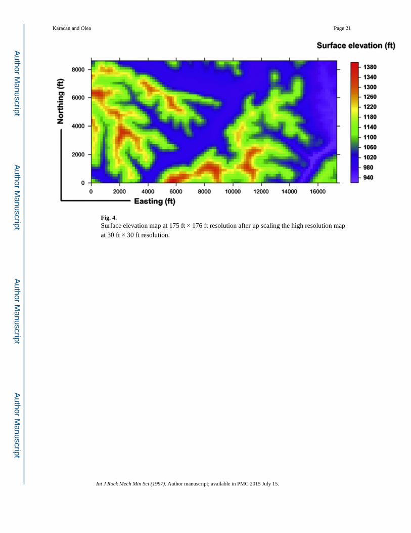
Fig. 4. Surface elevation map at 175 ft × 176 ft resolution after up scaling the high resolution map

at 30 ft × 30 ft resolution.

Karacan and Olea


Author M

anuscriptA

uthor Manuscript

Author M

anuscriptA

uthor Manuscript

Fig. 5. Histograms of the surface elevation data shown in Fig. 4 and its normal score distribution.

Karacan and Olea


Author M

anuscriptA

uthor Manuscript

Author M

anuscriptA

uthor Manuscript

Fig. 6. Spatial locations of the exploration boreholes drilled over the area shown in Fig. 1.

Karacan and Olea


Author M

anuscriptA

uthor Manuscript

Author M

anuscriptA

uthor Manuscript

Fig. 7. Omni-directional experimental semivariograms of normal scores of Sewickley seam depth

(A) and surface elevation (B) (red crosses), and the spherical analytical semivariograms

modeling them (black line). (For interpretation of the references to color in this figure

caption, the reader is referred to the web version of this article.)

Karacan and Olea


Author M

anuscriptA

uthor Manuscript

Author M

anuscriptA

uthor Manuscript

Fig. 8. Distributions of fractured zone GIP in realizations corresponding to quantiles Q5, Q50 and

Q95 (Real stands for realization in the legend).

Karacan and Olea


Author M

anuscriptA

uthor Manuscript

Author M

anuscriptA

uthor Manuscript

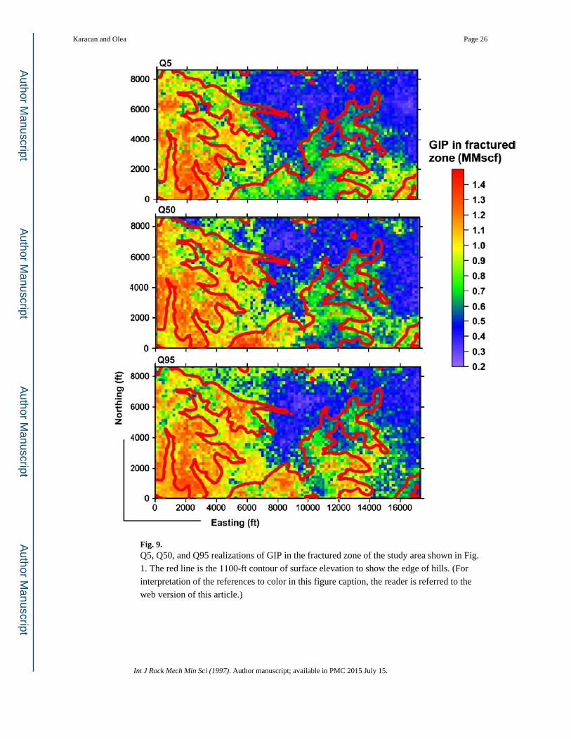
Fig. 9. Q5, Q50, and Q95 realizations of GIP in the fractured zone of the study area shown in Fig.

1. The red line is the 1100-ft contour of surface elevation to show the edge of hills. (For

interpretation of the references to color in this figure caption, the reader is referred to the

web version of this article.)

Karacan and Olea


Author M

anuscriptA

uthor Manuscript

Author M

anuscriptA

uthor Manuscript

Fig. 10. Range of correlation coefficients generated for each of the primary-secondary variable pairs

to be used in co-simulations.

Karacan and Olea


Author M

anuscriptA

uthor Manuscript

Author M

anuscriptA

uthor Manuscript

Fig. 11. Maps that show the local probabilities for DCA parameters for values above their medians.

The red line is the 1100-ft surface elevation contour. (For interpretation of the references to

color in this figure caption, the reader is referred to the web version of this article.)

Karacan and Olea


Author M

anuscriptA

uthor Manuscript

Author M

anuscriptA

uthor Manuscript

Fig. 12. Histograms of cell values in realizations corresponding to Q5, Q50, and Q95 of DCA

parameters (real stands for realization in the legends).

Karacan and Olea


Author M

anuscriptA

uthor Manuscript

Author M

anuscriptA

uthor Manuscript

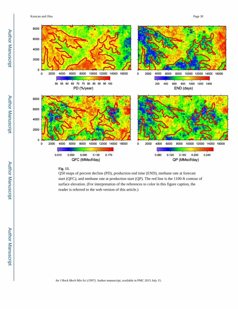
Fig. 13. Q50 maps of percent decline (PD), production end time (END), methane rate at forecast

start (QFC), and methane rate at production start (QP). The red line is the 1100-ft contour of

surface elevation. (For interpretation of the references to color in this figure caption, the

reader is referred to the web version of this article.)

Karacan and Olea


Author M

anuscriptA

uthor Manuscript

Author M

anuscriptA

uthor Manuscript

Fig. 14. Virtual GGV locations to predict their performances.

Karacan and Olea


Author M

anuscriptA

uthor Manuscript

Author M

anuscriptA

uthor Manuscript

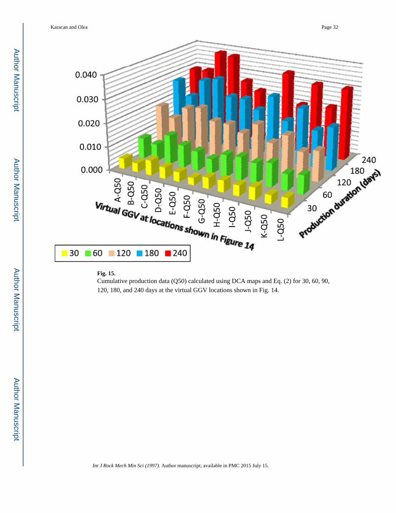
Fig. 15. Cumulative production data (Q50) calculated using DCA maps and Eq. (2) for 30, 60, 90,

120, 180, and 240 days at the virtual GGV locations shown in Fig. 14.

Karacan and Olea


Author M

anuscriptA

uthor Manuscript

Author M

anuscriptA

uthor Manuscript

Fig. 16. GIP amounts determined from Q5, Q50 and Q95 realizations for GGV locations shown in

Fig. 14.

Karacan and Olea


Author M

anuscriptA

uthor Manuscript

Author M

anuscriptA

uthor Manuscript

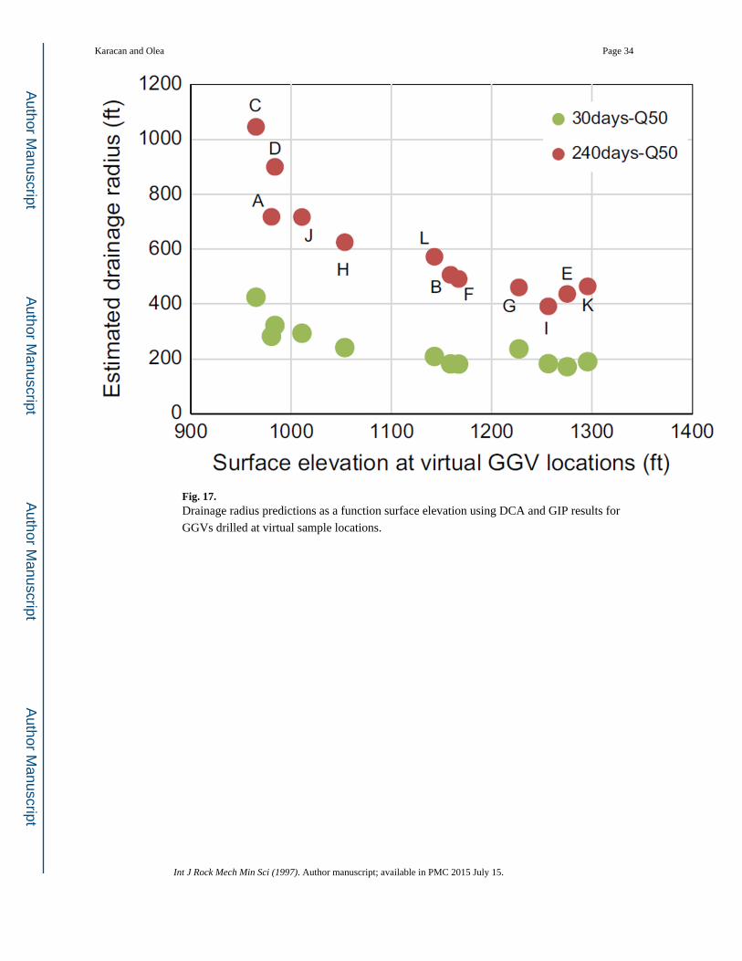
Fig. 17. Drainage radius predictions as a function surface elevation using DCA and GIP results for

GGVs drilled at virtual sample locations.

Karacan and Olea


Author M

anuscriptA

uthor Manuscript

Author M

anuscriptA

uthor Manuscript

Author M

anuscriptA

uthor Manuscript

Author M

anuscriptA

uthor Manuscript

Karacan and Olea

Tab

le 1

Des

crip

tive

stat

istic

s of

the

DC

A r

esul

ts o

f m

etha

ne p

rodu

ctio

n da

ta o

f G

GV

s.

Var

iabl

e#

of o

bser

vati

ons

Min

.M

ax.

Mea

nSt

d. D

.

PD (

%/y

ear)

1047

.420

100.

0077

.843

19.3

11

FC (

days

)10

23.0

0034

8.30

021

3.30

013

0.42

6

QFC

(M

Msc

f/da

y)10

0.00

20.

217

0.10

60.

069

QP

(MM

scf/

day)

100.

002

0.33

60.

162

0.09

6

EN

D (

days

)10

53.0

0025

17.0

0079

3.35

077

2.35

9

CU

M.P

(B

scf)

100.

003

0.10

20.

043

0.03

0

EU

R (

Bsc

f)10

0.00

50.

172

0.06

80.

051

RR

(B

scf)

100.

000

0.09

50.

025

0.03

2


Author M

anuscriptA

uthor Manuscript

Author M

anuscriptA

uthor Manuscript

Karacan and Olea

Table 2

Univariate statistical parameters of depth and thickness encountered by the exploration boreholes for

Sewickley, Uniontown and Waynesburg coal seams.

Depth (ft) Sewickley Uniontown Waynesburg

# of data 62 30 63

Mean 580.73 405.97 346.14

St. dev. 130.62 139.44 127.47

Variance 17,061.35 19,443.67 16,247.78

Minimum 341.73 192.70 103.60

Maximum 803.79 641.00 569.15

Thickness (ft)

# of data 62 30 63

Mean 3.50 0.27 5.37

St. Dev. 1.994 0.088 0.585

Variance 3.979 0.008 0.343

Minimum 0.33 0.10 3.60

Maximum 6.90 0.50 6.99


Author M

anuscriptA

uthor Manuscript

Author M

anuscriptA

uthor Manuscript

Karacan and Olea

Table 3

Summary of parameters that describe analytical semivariograms for depth and thickness attributes of

Sewickley, Uniontown and Waynesburg coal seams, which were used to calculate GIP, and surface elevation.

All semivariograms were analyzed using normal-score data and described with one-nested structure (model).

Depth (ft) Sewickley (SWC) Uniontown coal (UNC) Waynesburg (WBC) Exploration boreholes

Model Spherical Exponential Exponential

Nugget 0.1 0.1 0.1

Sill 0.8 0.7 0.8

Maximum range 3528 5400 4080

Medium range 3384 5100 4020

Minimum range 3168 4950 3780

Thickness (ft) Sewickley (SWC) Uniontown coal (UNC) Waynesburg (WBC) Surface elevation (ft)

Model Spherical Gaussian Spherical Spherical

Nugget 0.1 0.07 0.3 0.1

Sill 0.5 0.95 0.6 0.9

Maximum range 5580 3850 3300 3872

Medium range 5580 3700 3150 3630

Minimum range 5580 3500 3075 3509


Author M

anuscriptA

uthor Manuscript

Author M

anuscriptA

uthor Manuscript

Karacan and Olea

Tab

le 4

Bas

ic s

tatis

tics

of th

e hi

stog

ram

s sh

own

in F

ig. 8

.

Qua

ntile

# of

cells

Min

imum

(MM

scf)

Max

imum

(MM

scf)

Mea

n(M

Msc

f)St

d.de

v.

GIP

- Q

550

000.

242

1.43

30.

728

0.26

8

GIP

- Q

5050

000.

255

1.47

40.

761

0.28

2

GIP

- Q

9550

000.

253

1.40

40.

790

0.27

4


Author M

anuscriptA

uthor Manuscript

Author M

anuscriptA

uthor Manuscript

Karacan and Olea

Tab

le 5

Cor

rela

tions

bet

wee

n no

rmal

-sco

re v

alue

s of

the

DC

A p

aram

eter

s w

ith s

urfa

ce e

leva

tion

data

(N

S re

fers

to n

orm

al-s

core

val

ues)

. Des

crip

tion

of v

aria

bles

is in

the

capt

ion

of F

ig. 5

. In

this

tabl

e, th

e co

rrel

atio

ns in

red

bel

ong

to th

e se

lect

ed p

rim

ary-

seco

ndar

y va

riab

le p

airs

. QP:

initi

al p

rodu

ctio

n ra

te; F

C:

fore

cast

sta

rt ti

me;

EN

D: e

nd o

f th

e po

tent

ial p

rodu

ctio

n lif

e of

the

wel

l; PD

: per

cent

age

decl

ine

(con

stan

t dec

line

rate

); Q

FC: r

ate

at f

orec

ast s

tart

;

CU

M.P

: cum

ulat

ive

prod

uctio

n til

l for

ecas

t sta

rt; R

R: r

ecov

erab

le r

eser

ves;

EU

R: e

xpec

ted

ultim

ate

reco

very

.

Var

iabl

e*E

LE

V-N

SP

D-N

SE

UR

-NS

EN

D-N

SF

C-N

SC

UM

.P-N

SR

R-N

SQ

FC

-NS

QP

-NS

EL

EV

-NS

1

PD-N

S0.

581

1

EU

R-N

S−

0.44

3−

0.93

61

EN

D-N

S−

0.71

0−

0.62

60.

612

1

FC-N

S−

0.22

6−

0.52

10.

696

0.75

41

CU

M.P

-NS

−0.

443

−0.

936

1.00

00.

612

0.69

61

RR

-NS

−0.

553

−0.

964

0.91

30.

499

0.42

00.

913

1

QFC

-NS

−0.

466

−0.

758

0.77

10.

200

0.24

20.

771

0.80

91

QP-

NS

−0.

449

−0.

820

0.86

80.

362

0.47

40.

868

0.88

40.

929

1


Author M

anuscriptA

uthor Manuscript

Author M

anuscriptA

uthor Manuscript

Karacan and Olea

Tab

le 6

Sum

mar

y st

atis

tics

of Q

5, Q

50, a

nd Q

95 r

ealiz

atio

ns f

or D

CA

par

amet

ers.

QP:

initi

al p

rodu

ctio

n ra

te; E

ND

: end

of

the

pote

ntia

l pro

duct

ion

life

of th

e

wel

l; PD

: per

cent

age

decl

ine

(con

stan

t dec

line

rate

); Q

FC: r

ate

at f

orec

ast s

tart

(R

eal.

stan

ds f

or r

ealiz

atio

n).

Var

iabl

e/re

aliz

atio

n/qu

anti

le#

of c

ells

Min

.M

ax.

Mea

nSt

d. D

ev.

PD-R

eal9

6-Q

5 (%

/yea

r)50

0059

.66

94.0

777

.62

5.48

PD-R

eal3

2-Q

50 (

%/y

ear)

5000

59.6

694

.07

78.4

05.

84

PD-R

eal6

3-Q

95 (

%/y

ear)

5000

59.6

694

.07

79.0

35.

90

EN

D-R

eal9

0-Q

5 (d

ays)

5000

132.

7214

16.0

973

0.51

215.

47

EN

D-R

eal6

-Q50

(da

ys)

5000

132.

7214

16.0

975

9.38

212.

32

EN

D-R

eal1

8-Q

95 (

days

)50

0013

2.90

1416

.09

775.

5221

6.95

QFC

-Rea

l45-

Q5

(MM

scf/

day)

5000

0.00

70.

184

0.09

60.

032

QFC

-Rea

l21-

Q50

(M

Msc

f/da

y)50

000.

007

0.18

40.

103

0.02

6

QFC

-Rea

l1-Q

95 (

MM

scf/

day)

5000

0.00

70.

184

0.10

90.

028

QP-

Rea

l38-

Q5

(MM

scf/

day)

5000

0.07

50.

260

0.15

30.

027

QP-

Rea

l20-

Q50

(M

Msc

f/da

y)50

000.

075

0.26

00.

158

0.02

3

QP-

Rea

l34-

Q95

(M

Msc

f/da

y)50

000.

075

0.26

00.

162

0.02

7


hhs public access longwall gob gas ventholes sequential...

Documents