hierarchical bayes models for daily rainfall time series
TRANSCRIPT

Hierarchical Bayes models for daily rainfall time series at multiple
locations from heterogenous data sources
Kenneth Shirley ∗ Kathryn Vasilaky † Helen Greatrex ‡ Daniel Osgood §
May 26, 2016
∗ATT Research Labs†Earth Institute and International Research Institute for Climate and Society, Columbia University, Lamont
Campus 61 Route 9W, Lamont Hall, 2G (corresponding email: knv4columbia.edu)‡International Research Institute for Climate and Society Columbia University§International Research Institute for Climate and Society Columbia University
1

Abstract
We estimate a Hierarchical Bayesian models for daily rainfall that incorporates two novelties for
estimating spatial and temporal correlations. We estimate the within site time series correlations
for a particular rainfall site using multiple data sources at a given location, and we estimate the
across site covariance in rainfall based on location distance. Previous rainfall models have captured
cross site correlations as a functions of site specific distances, but not within site correlations across
multiple data sources, and not both aspects simultaneously. Further, we incorporate information
on the technology used (satellite versus rain gauge) in our estimations, which is also a novel
addition. This methodology has far reaching applications in providing more accurate and complex
weather insurance contracts based combining information from multiple data sources from a single
site, a crucial improvement in the face of climate change. Secondly, the modeling extends to many
other data contexts where multiple datasources exist for a given event or variable where both
within and between series covariances can be estimated over time.
Keywords: Precipitation Models, Index Insurance, Spatio-Temporal Models
2

1. INTRODUCTION
The ability to simulate a realistic time-series of daily rainfall is crucial in modeling climate impacts,
particularly in locations with limited weather observations. Simulated rainfall is widely used as an
input into many end-user applications across agriculture, health, hydrology and ecology. Weather
generators, or simulators, are often used “fill in” missing observations, examine uncertainty or to
investigate situations where historical records are not sufficiently long to include extreme events.
However, the current explosion of climate adaptation programs has substantially increased the
practical demands placed on weather simulators, demands that often exceed the capabilities of
state of the art.
One particularly salient example is the increase in weather index insurance in developing
countries for which payouts are based on rainfall deficits. These projects have grown from a
couple hundred farmers to tens of millions over the past decade Greatrex et al. (2015). The price
of the insurance must cover the payouts. Price is therefore is driven by the probability of a payout,
which is driven by the probability of the rainfall deficits relevant to major crop losses. Naturally,
insurance projects have relied heavily on rainfall models to drive insurance price calculations.
Because payout formulas are closely tied to specific rainfall features relevant to the crops insured,
it is important for rainfall models to accurately characterize the relevant details for infrequent, tail
events. These rainfall features are often challenging for rainfall models, such as onset, inter-annual
variability, consecutive dry days, climate teleconnections, and local spatial relationships. Because
of these challenges, there are reports of initial applications of weather models leading to spurious
results and unpredictable prices Giannini et al. (2009). As a result, insurance companies often
include substantial increases in the insurance price to protect against their lack of confidence in
the rainfall models Osgood and Shirley (2012).
Perhaps a greater challenge is data poverty; insurance projects must often be implemented
where there are few historical ground based rainfall observations. In some cases, networks of new
gauges are installed, and in others, new satellite datasets are used. These alternative datasets often
provide a great deal of additional knowledge about rainfall patterns at the site of interest. However,
it is a non-trivial challenge to combine these multiple information sources, especially as satellites
measure rainfall in a fundamentally different way to gauges, with different spatial statistics. In
addition, in order to use these new sources of information, statistics and probabilities must be
3

informed by any information available for the long histories necessary to characterize the extreme
tail events that drive large insurance payouts. Often the historical record is captured over a region,
but not by any individual data source. Typically, the data is in the form of a series of different
rain gauges across the region in which only a subset of rain gauges are operational during different
years or decades.
Projects such as insurance need tools that can utilize short histories of new gauges, as well
as the overlapping experiences of historical gauges in the region while utilizing information from
other sources, such as satellite estimates to provide the best distributions possible. They also
need to be able to condition on climate processes to quantify impacts of decadal processes, climate
change, and ENSO Bell et al. (2013). This paper provides advances in methodology towards such
a tool, based on a Hierarchical Bayesian approach. Our model incorporates two novel aspects
to simultaneously take into account site-specific correlations across multiple data-sources, plus
cross-site spatial correlations.
There have been a myriad of published methodologies on stochastic weather generation, as
comprehensively described in Wilks and Wilby (1999), Sanso and Guenni (2000) and Verdin
et al. (2015). We aim to give a brief overview to explain how our model fits in with weather
generator literature. The concept of probabilistically modeling weather has existed since the early
1900s, leading to the first statistical model of rainfall in Gabriel and Neumann (1962). These
statistical models were formalized as stochastic weather generators, conceived as a parametric,
two step process as proposed by Richardson (1981). Daily rainfall occurrence was modeled as
a Markov chain, then other weather variables including rainfall intensity were randomly sampled
from a pre-specified distributions (typically Gamma for rainfall). In recent years weather generator
research has focused on four main areas: 1. Better capturing the rainfall occurrence and intensity
distributions; 2. Incorporating spatial correlations to allow estimation at a point with little or no
input data 3. Including multiple data sources and covariates; and 4. Increasing computational
efficiency and tool development.
To better capture rainfall distributions, rainfall intensity models in the “standard” parametric
approach have moved from exponential Richardson (1981), to gamma Thom (1958); Katz (1977);
Buishand (1978); Coe and Stern (1984); Wilks (1992) and more recently to mixed gamma with
generalized Pareto distributions Lennartsson et al. (2008), or Weibull distributions Wilks (1989);
4

Furrer and Katz (2008). More complex Markov Chains have been suggested for rainfall occurrence
Jones and Thornton (1993); Dastidar et al. (2010), followed by recent research utilizing probit
GLMs, allowing simulated temperatures to be better conditioned on rainfall occurrence Verdin
et al. (2015). Semi-parametric and non parametric approaches have also been devised, including
a mix of Markov chains and re-sampling Apipattanavis et al. (2007), semi-empirical histograms to
model wet/dry spell length and rainfall intensity Racsko et al. (1991); Semenov (2008) and fully
non-parametric resampling Young (1994); Lall and Sharma (1996); Rajagopalan and Lall (1999),
or ensemble reordering Ghile and Schulze (2009). In parallel to this research, new techniques have
been utilized including Maximum Likelihood Fasso and Finazzi (2011) and Bayes Theorem Sanso
and Guenni (2000).
Many of these techniques have allowed the incorporation of spatial information. Jones and
Thornton (1993) used third order splines to interpolate their input parameters to locations with no
observations. Wilks (1998) incorporated spatial correlations into a Richardson weather generator
by driving it with a grid of spatially correlated random numbers, followed by Baigorria and Jones
(2010) who developed this approach through the use of correlation matrices and orthogonal Markov
chains. Kleiber et al. (2012) utilized latent Gaussian processes to model spatial occurrence and
rainfall amounts, an approach further extended in Kleiber et al. (2012) and Verdin et al. (2015)
to include other variables. The approaches above would allow spatial correlations of statistics,
but individual pixels-ensemble members would still remain independent. To overcome this issue,
Greatrex (2012) proposed utilizing the geostatistical technique of sequential simulation to create
stochastically generated, spatially correlated maps of rainfall.
There has been less research on the incorporation of multiple datasets. Furrer and Katz (2008)
incorporated ENSO into a rainfall generator via the use of GLMs. Fasso and Finazzi (2011) used
Maximum Likelihood Estimation to model heterogeneous environmental data, albeit to model
air quality from satellite and ground based datasets, rather than to model rainfall. Hauser and
Demirov (2013) utilized a Hidden Markov model linked with either polynomial regression or an
artificial neural network to model rainfall conditioned on sea surface temperatures in the sub-
polar North Atlantic. This approach was also used by Carey-Smith et al. (2014) to incorporate
varying seasonality into a Richardson weather generator. In non-parametric research, Srivastav
and Simonovic (2015) used a maximum entropy bootstrap to simulate daily weather data in
5

Canada. To our knowledge, there has been no published research on the incorporation of multiple
within-site realizations of rainfall, for example from gauges and satellites.
Hierarchical bayesian estimation is yet another approach equipped to model spatial as well as
temporal relationships. These model and estimates the functional relationship between weather
series over time. This was first proposed in Sans and Guenni (2015), then extended by Sanso and
Guenni (2000) to incorporate 1) spatial correlation for the joint distribution of weather series from
several stations and 2) the non-stationarity of rainfall data. The authors show that their model
is able to simulate weather data and summary statistics for a large number of stations, some of
which have poor quality data. Lima et al. (2015) extended the methodology to model multi-site
daily rainfall occurrence in order to investigate the distribution of the rainy season in Brazil.
The aim of this paper is to present an extension of the Hierarchical Bayes approach to incorpo-
rate two new novelties. While we do not focus on the aspect of non-stationarity aspect in rainfall
series, the novelty of our approach is our ability to account for two levels of the rainfall time series
information at each site: 1) both the location of the measurement and 2) the instrument used to
measure rainfall are incorporated. In addition, we 3) estimate the the spatial covariance between
all these series and 4) the noise or error in recording rainfall due to the instrument itself. By
incorporating several layers of information sources for each site in which we would like to predict
weather, we are adding more information to the parameter estimates and, hopefully, improving
out-of-sample predictions. Because we used daily data to fit our model, our simulated data and
out-of-sample predictions are daily, which allows us to compute statistics sensitive to daily mea-
surements: probability of rainfall, dry spells, and extreme rainfall. We focus on a case study in a
data-sparse region, the Tigray region of Ethiopia.
2. DATA
We model a set of 15 time series of daily rainfall in Ethiopia during the time period from 1992 to
2010, where these 15 time series come from six different locations, and each location has at least
two time series of daily rainfall associated with it. The reason we observed multiple time series
for each location is that for each location we have multiple sources of data, including rain station
data and satellite-based rainfall proxy data. The statistical challenge to modeling such data is to
separately estimate the spatial variability between locations and the within-location measurement-
6

based variability. A standard hierarchical model with sets of 15 exchangeable parameters – one
for each time series – would conflate these two sources of variation. The model we introduce here
– a hierarchical Bayesian model with one level for locations, and another level for multiple data
sources within a location – explicitly models each of these two sources of variation.
Figure 1 shows the six locations from which the daily rainfall time series are measured. The
names of the locations are Hagere Selam, Maykental, Mekele, Abi Adi, Agibe, and Adi Ha. The
last of these, Adi Ha, is the location we are most interested in, because we wish to provide rainfall
insurance for farmers who live there. Specifically, we want to model rainfall at one of the automated
rain stations at Adi Ha, which is one of the 15 time series in our data set, but is also the series
that has the least amount of observed data – only about 200 days worth of data from 2009.
Figure 1: A map of the 6 locations, where the green squares denote ARC pixels and the pins
denote rain station locations. The inset in the upper right corner shows the area of the map with
a red rectangular box; this region is in north central Ethiopia.
The specifics of the data are as follows:
• For the first five locations, we have rain station data as well daily measurements from a
satellite product called ARC, which is a rainfall proxy based on the temperature of the
clouds over an area of about one hundred square kilometers. This comprises 5× 2 = 10 time
7

series.
• For the sixth location, Adi Ha, we have five separate data sources:
1. One reliable rain station from which we only have 200 days of data from 2009-2010;
this is the time series in which we have the most interest, because it is a new, accurate
rain station on which we want to base insurance contracts.
2. One unreliable rain station from which we have about 7 years of data from 2000-2009,
with about 2 years of missing data interspersed.
3. The ARC satellite proxy.
4. Two additional satellite proxies that are different from ARC.
Figure 2 shows the range of observed and missing data for each of these 15 time series; note
that the time scale goes back to 1961 for one of the rain stations, but for simplicity, we only
consider the time span of 1992-2010 in our model fit, because this span contains most of the data.
Data Overlap
1960 1965 1970 1975 1980 1985 1990 1995 2000 2005 2010
(1) hagereselam_station
(2) maykental_station
(3) mekele_station
(4) abiadi_station
(5) agibe_station
(1) hagereselam_ARC
(2) maykental_ARC
(3) mekele_ARC
(4) abiadi_ARC
(5) agibe_ARC
(6) adiha_ARC
(6) adiha_cup
(6) adiha_rfe2
(6) adiha_cmorph
(6) adiha_new
Year
Rain StationSatellite Product
Figure 2: A visualization of the observed data for each of the 15 time series we model. The black
hash marks denote rain station data, and the red hash marks denote satellite-based data.
Table 1 contains some background information and summary statistics related to each time
8

series of daily rainfall. For each time series we record the latitude, longitude, and elevation of the
location where measurements were made, and the number of days of observed data. The maximum
distance between locations is about 70 kilometers (between Mekele in the southeast and Maykental
in the northwest).
Table 1: Background information about the 15 time series
Site Latitude Longitude Elev. (m) Num. Obs
1 Hagere Salaam 13◦ 38’ 49” 39◦ 10’ 19” 2625 4887
2 Hagere Salaam (ARC) ” ” ” 5632
3 Maykental 13◦ 56’ 13” 38◦ 59’ 49” 1819 5620
4 Maykental (ARC) ” ” ” 5632
5 Mekele 13◦ 28’ 1” 39◦ 31’ 1” 2247 6205
6 Mekele (ARC) ” ” ” 5632
7 Abi Adi 13◦ 37’ 19” 39◦ 0’ 10” 1849 4205
8 Abi Adi (ARC) ” ” ” 5632
9 Agibe 13◦ 33’ 43” 39◦ 3’ 43” 1952 4722
10 Agibe (ARC) ” ” ” 5632
11 Adi Ha (ARC) 13◦ 43’ 48” 39◦ 05’ 38” 1713 5632
12 Adi Ha (Rain Station - Manual) ” ” ” 2769
13 Adi Ha (RFE2) ” ” ” 2920
14 Adi Ha (CMorph) ” ” ” 2190
15 Adi Ha (Rain Station - Automatic) ” ” ” 186
In this part of Ethiopia, the rainy season lasts roughly from June to October. Figure 3 shows
the percentage of rainy days and the average amount of rain as a function of the time of year for
each time series. The basic modeling strategy will be to use a set of periodic functions to model
rainfall as a function of the season of the year.
We are also interested in the difference, on average, between the measurements of rainfall based
on the ARC satellite proxy and the rain stations. Comparing rainfall frequencies pooled over 5-day
periods, averaging across all parts of the year and all five locations with exactly one rain station
9

0.0
0.2
0.4
0.6
0.8
1.0
Month
P(r
ain)
J F M A M J J A S O N D
P(rain) vs. Day of Year
0
5
10
15
20
25
Month
mm
J F M A M J J A S O N D
Rain (mm) vs. Day of Year
Figure 3: Plots of the percentage of rainy days (pooled into 5-day bins) and the average amount
of rain as a function of the season. The gray lines are for each of the 15 individual time series,
and the black lines are averaged across all 15 time series.
and one ARC measurement, we find that the ARC records about 3% fewer days of rainfall than
the rain stations. Across locations, this difference ranges from about -6% (Hager Selam) to +1%
(Agibe).
3. THE MODEL
We fit a tobit model for daily rainfall at multiple locations, with multiple time series observed at
each site. Let us first set up some notation. Let S = 6 denote the number of locations where we
measure rainfall, and JJJ = {2, 2, 2, 2, 2, 5} is the vector denoting the number of daily rainfall time
series observed for each of the S locations. The total number of days in our time series is N = 6679
days, from 1/1/1992 through 7/28/2010. Let Ystj denote the amount of rainfall, measured in mm,
for location s ∈ (1, ..., S), day t ∈ (1, ..., N), and time series j = (1, ..., Js). Last, let dik denote the
Euclidian distance between site i and k, for i, k ∈ (1, ..., S) in kilometers × 100.
We model Ystj using a hierarchical Bayesian tobit regression model, as specified below:
10

Ystj =
Wstj if Wstj > 0 (1) Observed rainfall
0 if Wstj ≤ 0,
WWW st ∼ NJs(1Zst+XXXARCs βARC
s , 1γst
ΣΣΣs), (2) Latent rainfall
ZZZt ∼ NS(XXXtβββZ , τ2VVV ), (3) Spatial mean rainfall
βZps ∼ N(µp, σ2p), for p = 1, 2, ..., 23
µp | σ2p ∼ N(µ0, σ2p/κ0),
σ2p ∼ Inv-χ2(v0, σ20),
τ ∼ Inv-Gamma(shape = aτ , scale = bτ ),
VVV = {vik}, vii = 1, vik = exp(−λdik),
λ ∼ gamma(shape = aλ, scale = bλ),
XXXt = (1, t, t2, sin(2πtω1), cos(2πtω1), ..., sin(2πtω4), cos(2πtω4),
XninoJan[t]
, XninoFeb[t]
, ..., XninoDec[t]
),
XARCsj = 1(jth time series at site s is an ARC product),
βARCs ∼ N(µARC, τ2ARC),
µARC | τ2ARC ∼ N(µARC0 , τ2ARC/κ
ARCo ),
τ2ARC ∼ Inv-χ2(vARC0 , σ2
ARC
0 ),
ΣΣΣs ∼ Inv-Wishart(v0 = Js,Λ−10 = diag(Js))
γst ∼ gamma(shape = α2 , scale = 2
α),
where 1 denotes the length-Js vector of ones for location s = 1, .., S. We set the values of
the following hyperparameters, based on exploratory analysis, to be weakly informative prior
distributions for their respective parameters (specifically, we used the method of moments to
compute hyperparameter values that result in a prior with the desired mean and variance):
µ0 = 0;κ0 = 1; v0 = 5;σ20 = 3/5, (1)
aτ = 12; bτ = 110 (2)
µARC0 = 0;κARC
0 = 1; vARC0 = 5;σ2
ARC
0 = 3/5, (3)
aλ = 50; bλ = 0.03, (4)
α = 5. (5)
11

The explanation of the model is as follows.
1. The first level of the model is a standard tobit regression, where we model the observed
rainfall, Ystj , as being equal to the jth component of the latent rainfall vector, WWW st, if it is
greater than zero, and equal to zero if the jth component of the latent rainfall vector is less
than or equal to zero.
2. Next, for each location s, the length-Js vector of latent rainfall amounts on day t, WWW st, is a
multivariate t random variable centered at the spatial mean rainfall amount for that location
and day, Zst, and offset by an ARC bias effect, βARCs (where XARC
sj is an indicator variable
of whether time series j at location s is an ARC satellite product). The latent rainfall, WWW st,
is a multivariate-t random variable because it is a scale mixture of multivariate normals with
a mixture weight, 1γst
, for the covariance, Σs, that is drawn from a gamma distribution.
3. The location-specific covariance matrices ΣΣΣs allow the multiple time series at each location
to be correlated in unique ways. The mixing parameters γst determine the widths of the
tails of the multivariate-t distributions, and are modeled with a gamma prior distribution
with shape and scale parameters equal to 5/2 and 2/5, respectively, which implies that the
multivariate-t distribution, WWW st, has 5 degrees of freedom. (In follow-up models, we could
relax this assumption and estimate from the data how heavy the tails should be; the choice
of 5 degrees of freedom is based on the fits of some simple, exploratory models).
4. The spatial mean rainfall amount for day t, ZZZt, is modeled as a multivariate normal random
variable whose mean depends on the day, t (linearly, quadratically, and periodically, with
periods ωωω = 1365(1, 2, 3, 4)), and also on effects from El Nino, where the El Nino effect is
an additive constant that depends on the month (allowing El Nino to have different effects
across the 12 months of the year).
5. The covariance matrix of ZZZt, τ2VVV , depends on τ , a scaling factor, one known input, the
Euclidean distance between locations, and one unknown parameter, λ. The spatial cor-
relation in rainfall between locations is modeled separately from the noise inherent in the
different measurement methods at each location, which is modeled by ΣΣΣs for each location
s = 1, ..., S. The model assumes that the covariances of pairs of Zst’s decay exponentially
12

with the Euclidian distance between the pairs of locations at the unknown rate λ, which we
estimate from the data using a relatively flat prior.
6. The rest of the model is straightforward. We shrink the βZps’s for each location toward a
common mean µp. We also model the ARC biases, βARCs as normal random variables with
an unknown mean, µARC, and variance τ2ARC.
4. FITTING THE MODEL
We sample from the joint posterior distribution of the parameters using an MCMC algorithm
whose full details are specified in the Appendix. For each iteration, each step was a draw from
the full conditional distribution of one of the parameters, except for the draw of λ, which was
accomplished using a random-walk Metropolis step.
We ran the MCMC algorithm for 20,000 iterations in total, using the first 2,000 iterations as
an adaptation period to tune the standard deviation of the proposal distribution for λ.
5. SIMULATION STUDY
We first ran a simulation study, where we simulated data from a set of known parameters. These
parameter values were chosen to approximate values that could have produced our observed data,
based on EDA. The size of the simulated data set was similar to the real data in both dimensions
(the number of time series and the number of days). We find that our model performs well
with simulated data, in which are able to recover know parameters–in particular, our parameter
for across and within site correlation. We were able to precisely estimate the spatial correlation
between locations as well as the variability of different data sources within single locations. Below
we show trace plots for parameters that are lower in the hierarchical model and thus more difficult
to estimate, but also the primary contribution of this model. This includes: λ, τARC , and Σ. All
three parameters were well-estimated, and convergence was relatively quick with a burn-in period
of less than 5,000 draws. All other parameters were also well estimated and available upon request.
Results for Σ are equally as good, converging to the true parameter value before 5,000 itera-
tions. Below we show the results for Site 1, Hagere Salaam. The remaining estimates are displayed
in the Appendix.
13
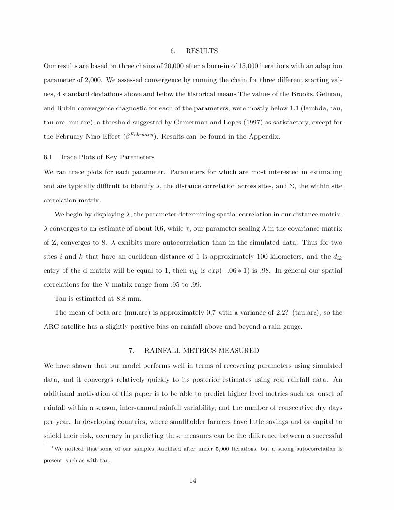
6. RESULTS
Our results are based on three chains of 20,000 after a burn-in of 15,000 iterations with an adaption
parameter of 2,000. We assessed convergence by running the chain for three different starting val-
ues, 4 standard deviations above and below the historical means.The values of the Brooks, Gelman,
and Rubin convergence diagnostic for each of the parameters, were mostly below 1.1 (lambda, tau,
tau.arc, mu.arc), a threshold suggested by Gamerman and Lopes (1997) as satisfactory, except for
the February Nino Effect (βFebruary). Results can be found in the Appendix.1
6.1 Trace Plots of Key Parameters
We ran trace plots for each parameter. Parameters for which are most interested in estimating
and are typically difficult to identify λ, the distance correlation across sites, and Σ, the within site
correlation matrix.
We begin by displaying λ, the parameter determining spatial correlation in our distance matrix.
λ converges to an estimate of about 0.6, while τ , our parameter scaling λ in the covariance matrix
of Z, converges to 8. λ exhibits more autocorrelation than in the simulated data. Thus for two
sites i and k that have an euclidean distance of 1 is approximately 100 kilometers, and the dik
entry of the d matrix will be equal to 1, then vik is exp(−.06 ∗ 1) is .98. In general our spatial
correlations for the V matrix range from .95 to .99.
Tau is estimated at 8.8 mm.
The mean of beta arc (mu.arc) is approximately 0.7 with a variance of 2.2? (tau.arc), so the
ARC satellite has a slightly positive bias on rainfall above and beyond a rain gauge.
7. RAINFALL METRICS MEASURED
We have shown that our model performs well in terms of recovering parameters using simulated
data, and it converges relatively quickly to its posterior estimates using real rainfall data. An
additional motivation of this paper is to be able to predict higher level metrics such as: onset of
rainfall within a season, inter-annual rainfall variability, and the number of consecutive dry days
per year. In developing countries, where smallholder farmers have little savings and or capital to
shield their risk, accuracy in predicting these measures can be the difference between a successful
1We noticed that some of our samples stabilized after under 5,000 iterations, but a strong autocorrelation is
present, such as with tau.
14

and devastating harvest. For example, yields can be heavily affected by planting a week too early
or too late with respect to rainfall onset. Knowing consecutive dry days helps in preparing for a
dry season, and inter-annual variability gives us a sense of the upper and lower bounds for rainfall
over time.
We begin by plotting first some basic posterior estimates for mean rainfall and the proportion
of wet days per month. We then follow with some of the harder to predict diagnostics: inter-annual
rainfall variability, probability of consecutive dry days, probability of rainfall onset.
8. DISCUSSION
We have considered a model where rainfall is a latent multivariate t-distribution, driven by seasonal
patterns, satellite measurement error, and within site correlation between time series. The model is
fitted using Monte Carlo methods with Gibbs and Metropolis Hastings sampling. Initial starting
values in the three chains are set at the historical means, and then four standard deviations
above and below the means. The model’s accuracy is tested on simulated data and performs well,
recovering all of our predetermined parameters. The hierarchical structure allows for fitting within
site correlations of various time series measured at a single location, as well across site spatial
correlations. Both features enable us to incorporate information on rainfall patterns that can
improve out of sample simulations of rainfall, as well as tougher to estimate rainfall characteristics:
inter-annual rainfall variability, probability of consecutive dry days, probability of rainfall onset.
The ability to incorporate spatial, temporal, and measurement correlations has important
policy implications. First, food insecurity is generally correlated over time and space in parallel
with rainfall patterns. Thus, predictions that incorporate these spatial patterns can allow for
better response to anticipated droughts and subsequent food shortages in a region. This is crucial
for aid organizations and first responders to such crises. Second, different satellite measurements
can detect and depict different weather patterns depending on their resolution and what they aim
to measure: cloud cover, vegetation, lights, etc. Incorporating multiple information sets around
a particular area can increase the accuracy with which we predict weather patterns by narrowing
the variance around the mean trends. Although this research does not present a new weather
generator for use by end-users, we hope that the methodological advances made will eventually
lead to such a tool.
15

9. APPENDIX
The full posterior can be written as
p(θθθ | YYY ) ∝S∏s=1
T∏t=1
Js∏j=1
p(Ystj |Wstj)p(Wstj | Zst, βARCs ,Σs, γst)p(Zst | βββZs , τ, λ)
p(βββZs |µµµ,σσσ)p(βARCs | µARC, τARC)
p(µµµ)p(σσσ)p(τ)p(λ)p(µARC)p(τARC)p(ΣΣΣs)p(γst),
where θθθ denotes the entire vector of parameters,
θθθ = {WWW,ZZZ,βββARC,ΣΣΣ, γγγ,βββZ , τ, λ,µµµ,σσσ, µARC, τARC}.
To sample from this posterior, we use MCMC. First we set initial values of λ, τ , µARC, τARC,
µp and σp (for p = 1, ..., 23), ΣΣΣs (for s = 1, ..., S), and γst (for s = 1, ..., S and p = 1, ..., P ). These
initial values are set to be overdispersed around rough estimates of the parameters based on fits
of smaller, simpler models to the data. Next we sample initial values of
βARCs | µARC, τARC (for s = 1, ..., S), (6)
βZsp | µp, σp (for s = 1, ..., 6 and p = 1, ..., P ), (7)
ZZZt | βββZ , λ, τ,XXXt (for t = 1, ..., N). (8)
Then, for iteration g = 1, 2, ...., G, where we set G = 5000, we perform the following steps:
1. Sample WWW | YYY ,γγγ,ZZZ,βββARC,ΣΣΣ.
The conditional posterior distribution of the length-Js latent rainfall vector for location s
and day t, WWW st, follows the multivariate normal distribution described in Equation 2 from
Section 3. Each element of this vector can be sampled, conditional on the other elements,
from a univariate normal distribution according to standard methods (cite). This draw is
made in one of three ways:
(a) Case 1: If Ystj > 0, then Wstj = Ystj ; in other words, no sample is drawn, but instead
the value of Wstj is fixed.
(b) Case 2: If Ystj = 0, then the univariate normal distribution from which Wstj is sampled
is truncated on the right by zero, since the model specifies that the latent rainfall
amount must be less than zero in this case.
16
(c) Case 3: If Ystj is missing, then the sample is drawn without any truncation, since the
missing observation, Ystj , could have been equal to zero or greater than zero.
2. Sample γγγ |WWW,ZZZ,βββARC,ΣΣΣ, α.
γst ∼ Γ(shape = (Js + α)/2, rate = 2/((WWW st −µµµWst )TΣ−1s (WWW st −µµµWst ) + α)),
where µµµWst = 1Zst +XXXARCs βARC
s , for s = (1, ..., S) and t = (1, ..., N), and α is set to 5.
3. Sample ZZZ |WWW,γγγ,βββARC,ΣΣΣ,βββZ , τ, λ.
The spatial mean rainfall vector can be sampled in closed form from a multivariate normal
distribution. To compute the mean and variance of its multivariate normal posterior distri-
bution, we “complete the square” twice. First, note that the posterior distribution of ZZZt is
proportional to
p(WWW | YYY ,γγγ,ZZZ,βββARC,ΣΣΣ)p(ZZZ | βββZ , τ, λ),
where both of these terms are multivariate normal probability distribution functions (PDFs).
In the first term, by treating ZZZ as unknown and the other parameters as known, one can see
that it is proportional to the multivariate normal PDF where
ZZZt ∼ NS(µµµZt ,ΣΣΣZt ),
where the sth element of the mean is given by
µZst = (1)TΣ−1s (WWW st −XXXARCs βARC
s )/(1TΣ−1s 1),
the variance of the sth element is given by
ΣZt[s] = 1/(γst1
TΣ−1s 1),
and the off-diagonal elements of ΣZt = 0.
Next, combining this term with the second term, which is also a multivariate normal PDF,
we compute the full conditional posterior distribution for ZZZt:
ZZZt ∼ NS
(((ΣΣΣZ
t )−1 + (σ2VVV )−1)−1(
(ΣΣΣZt )−1µµµZt + (σ2VVV )−1XXXtβββ
Z),(
(ΣΣΣZt )−1 + (σ2VVV )−1
)−1).
4. Sample βββARC |WWW,γγγ,ZZZ,ΣΣΣ, µARC, τARC from
βARCs ∼ N
(µWs /σ
2s(W ) + µARC/τ2ARC
1/σ2s(W ) + 1/τ2ARC
,1
1/σ2s(W ) + 1/τ2ARC
),
17

where
µWs =−(XXXARC
s )TΣΣΣ−1s∑N
t=1 γst(1Zst −WWW st)∑Tt=1 γst(XXX
ARCs )TΣ−1s XXXARC
s
and
σ2s(W ) = 1/N∑t=1
γst(XXXARCs )TΣ−1s XXXARC
s .
5. Sample ΣΣΣ |WWW,γγγ,ZZZ,βββARC from
Σs ∼ Inv-Wishart(
df = N + Js, , scale = diag(Js) +N∑t=1
γst(WWW st −µµµWst )(WWW st −µµµWst )T),
where µµµWst = 1Zst +XXXARCs βARC
s .
6. Sample βββZ | ZZZ, λ, τ,µµµ,σσσ.
βββZ is expressed as a 23×S matrix, but its posterior distribution will be drawn from a 23×S =
138-dimensional multivariate normal distribution. The variance, BBB, can be expressed as:
BBB =
((τ2VVV ⊗ (XXXTXXX)−1
)−1+(
Diag(S)⊗Diag(σσσ))−1)−1
,
where ⊗ is the Kronecker product. The conditional posterior mean of βββZ can be expressed
as:
βββZ
= BBB(
vec(XXXTZZZ(τ2VVV )−1) + (Diag(S) + Diag(σσσ))−1vec(µµµ1)),
where vec(AAA) indicates the stacked columns of the matrix AAA, and 1 denotes the 1 × 6 matrix
of ones, in this case.
7. Sample σσσ | βββZ ,µµµ.
We draw σp using a random-walk Metropolis step for p = 1, ..., P .
8. Sample µµµ | βββZ ,σσσ.
µp ∼ N(σ20β
Zp /(σ
2p/S + σ20), (1/σ20 + S/σ2p)
−1),
where σ0 = 5 as in equation [].
9. Sample λ | ZZZ,βββZ , τ .
We draw λ using a random-walk Metropolis step.
18

10. Sample τ | ZZZ,βββZ , λ, from
τ ∼ Inv-Gamma(a = 1 +NS/2, 1 + 1/2N∑t=1
(ZZZt −XXXtβββZ)TVVV −1(ZZZt −XXXtβββ
Z).
11. Sample µARC | βARC, τARC, from
µARC ∼ N
(SβARC/τ2ARC
1 + S/τ2ARC
,√
1 + S/τ2ARC
)
12. Sample τARC | βARC, µARC.
We draw τARC using a random-walk Metropolis step.
REFERENCES
Apipattanavis, S., Podesta, G., Rajagopalan, B., and Katz, R. W. (2007), “A semiparametric
multivariate and multisite weather generator,” Water Resources Research, 43(11), 19.
Baigorria, G. a., and Jones, J. W. (2010), “GiST: A Stochastic Model for Generating Spatially
and Temporally Correlated Daily Rainfall Data,” Journal of Climate, 23(22), 5990–6008.
URL: http://journals.ametsoc.org/doi/abs/10.1175/2010JCLI3537.1
Bell, A. R., Osgood, D. E., Cook, B. I., Anchukaitis, K. J., McCarney, G. R., Greene, A. M.,
Buckley, B. M., and Cook, E. R. (2013), “Paleoclimate histories improve access and sustainabil-
ity in index insurance programs,” Global Environmental Change, 23(4), 774–781.
URL: http://linkinghub.elsevier.com/retrieve/pii/S0959378013000502
Buishand, T. A. (1978), “Some remarks on the use of daily rainfall models,” Journal of Hydrology,
36, 295–308.
Carey-Smith, T., Sansom, J., and Thomson, P. (2014), “A hidden seasonal switching model for
multisite daily rainfall,” Water Resources Research, 50(1), 257–272.
URL: http://doi.wiley.com/10.1002/2013WR014325
Coe, R., and Stern, R. D. (1984), “Royal Statistical Society Analysis of Daily Rainfall Data,”
Journal of the Royal Statistical Society. Series A (General), 147(1).
19

Dastidar, A. G., Ghosh, D., Dasgupta, S., and De, U. K. (2010), “Higher order Markov chain
models for monsoon rainfall over West Bengal, India,” Indian Journal of Radio AND Space
Physics, 39(February), 39–44.
Fasso, A., and Finazzi, F. (2011), “Maximum likelihood estimation of the dynamic coregionaliza-
tion model with heterotopic data,” Environmetrics, 22(6), 735–748.
URL: http://doi.wiley.com/10.1002/env.1123
Furrer, E. M., and Katz, R. W. (2008), “Improving the simulation of extreme precipitation events
by stochastic weather generators,” Water Resources Research, 44(12), 1–13.
Gabriel, K. R., and Neumann, J. (1962), “A Markov chain model for daily rainfall occurrence at
Tel Aviv,” Quarterly Journal of the Royal Meteorological Society, 88(375), 90–95.
URL: http://dx.doi.org/10.1002/qj.49708837511\nhttp://onlinelibrary.wiley.com/doi/10.1002/qj.49708837511/abstract
Gamerman, D., and Lopes, H. F. (1997), Markov Chain Monte Carlo, Stochastic Simulation for
Bayesian Inference., London: Chapman and Hall.
Ghile, Y., and Schulze, R. (2009), “Use of an Ensemble Re-ordering Method for disaggregation of
seasonal categorical rainfall forecasts into conditioned ensembles of daily rainfall for hydrological
forecasting,” Journal of Hydrology, 371(1-4), 85–97.
URL: http://linkinghub.elsevier.com/retrieve/pii/S0022169409001759
Giannini, A., Hansen, J., Holthaus, E., Ines, A., Kaheil, Y., Karnauskas, K., Mclaurin, M., Osgood,
D., Robertson, A., Shirley, K., and Vicarelli, M. (2009), “Desigingin Index Based Weather
Insurance for Farmers in Central America,” IRI Technical Report 09-01, (March).
Greatrex, H. (2012), “The application of seasonal rainfall forecasts and satellite rainfall estimates
to seasonal crop yield forecasting for Africa,” , (May), 320.
Greatrex, H., Hansen, J., Garvin, S., Diro, R., Blakeley, S., Guen, M. L., Rao, K., and Osgood,
D. (2015), “Scaling up index insurance for smallholder farmers : Recent evidence and insights,”
CCAFS Report, (No.14), 1–32.
Hauser, T., and Demirov, E. (2013), “Development of a stochastic weather generator for the sub-
polar North Atlantic,” Stochastic Environmental Research and Risk Assessment, 27(7), 1533–
20
1551.
URL: http://link.springer.com/10.1007/s00477-013-0688-z
Jones, P. G., and Thornton, P. K. (1993), “A rainfall generator for agricultural applications in the
tropics,” Agricultural and Forest Meteorology, 63(1-2), 1–19.
URL: http://www.sciencedirect.com/science/article/pii/016819239390019E
Katz, R. W. (1977), “Precipitation as a Chain-Dependent Process,”.
URL: http://dx.doi.org/10.1175/1520-0450(1977)016¡0671:PAACDP¿2.0.CO\n2
Kleiber, W., Katz, R. W., and Rajagopalan, B. (2012), “Daily spatiotemporal precipitation sim-
ulation using latent and transformed Gaussian processes,” Water Resources Research, 48(Jan-
uary), 1–18.
Lall, U., and Sharma, A. (1996), “A nearest neighbor bootstrap for resampling hydrologic time
series,” Water Resources Research, 32(3), 679–693.
Lennartsson, J., Baxevani, A., and Chen, D. (2008), “Modelling precipitation in Sweden using
multiple step markov chains and a composite model,” Journal of Hydrology, 363(1-4), 42–59.
URL: http://linkinghub.elsevier.com/retrieve/pii/S0022169408004848
Lima, C. H., Lall, U., Troy, T. J., and Devineni, N. (2015), “A climate informed model for
nonstationary flood risk prediction: Application to Negro River at Manaus, Amazonia,” Journal
of Hydrology, 522, 594–602.
URL: http://linkinghub.elsevier.com/retrieve/pii/S0022169415000153
Osgood, D., and Shirley, K. E. (2012), “The Value of Information in Index Insurance for Farmers
in Africa,” in The Value of Information, eds. R. Laxminarayan, and M. K. Macauley, Dordrecht:
Springer Netherlands, pp. 1–18.
URL: http://link.springer.com/10.1007/978-94-007-4839-2
Racsko, P., Szeidl, L., and Semenov, M. (1991), “A serial approach to local stochastic weather
models,” Ecological Modelling, 57, 27–41.
Rajagopalan, B., and Lall, U. (1999), “A k-nearest-neighbor simulator for daily precipitation and
21

other weather variables,” Water resources research, 35(10), 3089–3101.
URL: http://onlinelibrary.wiley.com/doi/10.1029/1999WR900028/full
Richardson, C. W. C. (1981), “Stochastic simulation of daily precipitation, temperature, and solar
radiation,” Water Resources Research, 17(1), 182.
URL: http://onlinelibrary.wiley.com/doi/10.1029/WR017i001p00182/full
Sans, B., and Guenni, L. (2015), “Royal Statistical Society Venezuelan rainfall data analysed by
using a Bayesian space-time model,” , 48(3).
Sanso, B., and Guenni, L. (2000), “A Nonstationary Multisite Model for Rainfall,” Journal of the
American Statistical Association, 95(452), 1089–1100.
URL: http://www.tandfonline.com/doi/abs/10.1080/01621459.2000.10474305
Semenov, M. a. (2008), “Simulation of extreme weather events by a stochastic weather generator,”
Climate Research, 35(3), 203–212.
Srivastav, R. K., and Simonovic, S. P. (2015), “Multi-site, multivariate weather generator using
maximum entropy bootstrap,” Climate Dynamics, 44(11-12), 3431–3448.
URL: http://link.springer.com/10.1007/s00382-014-2157-x
Thom, H. C. S. (1958), “a Note on the Gamma Distribution,” Monthly Weather Review, 86(3), 117–
122.
Verdin, A., Rajagopalan, B., Kleiber, W., and Katz, R. W. (2015), “Coupled stochastic weather
generation using spatial and generalized linear models,” Stochastic Environmental Research and
Risk Assessment, 29(2), 347–356.
URL: http://link.springer.com/10.1007/s00477-014-0911-6
Wilks, D. (1992), “Adapting Stochastic Weather Generation Algorithms for Cimate Chnage Stud-
ies,” Climatic Change, 22, 67–84.
Wilks, D. (1998), “Multisite generalization of a daily stochastic precipitation generation model,”
Journal of Hydrology, 210(1-4), 178–191.
URL: http://www.sciencedirect.com/science/article/pii/S0022169498001863
22

Wilks, D. S. (1989), “Rainfall Intensity, the Weibull Distribution, and Estimation of Daily Surface
Runoff,”.
Wilks, D. S., and Wilby, R. L. (1999), “The weather generation game: a review of stochastic
weather models,” Progress in Physical Geography, 23(3), 329–357.
URL: http://ppg.sagepub.com/cgi/doi/10.1177/030913339902300302
Young, K. C. (1994), “A Multivariate Chain Model for Simulating Climatic Parameters from Daily
Data,”.
23