hierarchical models in the brain · 2011-03-09 · hierarchical models in the brain karl friston*...

Hierarchical Models in the BrainKarl Friston*

The Wellcome Trust Centre of Neuroimaging, University College London, London, United Kingdom

Abstract

This paper describes a general model that subsumes many parametric models for continuous data. The model compriseshidden layers of state-space or dynamic causal models, arranged so that the output of one provides input to another. Theensuing hierarchy furnishes a model for many types of data, of arbitrary complexity. Special cases range from the generallinear model for static data to generalised convolution models, with system noise, for nonlinear time-series analysis.Crucially, all of these models can be inverted using exactly the same scheme, namely, dynamic expectation maximization.This means that a single model and optimisation scheme can be used to invert a wide range of models. We present themodel and a brief review of its inversion to disclose the relationships among, apparently, diverse generative models ofempirical data. We then show that this inversion can be formulated as a simple neural network and may provide a usefulmetaphor for inference and learning in the brain.

Citation: Friston K (2008) Hierarchical Models in the Brain. PLoS Comput Biol 4(11): e1000211. doi:10.1371/journal.pcbi.1000211

Editor: Olaf Sporns, Indiana University, United States of America

Received June 30, 2008; Accepted September 19, 2008; Published November 7, 2008

Copyright: � 2008 Karl Friston. This is an open-access article distributed under the terms of the Creative Commons Attribution License, which permitsunrestricted use, distribution, and reproduction in any medium, provided the original author and source are credited.

Funding: This work was supported by the Wellcome Trust.

Competing Interests: The author has declared that no competing interests exist.

* E-mail: [email protected]

Introduction

This paper describes hierarchical dynamic models (HDMs) and

reviews a generic variational scheme for their inversion. We then

show that the brain has evolved the necessary anatomical and

physiological equipment to implement this inversion, given sensory

data. These models are general in the sense that they subsume

simpler variants, such as those used in independent component

analysis, through to generalised nonlinear convolution models.

The generality of HDMs renders the inversion scheme a useful

framework that covers procedures ranging from variance compo-

nent estimation, in classical linear observation models, to blind

deconvolution, using exactly the same formalism and operational

equations. Critically, the nature of the inversion lends itself to a

relatively simple neural network implementation that shares many

formal similarities with real cortical hierarchies in the brain.

Recently, we introduced a variational scheme for model inversion

(i.e., inference on models and their parameters given data) that

considers hidden states in generalised coordinates of motion. This

enabled us to derive estimation procedures that go beyond

conventional approaches to time-series analysis, like Kalman or

particle filtering. We have described two versions; variational

filtering [1] and dynamic expectation maximisation (DEM; [2])

that use free and fixed-form approximations to the posterior or

conditional density respectively. In these papers, we used hierarchi-

cal dynamic models to illustrate how the schemes worked in practice.

In this paper, we focus on the model per se and the relationships

among its special cases. We will use DEM to show how their

inversion relates to conventional treatments of these special cases.

A key aspect of DEM is that it was developed with neuronal

implementation in mind. This constraint can be viewed as

formulating a neuronally inspired estimation and inference

framework or conversely, as providing heuristics that may inform

our understanding of neuronal processing. The basic ideas have

already been described, in the context of static models, in a series

of papers [3–5] that entertain the notion that the brain may use

empirical Bayes for inference about its sensory input, given the

hierarchical organisation of cortical systems. In this paper, we

generalise this idea to cover hierarchical dynamical systems and

consider how neural networks could be configured to invert

HDMs and deconvolve sensory causes from sensory input.

This paper comprises five sections. In the first, we introduce

hierarchical dynamic models. These cover many observation or

generative models encountered in the estimation and inference

literature. An important aspect of these models is their formulation

in generalised coordinates of motion; this lends them a hierarchal

form in both structure and dynamics. These hierarchies induce

empirical priors that provide structural and dynamic constraints,

which can be exploited during inversion. In the second and third

sections, we consider model inversion in general terms and then

specifically, using dynamic expectation maximisation (DEM). This

reprises the material in Friston et al. [2] with a special focus on

HDMs. DEM is effectively a variational or ensemble learning

scheme that optimises the conditional density on model states (D-

step), parameters (E-step) and hyperparameters (M-step). It can

also be regarded as a generalisation of expectation maximisation

(EM), which entails the introduction of a deconvolution or D-step

to estimate time-dependent states. In the fourth section, we review

a series of HDMs that correspond to established models used for

estimation, system identification and learning. Their inversion is

illustrated with worked-examples using DEM. In the final section,

we revisit the DEM steps and show how they can be formulated as

a simple gradient ascent using neural networks and consider how

evoked brain responses might be understood in terms of inference

under hierarchical dynamic models of sensory input.

NotationTo simplify notation we will use fx := fx(x) = hxf = hf/hx to denote

the partial derivative of the function, f, with respect to the variable

x. We also use x = htx for temporal derivatives. Furthermore, we

PLoS Computational Biology | www.ploscompbiol.org 1 November 2008 | Volume 4 | Issue 11 | e1000211

will be dealing with variables in generalised coordinates of motion,

which will be denoted by a tilde; x := [x,x9,x0,…]T = [x[0],x[1],x[2],…]T,

where x[i] denotes ith order motion. A point in generalised

coordinates can be regarded as encoding the instantaneous trajectory

of a variable, in the sense it prescribes its location, velocity,

acceleration etc.

Materials and Methods

Hierarchical Dynamic ModelsIn this section, we cover hierarchal models for dynamic systems.

We start with the basic model and how generalised motion

furnishes empirical priors on the dynamics of the model’s hidden

states. We then consider hierarchical forms and see how these

induce empirical priors in a structural sense. We will try to relate

these perspectives to established treatments of empirical priors in

static and state-space models.

Hierarchical dynamic causal models. Dynamic causal

models are probabilistic generative models p(y,W) based on state-

space models. As such, they entail the likelihood, p(y|W) of getting

some data, y, given some parameters W= {x,v,h,l} and priors on

those parameters, p(W). We will see that the parameters subsume

different quantities, some of which change with time and some which

do not. These models are causal in a control-theory sense because

they are state-space models, formulated in continuous time.

State-pace models in generalised coordinates. A

dynamic input-state-output model can be written as

y~g x,vð Þzz

_xx~f x,vð Þzwð1Þ

The continuous nonlinear functions f and g of the states are

parameterised by h. The states v(t) can be deterministic, stochastic,

or both. They are variously referred to as inputs, sources or causes.

The states x(t) meditate the influence of the input on the output

and endow the system with memory. They are often referred to as

hidden states because they are seldom observed directly. We

assume the stochastic terms (i.e., observation noise) z(t) are

analytic, such that the covariance of z = [z,z9,z0,…]T is well

defined; similarly for the system or state noise, w(t), which

represents random fluctuations on the motion of the hidden states.

Under local linearity assumptions (i.e., ignoring high-order

derivatives of the generative model functions), the generalised

output or response y = [y,y9,y0,…]T obtains from recursive

differentiation with respect to time using the chain rule

y~g x,vð Þzz

y’~gxx’zgvv’zz’

y’’~gxx’’zgvv’’zz’’

..

.

_xx~x’~f x,vð Þzw

_xx’~x’’~fxx’zfvv’zw’

_xx’’~x’’’~fxx’’zfvv’’zw’’

..

.

ð2Þ

Note that the derivatives are evaluated at each point in time and

the linear approximation is local to the current state. The first

(observer) equation show that the generalised states u = [v,x,]T are

needed to generate a generalised response that encodes a path or

trajectory. The second (state) equations enforce a coupling

between neighbouring orders of motion of the hidden states and

confer memory on the system.

At this point, readers familiar with standard state-space models

may be wondering where all the extra equations in Equation 2

come from and, in particular, what the generalised motions; w9,

w0, … represent. These terms always exist but are ignored in

standard treatments based on the theory of Markovian processes

[6]. This is because standard Markovian (c.f., Wiener) processes

have generalised motion that has infinite variance and are

infinitely ‘jagged’ or rough. This means w9, w0, … and x0, x-, …

have no precision (inverse variance) and can be ignored with

impunity. It is important to realise that this approximation is not

appropriate for real or actual fluctuations, as noted at the

inception of the standard theory; ‘‘a certain care must be taken

in replacing an actual process by Markov process, since Markov

processes have many special features, and, in particular, differ

from the processes encountered in radio engineering by their lack

of smoothness… any random process actually encountered in

radio engineering is analytic, and all its derivative are finite with

probability one’’ ([6], pp 122–124). So why have standard state-

space models, and their attending inversion schemes like Kalman

filtering, dominated the literature over the past half-century?

Partly because it is convenient to ignore generalised motion and

partly because they furnish reasonable approximations to

fluctuations over time-scales that exceed the correlation time of

the random processes: ‘‘Thus the results obtained by applying the

techniques of Markov process theory are valuable only to the

extent to which they characterise just these ‘large-scale’ fluctua-

tions’’ ([6], p 123). However, standard models fail at short time-

scales. This is especially relevant in this paper because the brain

has to model continuous sensory signals on a fast time-scale.

Having said this, it is possible to convert the generalised state-

space model in Equation 2 into a standard form by expressing the

components of generalised motion in terms of a standard

[uncorrelated] Markovian process, z(t):

wzc1w0zc2w00z . . . zcnw n½ �~z[

_xx~x0

_xx0~x00

..

.

cn _xx n½ �~f x,vð ÞzXn

i~1

cifx{ci{1ð Þx i½ �zcifvv i½ ��

zz

ð3Þ

Author Summary

Models are essential to make sense of scientific data, but theymay also play a central role in how we assimilate sensoryinformation. In this paper, we introduce a general model thatgenerates or predicts diverse sorts of data. As such, itsubsumes many common models used in data analysis andstatistical testing. We show that this model can be fitted todata using a single and generic procedure, which means wecan place a large array of data analysis procedures within thesame unifying framework. Critically, we then show that thebrain has, in principle, the machinery to implement thisscheme. This suggests that the brain has the capacity toanalyse sensory input using the most sophisticated algo-rithms currently employed by scientists and possibly modelsthat are even more elaborate. The implications of this workare that we can understand the structure and function of thebrain as an inference machine. Furthermore, we can ascribevarious aspects of brain anatomy and physiology to specificcomputational quantities, which may help understand bothnormal brain function and how aberrant inferences resultfrom pathological processes associated with psychiatricdisorders.

Hierarchical Models


The first line encodes the autocorrelation function or spectral

density of the fluctuations w(t) in term of smoothness

parameters, c1,…cn, where n is the order of generalised motion.

These parameters can be regarded as the coefficients of a

polynomial expansion Pn(ht)w = z(t) (see [6], Equation 4.288 and

below). The second line obtains by substituting Equation 2 into

the first and prescribes a standard state-space model, whose

states cover generalised motion; x[0],…,x[n]. When n = 0 we

recover the state equation in Equation 1, namely, x = f(x,v)+z.

This corresponds to the standard Markovian approximation

because the random fluctuations are uncorrelated and w = z;

from Equation 3. When n = 1)w+c1w9 = z, the fluctuations w(t)

correspond to an exponentially correlated process, with a decay

time of c1 ([6], p 121). However, generally n = ‘: ‘‘Therefore we

cannot describe an actual process within the framework of

Markov process theory, and the more accurately we wish to

approximate such a process by a Markov process, the more

components the latter must have.’’ ([6], p 165). See also [7]

(pp 122–125) for a related treatment.

If there is a formal equivalence between standard and

generalised state-space models, why not use the standard

formulation, with a suitably high-order approximation? The

answer is that we do not need to; by retaining an explicit

formulation in generalised coordinates we can devise a simple

inversion scheme (Equation 23) that outperforms standard

Markovian techniques like Kalman filtering. This simplicity is

important because we want to understand how the brain inverts

dynamic models. This requires a relatively simple neuronal

implementation that could have emerged through natural

selection. From now on, we will reserve ‘state-space models’

(SSM) for standard n = 0 models that discount generalised

motion and, implicitly, serial correlations among the random

terms. This means we can treat SSMs as special cases of

generalised state-space models, in which the precision of

generalised motion on the states noise is zero.

Probabilistic dynamic models. Given the form of

generalised state-space models we now consider what they entail

as probabilistic models of observed signals. We can write

Equation 2 compactly as

~yy~~ggz~zz

D~xx~~ff z~wwð4Þ

Where the predicted response g = [g,g9,g0,…]T and motion

f = [f,f 9,f 0,…]T in the absence of random fluctuations are

g~g x,vð Þ

g’~gxx’zgvv’

g’’~gxx’’zgvv’’

..

.

f ~f x,vð Þ

f ’~fxx’zfvv’

f ’’~fxx’’zfvv’’

..

.

and D is a block-matrix derivative operator, whose first

leading-diagonal contains identity matrices. This operator simply

shifts the vectors of generalised motion so x[i] that is replaced by

x[i+1].

Gaussian assumptions about the fluctuations p ~z� �

~N ~zz : 0,~SSz� �

provide the likelihood, p(y|x,v). Similarly, Gaussian assumptions

about state-noise p ~wwð Þ~N ~ww : 0,~SSw� �

furnish empirical priors,

p(x|v) in terms of predicted motion

p ~yy,~xx,~vvð Þ~p ~yy ~xx,~vvjð Þp ~xx,~vvð Þ

p ~yy ~xx,~vvjð Þ~N ~yy : ~gg,~SSz� �

p ~xx,~vvð Þ~p ~xx ~vvjð Þp ~vvð Þ

p ~xx ~vvjð Þ~N D~xx : ~ff ,~SSw� � ð5Þ

We will assume Gaussian priors p ~vvð Þ~N ~vv : ~gg,~SSv� �

on the

generalised causes, with mean ~gg : ~~ggv and covariance ~SSv. The

density on the hidden states p(x|v) is part of the prior on quantities

needed to evaluate the likelihood of the response or output. This

prior means that low-order motion constrains high-order motion

(and vice versa). These constraints are discounted in standard state-

space models because the precision on the generalised motion of a

standard Markovian process is zero. This means the only constraint

is mediated by the prior p(x|x,v). However, it is clear from Equation 5

that high-order terms contribute. In this work, we exploit these

constraints by adopting more plausible models of noise, which are

encodedbytheircovariances ~SS lð Þz and ~SS lð Þw (orprecisions ~PP lð Þz and~PP lð Þw). These are functions of unknown hyperparameters, l which

control the amplitude and smoothness of the random fluctuations.

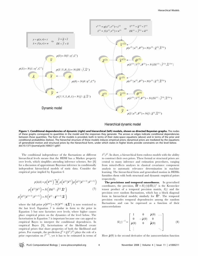
Figure 1 (left) shows the directed graph depicting the conditional

dependencies implied by this model. Next, we consider hierarchal

models that provide another form of hierarchical constraint. It is useful

to note that hierarchical models are special cases of Equation 1, in the

sense that they are formed by introducing conditional independencies

(i.e., removing edges in Bayesian dependency graphs).

Hierarchical forms. HDMs have the following form, which

generalises the (m = 1) model above

y~g x 1ð Þ,v 1ð Þ� �

zz 1ð Þ

_xx 1ð Þ~f x 1ð Þ,v 1ð Þ� �

zw 1ð Þ

..

.

v i{1ð Þ~g x ið Þ,v ið Þ� �

zz ið Þ

_xx ið Þ~f x ið Þ,v ið Þ� �

zw ið Þ

..

.

v mð Þ~gzz mz1ð Þ

ð6Þ

Again, f (i) := f(x(i),v(i)) and g(i) := g(x(i),v(i)) are continuous nonlinear

functions of the states. The processes z(i) and w(i) are conditionally

independent fluctuations that enter each level of the hierarchy.

These play the role of observation error or noise at the first level

and induce random fluctuations in the states at higher levels. The

causes v = [v(1),…,v(m)]T link levels, whereas the hidden states

x = [x(1),…,x(m)]T link dynamics over time. The corresponding

directed graphical model is shown in Figure 1 (right). In

hierarchical form, the output of one level acts as an input to the

next. When the state-equations are linear, the hierarchy performs

successive convolutions of the highest level input, with random

fluctuations entering at each level. However, inputs from higher

levels can also enter nonlinearly into the state equations and can

be regarded as changing its control parameters to produce quite

complicated generalised convolutions with ‘deep’ (i.e.,

hierarchical) structure.

Hierarchical Models


The conditional independence of the fluctuations at different

hierarchical levels means that the HDM has a Markov property

over levels, which simplifies attending inference schemes. See [8]

for a discussion of approximate Bayesian inference in conditionally

independent hierarchical models of static data. Consider the

empirical prior implied by Equation 6

p ~xx,~vvð Þ~p ~vv mð Þ� �

Pm{1

i~1p ~xx ið Þ ~vv ið Þ��

p ~vv ið Þ ~xx iz1ð Þ,~vv iz1ð Þ�� p ~xx ið Þ ~vv ið Þ��

~N D~xx ið Þ : ~ff ið Þ,~SSw� �

p ~vv ið Þ ~xx iz1ð Þ,~vv iz1ð Þ�� ~N ~vv ið Þ : ~gg iz1ð Þ,~SSz

� � ð7Þ

where the full prior p ~vv mð Þ� �~N ~vv mð Þ : ~gg,~SSv

� �is now restricted to

the last level. Equation 7 is similar in form to the prior in

Equation 5 but now factorises over levels; where higher causes

place empirical priors on the dynamics of the level below. The

factorisation in Equation 7 is important because one can appeal to

empirical Bayes to interpret the conditional dependences. In

empirical Bayes [9], factorisations of the likelihood create

empirical priors that share properties of both the likelihood and

priors. For example, the prediction g(i) = g(x(i),v(i)) plays the role of a

prior expectation on v(i21), yet it has to be estimated in terms of

x(i),v(i). In short, a hierarchical form endows models with the ability

to construct their own priors. These formal or structural priors are

central to many inference and estimation procedures, ranging

from mixed-effects analyses in classical covariance component

analysis to automatic relevance determination in machine

learning. The hierarchical form and generalised motion in HDMs

furnishes them with both structural and dynamic empirical priors

respectively.

The precisions and temporal smoothness. In generalised

coordinates, the precision, ~PPz~S cð Þ6P lð Þz is the Kronecker

tensor product of a temporal precision matrix, S(c) and the

precision over random fluctuations, which has a block diagonal

form in hierarchical models; similarly for ~PPw. The temporal

precision encodes temporal dependencies among the random

fluctuations and can be expressed as a function of their

autocorrelations

S cð Þ{1~

1 0 €rr 0ð Þ . . .

0 {€rr 0ð Þ 0

€rr 0ð Þ 0 €€rr€rr 0ð Þ...

P

266664377775 ð8Þ

Here €rr 0ð Þ is the second derivative of the autocorrelation function

Figure 1. Conditional dependencies of dynamic (right) and hierarchical (left) models, shown as directed Bayesian graphs. The nodesof these graphs correspond to quantities in the model and the responses they generate. The arrows or edges indicate conditional dependenciesbetween these quantities. The form of the models is provided, both in terms of their state-space equations (above) and in terms of the prior andconditional probabilities (below). The hierarchal structure of these models induces empirical priors; dynamical priors are mediated by the equationsof generalised motion and structural priors by the hierarchical form, under which states in higher levels provide constraints on the level below.doi:10.1371/journal.pcbi.1000211.g001

Hierarchical Models


evaluated at zero. This is a ubiquitous measure of roughness in the

theory of stochastic processes [10]. Note that when the random

fluctuations are uncorrelated, the curvature (and higher

derivatives) of the autocorrelation are infinite. In this instance,

the precision of high-order motion falls to zero. This is the limiting

case assumed by state-space models; it corresponds to the

assumption that incremental fluctuations are independent (c.f., a

Wiener process or random walk). Although, this is a convenient

assumption that is exploited in conventional Bayesian filtering

schemes and appropriate for physical systems with Brownian

processes, it is less plausible for biological and other systems, where

random fluctuations are themselves generated by dynamical

systems ([6], p 81).

S(c) can be evaluated for any analytic autocorrelation function.

For convenience, we assume that the temporal correlations have

the same Gaussian form. This gives

S cð Þ{1~

1 0 { 12

c . . .

0 12

c 0

{ 12

c 0 34

c2

..

.P

2666664

3777775 ð9Þ

Here, c is the precision parameter of a Gaussian autocorrelation

function. Typically, c.1, which ensures the precisions of high-

order motion converge quickly. This is important because it

enables us to truncate the representation of an infinite number of

generalised coordinates to a relatively small number; because high-

order prediction errors have a vanishingly small precision. An

order of n = 6 is sufficient in most cases [1]. A typical example is

shown in Figure 2, in generalised coordinates and after projection

onto the time-bins (using a Taylor expansion, whose coefficients

comprise the matrix E). It can be seen that the precision falls

quickly with order and, in this case, we can consider just six orders

of motion, with no loss of precision.

When dealing with discrete time-series it is necessary to map the

trajectory implicit in the generalised motion of the response onto

discrete samples, [y(t1),…,y(tN)]T = Ey(t) (note that this is not

necessary with continuous data such as sensory data sampled by

the brain). After this projection, the precision falls quickly over

time-bins (Figure 2, right). This means samples in the remote past

or future do not contribute to the likelihood and the inversion of

discrete time-series data can proceed using local samples around

the current time bin; i.e., it can operate ‘on-line’.

Energy functions. We can now write down the exact form of

the generative model. For dynamic models, under Gaussian

assumptions about the random terms, we have a simple quadratic

form (ignoring constants)

ln p ~yy,~xx,~vv h,ljð Þ~ 1

2ln ~PP�� { 1

2~eeT ~PP~ee

~PP~~PPz

~PPw

" #

~ee~~eev~~yy{~gg

~eex~D~xx{~ff

" # ð10Þ

The auxiliary variables ~ee tð Þ comprise prediction errors for the

generalised response and motion of hidden states, where g(t) and f(t)

are the respective predictions, whose precision is encoded by ~PP lð Þ.The use of prediction errors simplifies exposition and may be used

in neurobiological implementations (i.e., encoded explicitly in the

brain; see last section and [4]). For hierarchical models, the

prediction error on the response is supplemented with prediction

errors on the causes

ev~

y

v 1ð Þ

..

.

v mð Þ

266664377775{

g 1ð Þ

g 2ð Þ

..

.

g

266664377775 ð11Þ

Note that the data and priors enter the prediction error at the

lowest and highest level respectively. At intermediate levels the

prediction errors, v(i21)2g(i) mediate empirical priors on the causes.

In the next section, we will use a variational inversion of the

HDM, which entails message passing between hierarchical levels.

These messages are the prediction errors and their influence rests

on the derivatives of the prediction error with respect to the

unknown states

~eeu~~eev

v ~eevx

~eexv ~eex

x

� �~{

I6 gv{DTð Þ I6gx

I6fv I6fxð Þ{D

� �ð12Þ

This form highlights the role of causes in linking successive

hierarchical levels (the DT matrix) and the role of hidden states

in linking successive temporal derivatives (the D matrix). The DT

in the upper-left block reflects the fact that that the prediction

error on the causes depends on causes at that level and the lower

level being predicted; e(i)v = v(i21)2g(x(i),v(i)). The D in the lower-

right block plays a homologous role, in that the prediction error

on the motion of hidden states depends on motion at that order

and the higher order; e[i]x = x[i+1]2f(x[i],v[i]).

These constraints on the structural and dynamic form of the

system are specified by the functions g = [g(1),…,g(m)]T and

f = [f(1),…,f(m)]T, respectively. The partial derivatives of these

functions have a block diagonal form, reflecting the model’s

hierarchical separability

Figure 2. Image representations of the precision matricesencoding temporal dependencies among the generalisedmotion of random fluctuations. The precision in generalisedcoordinates (left) and over discrete samples in time (right) are shownfor a roughness of c = 4 and seventeen observations (with an orderof n = 16). This corresponds to an autocorrelation function whose widthis half a time bin. With this degree of temporal correlation only a few(i.e., five or six) discrete local observations are specified with anyprecision.doi:10.1371/journal.pcbi.1000211.g002

Hierarchical Models


gv~

g1ð Þ

v

0 P

P gmð Þ

v

0

2666664

3777775 gx~

g1ð Þ

x

0 P

P gmð Þ

x

0

2666664

3777775

fv~

f1ð Þ

v

P

fmð Þ

v

26643775 fx~

f1ð Þ

x

P

fmð Þ

x

26643775

ð13Þ

Note that the partial derivatives of g(x,v) have an extra row to

accommodate the top level. To complete model specification we

need priors on the parameters and hyperparameters. We will

assume these are Gaussian, where (ignoring constants)

ln p hð Þ~ 1

2ln Ph�� { 1

2ehTPheh

ln p lð Þ~ 1

2ln Pl�� { 1

2elTPlel

eh~h{gh

el~l{gl

ð14Þ

Summary. In this section, we have introduced hierarchical

dynamic models in generalised coordinates of motion. These

models are about as complicated as one could imagine; they

comprise causes and hidden states, whose dynamics can be

coupled with arbitrary (analytic) nonlinear functions.

Furthermore, these states can have random fluctuations with

unknown amplitude and arbitrary (analytic) autocorrelation

functions. A key aspect of the model is its hierarchical form,

which induces empirical priors on the causes. These recapitulate

the constraints on hidden states, furnished by the hierarchy

implicit in generalised motion. We now consider how these

models are inverted.

Model InversionThis section considers variational inversion of models under

mean-field and Laplace approximations, with a special focus on

HDMs. This treatment provides a heuristic summary of the

material in [2]. Variational Bayes is a generic approach to model

inversion that approximates the conditional density p(W|y,m) on

some model parameters, W, given a model m and data y. This is

achieved by optimising the sufficient statistics (e.g., mean and

variance) of an approximate conditional density q(W)with respect to

a lower bound on the evidence (marginal or integrated likelihood)

p(y|m) of the model itself. These two quantities are used for

inference on the parameters of any given model and on the model

per se. [11–15]. The log-evidence for any parametric model can be

expressed in terms of a free-energy F(y,q) and a divergence term,

for any density q(W) on the unknown quantities

ln p ~yy mjð Þ~FzD q qð Þ p q ~yy,mjð Þkð Þ[

F~Sln p ~yy,qð ÞTq{Sln q qð ÞTq

ð15Þ

The free-energy comprises the internal energy, U(y,W) = ln p(y,W)

expected under q(W) and an entropy term, which is a measure of its

uncertainty. In this paper, energies are the negative of the

corresponding quantities in physics; this ensures the free-energy

increases with log-evidence. Equation 15 indicates that F(y,q) is a

lower-bound on the log-evidence because the cross-entropy or

divergence term is always positive.

The objective is to optimise q(W) by maximising the free-energy

and then use F<ln p(y|m) as a lower-bound approximation to the

log-evidence for model comparison or averaging. Maximising the

free-energy minimises the divergence, rendering q(W)<p(W|y,m) an

approximate posterior, which is exact for simple (e.g., linear)

systems. This can then be used for inference on the parameters of

the model selected.

Invoking an arbitrary density, q(W) converts a difficult integra-

tion problem (inherent in computing the evidence; see discussion)

into an easier optimisation problem. This rests on inducing a

bound that can be optimised with respect to q(W). To finesse

optimisation, one usually assumes q(W) factorises over a partition of

the parameters

q qð Þ~Pi

q qi� �

q~ u,h,lf gð16Þ

In statistical physics this is called a mean-field approximation. This

factorisation means that one assumes the dependencies between

different sorts of parameters can be ignored. It is a ubiquitous

assumption in statistics and machine learning. Perhaps the most

common example is a partition into parameters coupling causes to

responses and hyperparameters controlling the amplitude or

variance of random effects. This partition greatly simplifies the

calculation of things like t-tests and implies that, having seen some

data, knowing their variance does not tell you anything more

about their mean. Under our hierarchical dynamic model we will

appeal to separation of temporal scales and assume,

q(W) = q(u(t))q(h)q(l), where u = [v,x,]T are generalised states. This

means that, in addition to the partition into parameters and

hyperparameters, we assume conditional independence between

quantities that change (states) and quantities that do not

(parameters and hyperparameters).

In this dynamic setting q(u(t)) and the free-energy become

functionals of time. By analogy with Lagrangian mechanics, this

calls on the notion of action. Action is the anti-derivative or path-

integral of energy. We will denote the action associated with the

free energy by F, such that htF = F. We now seek q(Wi) that

maximise the action. It is fairly easy to show [2] that the solution

for the states is a function of their instantaneous energy,

U(t): = U(u|h,l) = ln p(y,u|h,l)

q u tð Þð Þ!exp V tð Þð Þ

V tð Þ~SU tð ÞTq hð Þq lð Þð17Þ

where V(t) = htVu is their variational energy. The variational

energy of the states is simply their instantaneous energy averaged

over their Markov blanket (i.e., averaged over the conditional

density of the parameters and hyperparameters). Because the

states are time-varying quantities, their conditional density is a

function of time-dependent energy. In contrast, the conditional

density of the parameters and hyperparameters are functions of

their variational action, which are fixed for a given period of

observation.

Hierarchical Models


q hð Þ!exp �VVh� �

�VVh~

ðSU tð ÞTq uð Þq lð ÞdtzUh

q lð Þ!exp �VVl� �

�VVl~

ðSU tð ÞTq uð Þq hð ÞdtzUl

ð18Þ

Where Uh = ln p(h) and Ul = ln p(l) are the prior energies of the

parameters and hyperparameters respectively and play the role

of integration constants in the corresponding variational actions;

V h and V l.

These equations provide closed-form expressions for the

conditional or variational density in terms of the internal energy

defined by our model; Equation 10. They are intuitively sensible,

because the conditional density of the states should reflect the

instantaneous energy; Equation 17. Whereas the conditional

density of the parameters can only be determined after all the

data have been observed; Equation 18. In other words, the

variational energy involves the prior energy and an integral of

time-dependent energy. In the absence of data, when the

integrals are zero, the conditional density reduces to the prior

density.

If the analytic forms of Equations 17 and 18 were tractable (e.g.,

through the use of conjugate priors), q(Wi) could be optimised

directly by iterating these self-consistent nonlinear equations. This

is known as variational Bayes; see [16] for an excellent treatment

of static conjugate-exponential models. However, we will take a

simpler approach that does not require bespoke update equations.

This is based on a fixed-form approximation to the variational

density.

The Laplace approximation. Under the Laplace

approximation, the marginals of the conditional density assume

a Gaussian form q(Wi) = N(Wi: mi,Ci) with sufficient statistics mi and

Ci, corresponding to the conditional mean and covariance of the

ith marginal. For consistency, we will use mi for the conditional

means or modes and gi for prior means. Similarly, we will use Si

and Ci for the prior and conditional covariances and Pi and Pi for

the corresponding inverses (i.e., precisions).

The advantage of the Laplace assumption is that the conditional

covariance is a simple function of the modes. Under the Laplace

assumption, the internal and variational actions are (ignoring

constants)

�UU~

ðU tð ÞdtzUhzUl

�VVu~

ðU u,t mh,ml

�� zW tð ÞhzW tð Þldt

�VVh~

ðU mu,t h,ml

�� zW tð ÞuzW tð ÞldtzUh

�VVl~

ðU mu,t mh,l

�� zW tð ÞuzW tð ÞhdtzUl

W tð Þu~ 1

2tr CuU tð Þuu

� �W tð Þh~ 1

2tr ChU tð Þhh

� �W tð Þl~ 1

2tr ClU tð Þll

� �

ð19Þ

Cu := C(t)u is the conditional covariance of the states at time

tM[0,N]. The quantities W(t)i represent the contribution to the

variational action from other marginals and mediate the effect of

the uncertainty they encode on each other. We will refer to these

as mean-field terms.

Conditional precisions. By differentiating Equation 19 with

respect to the covariances and solving for zero, it is easy to show

that the conditional precisions are the negative curvatures of the

internal action [2]. Unless stated otherwise, all gradients and

curvatures are evaluated at the mode or mean.

Pu~{ �UUuu~{U tð Þuu

Ph~{ �UUhh~{

ðU tð Þhhdt{Uh

hh

Pl~{ �UUll~{

ðU tð Þlldt{Ul

ll

ð20Þ

Notice that the precisions of the parameters and hyperparameters

increase with observation time, as one would expect. For our

HDM the gradients and curvatures of the internal energy are

U tð Þu~{~eeTu

~PP~ee U tð Þh~{~eeTh

~PP~ee

U tð Þli~{1

2tr Qi ~ee~eeT{~SS

� �� U tð Þuu~{~eeT

u~PP~eeu U tð Þhh~{~eeT

h~PP~eeh

U tð Þllij~{1

2tr Qi

~SSQj~SS

� �ð21Þ

where the covariance, ~SS is the inverse of ~PP. The ith element of

the energy gradient; U tð Þli~LliU tð Þ is the derivative with

respect to the ith hyperparameter (similarly for the curvatures).

We have assumed that the precision of the random fluctuations is

linear in the hyperparameters, where Qi~Lli~PP, and Lll

~PP~0.

The derivatives of the generalised prediction error with respect

to the generalised states are provided in Equation 12. The

corresponding derivatives with respect to each parameter,

~eeh tð Þ~~eeuhmu tð Þ rest on second derivatives of the model’s

functions that mediate interactions between each parameter

and the states

~eeThu~~eeuh~{

I6gvh I6gxh

I6fvh I6fxh

� �ð22Þ

These also quantify how the states and parameters affect each

other through mean-field effects (see below).

Summary. The Laplace approximation gives a compact and

simple form for the conditional precisions; and reduces the

problem of inversion to finding the conditional modes. This

generally proceeds in a series of iterated steps, in which the mode

of each parameter set is updated. These updates optimise the

variational actions in Equation 19 with respect to mi, using the

sufficient statistics (conditional mean and covariance) of the other

sets. We have discussed static cases of this fixed-form scheme

previously and how it reduces to expectation maximisation (EM;

[17]) and restricted maximum likelihood (ReML; [18]) for linear

models [15]. We now consider each of the steps entailed by our

mean-field partition.

Hierarchical Models


Dynamic Expectation MaximisationAs with conventional variational schemes, we can update the

modes of our three parameter sets in three distinct steps. However,

the step dealing with the state (D-step) must integrate its

conditional mode ~mm :~mu tð Þ over time to accumulate the

quantities necessary for updating the parameters (E-step) and

hyperparameters (M-step). We now consider optimising the modes

or conditional means in each of these steps.

The D-step. In static systems, the mode of the conditional

density maximises variational energy, such that huV(t) = 0; this is the

solution to a gradient ascent scheme; _~mm~mm~V tð Þu. In dynamic systems,

we also require the path of the mode to be the mode of the path;_~mm~mm~D~mm. These two conditions are satisfied by the solution to the ansatz

_~mm~mm{D~mm~V tð Þu ð23Þ

Here _~mm~mm{D~mm can be regarded as motion in a frame of reference that

moves along the trajectory encoded in generalised coordinates.

Critically, the stationary solution in this moving frame of reference

maximises variational action. This can be seen easily by noting_~mm~mm{D~mm~0 means the gradient of the variational energy is zero and

LuV tð Þ~0udu�VVu~0 ð24Þ

This is sufficient for the mode to maximise variational action. In other

words, changes in variational action, Vu, with respect to variations of

the path of the mode are zero (c.f., Hamilton’s principle of stationary

action). Intuitively, this means tiny perturbations to its path do not

change the variational energy and it has the greatest variational action

(i.e., path-integral of variational energy) of all possible paths.

Another way of looking at this is to consider the problem of

finding the path of the conditional mode. However, the mode is in

generalised coordinates and already encodes its path. This means

we have to optimise the path of the mode subject to the constraint

that _~mm~mm~D~mm, which ensures the path of the mode and the mode of

the path are the same. The solution to Equation 23 ensures that

variational energy is maximised and the path is self-consistent.

Note that this is a very different (and simpler) construction in

relation to incremental schemes such as Bayesian filtering.

Equation 23 prescribes the trajectory of the conditional mode,

which can be realised with a local linearization [19] by integrating

over Dt to recover its evolution over discrete intervals

D~mm~ exp Dt=ð Þ{Ið Þ= tð Þ{1 _~mm~mm

_~mm~mm~V tð ÞuzD~mm[

=~Lu_~mm~mm~V tð ÞuuzD

ð25Þ

For simplicity, we have suppressed the dependency of V(u,t) on the

data. However, it is necessary to augment Equation 25 with any

time-varying quantities that affect the variational energy. The

form of the ensuing Jacobian =(t) is

_~yy~yy

_~mm~mm

_~gg~gg

26643775~

D~yy

V tð ÞuzD~mm

D _~gg~gg

26643775[

= tð Þ~

D 0 0

V tð Þuy V tð ÞuuzD V tð Þug

0 0 D

26643775

ð26Þ

Here. V ~mm,tð Þuy~{~eeTuePP~eey and V ~mm,tð Þug~{~eeT

uePP~eeg where

~eey~~eev

y~I6evy

~eexy~0

" #~eeg~

~eevg~I6ev

g

~eexg~0

" #

evy~

I

0

" #ev

g~{0

I

" # ð27Þ

These forms reflect the fact that data and priors only affect the

prediction error at the first and last levels respectively. The only

remaining quantities we require are the gradients and curvatures

of the variational energy, which are simply

V (t)u~{~eeTu

~PP~eezW (t)hu

V (t)uu~{~eeTu

~PP~eeuzW (t)huu

W (t)hui~{

1

2tr(Ch~eeT

hui

~PP~eeh)

W (t)huuij

~{1

2tr(Ch~eeT

hui

~PP~eehuj)

ð28Þ

The mean-field term, W(t)l does not contribute to the D-step

because it is not a function of the states. This means uncertainly

about the hyperparameters does not affect the update for the

states. This is because we assumed the precision was linear in the

hyperparameters. The updates in Equation 25 provide the

conditional trajectory ~mm tð Þ at each time point. Usually, Dt is the

time between observations but could be smaller, if nonlinearities in

the model render local linearity assumptions untenable.

The E- and M-steps. Exactly the same update procedure can

be used for the E- and M-steps. However, in this instance there are

no generalised coordinates to consider. Furthermore, we can set

the interval between updates to be arbitrarily long because the

parameters are updated after the time-series has been integrated.

If DtR‘ is sufficiently large, the matrix exponential in Equation 25

disappears (because the curvature of the Jacobian is negative

definite) giving

Dmh~{= hð Þ{1 _mmh

Dml~{= lð Þ{1 _mml

_mmh~ �VVhh[= hð Þ~ �VVh

hh

_mml~ �VVll[= lð Þ~ �VVl

ll

ð29Þ

Equation 29 is a conventional Gauss-Newton update scheme. In

this sense, the D-Step can be regarded as a generalization of

classical ascent schemes to generalised coordinates that cover

dynamic systems. For our HDM, the requisite gradients and

curvatures of variational action for the E-step are

�VVhh ~

ðU tð ÞhzW tð Þuhdt{Pheh

�VVhhh~

ðU tð ÞhhzW tð Þuhhdt{Ph

W tð Þuhi~{

1

2trXu

t~eeT

uhi

ePP~eeu

� �W tð Þuhhij

~{1

2trXu

t~eeT

uhi

ePP~eeuhj

� �ð30Þ

Hierarchical Models


Similarly, for the hyperparameters

�VVll ~

ðU(t)lzW (t)u

lzW (t)hldt{Plel

�VVlll~

ðU(t)lldt{Pl

W (t)uli~{

1

2tr(Su

i ~eeiTu Qi~ee

iu)

W (t)hli~{

1

2tr(Sh~eeiT

h Qi~eeih)

ð31Þ

Although uncertainty about the hyperparameters does not affect

the states and parameters, uncertainty about both the states and

parameters affect the hyperparameter update.

These steps represent a full variational scheme. A simplified

version, which discounts uncertainty about the parameters and states

in the D and E-steps, would be the analogue of an EM scheme. This

simplification is easy to implement by removing W(t)h and W(t)u from

the D- and E-steps respectively. We will pursue this in the context of

neurobiological implementations in the last section.

Summary. These updates furnish a variational scheme under

the Laplace approximation. To further simplify things, we will

assume Dt = 1, such that sampling intervals serve as units of time.

With these simplifications, the DEM scheme can be summarised

as iterating until convergence

D-step (states).

for t = 1: N

=~V tð ÞuuzD

D~mm~ exp =ð Þ{Ið Þ={1 V tð ÞuzD~mm� �

Pu~{U tð Þuu

end

E-step (parameters).

Dmh~{ �VVh{1

hh�VVh

h

Ph~{ �UUhhh

M-step (hyperparameters).

Dml~{ �VVlll

{1 �VVll

Pl~{ �UUlll

ð32Þ

In this section, we have seen how the inversion of dynamic

models can be formulated as an optimization of action. This action

is the anti-derivative or path-integral of free-energy associated with

changing states and a constant (of integration) corresponding to

the prior energy of time-invariant parameters. By assuming a

fixed-form (Laplace) approximation to the conditional density, one

can reduce optimisation to finding the conditional modes of

unknown quantities, because their conditional covariance is simply

the curvature of the internal action (evaluated at the mode). The

conditional modes of (mean-field) marginals optimise variational

action, which can be framed in terms of gradient ascent. For the

states, this entails finding a path or trajectory with stationary

variational action. This can be formulated as a gradient ascent in a

frame of reference that moves along the path encoded in

generalised coordinates.

Results

In this section, we review the model and inversion scheme of the

previous section in light of established procedures for supervised

and self-supervised learning. This section considers HDMs from

the pragmatic point of view of statistics and machine learning,

where the data are empirical and arrive as discrete data sequences.

In the next section, we revisit these models and their inversion

from the point of view of the brain, where the data are sensory and

continuous. This section aims to establish the generality of HDMs

by showing that many well-known approaches to data can be cast

as an inverting a HDM under simplifying assumptions. It

recapitulates the unifying perspective of Roweis and Ghahramani

[20] with a special focus on hierarchical models and the triple

estimation problems DEM can solve. We start with supervised

learning and then move to unsupervised schemes. Supervised

schemes are called for when causes are known but the parameters

are not. Conversely, the parameters may be known and we may

want to estimate causes or hidden states. This leads to a distinction

between identification of a model’s parameters and estimation of its

states. When neither the states nor parameters are known, the

learning is unsupervised. We will consider models in which the

parameters are unknown, the states are unknown or both are

unknown. Within each class, we will start with static models and

then consider dynamic models.

All the schemes described in this paper are available in Matlab

code as academic freeware (http://www.fil.ion.ucl.ac.uk\spm).

The simulation figures in this paper can be reproduced from a

graphical user interface called from the DEM toolbox.

Models with Unknown ParametersIn these models the causes are known and enter as priors g with

infinite precision; Sv = 0. Furthermore, if the model is static or,

more generally when gx = 0, we can ignore hidden states and

dispense with the D-step.

Static models and neural networks. Usually, supervised

learning entails learning the parameters of static nonlinear

generative models with known causes. This corresponds to a

HDM with infinitely precise priors at the last level, any number of

subordinate levels (with no hidden states)

y~g v 1ð Þ,h 1ð Þ� �

zz 1ð Þ

v 1ð Þ~g v 2ð Þ,h 2ð Þ� �

zz 2ð Þ

� � �

v mð Þ~g

ð33Þ

One could regard this model as a neural network with m hidden

layers. From the neural network perspective, the objective is to

optimise the parameters of a nonlinear mapping from data y to the

desired output g, using back propagation of errors or related

approaches [21]. This mapping corresponds to inversion of the

generative model that maps causes to data; g(i): gRy. This inverse

problem is solved by DEM. However, unlike back propagation of

errors or universal approximation in neural networks [22], DEMis not simply a nonlinear function approximation device. This is

because the network connections parameterise a generative model

as opposed to its inverse; h: yRg (i.e., recognition model). This

means that the parameters specify how states cause data and can

Hierarchical Models


therefore be used to generate data. Furthermore, unlike many

neural network or PDP (parallel distributed processing) schemes,

DEM enables Bayesian inference through an explicit

parameterisation of the conditional densities of the parameters.

Nonlinear system identification. In nonlinear optimisa-

tion, we want to identify the parameters of a static, nonlinear

function that maps known causes to responses. This is a trivial case

of the static model above that obtains when the hierarchical order

reduces to m = 1


zz 1ð Þ

v 1ð Þ~g

ð34Þ

The conditional estimates of h(1) optimise the mapping g(1): gRy

for any specified form of generating function. Because there are no

dynamics, the generalised motion of the response is zero,

rendering the D-step and generalised coordinates redundant.

Therefore, identification or inversion of these models reduces to

conventional expectation-maximisation (EM), in which the

parameters and hyperparameters are optimised recursively,

through a coordinate ascent on the variational energy implicit in

the E and M-steps. Expectation-maximisation has itself some

ubiquitous special cases, when applied to simple linear models:

The general linear model. Consider the linear model, with

a response that has been elicited using known causes, y = h(1)g+z(1).

If we start with an initial estimate of the parameters, h(1) = 0, the E-

step reduces to

Dmh~{ �VVh{1

hh�VVh

h

~ gPgTzPh� �{1

gPyT{Phgh� �

Ph~{ �UUhhh

~gPgTzPh

ð35Þ

These are the standard results for the conditional expectation and

covariance of a general linear model, under parametric (i.e.,

Gaussian error) assumptions. From this perspective, the known

causes gT play the role of explanatory variables that are referred to

collectively in classical statistics as a design matrix. This can be

seen more easily by considering the transpose of the linear model

in Equation 34; yT = gTh(1)T+z(1)T. In this form, the causes are

referred to as explanatory or independent variables and the data as

response or dependent variables. A significant association between

these two sets of variables is usually established by testing the null

hypothesis that h(1) = 0. This proceeds either by comparing the

evidence for (full or alternate) models with and (reduced or null)

models without the appropriate explanatory variables or using the

conditional density of the parameters, under the full model.

If we have flat priors on the parameters, Ph = 0, the conditional

moments in Equation (35) become maximum likelihood (ML)

estimators. Finally, under i.i.d. (identically and independently

distributed) assumptions about the errors, the dependency on the

hyperparameters disappears (because the precisions cancel) and we

obtain ordinary least squares (OLS) estimates; mh = g2yT, where

g2 = (ggT)21g is the generalised inverse.

It is interesting to note that transposing the general linear model

is equivalent to the switching the roles of the causes and

parameters; h(1)T « g. Under this transposition, one could replace

the D-step with the E-step. This gives exactly the same results

because the two updates are formally identical for static models,

under which

D~mm~ exp =ð Þ{Ið Þ={1 V tð ÞuzD~mm� �

:

Dm~{V tð Þ{1uu V tð Þu

ð36Þ

The exponential term disappears because the update is integrated

until convergence; i.e., Dt = ‘. At this point, generalised motion is

zero and an embedding order of n = 0)D = 0 is sufficient. This is a

useful perspective because it suggests that static models can be

regarded as models of steady-state or equilibrium responses, for

systems with fixed point attractors.

Identifying dynamic systems. In the identification of

nonlinear dynamic systems, one tries to characterise the

architecture that transforms known inputs into measured

outputs. This transformation is generally modelled as a

generalised convolution [23]. When then inputs are known

deterministic quantities the following m = 1 dynamic model applies

y~g x 1ð Þ,v 1ð Þ,h 1ð Þ� �

zz 1ð Þ

_xx 1ð Þ~f x 1ð Þ,v 1ð Þ,h 1ð Þ� �

v 1ð Þ~g

ð37Þ

Here g and y play the role of inputs (priors) and outputs (responses)

respectively. Note that there is no state-noise; i.e., Sw = 0 because

the states are known. In this context, the hidden states become a

deterministic nonlinear convolution of the causes [23]. This means

there is no conditional uncertainty about the states (given the

parameters) and the D-step reduces to integrating the state-

equation to produce deterministic outputs. The E-Step updates

the conditional parameters, based on the resulting prediction error

and the M-Step estimates the precision of the observation error.

The ensuing scheme is described in detail in [24], where it is

applied to nonlinear hemodynamic models of fMRI time-series.

This is an EM scheme that has been used widely to invert

deterministic dynamic causal models of biological time-series. In

part, the motivation to develop DEM was to generalise EM to

handle state-noise or random fluctuations in hidden states. The

extension of EM schemes into generalised coordinates had not yet

been fully explored and represents a potentially interesting way of

harnessing serial correlations in observation noise to optimise the

estimates of a system’s parameters. This extension is trivial to

implement with DEM by specifying very high precisions on the

causes and state-noise.

Models with Unknown StatesIn these models, the parameters are known and enter as priors

gh with infinite precision, Sh = 0. This renders the E-Step

redundant. We will review estimation under static models and

then consider Bayesian deconvolution and filtering with dynamic

models. Static models imply the generalised motion of causal states

is zero and therefore it is sufficient to represent conditional

uncertainty on their amplitude; i.e., n = 0)D = 0. As noted above

the D-step for static models is integrated until convergence to a

fixed point, which entails setting Dt = ‘; see [15]. Note that

making n = 0 renders the roughness parameter irrelevant because

this only affects the precision of generalised motion.

Estimation with static models. In static systems, the

problem reduces to estimating the causes of inputs after they are

passed through some linear or nonlinear mapping to generate

observed responses. For simple nonlinear estimation, in the

absence of prior expectations about the causes, we have the

Hierarchical Models


nonlinear hierarchal model


zz 1ð Þ


zz 2ð Þ

� � �

v mð Þ~z mð Þ

ð38Þ

This is the same as Equation 33 but with unknown causes. Here,

the D-Step performs a nonlinear optimisation of the states to

estimate their most likely values and the M-Step estimates the

variance components at each level. As mentioned above, for static

systems, Dt = ‘ and n = 0. This renders it a classical Gauss-Newton

scheme for nonlinear model estimation

Dm~{ eTv Pev

� �{1eT

v Pe ð39Þ

Empirical priors are embedded in the scheme through the hierarchical

construction of the prediction errors, e and their precision P, in the

usual way; see Equation 11 and [15] for more details.

Linear models and parametric empirical Bayes. When

the model above is linear, we have the ubiquitous hierarchical linear

observation model used in Parametric Empirical Bayes (PEB; [8])

and mixed-effects analysis of covariance (ANCOVA) analyses.

y~h 1ð Þv 1ð Þzz 1ð Þ

v 1ð Þ~h 2ð Þv 2ð Þzz 2ð Þ

..

.

v mð Þ~z mð Þ

ð40Þ

Here the D-Step converges after a single iteration because the

linearity of this model renders the Laplace assumption exact. In this

context, the M-Step becomes a classical restricted maximum

likelihood (ReML) estimation of the hierarchical covariance

components, S(i)z. It is interesting to note that the ReML objective

function and the variational energy are formally identical under this

model [15,18]. Figure 3 shows a comparative evaluation of ReMLand DEM using the same data. The estimates are similar but not

identical. This is because DEM hyperparameterises the covariance

as a linear mixture of precisions, whereas the ReML scheme used a

linear mixture of covariance components.

Covariance component estimation and Gaussian process

models. When there are many more causes then observations, a

common device is to eliminate the causes in Equation 40 by

recursive substitution to give a model that generates sample

covariances and is formulated in terms of covariance components

(i.e., hyperparameters).

Figure 3. Example of estimation under a mixed-effects or hierarchical linear model. The inversion was cross-validated with expectationmaximization (EM), where the M-step corresponds to restricted maximum likelihood (ReML). This example used a simple two-level model thatembodies empirical shrinkage priors on the first-level parameters. These models are also known as parametric empirical Bayes (PEB) models (left).Causes were sampled from the unit normal density to generate a response, which was used to recover the causes, given the parameters. Slightdifferences in the hyperparameter estimates (upper right), due to a different hyperparameterisation, have little effect on the conditional means ofthe unknown causes (lower right), which are almost indistinguishable.doi:10.1371/journal.pcbi.1000211.g003

Hierarchical Models


y~z 1ð Þzh 1ð Þz 2ð Þzh 1ð Þh 2ð Þz 3ð Þz . . .[Xyjlð Þ~

X1ð Þzzh 1ð Þ

X2ð Þzh 1ð ÞT

z h 1ð Þh 2ð Þ� �X

3ð Þz h 1ð Þh 2ð Þ� �T

z . . .

ð41Þ

Inversion then reduces to iterating the M-step. The causes can

then be recovered from the hyperparameters using Equation 39

and the matrix inversion lemma. This can be useful when

inverting ill-posed linear models (e.g., the electromagnetic

inversion problem; [25]). Furthermore, by using shrinkage

hyperpriors one gets a behaviour known as automatic relevance

determination (ARD), where irrelevant components are essentially

switched off [26]. This leads to sparse models of the data that are

optimised automatically.

The model in Equation 41 is also referred to as a Gaussian

process model [27–29]. The basic idea behind Gaussian process

modelling is to replace priors p(v) on the parameters of the

mapping, g(v): vRy with a prior on the space of mappings; p(g(v)).

The simplest is a Gaussian process prior (GPP), specified by a

Gaussian covariance function of the response, S(y|l). The form of

this GPP is furnished by the hierarchical structure of the HDM.

Deconvolution and dynamic models. In deconvolution

problems, the objective is to estimate the inputs to a dynamic

system given its response and parameters.

y~g x 1ð Þ,v 1ð Þ,h 1ð Þ� �

zz 1ð Þ

_xx 1ð Þ~f x 1ð Þ,v 1ð Þ,h 1ð Þ� �

zw 1ð Þ

v 1ð Þ~z 2ð Þ

ð42Þ

This model is similar to Equation 37 but now we have random

fluctuations on the unknown states. Estimation of the states

proceeds in the D-Step. Recall the E-Step is redundant because

the parameters are known. When S(1) is known, the M-Step is also

unnecessary and DEM reduces to deconvolution. This is related to

Bayesian deconvolution or filtering under state-space models:

State-space models and filtering. State-space models have

the following form in discrete time and rest on a vector

autoregressive (VAR) formulation

xt~Axt{1zBwt{1

yt~gxxtzzt

ð43Þ

where wt is a standard noise term. These models are parameterised

by a system matrix A, an input matrix B, and an observation

matrix gx. State-space models are special cases of linear HDMs,

where the system-noise can be treated as a cause with random

fluctuations

y~gxx 1ð Þzz 1ð Þ Axt{1~exp fxð Þx 1ð Þ t{Dtð Þ

_xx 1ð Þ~fxx 1ð Þzfvv 1ð Þ [ Bwt{1~ÐDt

0

exp fxtð Þfvv 1ð Þ t{tð Þdt

v 1ð Þ~z 2ð Þ zt~z 2ð Þ

ð44Þ

Notice that we have had to suppress state-noise in the HDM to

make a simple state-space model. These models are adopted by

conventional approaches for inference on hidden states in dynamic

models:

Deconvolution under HDMs is related to Bayesian approaches

to inference on states using Bayesian belief update procedures (i.e.,

incremental or recursive Bayesian filters). The conventional

approach to online Bayesian tracking of nonlinear or non-

Gaussian systems employs extended Kalman filtering [30] or

sequential Monte Carlo methods such as particle filtering. These

Bayesian filters try to find the posterior densities of the hidden

states in a recursive and computationally expedient fashion,

assuming that the parameters and hyperparameters of the system

are known. The extended Kalman filter is a generalisation of the

Kalman filter in which the linear operators, of the state-space

equations, are replaced by their partial derivatives evaluated at the

current conditional mean. See also Wang and Titterington [31] for

a careful analysis of variational Bayes for continuous linear

dynamical systems and [32] for a review of the statistical literature

on continuous nonlinear dynamical systems. These treatments

belong to the standard class of schemes that assume Wiener or

diffusion processes for state-noise and, unlike HDM, do not

consider generalised motion.

In terms of establishing the generality of the HDM, it is

sufficient to note that Bayesian filters simply estimate the

conditional density on the hidden states of a HDM. As intimated

in the introduction, their underlying state-space models assume

that zt and wt are serially independent to induce a Markov

property over sequential observations. This pragmatic but

questionable assumption means the generalised motion of the

random terms have zero precision and there is no point in

representing generalised states. We have presented a fairly

thorough comparative evaluation of DEM and extended Kalman

filtering (and particle filtering) in [2]. DEM is consistently more

accurate because it harvests empirical priors in generalised

coordinates of motion. Furthermore, DEM can be used for both

inference on hidden states and the random fluctuations driving

them, because it uses an explicit conditional density q(x,v) over

both.

Models with Unknown States and ParametersIn all the examples below, both the parameters and states are

unknown. This entails a dual or triple estimation problem,

depending on whether the hyperparameters are known. We will

start with simple static models and work towards more

complicated dynamic variants. See [33] for a comprehensive

review of unsupervised learning for many of the models in this

section. This class of models is often discussed under the rhetoric of

blind source separation (BSS), because the inversion is blind to the

parameters that control the mapping from sources or causes to

observed signals.

Principal components analysis. The Principal Compo-

nents Analysis (PCA) model assumes that uncorrelated causes are

mixed linearly to form a static observation. This is a m = 1 model

with no observation noise; i.e., S(1)z = 0.

y~h 1ð Þv 1ð Þ

v 1ð Þ~z 2ð Þð45Þ

where priors on v(1) = z(2) render them orthonormal Sv = I. There is

no M-Step here because there are no hyperparameters to estimate.

The D-Step estimates the causes under the unitary shrinkage

priors on their amplitude and the E-Step updates the parameters

to account for the data. Clearly, there are more efficient ways of

inverting this model than using DEM; for example, using the

eigenvectors of the sample covariance of the data. However, our

point is that PCA is a special case of an HDM and that any

Hierarchical Models


optimal solution will optimise variational action or energy.

Nonlinear PCA is exactly the same but allowing for a nonlinear

generating function.



See [34] for an example of nonlinear PCA with a bilinear model

applied to neuroimaging data to disclose interactions among

modes of brain activity.

Factor analysis and probabilistic PCA. The model for

factor analysis is exactly the same as for PCA but allowing for

observation error



When the covariance of the observation error is spherical; e.g.,

S(1)z = l(1)zI, this is also known as a probabilistic PCA model [35].

The critical distinction, from the point of view of the HDM, is that

the M-Step is now required to estimate the error variance. See

Figure 4 for a simple example of factor analysis using DEM.

Nonlinear variants of factor analysis obtain by analogy with

Equation 46.

Independent component analysis. Independent component

analysis (ICA) decomposes the observed response into a linear

mixture of non-Gaussian causes [36]. Non-Gaussian causal states are

implemented simply in m = 2 hierarchical models with a nonlinear

transformation at higher levels. ICA corresponds to

y~h 1ð Þv 1ð Þ


v 2ð Þ~z 3ð Þ

ð48Þ

Where, as for PCA, Sv = I. The nonlinear function g(2) transforms a

Gaussian cause, specified by the priors at the third level, into a non-

Gaussian cause and plays the role of a probability integral transform.

Note that there are no hyperparameters to estimate and

consequently there is no M-Step. It is interesting to examine the

relationship between nonlinear PCA and ICA; the key difference is

that the nonlinearity is in the first level in PCA, as opposed to the

second in ICA. Usually, in ICA the probability integral transform is

pre-specified to render the second-level causes supra-Gaussian. From

the point of view of a HDM this corresponds to specifying precise

priors on the second-level parameters. However, DEM can fit

unknown distributions by providing conditional estimates of both the

mixing matrix h(1) and the probability integral transform implicit in

g(v(2),h(2)).

Sparse coding. In the same way that factor analysis is a

generalisation of PCA to non-Gaussian causes, ICA can be

extended to form sparse-coding models of the sort proposed by

Olshausen and Fields [37] by allowing observation error.



v 2ð Þ~z 3ð Þ

ð49Þ

This is exactly the same as the ICA model but with the addition of

observation error. By choosing g(2) to create heavy-tailed (supra-

Gaussian) second-level causes, sparse encoding is assured in the

sense that the causes will have small values on most occasions and

large values on only a few. Note the M-Step comes into play again

for these models. All the models considered so far are for static

data. We now turn to BSS in dynamic systems.

Blind deconvolution. Blind deconvolution tries to estimate

the causes of an observed response without knowing the

parameters of the dynamical system producing it. This

represents the least constrained problem we consider and calls

upon the same HDM used for system identification. An empirical

example of triple estimation of states, parameters and

hyperparameters can be found in [2]. This example uses

functional magnetic resonance imaging time-series from a brain

region to estimate not only the underlying neuronal and

hemodynamic states causing signals but the parameters coupling

experimental manipulations to neuronal activity. See Friston et al.

[2] for further examples, ranging from the simple convolution

model considered next, through to systems showing autonomous

dynamics and deterministic chaos. Here we conclude with a

simple m = 2 linear convolution model (Equation 42), as specified

in Table 1.

In this model, causes or inputs perturb the hidden states, which

decay exponentially to produce an output that is a linear mixture

of hidden states. Our example used a single input, two hidden

states and four outputs. To generate data, we used a deterministic

Gaussian bump function input v(1) = exp(1/4(t212)2) and the

following parameters

h1~

0:1250 0:1633

0:1250 0:0676

0:1250 {0:0676

0:1250 {0:1633

2666664

3777775h2~

{0:25 1:00

{0:50 {0:25

" #h3~

1

0

" #ð50Þ

During inversion, the cause is unknown and was subject to mildly

informative (zero mean and unit precision) shrinkage priors. We

also treated two of the parameters as unknown; one parameter

from the observation function (the first) and one from the state

equation (the second). These parameters had true values of 0.125

and 20.5, respectively, and uninformative shrinkage priors. The

priors on the hyperparameters, sometimes referred to as

hyperpriors were similarly uninformative. These Gaussian hyper-

priors effectively place lognormal hyperpriors on the precisions

(strictly speaking, this invalidates the assumption of a linear

hyperparameterisation but the effects are numerically small),

because the precisions scale as exp(lz) and exp(lw). Figure 5 shows

a schematic of the generative model and the implicit recognition

scheme based on prediction errors. This scheme can be regarded

as a message passing scheme that is considered in more depth in

the next section.

Figure 6 summarises the results after convergence of DEM(about sixteen iterations using an embedding order of n = 6, with a

roughness hyperparameter, c = 4). Each row corresponds to a level

in the model, with causes on the left and hidden states on the right.

The first (upper left) panel shows the predicted response and the

error on this response. For the hidden states (upper right) and

causes (lower left) the conditional mode is depicted by a coloured

line and the 90% conditional confidence intervals by the grey area.

Hierarchical Models


It can be seen that there is a pleasing correspondence between the

conditional mean and veridical states (grey lines). Furthermore, the

true values lie largely within the 90% confidence intervals;

similarly for the parameters. This example illustrates the recovery

of states, parameters and hyperparameters from observed time-

series, given just the form of a model.

Summary. This section has tried to show that the HDM

encompasses many standard static and dynamic observation

models. It is further evident than many of these models could be

extended easily within the hierarchical framework. Figure 7

illustrates this by providing a ontology of models that rests on the

various constraints under which HDMs are specified. This partial

list suggests that only a proportion of potential models have been

covered in this section.

In summary, we have seen that endowing dynamical models

with a hierarchical architecture provides a general framework that

covers many models used for estimation, identification and

unsupervised learning. A hierarchical structure, in conjunction

with nonlinearities, can emulate non-Gaussian behaviours, even

when random effects are Gaussian. In a dynamic context, the level

at which the random effects enter controls whether the system is

deterministic or stochastic and nonlinearities determine whether

their effects are additive or multiplicative. DEM was devised to

find the conditional moments of the unknown quantities in these

nonlinear, hierarchical and dynamic models. As such it emulates

procedures as diverse as independent components analysis and

Bayesian filtering, using a single scheme. In the final section, we

show that a DEM-like scheme might be implemented in the brain.

If this is true, the brain could, in principle, employ any of the

models considered in this section to make inferences about the

sensory data it harvests.

Figure 4. Example of Factor Analysis using a hierarchical model, in which the causes have deterministic and stochasticcomponents. Parameters and causes were sampled from the unit normal density to generate a response, which was then used for their estimation.The aim was to recover the causes without knowing the parameters, which is effected with reasonable accuracy (upper). The conditional estimates ofthe causes and parameters are shown in lower panels, along with the increase in free-energy or log-evidence, with the number of DEM iterations(lower left). Note that there is an arbitrary affine mapping between the conditional means of the causes and their true values, which we estimated,post hoc to show the correspondence in the upper panel.doi:10.1371/journal.pcbi.1000211.g004

Table 1. Specification of a linear convolution model.

Level g(x,v) f(x,v) Pz Pw g(t) gh Ph gl Pl

m = 1 h1x h2x+h3v exp(lz) exp(lw) 0 e28 0 e216

m = 2 1 0

doi:10.1371/journal.pcbi.1000211.t001

Hierarchical Models


Neuronal ImplementationIn this final section, we revisit DEM and show that it can be

formulated as a relatively simple neuronal network that bears

many similarities to real networks in the brain. We have made the

analogy between the DEM and perception in previous commu-

nications; here we focus on the nature of recognition in generalised

coordinates. In brief, deconvolution of hidden states and causes

from sensory data (D-step) may correspond to perceptual

inference; optimising the parameters of the model (E-step) may

correspond to perceptual learning through changes in synaptic

efficacy and optimising the precision hyperparameters (M-step)

may correspond to encoding perceptual salience and uncertainty,

through neuromodulatory mechanisms.

Hierarchical models in the brain. A key architectural

principle of the brain is its hierarchical organisation [38–41]. This

has been established most thoroughly in the visual system, where

lower (primary) areas receive sensory input and higher areas adopt

a multimodal or associational role. The neurobiological notion of a

hierarchy rests upon the distinction between forward and

backward connections [42–45]. This distinction is based upon

the specificity of cortical layers that are the predominant sources

and origins of extrinsic connections (extrinsic connections couple

remote cortical regions, whereas intrinsic connections are confined

to the cortical sheet). Forward connections arise largely in

superficial pyramidal cells, in supra-granular layers and

terminate on spiny stellate cells of layer four in higher cortical

areas [40,46]. Conversely, backward connections arise largely

from deep pyramidal cells in infra-granular layers and target cells

in the infra and supra-granular layers of lower cortical areas.

Intrinsic connections mediate lateral interactions between neurons

that are a few millimetres away. There is a key functional

asymmetry between forward and backward connections that

renders backward connections more modulatory or nonlinear in

their effects on neuronal responses (e.g., [44]; see also Hupe et al.

[47]). This is consistent with the deployment of voltage-sensitive

NMDA receptors in the supra-granular layers that are targeted by

backward connections [48]. Typically, the synaptic dynamics of

backward connections have slower time constants. This has led to

the notion that forward connections are driving and illicit an

obligatory response in higher levels, whereas backward

connections have both driving and modulatory effects and

operate over larger spatial and temporal scales.

Figure 5. This schematic shows the linear convolution model used in the subsequent figure in terms of a directed Bayesian graph.In this model, a simple Gaussian ‘bump’ function acts as a cause to perturb two coupled hidden states. Their dynamics are then projected to fourresponse variables, whose time-courses are cartooned on the left. This figure also summarises the architecture of the implicit inversion scheme (right),in which precision-weighted prediction errors drive the conditional modes to optimise variational action. Critically, the prediction errors propagatetheir effects up the hierarchy (c.f., Bayesian belief propagation or message passing), whereas the predictions are passed down the hierarchy. This sortof scheme can be implemented easily in neural networks (see last section and [5] for a neurobiological treatment). This generative model uses asingle cause v(1), two dynamic states x

1ð Þ1 ,x

1ð Þ2 and four outputs y1,…,y4. The lines denote the dependencies of the variables on each other,

summarised by the equations (in this example both the equations were simple linear mappings). This is effectively a linear convolution model,mapping one cause to four outputs, which form the inputs to the recognition model (solid arrow). The inputs to the four data or sensory channels arealso shown as an image in the insert.doi:10.1371/journal.pcbi.1000211.g005

Hierarchical Models


The hierarchical structure of the brain speaks to hierarchical

models of sensory input. We now consider how this functional

architecture can be understood under the inversion of HDMs by

the brain. We first consider inference on states or perception.

Perceptual inference. If we assume that the activity of

neurons encode the conditional mode of states, then the D-step

specifies the neuronal dynamics entailed by perception or

recognizing states of the world from sensory data. Furthermore,

if we ignore mean-field terms; i.e., discount the effects of

conditional uncertainty about the parameters when optimising

the states, Equation 23 prescribes very simple recognition

dynamics

_~mm~mm~V tð ÞuzD~mm

~D~mm{~eeTu j

ð51Þ

Where, j~ePP~ee~~ee{Lj is prediction error multiplied by its

precision, which we have re-parameterised in terms of a

covariance component, L~eSS{I . Here, the matrix L can be

thought of as lateral connections among error-units. Equation 51 is

an ordinary differential equation that describes how neuronal

states self-organise, when exposed to sensory input. The form of

Equation 51 is quite revealing, it suggests two distinct populations

of neurons; state-units whose activity encodes ~mm tð Þ and error-units

encoding j(t), with one error-unit for each state. Furthermore, the

activities of error-units are a function of the states and the

dynamics of state-units are a function of prediction error. This

means the two populations pass messages to each other and to

themselves. The messages passed among the states, D~mm mediate

empirical priors on their motion, while the lateral connections

among the error-units, 2Lj weight prediction errors in

proportion to their precision.

Hierarchical message passing. If we unpack these

equations we can see the hierarchical nature of this message

passing (see Figure 8).

_~mm~mm ið Þv~D~mm ið Þv{~ee ið ÞTv j ið Þ{j iz1ð Þv

_~mm~mm ið Þx~D~mm ið Þx{~ee ið ÞTx j ið Þ

j ið Þv~~mm i{1ð Þv{g ~mm ið Þ� �

{L ið Þzj ið Þv

j ið Þx~D~mm ið Þx{f ~mm ið Þ� �

{L ið Þwj ið Þx

ð52Þ

This shows that error-units receive messages from the states in the

same level and the level above, whereas states are driven by error-

units in the same level and the level below. Critically, inference

requires only the prediction error from the lower level j(i) and the

level in question, j(i+1). These constitute bottom-up and lateral

messages that drive conditional means ~mm ið Þ towards a better

prediction, to explain away the prediction error in the level below.

These top-down and lateral predictions correspond to g (i ) and f (i ).

This is the essence of recurrent message passing between

hierarchical levels to optimise free-energy or suppress prediction

error; i.e., recognition dynamics.

The connections from error to state-units have a simple form

that depends on the gradients of the model’s functions; from

Equation 12

~ee ið Þu ~

~eeið Þv

v ~eeið Þv

x

~eeið Þx

v ~eeið Þx

x

" #~{

I6gið Þ

v I6gið Þ

x

I6fið Þ

v I6fið Þ

x

� �{D

24 35 ð53Þ

These pass prediction errors forward to state-units in the higher

level and laterally to state-units at the same level. The reciprocal

influences of the state on the error-units are mediated by backward

connections and lateral interactions. In summary, all connections

between error and state-units are reciprocal, where the only

connections that link levels are forward connections conveying

prediction error to state-units and reciprocal backward connec-

tions that mediate predictions (see Figure 8).

We can identify error-units with superficial pyramidal cells,

because the only messages that pass up the hierarchy are

Figure 6. The predictions and conditional densities on thestates and parameters of the linear convolution model of theprevious figure. Each row corresponds to a level, with causes on theleft and hidden states on the right. In this case, the model has just twolevels. The first (upper left) panel shows the predicted response and theerror on this response (their sum corresponds to the observed data). Forthe hidden states (upper right) and causes (lower left) the conditionalmode is depicted by a coloured line and the 90% conditionalconfidence intervals by the grey area. These are sometimes referredto as ‘‘tubes’’. Finally, the grey lines depict the true values used togenerate the response. Here, we estimated the hyperparameters,parameters and the states. This is an example of triple estimation,where we are trying to infer the states of the system as well as theparameters governing its causal architecture. The hyperparameterscorrespond to the precision of random fluctuations in the response andthe hidden states. The free parameters correspond to a singleparameter from the state equation and one from the observer equationthat govern the dynamics of the hidden states and response,respectively. It can be seen that the true value of the causal state lieswithin the 90% confidence interval and that we could infer withsubstantial confidence that the cause was non-zero, when it occurs.Similarly, the true parameter values lie within fairly tight confidenceintervals (red bars in the lower right).doi:10.1371/journal.pcbi.1000211.g006

Hierarchical Models


prediction errors and superficial pyramidal cells originate forward

connections in the brain. This is useful because it is these cells that

are primarily responsible for electroencephalographic (EEG)

signals that can be measured non-invasively. Similarly the only

messages that are passed down the hierarchy are the predictions

from state-units that are necessary to form prediction errors in

lower levels. The sources of extrinsic backward connections are

largely the deep pyramidal cells and one might deduce that these

encode the expected causes of sensory states (see [49] and Figure 9).

Critically, the motion of each state-unit is a linear mixture of

bottom-up prediction error; see Equation 52. This is exactly what

is observed physiologically; in that bottom-up driving inputs elicit

obligatory responses that do not depend on other bottom-up

inputs. The prediction error itself is formed by predictions

conveyed by backward and lateral connections. These influences

embody the nonlinearities implicit in g (i ) and f (i ). Again, this is

entirely consistent with the nonlinear or modulatory characteristics

of backward connections.

Encoding generalised motion. Equation 51 is cast in terms

of generalised states. This suggests that the brain has an explicit

representation of generalised motion. In other words, there are

separable neuronal codes for different orders of motion. This is

perfectly consistent with empirical evidence for distinct

populations of neurons encoding elemental visual features and

their motion (e.g., motion-sensitive area V5; [39]). The analysis in

this paper suggests that acceleration and higher-order motion are

also encoded; each order providing constraints on a lower order,

through D~mm. Here, D represents a fixed connectivity matrix that

mediates these temporal constraints. Notice that _~mm~mm~D~mm only when

~eeTu j~0. This means it is perfectly possible to represent the motion

of a state that is inconsistent with the state of motion. The motion

after-effect is a nice example of this, where a motion percept

coexists with no change in the perceived location of visual stimuli.

The encoding of generalised motion may mean that we represent

paths or trajectories of sensory dynamics over short periods of time

and that there is no perceptual instant (c.f., the remembered

present; [50]). One could speculate that the encoding of different

orders of motion may involve rate codes in distinct neuronal

populations or multiplexed temporal codes in the same

populations (e.g., in different frequency bands). See [51] for a

neurobiologically realistic treatment of temporal dynamics in

decision-making during motion perception and [52] for a

discussion of synchrony and attentive learning in laminar

thalamocortical circuits.

When dealing with empirical data-sequences one has to contend

with sparse and discrete sampling. Analogue systems, like the brain

can sample generalised motion directly. When sampling sensory

data, one can imagine easily how receptors generate ~mm 0ð Þ :~~yy.

Indeed, it would be surprising to find any sensory system that did

not respond to a high-order derivative of changing sensory fields

(e.g., acoustic edge detection; offset units in the visual system, etc;

[53]). Note that sampling high-order derivatives is formally

Figure 7. Ontology of models starting with a simple general linear model with two levels (the PCA model). This ontology is one ofmany that could be constructed and is based on the fact that hierarchical dynamic models have several attributes that can be combined to create aninfinite number of models; some of which are shown in the figure. These attributes include; (i) the number of levels or depth; (ii) for each level, linearor nonlinear output functions; (iii) with or without random fluctuations; (iii) static or dynamic (iv), for dynamic levels, linear or nonlinear equations ofmotion; (v) with or without state noise and, finally, (vi) with or without generalised coordinates.doi:10.1371/journal.pcbi.1000211.g007

Hierarchical Models


equivalent to high-pass filtering sensory data. A simple conse-

quence of encoding generalised motion is, in electrophysiological

terms, the emergence of spatiotemporal receptive fields that belie

selectivity to particular sensory trajectories.

Perceptual learning and plasticity. The conditional

expectations of the parameters, mh control the construction of

prediction error through backward and lateral connections. This

suggests that they are encoded in the strength of extrinsic and

intrinsic connections. If we define effective connectivity as the rate

of change of a unit’s response with respect to its inputs,

Equation 51 suggests an interesting antisymmetry in the effective

connectivity between the state and error-units. The effective

connectivity from the states to the error-units is L~mmj~~eeu. This is

simply the negative transpose of the effective connectivity that

mediates recognition dynamics; Lj_~mm~mm~{~eeT

u . In other words, the

effective connection from any state to any error-unit has the same

strength (but opposite sign) of the reciprocal connection from the

error to the state-unit. This means we would expect to see

connections reciprocated in the brain, which is generally the case

[39,40]. Furthermore, we would not expect to see positive

feedback loops; c.f., [54]. We now consider the synaptic

efficacies underlying effective connectivity.

If synaptic efficacy encodes the parameter estimates, we can cast

parameter optimisation as changing synaptic connections. These

changes have a relatively simple form that is recognisable as

associative plasticity. To show this, we will make the simplifying

but plausible assumption that the brain’s generative model is based

on nonlinear functions a of linear mixtures of states

f ið Þ~a h ið Þ1 x ið Þzh ið Þ2 v ið Þ� �

g ið Þ~a h ið Þ3 x ið Þzh ið Þ4 v ið Þ� � ð54Þ

Under this assumption h ið Þj correspond to matrices of synaptic

strengths or weights and a can be understood as a neuronal

Figure 8. Schematic detailing the neuronal architectures that encode an ensemble density on the states and parameters of onelevel in a hierarchical model. This schematic shows the speculative cells of origin of forward driving connections that convey prediction errorfrom a lower area to a higher area and the backward connections that are used to construct predictions. These predictions try to explain away inputfrom lower areas by suppressing prediction error. In this scheme, the sources of forward connections are the superficial pyramidal cell population andthe sources of backward connections are the deep pyramidal cell population. The differential equations relate to the optimisation scheme detailed inthe main text and their constituent terms are placed alongside the corresponding connections. The state-units and their efferents are in black and theerror-units in red, with causes on the left and hidden states on the right. For simplicity, we have assumed the output of each level is a function of, andonly of, the hidden states. This induces a hierarchy over levels and, within each level, a hierarchical relationship between states, where hidden statespredict causes.doi:10.1371/journal.pcbi.1000211.g008

Hierarchical Models


activation function that models nonlinear summation of presyn-

aptic inputs over the dendritic tree [55]. This means that the

synaptic connection to the ith error from the jth state depends on

only one parameter, mhij which changes according to Equation 29

_mmhij~ah

ij{Phij eh

ij

_aahij~U tð Þhij

~{~eeT ePP~eehij~a’ij

Ti ~mmj

ð55Þ

This suggests that plasticity comprises an associative term ahij and a

decay term mediating priors on the parameters. The dynamics of

the associative term are given by Equation 21 (and exploiting the

Kronecker form of Equation 22). The integral of this associative

term is simply the covariance between presynaptic input and

postsynaptic prediction error, summed over orders of motion. In

short, it mediates associative or Hebbian plasticity. The product of

pre and postsynaptic signals jTi emmj is modulated by an activity-

dependent term, a’i, which is the gradient of the activation

function at its current level of input (and is constant for linear

models). Critically, updating the conditional estimates of the

parameters, through synaptic efficacies, mhij , uses local information

that is available at each error-unit. Furthermore, the same

information is available at the synaptic terminal of the reciprocal

connection, where the ith error-unit delivers presynaptic inputs to

the jth state. In principle, this enables reciprocal connections to

change in tandem. Finally, because plasticity is governed by two

coupled ordinary differential equations (Equation 55), connection

strengths should change more slowly than the neuronal activity

they mediate. These theoretical predictions are entirely consistent

with empirical and computational characterisations of plasticity

[56,57].

Perceptual salience and uncertainty. Equation 51 shows

that the influence of prediction error is scaled by its precision ePP or

covariance eSS~LzI that is a function of ml. This means that the

relative influence of bottom-up, lateral and top-down effects are

modulated by the conditional expectation of the hyperparameters.

This selective modulation of afferents mirrors the gain-control

mechanisms invoked for attention; e.g., [58,59]. Furthermore, they

enact the sorts of mechanisms implicated in biased competition

models of spatial and object-based attention mediating visual

search [60,61].

Equation 51 formulates this bias or gain-control in terms of

lateral connections, L~eSS{I among error-units. This means

hyperparameter optimisation would be realised, in the brain, as

neuromodulation or plasticity of lateral interactions among error-

units. If we assume that the covariance is a linear mixture of

covariance components, Ri among non-overlapping subsets of

error-units, then

eSS~IzX

i

Li ð56Þ

Where Li~Rimli . Under this hyperparameterisation, ml

i modu-

lates subsets of connections to encode a partition of the covariance.

Because each set of connections is a function of only one

hyperparameter, their plasticity is prescribed simply by

Equation 31

_mmli ~al

i {Plii el

i

_aali ~U tð Þli~

1

2tr Ri jjT{ePP� �� ð57Þ

The quantities mli might correspond to specialised (e.g., norad-

renergic or cholinergic) systems in the brain that broadcast their

effects to the ith subset of error-units to modulate their

responsiveness to each other. The activities of these units change

relatively slowly, in proportion to an associative term ali and decay

that mediates hyperpriors. The associative term is basically the

Figure 9. Schematic detailing the neuronal architectures that encode an ensemble density on the states and parameters ofhierarchical models. This schematic shows how the neuronal populations of the previous figure may be deployed hierarchically within threecortical areas (or macro-columns). Within each area the cells are shown in relation to the laminar structure of the cortex that includes supra-granular(SG) granular (L4) and infra-granular (IG) layers.doi:10.1371/journal.pcbi.1000211.g009

Hierarchical Models


difference between the sample covariance of precision-weighted

prediction errors and the precision expected, under the current

value of mli .

As above, changes in mli occur more slowly than the fast

dynamics of the states because they are driven by ali , which

accumulates energy gradients to optimise variational action. One

could think of mli as the synaptic efficacy of lateral or intrinsic

connections that depend upon classical neuromodulatory inputs

and other slower synaptic dynamics (e.g., after-hyperpolarisation

potentials and molecular signalling). The physiological aspects of

these dynamics provide an interesting substrate for attentional

mechanisms in the brain (see Schroeder et al., [62] for review) and

are not unrelated to the ideas in [63]. These authors posit a role

for acetylcholine (an ascending modulatory neurotransmitter) in

mediating expected uncertainty. This is entirely consistent with the

dynamics of ali that are driven by the amplitude of prediction

errors encoding the relative precision of sensory signals and

empirical priors. Modulatory neurotransmitters have, characteris-

tically, much slower time constants, in terms of their synaptic

effects, than glutamatergic neurotransmission that is employed by

cortico-cortical extrinsic connections.

The mean-field partition. The mean-field approximation

q(W) = q(u(t))q(h)q(l) enables inference about perceptual states,

causal regularities and context, without representing the joint

distribution explicitly; c.f., [64]. However, the optimisation of one

set of sufficient statistics is a function of the others. This has a

fundamental implication for optimisation in the brain (see

Figure 10). For example, ‘activity-dependent plasticity’ and

‘functional segregation’ speak to reciprocal influences between

changes in states and connections; in that changes in connections

depend upon activity and changes in activity depend upon

connections. Things get more interesting when we consider three

sets, because quantities encoding precision must be affected by and

affect neuronal activity and plasticity. This places strong

constraints on the neurobiological candidates for these

hyperparameters. Happily, the ascending neuromodulatory

neurotransmitter systems, such as dopaminergic and cholinergic

projections, have exactly the right characteristics: they are driven

by activity in presynaptic connections and can affect activity

though classical neuromodulatory effects at the post-synaptic

membrane [65], while also enabling potentiation of connection

strengths [66,67]. Furthermore, it is exactly these systems that

Figure 10. The ensemble density and its mean-field partition. q(W) is the ensemble density and is encoded in terms of the sufficient statisticsof its marginals. These statistics or variational parameters (e.g., mean or expectation) change to extremise free-energy to render the ensemble densityan approximate conditional density on the causes of sensory input. The mean-field partition corresponds to a factorization over the sets comprisingthe partition. Here, we have used three sets (neural activity, modulation and connectivity). Critically, the optimisation of the parameters of any one setdepends on the parameters of the other sets. In this figure, we have focused on means or expectations mi of the marginal densities, q(Wi) = N(Wi: mi,Ci).doi:10.1371/journal.pcbi.1000211.g010

Hierarchical Models


have been implicated in value-learning [68–70], attention and the

encoding of uncertainty [63,71].Summary. We have seen that the brain has, in principle, the

infrastructure needed to invert hierarchical dynamic models of the

sort considered in previous sections. It is perhaps remarkable that

such a comprehensive treatment of generative models can be

reduced to recognition dynamics that are as simple as Equation 51.

Having said this, the notion that the brain inverts hierarchical

models, using a DEM-like scheme, speaks to a range of empirical

facts about the brain:

N The hierarchical organisation of cortical areas (c.f., [39])

N Each area comprises distinct neuronal subpopulations, encod-

ing expected states of the world and prediction error (c.f., [72]).

N Extrinsic forward connections convey prediction error (from

superficial pyramidal cells) and backward connections mediate

predictions, based on hidden and causal states (from deep

pyramidal cells) [49].

N Recurrent dynamics are intrinsically stable because they are

trying to suppress prediction error [54,64].

N Functional asymmetries in forwards (linear) and backwards

(nonlinear) connections may reflect their distinct roles in

recognition (c.f., [44]).

N Principal cells elaborating predictions (e.g., deep pyramidal

cells) may show distinct (low-pass) dynamics, relative to those

encoding error (e.g., superficial pyramidal cells)

N Lateral interactions may encode the relative precision of

prediction errors and change in a way that is consistent with

classical neuromodulation (c.f., [63,71]).

N The rescaling of prediction errors by recurrent connections, in

proportion to their precision, affords a form of cortical bias or

gain control [73,74].

N The dynamics of plasticity and modulation of lateral

interactions encoding precision or uncertainty (which optimise

a path-integral of variational energy) must be slower than the

dynamics of neuronal activity (which optimise variational

energy per se)

N Neuronal activity, synaptic efficacy and neuromodulation must

all affect each other; activity-dependent plasticity and

neuromodulation shape neuronal responses and:

N Neuromodulatory factors play a dual role in modulating

postsynaptic responsiveness (e.g., through modulating in after-

hyperpolarising currents) and synaptic plasticity [66,67].

These observations pertain to the anatomy and physiology of

neuronal architectures; see Friston et al. [5] for a discussion of

operational and cognitive issues, under a free-energy principle for

the brain.

We have tried to establish the generality of HDMs as a model

that may be used by the brain. However, there are many

alternative formulations that could be considered. Perhaps the

work of Archambeau et al. [75] is formally the closest to one

presented in this paper. These authors propose an approach that is

very similar to DEM but is framed in terms of SDEs. A related

formulation, with particle annihilation and symmetry breaking,

has been proposed [76] as a mechanism for learning. This work

adopts a path integral approach to optimal control theory and

reinforcement learning. Cortical processing as the statistical result

of the activity of neural ensembles is an established and important

idea (e.g., [77,78]). Although, computationally intensive (see

Discussion), particle filtering can be efficient [79]; Furthermore,

it can be combined with local linearised sequential methods (e.g.,

the Ensemble Kalman Filter; [80]) to provide data assimilation

methods for huge data sets. In fact, Schiff and Sauer [81] have

recently proposed an Ensemble Kalman Filter for the control of

cortical dynamics that could have biological and engineering

significance. Finally, [82] proposes a path integral approach to

particle filtering for data assimilation. The common theme here is

the use of ensembles to represent more realistic and complicated

conditional densities. Although the biological relevance of these

exciting developments remains to be established they may provide

insights into neuronal computations. They also speak to ensembles

of HDMs, under the Laplace assumption, to approximate the

conditional density with a mixture of Gaussians (Nelson Trujillo-

Barreto – personal communication).

Clearly, the theoretical treatment of this section calls for an

enormous amount of empirical verification and hypothesis testing,

not least to disambiguate among alternative theories and

architectures. We have laid out the neurobiological and psycho-

physical motivation for the neuronal implementation of DEM in

[3] and [4]. These papers deal with inference in the brain and

motivate an overarching free-energy principle, using the notion of

equilibrium densities and active agents. In [83] we address the face

validity of the neuronal scheme described in this section, using

synthetic birds and the perceptual categorisation of birdsong.

These papers try to emulate empirical LFP and EEG studies to

establish the sorts of electrophysiological responses one would

expect to see in paradigms, such as those used to elicit the

mismatch negativity [84,85].

Discussion

We are now in a position to revisit some of the basic choices

behind the DEM scheme, in light of its neuronal implementation.

Some of these choices are generic and some are specific to

neuronal inversion. All can be framed in terms of assumptions

about the existence and form of the approximating conditional

density, q(W). The first choice was to optimise a bound on the log-

evidence, as opposed to the evidence itself. This choice is

mandated by the fact that the evidence entails an integral

p ~yyjmð Þ~ð

p ~yy,qjmð Þdq ð58Þ

that is not generally tractable. In other words, this integral has no

general analytic solution, particularly when the generative model is

nonlinear. This means the brain is obliged to induce a bound

approximation, through q(W).

The second choice was to use a fixed-form for q(W), as opposed

to a free-form. This is a more pragmatic choice that is dictated by

implementational constraints. A fixed-form approximation allows

one to represent the density in terms of a small number of

quantities; its sufficient statistics. A free-form approximation would

require an infinite number of quantities encoding the density over

its support. Clearly, a fixed-form is assumption is imperative for

the brain and predominates in most practical applications. In

engineering and machine learning, free-form densities are usually

approximated by the sample density of a large number of

‘particles’ that populate state-space. For dynamic systems in

generalised coordinates, the ensuing scheme is known as

variational filtering [1]. For standard SSMs, which ignore the

high-order motion of random fluctuations, particle filtering is the

most common approach. However, the dimensionality of the

representational problems entailed by neuronal computations

probably precludes particle-based (i.e., free-form) representations:

consider face recognition, a paradigm example in perceptual

inference. Faces can be represented in a perceptual space of about

Hierarchical Models


thirty dimensions (i.e., faces have about thirty discriminable

attributes). To populate a thirty-dimensional space we would need

at least 230 particles, where each particle could correspond to the

activity of thirty neurons (note that the conditional mean can be

encoded with a single particle). The brain has about 211 neurons at

its disposal. Arguments like this suggest that free-form approxi-

mations and their attending sampling schemes are not really viable

in a neuronal context (although they have been considered; see

[86] and above)

The third choice was a mean-field approximation;

q(W) = q(u(t))q(h)q(l). This allowed us to separate the optimisation

of states from parameters, using separation of temporal scales.

This allowed us to optimise the states online, while learning the

parameters offline. The motivation here was more didactic; in that

special cases of the ensuing scheme are formally equivalent to

established analyses of discrete data sequences (e.g., expectation

maximisation and restricted maximum likelihood). However, the

mean-field factorisation is less critical in neuronal implementations

because the brain optimises both states and parameters online. We

portrayed the neuronal implementation as a DEM scheme in

which conditional uncertainty about the parameters was ignored

when optimising the states and vice versa (i.e., mean field-effects

were ignored). Alternatively, we could have relaxed the mean-field

assumption and treated the solutions to Equations 51 and 52 as

optimising the mean of q(u(t),h) simultaneously. In this case, mean-

field effects coupling states and parameters are no longer required.

The fourth assumption was that the fixed-form of q(W) was

Gaussian. This Laplace assumption affords an important simpli-

fication that may be relevant for recognition schemes that deal

with large amounts of data. Under the Laplace assumption, only

the conditional mean has to be optimised (because the conditional

covariance is a function of the mean). The resulting recognition

dynamics (Equation 51) are simple and neuronally plausible. The

Laplace assumption enforces a unimodal approximation but does

not require the density of underlying causes to be Gaussian. This is

because nonlinearities in HDMs can implement probability

integral transforms. A common example is the use of log-normal

densities for non-negative scale parameters. These are simple to

implement under the Laplace assumption with a log-transform,

W= ln b, which endows b with a log-normal density (we use this for

precision hyperparameters; see the triple estimation example

above). The unimodal constraint may seem restrictive; however,

we know of no psychophysical or electrophysiological evidence for

multimodal representations in the brain. In fact, the psychophysics

of ambiguous stimuli and related bistable perceptual phenomena

suggest that we can only represent one conditional cause or

percept at a time.

The final choice was to include generalised motion under q(W).

The alternative would have been to assume the precisions of

z9,z0,…w9,w0,…; the generalised motion of the random fluctua-

tions, were zero (i.e., assume a serially uncorrelated process). It is

important to appreciate that generalised motion always exists; the

choice is whether to ignore it or not. Variational filtering and

DEM assume high-order motion exists to infinite order. This is

because random fluctuations in biophysical systems are almost

invariably the product of dynamical systems, which renders their

serial correlations analytic ([6], p 83; [23]). The resulting

optimisation scheme is very simple (Equation 23) and is basically

a restatement of Hamilton’s principle of stationary action. If one

ignores serial correlations, one could recourse to Extended

Kalman filtering (EKF) or related Bayesian assimilation proce-

dures for standard SSMs. From the perspective of DEM, these

conventional procedures have an unduly complicated construction

and deal only with a special (n = 0) case of dynamic models. In [2],

we show that DEM and EKF give numerically identical results,

when serial correlations are suppressed.

It is interesting to consider DEM in relation to common

distinctions among inversion schemes: sequential data assimila-

tion (SDA) vs. path integral approaches or integration vs. solution

of differential equations. DEM blurs these distinctions some-

what: on the one hand, DEM is a path integral approach

because the unknown quantities optimise action (the path

integral of energy). On the other hand, it operates online and

assimilates data with a differential equation (23), whose solution

has stationary action. Furthermore, this equation can be

integrated over time; indeed this is the mechanism suggested

for neuronal schemes. However, when using DEM to analyse

discrete data (e.g., the examples in the third section), this

differential equation is solved over sampling intervals, using local

linearization; c.f., [19].

SummaryIn summary, any generic inversion scheme needs to induce a

lower-bound on the log-evidence by invoking an approximating

conditional density q(W) that, for dynamic systems, covers

generalised motion. Physical constraints on the representation

of q(W) enforce a fixed parameterised form so that is can be

encoded in terms of its parameters or sufficient statistics. The

Laplace or Gaussian assumption about this fixed-form affords a

substantial simplification of recognition dynamics at the price of

restricting recognition to unimodal probabilistic representations;

a price that evolution may well have paid to optimise neuronal

schemes. The mean-field approximation is ubiquitous in the

statistics but may not be necessary in an online or neuronal

setting.

ConclusionIn conclusion, we have seen how the inversion of a fairly generic

hierarchical and dynamical model of sensory inputs can be

transcribed onto neuronal quantities that optimise a variational

bound on the evidence for that model This optimisation

corresponds, under some simplifying assumptions, to suppression

of prediction error at all levels in a cortical hierarchy. This

suppression rests upon a balance between bottom-up (prediction

error) influences and top-down (empirical prior) influences that are

balanced by representations of their precision (uncertainty). These

representations may be mediated by classical neuromodulatory

effects and slow postsynaptic cellular processes that are driven by

overall levels of prediction error.

The ideas presented in this paper have a long history, starting

with the notion of neuronal energy [87]; covering ideas like

efficient coding and analysis by synthesis [88,89] to more recent

formulations in terms of Bayesian inversion and predictive coding

(e.g., [90,91]). The specific contribution of this work is to establish

the generality of models that may, at least in principle, be

entertained by the brain.

Acknowledgments

I would like to thank my colleagues for invaluable help in formulating thee

ideas, Pedro Valdes-Sosa in for guidance on the relationship between

standard and generalised state-space models and the three reviewers for

helpful advice and challenging comments.

Author Contributions

Conceived and designed the experiments: KJF. Performed the experi-

ments: KJF. Analyzed the data: KJF. Contributed reagents/materials/

analysis tools: KJF. Wrote the paper: KJF.

Hierarchical Models


References

1. Friston KJ (2008) Variational filtering. Neuroimage 41(3): 747–766.

2. Friston KJ, Trujillo-Barreto N, Daunizeau J (2008) DEM: a variationaltreatment of dynamic systems. Neuroimage 41(3): 849–885.

3. Friston KJ (2003) Learning and inference in the brain. Neural Netw 16:

1325–1352.

4. Friston KJ (2005) A theory of cortical responses. Philos Trans R Soc Lond B Biol

Sci 360: 815–836.

5. Friston K, Kilner J, Harrison L (2006) A free energy principle for the brain. JPhysiol Paris 100(1–3): 70–87.

6. Stratonovich RL (1967) Topics in the Theory of Random Noise. New York:

Gordon and Breach.

7. Jazwinski AH (1970) Stochastic Processes and Filtering Theory. San Diego:

Academic Press. pp 122–125.

8. Kass RE, Steffey D (1989) Approximate Bayesian inference in conditionally

independent hierarchical models (parametric empirical Bayes models). J Am StatAssoc 407: 717–726.

9. Efron B, Morris C (1973) Stein’s estimation rule and its competitors – an

empirical Bayes approach. J Am Stats Assoc 68: 117–130.

10. Cox DR, Miller HD (1965) The theory of stochastic processes. Methuen.

London.

11. Feynman RP (1972) Statistical mechanics. Reading (Massachusetts): Benjamin.

12. Hinton GE, von Cramp D (1993) Keeping neural networks simple byminimising the description length of weights. In: Proceedings of COLT-93. pp

5–13.

13. MacKay DJC (1995) Free-energy minimisation algorithm for decoding and

cryptoanalysis. Electron Lett 31: 445–447.

14. Neal RM, Hinton GE (1998) A view of the EM algorithm that justifies

incremental sparse and other variants. In: Learning in Graphical Models.Jordan MI, ed. Dordrecht, The Netherlands: Kluwer Academic.

15. Friston K, Mattout J, Trujillo-Barreto N, Ashburner J, Penny W (2007)

Variational Bayes and the Laplace approximation. Neuroimage 34: 220–234.

16. Beal MJ, Ghahramani Z (2003) The variational Bayesian EM algorithm for

incomplete Data: with application to scoring graphical model structures. In:Bayesian Statistics. Bernardo JM, Bayarri MJ, Berger JO, Dawid AP,

Heckerman D, Smith AFM, West M, eds. Chapter 7. Oxford, UK: OxfordUniversity Press.

17. Dempster AP, Laird NM, Rubin DB (1977) Maximum likelihood fromincomplete data via the EM algorithm. J R Stat Soc Ser B 39: 1–38.

18. Harville DA (1977) Maximum likelihood approaches to variance component

estimation and to related problems. J Am Stat Assoc 72: 320–338.

19. Ozaki T (1992) A bridge between nonlinear time-series models and nonlinear

stochastic dynamical systems: A local linearization approach. Stat Sin 2:113–135.

20. Roweis S, Ghahramani Z (1999) A unifying review of linear Gaussian models.

Neural Comput 11(2): 305–345.

21. Rumelhart DE, Hinton GE, Williams RJ () Learning internal representations by

error propagations. In: Parallel Distributed Processing: Explorations in theMicrostructures of Cognition. Rumelhart DE, McClelland JL, eds. Cambridge

(Massachusetts): MIT Press, Vol. 1, pp 318–362.

22. Chen T, Chen H (1995) Universal approximation to nonlinear operators by

neural networks with arbitrary activation functions and its application todynamical systems. IEEE Trans Neural Netw 6(4): 918–928.

23. Fliess M, Lamnabhi M, Lamnabhi-Lagarrigue F (1983) An algebraic approach

to nonlinear functional expansions. IEEE Trans Circuits Syst 30: 554–570.

24. Friston KJ (2002) Bayesian estimation of dynamical systems: an application to

fMRI. Neuroimage 16(2): 513–530.

25. Mattout J, Phillips C, Penny WD, Rugg MD, Friston KJ (2006) MEG sourcelocalization under multiple constraints: an extended Bayesian framework.

Neuroimage 30: 753–767.

26. Tipping ME (2001) Sparse Bayesian learning and the Relevance Vector

Machine. J Mach Learn Res 1: 211–244.

27. Ripley BD (1994) Flexible Nonlinear Approaches to Classification. In: FromStatistics to Neural Networks. Cherkassy V, Friedman JH, Wechsler H, eds.

New York: Springer. pp 105–126.

28. Rasmussen CE (1996) Evaluation of Gaussian Processes and Other Methods for

Nonlinear Regression [PhD thesis]. Toronto, Canada: Department of ComputerScience, University of Toronto. http://www.cs.utoronto.ca/~carl.

29. Kim H-C, Ghahramani Z (2006) Bayesian Gaussian process classification withthe EM-EP algorithm. IEEE Trans Pattern Anal Mach Intell 28(12): 1948–1959.

30. Kalman R (1960) A new approach to linear filtering and prediction problems.

ASME Trans J Basic Eng 82(1): 35–45.

31. Wang B, Titterington DM (2004) Variational Bayesian inference for partially

observed diffusions. Technical Report 04-4, University of Glasgow. http://www.stats.gla.ac.uk/Research/-TechRep2003/04-4.pdf.

32. Sørensen H (2004) Parametric inference for diffusion processes observed at

discrete points in time: a survey. Int Stat Rev 72(3): 337–354.

33. Ghahramani Z (2004) Unsupervised Learning. In: Advanced Lectures on

Machine Learning LNAI 3176. Bousquet O, Raetsch G, von Luxburg U, eds.Berlin, Germany: Springer-Verlag.

34. Friston K, Phillips J, Chawla D, Buchel C (2000) Nonlinear PCA: characterizing

interactions between modes of brain activity. Philos Trans R Soc Lond B Biol

Sci 355(1393): 135–46.

35. Tipping ME, Bishop C (1999) Probabilistic principal component analysis. J R Stat

Soc Ser B 61(3): 611–622.

36. Bell AJ, Sejnowski TJ (1995) An information maximisation approach to blind

separation and blind de-convolution. Neural Comput 7: 1129–1159.

37. Olshausen BA, Field DJ (1996) Emergence of simple-cell receptive fieldproperties by learning a sparse code for natural images. Nature 381: 607–609.

38. Maunsell JH, van Essen DC (1983) The connections of the middle temporalvisual area (MT) and their relationship to a cortical hierarchy in the macaque

monkey. J Neurosci 3: 2563–2586.

39. Zeki S, Shipp S (1988) The functional logic of cortical connections. Nature 335:

311–31.

40. Felleman DJ, Van Essen DC (1991) Distributed hierarchical processing in theprimate cerebral cortex. Cereb Cortex 1: 1–47.

41. Mesulam MM (1998) From sensation to cognition. Brain 121: 1013–1052.

42. Rockland KS, Pandya DN (1979) Laminar origins and terminations of corticalconnections of the occipital lobe in the rhesus monkey. Brain Res 179: 3–20.

43. Murphy PC, Sillito AM (1987) Corticofugal feedback influences the generationof length tuning in the visual pathway. Nature 329: 727–729.

44. Sherman SM, Guillery RW (1998) On the actions that one nerve cell can have

on another: distinguishing ‘‘drivers’’ from ‘‘modulators’’. Proc Natl AcadSci U S A 95: 7121–7126.

45. Angelucci A, Levitt JB, Walton EJ, Hupe JM, Bullier J, Lund JS (2002) Circuitsfor local and global signal integration in primary visual cortex. J Neurosci 22:

8633–8646.

46. DeFelipe J, Alonso-Nanclares L, Arellano JI (2002) Microstructure of the

neocortex: comparative aspects. J Neurocytol 31: 299–316.

47. Hupe JM, James AC, Payne BR, Lomber SG, Girard P, et al. (1998) Corticalfeedback improves discrimination between figure and background by V1, V2

and V3 neurons. Nature 394: 784–787.

48. Rosier AM, Arckens L, Orban GA, Vandesande F (1993) Laminar distribution

of NMDA receptors in cat and monkey visual cortex visualized by [3H]-MK-801 binding. J Comp Neurol 335: 369–380.

49. Mumford D (1992) On the computational architecture of the neocortex. II. The

role of cortico-cortical loops. Biol Cybern 66: 241–251.

50. Edelman GM (1993) Neural Darwinism: selection and reentrant signaling in

higher brain function. Neuron 10: 115–125.

51. Grossberg S, Pilly P (2008) Temporal dynamics of decision-making during

motion perception in the visual cortex. Vis Res 48: 1345–1373.

52. Grossberg S, Versace M (2008) Spikes, synchrony, and attentive learning bylaminar thalamocortical circuits. Brain Res 1218: 278–312.

53. Chait M, Poeppel D, de Cheveigne A, Simon JZ (2007) Processing asymmetry oftransitions between order and disorder in human auditory cortex. J Neurosci

27(19): 5207–5214.

54. Crick F, Koch C (1998) Constraints on cortical and thalamic projections: the no-

strong-loops hypothesis. Nature 391(6664): 245–250.

55. London M, Hausser M (2005) Dendritic computation. Annu Rev Neurosci 28:503–532.

56. Buonomano DV, Merzenich MM (1998) Cortical plasticity: from synapses to

maps. Annu Rev Neurosci 21: 149–186.

57. Martin SJ, Grimwood PD, Morris RG (2000) Synaptic plasticity and memory:

an evaluation of the hypothesis. Annu Rev Neurosci 23: 649–711.

58. Treue S, Maunsell HR (1996) Attentional modulation of visual motion

processing in cortical areas MT and MST. Nature 382: 539–541.

59. Martinez-Trujillo JC, Treue S (2004) Feature-based attention increases theselectivity of population responses in primate visual cortex. Curr Biol 14:

744–751.

60. Chelazzi L, Miller E, Duncan J, Desimone R (1993) A neural basis for visual

search in inferior temporal cortex. Nature 363: 345–347.

61. Desimone R (1996) Neural mechanisms for visual memory and their role inattention. Proc Natl Acad Sci U S A 93(24): 13494–13499.

62. Schroeder CE, Mehta AD, Foxe JJ (2001) Determinants and mechanisms ofattentional modulation of neural processing. Front Biosci 6: D672–D684.

63. Yu AJ, Dayan P (2005) Uncertainty, neuromodulation and attention. Neuron

46: 681–692.

64. Rao RP, Ballard DH (1998) Predictive coding in the visual cortex: a functional

interpretation of some extra-classical receptive field effects. Nat Neurosci 2:79–87.

65. Tseng KY, O’Donnell P (2004) Dopamine-glutamate interactions controllingprefrontal cortical pyramidal cell excitability involve multiple signaling

mechanisms. J Neurosci 24: 5131–5139.

66. Brocher S, Artola A, Singer W (1992) Agonists of cholinergic and noradrenergicreceptors facilitate synergistically the induction of long-term potentiation in slices

of rat visual cortex. Brain Res 573: 27–36.

67. Gu Q (2002) Neuromodulatory transmitter systems in the cortex and their role

in cortical plasticity. Neuroscience 111: 815–835.

68. Friston KJ, Tononi G, Reeke GN Jr, Sporns O, Edelman GM (1994) Value-

dependent selection in the brain: simulation in a synthetic neural model.Neuroscience 59(2): 229–243.

69. Montague PR, Dayan P, Person C, Sejnowski TJ (1995) Bee foraging in

uncertain environments using predictive Hebbian learning. Nature 377(6551):

725–728.

Hierarchical Models


70. Schultz W (2007) Multiple dopamine functions at different time courses. Annu

Rev Neurosci 30: 259–288.

71. Niv Y, Duff MO, Dayan P (2005) Dopamine, uncertainty and TD learning.

Behav Brain Funct 4: 1–6.

72. Kawato M, Hayakawa H, Inui T (1993) A forward-inverse optics model of

reciprocal connections between visual cortical areas. Network 4: 415–422.

73. Desimone R, Duncan J (1995) Neural mechanisms of selective visual attention.

Annu Rev Neurosci 18: 193–222.

74. Abbott LF, Varela JA, Sen K, Nelson SB (1997) Synaptic depression and cortical

gain control. Science 275(5297): 220–224.

75. Archambeau C, Cornford D, Opper M, Shawe-Taylor J (2007) Gaussian process

approximations of stochastic differential equations. In: JMLR: Workshop and

Conference Proceedings. pp 1–16.

76. Kappen HJ (2008) An introduction to stochastic control theory, path integrals

and reinforcement learning. http://www.snn.ru.nl/~bertk/kappen_

granada2006.pdf.

77. John ER (1972) Switchboard versus statistical theories of learning and memory.

Science 177(4052): 850–864.

78. Freeman WJ (2008) A pseudo-equilibrium thermodynamic model of information

processing in nonlinear brain dynamics. Neural Netw 21(2–3): 257–265.

79. Beskos A, Papaspiliopoulos O, Roberts GO, Fearnhead P (2006) Exact and

computationally efficient likelihood-based estimation for discretely observed

diffusion processes (with discussion). J R Stat Soc Ser B 68: 333–361.

80. Evensen G, van Leeuwen PJ (2000) An ensemble Kalman smoother for

nonlinear dynamics. Mon Weather Rev 128(6): 1852–1867.81. Schiff SJ, Sauer T (2008) Kalman filter control of a model of spatiotemporal

cortical dynamics. J Neural Eng 5(1): 1–8.

82. Restrepo JM (2008) A path integral method for data assimilation. Physica D237(1): 14–27.

83. Friston KJ, Kiebel S (2009) Predictive coding under the free energy principle.Philos Trans R Soc Lond. Under review.

84. Henson R, Shallice T, Dolan R (2000) Neuroimaging evidence for dissociable

forms of repetition priming. Science 287: 1269–1272.85. Naatanen R (2003) Mismatch negativity: clinical research and possible

applications. Int J Psychophysiol 48: 179–188.86. Lee TS, Mumford D (2003) Hierarchical Bayesian inference in the visual cortex.

J Opt Soc Am A 20: 1434–1448.87. Helmholtz H (1860/1962) Handbuch der Physiologischen Optik. English

translation. Southall JPC, ed. Dover: New York, Vol. 3.

88. Barlow HB (1961) Possible principles underlying the transformation of sensorymessages. In: Sensory Communication. Rosenblith WA, ed. Cambridge

(Massachusetts): MIT Press.89. Neisser U (1967) Cognitive psychology. New York: Appleton-Century-Crofts.

90. Ballard DH, Hinton GE, Sejnowski TJ (1983) Parallel visual computation.

Nature 306: 21–26.91. Dayan P, Hinton GE, Neal RM (1995) The Helmholtz machine. Neural

Comput 7: 889–904.

Hierarchical Models


hierarchical models in the brain · 2011-03-09 · hierarchical models in the brain karl friston*...

Documents