high dimensional linear regression via the r2-d2 … dimensional linear regression via the r2-d2 ......

High Dimensional Linear Regression via theR2-D2 Shrinkage Prior

Yan Zhang∗, Brian J. Reich†and Howard D. Bondell‡

September 12, 2017

Abstract

We propose a new class of shrinkage priors for linear regression, the R-squaredinduced Dirichlet decomposition (R2-D2) prior. The prior is induced by a Betaprior on the coefficient of determination, and then the total prior variance of theregression coefficients is decomposed through a Dirichlet prior. We demonstrate boththeoretically and empirically the advantages of the proposed prior over a number ofcommon shrinkage priors, including the Horseshoe, Horseshoe+, generalized doublePareto, and Dirichlet-Laplace priors. Specifically, the proposed prior possesses anunbounded density around zero with polynomial order, and the heaviest tails amongthese common shrinkage priors. We demonstrate that this can lead to improvedempirical estimation and prediction accuracy for simulated and real data applications.We show that the Bayes estimator of the proposed prior converges to the truth at aKullback-Leibler super-efficient rate, attaining a sharper information theoretic boundthan existing common shrinkage priors. We also demonstrate that our proposed prioryields a consistent posterior.

Keywords: Dirichlet-Laplace; Global-local shrinkage; Horseshoe; Horseshoe+; Kullback-Leibler efficiency; Linear regression.

∗Department of Biostatistics, Johns Hopkins University, [email protected]†Department of Statistics, North Carolina State University, brian [email protected]‡Department of Statistics, North Carolina State University, [email protected]

1

arX

iv:1

609.

0004

6v2

[st

at.M

E]

10

Sep

2017

1 Introduction

Consider the linear regression model,

Yi = xTi β + εi, i = 1, · · · , n, (1)

where Yi is the ith response, xi is the p-dimensional vector of covariates for ith observa-

tion, β = (β1, · · · , βp)T is the coefficient vector, and the εi’s are the error terms assumed

be normal and independent with E(εi) = 0 and var(εi) = σ2. High-dimensional data with

p > n in this context is common in diverse application areas. It is well known that max-

imum likelihood estimation performs poorly in this setting, and this motivates a number

of approaches in shrinkage estimation and variable selection. In the Bayesian framework,

there are two main approaches to address such problems: two component discrete mixture

prior (also referred as spike and slab prior) and continuous shrinkage priors. The discrete

mixture priors (Mitchell and Beauchamp, 1988; George and McCulloch, 1993; Ishwaran and

Rao, 2005; Narisetty et al., 2014) put a point mass (spike) at βj = 0 and a continuous prior

(slab) for the terms with βj 6= 0. Although these priors have an intuitive and appealing

representation, they lead to computational issues due to the spread of posterior probability

over the 2p models formed by including subsets of the coefficients to zero. The spike-and

slab lasso proposed in Rockova and George (2016), which is a continuous version of the

spike-and-slab prior with Laplace spike and slab, is also a class of spike-and-slab prior

and the implementation requires applying the stochastic search variable selection strategy

proposed in George and McCulloch (1993).

These issues with discrete mixture priors motivate continuous shrinkage priors. The

shrinkage priors are essentially written as global-local scale mixture Gaussian family as

summarized in Polson and Scott (2010), i.e.,

βj | φj, ω ∼ N(0, ωφj), φj ∼ π(φj), (ω, σ2) ∼ π(ω, σ2),

where ω represents the global shrinkage, while φj’s are the local variance components.

Current existing global-local priors exhibit desirable theoretic and empirical properties.

2

The priors are continuous but have high concentration at zero and heavy tails, which reflects

the prior that many covariates are irrelevant while a few have large effect, without explicitly

having prior probability at βj = 0. Some examples include normal-gamma mixtures (Griffin

et al., 2010), Horseshoe (Carvalho et al., 2009, 2010), generalized Beta (Armagan et al.,

2011), generalized double Pareto (Armagan et al., 2013a), Dirichlet-Laplace (Bhattacharya

et al., 2015), and Horseshoe+ (Bhadra et al., 2016). Global-local priors have substantial

computational advantages over the discrete mixture priors.

While continuous global-local shrinkage priors exhibit desirable theoretical, computa-

tional and empirical properties, they also have their own challenges. Since the posterior

probability mass on zero is always zero, unlike the discrete mixture priors which directly

generate sparse estimates, shrinkage priors require additional steps to go from the contin-

uous posterior distribution to a sparse estimate. There are several methods to deal with

this. The most common method is to threshold to decide which predictor to be included.

For example, Carvalho et al. (2010) described a simple rule for Horseshoe prior that yields

a sparse estimate. In addition to thresholding, there are two major approaches: penalized

variable selection based on posterior credible regions, and decoupling shrinkage and selec-

tion. Bondell and Reich (2012) proposed the penalized credible region variable selection

method, which fits the full model under a continuous shrinkage prior, and then selects the

sparsest solution within the posterior credible region. Hahn and Carvalho (2015) proposed

the decoupling shrinkage and selection method, which uses a loss function combining a

posterior summarizer with an explicit parsimony penalty to induce sparse estimator.

We propose a new global-local prior, which we term R2-induced Dirichlet Decompo-

sition (R2-D2) prior. The coefficient of determination R2 is defined as the square of the

correlation coefficient between the original dependent variable and the modeled value. The

motivation comes from the fact that it is hard to specify a p-dimensional prior on β with

high dimensional data, however, it is more direct to construct a prior on the 1-dimensional

R2. The proposed new prior is induced by a Beta(a, b) prior on R2, and then the total

prior variance of the regression coefficients is decomposed through a Dirichlet prior. Prior

information about R2 collected from previous experiments can be coerced into the hyper-

3

parameters, a and b, and then reflected on the prior of β. We show that the class of

the proposed new prior with different kernels induces a number of existing priors as spe-

cial cases, such as the normal-gamma (Griffin et al., 2010) and Horseshoe (Carvalho et al.,

2009, 2010) priors. The proposed new prior has many appealing properties, such as strongly

shrinking small coefficients due to a tight peak at zero, allowing for large coefficients due to

the heavy tails, and a hierarchical representation that leads to Gibbs sampler. We also of-

fer a theoretical framework to compare different global-local priors. The proposed method

compares favorably to the other global-local shrinkage priors in terms of both concentration

around the origin and tail behavior. We also demonstrate that in the orthogonal design

setup, the proposed new prior guarantees that the Bayes estimator converges to the truth

at a Kullback-Leibler super-efficient rate. In fact, our new proposed prior attains a sharper

information theoretic bound than the existing global-local priors, such as the Horseshoe

(Carvalho et al., 2009, 2010) and Horseshoe+ (Bhadra et al., 2016) prior.

In terms of posterior properties, Armagan et al. (2013b) investigates the asymptotic

behavior of posterior distributions of regression coefficients as p grows with n. They prove

the posterior consistency for some shrinkage priors, including the double-exponential prior,

Student’s t prior, generalized double Pareto prior, and the Horseshoe-like priors. Under

similar conditions, Zhang and Bondell (arXiv:1602.01160) demonstrate posterior consis-

tency for the Dirichlet-Laplace prior. van der Pas et al. (2016) propose general conditions

on the priors to ensure posterior contraction at a minimax rate. In this paper, we prove

that our proposed R2-D2 prior leads to consistent posterior distributions.

2 A New Class of Global-Local Shrinkage Priors

2.1 Motivation

The primary goal is to estimate the vector β and select important covariates. Common

Bayesian methods assume a prior on β directly. In this paper, we start by placing a prior

on a univariate function of β with practical meaning, and then induce a prior on the

p-dimensional β.

4

http://arxiv.org/abs/1602.01160

Suppose that the predictor vectors x1, · · · ,xn ∼ H(.) independently, with E(xi) = µ

and cov(xi) = Σ. Assume that for each i = 1, · · · , n, xi is independent of the n-vector of

errors, ε, and the marginal variance of Yi is then var(xTβ) + σ2. For simplicity, we assume

that the response is centered and covariates are standardized so that there is no intercept

term in (1), and all diagonal elements of Σ are 1. The coefficient of determination, R2, can

be calculated as the square of the correlation coefficient between the dependent variable,

Y , and the modeled value, xTβ, i.e.,

R2 =cov2(Y,xTβ)

var(Y )var(xTβ)=

cov2(xTβ + ε,xTβ)

var(xTβ + ε)var(xTβ)=

var(xTβ)

var(xTβ) + σ2.

Consider a prior for β satisfying E(β) = 0 and cov(β) = σ2Λ, where Λ is a diagonal

matrix with diagonal elements λ1, · · · , λp. Then

var(xTβ) = Ex{varβ(xTβ | x)}+ varx{Eβ(xTβ | x)} = Ex(σ2xTΛx) + varx(0)

= σ2Ex{tr(xTΛx)} = σ2tr{ΛEx(xxT )} = σ2tr(ΛΣ) = σ2

p∑j=1

λj.

Then R2 is represented as

R2 =var(xTβ)

var(xTβ) + σ2=

σ2p∑j=1

λj

σ2p∑j=1

λj + σ2

=

p∑j=1

λj

p∑j=1

λj + 1

≡ W

W + 1, (2)

where W ≡∑p

j=1 λj is the sum of the prior variances scaled by σ2.

Suppose R2 ∼ Beta(a, b), a Beta distribution with shape parameters a and b, then the

induced prior density for W = R2/(1 − R2) is a Beta Prime distribution (Johnson et al.,

1995) denoted as BP(a, b), with probability density function

πW (x) =Γ(a+ b)

Γ(a)Γ(b)

xa−1

(1 + x)a+b, (x > 0).

Therefore W ∼ BP(a, b) is equivalent to the prior R2 ∼ Beta(a, b). The following section

will induce a prior on β based on the distribution of the sum of prior variances W .

5

2.2 The R2-D2 prior

Any prior of the form E(β) = 0, cov(β) = σ2Λ and W =∑p

j=1 λj ∼ BP(a, b) induces a

Beta(a, b) prior on the R2. To construct a prior with such properties, we follow the global-

local prior framework and express λj = φjω with∑p

j=1 φj = 1. Then W =∑p

j=1 φjω = ω

is the total prior variability, and φj is the proportion of total variance allocated to the j-th

covariate. It is natural to assume that ω ∼ BP(a, b) and the variances across covariates

have a Dirichlet prior with concentration parameter (aπ, · · · , aπ), i.e., φ = (φ1, · · · , φp) ∼

Dir(aπ, · · · , aπ). Since∑p

j=1 φj = 1, E(φj) = 1/p, and var(φj) = (p−1)/{p2(paπ+1)}, then

smaller aπ would lead to larger variance of φj, j = 1, · · · , p, thus more φj would be close to

zero with only a small proportion of larger components; while larger aπ would lead to smaller

variance of φj, j = 1, · · · , p, thus producing a more uniform φ, i.e., φ ≈ (1/p, · · · , 1/p).

So aπ controls the sparsity.

Assume a prior K(.) on each dimension of β, with K(δ) denotes a kernel (density) with

mean zero and variance δ. The prior is summarized as

βj | σ2, φj, ω ∼ K(σ2φjω), φ ∼ Dir(aπ, · · · , aπ), ω ∼ BP(a, b). (3)

Such prior is induced by a prior on R2 and the total prior variance of β is decomposed

through a Dirichlet prior, therefore we refer to the prior as the R2-induced Dirichlet De-

composition (R2-D2) prior.

Proposition 1. If ω | ξ ∼ Ga(a, ξ) and ξ ∼ Ga(b, 1), then ω ∼ BP(a, b), where Ga(µ, ν)

is the Gamma random variable with shape µ and rate ν.

Hence (3) can also be written as

βj | σ2, φj, ω ∼ K(σ2φjω), φ ∼ Dir(aπ, · · · , aπ), ω | ξ ∼ Ga(a, ξ), ξ ∼ Ga(b, 1).

As shown in the next section, Proposition 1’s representation of a Beta prime variable in

terms of two Gamma variables reveals connections among other common shrinkage priors.

6

Proposition 2. If ω ∼ Ga(a, ξ), (φ1, · · · , φp) ∼ Dir(aπ, · · · , aπ), and a = paπ, then

φjω ∼ Ga(aπ, ξ) independently for j = 1, · · · , p.

Now, using Proposition 2, reducing to the special case of a = paπ, (3) is equivalent to

βj | σ2, λj ∼ K(σ2λj), λj | ξ ∼ Ga(aπ, ξ), ξ ∼ Ga(b, 1),

or by applying Proposition 1 again, it can also be represented as

βj | σ2, λj ∼ K(σ2λj), λj ∼ BP(aπ, b).

2.3 Normal kernel

The class of R2-D2 priors relies on the kernel density K. The R2-D2 prior with normal

kernel and a = paπ is

βj | σ2, λj ∼ N(0, σ2λj), λj | ξ ∼ Ga(aπ, ξ), ξ ∼ Ga(b, 1).

This is a special case of the general normal-gamma priors as proposed in Griffin et al. (2010),

by keeping the shape hyperparameter in the Gamma prior for the variance coefficients, aπ,

fixed, and the rate hyperparameter, ξ, given a particular Gamma hyperprior.

Another equivalent form is

βj | σ2, λj ∼ N(0, σ2λj), λj ∼ BP(aπ, b),

and the density of λj1/2 is

πλ1/2j

(x) =2Γ(aπ + b)

Γ(aπ)Γ(b)

x2aπ−1

(1 + x2)aπ+b.

When aπ = a/p = b = 1/2, this is the standard half-Cauchy distribution, i.e., C+(0,1),

then the R2-D2 prior is written as

βj | σ2, τj ∼ N(0, σ2τ 2j ), τj ∼ C+(0, 1),

7

which is a special case of the Horseshoe prior proposed in Carvalho et al. (2009) with global

shrinkage parameter fixed at 1.

2.4 Double-exponential kernel

As shown in Section 2.3, the choice of normal kernel gives the special case of the normal-

gamma family and Horseshoe prior. However, the double-exponential distribution has

more mass around zero and heavier tails than the normal distribution. Thus, to encourage

shrinkage, it is reasonable to replace the normal kernel with a double exponential kernel,

i.e., βj | σ2, φj, ω ∼ DE(σ(φjω/2)1/2) for j = 1, · · · , p, with DE(δ) denoting a double-

exponential distribution with mean 0 and variance 2δ2. The prior is then summarized as

follows:

βj | σ2, φj, ω ∼ DE(σ(φjω/2)1/2), φ ∼ Dir(aπ, · · · , aπ), ω ∼ BP(a, b). (4)

In this global-local shrinkage prior, ω controls the global shrinkage degree through a and b,

while φj controls the local shrinkage through aπ. In particular, when aπ is small, the prior

would lead to large variability between the proportions φj’s, thus more shrinkage for the

regression coefficients; while when aπ is large, less shrinkage is assumed.

Given a = paπ, by Proposition 1 and 2, the R2-D2 prior can also be equivalently written

as:

βj | σ2, λj ∼ DE(σ(λj/2)1/2), λj | ξ ∼ Ga(aπ, ξ), ξ ∼ Ga(b, 1), (5)

or

βj | σ2, λj ∼ DE(σ(λj/2)1/2), λj ∼ BP(aπ, b). (6)

We focus on this double-exponential kernel-based prior for the remainder of the paper.

8

2.5 Posterior computation

For posterior computation, the following equivalent representation is useful. The R2-D2

prior (4) is equivalent to

βj | σ2, ψj, φj, ω ∼ N(0, ψjφjωσ2/2), ψj ∼ Exp(1/2),

φ ∼ Dir(aπ, · · · , aπ), ω | ξ ∼ Ga(a, ξ), ξ ∼ Ga(b, 1), (7)

where Exp(δ) denotes the exponential distribution with mean δ−1. The Gibbs sampling

procedure is based on (7) with a = paπ. Assume the variance has prior σ2 ∼ IG(a1, b1), an

inverse Gamma distribution with shape and scale parameters a1 and b1 respectively. The

details of Gibbs sampling procedures have been given in Appendix.

3 Theoretical Properties

3.1 Marginal density

In this section, a number of theoretical properties of the proposed R2-D2 prior with the

double exponential kernel are established. The properties of the Horseshoe (Carvalho et al.,

2009, 2010), Horseshoe+ (Bhadra et al., 2016), and Dirichlet-Laplace prior (Bhattacharya

et al., 2015) are provided as a comparison. Proofs and technical details are given in the

Appendix. For simplicity of comparison across approaches, the variance term σ2 is fixed

at 1. For the R2-D2 prior, the Dirichlet concentration aπ is set to a = paπ, so we consider

the new proposed prior represented as (5) or (6) in this section.

Proposition 3. Given the R2-D2 prior (5), the marginal density of βj for any j = 1, · · · , p

is

πR2-D2(βj) =1

(2π)1/2Γ(aπ)Γ(b)G31

13

(β2j

2

∣∣∣ 12−baπ− 1

2,0, 1

2

)=

1

(2π)1/2Γ(aπ)Γ(b)G13

31

(2

β2j

∣∣∣ 32−aπ ,1, 1212

+b

),

where Gm,np,q (z | .) denotes the Meijer G-function.

9

The Horseshoe prior proposed in Carvalho et al. (2009, 2010) is

βj | λj ∼ N(0, λ2j), λj | τ ∼ C+(0, τ),

where C+(0, τ) denotes a half-Cauchy distribution with scale parameter τ , with density

p(y | τ) = 2/{πτ(1 + (y/τ)2)}. The Horseshoe+ prior proposed in Bhadra et al. (2016) is

βj | λj ∼ N(0, λ2j), λj | τ, ηj ∼ C+(0, τηj), ηj ∼ C+(0, 1).

The Dirichlet-Laplace prior proposed in Bhattacharya et al. (2015) is

βj | ψj ∼ DE(ψj), ψj ∼ Ga(aD, 1/2).

Figure 1 plots the marginal density function of the R2-D2 density along with the Horse-

shoe, Dirichlet-Laplace, and Cauchy distributions. In the figure, for visual comparison,

the hyperparameter in the four priors, i.e., τ in Horseshoe and Horseshoe+ prior, aD in

Dirichlet-Laplace prior, (aπ, b) in the R2-D2 prior, are selected to ensure the interquartile

range is approximately 1. Note that for comparable purpose, aπ in the new proposed prior

is set as aD/2, which is half of the hyperparameter in Dirichlet-Laplace prior. Another

hyperparameter b in the new prior is then tuned to ensure the interquartile range is 1.

From Figure 1, the R2-D2 prior density shows the most mass around zero and the heaviest

tails; we formally investigate these asymptotic properties in the following sections.

3.2 Asymptotic tail behaviors

We examine the asymptotic behaviors of tails of the proposed R2-D2 prior in this section.

A prior with heavy tails is desirable in high-dimensional regression to allow the posterior

to estimate large values for important predictors.

Theorem 1. Given |β| → ∞, for any aπ > 0 and b > 0, the marginal density of the

R2-D2 prior (5) satisfies πR2-D2(β) = O(1/|β|2b+1). Furthermore, when 0 < b < 1/2,

lim|β|→∞ πR2-D2(β)/β−2 = ∞, i.e., the R2-D2 prior has heavier tails than the Cauchy dis-

10

tribution.

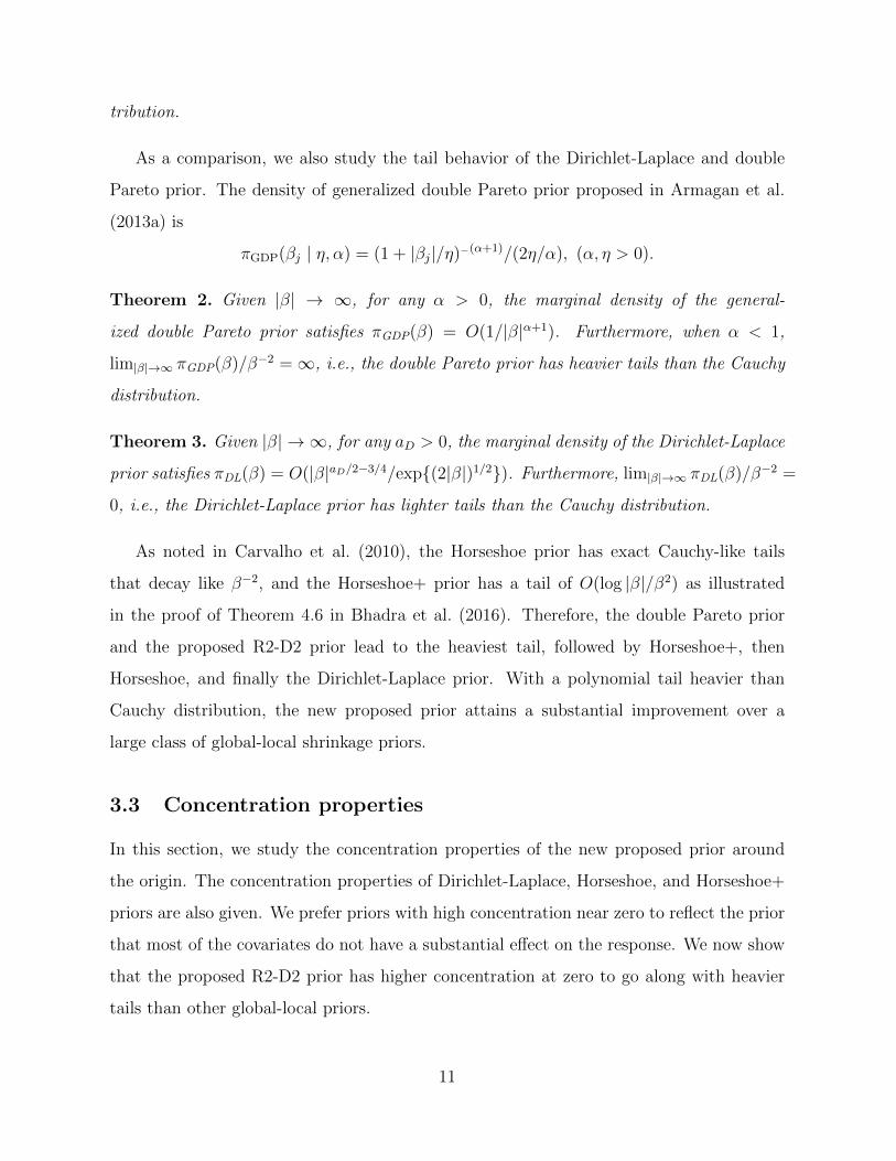
As a comparison, we also study the tail behavior of the Dirichlet-Laplace and double

Pareto prior. The density of generalized double Pareto prior proposed in Armagan et al.

(2013a) is

πGDP(βj | η, α) = (1 + |βj|/η)−(α+1)/(2η/α), (α, η > 0).

Theorem 2. Given |β| → ∞, for any α > 0, the marginal density of the general-

ized double Pareto prior satisfies πGDP(β) = O(1/|β|α+1). Furthermore, when α < 1,

lim|β|→∞ πGDP(β)/β−2 =∞, i.e., the double Pareto prior has heavier tails than the Cauchy

distribution.

Theorem 3. Given |β| → ∞, for any aD > 0, the marginal density of the Dirichlet-Laplace

prior satisfies πDL(β) = O(|β|aD/2−3/4/exp{(2|β|)1/2}). Furthermore, lim|β|→∞ πDL(β)/β−2 =

0, i.e., the Dirichlet-Laplace prior has lighter tails than the Cauchy distribution.

As noted in Carvalho et al. (2010), the Horseshoe prior has exact Cauchy-like tails

that decay like β−2, and the Horseshoe+ prior has a tail of O(log |β|/β2) as illustrated

in the proof of Theorem 4.6 in Bhadra et al. (2016). Therefore, the double Pareto prior

and the proposed R2-D2 prior lead to the heaviest tail, followed by Horseshoe+, then

Horseshoe, and finally the Dirichlet-Laplace prior. With a polynomial tail heavier than

Cauchy distribution, the new proposed prior attains a substantial improvement over a

large class of global-local shrinkage priors.

3.3 Concentration properties

In this section, we study the concentration properties of the new proposed prior around

the origin. The concentration properties of Dirichlet-Laplace, Horseshoe, and Horseshoe+

priors are also given. We prefer priors with high concentration near zero to reflect the prior

that most of the covariates do not have a substantial effect on the response. We now show

that the proposed R2-D2 prior has higher concentration at zero to go along with heavier

tails than other global-local priors.

11

Theorem 4. As |β| → 0, if 0 < aπ < 1/2, the marginal density of the R2-D2 prior (5)

satisfies πR2-D2(β) = O(1/|β|1−2aπ).

Theorem 5. As |β| → 0, if 0 < aD < 1, the marginal density of the Dirichlet-Laplace

prior satisfies πDL(β) = O(1/|β|1−aD).

For the Horseshoe prior, as summarized in Carvalho et al. (2010), the marginal density

πHS(β) = (2π3)−1/2 exp(β2/2)E1(β2/2), where E1(z) =∫∞

1e−tz/t dt is the exponential

integral function. As |β| → 0,

1

2(2π3)1/2log(1 +

4

β2) ≤ πHS(β) ≤ 1

(2π3)1/2log(1 +

2

β2).

Therefore around the origin, πHS(β) = O(log(1/|β|)). Also by the proof of Theorem 4.6

in Bhadra et al. (2016), as |β| → 0, the marginal density of Horseshoe+ prior satisfies

πHS+(β) = O(log2(1/|β|)). It is clear that 2aπ in the R2-D2 prior plays the same role

around origin as aD in the Dirichlet-Laplace prior. Accordingly, when aD = 2aπ ∈ (0, 1),

all these four priors possess unbounded density near the origin. However, the R2-D2 prior

and Dirichlet-Laplace prior diverge to infinity with a polynomial order, much faster than

the Horseshoe+ (with a squared logarithm order) and the Horseshoe prior (with a logarithm

order). Although the double Pareto prior also has a polynomial order tail similar as our

proposed R2-D2 prior, the double Pareto prior differs around the origin, as it remains

bounded, while our new proposed prior is unbounded at the origin.

Now we see that the R2-D2 prior and Dirichlet-Laplace prior put more mass in a small

neighborhood of zero compared to the Horseshoe and Horseshoe+ prior. Polson and Scott

(2010) established that when the truth is zero, a prior with unbounded density near zero is

super-efficient in terms of the Kullback-Leibler risk. As formalized below, the more mass

the prior puts around the neighborhood of the origin, the more efficient. Then the four

priors with unbounded density around zero are all super-efficient, with R2-D2 prior and

Dirichlet-Laplace more efficient than the Horseshoe+, and followed by Horseshoe. Section

3.5 discusses it in detail.

12

3.4 Posterior consistency

In this section, we show that the proposed R2-D2 prior yields posterior consistency. Assume

the true regression parameter is β0n, and the regression parameter βn is given some shrinkage

prior. If the posterior of βn converges in probability towards β0n, i.e., for any ε > 0,

pr(βn : ||βn − β0n|| > ε | Y) → 0 as pn, n → ∞, we say the prior yields a consistent

posterior.

Assume the following regularity conditions:

(A1) The number of predictors pn is o(n);

(A2) Let dpn and d1 be the smallest and the largest singular values of XTX/n respectively.

Assume 0 < dmin < lim infn→∞ dpn ≤ lim supn→∞ d1 < dmax < ∞, where dmin and

dmax are fixed and X = (xT1 , · · · ,xTn )T ;

(A3) lim supn→∞maxj=1,··· ,pn |β0nj| <∞;

(A4) qn = o(n/ log n), in which qn is the number of nonzero components in β0n.

Theorem 6. Under assumptions (A1)–(A4), for any b > 0, given the linear regression

model (1), and aπ = C/(pb/2n nρb/2 log n) for finite ρ > 0 and C > 0, the R2-D2 prior (5)

yields a consistent posterior.

3.5 Predictive efficiency

In this section, we study the predictive efficiency of the shrinkage priors. We focus on

the case when the design matrix X = (xT1 , · · · ,xTn )T is orthogonal, i.e., XTX = Ip. We

also assume σ2 to be known. Though this may not be a realistic setup in practice, it

provides some insight and motivation for measuring the predictive efficiency. In this case,

the sufficient statistic for β is the ordinary least square estimate, i.e., β = XTY, with

β ∼ N(β, σ2Ip). For simplicity of notation, without loss of generality, assume β0 is the

true parameter, we rewrite the sampling model as

yi ∼ N(β0, σ2) (8)

13

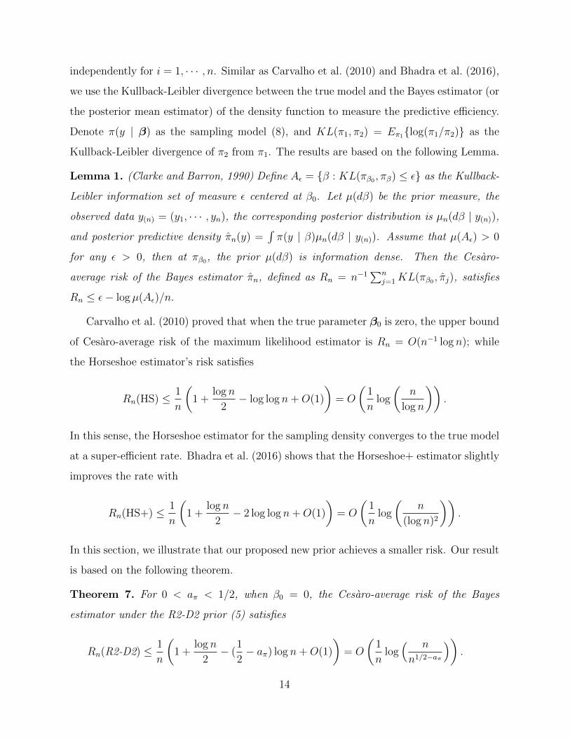
independently for i = 1, · · · , n. Similar as Carvalho et al. (2010) and Bhadra et al. (2016),

we use the Kullback-Leibler divergence between the true model and the Bayes estimator (or

the posterior mean estimator) of the density function to measure the predictive efficiency.

Denote π(y | β) as the sampling model (8), and KL(π1, π2) = Eπ1{log(π1/π2)} as the

Kullback-Leibler divergence of π2 from π1. The results are based on the following Lemma.

Lemma 1. (Clarke and Barron, 1990) Define Aε = {β : KL(πβ0 , πβ) ≤ ε} as the Kullback-

Leibler information set of measure ε centered at β0. Let µ(dβ) be the prior measure, the

observed data y(n) = (y1, · · · , yn), the corresponding posterior distribution is µn(dβ | y(n)),

and posterior predictive density πn(y) =∫π(y | β)µn(dβ | y(n)). Assume that µ(Aε) > 0

for any ε > 0, then at πβ0, the prior µ(dβ) is information dense. Then the Cesaro-

average risk of the Bayes estimator πn, defined as Rn = n−1∑n

j=1KL(πβ0 , πj), satisfies

Rn ≤ ε− log µ(Aε)/n.

Carvalho et al. (2010) proved that when the true parameter β0 is zero, the upper bound

of Cesaro-average risk of the maximum likelihood estimator is Rn = O(n−1 log n); while

the Horseshoe estimator’s risk satisfies

Rn(HS) ≤ 1

n

(1 +

log n

2− log log n+O(1)

)= O

(1

nlog

(n

log n

)).

In this sense, the Horseshoe estimator for the sampling density converges to the true model

at a super-efficient rate. Bhadra et al. (2016) shows that the Horseshoe+ estimator slightly

improves the rate with

Rn(HS+) ≤ 1

n

(1 +

log n

2− 2 log log n+O(1)

)= O

(1

nlog

(n

(log n)2

)).

In this section, we illustrate that our proposed new prior achieves a smaller risk. Our result

is based on the following theorem.

Theorem 7. For 0 < aπ < 1/2, when β0 = 0, the Cesaro-average risk of the Bayes

estimator under the R2-D2 prior (5) satisfies

Rn(R2-D2) ≤ 1

n

(1 +

log n

2− (

1

2− aπ) log n+O(1)

)= O

(1

nlog( n

n1/2−aπ

)).

14

As a complement, we also give the upper risk bounds for the DL prior:

Theorem 8. For 0 < aD < 1, when β0 = 0, the Cesaro-average risk of the Bayes estimator

under the Dirichlet-Laplace prior satisfies

Rn(DL) ≤ 1

n

(1 +

log n

2− (

1

2− aD

2) log n+O(1)

)= O

(1

nlog( n

n1/2−aD/2

)).

Therefore the R2-D2 prior and Dirichlet-Laplace priors have smaller Kullback-Leibler

risk bound than the Horseshoe and Horseshoe+ priors. Combining Theorems 1 and 4,

our proposed prior achieves desirable behavior both around the origin and in the tails, as

well as improved performance in prediction in the orthogonal case by Theorem 7. Table 1

provides the summary results of the above properties.

4 Simulation Study

To illustrate the performance of the proposed new prior, we conduct a simulation study with

various number of predictors and effect size. In each setting, 200 datasets are simulated

from the linear model (1) with σ2 = 1, sample size n fixed at 60 to match the real data

example in Section 5, and the number of predictors p varying in p ∈ {50, 100, 500}. The

covariates xi, i = 1, · · · , n, are generated from multivariate normal distribution with mean

zero, and correlation matrix of autoregressive (1) structure with correlation ρ =0.5 or 0.9.

For the regression coefficients β, we consider the following two setups.

Setup 1: β = (0T10,B1T ,0T30,B2

T ,0Tp−50)T with 0k representing the zero vector of length

k, and B1 and B2 each of length 5 nonzero elements. The fractions of true coefficients

with exactly zero values are 80%, 90% and 98% for p ∈ {50, 100, 500}, respectively, and the

remaining 20%, 10% and 2% nonzero elements B1 and B2 were independently generated

from a Student t distribution with 3 degrees of freedom to give heavy tails. In this case,

the theoretical R2 as in equation (2) is 0.97.

Setup 2: β = (0T10, s∗BT

3 ,0Tp−15)T with B3 also of length 5 with elements generated

independently from the Student t distribution with 3 degrees of freedom, with s∗ = 15−1/2

to ensure the total prior variance of β is 1 and hence the theoretical R2 as in equation (2)

15

is 0.5.

We consider p = 50, 100, 500 for setup 1, and only p = 100 for setup 2 because other

cases perform similarly. Setup 2 is designed to study the performance of the proposed R2-D2

prior with known R2 information. For each simulated dataset, we use different shrinkage

priors for β. The priors are Horseshoe, Horseshoe+, R2-D2(0.5,0.5) with a =0.5, b =0.5,

aπ = 1/(2p), R2-D2(p/n,0.5) with a = p/n, b =0.5, aπ = 1/n, R2-D2(p/n,0.1) with a = p/n,

b =0.1, aπ = 1/n, R2-D2(1,1) with a = 1, b = 1, aπ = 1/p, DL1/p with aD = 1/p, DL2/n

with aD = 2/n, and DL1/n with aD = 1/n. For the Horseshoe and Horseshoe+, Markov

chain Monte Carlo steps are implemented through Stan in R using the code provided by

the author of Bhadra et al. (2016). For the R2-D2 and Dirichlet-Laplace, Gibbs samplers

are implemented in R. 10, 000 samples are collected with the first 5, 000 samples discarded

as burn-in.

The average value of the sum squared error corresponding to the posterior mean across

the 200 replicates is provided in Table 2 with ρ =0.5. Simulation setup 1 with ρ =0.9

results are given in Table 3. Table 4 provides the results for simulation setup 2. Tables 2

and 4 give the total the sum squared error as well as the the sum squared error split into

three pieces according to the value of the true β at βj = 0, |βj| ∈ (0,0.5], and |βj| >0.5,

j = 1, · · · , p. The averaged area under the Receiver-Operating Characteristic curve based

on the posterior t-statistic, i.e., the ratio of the posterior mean and posterior standard

deviation, is also given to offer further evaluation of the variable selection performance.

We measure the reliability of the ordering of the magnitude of the posterior t-statistic

through the area under the Receiver-Operating Characteristic curve, which is labeled as

“ROC” in the tables.

Overall, the new proposed prior with a = p/n or aπ = 1/n has similar sum of squared

error to the Horseshoe and Horseshoe+ prior, and smaller than the Dirichlet-Laplace prior.

Horseshoe and Horseshoe+ yield good estimators with small sum of squared error. However,

Horseshoe and Horseshoe+ generally have lower Receiver-Operating Characteristic area,

worse than the R2-D2 prior and Dirichlet-Laplace priors. This may be explained by investi-

gating the sum of squared error for zero, small coefficients and large coefficients. Although

16

Horseshoe and Horseshoe+ estimate the nonzero coefficients quite well, they estimate the

zero coefficients poorly, which leads to more false positives and poor Receiver-Operating

Characteristic performance. This corresponds with the poor concentration properties of

the Horseshoe and Horseshoe+ as discussed in Section 3.3. In addition, we also conduct

simulations for fixed p with varying n, and the performance is similar.

Furthermore, the Dirichlet-Laplace priors exhibit excellent performance in estimating

the zero coefficients, but poor estimates of large coefficients, leading to large total sum

of squared error. This is due to the good concentration at the origin (Section 3.3) but

light tails of the Dirichlet-Laplace priors (Section 3.2). However, inaccurate estimation at

large coefficients does not greatly affect the Receiver-Operating Characteristic performance,

which is comparable to the R2-D2 priors. For the R2-D2 prior, the value of b slightly affects

the estimation. By analogy of the R2-D2 prior with a = p/n, b =0.5 and a = p/n, b =0.1,

we gain a key insight that a smaller value of b results in slightly smaller total sum of

squared error due to the better estimation at large coefficients. This coincides with the

fact that b controls the tail behavior (Section 3.2), with smaller b giving heavier tails. The

results show that a = 1 or aπ = 1/p and a =0.5 or aπ = 1/(2p) lead to smaller sum of

squared error at zero coefficients than a = p/n or aπ = 1/n when p > n, which again,

matches the concentration properties of R2-D2 prior as described in Section 3.3. There

is no significant difference in variable selection performance for the four parametrizations

in “R2-D2” prior. In all, the R2-D2 prior with aπ = 1/n and b <0.5 achieves success in

both estimation and variable selection, demonstrating distinguishable performance from

the Horseshoe, Horseshoe+ and Dirichlet-Laplace priors.

5 PCR Data Analysis

We now analyze the mouse gene expression data collected by Lan et al. (2006), consisting

of the expression levels of 22, 575 genes for n = 60 (31 female and 29 male) mice. Real-

time PCR was used to measure some physiological phenotypes, including number of phos-

phoenopyruvate carboxykinase (PEPCK), glycerol-3-phosphate acyltransferase (GPAT),

and stearoyl-CoA desaturase 1 (SCD1). We build regression models for the three phe-

17

notypes using gender and genetic covariates as predictors. The data can be found at

http://www.ncbi.nlm.nih.gov/geo; accession number GSE3330.

To evaluate the performance of different priors, the 60 observations are randomly split

into a training set of size 55 and testing set of size 5. Then in each split, the 22, 575

genes were first screened down to 999 genes based on the ordering of the magnitude of the

marginal correlation with the response only on the training data set with sample size 55.

Then for each of the 3 regressions, the data set contains p = 1, 000 predictors (999 genes

and gender) and n = 55 observations. After screening, we performed linear regression using

each of the global-local shrinkage prior. The convergence diagnostics plots of R2-D2 prior

are shown in Figure 2 and 3. Table 5 gives the mean squared prediction error based on

100 random splits of the data. The posterior mean of the regression coefficients from the

training set served as the estimate of β to make prediction for the testing set. Overall, the

results agree with the simulation studies. Our proposed R2-D2 prior performs better than

other priors for this data set, and changing the value of b has little effect on the results.

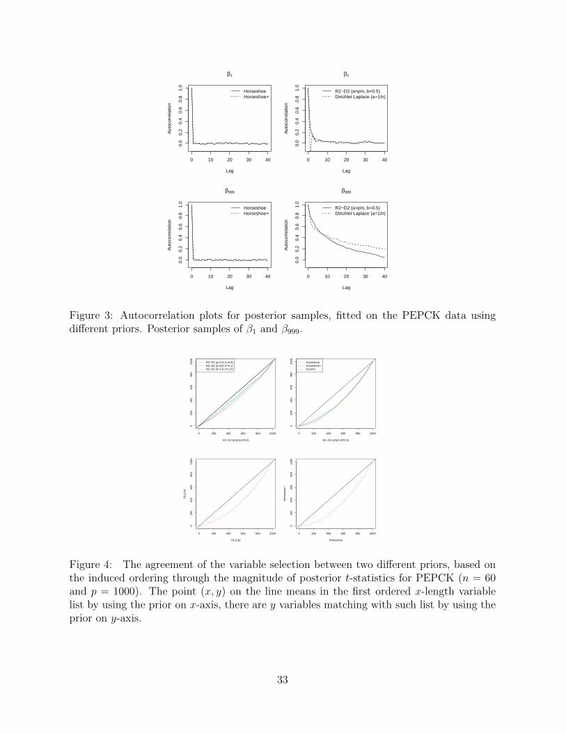
In addition, we also compared the agreement between methods in terms of variable

selection. For each regression, we apply different shrinkage priors on the full data set, then

posterior samples of β are collected. For each βj (j = 1, · · · , p), the posterior t-statistic

is calculated by dividing the mean with the standard deviation of those posterior samples.

The predictors are ordered by the magnitude of the posterior t-statistics from the largest

to the smallest. Ideally, the important predictors will be in the beginning of the ordering.

Figure 4 plots the agreement of the orders between various priors when fit to the full

data set for PEPCK. The figures for SCD1 and GPAT are similar. Again, it shows that

changing the value of b does not result in too much variation of the agreement. In general,

the difference of the agreement with different hyperparameter values in the R2-D2 priors

is smaller than that of Dirichlet-Laplace prior, and the difference between Horseshoe and

Horseshoe+ prior. For this data set, our proposed R2-D2 prior appears less sensitive to

different hyperparameter values than the Dirichlet-Laplace prior.

18

http://www.ncbi.nlm.nih.gov/geo

References

Armagan, A., Clyde, M., and Dunson, D. B. (2011). Generalized beta mixtures of Gaus-

sians. In Advances in neural information processing systems, pages 523–531.

Armagan, A., Dunson, D. B., and Lee, J. (2013a). Generalized double Pareto shrinkage.

Statistica Sinica, 23(1):119.

Armagan, A., Dunson, D. B., Lee, J., Bajwa, W. U., and Strawn, N. (2013b). Posterior

consistency in linear models under shrinkage priors. Biometrika, 100(4):1011–1018.

Bhadra, A., Datta, J., Polson, N. G., Willard, B., et al. (2016). The horseshoe+ estimator

of ultra-sparse signals. Bayesian Analysis.

Bhattacharya, A., Pati, D., Pillai, N. S., and Dunson, D. B. (2015). Dirichlet–Laplace priors

for optimal shrinkage. Journal of the American Statistical Association, 110(512):1479–

1490.

Bondell, H. D. and Reich, B. J. (2012). Consistent high-dimensional Bayesian variable

selection via penalized credible regions. Journal of the American Statistical Association,

107(500):1610–1624.

Carvalho, C. M., Polson, N. G., and Scott, J. G. (2009). Handling sparsity via the horseshoe.

In International Conference on Artificial Intelligence and Statistics, pages 73–80.

Carvalho, C. M., Polson, N. G., and Scott, J. G. (2010). The Horseshoe estimator for

sparse signals. Biometrika, page asq017.

Clarke, B. S. and Barron, A. R. (1990). Information-theoretic asymptotics of Bayes meth-

ods. Information Theory, IEEE Transactions on, 36(3):453–471.

DLMF (2015). NIST Digital Library of Mathematical Functions. http://dlmf.nist.gov/,

Release 1.0.10 of 2015-08-07. Online companion to Olver et al. (2010).

Fields, J. L. (1972). The asymptotic expansion of the Meijer G-function. Mathematics of

Computation, pages 757–765.

19

George, E. I. and McCulloch, R. E. (1993). Variable selection via Gibbs sampling. Journal

of the American Statistical Association, 88(423):881–889.

Griffin, J. E., Brown, P. J., et al. (2010). Inference with normal-gamma prior distributions

in regression problems. Bayesian Analysis, 5(1):171–188.

Hahn, P. R. and Carvalho, C. M. (2015). Decoupling shrinkage and selection in Bayesian

linear models: a posterior summary perspective. Journal of the American Statistical

Association, 110(509):435–448.

Ishwaran, H. and Rao, J. S. (2005). Spike and slab variable selection: Frequentist and

Bayesian strategies. Annals of Statistics, pages 730–773.

Johnson, N., Kotz, S., and Balakrishnan, N. (1995). Continuous univariate distributions,

volume 2. john wiley&sons. Inc.,, 75.

Lan, H., Chen, M., Flowers, J. B., Yandell, B. S., Stapleton, D. S., Mata, C. M., Mui, E.,

Flowers, M. T., Schueler, K. L., Manly, K. F., et al. (2006). Combined expression trait

correlations and expression quantitative trait locus mapping. PLoS Genet, 2(1):e6.

Miller, P. D. (2006). Applied asymptotic analysis, volume 75. American Mathematical Soc.

Mitchell, T. J. and Beauchamp, J. J. (1988). Bayesian variable selection in linear regression.

Journal of the American Statistical Association, 83(404):1023–1032.

Narisetty, N. N., He, X., et al. (2014). Bayesian variable selection with shrinking and

diffusing priors. The Annals of Statistics, 42(2):789–817.

Olver, F. W. J., Lozier, D. W., Boisvert, R. F., and Clark, C. W., editors (2010). NIST

Handbook of Mathematical Functions. Cambridge University Press, New York, NY. Print

companion to DLMF (2015).

Polson, N. G. and Scott, J. G. (2010). Shrink globally, act locally: Sparse Bayesian regu-

larization and prediction. Bayesian Statistics, 9:501–538.

20

Rockova, V. and George, E. I. (2016). The spike-and-slab lasso. Journal of the American

Statistical Association, (just-accepted).

Seshadri, V. (1997). Halphen’s laws. Encyclopedia of statistical sciences.

van der Pas, S., Salomond, J.-B., Schmidt-Hieber, J., et al. (2016). Conditions for poste-

rior contraction in the sparse normal means problem. Electronic Journal of Statistics,

10(1):976–1000.

Zhou, M. and Carin, L. (2015). Negative binomial process count and mixture modeling.

Pattern Analysis and Machine Intelligence, IEEE Transactions on, 37(2):307–320.

Zwillinger, D. (2014). Table of integrals, series, and products. Elsevier.

21

A Appendix

A.1 Technical details

Proof of Proposition 1. The proposition follows from

π(ω) =

∫ ∞0

π(ω | ξ)π(ξ)dξ =

∫ ∞0

ξa

Γ(a)ωa−1e−ξω

1

Γ(b)ξb−1e−ξdξ

=1

Γ(a)Γ(b)ωa−1

∫ ∞0

ξa+b−1e−(1+ω)ξdξ

=1

Γ(a)Γ(b)ωa−1 Γ(a+ b)

(1 + ω)a+b

=Γ(a+ b)

Γ(a)Γ(b)

ωa−1

(1 + ω)a+b(ω > 0).

Proof of Proposition 2 . The proposition follows from Lemma IV.3 of Zhou and Carin

(2015): Suppose y and (y1, · · · , yK) are independent with y ∼ Ga(φ, ξ), and (y1, · · · , yK) ∼

Dir(φp1, · · · , φpK), where∑K

k=1 pk = 1. Let xk = yyk, then xk ∼ Ga(φpk, ξ) independently

for k = 1, .sK.

Proof of Proposition 3 . The marginal density of β for the R2-D2 prior is

πR2-D2(β) =Γ(aπ + b)

Γ(aπ)Γ(b)

∫ ∞0

1

2(λ/2)1/2exp{− |β|

(λ/2)1/2} λaπ−1

(1 + λ)aπ+bdλ

=2aπΓ(aπ + b)

Γ(aπ)Γ(b)

∫ ∞0

exp(−|β|x)x2b

(x2 + 2)aπ+bdx.

Let µ = |β|, ν = b + 1/2, u2 = 2, and ρ = 1 − aπ − b, since |arg u| < π/2, Reµ > 0, and

22

Reν > 0, so we have

πR2-D2(β) =2aπΓ(aπ + b)

Γ(aπ)Γ(b)

∫ ∞0

exp(−µx)x2ν−1(x2 + u2)ρ−1 dx

=2aπΓ(aπ + b)

Γ(aπ)Γ(b)

u2ν+2ρ−2

2π1/2Γ(1− ρ)G31

13

(µ2u2

4

∣∣∣1−ν1−ρ−ν,0, 1

2

)(3.389.2 in Zwillinger (2014))

=2aπΓ(aπ + b)

Γ(aπ)Γ(b)

21/2−aπ

2π1/2Γ(aπ + b)G31

13

(β2

2

∣∣∣ 12−baπ− 1

2,0, 1

2

)=

1

(2π)1/2Γ(aπ)Γ(b)G31

13

(β2

2

∣∣∣ 12−baπ− 1

2,0, 1

2

)=

1

(2π)1/2Γ(aπ)Γ(b)G13

31

(2

β2

∣∣∣ 32−aπ ,1, 1212

+b

)

where G(.) denotes the Meijer G-Function, and the last equality follows from 16.19.1 in

DLMF (2015). Proposition 3 follows.

Proof of Theorem 1. For the proof of Theorem 1, we will use the following lemma found in

Miller (2006).

Lemma 2. (Watson’s Lemma) Suppose F (s) =∫∞

0e−stf(t) dt, f(t) = tαg(t) where g(t)

has an infinite number of derivatives in the neighborhood of t = 0, with g(0) 6= 0, and

α > −1. Suppose |f(t)| < Kect for any t ∈ (0,∞), where K and c are independent of t.

Then, for s > 0 and s→∞,

F (s) =n∑k=0

g(k)(0)

k!

Γ(α + k + 1)

sα+k+1+O(

1

sα+n+2).

According to equation (9) in the proof of Proposition 3, we have

πR2-D2(β) =2aπΓ(aπ + b)

Γ(aπ)Γ(b)

∫ ∞0

exp(−|β|x)x2b

(x2 + 2)aπ+bdx =

∫ ∞0

e−|β|xf(x) dx ≡ F (|β|),

where f(t) = C∗t2b/(t2 + 2)aπ+b ≡ t2bg(t), C∗ = 2aπΓ(aπ + b)/{Γ(aπ)Γ(b)}, and g(t) =

C∗(t2 + 2)−aπ−b with g(t) has an infinite number of derivatives in the neighborhood of

t = 0, with g(0) 6= 0. So the marginal density of R2-D2 prior is the Laplace transforms

of f(.). By Watson’s Lemma, since |f(t)| < Kect for any t ∈ (0,∞), where K and c are

23

independent of t, then as |β| → ∞,

F (|β|) =n∑k=0

g(k)(0)

k!

Γ(2b+ k + 1)

|β|2b+k+1+O(

1

|β|2b+n+2),

and setting n = 2 gives

F (|β|) = C∗{

2−aπ−bΓ(2b+ 1)

|β|2b+1+ 0

Γ(2b+ 2)

|β|2b+2+ (−aπ − b)2−aπ−b

Γ(2b+ 3)

|β|2b+3

}+O(

1

|β|2b+4)

= C∗2−aπ−b{

Γ(2b+ 1)

|β|2b+1− (aπ + b)

Γ(2b+ 3)

|β|2b+3

}+O(

1

|β|2b+4)

= O(1

|β|2b+1).

Hence, when b < 1/2, as |β| → ∞, we have

πR2-D2(β)1β2

= C∗2−aπ−b{

Γ(2b+ 1)

|β|2b−1− (aπ + b)

Γ(2b+ 3)

|β|2b+1+O(

1

|β|2b+2)

}→∞.

Proof of Theorem 2. It is obvious based on the marginal density of the generalized double

Pareto prior.

Proof of Theorem 3. According to 10.25.3 in DLMF (2015), when both ν and z are real,

if z → ∞, then Kν(z) ≈ π1/2(2z)−1/2e−z. Then as |β| → ∞, the marginal density of the

Dirichlet-Laplace prior given in Bhattacharya et al. (2015) satisfies

πDL(β) =1

2(1+aD)/2Γ(aD)|β|(aD−1)/2K1−aD((2|β|)1/2)

≈ 1

2(1+aD)/2Γ(aD)|β|(aD−1)/2π1/22−3/4|β|−1/4 exp{−(2|β|)1/2}

= C0|β|aD/2−3/4 exp{−(2|β|)1/2} = O(|β|aD/2−3/4

exp{(2|β|)1/2}),

where C0 = π1/22−3/4/{2(1+aD)/2Γ(aD)} is a constant value. Furthermore, as |β| → ∞,

πDL(β)

1/β2≈ C0|β|aD/2+5/4 exp{−(2|β|)1/2} → 0.

24

Proof of Theorem 4. For the proof of Theorem 4, we use the following lemma from Fields

(1972). Some useful notations used in the below proof: Denote aP = (a1, · · · , ap), as

a vector, similarly, bQ = (b1, · · · , bq), cM = (c1, · · · , cm), and so on. Let Γn(cP − t) =∏pk=n+1 Γ(ck−t), with Γn(cP −t) = 1 when n = p, Γ(cM−t) = Γ0(cM−t) =

∏mk=1 Γ(ck−t),

Γ∗(ai − aN) =∏n

k=1;k 6=i Γ(ai − ak), and

pFq

(aPbQ| w)

=∞∑k=0

Γ(aP + k)Γ(bQ)

Γ(bQ + k)Γ(aP )

wk

k!=∞∑k=0

p∏j=1

Γ(aj + k)q∏j=1

Γ(bj)

q∏j=1

Γ(bj + k)p∏j=1

Γ(aj)

wk

k!.

Lemma 3. (Theorem 1 in Fields (1972)) Given (i) 0 ≤ m ≤ q, 0 ≤ n ≤ p; (ii) ai − bkis not a positive integer for j = 1, · · · , p and k = 1, .s, q; (iii) ai − ak is not an integer for

i, k = 1, · · · , p, and i 6= k; and (iv) q < p or q = p and |z| > 1, we have

Gm,np,q

(z∣∣∣a1,··· ,apb1,··· ,bq

)=

n∑i=1

Γ∗(ai − aN)Γ(1 + bM − ai)Γn(1 + aP − ai)Γm(ai − bQ)

z−1+aiq+1Fp

(1,1+bQ−ai1+aP−ai

∣∣∣∣(−1)q−m−n

z

).

Now to prove Theorem 4, we have from Proposition 3 that, the marginal density of the

R2-D2 prior has πR2-D2(βj) = (2π)−1/2{Γ(aπ)Γ(b)}−1Gm,np,q (z|.) with m = 1, n = 3, p =

3, q = 1, a1 = 3/2− aπ, a2 = 1, a3 = 1/2, b1 = 1/2 + b, and z = 2/β2. Conditions (i)-(iv)

in Lemma 3 are satisfied for |β| near 0, since 0 < aπ < 1/2. Denote

C∗1 = (2π)−1/2(Γ(aπ)Γ(b))−1Γ(1

2− aπ)Γ(1− aπ)Γ(aπ)Γ(

1

2+ aπ) > 0

C∗2 = (2π)−1/2(Γ(aπ)Γ(b))−1Γ(aπ −1

2)Γ(

1

2)Γ(

1

2)Γ(

3

2− aπ) < 0

C∗3 = (2π)−1/2(Γ(aπ)Γ(b))−1Γ(aπ − 1)Γ(−1

2)Γ(

3

2)Γ(2− aπ) > 0

25

U1(β2) =∞∑k=0

Γ(aπ + b+ k)

Γ(12 + aπ + k)Γ(aπ + k)

(−1)k(β2

2 )k+aπ−1/2

k!≡∞∑k=0

(−1)ku1(k, β2)

U2(β2) =∞∑k=0

Γ(12 + b+ k)

Γ(32 − aπ + k)Γ(1

2 + k)

(−β2

2 )k

k!≡∞∑k=0

(−1)ku2(k, β2)

U3(β2) =∞∑k=0

Γ(1 + b+ k)

Γ(2− aπ + k)Γ(32 + k)

(−1)k(β2

2 )k+1/2

k!≡∞∑k=0

(−1)ku3(k,β2),

then

πR2-D2(β) =1

(2π)1/2Γ(aπ)Γ(b)G13

31

(2

β2

∣∣∣∣ 32−aπ,1, 1212+b

)

=1

(2π)1/2Γ(aπ)Γ(b)

3∑i=1

Γ∗(ai − aN )Γ(1 + bM − ai)Γ3(1 + aP − ai)Γ1(ai − bQ)

(2

β2)−1+ai

2F3

(1,1+bQ−ai1+aP−ai

∣∣∣∣−β2

2

)

=1

(2π)1/2Γ(aπ)Γ(b)

3∑i=1

3∏k=1;k 6=i

Γ(ai − ak)Γ(1 + b1 − ai)

3∏k=3+1

Γ(1 + ak − ai)1∏

k=1+1Γ(ai − bk)

(2

β2)−1+ai

2F3

(1,1+b1−ai1+aP−ai

∣∣∣∣−β2

2

)

=1

(2π)1/2Γ(aπ)Γ(b)

3∑i=1

3∏

k=1;k 6=iΓ(ai − ak)Γ(1 + b1 − ai)

1(

2

β2)−1+ai

∞∑k=0

Γ(1 + k)Γ(1 + b1 − ai + k)3∏j=1

Γ(1 + aj − ai)

3∏j=1

Γ(1 + aj − ai + k)Γ(1)Γ(1 + b1 − ai)

(−β2

2)k

k!

=

1

(2π)1/2Γ(aπ)Γ(b)

Γ(1

2− aπ)Γ(1− aπ)Γ(aπ + b)(

2

β2)12−aπ

∞∑k=0

Γ(1 + k)Γ(aπ + b+ k)Γ(1)Γ( 12

+ aπ)Γ(aπ)

Γ(1 + k)Γ( 12

+ aπ + k)Γ(aπ + k)Γ(aπ + b)

(−β2

2)k

k!

+Γ(aπ −1

2)Γ(

1

2)Γ(

1

2+ b)(

2

β2)0∞∑k=0

Γ(1 + k)Γ( 12

+ b+ k)Γ( 32− aπ)Γ(1)Γ( 1

2)

Γ( 32− aπ + k)Γ(1 + k)Γ( 1

2+ k)Γ( 1

2+ b)

(−β2

2)k

k!

+Γ(aπ − 1)Γ(−1

2)Γ(1 + b)(

2

β2)−

12

∞∑k=0

Γ(1 + k)Γ(1 + b+ k)Γ(2− aπ)Γ( 32

)Γ(1)

Γ(2− aπ + k)Γ( 32

+ k)Γ(1 + k)Γ(1 + b)

(−β2

2)k

k!

=

1

(2π)1/2Γ(aπ)Γ(b)

Γ(1

2− aπ)Γ(1− aπ)

∞∑k=0

Γ(aπ + b+ k)Γ( 12

+ aπ)Γ(aπ)

Γ( 12

+ aπ + k)Γ(aπ + k)

(−1)k(β2

2)k+aπ−1/2

k!

+Γ(aπ −1

2)Γ(

1

2)Γ(

1

2)

∞∑k=0

Γ( 12

+ b+ k)Γ( 32− aπ)

Γ( 32− aπ + k)Γ( 1

2+ k)

(−β2

2)k

k!

+Γ(aπ − 1)Γ(−1

2)Γ(

3

2)∞∑k=0

Γ(1 + b+ k)Γ(2− aπ)

Γ(2− aπ + k)Γ( 32

+ k)

(−1)k(β2

2)k+1/2

k!

≡

1

(2π)1/2Γ(aπ)Γ(b)

{Γ(

1

2− aπ)Γ(1− aπ)Γ(aπ)Γ(

1

2+ aπ)U1(β2) + Γ(aπ −

1

2)Γ(

1

2)Γ(

1

2)Γ(

3

2− aπ)U2(β2)

+Γ(aπ − 1)Γ(−1

2)Γ(

3

2)Γ(2− aπ)U3(β2)

}≡ C∗1U1(β2) + C∗2U2(β2) + C∗3U3(β2).

For fixed β near the neighborhood of zero, u1(k, β2), u2(k, β2), and u3(k, β2) are all mono-

tone decreasing, and converge to zero as k →∞. Thus, by alternating series test, U1(β2),

26

U2(β2), and U3(β2) all converge. Also, we have

C0|β|2aπ−1 − C1|β|2aπ+1 = u1(0, β2)− u1(1, β2) ≤ U1(β2) ≤ u1(0, β2) = C0|β|2aπ−1

C2 − C3|β|2 = u2(0, β2)− u2(1, β2) ≤ U2(β2) ≤ u2(0, β2) = C2

C4|β| − C5|β|3 = u3(0, β2)− u3(1, β2) ≤ U3(β2) ≤ u3(0, β2) = C4|β|,

where C0, C1, C2, C3, and C4 are all positive constants. So given that |β| in the neigh-

borhood of zero and aπ ∈ (0, 12),

C∗1 (C0|β|2aπ−1−C1|β|2aπ+1)+C∗2C2+C∗3 (C4|β|−C5|β|3) ≤ πR2-D2(β) ≤ C∗1C0|β|2aπ−1+C∗2 (C2−C3|β|2)+C∗3C4|β|,

then πR2-D2(β) = O(|β|2aπ−1).

Proof of Theorem 5. According to 10.30.2 in DLMF (2015), when ν > 0, z → 0 and z is

real, Kν(z) ≈ Γ(ν)(z/2)−ν/2. So given 0 < aD < 1 and |β| → 0,

πDL(β) =|β|(aD−1)/2K1−aD((2|β|)1/2)

2(1+aD)/2Γ(aD)≈|β|(aD−1)/2 1

2Γ(1− aD)( (2|β|)1/2

2)aD−1

2(1+aD)/2Γ(aD)= C|β|aD−1,

where C = Γ(1− aD)/21+aDΓ(aD) is a constant value. Theorem 5 follows then.

Proof of Theorem 6. Denote the estimated set of non-zero coefficients is An = {j : βnj 6=0, j = 1, · · · , pn}. Also σ2 is fixed at 1. Given the R2-induced Dirichlet decomposition

27

prior, the probability assigned to the region (βn : ||βn − β0n|| < tn) is

pr(βn : ||βn − β0n|| < tn) = pr

βn :∑j∈An

(βnj − β0nj)

2 +∑j 6∈An

β2nj < t2n

≥ pr

βj∈Annj :

∑j∈An

(βnj − β0nj)

2 <qnt

2n

pn

× pr

βj 6∈Annj :

∑j 6∈An

β2nj <

(pn − qn)t2npn

≥

∏j∈An

{pr

(βnj : |βnj − β0

nj | <tn

pn1/2

)}× pr

(βj 6∈Annj : β2

nj <t2npn

at least for one j

)

=∏

j∈An

{pr

(β0nj −

tnpn1/2

< βnj < β0nj +

tnpn1/2

)}×

[1−

{pr

(βj 6∈Annj : β2

nj ≥t2npn

)}pn−qn]

≥∏

j∈An

{pr

(− sup

j∈An|β0

nj | −tn

pn1/2< βnj < sup

j∈An|β0

nj |+tn

pn1/2

)}×

1−

{pr

(βj 6∈Annj : |βnj |b ≥

tbn

pb/2n

)}pn−qn

≥∏

j∈An

{pr

(− sup

j∈An|β0

nj | −tn

pn1/2< βnj < sup

j∈An|β0

nj |+tn

pn1/2

)}×

1−

{pb/2n E(|βnj |b)

tbn

}pn−qn

≥{

2tn

pn1/2π( sup

j∈An|β0

nj |+tn

pn1/2)

}qn

×

1−

{pb/2n E(|βnj |b)

tbn

}pn−qn ,

where π is the marginal density function of βj, symmetric and decreasing when the support

is positive, and the last but one “≥” is directly got from Markov’s inequality.

Also, based on prior (5), for any b > 0, conditional expectations give

E(|βj|b) = E[E{E(|βj|b | λj) | ξ}] = Eξ

[Eλj |ξ

{Γ(b+ 1)

(2/λj)b/2| ξ}]

=bΓ( b

2)Γ(aπ + b

2)

2b/2Γ(aπ).

Now assume tn = ∆/nρ/2 and assumptions (A1) – (A4) are satisfied. Then since

lim supj=1,··· ,pn |β0nj| <∞, there exists a sequence kn = o(n) such that supj=1,··· ,pn |β0

nj| < kn

and kn →∞ as n→∞. For the R2-D2 prior, based on equation (9), the marginal density is

a decreasing function on the positive supports. Then together with the tail approximation

of the marginal density as in the proof of Theorem 1, i.e., equation (9), we have

π( supj∈An|β0nj|+

tnpn1/2

) ≥ π(kn +tnpn1/2

) ≥ Γ(aπ + b)

Γ(aπ)Γ(b)2−b

Γ(2b+ 1)

(kn + ∆nρ/2pn1/2 )2b+1

.

Considering the fact that Γ(a) = a−1 − γ0 +O(a) for a close to zero with γ0 the Euler-

Mascheroni constant (see http://functions.wolfram.com/GammaBetaErf/Gamma/06/ShowAll.html),

28

now we have

pr(βn : ||βn − β0n|| <

∆

nρ/2)

≥

{2

∆

nρ/2pn1/2

Γ(aπ + b)

Γ(aπ)Γ(b)2−b

Γ(2b+ 1)

(kn + ∆nρ/2pn1/2 )2b+1

}qn

×

[1−

{pb/2n nρb/2bΓ( b

2)Γ(aπ + b

2)

∆b2b/2Γ(aπ)

}pn−qn]

≥

{2∆

nρ/2pn1/2

Γ(aπ + b)aπΓ(b)

2−bΓ(2b+ 1)

(kn + ∆nρ/2pn1/2 )2b+1

}qn

×

[1−

{pb/2n nρb/2bΓ( b

2)Γ(aπ + b

2)aπ

∆b2b/2

}pn−qn].

Taking the negative logarithm of both sides of the above formula, and letting aπ =

C/(pb/2n nρb/2 log n), we have

− log pr(βn : ||βn − β0n|| <

∆

nρ/2)

≤ −qn log

{2∆CΓ(aπ + b)2−bΓ(2b+ 1)

nρ/2pn1/2pb/2n nρb/2 log nΓ(b)

}+ qn(2b+ 1) log(kn +

∆

nρ/2pn1/2)

−qn log

[1−

{pb/2n nρb/2bΓ( b

2)Γ(aπ + b

2)C

∆b2b/2pb/2n nρb/2 log n

}pn−qn]

= −qn log

{2∆CΓ(aπ + b)2−bΓ(2b+ 1)

Γ(b)

}− qn log

[1−

{bΓ( b

2)Γ(aπ + b

2)C

∆b2b/2 log n

}pn−qn]+qn(2b+ 1) log(kn +

∆

nρ/2pn1/2) + qn log log n+

b+ 1

2qn log pn +

b+ 1

2qnρ log n

The dominating term is the last one, and if qn = o(n/ log n), − log pr(βn : ||βn − β0n|| <

∆/nρ/2) < dn for all d > 0, so pr(βn : ||βn − β0n|| < ∆/nρ/2) > exp(−dn). The posterior

consistency is completed by applying Theorem 1 in Armagan et al. (2013b).

Proof of Theorem 7. As shown in Theorem 4, when |β| is close to zero and 0 < aπ < 1/2,

πR2-D2(β) ≈ C1 + C2/β1−2aπ , where C1 and C2 are some constants, so

∫ n−1/2

0

πR2-D2(β) dβ ≈∫ n−1/2

0

(C1 +C2

β1−2aπ) dβ = n−1/2 C2

2aπ

(n

12−aπ + C1

2aπC2

).

29

By applying Lemma 1, we have

Rn(R2-D2) ≤ 1

n− 1

nlog

{1√n

C2

2aπ

(n

12−aπ + C1

2aπC2

)}≤ 1

n

{1 +

log n

2− log(n

12−aπ) +O(1)

}= O

(1

nlog( n

n1/2−aπ

)),

much smaller than the risk of the Horseshoe and Horseshoe+ prior, i.e., , O(log(n/(log n)b0

)/n),

where b0 is some constant value (note: b0 is different for Horseshoe and Horseshoe+

prior).

Proof of Theorem 8 . As shown in the proof of theorem 5, when |β| is close to zero and

0 < aD < 1, πDL(β) ≈ C|β|aD−1, where C = Γ(1− aD)/(21+aDΓ(aD)), so

∫ n−1/2

0

πDL(β) dβ ≈ C

∫ n−1/2

0

|β|aD−1 dβ =C

aDn−aD/2 =

C

aDn−1/2n

12−aD

2 .

By applying Lemma 1, we have

Rn(DL) ≤ 1

n− 1

nlog

(C

aDn−1/2n

12−aD

2

)≤ 1

n

{1 +

log n

2− log(n

12−aD

2 ) +O(1)

}= O

(1

nlog( n

n1/2−aD/2

)),

much smaller than the risk of the Horseshoe and Horseshoe+ prior, i.e., O(log{n/(log n)b0

}/n),

where b0 is some constant value (note: b0 is different for Horseshoe and Horseshoe+

prior).

A.2 Gibbs Sampling Procedures

Denote Z ∼ InvGaussian(µ, λ), if π(z) = λ1/2(2πz3)−1/2

exp{−λ(z − µ)2/(2µ2z)}. Denote

Z ∼ giG(χ, ρ, λ0), the generalized inverse Gaussian distribution (Seshadri, 1997), if π(z) ∝

zλ0−1exp{−(ρz + χ/z)/2}.

The Gibbs sampling procedure is as follows:

(a) Sample β|ψ,φ, ω, σ2,Y ∼ N(µ, σ2V), where µ = VXTY = (XTX + S−1)−1(XTY),

30

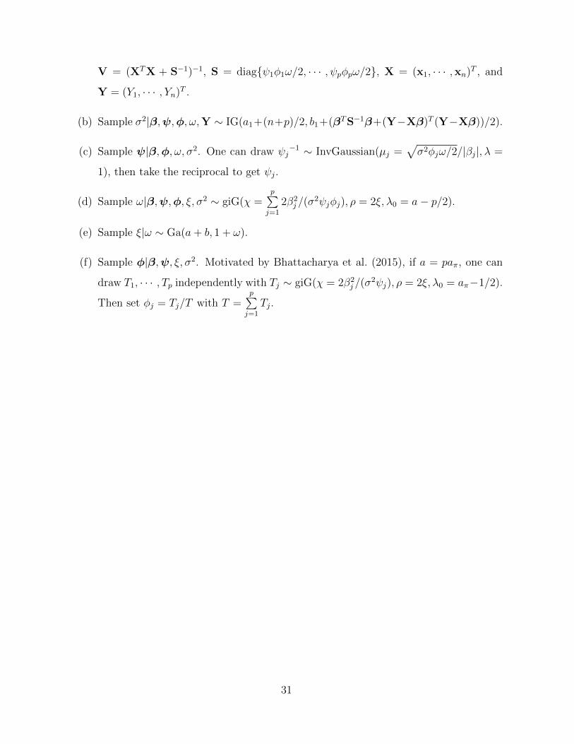
V = (XTX + S−1)−1, S = diag{ψ1φ1ω/2, · · · , ψpφpω/2}, X = (x1, · · · ,xn)T , and

Y = (Y1, · · · , Yn)T .

(b) Sample σ2|β,ψ,φ, ω,Y ∼ IG(a1+(n+p)/2, b1+(βTS−1β+(Y−Xβ)T (Y−Xβ))/2).

(c) Sample ψ|β,φ, ω, σ2. One can draw ψj−1 ∼ InvGaussian(µj =

√σ2φjω/2/|βj|, λ =

1), then take the reciprocal to get ψj.

(d) Sample ω|β,ψ,φ, ξ, σ2 ∼ giG(χ =p∑j=1

2β2j /(σ

2ψjφj), ρ = 2ξ, λ0 = a− p/2).

(e) Sample ξ|ω ∼ Ga(a+ b, 1 + ω).

(f) Sample φ|β,ψ, ξ, σ2. Motivated by Bhattacharya et al. (2015), if a = paπ, one can

draw T1, · · · , Tp independently with Tj ∼ giG(χ = 2β2j /(σ

2ψj), ρ = 2ξ, λ0 = aπ−1/2).

Then set φj = Tj/T with T =p∑j=1

Tj.

31

B Figures and Tables

−0.4 −0.2 0.0 0.2 0.4

0.0

0.5

1.0

1.5

2.0

2.5

3.0

β

Mar

gina

l den

sity

R2−D2CauchyHorseshoeHorseshoe+DL

5 10 15 20

0.00

00.

002

0.00

40.

006

0.00

80.

010

βM

argi

nal d

ensi

ty

R2−D2CauchyHorseshoeHorseshoe+DL

Figure 1: Marginal density of the R2-D2 (R2-D2), Dirichlet-Laplace (DL), Horseshoe,Horseshoe+ prior and Cauchy distribution. In all cases, the hyperparameters are selectedto ensure the inter quartile range is 1 for visual comparison.

0 2000 4000 6000 8000 10000

−1.

0−

0.5

0.0

0.5

Horseshoe

Index

β 1

0 2000 4000 6000 8000 10000

−1.

0−

0.5

0.0

0.5

Horseshoe+

Index

β 1

0 2000 4000 6000 8000 10000

−1.

0−

0.5

0.0

0.5

R2−D2 (a=p/n, b=0.5)

Index

β 1

0 2000 4000 6000 8000 10000

−1.

0−

0.5

0.0

0.5

Dirichlet Laplace (a=1/n)

Index

β 1

0 2000 4000 6000 8000 10000

−0.

50.

00.

51.

0

Horseshoe

Index

β 999

0 2000 4000 6000 8000 10000

−0.

50.

00.

51.

0

Horseshoe+

Index

β 999

0 2000 4000 6000 8000 10000

−0.

50.

00.

51.

0

R2−D2 (a=p/n, b=0.5)

Index

β 999

0 2000 4000 6000 8000 10000

−0.

50.

00.

51.

0

Dirichlet Laplace (a=1/n)

Index

β 999

Figure 2: Convergence plots for posterior samples, fitted on the PEPCK data using differentpriors. Posterior samples of β1 and β999.

32

0 10 20 30 40

0.0

0.2

0.4

0.6

0.8

1.0

β1

LagA

utoc

orre

latio

n

HorseshoeHorseshoe+

0 10 20 30 40

0.0

0.2

0.4

0.6

0.8

1.0

β1

Lag

Aut

ocor

rela

tion

R2−D2 (a=p/n, b=0.5)Dirichlet Laplace (a=1/n)

0 10 20 30 40

0.0

0.2

0.4

0.6

0.8

1.0

β999

Lag

Aut

ocor

rela

tion

HorseshoeHorseshoe+

0 10 20 30 40

0.0

0.2

0.4

0.6

0.8

1.0

β999

LagA

utoc

orre

latio

n

R2−D2 (a=p/n, b=0.5)Dirichlet Laplace (a=1/n)

Figure 3: Autocorrelation plots for posterior samples, fitted on the PEPCK data usingdifferent priors. Posterior samples of β1 and β999.

0 200 400 600 800 1000

020

040

060

080

010

00

R2−D2 (a=p/n,b=0.5)

R2−D2 (a=0.5, b=0.5)R2−D2 (a=p/n, b=0.1)R2−D2 (a=1.0, b=1.0)

0 200 400 600 800 1000

020

040

060

080

010

00

R2−D2 (a=p/n,b=0.5)

HorseshoeHorseshoe+DL(1/n)

0 200 400 600 800 1000

020

040

060

080

010

00

DL(1/p)

DL(

1/n)

0 200 400 600 800 1000

020

040

060

080

010

00

Horseshoe

Hor

sesh

oe+

Figure 4: The agreement of the variable selection between two different priors, based onthe induced ordering through the magnitude of posterior t-statistics for PEPCK (n = 60and p = 1000). The point (x, y) on the line means in the first ordered x-length variablelist by using the prior on x-axis, there are y variables matching with such list by using theprior on y-axis.

33

Table 1: Asymptotic properties for Horseshoe, Horseshoe+, R2-D2 (R2-D2) and Dirichlet-Laplace prior as discussed in Section 3

Tail Decay Concentration at zero Cesaro-average Risk Bound

Horseshoe O(

1β2

)O(

log( 1|β|))

O(

1n log

(n

logn

))Horseshoe+ O

(log |β|β2

)O(

log2( 1|β|))

O(

1n log

(n

(logn)2

))R2-D2 O

(1

|β|1+2b

)O(

1|β|1−2aπ

)O(

1n log

(n

n1/2−aπ

))Dirichlet-Laplace O

(|β|aD/2−3/4

exp{(2|β|)1/2}

)O(

1|β|1−aD

)O(

1n log

(n

n1/2−aD/2

))

34

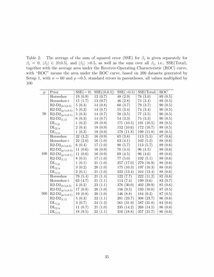
Table 2: The average of the sum of squared error (SSE) for βj is given separately forβj = 0, |βj| ∈ (0,0.5], and |βj| >0.5, as well as the sum over all βj, i.e., SSE(Total),together with the average area under the Receiver-Operating Characteristic (ROC) curve,with “ROC” means the area under the ROC curve, based on 200 datasets generated bySetup 1, with n = 60 and ρ =0.5, standard errors in parentheses, all values multiplied by100

p Prior SSE(= 0) SSE((0,0.5]) SSE(>0.5) SSE(Total) ROC

50

Horseshoe 19 (0.9) 12 (0.7) 48 (2.9) 78 (3.0) 89 (0.5)Horseshoe+ 15 (1.7) 13 (0.7) 46 (2.8) 74 (3.4) 89 (0.5)R2-D2(0.5,0.5) 5 (0.3) 14 (0.8) 60 (3.7) 79 (3.7) 90 (0.5)R2-D2(p/n,0.5) 5 (0.3) 14 (0.7) 55 (3.4) 74 (3.4) 90 (0.5)R2-D2(p/n,0.1) 5 (0.3) 14 (0.7) 58 (3.5) 77 (3.5) 90 (0.5)R2-D2(1,1) 6 (0.3) 14 (0.7) 54 (3.3) 74 (3.3) 90 (0.5)DL1/p 1 (0.2) 19 (0.9) 171 (10.5) 191 (10.5) 89 (0.5)DL2/n 2 (0.4) 18 (0.9) 152 (10.6) 172 (10.7) 89 (0.5)DL1/n 1 (0.3) 19 (0.9) 178 (11.8) 199 (11.8) 89 (0.5)

100


500


35

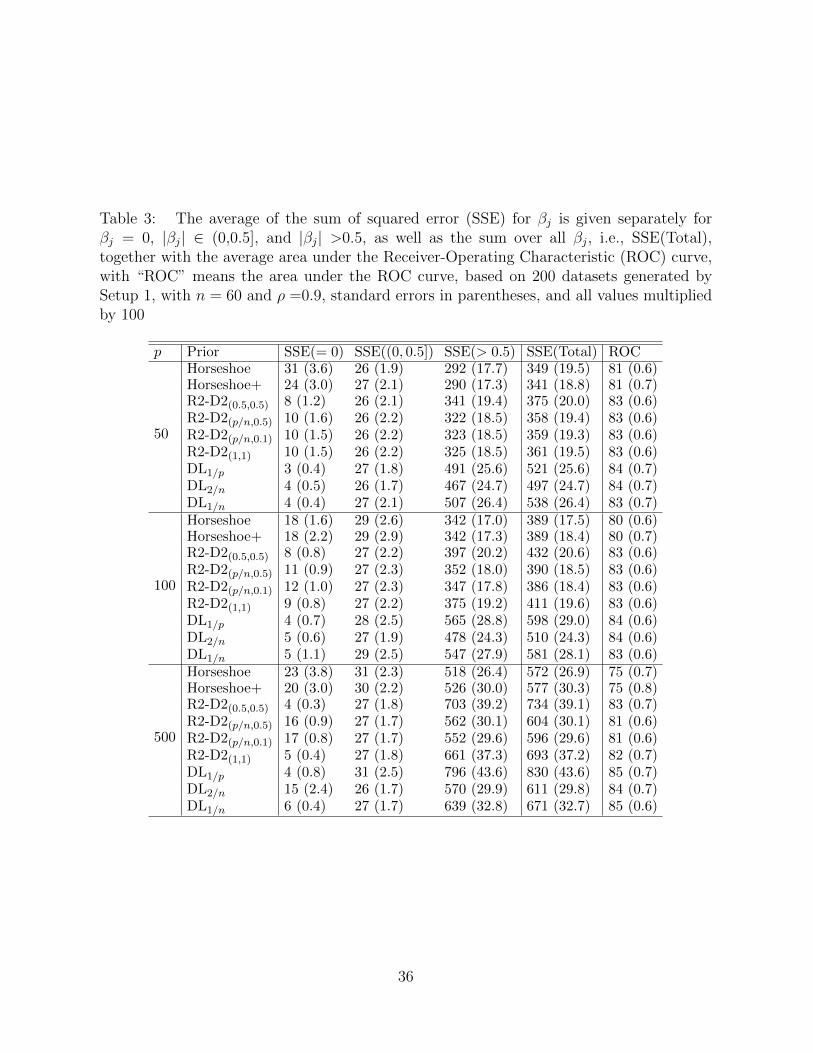
Table 3: The average of the sum of squared error (SSE) for βj is given separately forβj = 0, |βj| ∈ (0,0.5], and |βj| >0.5, as well as the sum over all βj, i.e., SSE(Total),together with the average area under the Receiver-Operating Characteristic (ROC) curve,with “ROC” means the area under the ROC curve, based on 200 datasets generated bySetup 1, with n = 60 and ρ =0.9, standard errors in parentheses, and all values multipliedby 100

p Prior SSE(= 0) SSE((0, 0.5]) SSE(> 0.5) SSE(Total) ROC

50


100


500


36

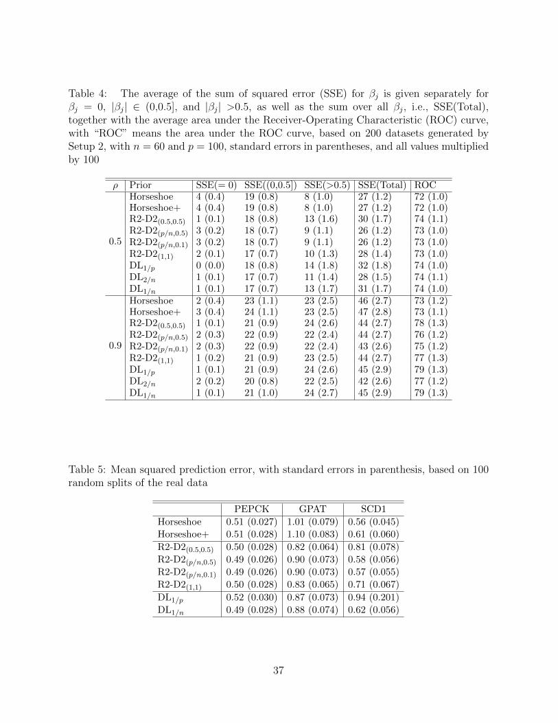
Table 4: The average of the sum of squared error (SSE) for βj is given separately forβj = 0, |βj| ∈ (0,0.5], and |βj| >0.5, as well as the sum over all βj, i.e., SSE(Total),together with the average area under the Receiver-Operating Characteristic (ROC) curve,with “ROC” means the area under the ROC curve, based on 200 datasets generated bySetup 2, with n = 60 and p = 100, standard errors in parentheses, and all values multipliedby 100

ρ Prior SSE(= 0) SSE((0,0.5]) SSE(>0.5) SSE(Total) ROC

0.5


0.9


Table 5: Mean squared prediction error, with standard errors in parenthesis, based on 100random splits of the real data

PEPCK GPAT SCD1

Horseshoe 0.51 (0.027) 1.01 (0.079) 0.56 (0.045)Horseshoe+ 0.51 (0.028) 1.10 (0.083) 0.61 (0.060)

R2-D2(0.5,0.5) 0.50 (0.028) 0.82 (0.064) 0.81 (0.078)

R2-D2(p/n,0.5) 0.49 (0.026) 0.90 (0.073) 0.58 (0.056)

R2-D2(p/n,0.1) 0.49 (0.026) 0.90 (0.073) 0.57 (0.055)

R2-D2(1,1) 0.50 (0.028) 0.83 (0.065) 0.71 (0.067)

DL1/p 0.52 (0.030) 0.87 (0.073) 0.94 (0.201)

DL1/n 0.49 (0.028) 0.88 (0.074) 0.62 (0.056)

37

high dimensional linear regression via the r2-d2 … dimensional linear regression via the r2-d2 ......

Documents