high-frequency planetary waves in the polar … ozone wave in the assimilation system is in good...
TRANSCRIPT

15 DECEMBER 2003 2975C O Y E T A L .
q 2003 American Meteorological Society
High-Frequency Planetary Waves in the Polar Middle Atmosphere as Seen in a DataAssimilation System
L. COY
E. O. Hulburt Center for Space Research, Naval Research Laboratory, Washington, D.C.
I. STAJNER, A. M. DASILVA, J. JOINER, R. B. ROOD, S. PAWSON, AND S. J. LIN
NASA Goddard Space Flight Center, Greenbelt, Maryland
(Manuscript received 29 January 2003, in final form 18 July 2003)
ABSTRACT
The 4-day wave often dominates the large-scale wind, temperature, and constituent variability in the high-latitude Southern Hemisphere winter near the stratopause. This study examines the winter Southern Hemispherevortex of 1998 using 4-times-daily output from a data assimilation system to focus on the polar 2-day, wave-number-2 component of the 4-day wave. The data assimilation system products are from a test version of thefinite volume data assimilation system (fvDAS) being developed at the Goddard Space Flight Center (GSFC)and include an ozone assimilation system. Results show that the polar 2-day wave in temperature and ozonedominates over other planetary-scale disturbances during July 1998 at 708S. The period of the quasi-2-day waveis somewhat shorter than 2 days (about 1.7 days) during July 1998 with an average perturbation temperatureamplitude for the month of over 2.5 K. The 2-day wave propagates more slowly than the zonal mean zonalwind, consistent with Rossby wave theory, and has Eliassen–Palm (EP) flux divergence regions associated withregions of negative horizontal potential vorticity gradients, as expected from linear instability theory. Resultsfor the assimilation-produced ozone mixing ratio show that the 2-day wave represents a major source of ozonevariation in this region. The ozone wave in the assimilation system is in good agreement with the wave seenin the Polar Ozone and Aerosol Measurement (POAM) ozone observations for the same time period. Somedifferences from linear instability theory are noted, as well as spectral peaks in the ozone field, not seen in thetemperature field, that may be a consequence of advection.
1. Introduction
The 4-day wave is a relatively common planetary-scale stratopause disturbance found mainly during theSouthern Hemisphere winter. This high-latitude waveconsists of wavenumber-1 (wave 1) and wavenumber-2 (wave 2) (and some higher wavenumber) componentsmoving at nearly the same rotational period (the timefor a crest to travel around a latitude circle), about 3–4 days, so that the period of the wave-2 component isabout 1.5–2 days. Many studies of the 4-day wave havefocused on the wave-1 component because only dailyanalyses are needed to resolve the period accurately.However, modern data assimilation systems that includethe stratosphere often output 4 times a day and so canbe used to examine the higher-frequency wave-2 com-ponent of the 4-day wave. This paper presents resultsof the 4-day wave seen in the temperature and ozonefields produced by a global data assimilation system
Corresponding author address: Lawrence Coy, E. O. Hulburt Cen-ter for Space Research, Naval Research Laboratory, Code 7646, 4555Overlook Avenue SW, Washington, DC 20375-5320.E-mail: [email protected]
during a time when the wavenumber-2 component wasdominant.
The 4-day wave has been described by Venne andStanford (1979, 1982), Prata (1984), Lait and Stanford(1988), Randel and Lait (1991), Manney (1991), Lawr-ence et al. (1995), and Lawrence and Randel (1996);more references can be found in Allen et al. (1997).Most of these studies examined satellite radiances,though Manney (1991) used daily analyses provided bythe National Centers for Environmental Prediction(NCEP), that combined data assimilation products inthe troposphere (at and below 100 hPa) with objectiveanalysis products in the stratosphere (above 100 hPa).The wave originates near the stratopause at the level ofthe stratospheric jet maximum where the latitudial meanzonal wind shears tend to be largest. The wave is be-lieved to be generated by barotropic and baroclinic in-stability, the relative importance of either process de-pending on the particular zonal mean wind configura-tion. The wave is of interest because it is often thedominant large-scale dynamical feature in the high-lat-itude Southern Hemisphere winter near the stratopause,perturbing temperatures, constituents, and winds.

2976 VOLUME 60J O U R N A L O F T H E A T M O S P H E R I C S C I E N C E S
The linear barotropic instability problem at the stra-topause germane to 4-day wave genesis was first in-vestigated by Hartmann (1983) for idealized latitudinalzonal wind profiles. Hartmann (1983) found that insta-bilities could occur on both the poleward and equator-ward side of jets corresponding to negative zonal meanpotential vorticity gradients on both sides of the jet. Thezonal phase speeds of the unstable waves were nearlyequal to the mean zonal wind speed where y (the zonalqmean potential vorticity gradient) changed sign. Thisgives shorter rotational periods on the poleward side ofthe jet (;4 days) and longer rotational periods on theequatorward side of the jet (;15 days) because of thechange in length of latitude circles around the globe,even though the phase speeds could be similar on bothsides of the jet. Using a quasigeostrophic model, Hart-mann (1983) also found that baroclinic effects tendedto stabilize and reduce growth rates by confining thevertical extent of the region of strong latitudinal windshear. In Hartmann (1983) both wavenumbers 1 and 2had similar growth rates; however, another barotropicmodel study (Manney et al. 1988) showed that wave 2became the more unstable mode (rather than wave 1)as the jet became more sharply peaked. Manney et al.(1988) also showed that the waves became more dis-persive (i.e., the rotational period had more variationfor different wavenumbers) as the jet moved equator-ward.
Manney and Randel (1993) used a linear quasigeo-strophic model to examine unstable modes in climato-logical zonal mean winds, including both barotropic andbaroclinic effects. They showed that both effects werenecessary for realistic growth rates to occur in the zonalmean winds they studied. These results agreed with ob-servational studies (Randel and Lait 1991) that showedstrong vertical Eliassen–Palm (EP) fluxes (a baroclinicsignature) in some 4-day wave observations. More re-cent work by Allen et al. (1997) highlighted the generalstructure of the 4-day wave in terms of the temperatures,winds, and heights associated with a potential vorticity(PV) anomaly.
Stratospheric constituents can respond to the 4-daywave as tracers if they have mean gradients in the waveregion and relatively long chemical lifetimes. Usinghigh-latitude middle-atmosphere observations from theUpper Atmosphere Research Satellite (UARS) Allen etal. (1997) showed a 4-day signal in ozone, while Man-ney et al. (1998) showed a 4-day signal in water vaporand methane. Both studies modeled the tracers differ-ently. Allen et al. (1997) calculated the linear ozoneresponse to the observed temperature and geostrophicmeridional wind signal coupled with simple photo-chemistry to examine the vertical structure of the ozonesignal. Manney et al. (1998) used an isentropic transportmodel to examine tracer transport associated with the4-day wave. Both studies showed that the 4-day wave,when active, can explain a large amount of the tracervariability near the polar stratopause.
This paper reports on the higher-frequency, wave-2component of the 4-day wave using 6-hourly outputfrom a data assimilation system that includes outputfrom an offline ozone assimilation, as well as the stan-dard assimilation-produced mass and wind fields. Fol-lowing a brief description of the assimilation productsand analysis methods (section 2), the assimilation-based4-day wave diagnostics are presented (section 3). Inaddition to the ozone assimilation, the 4-day wave canbe seen in Polar Ozone and Aerosol Measurement(POAM) observations (section 4). Discussion and con-clusions follow in sections 5 and 6, respectively.
2. Analysis
This study uses assimilated products produced by theNational Aeronautics and Space Administration’s(NASA) Data Assimilation Office (DAO), includingoutput from a meteorological data assimilation system(DAS) and an offline ozone data assimilation system(O3DAS). The analysis in this study was performedusing 6-hourly output from both of these assimilateddatasets for 1998. These assimilation products provideglobally gridded fields of temperature, winds, andozone, at regular time intervals, by incorporating ob-servations into a general circulation model. The advan-tages of using assimilated datasets over raw observa-tions for this study include a global grid, better verticalresolution than unprocessed radiance measurements,and dynamically consistent winds and temperatures,suitable for calculating higher-order dynamical quati-ties.
Meteorological analyses are from a prototype versionof NASA’s Goddard Earth Observing System version 4(GEOS-4) DAS, which is referred to as the finite-vol-ume DAS (fvDAS). The same dataset was used byDouglass et al. (2003) and Schoeberl et al. (2003) instudies of transport, mainly in the lower stratosphere.The fvDAS uses the Physical-Space Statistical AnalysisScheme (PSAS; Cohn et al. 1998) and a state-of-the-art general circulation model, the fvGCM. The fvGCMis based on the flux-form semi-Lagrangian dynamicalcore of Lin and Rood (1996, 1997) and Lin (1997),coupled to the Community Climate Model version 3(CCM) physics of Kiehl et al. (1988). The model in-cludes a hybrid sigma-pressure vertical coordinate with55 levels, the upper boundary being at 0.01 hPa. Eventhough the model extends well into the mesosphere, themeteorological dataset from the fvDAS has no data con-straints at pressures lower than 0.4 hPa. This dataset isthus useful for studies from the surface to the lowermesosphere.
The data constraint at the levels of interest for thisstudy comes from the Television Infrared ObservationSatellite (TIROS) Operational Vertical Sounder (TOVS)radiances, assimilated in a one-dimensional variational(1DVAR) procedure described by Joiner and Rokke(2000). Until July 1998, data from the National Oceanic

15 DECEMBER 2003 2977C O Y E T A L .
and Atmospheric Administration’s NOAA-11 andNOAA-14 TOVS were assimilated. TOVS consists ofthe High Resolution Infrared Sounder (HIRS), a 20-channel IR filter-wheel radiometer; a stratosphericsounding unit (SSU), a three-channel radiometer thatuses a pressure-modulation technique; and a microwavesounding unit (MSU), a four-channel microwave radi-ometer. The channels affecting the upper stratosphereare the two highest peaking SSU channels and HIRSchannel 1. To avoid intersatellite biases (upper-strato-spheric channels are not bias corrected), the NOAA-11SSU channels were not assimilated. After 1 July 1998,data from the NOAA-15 Advanced TOVS (ATOVS)were added to the assimilation, where the 15-channelAdvanced Microwave Sounding Unit (AMSU) replacedthe SSU and MSU of previous NOAA satellites. Toavoid intersatellite bias between the NOAA-15 ATOVSand the NOAA-14 SSU, the NOAA-14 SSU channelswere not assimilated after 1 July 1998.
Meteorological output fields from the fvDAS wereused to drive the transport model in the DAO’s O3DAS(Stajner et al. 2001). This offline assimilation uses totalcolumn ozone from the Total Ozone Mapping Spec-trometer (TOMS) instrument in conjunction with coarseprofile information from the Solar Backscattered Ultra-violet (SBUV) instrument. The assimilation is per-formed on a vertical grid with 29 levels spanning thesurface to 0.2 hPa, with 9 levels in the troposphere and20 levels in the stratosphere. Note that the fvGCM useda zonally averaged ozone climatology for its radiativeheating calculations, not the three-dimensional ozoneassimilation that was run offline. Thus, there is no feed-back between the ozone and dynamics.
Both the fvDAS and O3DAS were run, for this study,with a horizontal resolution of 28 latitude 3 2.58 lon-gitude. For the analysis performed here, data were in-terpolated to 36 pressure levels spanning 1000 to 0.2hPa. Zonal and meridional winds, temperature, and geo-potential height from the fvDAS were analyzed along-side the ozone.
A standard Fourier transform package was used ontwo-dimensional longitude by time arrays to extract theeastward-propagating wave components of interest at agiven latitude and height. The Fourier analysis was per-formed monthly (120–124 points in time). The west-ward-propagating modes consist mainly of solar tidalperiods and are not shown here. Though some higher-wavenumber components also show the 4-day wave,only the dominant wave-1 and wave-2 components arepresented here. Eliassen–Palm fluxes and associatedheat and momentum fluxes were calculated for a givenwavenumber and frequency from the zonal wind, me-ridional wind, and temperature Fourier coefficientsalong with the zonally and monthly averaged zonalwinds and temperatures. The EP flux formulas wereevaluated using spherical, log-pressure coordinates [seeAndrews et al. 1987, Eq. (3.5.3a,b), p. 128].
Since plots of EP flux and EP flux divergence will
be presented in section 3, a brief review of pertinentequations based on Andrews et al. (1987, sections 3.5and 3.6) is given here. The EP flux divergence representsthe wave forcing of the zonal mean zonal wind in thetransformed Eulerian-mean zonal momentum equation[Andrews et al. 1987, Eq. (3.5.2a), p. 128]. The EP fluxdivergence is also a term in a wave conservation equa-tion:
]A31 = · F 5 D 1 O(a ), (1)
]t
[Andrews et al. 1987, Eq. (3.6.2), p. 131], where A isthe wave-activity density, D depends on frictional anddiabatic effects, and O(a3) represents nonlinear waveeffects. As pointed out in Andrews et al. (1987), A andD depend in a complicated way on particle displace-ments. This limits the usefulness of Eq. (1) in general;however, a time average of Eq. (1) shows that the time-averaged EP flux divergence pattern must be balancedby the time average of the frictional, diabatic, and non-linear terms.
The quasigeostropic beta-plane version of Eq. (1) isgiven by
2] 1 r q9 r Z9q90 0 31 = · F 5 1 O(a ), (2)1 2]t 2 q qy y
[Andrews et al. 1987, Eq. (3.6.5), p. 132], where q isthe quasigeostrophic potential vorticity, and Z containsboth frictional and diabatic terms. The EP flux diver-gence, = ·F, is now the quasigeostropic EP flux diver-gence on the beta plane. The prime denotes the deviationfrom zonal average. Equation (2) can be used to relatethe EP flux divergence to linear instability studies,where the right-hand side is neglected so that, for grow-ing wave modes, = ·F will be positive (divergent) inregions of negative y and negative (convergent) in re-qgions of positive y.q
3. Results
The 4-day wave can be seen in the gridded assimi-lation products. Figure 1 shows longitude time sectionsfor temperature and ozone mixing ratio at 708S and 2hPa for July 1998. Both fields show wavenumber-2 fea-tures propagating eastward with periods of about 2 days.The peak-to-peak amplitude is on the order of 10 K fortemperature and 1 ppmv for ozone. A comparison withindependent POAM ozone observations will be givenlater.
Figure 2 gives a representitive mid-July 2-hPa syn-optic view of the South Pole where the wave-2 structurecan be seen. The temperature field (Fig. 2a) shows twowarm regions with a cold, elongated region in between,located over the pole. Both of these warm regions arealso seen in the Met Office stratospheric assimilation(not shown) so the warm regions are unlikely to be aDAO system artifact. However, there are differences in

2978 VOLUME 60J O U R N A L O F T H E A T M O S P H E R I C S C I E N C E S
FIG. 1. Longitude–time plot of (a) temperature (K) and (b) ozonemixing ratio (ppmv) at 708S and 2 hPa for Jul 1998. Temperaturecontour interval is 5 K. Cooler temperatures are shaded. Ozone con-tour interval is 1 ppmv. Lower ozone values are shaded.
temperatures between the two analyses that reflect thedifficulties still associated with temperature analysesnear the stratopause. The Ertel PV field (Fig. 2b) showsa strong gradient associated with the main polar vortexand a weaker inner vortex associated with the wave-number-2 feature. Ozone (Fig. 2c) also shows an elon-gated wave-2 low-ozone region near the pole. The phaseof the ozone wave disturbance is somewhat east of thetemperature and PV waves. In addition, the zonal windcomponent (Fig. 2d) shows a wave-2-shaped region ofweak winds over the Pole. The zonal wind is of interestbecause its meridional derivative can help to create thenegative regions of potential vorticity gradient qy neededfor instability of the zonal flow. Negative regions ofquasigeostrophic potential vorticity gradient are shadedin Fig. 2d. The three negative regions associated withthe inner vortex change with time as the fast inner vortexinteracts with the slower changing main vortex. Thoughthis paper focuses on the waves interacting with a zon-ally averaged basic state, the complicated negative qy
pattern, with its lack of zonal symmetry, should be kept
in mind. In addition to wave 2, the patterns in Fig. 2show a wave-1 component as well, in that the distur-bance is centered somewhat off the Pole; however, thewave-2 feature stands out more clearly at this time.
A representative 6-month time series (April–Septem-ber 1998) of temperature and ozone at a point at 708Sand 2 hPa (Fig. 3) shows 2–4-day fluctuations through-out the time period. The temperature and ozone oscil-lations increase in amplitude during July 1998, thoughthe ozone shows larger-amplitude disturbances thantemperature in May and June. There is some evidencehere (verified by spectral analysis) that the period of theoscillations is higher in July than in August. This cor-responds to dominance of wave 2 over wave 1 in Julyshown below.
Figure 4 shows the zonally averaged temperature andozone at 2 hPa as a function of time and latitude. Whilethe ozone gradients increase somewhat with time, thetemperature structure changes dramatically in July 1998,with a relatively warm region forming at 608–708S andincreased meridional temperature gradients poleward of708S. These temperature changes are related to the sea-sonal downward motion of the wintertime jet and for-mation of a double jet near the stratopause. As will beshown, this warm region is where the wave-2 compo-nent of the 4-day wave is found.
The following figures highlight the month of July1998 because spectral analysis of the months May–Sep-tember 1998 (not shown) revealed that the wavenumber-2 component was much larger than the wavenumber-1component during July.
Figure 5a shows the zonal mean zonal wind for themonth of July 1998 and its associated negative regionof y. The jet tilts strongly equatorward with altitudeqwith a weak poleward secondary maximum at the up-permost levels. In between the two jets is the negative
y region. The critical line for the 0.58 day21 waveq(described in more detail below) and the y 5 0 lineqcoincide at upper levels, in the region between the twojets. The reference level at 0.4 hPa shows how therecan be three critical levels at a given altitude. Figure5b shows the zonal mean temperatures for July 1998.The dashed line shows where the meridional tempera-ture gradient is zero. A region of reversed temperaturegradient (warm air toward the pole) extends from themesosphere down into the stratosphere. As will beshown, this region is where the temperature perturbationwave-2 component of the 4-day wave has a maximum.The possible significance of this reversed temperaturegradient region is discussed in section 6.
Figure 6 shows the July 1998 eastward-propagatingtemperature and ozone frequency spectrum as a functionof pressure at 708S for wave 1 and wave 2. Also plottedis the critical line, derived from the zonal mean zonalwind, for each frequency and wavenumber. Note thatmost wave activity is bounded by the critical line in-dicating that the waves are regressing with respect tothe zonal mean winds as expected for Rossby waves.

15 DECEMBER 2003 2979C O Y E T A L .
FIG. 2. Circulation at 2 hPa at 1200 UTC 16 Jul 1998: (a) temperature (K), temperatures less than 235 K shaded,contour interval 2.5 K; (b) potential vorticity (PVU, where 1 PVU 5 1 3 1026 K m2 kg21 s21), PV less than 25500PVU shaded, contour interval 500 PVU; (c) ozone (ppmv), ozone less than 2.5 ppmv shaded, contour interval 0.5ppmv; and (d) zonal wind component (m s21), qy less than zero is shaded, contour interval 10 m s21. Orthographicprojection from the equator to the South Pole, 908E at the bottom of the plots, highlighted latitude at 708S.
The wave-1 temperature spectra (Fig. 6a) are large forthe stationary and slowly propagating waves; howeverthe amplitudes are relatively weak and poorly definednear the 4-day wave frequency (0.25 day21). The wave-1 ozone spectra (Fig. 6b) show a stationary wave peakat 2 hPa and a weak ozone peak at a fairly high period(0.4 day21) very near the critical line. The wave-2 tem-perature spectra (Fig. 6c) show a large, vertically co-herent peak at about 0.6 day21. This is the wave-2 struc-ture; the period is about 1.7 days. The spectral peakmaximizes between 1–2 hPa and extends from the topof the domain down to the critical line. The wave-2ozone spectra (Fig. 6d) shows a similar 0.6 day21 peak,though it is much more localized in the vertical thanthe wave-2 temperature peak. Ozone also tends to show
a weak peak at higher frequencies near the critical line,similar to the wave-1 ozone spectra.
The same frequencies as a function of latitude, at 2hPa, are shown in Fig. 7. Once again the waves aregenerally constrained by the critical line to be propagat-ing more slowly than the zonal mean flow. An exceptionseen here is near the equator where the peaks in thetemperature spectra are likely to be Kelvin waves. Thewave-1 temperature spectra (Fig. 7a) show the largestamplitudes at low frequencies (periods greater than 10days). Poleward of 708S, there is a weak peak at 0.25day21. The wave-1 ozone spectra (Fig. 7b) show low-frequency waves along with high-frequency peaks pole-ward of 708S. As in Fig. 6, the ozone tends to show peaksnear the critical line and some weak peaks at even higher

2980 VOLUME 60J O U R N A L O F T H E A T M O S P H E R I C S C I E N C E S
FIG. 3. Time series of (a) temperature (K) and (b) ozone (ppmv) at 708S, 08. Time resolution is 6 h.Altitude is 2 hPa.
frequencies than the critical-level frequency. The wave-2temperature spectra (Fig. 7c) show low-frequency wavesequatorward of 608S and the high frequency peak, asbefore, at 0.6 day21. The wave-2 ozone spectra (Fig. 7d)also show the 0.6 day21 peak, along with peaks at higherfrequencies near the critical line. The tendency seen herefor the ozone frequencies to peak near the critical linemay represent advection of ozone features by the zonalmean wind and is discussed further in section 5. Figure7 shows that the high-frequency wave is larger and morewell defined in wave 2 than wave 1 during July 1998,in agreement with Fig. 6.
As pointed out by Allen et al. (1997) and others, the4-day wave structure is determined by hydrostatic andquasigeostrophic balance relations. The wave structurearound a latitude circle can be considered as a series ofhigh and low geopotential height perturbations. For ex-ample, in a low geopotential height region, hydrostaticbalance dictates that the temperature is cold below andwarm above. Thus, a vertical temperature dipole is ex-pected for the wave, with out-of-phase temperature per-turbations above and below the region of the geopoten-tial height perturbation. For winds, quasigeostropic bal-ance requires a cyclonic circulation around a low geo-potential height perturbation, implying that winds peakin amplitude at the same level as the pressure pertur-bation but with different horizontal structure. The me-ridional wind amplitude will peak at the same latitude
as the height perturbation; however, it will be a quarterwavelength out of phase in longitude compared to theheight perturbation. The zonal wind amplitude will con-sist of two out-of-phase peaks in latitude forming a di-pole about the geopotential height perturbation ampli-tude peak. According to quasigeostropic theory, poten-tial vorticity perturbations in the Southern Hemisphereshould be well correlated with geopotential height per-turbations. These relations are illustrated in Allen et al.(1997, see their Fig. 14a). In this study, only the lowerpeak of the temperature dipole can been seen, becausethe DAO pressure level output stops at 0.2 hPa. How-ever, the geopotential height wave can be examined nearits peak, at an altitude above the lower temperature peak.
Figure 8 shows the wave-1 and wave-2 geopotentialheight spectra for July 1998 at 0.4 hPa as a function oflatitude. The PV spectra were very similar to the geo-potential height spectra and are not shown here. Thewave-1 spectra (Fig. 8a) show the largest peaks for thelow-frequency waves with smaller peaks poleward of708S at 0.25 day21 and higher frequencies. The wave-2 spectra (Fig. 8b) show some low-frequency wavesequatorward of 608S and a well-defined high-frequencypeak at 0.6 day21. This high-frequency wave-2 peakoccurs near the intersection of the critical line and thelatitude where y 5 0, in agreement with expectationsqfrom the linear theory of barotropically growing waves(as discussed in Hartmann 1983). Because of the double-

15 DECEMBER 2003 2981C O Y E T A L .
FIG. 4. Latitude–time contour plot of (a) temperature (K), 5-K contour interval, dark shading is temperature lessthan 235 K, light shading is temperature less than 245 K; and (b) ozone (ppmv), 1-ppmv contour interval, shading isozone less than 3.5 ppmv. Altitude is 2 hPa. Horizontal line is at 708S.
FIG. 5. Zonal mean structure for Jul 1998: (a) zonal mean zonal wind (m s21) with dotted reference line at 0.4 hPa, and (b) zonal meantemperature (K). Thicker-dashed curve is where the horizontal temperature gradient is zero. In both (a) and (b), the shaded region is where
y is negative. The heavy dark curve is the critical line for a 1.72-day period wave-2 disturbance.q
peaked jet at these altitudes, the wave-2 frequenciesfrom 0.55–0.6 day21 have three critical lines (as can beseen in Fig. 8), and the two most poleward critical linesare close to the two y 5 0 lines that bound the negativeq
y region between the two jets. Thus, the monthly av-qeraged zonal mean zonal wind in July 1998 providesample opportunity for the development of wave-2, 0.55–0.6 day21 modes. What is not clear is why wave 2 is
singled out for development rather than the correspond-ing wave-1 frequencies, although the instability studiesreviewed in section 1 suggest that the wavenumber ofthe most unstable wave is sensitive to the horizontal andvertical curvature of the zonal wind.
The next two plots (Figs. 9 and 10) present a seriesof latitude–pressure sections of the July 1998 wave-2structure at a single frequency, 0.58 day21 (1.72-day

2982 VOLUME 60J O U R N A L O F T H E A T M O S P H E R I C S C I E N C E S
FIG. 6. Jul 1998 wave amplitudes as a function of frequency (day21) and pressure at 708S: (a) wave-1 temperature (K), (b) wave-1 ozone(ppmv), (c) wave-2 temperature (K), and (d) wave-2 ozone (ppmv). Temperature contour interval 0.5 K. Ozone contour interval 0.05 ppmv.The thicker solid-curve plots the critical line at 708S. The vertical dashed lines highlight the 4-day (for wave 1) and 2-day (for wave 2)frequencies. The horizontal dotted line is at 2 hPa. Values below 500 hPa are not shown. Larger amplitudes are shaded.
period), that corresponds to the main wave-2 peak seenin the spectra. The critical line for this frequency isrepeated on all the plots as a reference curve. Note thatthese plots are more limited in altitude (100–0.2 hPa)and latitude (908–308S) than previous plots to betterfocus on the region of interest.
Figure 9a shows the wave-2 temperature amplitudeand phase. As mentioned above, only the lower lobe ofthe temperature structure is seen at these altitudes,though the phase is changing rapidly with height at thetop level, as expected, and there is some hint of anincrease in amplitude beginning at 0.2 hPa. The tem-perature wave maximum (about 2.5 K) occurs rightwhere the mean temperature gradients are reversed (Fig.5b). The ozone amplitude maximum (Fig. 9b) is morepoleward and lower down than the corresponding max-imum in temperature amplitude. The ozone amplitude(maximum about 0.2 ppmv) is more confined in thevertical than the temperature amplitude and the ozonephase emphasizes the change in phase with latitude.
Figure 9c shows the wave-2 geopotential height fieldfor July 1998. The maximum height amplitude (about80 m) is near the critical line. Note that the phase con-tour interval has been increased when compared to the
temperature and ozone phase plot (Figs. 9a,b). Thephase of the geopotential height varies little in the max-imum amplitude region. The phase structure will bediscussed more below.
Figure 9d superimposes the ozone amplitude on topof a plot of the meridional gradient of the zonal meanozone. The ozone wave amplitude peaks where the geo-potential height amplitude (Fig. 9c) overlaps the peakin horizontal ozone gradient. The amplitude of the me-ridional wind perturbation associated with the wave (notshown) is well correlated with the amplitude of the geo-potential perturbation (through geostrophic balance);this implies that horizontal advection by the wave actingin a region of strong latitudinal ozone gradients is onecomponent responsible for the ozone wave signal, inagreement with the findings of Manney et al. (1998).Vertical advection is probably much less important asozone vertical gradients become zero at the peak of theozone mixing ratio. Temperature-dependent ozonechemistry will begin to have an effect in the upperstratosphere and some departure of the ozone signalfrom pure advection can be expected at 2 hPa (Allen etal. 1997). For the case in Allen et al. (1997), whereozone loss is proportional to the temperature pertur-

15 DECEMBER 2003 2983C O Y E T A L .
FIG. 7. Jul 1998 wave amplitudes as a function of frequency (day21) and latitude at 2 hPa: (a) wave-1 temperature (K), (b) wave-1 ozone(ppmv), (c) wave-2 temperature (K), and (d) wave-2 ozone (ppmv). Temperature contour interval is 0.5 K. Ozone contour interval is 0.05ppmv. The thicker solid-curve plots the critical line at 2 hPa. The vertical dashed lines highlight the 4-day (for wave 1) and 2-day (for wave2) frequencies. The horizontal dotted line is at 708S. Larger amplitudes are shaded.
bation, air flowing eastward through the warm temper-ature region would lose ozone, implying a tendencytoward a quadrature relation between ozone and tem-perature. In Fig. 2, ozone appears to be mainly in phasewith the temperature in the polar regions, as expectedfrom horizontal advection, though the ozone pattern isshifted somewhat to the east of the temperature patternat this time, perhaps a result of temperature-dependentozone photochemistry.
Figure 10a plots the EP flux divergence and the EPflux vectors calculated from the assimilated winds andtemperatures for the July 1998 wave-2 height field. Thedivergence is centered at about 1 hPa and 588S withextensions up into the negative y region and acrossqover a broad latitude range (708–508S) at 2 hPa. TheEP flux vectors point into three convergence regions:equatorward (and above), poleward (and above), andbelow the divergence region. Linear instability theorypredicts growing waves consist of a dipole of EP fluxdivergence and convergence with the EP flux vectorspointing across the y 5 0 line [consistent with a zeroqright-hand side in Eq. (2)] from divergence to conver-gence. [See Hartmann (1983) for a discussion of thebarotropic problem and Manney and Randel (1993) for
baroclinic examples.] While there is some overlap ofthe EP flux divergence region in Fig. 10a with the neg-ative y region (Fig. 5a), most of the divergence is inqthe positive y region. However, since this is a time-qaveraged plot, the linear growing wave model may notbe expected to apply and the time-averaged versions(with the time rate of change terms set to zero) of Eqs.(1) and (2) may provide a more appropiate interpreta-tion. In this case the divergent region would be balancedby dissipation and nonlinear effects.
The July 1998 wave-2 EP flux vectors (Fig. 10a) showa more complex case than what is usually modeled. Thepoleward and equatorward EP flux vectors show thatboth poleward and equatorward momentum fluxes areassociated with the wave. This helps explain the geo-potential height field phase variations shown in Fig. 9aat upper levels where the meridional phase gradientchanges sign. Downward EP flux vectors have been re-ported by Randel and Lait (1991) and Allen et al. (1997)and in the linear instability model of Manney and Randel(1993). These downward EP flux vectors are not sur-prising in a middle atmosphere instability event; how-ever, they contrast with the usually upward directionassociated with planetary waves propagating upward

2984 VOLUME 60J O U R N A L O F T H E A T M O S P H E R I C S C I E N C E S
FIG. 8. Jul 1998 geopotential height amplitudes (m) as a function of frequency (day21) and latitude at 0.4 hPa: (a) wave 1 and (b) wave2. Contour interval 50 m. The thicker solid curve plots the critical line at 0.4 hPa. The diagonally striped region denotes latitudes where
y is negative. The vertical dashed lines highlight the 4-day (for wave 1) and 2-day (for wave 2) frequencies. The horizontal dotted line isqat 708S. Larger amplitudes are shaded.
FIG. 9. Wave-2 structure, Jul 1998, 1.72-day period, as a function of latitude and pressure. The heavy dark curve is the critical line. (a)Temperature wave amplitude (K, shaded contours, contour interval 0.5 K) and phase (degrees, black lines, contour interval 458). (b) Ozonewave amplitude (ppmv, shaded contours, contour interval 0.05 ppmv) and phase (degrees, black lines, contour interval 458). Reference brokenlines at 708S and 2 hPa are shown in (a) and (b). (c) Geopotential height wave amplitude (m, shaded contours, contour interval 10 m,maximum contour is 80 m) and phase (degrees, black lines, contour interval 108) with dotted reference line at 0.4 hPa; (d) mean latitudinalozone gradient (ppmv deg21, shaded contours, contour interval 0.025 ppmv deg21) and ozone wave amplitude (dashed lines) repeated from(b).

15 DECEMBER 2003 2985C O Y E T A L .
FIG. 10. Wave-2 structure, Jul 1998, 1.72-day period, as a function of latitude and pressure. The heavy dark curve is the critical line. (a)EP flux divergence (1022 kg m21 s22), negative values are shaded, contour interval 1022 kg m21 s22, and arrows depict the EP flux vectors.(b) Same as (a), except calculated from heights using quasigeostrophic approximation. (c) Wave-induced mass streamfunction (10 5 kg s21,negative values are shaded, contour interval 10 3 105 kg s21) and EP flux vectors from (a). (d) Zonal mean wind forcing (m s21 day21,negative values are shaded, contour interval 0.5 m s21 day21) and EP flux vectors from (a).
from the troposphere. The net EP flux is still upward atthis time, as the forced upward planetary fluxes aremuch larger than the fluxes associated with the localinstability. These downward EP flux vectors penetrateto below 10 hPa where they abate in a region of EPflux convergence near the lower part of the critical line.
Figure 10b shows the same fields as in Fig. 10a, butthey are calculated using only the assimilated geopo-tential height field amplitude and phase shown in Fig.9c, using the quasigeostrophic approximation. Thoughthe magnitudes are larger, the quasigeostrophic approx-imation shows remarkable agreement with the full cal-culation. This lends support to observational EP fluxstudies based only on satellite-derived height fields andalso supports the use of Eq. (2) in the interpretation ofthe complete (nonquasigeostrophic) EP flux divergenceshown in this study.
Figure 10c plots the heat-flux-based mass stream-function (meridional heat flux divided by the mean sta-bility) associated with the 0.58 day21 wave 2. Thisshows the wave’s contribution to the residual stream-function (see Holton 1992, p. 324, for a definition ofthe residual streamfunction). The circulation is equa-
torward at 2 hPa, opposite the poleward motion forcedby upward-propagating planetary waves. The total cir-culation will be dominated by the upward-propagatingplanetary waves; however, the higher-frequency wavecontribution to the total residual streamfunction can beseen as a perturbation in the overall downward polewardmotion (not shown).
The EP flux divergence is replotted (Fig. 10d) witha density scaling to better quantify the induced meanwind tendency. Most of the tendency occurs at the low-est density level shown, with the EP flux divergenceacting to accelerate the wind in the region between thetwo jets and with the EP flux convergence acting todecelerate the jet winds, especially the poleward jet. Themaximum deceleration shown is about 4 m s21 day21.
The time behavior during July 1998 is examined byfirst putting the assimilation fields through a simplebandpass filter that retains only eastward-propagatingwave-2 frequencies between 0.4–1.0 day21 (1.0–2.5-day periods). Figure 11 (left) shows the EP flux diver-gence at 2 hPa as a function of latitude and time basedon the filtered assimilation products. The EP flux di-vergence shows how the wave forcing of the zonal mean
2986 VOLUME 60J O U R N A L O F T H E A T M O S P H E R I C S C I E N C E S
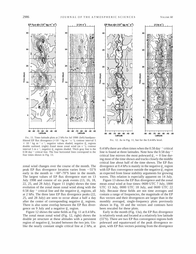
FIG. 11. Time–latitude plots at 2 hPa for Jul 1998: (left) bandpass-filtered EP flux divergence (31022 kg m21 s22), contour interval 53 1022 kg m21 s22, negative values shaded, negative y regionsqdouble outlined. (right) Zonal mean zonal wind (m s21), contourinterval 5 m s21, negative y regions shaded. Thick gray line is theq0.58 day21 critical line. The four horizontal lines correspond to thefour times shown in Fig. 13.
FIG. 12. As in Fig. 11, but for the 0.4-hPa level.
zonal wind changes over the course of the month. Thepeak EP flux divergence location varies from ;558Searly in the month to ;608–708S later in the month.The largest values of EP flux divergence start on 13July 1998 and consist of six peak events (13, 16, 18,22, 25, and 28 July). Figure 11 (right) shows the timeevolution of the zonal mean zonal wind along with the0.58 day21 critical line and the negative y regions, allqat 2 hPa. The three later EP flux divergence peaks (22,25, and 28 July) are seen to occur about a half a dayafter the center of corresponding negative y regions.qThere is also some overlap between the EP flux diver-gence on 9 July and a negative y region.q
Figure 12 shows the same fields as Fig. 11 at 0.4 hPa.The zonal mean zonal wind (Fig. 12, right) shows thedouble jet structure at these altitudes with a persistentregion of negative y located between the two jets. Un-qlike the nearly constant single critical line at 2 hPa, at
0.4 hPa there are often times when the 0.58 day21 criticalline is found at three latitudes. Note how the 0.58 day21
critical line mirrors the most poleward y 5 0 line dur-qing most of the time shown and tracks closely the middlecritical line about half of the time shown. The EP fluxdivergence at 0.4 hPa is mainly in the negative y regionqwith EP flux convergence outside the negative y regionqas expected from linear stability arguments for growingwaves. This relation is especially apparent on 14 July.
Figure 13 shows the EP flux divergence and the zonalmean zonal wind at four times: 0600 UTC 7 July, 1800UTC 13 July, 0000 UTC 18 July, and 0600 UTC 22July. Because these fields are not time averages andcontain a range of frequencies, the magnitude of the EPflux vectors and their divergences are larger than in themonthly averaged, single-frequency plots previouslyshown in Fig. 10 and the vectors and contours havebeen rescaled for these plots.
Early in the month (Fig. 13a), the EP flux divergenceis relatively weak and located at a relatively low latitude(558S). There are two EP flux convergence regions bothpoleward and equatorward of the peak divergence re-gion, with EP flux vectors pointing from the divergence

15 DECEMBER 2003 2987C O Y E T A L .
FIG. 13. Plots of (a), (c), (e), (g) EP flux divergence (contour interval 2.5 3 1022 kgm21 s22, negative values are shaded) and (b), (d), (f), (h) zonal mean zonal wind (contourinterval 10 m s21) at four times during Jul 1998. Eliassen–Palm flux vectors are scaled tobe 40% smaller than in Fig. 10 to aid readability. The heavy line on the right is the criticalline for a 1.72-day period wave-2 mode. Negative y regions are shaded on the right, andq
y 5 0 are double lines on the left.q
region into the convergence regions. These vectors cor-respond to both equatorward and poleward momentumfluxes at this time. This pattern of EP flux divergencewill tend to accelerate the winds between the split jet(Fig. 13b) and decelerate both jets, reducing the am-plitude of the negative y region as expected for unstableqwaves. The EP flux divergence at this time is somewhatcorrelated with the negative y region located betweenqthe split jet.
By 13 July, the EP flux divergence (Fig. 13c) is muchstronger and the peaks are displaced farther poleward(658S). While the EP flux divergence peaks below thenegative y region, there is still an EP flux divergenceqregion above 1 hPa that is well correlated with the neg-ative y region. There are two EP flux convergence re-qgions at this time: one above and poleward of the maindivergence peak, and one below the EP flux divergenceregion. The EP flux vectors are mainly poleward at this

2988 VOLUME 60J O U R N A L O F T H E A T M O S P H E R I C S C I E N C E S
FIG. 14. Longitude–time plot of POAM ozone (ppmv) at an averagelatitude of 688S and 2 hPa for Jul 1998. Contour interval is 0.5 ppmv.Lower ozone values are shaded.
time (equatorward momentum fluxes) except down near10 hPa where the EP flux vectors head toward the criticalline (Fig. 13d).
An even more poleward EP flux divergence peak isfound on 18 July (Fig. 13e), and it is clearly associatedwith a high-latitude negative y region. The polewardqjet is very weak at this time (Fig. 13f) and most of theEP flux vectors equatorward of 708S point equatorward(poleward momentum flux). The EP flux convergenceregion completely encircles the divergence region withespecially strong convergence above and below the di-vergence region.
Just 4 days later (about one rotational period) the EPflux divergence peak (Fig. 13g) is more equatorward(588S), and there are large regions of both poleward andequatorward EP flux vectors. The EP flux divergenceis well correlated with a negative y region, and theqdouble jet structure has returned (Fig. 13h). The EP fluxconvergence region wraps almost completely around thedivergence region.
These plots show that the positions of the EP fluxdivergence and negative y regions vary over the courseqof the month. In general the strong EP flux divergenceregions are closely associated with a negative y region;qhowever, the EP flux divergence regions are often strongoutside the negative y region. Thus the complete cor-qrelation between the two fields expected from lineartheory for growing waves [as discussed with Eq. (2)]does not occur, implying that the waves are either de-caying or influence by frictional, diabatic, nonlinear, orageostrophic effects in some regions.
4. POAM ozone data
This section presents the Polar Ozone and AerosolMeasurement (POAM) ozone data (Lucke et al. 1999)that observationally validates key features of the 4-daywave as seen in the DAO ozone assimilation. DuringJuly 1998 the POAM ozone observations were confinedbetween about 658–708S and therefore will be treatedas being at a constant latitude. There are ;14 ozoneprofiles taken each day. This does not give much res-olution for a longitude time plot; nevertheless, Fig. 14shows one attempt to interpolate the longitude–timePOAM observations at 2 hPa to a regular grid suitablefor contouring the high-frequency waves. Comparingwith the assimilation ozone (Fig. 1b), the POAM ob-servations show a similar time mean wave-1 structureand propagating wave-2 feature. The amplitude of thewave-2 signal in the POAM ozone is nearly the sameas in the DAO ozone assimilation (the contour intervalis doubled in Fig. 14), although there is an offset toslightly higher overall values of ozone in the POAMobservations. Note that lower resolution, combined withinterpolation, results in smoother contours in the POAMlongitude–time figure than in the corresponding DAOozone figure.
Figure 15 provides more quantitative evidence of the
high-frequency wave in the POAM observations usingan analysis method similar to that of Prata (1984). Here,the POAM observations at each level are taken as a timeseries for the month and a Fourier transform is per-formed on the month-long time series (431 points ateach level for the month of July 1998). This methoddoes not separate out the wavenumber dependence;however, stationary waves 1 and 2 would correspondto 1 and 2 day21 frequencies, respectively (as the earthrotates under the satellite), and 4-day rotational period;eastward-propagating waves 1 and 2 would correspondto 1.25 and 2.5 day21 frequencies, respectively (by add-ing the frequency of the wave motion to the correspond-ing frequency associated with the earth’s rotation). Theresults are plotted in two frequency ranges (Figs. 15aand 15b) to aid in making comparisons with Figs. 6band 6d. Figures 15a and 15b can be interpreted as wave-1 and wave-2 plots, though this interpretation of thePOAM observations is not unique.
Spectral analysis of the POAM time series reveals anoscillation near 2 hPa with a frequency of 2.58 days21
(Fig. 15b). A stationary wave 2 would yield a peak of2 days21 and an eastward-propagating wave 2 would
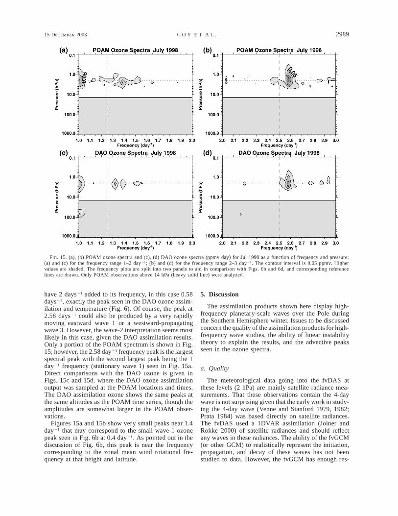
15 DECEMBER 2003 2989C O Y E T A L .
FIG. 15. (a), (b) POAM ozone spectra and (c), (d) DAO ozone spectra (ppmv day) for Jul 1998 as a function of frequency and pressure:(a) and (c) for the frequency range 1–2 day21; (b) and (d) for the frequency range 2–3 day21. The contour interval is 0.05 ppmv. Highervalues are shaded. The frequency plots are split into two panels to aid in comparison with Figs. 6b and 6d, and corresponding referencelines are drawn. Only POAM observations above 14 hPa (heavy solid line) were analyzed.
have 2 days21 added to its frequency, in this case 0.58days21, exactly the peak seen in the DAO ozone assim-ilation and temperature (Fig. 6). Of course, the peak at2.58 days21 could also be produced by a very rapidlymoving eastward wave 1 or a westward-propagatingwave 3. However, the wave-2 interpretation seems mostlikely in this case, given the DAO assimilation results.Only a portion of the POAM spectrum is shown in Fig.15; however, the 2.58 day21 frequency peak is the largestspectral peak with the second largest peak being the 1day21 frequency (stationary wave 1) seen in Fig. 15a.Direct comparisons with the DAO ozone is given inFigs. 15c and 15d, where the DAO ozone assimilationoutput was sampled at the POAM locations and times.The DAO assimilation ozone shows the same peaks atthe same altitudes as the POAM time series, though theamplitudes are somewhat larger in the POAM obser-vations.
Figures 15a and 15b show very small peaks near 1.4day21 that may correspond to the small wave-1 ozonepeak seen in Fig. 6b at 0.4 day21. As pointed out in thediscussion of Fig. 6b, this peak is near the frequencycorresponding to the zonal mean wind rotational fre-quency at that height and latitude.
5. Discussion
The assimilation products shown here display high-frequency planetary-scale waves over the Pole duringthe Southern Hemisphere winter. Issues to be discussedconcern the quality of the assimilation products for high-frequency wave studies, the ability of linear instabilitytheory to explain the results, and the advective peaksseen in the ozone spectra.
a. Quality
The meteorological data going into the fvDAS atthese levels (2 hPa) are mainly satellite radiance mea-surements. That these observations contain the 4-daywave is not surprising given that the early work in study-ing the 4-day wave (Venne and Stanford 1979, 1982;Prata 1984) was based directly on satellite radiances.The fvDAS used a 1DVAR assimilation (Joiner andRokke 2000) of satellite radiances and should reflectany waves in these radiances. The ability of the fvGCM(or other GCM) to realistically represent the initiation,propagation, and decay of these waves has not beenstudied to data. However, the fvGCM has enough res-

2990 VOLUME 60J O U R N A L O F T H E A T M O S P H E R I C S C I E N C E S
olution to assimilate the observations without the lossof information, and the appropriate dynamics and phys-ics to produce the 6-hourly forecasts of the observedwave structure for the next assimilation cycle. The in-dependent POAM observations indicate that the ozoneassimilation component, and therefore the advectingwinds, are being well handled by the data assimilationsystem.
The top level of the analysis may be too low to com-pletely characterize the waves. As mentioned in the in-troduction, the top analysis level is 0.4 hPa with thehighest pressure level output being slightly above it at0.2 hPa. The negative y region and the wave-2 criticalqlevel extend above this altitude. It would be more sat-isfying if the entire regions of unstable and high zonalwind speeds were captured. The fvGCM does extend to0.01 hPa so the whole region of instability may indeedbe contained by the fvDAS.
The ozone data assimilation system was run withoutchemistry at this time, relying on observations to correctfor photochemical modifications. This may lead to somebiases in the mean values and wave amplitudes in theozone assimilation; however, the basic patterns shouldbe captured via advection by the fvGCM coupled withthe ozone observations. Here, the 4-day wave signal inthe DAO assimilated ozone agreed well with contem-poraneous POAM ozone observations, providing somevalidation of the O3DAS.
Bandpassed-filtered fields were used here because the2-day wave signal was well defined and persistentthroughout July 1998. Generally the bandpassed-filteredfields closely followed the full wave pattern (by com-parison of corresponding maps, not shown); however,there were some specific times (mainly at the end ofthe month) when the maps based on bandpassed-filteredtemperatures did not closely resemble the maps basedon the full temperature field. At these times enhancedwave-1 and wave-3 components were also present, andthus, more spectral components or a non-Fourier ap-proach may give further insight into the dynamical sit-uation at these times.
The key to this study was the availability of dataassimilation products every 6 h. Such time resolutionresolves these fast-propagating and fast-changing wavesand thus permits a detailed study of their properties andevolution.
b. Instability theory
This study examined both the monthly averaged andinstantaneous EP flux vectors, EP flux divergences, andnegative y regions. The instantaneous fields can beqexpected to give the best agreement with the developingwave structure predicted by linear instability theory.
In linear instability theory, a negative y region isqcorrelated with a region of EP flux divergence. Hart-mann (1983) found exact correlation in his barotropicmodel. In their baroclinic model Manney and Randel
(1993) also found EP flux divergence and negative yqregions were very closely correlated. In this study, wefound that regions of EP flux divergence were not sotightly correlated with negative y regions. However,qthe instantaneous EP flux divergences were all closelyassociated with a negative y region. Looking at allqtimes during the month (not shown) reveals that thenegative y region often quickly disappears (within 6–q12 h) in the vicinity of a growing EP flux divergence.The negative y region is never completely eliminated,qbut rather tends to shift to a different latitude or height.
Along with instability, the wave structure seems toshow wave propagation away from the source regiontoward convergence at a critical level. This can be seenin the time-averaged plot (Fig. 10a), where the EP fluxvectors converge on the critical line at about 20 hPa.By contrast, EP flux vectors from a linear model shownin Manney and Randel (1993) are only large close tothe negative y region.q
Figure 2d shows how zonally asymmetric the negativepotential vorticity regions can be. This suggests that (inthis example at least) formulating the problem in termsof waves growing on a zonally symmetric unstable statemay only be a first step in understanding the origin andevolution of the waves. All of the zonally averaged EPflux divergence regions shown here overlap with neg-ative potential vorticity regions at some longitude (notshown). Additional consideration of the instability ofnonzonally symmetric flows (Manney et al. 1989) or amore three-dimensional modeling approach may beneeded.
Overall, our study supports earlier linear instabilitymodels that associate regions of potential vorticity in-stability as the source of the waves. The waves prop-agate (where y is positive) more slowly than the meanqwind in agreement with Rossby wave theory. In addi-tion, the wave’s vertical scale decreases as the wavesapproach the critical line from above, as seen in Fig.9c where the phase of the geopotential height field be-gins to change rapidly, again in agreement with linearRossby wave theory. The frequency of the wave is de-termined by the frequency of the zonal mean wind ro-tation around a latitude circle (the heavy line in Fig. 5is for the 1.72-day period, 0.58 day21 frequency forwavenumber 2) at the y 5 0 line in the region betweenqthe double jet.
c. Advective ozone peak
While the temperature spectra peak at frequencies thatimply phase speeds slower than the zonal mean zonalwind, the ozone spectra show a tendency for additionalpeaks at frequencies that imply phase speeds that arefaster than the zonal mean zonal wind speed (Fig. 7).This may imply that the wave-induced temperature re-sponse is more dynamically controlled than the ozoneresponse. Chemistry or diabatic processes may act tocreate ozone gradients along PV contours allowing the

15 DECEMBER 2003 2991C O Y E T A L .
wave-induced ozone response to have a passive advec-tion signal as well. While no signals like this were seenin the Manney et al. (1998) study of long-lived watervapor and methane, a large fast-moving ozone peak wasseen in the spectra presented in Allen et al. (1997). Theresults here should be interpreted with some caution asthese advective peaks were not identified prior to thespectral analysis and may be an artifact of the assimi-lation process or spectral analysis.
6. Conclusions
This paper has focused on a month (July 1998) whenthe wave-2 component of the 4-day wave was well de-fined and persistent. The availability of 6-hourly outputfrom the fvDAS has allowed the first detailed globalexamination of this fast-moving wave feature. In ad-dition, a companion ozone assimilation allowed iden-tification of the high-frequency wave in the assimilatedozone field.
This wave-2 component (1.7-day period) is generallyconsistent with past observational studies and linear in-stability models. Enhanced EP flux divergence is closelyassociated with negative y regions with the wave am-qplitude mainly confined by the critical line to phasespeeds westward with respect to the mean flow.
Wave 2 also appears prominently in the DAO ozoneassimilation, having an amplitude of about 0.5 ppmv or;15% of the total ozone mixing ratio at 2 hPa andcontaining ;50% of the total ozone variance at 708S.This ozone signal is supported by independent POAMozone mixing ratio observations. POAM ozone time se-ries at ;708S shows a spectral peak at 2.58 day21 thatis consistent with the assimilation results. The amplitudeof the 2.58 day21 signal in POAM (Fig. 14) is veryclose to the amplitude of the wave 2, 0.58 day21 signalin the DAO ozone assimilation (Figs. 6d and 15d) andboth show the ozone spectra at those frequencies peak-ing near 2 hPa.
The region of reversed temperature gradient was not-ed in Fig. 5b. This temperature pattern is needed tosupport the mean wind structure that, in turn, is neededfor the 4-day waves to grow. How much, if any, of thismean structure might be caused by the 4-day wave act-ing on the mean state is still an open question.
The ability of the geopotential height alone to gen-erate the complex EP flux patterns seen in the assimi-lation-produced wind and temperature fields was illus-trated in Figs. 10a and 10b. This implies that, if thegeopotential heights are accurate enough, studies ofcomplex EP flux patterns are possible using only geo-potential height observations.
While the wave can appear fairly steady over thecourse of a month, the EP flux divergence pattern canvary significantly over the course of a wave period asshown here for the wave-2 component, and in Randeland Lait (1991) and Lawrence and Randel (1996) forthe wave-1 component. This probably indicates that
more detailed examination of these waves and their de-velopment may be possible using instantaneous PVmaps. This leaves open future studies based on assim-ilation products to further understand the origin anddevelopment of high-frequency polar waves.
Acknowledgments. We would like to thank StephenEckermann for reviewing an early draft of this work.We would also like to thank the POAM team for guid-ance in using the POAM ozone measurements. The workwas supported in part by the Office of Naval Research.The development and use of the fvDAS was supportedby NASA, through their Earth Observation System re-search program.
REFERENCES
Allen, D. R., J. L. Stanford, L. S. Elson, E. F. Fishbein, L. Froidevaux,and J. W. Waters, 1997: The 4-day wave as observed from theUpper Atmosphere Research Satellite Microwave Limb Sounder.J. Atmos. Sci., 54, 420–434.
Andrews, D. G., J. R. Holton, and C. B. Leovy, 1987: Middle At-mosphere Dynamics. Academic Press, 489 pp.
Cohn, S. E., A. DaSilva, J. Guo, M. Sienkiewicz, and D. Lamich,1998: Assessing the effects of data selection with the DAO phys-ical-space statistical analysis system. Mon. Wea. Rev., 126,2913–2926.
Douglass, A. R., M. R. Schoeberl, R. B. Rood, and S. Pawson, 2003:Evaluation of transport in the lower tropical stratosphere in aglobal chemistry and transport model. J. Geophys. Res., 108,4259, doi:10.1029/2002JD002696.
Hartmann, D. L., 1983: Barotropic instability of the polar night jetstream. J. Atmos. Sci., 40, 817–835.
Holton, J. R., 1992: An Introduction to Dynamic Meteorology. Ac-ademic Press, 511 pp.
Joiner, J., and L. Rokke, 2000: Variational cloud clearing with TOVSdata. Quart. J. Roy. Meteor. Soc., 126, 725–748.
Kiehl, J. T., J. J. Hack, G. B. Bonan, B. A. Boville, D. L. Williamson,and P. J. Rasch, 1988: The National Center for AtmosphericResearch Community Climate Model: CCM3. J. Climate, 11,1131–1149.
Lait, L. R., and J. L. Stanford, 1988: Fast, long-lived features in thepolar stratosphere. J. Atmos. Sci., 45, 3800–3809.
Lawrence, B. N., and W. J. Randel, 1996: Variability in the meso-sphere observed by the Nimbus 6 PMR. J. Geophys. Res., 101,23 475–23 489.
——, G. J. Fraser, R. A. Vincent, and A. Philips, 1995: The 4-daywave in the Antarctic mesosphere. J. Geophys. Res., 100, 18 899–18 908.
Lin, S. J., 1997: A finite-volume integration method for computingpressure gradient force in general vertical coordinates. Quart. J.Roy. Meteor. Soc., 123, 1749–1762.
——, and R. B. Rood, 1996: Multidimensional flux-form semi-La-grangian transport schemes. Mon. Wea. Rev., 124, 2046–2070.
——, and ——, 1997: An explicit flux-form semi-Lagrangian shal-low-water model on the sphere. Quart. J. Roy. Meteor. Soc.,123, 2477–2498.
Lucke, R. L., and Coauthors, 1999: The Polar Ozone and AerosolMeasurement (POAM) III instrument and early validation re-sults. J. Geophys. Res., 104, 18 785–18 799.
Manney, G. L., 1991: The stratospheric 4-day wave in NMC data. J.Atmos. Sci., 48, 1798–1811.
——, and W. J. Randel, 1993: Instability at the winter stratopause:A mechanism for the 4-day wave. J. Atmos. Sci., 50, 3928–3938.
——, T. R. Nathan, and J. L. Stanford, 1988: Barotropic stability ofrealistic stratospheric jets. J. Atmos. Sci., 45, 2545–2555.

2992 VOLUME 60J O U R N A L O F T H E A T M O S P H E R I C S C I E N C E S
——, ——, and ——, 1989: Barotropic instability of basic stateswith a realistic jet and a wave. J. Atmos. Sci., 46, 1250–1273.
——, Y. J. Orsolini, H. C. Pumphrey, and A. E. Roche, 1998: The4-day wave and transport of UARS tracers in the austral polarvortex. J. Atmos. Sci., 55, 3456–3470.
Prata, A. J., 1984: The 4-day wave. J. Atmos. Sci., 41, 150–155.Randel, W. J., and L. R. Lait, 1991: Dynamics of the 4-day wave in
the Southern Hemisphere polar stratosphere. J. Atmos. Sci., 48,2496–2508.
Schoeberl, M. R., A. R. Douglass, Z. X. Zhu, and S. Pawson, 2003:
A comparison of the lower stratospheric age spectra derived froma general circulation model and two data assimilation systems.J. Geophys. Res., 108, 4113, doi:10.1029/2002JD002652.
Stajner, I., L. P. Riishojgaard, and R. B. Rood, 2001: The GEOSozone data assimilation system: Specification of error statistics.Quart. J. Roy. Meteor. Soc., 127, 1069–1094.
Venne, D. E., and J. L. Stanford, 1979: Observations of a 4-daytemperature wave in the polar winter stratosphere. J. Atmos. Sci.,36, 2016–2019.
——, and ——, 1982: An observational study of high-latitude strato-spheric planetary waves in winter. J. Atmos. Sci., 39, 1026–1034.