high speed solution of spacecraft trajectory problems

James R. Scott Glenn Research Center, Cleveland, Ohio

Michael C. MartiniAnalex Corporation, Cleveland, Ohio

High Speed Solution of Spacecraft Trajectory Problems Using Taylor Series Integration

NASA/TM—2008-215439

August 2008

AIAA–2008–6957

NASA STI Program . . . in Profi le

Since its founding, NASA has been dedicated to the advancement of aeronautics and space science. The NASA Scientifi c and Technical Information (STI) program plays a key part in helping NASA maintain this important role.

The NASA STI Program operates under the auspices of the Agency Chief Information Offi cer. It collects, organizes, provides for archiving, and disseminates NASA’s STI. The NASA STI program provides access to the NASA Aeronautics and Space Database and its public interface, the NASA Technical Reports Server, thus providing one of the largest collections of aeronautical and space science STI in the world. Results are published in both non-NASA channels and by NASA in the NASA STI Report Series, which includes the following report types: • TECHNICAL PUBLICATION. Reports of

completed research or a major signifi cant phase of research that present the results of NASA programs and include extensive data or theoretical analysis. Includes compilations of signifi cant scientifi c and technical data and information deemed to be of continuing reference value. NASA counterpart of peer-reviewed formal professional papers but has less stringent limitations on manuscript length and extent of graphic presentations.

• TECHNICAL MEMORANDUM. Scientifi c

and technical fi ndings that are preliminary or of specialized interest, e.g., quick release reports, working papers, and bibliographies that contain minimal annotation. Does not contain extensive analysis.

• CONTRACTOR REPORT. Scientifi c and

technical fi ndings by NASA-sponsored contractors and grantees.

• CONFERENCE PUBLICATION. Collected

papers from scientifi c and technical conferences, symposia, seminars, or other meetings sponsored or cosponsored by NASA.

• SPECIAL PUBLICATION. Scientifi c,

technical, or historical information from NASA programs, projects, and missions, often concerned with subjects having substantial public interest.

• TECHNICAL TRANSLATION. English-

language translations of foreign scientifi c and technical material pertinent to NASA’s mission.

Specialized services also include creating custom thesauri, building customized databases, organizing and publishing research results.

For more information about the NASA STI program, see the following:

• Access the NASA STI program home page at http://www.sti.nasa.gov

• E-mail your question via the Internet to help@

sti.nasa.gov • Fax your question to the NASA STI Help Desk

at 301–621–0134 • Telephone the NASA STI Help Desk at 301–621–0390 • Write to:

NASA Center for AeroSpace Information (CASI) 7115 Standard Drive Hanover, MD 21076–1320

James R. Scott Glenn Research Center, Cleveland, Ohio

Michael C. MartiniAnalex Corporation, Cleveland, Ohio


NASA/TM—2008-215439

August 2008

AIAA–2008–6957

National Aeronautics andSpace Administration

Glenn Research CenterCleveland, Ohio 44135

Prepared for theAstrodynamics Specialist Conference and Exhibitsponsored by the American Institute of Aeronautics and Astronautics and the American Astronautical SocietyHonolulu, Hawaii, August 18–21, 2008

Acknowledgments

The authors would like to thank Glen Horvat and Kurt Hack for their support of this work.

Available from

NASA Center for Aerospace Information7115 Standard DriveHanover, MD 21076–1320

National Technical Information Service5285 Port Royal RoadSpringfi eld, VA 22161

Available electronically at http://gltrs.grc.nasa.gov

Level of Review: This material has been technically reviewed by technical management.

This report is a preprint of a paper intended for presentation at a conference. Because changes may be made before formal publication, this preprint is made available

with the understanding that it will not be cited or reproduced without the permission of the author.


Taylor series integration is implemented in a spacecraft trajectory analysis code – the Spacecraft N-body Analysis Program (SNAP) – and compared with the code’s existing eighth-order Runge-Kutta Fehlberg time integration scheme. Nine trajectory problems, including near Earth, lunar, Mars and Europa missions, are analyzed. Head-to-head comparison at five different error tolerances shows that, on average, Taylor series is faster than Runge-Kutta Fehlberg by a factor of 15.8. Results further show that Taylor series has superior convergence properties. Taylor series integration proves that it can provide rapid, highly accurate solutions to spacecraft trajectory problems.

Nomenclature

1x = x component of spacecraft position relative to inertial frame centered at the central body

2x = y component of spacecraft position relative to inertial frame centered at the central body

3x = z component of spacecraft position relative to inertial frame centered at the central body

4x = x component of spacecraft velocity relative to inertial frame centered at the central body

5x = y component of spacecraft velocity relative to inertial frame centered at the central body

6x = z component of spacecraft velocity relative to inertial frame centered at the central body

7x = spacecraft mass

X = ),,,,,,( 7654321 xxxxxxx = spacecraft state vector

xr

= ),,( 321 xxx = spacecraft position vector

vr

= ),,(),,( 321654 vvvxxx = = spacecraft velocity vector t = time ′ = d/dt = derivative with respect to time ⋅ = d/dt = derivative with respect to time m& = mass flow rate T = thrust magnitude

1a = x component of spacecraft acceleration relative to inertial frame centered at the central body

2a = y component of spacecraft acceleration relative to inertial frame centered at the central body

3a = z component of spacecraft acceleration relative to inertial frame centered at the central body

James R. Scott National Aeronautics and Space Administration

Glenn Research Center Cleveland, Ohio 44135

Michael C. Martini Analex Corporation

Cleveland, Ohio 44135

NASA/TM—2008-215439 1

ar

= ),,( 321 aaa = acceleration vector

jxr

= position vector of the jth other body relative to the central body

G = gravitational constant M = body mass h = step size ! = local error tolerance ! = step multiplication factor

I. Introduction he advantages of Taylor series integration in solving ordinary differential equations have been known for some time 1-25. Foremost among these is the ability to maintain very high computational efficiency while achieving

high accuracy. In fact, comparisons with other methods have shown that Taylor series integration can be faster by a factor of twenty or more 20. The success of the method depends on recasting the governing differential system into a canonical form whereby system derivatives can be obtained to arbitrary order through recursion. This obviates the need to directly calculate derivatives, and makes it possible to obtain derivative information cheaply. The system variables can thus be expanded in a highly accurate series at each time level at minimal cost. It turns out that most differential systems can be recast into the required canonical form in a straightforward manner. This has led a number of authors to develop general purpose software which can recast an arbitrary system into canonical form and solve the resulting equations automatically 10, 11, 15-18, 22-24. Taylor series integration can thus be used as both a general purpose solver and also for specific applications. The focus here is on calculating spacecraft trajectories. Previous work using Taylor series to calculate trajectories includes that in Refs. 21 and 22. Unlike Refs. 21 and 22, which used an automated Taylor series package 16,22 to propagate trajectories in Earth orbit, the present work focuses on using Taylor series integration in an existing trajectory analysis code, SNAP (Spacecraft N-body Analysis Program) 26. Developed at NASA’s Glenn Research Center, SNAP is a high fidelity trajectory propagation program that can propagate the trajectory of a spacecraft about virtually any body in the solar system. The equations of motion include the effects of central body gravitation with N x N harmonics, other body gravitation with N x N harmonics, solar radiation pressure, atmospheric drag (for Earth orbits) and spacecraft thrusting (including shadowing). The equations are solved using an eighth-order Runge-Kutta Fehlberg (RKF) 27 single step method with variable step size control. The purpose of this paper is to demonstrate the use of Taylor series (TS) integration in a high fidelity trajectory analysis code, SNAP, and to provide a detailed comparison of TS performance to eighth-order RKF 27. Section II presents the equations of motion, Section III describes the TS formulation and Section IV discusses the numerical implementation. Section V compares TS and RKF on a representative set of spacecraft trajectory problems, including near Earth, lunar, Mars and Europa missions. It is shown that TS is faster than RKF by an average factor of 15.8, while simultaneously improving accuracy.

II. Equations of Motion

Let ),,,,,,( 7654321 xxxxxxxX = denote the spacecraft state vector, where xxxxr

=),,( 321 is the spacecraft position in Cartesian coordinates relative to an inertial frame centered at the central body,

vxxxr

=),,( 654 is the spacecraft velocity relative to an inertial frame centered at the central body, and 7x is the

spacecraft mass. The equations of motion are

63

52

41

xx

xx

xx

=!

=!

=!

(1)

T

NASA/TM—2008-215439 2

)(

),,,,,,,(

),,,,,,,(

),,,,,,,(

7

765432136

765432125

765432114

tmx

txxxxxxxax

txxxxxxxax

txxxxxxxax

&!="

="

="

="

where

ia is the acceleration in the ith coordinate direction and m& is the mass flow rate. The acceleration is a

function of the forces acting on the spacecraft. Forces included in SNAP are central body, other body, thrust, atmospheric drag (for low Earth orbits), solar radiation pressure, oblateness effects of Earth, and oblateness effects of other bodies, so that

oboobesrpdthobcb aaaaaaaarrrrrrrr

++++++= (2) This paper considers only the first four acceleration terms, which are given below.

3

2

3

2

3

2

2

2

1

, :

)(x

xMG

xxx

xMGa

i

cb

i

cbicb r!=

++

!= (3)

where G is the gravitational constant,

cbM is the central body mass, i = 1,2,3 denotes the coordinate direction, and

the spacecraft mass is much less than the central body mass.

!!!

"

#

$$$

%

&+

'

''=( 3

,

3

,

,

j

ji

j

jii

j

jiob

x

x

xx

xxMGa

rrr (4)

where j denotes the jth body and ( )21

2

,3

2

,2

2

,1:

jjjjxxxx ++=

r.

7

,

1

xv

vTa

i

ith r= (5)

where T is the constant thrust magnitude and the thrust direction is parallel to the velocity vector.

( ) ( )[ ] ( )7224

2

1

2

6

2

125

2

22411, / xxcxxxcxxcxcad

++!++= (6)

( ) ( )[ ] ( )7125

2

1

2

6

2

125

2

22412, / xxcxxxcxxcxcad

!+!++= (7)

( ) ( )[ ]76

2

1

2

6

2

125

2

22413, / xxxxcxxcxcad

+!++= (8)

where )()(2

11 densitycatmospheriareaspacecraftCc D !!"= ,

2c = rotation rate of Earth and

DC is the

drag coefficient.

NASA/TM—2008-215439 3

III. Taylor Series Formulation

Let the state vector X have initial condition 0X . Within the radius of convergence, the system variables

)(txn

can be expanded in a Taylor series,

7,...,1,)(!

)()( 0

0

0

)(

=!="#

=

nttk

txtx

k

k

k

n

n (9)

where the derivatives )(k

nx are obtained by successively differentiating the right hand side of Eqs. (1). This can be

efficiently accomplished using recurrence relations, as follows. Consider only the central body acceleration term, so that

(10)

Introduce

8x and

9x ,

2

3

2

2

2

18xxxx ++= (11)

2/3

89xx = (12)

Eqs. (10) become

41xx =!

52xx =!

63xx =!

9

1

4

x

xMGx

cb!=" (13)

9

2

5

x

xMGx

cb!="

0

)(

)(

)(

7

2

3

2

3

2

2

2

1

36

2

3

2

3

2

2

2

1

25

2

3

2

3

2

2

2

1

14

63

52

41

=!

++

"=!

++

"=!

++

"=!

=!

=!

=!

x

xxx

xMGx

xxx

xMGx

xxx

xMGx

xx

xx

xx

cb

cb

cb

NASA/TM—2008-215439 4

9

3

6

x

xMGx

cb!="

07=!x

and two auxiliary equations are added to the system:

6352418222 xxxxxxx ++=! (14)

8

89

9

2

3

x

xxx

!=! (15)

The right hand side of the new system, Eqs. (13) – (15), can now be differentiated using recurrence relations for products and quotients.

For a function )()()( tgtftw = , the Leibnitz rule for differentiating products gives 16

!=

"=k

j

jkGjFkW0

)()()( (16)

where !

)(:)( 0

)(

k

twkW

k

= , !

)(:)( 0

)(

j

tfjF

j

= and )!(

)(:)( 0

)(

jk

tgjkG

jk

!=!

!

are reduced derivatives.

For a function )(

)()(

tg

tftw = , the recurrence relation for quotients gives 11

!"

#$%

&''= (

=

k

j

jkWjGkFg

kW1

)()()(1

)( (17)

where W, F and G are reduced derivatives as above. The recurrence relations are derived as follows. Let

9,...,1, =!= nxunn

(18)

Eqs. (13) – (15) become

41xu = (19)

52xu = (20)

63xu = (21)

9

1

4

x

xMGu

cb!= (22)

9

2

5

x

xMGu

cb!= (23)

NASA/TM—2008-215439 5

9

3

6

x

xMGu

cb!= (24)

07=u (25)

6352418222 xxxxxxu ++= (26)

8

89

9

2

3

x

uxu = (27)

Introduce auxiliary functions 9

1

4

x

xw = ,

9

2

5

x

xw = ,

9

3

6

x

xw = ,

411,8xxw = ,

522,8xxw = ,

633,8xxw = ,

and8

89

9

x

uxw = .

Using Eq. (18) one obtains

)()1( k

n

k

nxu =

! , 1!k (28) from which

)!1()!1(

)()1(

!=

!

!

k

x

k

uk

n

k

n , 1!k (29)

k

kUkXkXkkU

n

nnn

)1()()()1(

!="=!" , 1!k (30)

The recurrence relations are then, for all 1!k ,

k

kUkXkU

)1()()( 4

41

!== (31)

k

kUkXkU

)1()()( 5

52

!== (32)

k

kUkXkU

)1()()( 6

63

!== (33)

)()( 44 kWMGkU

cb!= (34)

)()( 55 kWMGkU

cb!= (35)

)()( 66 kWMGkU

cb!= (36)

NASA/TM—2008-215439 6

0)(7 =kU (37)

)(2)(2)(2)( 3,82,81,88 kWkWkWkU ++= (38)

)(2

3)( 99 kWkU = (39)

where

=!"

#$%

&''= (

=

k

j

jkWjXkXx

kW1

491

9

4 )()()(1

)( !"

#$%

&'

''

'(=

k

j

jkWj

jU

k

kU

x 1

491

9

)()1()1(1

(40)

!=

"=k

j

jkXjXkW0

411,8 )()()( jk

jkU

j

jUx

k

kU

k

kUx

k

j !

!!!+

!+

!= "

!

=

)1()1()1()1( 41

1

14

141 (41)

etc., and a similar expression can be derived for 9

W . The Taylor series coefficients are then

Kkk

kUkX

k

xn

n

k

n !!"

== 1,)1(

)(:!

)(

(42)

and the local series solution is

Kn

k

K

k

k

n

nTtt

k

txtx ,0

0

0

)(

)(!

)()( +!="

=

(43)

where )(kU

n is defined by Eqs. (31) – (39), )0(

nU is defined by Eqs. (19) – (27), K is the number of terms in the

series and Kn

T,

is the truncation error. The other acceleration terms can be handled similarly. Only other body acceleration, Eq. (4), requires special

consideration, due to the need for the motion of other bodies. This can generally be obtained from ephemeris files. However, integration by Taylor series requires derivatives not available from ephemeris files. It is thus necessary to integrate the other body motion as part of the governing differential system. This leads to a substantially larger system of equations, but fortunately can still be integrated efficiently.

Once the recurrence relations are derived for all acceleration terms and the state vector specified, Eqs. (42) – (43) are used to expand the system variables in a series from

0t to

1t , where the step size

011: tth != is

determined to meet the local error tolerance. From 1t , the variables are expanded in a new series to

2t , and so

forth. Thus, by a process of “analytic continuation,” one obtains a set of overlapping series solutions that cover the integration domain.

IV. Numerical Implementation Taylor series integration was implemented in SNAP by making some minor modifications to existing source

code and adding three additional subroutines - a driver routine which automatically introduces auxiliary variables, sets up initial conditions and integrates; a routine which calculates system reduced derivatives using recurrence

NASA/TM—2008-215439 7

relations for the following quotients and products: ,

n

m

x

x ,

nmxx ,

n

nm

x

xx !mmxx ! , ,

n

m

x

x!

l

nm

x

xx and

nmxx ! ; and a

routine which determines the step size and sums the series. The number of series terms is variable up to a maximum of 30, but remains constant throughout the integration. Positive and negative terms are summed separately to avoid cancellation of significant digits.

The step size can be determined from the standard formula 28

M

ehh

1

max

next !!"

#$$%

&=

'( (44)

where h denotes the current step, ! the local error tolerance, maxe the estimate of maximum truncation error, M

the order of the maximum truncation error estimate and 1<! the step multiplication factor. Eq. (44) is more or

less restrictive depending on ! and the truncation error estimate maxe . Generally,

maxe should not be calculated

from the next series term, due to the extra computation required and the fact that it is not a reliable error estimate 29. A conservative approach which takes advantage of the series terms already computed leads to

][ )()1(Max 1

max

K

n

K

nnhKXhKXe +!=

! (45)

where the expression in brackets is derived by subtracting the Taylor series solution of degree K - 2 from the solution of degree K and taking absolute values of individual terms. Eq. (45) can be viewed as a truncation error estimate for the series of degree K – 2 which is then applied to the more accurate series of degree K. An alternative to Eqs. (44) – (45) is to simply require h to be small enough that the system variables directly satisfy the absolute error tolerance requirement

!"+## K

n

K

nhKXhKX )()1( 1 (46)

for all n. Eq. (46) can be solved by fixed point iteration,

=+1lh !!

"

#

$$

%

&

+'' )()1(ln

1

1exp

KXhKXKnln

( (47)

The smallest h is chosen over all n, and multiplied by the step multiplication factor ! . This approach offers the advantage of directly calculating the step size without the need for a previous step, and guarantees that the error tolerance is met. Eq. (44), on the other hand, requires a previous step and will require a repeat step whenever

!>maxe . The step selection methods above performed very similarly in the current study. Both methods provided stable, accurate solutions and used approximately the same number of time steps in head-to-head calculations.

V. Results We compare RKF and TS performance on the trajectory problems in Table 1. All calculations were run on a Dell PowerEdge 2600 with two 3.066 GHz processors and four GB of RAM. Source code was compiled using the Absoft Fortran 90 compiler without optimization. SNAP was run with all intermediate print and stop options turned off. All TS calculations used a series with 20 terms and a variable step size determined by Eq. (47) with a step multiplication factor that ranged from 0.75 to 0.9.

NASA/TM—2008-215439 8

Table 1 Problem Title Description Central

Body Other Bodies

1 Satellite in low Earth orbit (LEO)

A 10,000 kg satellite orbits Earth for 10 days at an inclination of 28.45 degrees.

Earth Moon

2 Satellite in LEO with drag

A 10,000 kg satellite orbits Earth for 10 days with constant drag at an inclination of 28.45 degrees.

Earth Moon

3 Spacecraft spiraling out of Earth’s gravity well

A 10,000 kg spacecraft spirals out of Earth’s gravity well in a low thrust trajectory. Calculation stops when the semi-major axis of trajectory equals 40,000 km.

Earth Sun, Moon

4 Spacecraft from near Earth to lunar orbit

A 3580 kg spacecraft 400 km above Earth has been propelled with sufficient energy to reach the Moon. Spacecraft coasts to Moon, performs insertion burn, propagates to apolune, and performs final burn to achieve 500 km by 10,000 km polar lunar orbit with an argument of perilune equal to 90 degrees. See Fig. 1.

Moon Earth, Sun

5 Spacecraft in lunar orbit

Spacecraft with 2848.56 kg mass coasts for 10 days in 500 km by 10,000 km polar lunar orbit with an argument of perilune equal to 90 degrees. See Fig. 1.

Moon Earth, Sun

6 Spacecraft thrusting from near Earth to Mars coast

A 585 kg spacecraft near Earth thrusts for 38.45 days to achieve sufficient energy to coast to Mars. See Fig. 2.

Sun Earth, Moon, Venus, Mars, Jupiter barycenter, Saturn barycenter

7 Spacecraft coast to Mars flyby

A 555.66 kg spacecraft coasts to Mars flyby for 161.55 days. See Fig. 2.

Sun Earth, Moon, Venus, Mars, Jupiter barycenter, Saturn barycenter

8 Spacecraft thrusting tangentially out of Europa orbit

A 10,000 kg spacecraft in Europa orbit thrusts tangentially to spiral out until the semi-major axis equals 10,000 km.

Europa Jupiter, Sun, Ganymede, Io Callisto

9 Spacecraft coast near Europa

A 9800.49 kg spacecraft coasts for one day after spiraling out of Europa orbit.

Europa Jupiter, Sun, Ganymede, Io Callisto

Figure 1. Earth to Moon Trajectory Figure 2. Earth to Mars Flyby

NASA/TM—2008-215439 9

Each trajectory was integrated at five error tolerances from 1010

! to 1410

! . Tables 2 - 10 summarize the results. RKF results are shown on top and TS on bottom. Spacecraft positions are in kilometers and CPU ratio is RKF/TS. RKF and TS velocities agreed equally well as spacecraft position, but are omitted here for brevity.

Table 2 Results for Problem 1 Spacecraft Position at End of Calculation CPU CPU ! x y z (sec) ratio 1.E-10 -4505.4956174253 4460.8015923075 2416.2243468200 6.91 1.E-11 -4505.4976241104 4460.8000212437 2416.2234952381 9.10 1.E-12 -4505.4977855238 4460.7998948715 2416.2234267390 12.23 1.E-13 -4505.4977981582 4460.7998849798 2416.2234213773 16.05 1.E-14 -4505.4977991371 4460.7998842135 2416.2234209620 21.17 1.E-10 -4505.4893402433 4460.8066582279 2416.2273550484 0.20 34.6 1.E-11 -4505.4893401709 4460.8066582847 2416.2273550792 0.22 41.4 1.E-12 -4505.4893402598 4460.8066582151 2416.2273550415 0.25 48.9 1.E-13 -4505.4893403875 4460.8066581153 2416.2273549873 0.28 57.3 1.E-14 -4505.4893402869 4460.8066581940 2416.2273550300 0.31 68.3


Table 4 Results for Problem 3 Spacecraft Position at End of Calculation CPU CPU ! x y z (sec) ratio 1.E-10 21783.589218926 30426.566335107 14117.151742798 44.01 1.E-11 21783.168251826 30426.814392403 14117.266771932 58.17 1.E-12 21783.134612346 30426.834214343 14117.275963762 77.72 1.E-13 21783.131993250 30426.835757635 14117.276679417 102.06 1.E-14 21783.131799858 30426.835871591 14117.276732261 134.87 1.E-10 21783.126013948 30426.839470527 14117.277961164 2.29 19.2 1.E-11 21783.126025067 30426.839463974 14117.277958125 2.57 22.6 1.E-12 21783.126012532 30426.839471362 14117.277961551 2.88 27.0 1.E-13 21783.126009565 30426.839473099 14117.277962357 3.27 31.2 1.E-14 21783.126006877 30426.839474690 14117.277963095 3.69 36.6

NASA/TM—2008-215439 10

Table 5 Results for Problem 4 Spacecraft Position at End of Calculation CPU CPU ! x y z (sec) ratio 1.E-10 -178.63870529793 4876.3161604664 -10650.392195425 0.44 1.E-11 -178.63855098380 4876.3170369698 -10650.391796702 0.51 1.E-12 -178.63855046608 4876.3170506570 -10650.391790443 0.59 1.E-13 -178.63855601675 4876.3170085371 -10650.391809627 0.71 1.E-14 -178.63854695266 4876.3170607540 -10650.391785873 0.87 1.E-10 -178.71939471463 4876.1033547743 -10650.488272923 0.19 2.31 1.E-11 -178.71939481530 4876.1033542962 -10650.488273141 0.20 2.55 1.E-12 -178.71939478451 4876.1033544409 -10650.488273078 0.20 2.95 1.E-13 -178.71939478450 4876.1033544292 -10650.488273079 0.20 3.55 1.E-14 -178.71939478714 4876.1033544962 -10650.488273051 0.20 4.35

Table 6 Results for Problem 5 Spacecraft Position at End of Calculation CPU CPU ! x y z (sec) ratio 1.E-10 -215.32731201862 -1650.3697144277 1635.1626824928 1.99 1.E-11 -215.32794605537 -1650.3715299629 1635.1612149497 2.64 1.E-12 -215.32799474610 -1650.37166939046 1635.1611022567 3.49 1.E-13 -215.32799868206 -1650.3716806616 1635.1610931478 4.62 1.E-14 -215.32799901817 -1650.3716816241 1635.1610923701 6.15 1.E-10 -215.32849813488 -1650.3731189359 1635.1600219626 0.32 6.22 1.E-11 -215.32849812774 -1650.3731189154 1635.1600219790 0.35 7.54 1.E-12 -215.32849812980 -1650.3731189214 1635.1600219744 0.40 8.73 1.E-13 -215.32849813332 -1650.3731189310 1635.1600219653 0.44 10.5 1.E-14 -215.32849813453 -1650.3731189349 1635.1600219635 0.49 12.6

Table 7 Results for Problem 6 Spacecraft Position at End of Calculation CPU CPU ! x y z (sec) ratio 1.E-10 21572817.105605 -139377155.25969 -62943596.519662 0.14 1.E-11 21572817.105556 -139377155.25962 -62943596.519125 0.15 1.E-12 21572817.105508 -139377155.25961 -62943596.519004 0.21 1.E-13 21572817.105509 -139377155.25960 -62943596.518999 0.25 1.E-14 21572817.105496 -139377155.25961 -62943596.518987 0.34 1.E-10 21572816.904607 -139377156.15407 -62943596.9802248 0.11 1.27 1.E-11 21572816.904606 -139377156.15407 -62943596.9802247 0.12 1.25 1.E-12 21572816.904607 -139377156.15407 62943596.9802248 0.14 1.50 1.E-13 21572816.904607 -139377156.15407 -62943596.9802248 0.16 1.56 1.E-14 21572816.904607 -139377156.15407 -62943596.9802247 0.17 2.00

NASA/TM—2008-215439 11

Table 11 summarizes the CPU ratios. TS is faster than RKF by more than an order of magnitude in 18 of 45 cases. The average speedup is 15.8. For the interplanetary trajectory problems (4-9) the average speedup is 4.53. The gain here is smaller due to the additional equations that TS must solve to account for other body motion. As noted previously, TS must integrate other body motion as part of the differential system, whereas RKF obtains other body motion from ephemeris files. This difference in the integration methods explains the small differences in spacecraft positions observed in Tables 2-10.

Table 8 Results for Problem 7 Spacecraft Position at End of Calculation CPU CPU ! x y z (sec) ratio 1.E-10 174298859.53574 117412103.45296 49149031.016983 0.14 1.E-11 174298859.53061 117412103.45425 49149031.017954 0.15 1.E-12 174298859.53010 117412103.45436 49149031.018040 0.17 1.E-13 174298859.53005 117412103.45437 49149031.018048 0.18 1.E-14 174298859.53003 117412103.45437 49149031.018052 0.23 1.E-10 174298891.93452 117412111.58059 49149027.497160 0.11 1.27 1.E-11 174298891.93452 117412111.58059 49149027.497159 0.13 1.15 1.E-12 174298891.93452 117412111.58059 49149027.497160 0.15 1.13 1.E-13 174298891.93453 117412111.58059 49149027.497159 0.17 1.06 1.E-14 174298891.93453 117412111.58059 49149027.497159 0.17 1.35

Table 9 Results for Problem 8 Spacecraft Position at End of Calculation CPU CPU ! x y z (sec) ratio 1.E-10 7528.3536043710 1375.7425889427 -383.13557482604 0.79 1.E-11 7528.3536031572 1375.7425956652 -383.13557244841 1.00 1.E-12 7528.3536030460 1375.7425962755 -383.13557223246 1.33 1.E-13 7528.3536030359 1375.7425963294 -383.13557221337 1.74 1.E-14 7528.3536030345 1375.7425963361 -383.13557221099 2.25 1.E-10 7528.7471022132 1375.7729665868 -383.16004903160 0.14 5.64 1.E-11 7528.7471022129 1375.7729665694 -383.16004903738 0.15 6.67 1.E-12 7528.7471022110 1375.7729665782 -383.16004903433 0.16 8.31 1.E-13 7528.7471022134 1375.7729665759 -383.16004903524 0.18 9.67 1.E-14 7528.7471022136 1375.7729665815 -383.16004903345 0.21 10.7


NASA/TM—2008-215439 12

Another important property to consider is convergence. Tables 12 - 20 present the number of converged digits obtained for each spacecraft coordinate at each error tolerance, where the 14

10!

=" case was used as the fully converged solution. RKF results are on top and TS on bottom. TS has more converged digits than RKF in 103 out of 108 cases, while RKF has more converged digits in one case. On average, TS has 2.63 more converged digits per case. The results also indicate that TS solutions are nearly fully converged at all error tolerances, suggesting that the step selection method may be too conservative. Finally, it should be noted that convergence itself does not necessarily imply accuracy. However, it does indicate that a necessary condition for accuracy is satisfied.

Table 11 RKF/TS CPU ratios Problem 1 2 3 4 5 6 7 8 9 ! 1.E-10 34.6 27.1 19.2 2.31 6.22 1.27 1.27 5.64 3.00 1.E-11 41.4 31.6 22.6 2.55 7.54 1.25 1.15 6.67 2.80 1.E-12 48.9 36.9 27.0 2.95 8.73 1.50 1.13 8.31 3.40 1.E-13 57.3 43.4 31.2 3.55 10.5 1.56 1.06 9.67 5.50 1.E-14 68.3 50.7 36.6 4.35 12.6 2.00 1.35 10.7 5.40

Table 12 Number of Converged Digits for Problem 1 ! x y z 1.E-10 6 6 6 1.E-11 7 7 7 1.E-12 8 8 8 1.E-13 9 9 10 1.E-10 10 11 11 1.E-11 10 10 10 1.E-12 11 11 11 1.E-13 10 10 11








NASA/TM—2008-215439 13

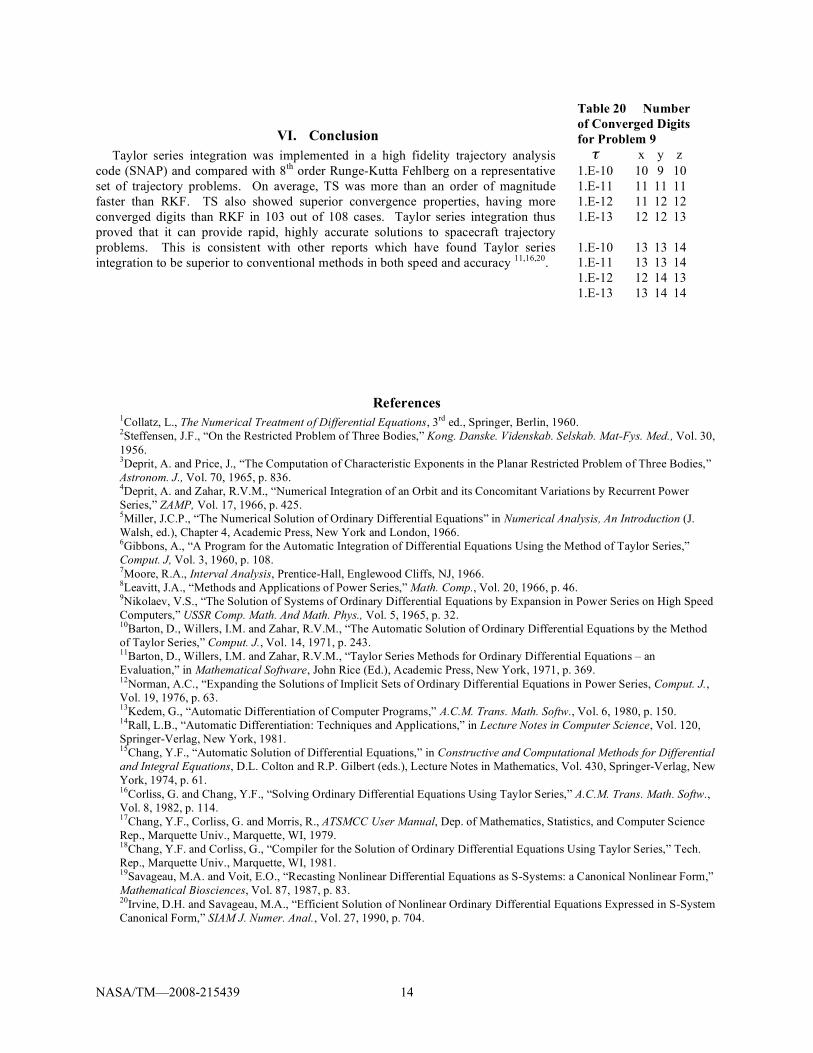
VI. Conclusion Taylor series integration was implemented in a high fidelity trajectory analysis code (SNAP) and compared with 8th order Runge-Kutta Fehlberg on a representative set of trajectory problems. On average, TS was more than an order of magnitude faster than RKF. TS also showed superior convergence properties, having more converged digits than RKF in 103 out of 108 cases. Taylor series integration thus proved that it can provide rapid, highly accurate solutions to spacecraft trajectory problems. This is consistent with other reports which have found Taylor series integration to be superior to conventional methods in both speed and accuracy 11,16,20.

References 1Collatz, L., The Numerical Treatment of Differential Equations, 3rd ed., Springer, Berlin, 1960. 2Steffensen, J.F., “On the Restricted Problem of Three Bodies,” Kong. Danske. Videnskab. Selskab. Mat-Fys. Med., Vol. 30, 1956. 3Deprit, A. and Price, J., “The Computation of Characteristic Exponents in the Planar Restricted Problem of Three Bodies,” Astronom. J., Vol. 70, 1965, p. 836. 4Deprit, A. and Zahar, R.V.M., “Numerical Integration of an Orbit and its Concomitant Variations by Recurrent Power Series,” ZAMP, Vol. 17, 1966, p. 425. 5Miller, J.C.P., “The Numerical Solution of Ordinary Differential Equations” in Numerical Analysis, An Introduction (J. Walsh, ed.), Chapter 4, Academic Press, New York and London, 1966. 6Gibbons, A., “A Program for the Automatic Integration of Differential Equations Using the Method of Taylor Series,” Comput. J, Vol. 3, 1960, p. 108. 7Moore, R.A., Interval Analysis, Prentice-Hall, Englewood Cliffs, NJ, 1966. 8Leavitt, J.A., “Methods and Applications of Power Series,” Math. Comp., Vol. 20, 1966, p. 46. 9Nikolaev, V.S., “The Solution of Systems of Ordinary Differential Equations by Expansion in Power Series on High Speed Computers,” USSR Comp. Math. And Math. Phys., Vol. 5, 1965, p. 32. 10Barton, D., Willers, I.M. and Zahar, R.V.M., “The Automatic Solution of Ordinary Differential Equations by the Method of Taylor Series,” Comput. J., Vol. 14, 1971, p. 243. 11Barton, D., Willers, I.M. and Zahar, R.V.M., “Taylor Series Methods for Ordinary Differential Equations – an Evaluation,” in Mathematical Software, John Rice (Ed.), Academic Press, New York, 1971, p. 369. 12Norman, A.C., “Expanding the Solutions of Implicit Sets of Ordinary Differential Equations in Power Series, Comput. J., Vol. 19, 1976, p. 63. 13Kedem, G., “Automatic Differentiation of Computer Programs,” A.C.M. Trans. Math. Softw., Vol. 6, 1980, p. 150. 14Rall, L.B., “Automatic Differentiation: Techniques and Applications,” in Lecture Notes in Computer Science, Vol. 120, Springer-Verlag, New York, 1981. 15Chang, Y.F., “Automatic Solution of Differential Equations,” in Constructive and Computational Methods for Differential and Integral Equations, D.L. Colton and R.P. Gilbert (eds.), Lecture Notes in Mathematics, Vol. 430, Springer-Verlag, New York, 1974, p. 61. 16Corliss, G. and Chang, Y.F., “Solving Ordinary Differential Equations Using Taylor Series,” A.C.M. Trans. Math. Softw., Vol. 8, 1982, p. 114. 17Chang, Y.F., Corliss, G. and Morris, R., ATSMCC User Manual, Dep. of Mathematics, Statistics, and Computer Science Rep., Marquette Univ., Marquette, WI, 1979. 18Chang, Y.F. and Corliss, G., “Compiler for the Solution of Ordinary Differential Equations Using Taylor Series,” Tech. Rep., Marquette Univ., Marquette, WI, 1981. 19Savageau, M.A. and Voit, E.O., “Recasting Nonlinear Differential Equations as S-Systems: a Canonical Nonlinear Form,” Mathematical Biosciences, Vol. 87, 1987, p. 83. 20Irvine, D.H. and Savageau, M.A., “Efficient Solution of Nonlinear Ordinary Differential Equations Expressed in S-System Canonical Form,” SIAM J. Numer. Anal., Vol. 27, 1990, p. 704.


NASA/TM—2008-215439 14

21Stanford, R.H., Berryman, K.W. and Breckheimer, P.J., “Application of Taylor’s Series to Trajectory Propagation,” AIAA Paper 86-2166, AIAA/AAS Astrodynamics Conference, 1986. 22Berryman, K.W., Stanford, R.H and Breckheimer, P.J., “The ATOMFT Integrator: Using Taylor Series to Solve Ordinary Differential Equations,” AIAA Paper 88-4217-CP, AIAA/AAS Astrodynamics Conference, 1988. 23Gofen, A., “The Modern Taylor Method Package,” URL, http://www.ski.org/Rehab/MacKeben/gofen/TaylorMethod.htm 24Gofen, A., “Interactive Environment for the Taylor integration (in 3D Stereo),” Proceedings of the 2005 International Conference on Scientific Computing CSC’05, 2005. 25Scott, J.R., “Solving ODE Initial Value Problems With Implicit Taylor Series Methods,” NASA TM 2000-209400, 2000. 26Martini, M., “S.N.A.P. 2.3 User’s Manual,” Analex Corporation, Glenn Research Center, Cleveland, OH, 2005.

27Fehlberg, E., “Classical Fifth-, Sixth-, Seventh-, and Eighth-Order Runge-Kutta Formulas with Stepsize Control,” NASA TR R-287, October, 1968. 28Hairer, E., Norsett, S.P. and Wanner, G., Solving Ordinary Differential Equations I, 2nd ed., Springer Series in Computational Mathematics, Springer-Verlag, New York, 1987, p. 168.

29Corliss, G. and Lowery, D., “Choosing a stepsize for Taylor series methods for solving ODE’s,”J.Comp. and Applied Math., Vol. 3, No. 4, 1977, p. 251.

NASA/TM—2008-215439 15

REPORT DOCUMENTATION PAGE Form Approved OMB No. 0704-0188

The public reporting burden for this collection of information is estimated to average 1 hour per response, including the time for reviewing instructions, searching existing data sources, gathering and maintaining the data needed, and completing and reviewing the collection of information. Send comments regarding this burden estimate or any other aspect of this collection of information, including suggestions for reducing this burden, to Department of Defense, Washington Headquarters Services, Directorate for Information Operations and Reports (0704-0188), 1215 Jefferson Davis Highway, Suite 1204, Arlington, VA 22202-4302. Respondents should be aware that notwithstanding any other provision of law, no person shall be subject to any penalty for failing to comply with a collection of information if it does not display a currently valid OMB control number. PLEASE DO NOT RETURN YOUR FORM TO THE ABOVE ADDRESS. 1. REPORT DATE (DD-MM-YYYY) 01-08-2008

2. REPORT TYPE Technical Memorandum

3. DATES COVERED (From - To)

4. TITLE AND SUBTITLE High Speed Solution of Spacecraft Trajectory Problems Using Taylor Series Integration

5a. CONTRACT NUMBER

5b. GRANT NUMBER

5c. PROGRAM ELEMENT NUMBER

6. AUTHOR(S) Scott, James, R.; Martini, Michael, C.

5d. PROJECT NUMBER

5e. TASK NUMBER

5f. WORK UNIT NUMBER WBS 526282.01.03.01.02.01.06

7. PERFORMING ORGANIZATION NAME(S) AND ADDRESS(ES) National Aeronautics and Space Administration John H. Glenn Research Center at Lewis Field Cleveland, Ohio 44135-3191

8. PERFORMING ORGANIZATION REPORT NUMBER E-16609

9. SPONSORING/MONITORING AGENCY NAME(S) AND ADDRESS(ES) National Aeronautics and Space Administration Washington, DC 20546-0001

10. SPONSORING/MONITORS ACRONYM(S) NASA

11. SPONSORING/MONITORING REPORT NUMBER NASA/TM-2008-215439

12. DISTRIBUTION/AVAILABILITY STATEMENT Unclassified-Unlimited Subject Categories: 13 and 64 Available electronically at http://gltrs.grc.nasa.gov This publication is available from the NASA Center for AeroSpace Information, 301-621-0390

13. SUPPLEMENTARY NOTES

14. ABSTRACT Taylor series integration is implemented in a spacecraft trajectory analysis code – the Spacecraft N-body Analysis Program (SNAP) – and compared with the code’s existing eighth-order Runge-Kutta Fehlberg time integration scheme. Nine trajectory problems, including near Earth, lunar, Mars and Europa missions, are analyzed. Head-to-head comparison at five different error tolerances shows that, on average, Taylor series is faster than Runge-Kutta Fehlberg by a factor of 15.8. Results further show that Taylor series has superior convergence properties. Taylor series integration proves that it can provide rapid, highly accurate solutions to spacecraft trajectory problems. 15. SUBJECT TERMS Taylor series; Spacecraft trajectory; Runge-Kutta method; Trajectory analysis; SNAP; Numerical integration; High order

16. SECURITY CLASSIFICATION OF: 17. LIMITATION OF ABSTRACT UU

18. NUMBER OF PAGES

21

19a. NAME OF RESPONSIBLE PERSON STI Help Desk (email:[email protected])

a. REPORT U

b. ABSTRACT U

c. THIS PAGE U

19b. TELEPHONE NUMBER (include area code) 301-621-0390

Standard Form 298 (Rev. 8-98)Prescribed by ANSI Std. Z39-18

high speed solution of spacecraft trajectory problems

Documents