Histopathology Image analysis andNLP for Digital Pathology

by

Aishwarya Krishna Allada

A thesispresented to the University of Waterloo

in fulfillment of thethesis requirement for the degree of

Master of Applied Sciencein

Electrical and Computer Engineering

Waterloo, Ontario, Canada, 2021

© Aishwarya Krishna Allada 2021

Author’s Declaration

This thesis consists of material all of which I authored or co-authored: see Statementof Contributions included in the thesis. This is a true copy of the thesis, including anyrequired final revisions, as accepted by my examiners.

I understand that my thesis may be made electronically available to the public.

ii

Statement of Contributions

Chapter 6 is based on the following paper:

• Aishwarya Krishna Allada and Yuanxin Wang and Veni Jindaland Babaie Mortezaand Hamid Reza Tizhoosh and Mark Crowley. “Analysis of Language Embeddingsfor Classification of Unstructured Pathology Reports”. (Accepted to 43rd AnnualInternational Conference of the IEEE Engineering in Medicine & Biology Society(EMBC) 2021)

I have contributed to implementation, experimentation, and preparation of the manuscriptof the above mentioned paper

iii

Abstract

Information technologies based on ML with quantitative imaging and texts are playing anessential role particularly in general medicine and oncology. DL in particular has demon-strated significant breakthroughs in Computer Vision and NLP which could enhance diseasedetection and the establishment of efficient treatments. Furthermore, considering the largenumber of people with cancer and the substantial volume of data generated during cancertreatment, there is a significant interest in the use of AI to improve oncologic care.

In digital pathology, high-resolution microscope images of tissue samples are storedalong with written medical reports in databases which are used by pathologists. Thediagnosis is made through tissue analysis of the biopsy sample and is written as a briefunstructured report which is stored as free text in Electronic Medical Record (EMR)systems. For the transition towards digitization of medical records to achieve its maximumbenefits, these reports must be accessible and usable by medical practitioners to easilyunderstand them and to help them precisely identify the disease.

Concerning the histopathology images, which is the basis of diagnosis and study ofdiseases of the tissues, image analysis helps us identify the disease’s location and allowsus to classify the type of cancer. Recently, due to the abundant accumulation of WSIs,there has been an increased demand for effective and efficient gigapixel image analysis,such as computer-aided diagnosis using DL techniques. Also, due to high diversity ofshapes and structures in WSIs, it is not possible to use conventional DL techniques forclassification. Though computer-aided diagnosis using DL has good prediction accuracy,in the medical domain, there is a need to explain the prediction of the model to have abetter understanding beyond standard quantitative performance evaluation.

This thesis presents three different findings. Firstly, I provide a comparative analysisof various transformer models such as BioBERT, Clinical BioBERT, BioMed-RoBERTaand TF-IDF and our results demonstrates the effectiveness of various word embeddingtechniques for pathology reports in the classification task. Secondly, with the help of slidelabels of WSIs, I classify them to their disease types, with an architecture having attentionmechanism and instance-level clustering. Finally, I introduced a method to fuse the featuresof the pathology reports and the features of their respective images. I investigated theeffect of combination of the features in the classification of both histopathology imagesand their respective reports simultaneously. This proved to be better than the individualclassification tasks achieving an accuracy of 95.73%.

iv

Acknowledgements

Writing this thesis has been fascinating and extremely rewarding.

I would like to sincerely thank my supervisor, Dr. Mark Crowley, who made this thesispossible by providing his constant support, encouragement, patience, valuable researchdirection and insight throughout my degree. I am glad to be part of his lab, UWECEML,where so many researchers are free to explore creative ideas.

I would also like to thank Prof. Hamid Tizhoosh and Dr. Morteza Babaie for theirconstant support and guidance for my experiments.

I am also thankful to Prof. Hamid Tizhoosh and Prof. Olga Vechtomova for taking thetime to provide an in-depth review of the thesis and provide very helpful feedback. Yourefforts and support are deeply appreciated.

Last but not least, thanks to my parents, brother and grandparents. The support theyshowed me during my research and thesis is the reason I could achieve this milestone.

v

Dedication

This thesis is dedicated to my parents, Srinivasa Rao Allada and Madhavi Allada, forraising me to value education and their unconditional love, no matter the circumstances.To my brother, Rahul Kishan Allada for his infinite support and motivation and my grand-parents - Adatrow Gurunath and Sridevi for their care, affection and encouragement.

To my companion, Chanakya Jetti, who gave me the warmth of a family, away fromhome and for being my constant support system. You are one of the best things that havehappened in my life.

vi

Table of Contents

List of Figures x

List of Tables xii

List of Abbreviations xiii

1 Introduction 1

1.1 Classification of Pathology Reports . . . . . . . . . . . . . . . . . . . . . . 2

1.2 Classification of Histopathology Images . . . . . . . . . . . . . . . . . . . . 4

1.3 Combined Classification of Histopathology Images and Pathology Reports 4

2 Background 6

2.1 Machine Learning . . . . . . . . . . . . . . . . . . . . . . . . . . . . . . . . 6

2.1.1 Supervised Learning . . . . . . . . . . . . . . . . . . . . . . . . . . 7

2.1.2 Unsupervised Learning . . . . . . . . . . . . . . . . . . . . . . . . . 7

2.2 Deep Learning . . . . . . . . . . . . . . . . . . . . . . . . . . . . . . . . . . 8

2.2.1 Introduction to Neural Networks . . . . . . . . . . . . . . . . . . . 8

2.2.2 Recurrent Neural Networks . . . . . . . . . . . . . . . . . . . . . . 11

2.2.3 Long Short-Term Memory . . . . . . . . . . . . . . . . . . . . . . . 12

2.3 Regularization . . . . . . . . . . . . . . . . . . . . . . . . . . . . . . . . . . 14

2.3.1 Dropout . . . . . . . . . . . . . . . . . . . . . . . . . . . . . . . . . 14

vii

2.3.2 Batch Normalization . . . . . . . . . . . . . . . . . . . . . . . . . . 15

2.4 Sequence to Sequence Models . . . . . . . . . . . . . . . . . . . . . . . . . 16

2.5 Attention Mechanism . . . . . . . . . . . . . . . . . . . . . . . . . . . . . . 16

2.6 Convolution Neural Network . . . . . . . . . . . . . . . . . . . . . . . . . . 17

2.7 Embeddings . . . . . . . . . . . . . . . . . . . . . . . . . . . . . . . . . . . 18

2.7.1 Word Embeddings . . . . . . . . . . . . . . . . . . . . . . . . . . . 18

2.7.2 Visual Embeddings . . . . . . . . . . . . . . . . . . . . . . . . . . . 19

3 Related Work 20

3.1 Medical Image Analysis . . . . . . . . . . . . . . . . . . . . . . . . . . . . 20

3.2 NLP on Medical Textual Data . . . . . . . . . . . . . . . . . . . . . . . . . 22

4 Dataset 24

4.1 Dataset from The Cancer Genome Atlas (TCGA) . . . . . . . . . . . . . . 24

4.2 GDC Data Transfer Tool for Querying Dataset . . . . . . . . . . . . . . . . 24

4.3 Further Extraction of Pathology Reports . . . . . . . . . . . . . . . . . . . 26

5 Transformer Models used for Pathology Reports Classification 28

5.1 BioBERT . . . . . . . . . . . . . . . . . . . . . . . . . . . . . . . . . . . . 29

5.2 Clinical BioBERT . . . . . . . . . . . . . . . . . . . . . . . . . . . . . . . . 30

5.3 BioMed-RoBERTa . . . . . . . . . . . . . . . . . . . . . . . . . . . . . . . 30

5.4 Term Frequency-Inverse Document Frequency . . . . . . . . . . . . . . . . 30

6 Analysis of Language Embeddings for Classification of Unstructured Pathol-ogy Reports 32

6.1 Data Preprocessing . . . . . . . . . . . . . . . . . . . . . . . . . . . . . . . 32

6.2 Experimental Setup . . . . . . . . . . . . . . . . . . . . . . . . . . . . . . . 33

6.3 Evaluation Metrics . . . . . . . . . . . . . . . . . . . . . . . . . . . . . . . 35

6.4 Results . . . . . . . . . . . . . . . . . . . . . . . . . . . . . . . . . . . . . . 36

viii

7 Histopathology Image Classification using Attention Mechanism and In-stance Level Clustering 37

7.1 Computational Hardware and Software . . . . . . . . . . . . . . . . . . . . 37

7.2 Histopathology Image Classification Architecture . . . . . . . . . . . . . . 37

7.3 Pre-processing of Whole Slide Images . . . . . . . . . . . . . . . . . . . . . 38

7.4 Feature Extraction . . . . . . . . . . . . . . . . . . . . . . . . . . . . . . . 40

7.5 Experimental Setup and Training . . . . . . . . . . . . . . . . . . . . . . . 40

7.6 Results . . . . . . . . . . . . . . . . . . . . . . . . . . . . . . . . . . . . . . 42

8 Combined Classification of Histopathology Images and Reports 44

8.1 Feature Extraction from Images . . . . . . . . . . . . . . . . . . . . . . . . 44

8.2 Feature Extraction from Texts . . . . . . . . . . . . . . . . . . . . . . . . . 45

8.3 Experimental Setup . . . . . . . . . . . . . . . . . . . . . . . . . . . . . . . 45

8.4 Results . . . . . . . . . . . . . . . . . . . . . . . . . . . . . . . . . . . . . . 47

9 Conclusions and Future Directions 49

9.1 Conclusions . . . . . . . . . . . . . . . . . . . . . . . . . . . . . . . . . . . 49

9.2 Future Studies . . . . . . . . . . . . . . . . . . . . . . . . . . . . . . . . . . 50

References 51

ix

List of Figures

1.1 Combined Image + Text Model . . . . . . . . . . . . . . . . . . . . . . . . 5

2.1 Perceptron Model . . . . . . . . . . . . . . . . . . . . . . . . . . . . . . . . 9

2.2 Feed Forward Neural Model [7] . . . . . . . . . . . . . . . . . . . . . . . . 10

2.3 An un-rolled Recurrent Neural Network [1] . . . . . . . . . . . . . . . . . . 12

2.4 Long Short-Term Memory Unit [106] . . . . . . . . . . . . . . . . . . . . . 13

2.5 Illustration of Dropout [127] . . . . . . . . . . . . . . . . . . . . . . . . . . 15

2.6 Sequence-to-sequence Model [19] . . . . . . . . . . . . . . . . . . . . . . . . 16

2.7 Convolutional Neural Network Architecture [97] . . . . . . . . . . . . . . . 18

2.8 Word Embeddings [86] . . . . . . . . . . . . . . . . . . . . . . . . . . . . . 19

4.1 Sample Whole Slide Image from the Histopathology Image Dataset . . . . 25

4.2 Sample Pathology Report from the Histopathology Reports Dataset . . . . 27

5.1 Overview of the pre-training and fine-tuning of BioBERT [82] . . . . . . . 29

6.1 Data Preprocessing steps . . . . . . . . . . . . . . . . . . . . . . . . . . . . 33

6.2 Deep Neural Network Topology . . . . . . . . . . . . . . . . . . . . . . . . 34

7.1 A Segmented Pathology Whole Slide Image . . . . . . . . . . . . . . . . . 39

7.2 Downsampled Visualization of Pathology Whole Slide Image . . . . . . . . 39

7.3 Model Architecture with Gated Attention Unit and Instance Level Clustering 40

7.4 Attention Maps of Whole Slide Images . . . . . . . . . . . . . . . . . . . . 43

x

8.1 Architecture of the Combined Model . . . . . . . . . . . . . . . . . . . . . 46

xi

List of Tables

4.1 Total Number of Records based on Primary Site . . . . . . . . . . . . . . . 26

4.2 Total Number of Records based on Disease Type . . . . . . . . . . . . . . . 26

6.1 Evaluation of vectorization methods for the classification of disease typeswith a DNN classifier . . . . . . . . . . . . . . . . . . . . . . . . . . . . . . 36

8.1 Performance accuracy of Histopathology Reports only, Histopathology Im-ages only and their combination . . . . . . . . . . . . . . . . . . . . . . . . 47

8.2 Classification Report of the Image-Text Model . . . . . . . . . . . . . . . . 47

xii

List of Abbreviations

AI Artificial Intelligence iv, 2, 4

ANN Artificial Neural Network 8, 11

ANNs Artificial Neural Networks 6, 8, 17

BERT Bidirectional Encoder Representations from Transformers 23, 29

BioBERT Bidirectional Encoder Representations from Transformers for Biomedical TextMining 28–30, 33, 36

CNN Convolution Neural Network 9, 17, 21, 40, 49

CNNs Convolution Neural Networks 6, 8, 14, 17, 20

CV Computer Vision 4, 6, 11, 17, 21

DL Deep Learning iv, 2, 4, 6, 8, 20, 21, 37

DNN Deep Neural Network xii, 3, 5, 14, 15, 20, 32, 33, 36, 44, 45, 47, 50

GDC Genomic Data Commons 24, 25

GRU Gated Recurrent Unit 12, 16

IDF Inverse Document Frequency 30

LSTM Long Short Term Memory 6, 12, 16

ML Machine Learning iv, 2, 6–8, 18, 20

xiii

NCI National Cancer Institute 24

NHGRI National Human Genome Research Institute 24

NLP Natural language Processing iv, 3, 6, 11, 16–18, 20, 28, 29, 33

OCR Optical Character Recognition 26

PLMs pretrained language models 28

RNN Recurrent Neural network 9, 11, 12

RNNs Recurrent Neural Network 8, 11, 12, 16

SPR Surgical Pathology Reports 23

SSL self-supervised learning 28

TCGA The Cancer Genome Atlas 24

TF–IDF Term Frequency – Inverse Document Frequency 30, 31, 33, 35, 36, 50

TF-IDF Term Frequency-Inverse Document Frequency iv, 3, 28

WSI Whole Slide Image 2, 4, 21, 37–41, 44, 45

WSIs Whole Slide Images iv, 2–4, 21, 37–40, 42, 44

xiv

Chapter 1

Introduction

One of the leading causes of death globally is cancer, a group of diseases characterized byabnormal cell growth and the ability to invade or spread to other parts of the body. Bothresearchers and doctors are facing the challenges of fighting cancer [67]. In the UnitedStates, approximately 1.8 million new cancer cases were diagnosed in 2020, with 606,520cancer deaths. Due to the increase in the mortality rate due to cancer, a rapid advancementconcerning cancer research is being developed [53]. Early identification of cancer is essentialto save the lives of many people. Generally, visual examination and manual techniques areused for cancer diagnosis, where manual interpretation of medical slides is time-consumingand prone to errors. In order to bypass the above cases, in the early 1980s [38], computer-aided diagnosis (CAD) systems were introduced to assist doctors in improving the efficiencyof medical image interpretation.

Histopathology is the analysis and interpretation of size, shape, and patterns presentin the cells and tissues of a patient’s clinical records and other factors to study diseasemanifestation. “Histopathology” evolved from combining two of the major branches of sci-ence, namely, “histology” and “pathology.” While histology involves studying microscopicstructures of tissues, pathology involves the disease diagnosis with the help of microscopicexaminations of surgically removed specimens. Throughout the healthcare delivery system,histopathology is a vital discipline exclusively studied and practiced by pathologists. Theprimary duty is to conduct a microscopic analysis of glass slides containing tissue speci-mens to render pathology reports. The pathology reports created by the pathologist areused for various reasons such as development of a diagnostic plan, screening for diseases,monitoring the disease severity, etc. Understanding and explaining the images of tissuesand cells at high resolutions is the core of histopathology.

1

Digital pathology is a digital version of traditional microscopy that is used to exam-ine glass pathology slides. Though Light Microscopy(LM) is considered as the standardreference for diagnosis in pathology, recent developments in ML and AI have drasticallyimproved diagnosing of disease in digital pathology. Thus, in recent times, there has beenan increase in the adoption of digital pathology, with pathology laboratories all over theworld gradually replacing their microscopes with digital scanners and computers.

DL is a type of AI and ML, that imitates the working of human brain in data pro-cessing and creates patterns for decision making. There has been a significant increaseof computational power and recent advancements in the technology of AI, especially DL,which is being used in multiple areas of health care like medical image diagnosis, digi-tal pathology, prediction of hospital admission, drug design, classification of cancer andstromal cells, doctor assistance, etc. [141]. With the advancing technology, the pathologycommunity started digitizing glass slides into gigapixel images through virtual microscopyor Whole Slide Imaging (WSI). The gigapixel images generated via Whole Slide Imagingare the digital slides, and with a large number of increase in digital slides, resulting ina massive creation of databases with WSIs. DL methods, along with their outstandingpattern-recognition capabilities when applied to these digital databases of WSIs, have sig-nificantly increased the value of digital pathology. In addition, computer-aided operationslike segmentation of tissues and cell nuclei and identifying the cancer type and the severityhave become possible after the glass pathology slides have been digitized.

Apart from the digital databases consisting of a massive number of WSIs related tounique cases, each of the WSIs is also accompanied by their respective diagnostic reports,which are written by the pathologists, after the tissue analysis of the biopsy sample. Withthe increase in the applications of Digital Pathology for research and teleconsultation,there is a growing increase in the amount of histopathology data. In this context, thisthesis presents research of applying computer vision, Natural Language Processing andML algorithms for the quantitative image and text-based analysis of histopathology imagesand reports.

1.1 Classification of Pathology Reports

In almost all cases, the diagnosis of a whole slide image WSI is made through tissue analysiswhich is described in a detailed format in a pathology report. Pathology reports holdimportant details of the WSI analysis, which is stored in most electronic medical recordsystems as unstructured free data. A part of clinical research focuses is on the manualextraction of data from pathology reports, which is very expensive and time-consuming.

2

The data helps identify the case, select the treatment and its plan, risk stratification,etc. The electronic medical record systems hold the records of essential details of thepatient’s health and pathologist’s elucidation of the findings from the WSIs. It also hasthe information that helps physicians understand the details of WSIs and records thatinformation for future clinical and research use.

For almost 50 years, researchers have worked to develop Natural Language ProcessingNLP algorithms to extract details from pathology reports. However, only a limited numberof categorical data elements are typically extracted, and model outputs often lack reliableuncertainty estimates, limiting the clinical applicability of these systems and only 10% ofwhich have been reported to be in real-world use [105]. Also, many attempts are being madeto store the pathology report information in a specific template, but most of the informationis recorded in free text. This text is a massive hurdle for immediately extracting andusing the details and information a report holds by clinicians, researchers, and healthcareinformation systems. This ambiguity is due to the complexity of natural language, thecomplexity of pathology images description explained by a variety of sources [54].

Due to the above reasons, the pathology reports are not feasible in using automatedmethods to suggest proper treatment or promote clinical research. On top of that, a mas-sive volume of pathology reports are produced every year. For instance, an average-sizedlaboratory produces more than 50,000 reports annually. Most of these reports have no di-rect connection to the tissue samples. Also, each patient’s report is a customized documentwith high vocabulary discrepancies, such as misspelled words and lack of punctuation. Itis common to find clinical diagnoses intermixed with nuanced explanations and multipleterminologies used to mark the same malignancy and data about various carcinomas ina single report [46]. Cancer registries are facing a considerable challenge in the manualanalysis of the enormous quantity of pathology reports, with the rise in the number of pa-tients with cancer and the improvement in treatment complexity [46] [134]. Moreover, theprocess of figuring out the diseases from a pathology report is challenging, time-consumingand requires extensive training when done manually [46].

The first part of this thesis demonstrates how to extract meaningful numerical embed-dings from written pathology reports to help classify various types of cancer. One of ourresearch’s primary focuses is to evaluate and compare the effectiveness of existing machinelearning methods for the automatic classification of a given pathology report to its respec-tive disease type. We demonstrate that contextualized word embeddings combined withTF-IDF feature vectors, when given as inputs to a DNN, can be an effective method forclassification, achieving 93.77% accuracy in our study. This study proves the competenceof TF-IDF features and its effectiveness in recognizing essential keywords in a pathologyreport. Additionally, our experiments with digital pathology reports will allow researchers

3

to develop a versatile way of extracting essential details from free-text pathology reports,which could benefit various medical diagnostic tasks.

1.2 Classification of Histopathology Images

Histopathology image analysis is used to help pathologists identify tumors and their sub-types and eases pathologist’s workload. The most recent studies in digital pathology havefound that supervised AI algorithms for classification are compelling and vital use of thesedigitized images is used to create diagnostic algorithms or applications which can augmentthe diagnostic workflow. Histopathology WSIs contains a massive number of pixels, wherethese pixels can now become part of a DL algorithm to look for shapes, features or patternsutilizing image analysis, DL and AI tools [61]. DL is at the forefront of CV, showcasingsignificant improvements over previous methodologies on visual understanding [37] of apathology image. The emergence of DL is becoming very beneficial, especially in digitalpathology, where it is practically not very easy to detect, segment and identify a givenWSI having thousands of pixels to a specific disease type.

Recently, the Food and Drug Administration has approved usage of WSIs for primarydiagnosis [108]. On the other hand, though DL is widely used for computer-aided diagno-sis, there is always a trade-off between the accuracy of the model and its interpretability.In addition, General Data Protection Regulation (GDPR) has claimed the “right to ex-planation” for any decision made by artificially intelligent algorithmic systems. Moreover,in the medical domain, the model’s prediction is given more importance than other fieldsbecause any mishap can become fatal for the patient.

The second part of this thesis demonstrates the result of the experiment performed forthe classification of WSIs into their respective cancer types. The experiment is carriedout in a weakly supervised setting with an attention scoring mechanism and instance-levelclustering, yielding an accuracy of 90.12%.

1.3 Combined Classification of Histopathology Images

and Pathology Reports

Both images and texts are essential for human intelligence to understand the real world.Many types of researches [43, 48, 83] were performed to bridge these two modalities. Inorder to investigate the effectiveness of combining image and language to predict and gain

4

Figure 1.1: Combined Image + Text Model

insight, we proposed a method to classify the histopathology images by using associatedmetadata, i.e., their associated reports as shown in Figure 1.1. Intending to classify bothhistopathology reports and images together as they contain complementary information,the proposed method combines the features of the report’s texts and images from theexperiments in section 1.1 and section 1.2. These concatenated images and text featuresare used to classify images and reports using a DNN classifier. The experiment provedthat the combination of features gave comparatively good accuracy of 95.7% compared tothe individual experiments on histopathology reports and images, respectively.

5

Chapter 2

Background

This chapter explains some of the components and building blocks used in our experiments.Firstly, various classes of ML models are outlined, after which we introduce Deep LearningDL and ANNs. We also introduce CNNs, class of ANNs which are generally used in CVand NLP literature and also LSTM networks, which are generally used in NLP literature.Also, theory regarding regularization, sequence-to-sequence models, attention mechanismsare introduced as we used them in our image classification model. Also, we brief aboutembeddings, which is an important concept in NLP.

2.1 Machine Learning

Machine Learning ML enables computers to learn from data, without being explicitlyprogrammed, where the data is used to train the system to perform any specific task. InML, model recognizes the patterns and intricacies within the data with the help of someform of mathematical optimization and statistical methods. The trained model can furtherautomate tasks or guide decision-making based on data and the mathematical model.

ML is being used predominantly in our everyday lives and is developing at a fast pace.For example, all the email services use ML to filter out spam emails, while online shoppingprovides us with recommendations that use ML. In addition, several kinds of research arebeing performed daily with new algorithms and methodologies developed and applied inmany areas ranging from the medical field to climate change. These advancements inintelligent systems are beneficial as it makes all the application’s process more accessibleand at the same time with less human intervention.

6

Generally speaking, there are two categories of ML methodologies, which are namelysupervised learning and unsupervised learning, where the primary categorization is basedon the type of learning process carried. The subsection below elaborates on each of thecategories with examples.

2.1.1 Supervised Learning

Supervised learning algorithms are trained with data points containing the features (inputs)and their respective labels (outputs). This algorithm usually modifies the model parametersso that the desired output for a given input is obtained. In this algorithm, we have outputlabels that correspond to each input used to train the model.

Once the model is trained, it is then provided with new unseen data points as inputs,where the model will predict the target based on what it has previously learned. A few ofthe most popular supervised learning algorithms which are commonly used in classificationand regression studies are linear and logistic regression [29], Support Vector Machine [14],Naive Bayes Classifier [98], Gradient Boosting [15], [44], classification trees, and randomforest [16], [112].

To better understand the supervised learning method, let us consider an example withthe image classification task. Initially, we feed the ML model with images of GoldenRetriever, huskies, poodles, etc. and label them as dogs. Similarly, we can provide imagesof Persian, Maine, British shorthair, etc., all labeled as cats. Given the input images andthe respective labels, the model tries to learn from the image pixel the characteristics thatdifferentiate dogs from cats. Once after training, the model is then used to classify newimages.

2.1.2 Unsupervised Learning

Unsupervised learning algorithms are fed with training data points containing the features(inputs) and do not require pre-existing output/labels. These algorithms can identifyhidden patterns based on the distribution of the input data. This learning method can beused for detecting anomalies, wherein some parts of the data may not fit well with the restof the data. One of the most common unsupervised learning methods is Clustering (e.g.,hierarchical clustering [122], [34], K-means [89], [96]) and few other popular approachesare Latent Dirichlet Allocation (LDA)[12], principal component analysis (PCA) [45] andword2vec [102].

7

For example, suppose we train a model with unlabelled documents related to varioustopics like sports, politics, movies, etc. In that case, a model will automatically clustersimilar documents that belong to similar topics, with the information provided in thedocuments, such as word usage and writing style.

2.2 Deep Learning

ANNs are an important class of machine learning models, used for both supervised andunsupervised tasks, where biological neural networks inspire the structure and their func-tioning. The brain consists of billions of interconnected neurons, which ANNs try to mimic.ANNs have multiple layers with simple processing units known as nodes where each of themare connected by edges with weights [51].

Recently, there has been an increasing interest in neural network architectures consistingof many layers. With the availability of a large volume of data and powerful hardware forcomputation, such model architectures were able to outperform humans in several cognitivetasks [119][104]. This led to the creation of a sub-field of ML known as DL [81].

The most basic version of an ANN model is a feed-forward neural network, where thereexist other architectures such as RNNs, CNNs, etc., which are explained in detail in thesections below.

2.2.1 Introduction to Neural Networks

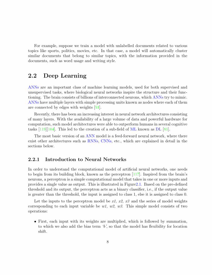
In order to understand the computational model of artificial neural networks, one needsto begin from its building block, known as the perceptron [117]. Inspired from the brain’sneurons, a perceptron is a simple computational model that takes in one or more inputs andprovides a single value as output. This is illustrated in Figure2.1. Based on the pre-definedthreshold and its output, the perceptron acts as a binary classifier, i.e., if the output valueis greater than the threshold, the input is assigned to class 1, else it is assigned to class 0.

Let the inputs to the perceptron model be x1, x2, x3 and the series of model weightscorresponding to each input variable be w1, w2, w3. This simple model consists of twooperations:

• First, each input with its weights are multiplied, which is followed by summation,to which we also add the bias term ‘b’, so that the model has flexibility for locationshift.

8

• Next, a class label (0 or 1) is assigned based on a binary activation function.

Figure 2.1: Perceptron Model

The predicted value of output y corresponding to the given set of inputs, and in orderfor the predicted output to be close to the desired output (ground truth), we would needto make adjustments to the weights w1, w2, w3 and bias term b.

However, with the recent advancements, modern neural networks do not use the simpleperceptron anymore. Instead, they consist of computational units known as neurons (ornodes), which replace the simple binary activation function with non-linear functions,combining multiple layers of neurons to form a more robust model known as the feed-forward neural network is possible. Each neuron is connected to every other neuron inthe previous and subsequent layers. However, there are no connections between neuronswithin the same layer.

As illustrated in Figure 2.2, there can be multiple inputs and multiple outputs wherethey are connected via several hidden layers. The input at each neuron gets transformedby weighted summation followed by non-linear activation. The computation starts fromthe input layer until the output layer and is known as forward propagation. Feed-forwardneural networks are often used for transforming the dimension of inputs and outputs ofdifferent complex models like CNN and RNN. They can learn non-linear representationsof the data and have been successfully applied to many classification and regression tasks.

The non-linear activation functions can be different in each layer of the network. How-ever, while all the hidden layers have a similar activation function, the final layer can have

9

Figure 2.2: Feed Forward Neural Model [7]

a different one. Thus, there are many choices of activation functions, and some of themare listed below:

• ReLU: ReLU is known as rectified linear unit, is a popular activation function, whichis known for its simple computations. A ReLU function simply returns the input ifthe input is bigger than one, and zero otherwise:

f(x) =

{x if x>0

ax otherwise(2.1)

The derivatives of ReLU activation function are computed with significantly lesscomputational power, where it is 1 for values above 0 and 0 otherwise.

• Sigmoid: A sigmoid activation function has an S-shaped curve, and it clips the value

10

of input between 0 and 1.

f(x) =1

1 + e−x=

ex

ex + 1

• Softmax: Softmax activation function is mainly used when the output of a neuralnetwork is a vector, and the goal is to pick the most probable component. Thisfunction amplifies the maximum value in a vector or an array and lessens or dampensthe rest of the components’ values.

σ(z)i =ezi∑Kj=1 e

zifor i = i, ...Kand z = (z1, ...zk) ∈ RK

• Tanh: Tanh activation function is also known as hyperbolic tangent ActivationFunction, which is similar to sigmoid activation function, but ranging from -1 to +1.

tanhx =sinhx

coshx=ex − e−x

ex + e−x

With no structured methodology to adjust the model weights, other than by trial anderror, there has been significant research [135, 118], which contributed to the developmentof the method known as backpropagation of errors, which made it possible to estimatethe weights in an ANN model. Backpropagation computes the gradient of the network toindividual connection weights, given a loss function, such as the mean squared error (MSE)loss.

2.2.2 Recurrent Neural Networks

Recurrent Neural Networks (RNN) is a type of neural network model which can handlevariable-length data. Each RNN unit has a self-loop and an internal state which helpsprocess sequential data like audio waveform, stock value, text and video. RNNs helpprocess sequential data because they can utilize each data point as well as the relationof that data point with the preceding data points, which results in generating a morecomprehensive and proper textual representation. As a result of their usefulness, RNNsare used in NLP and CV for various tasks [139].

Figure 2.3 shows an RNN network, where xi denotes the input to an RNN which isusually the feature vector and hi denotes the hidden state carried forward and outputted

11

Figure 2.3: An un-rolled Recurrent Neural Network [1]

at each time-step by the RNN. This figure denotes the simplest form of RNN. In practicewe often use a LSTM [56] or GRU [36] network. Both these networks are complex andperform much better at language tasks. They consist of internal states and gates combinedwith non-linearities to allow better learning of complex functions and mappings.

2.2.3 Long Short-Term Memory

As described in the previous section, RNNs learn representations of the data over temporalsequences, like text or audio features. However, in practice, RNNs do not seem to assignpriorities to which of the past data they choose to ascribe higher importance, which isdetrimental to their usage in tasks that require the processing of long sequences of datalike in text, audio or video processing. This lack of ability to learn long-term dependenciesin the input features is shown in previous work by [8]. LSTM seeking to address this issueby explicitly modeling how much to retain and forget at each time-step during the RNNstraining procedure.

The structure of an LSTM is depicted in Figure 2.4. An LSTM unit is comprised ofthree distinct gating layers internally - namely, the forget gate, input gate and output gate- that determine its outputs: the new cell state and hidden state. The three gates areenclosed within a “cell” that remembers relevant information over different time intervalsand regulates the flow of information into and out of the cell. The gating mechanism helpsthe LSTMs to capture distant temporal dependencies.

As can be seen in Figure 2.4, the cell state Ct passes through the LSTM mostly unper-turbed, which is intended to address the problem of vanishing gradients. The forget gate

12

Figure 2.4: Long Short-Term Memory Unit [106]

uses a sigmoid activation to squash the output values of the previous time step between 0and 1, which can be understood as being semantically equivalent to deciding how much ofthe previous cell state to forget.

f t = σ(W f · [ht-1, xt] + bf)

The input gate also uses a sigmoid activation on the previous hidden state, which ismultiplied by the candidate cell state C. The value thus obtained is then multiplied by theforget-gated previous cell state to form the next cell state.

13

it = σ(W i · [ht-1, xt] + bc)

Ct = tanh(W c · [ht-1, xt] + bc)

Ct = f t · Ct-1 + it · Ct

Now that we have obtained the cell state, we propagate that through to the next timestep. To obtain the hidden state, we use an output gate, again with a sigmoid activation,to gate the cell-state and create the hidden state for the next time step.

ot = σ(W o · [ht-1, xt] + bo)

ot = tanh(Ct)

LSTMs outperform simple recurrent neural networks in learning long-term dependen-cies, making them suitable for various natural language processing tasks. LSTMs have alsobeen combined with other types of neural networks, such as CNNs, to improve automaticimage captioning [90].

2.3 Regularization

Regularization refers the technique used in machine learning models to improve the model’sgeneralization capabilities. A few of the techniques are early stopping, dropout, parameternorm penalties, etc.

2.3.1 Dropout

One of the most common problems faced by DNN architectures is overfitting, which refersto the problem of a model learning functions that represent the training set very well butfail to generalize to the validation/test set. Dropout is used as a regularization techniqueto help mitigate the problem of overfitting [127].

Using dropout, neurons and their connections are randomly dropped during training,where each neuron can be dropped with a fixed probability that is a tunable hyperparame-ter. Using dropout in DNN helps the model prevent overfitting by limiting the development

14

Figure 2.5: Illustration of Dropout [127]

of excessive codependency between units during training. We should remember that duringthe testing/inference step, no neurons are to be dropped. Figure 2.5 illustrates the ideabehind dropout.

2.3.2 Batch Normalization

The batch normalization [64] technique is used to improve the training speed and stability ofDNN, which works by reducing internal covariate shift. Internal covariate shift is definedas the change in the distribution of the network unit outputs due to the change in thenetwork parameter values, and the reduction is obtained through batch normalizationtransformation of a layer’s input defined as:

y =x− E[x]√V ar[x]

· γ + β

where x is the layer inputs and γ, β are learnable parameter.

15

2.4 Sequence to Sequence Models

Sequence-to-sequence (Seq2Seq) [128] models are mostly made up of an encoder and a de-coder, which is predominantly used in Natural Language Processing (NLP) and is mainlyused to convert a random input sequence to an output sequence. The sequence can rangefrom whole documents to individual words. Both the encoder and the decoder are usuallyimplemented with RNNs (usually an LSTM or GRU), where the encoder learns an inter-mediate representation of the input sequence, which the decoder will use to generate thedesired output sequence. An overview of a seq2seq network used for translation is shownin Figure 2.6.

Figure 2.6: Sequence-to-sequence Model [19]

2.5 Attention Mechanism

Attention is a technique that imitates cognitive attention. Likewise, attention mechanismis used in neural networks to help the training process by indicating to the model whatpart of the inputs or features are to be focused upon. Here we will discuss the attentionmechanism used in Natural Language Processing and Computer Vision.

In NLP, two popular attention mechanisms used in Seq2Seq models are Luong Attention[94] and Bahdanau Attention [6], which were introduced for machine translation, which

16

outperformed vanilla Seq2Seq models. This attention is obtained by aligning tokens onthe target side to the tokens on the source side. The attention mentioned in the abovemechanisms used in Seq2Seq models differ in how the context vector is computed whereLuong Attention takes a multiplicative form. In contrast, the Bahdanau Attention takesan additive form.

On the other hand, the attention mechanism was found to be helpful in CV especiallyin image captioning [137] and object detection [13]. Using the whole image in any task,for instance, in a classification task, will lead to significant noise, thus lowering detectionaccuracy. Also, in medical images, where the medical images are made up of thousands ofpixels, identifying the lesion area, which may be small, will be difficult, given the entireimage [49]. Recursive hard attention[49] is used by cropping out the discriminative partsof the image and classifying both the global image as well as the cropped portion together.While attention reweighs certain network features, soft attention allows these weights tobe continuous while hard attention requires them to be binary.

2.6 Convolution Neural Network

CNNs are a class of ANNs most popularly used for visual analysis, and in simple terms,CNNs are regularized multilayer perceptron (MLP). CNNs use the convolution operationin at least one of their layers instead of general matrix multiplication. While multilayerperceptron (MLP) is prone to over-fitting due to their fully connected nature, CNNs usesmall and simple patterns to learn more extensive and more complex patterns in data,resulting in less connections and lower complexity.

An input layer, output layer and hidden layer are the three types of layers in CNNs. Thehidden layers consist of a series of convolution operations, which convolve with an operationsuch as multiplication or dot product. These layers are commonly followed by additionalconvolutional layers, such as pooling and fully connected layers. The pooling layers reducedata dimension by reducing outputs from a group of data points to a single value. Differentpooling operations result in different types of features. Global pooling [23], max-pooling[24], and average pooling [103] are the most common pooling operation employed. Figure2.7 shows an overview of a simple CNN. Even though CNNs was primarily introduced inthe computer vision community, they have been extensively explored for many NLP tasks[26].

17

Figure 2.7: Convolutional Neural Network Architecture [97]

2.7 Embeddings

In ML, embeddings mean the mapping of discrete variables to a vector in continuous space.The vectors partially represent the semantics of the raw input data, which otherwise maynot be easily comprehensible to a neural network. For example, we cannot directly traina neural network for image classification with the image pixels without transforming itinto embedding space. We discuss embeddings for inputs from words and images in thefollowing subsections.

2.7.1 Word Embeddings

In NLP, word embeddings are the vector representation of all the words in the vocabulary.Techniques used to learn word embeddings are unsupervised, though supervised and semi-supervised techniques have also been proposed. The embeddings are learned so that wordsappearing in similar contexts are close to each other. For example, words like “grapes” and“banana” will appear close to each other as they belong to the family of fruits. Figure 2.8shows word embedding space. Various techniques like Word2vec [101], Glove [109], ELMo[110], FastText [70], Skip-thoughts [76], Quick-thoughts [91], InferNet [27], and Google’suniversal sentence encoder [18].

18

Figure 2.8: Word Embeddings [86]

2.7.2 Visual Embeddings

The main goal for pre-trained embeddings for visual modality is to learn a meaningfulrepresentation of images, though the methods used to learn those embeddings are notcompletely supervised. Pre-trained visual embeddings are nothing but the feature vectorsextracted from the hidden layers of a neural network trained on any task. For example, afew popular choices of obtaining pre-trained image embeddings are Inception [130], VGG[123], SqueezeNet [57], and DeepLoc [79], are all trained on an image classification task.

Learning a joint representation of visual and other modalities like speech and wordembeddings is still an active field of research.

19

Chapter 3

Related Work

In recent years, there has been ongoing research in applying ML methods to medical imagesand texts. Medical images pose unique challenges due to their significant variations, richstructures, and large dimensionality. On the other hand, electronic health records arechallenging as they are highly unstructured, with many medical terminologies present inthe text. As a result, researchers have begun to look into various image and text analysistechniques, and their applications in digital pathology [50].

The first section in this chapter briefs on a few of the past works done on the medicalimages. In contrast, the second section discusses the previous NLP techniques used inmedical text data.

3.1 Medical Image Analysis

Recently, DL based approaches were performing better than conventional machine learningmethods in image analysis tasks, automating end-to-end processing [21, 58, 60]. The maingoal of histopathology is to differentiate between normal tissue, non-malignant and ma-lignant lesions and to perform a prognostic evaluation [40]. Considering medical imaging,CNNs have been successful in diabetic retinopathy screening [113], bone disease prediction[132] and age assessment [59], and other problems [21]. DNN models achieved massive suc-cess in achieving state-of-the-art resulting in histopathology image analysis from diseasegrading, cancer classification to outcome prediction [126, 10, 87].

Lately, self-supervised and semi-supervised approaches are becoming increasingly pop-ular to reduce the annotation burden by leveraging the readily available unlabeled data

20

that can be trained with limited supervision. Promising results for the above methods inCV is seen in [69, 80, 124] and medical image analysis tasks [20, 131, 84].

Initially, most of the DL training on WSIs did not use the whole image as input; instead,they divided the WSIs into multiple patches and used those patches for training the model[66, 39, 17, 4]. Since the patch size is tiny compared to the complete WSI, there arelarge amounts of background regions that are useless for diagnosis. Hence it is essentialto remove the background regions. However, this problem is often treated as a trivialpart of the research, mostly solved via threshold-based methods. In [68] a threshold wasused on the pixel intensity values to detect the tissue. As another example, [78] removedblank regions by setting a threshold on saturation and intensity of pixels. Other worksused homogeneity criteria to only select patches containing a considerable part of the tissue[41]. Apart from threshold-based methods, [115] discusses different U-Net, a light weightedCNN architectures to segment only the tissue region from the background.

Concerning the pre-processing in medical images, one of the main steps followed inWSIs is color normalization of stained tissue samples [39]. Despite the standardized stain-ing protocols, versions in the staining outcomes are prevalent due to variations within thestaining parameters, e.g., Antigen awareness and incubation time and temperature, excep-tional situations among slide scanners, etc. [140]. Such color versions can adversely affectthe performance and accuracy of the classifier. Therefore, in these papers [65, 74, 85, 95]stain normalization techniques have been proposed for better performance of the model.One of the most frequent ways to remove the stains from the patches is to transform thecolor appearance of a source image to the target image [133] and [114] presents a methodto transform the color appearance of a source image to the target image.

An efficient classification model was built [77] where the input size equals the patchsize and inception-v3 network is used as the classifier and is trained them from scratchwith an input size of 512 x 512 to detect and discriminate epithelial tumors in WSIs ofstomach and colon and achieved an accuracy of 95.6%. On the other hand, [5] have useda slightly different CNN model, which was architecturally and conceptually inspired byAlexNet and VGG16 on a new dataset named “Kimia Path24” and achieved an accuracyof 44.80%. However, [75] has used the same “Kimia Path24” dataset and has comparedthe performance of DenseNet-161 and ResNet-50 pre-trained CNN models. The resultsproved that ResNet-50 obtained a validation accuracy of 97.77% which was better thanthe 95.79% achieved by DenseNet-161.

Once after classifying the WSIs, it is essential to explain the model’s prediction to justifytheir reliability, and more importance is given to the model’s interpretability when it comesto the medical domain. The paper [93] defines a suitable measure of feature importance in

21

the SHAP (SHapley Additive exPlanations) framework. LIME [116] explains the choice byhighlighting or segmenting the critical region in the particular patch on which the classifiermade the decision, thus helping the practitioners to validate the model. In the paper,[138] heatmap is drawn based on confidence scores of each patch, based on which theinterpretability of the model is explained.

In this thesis, I present an approach for histopathology microscopy image analysis forcancer type classification. Our approach is by using a weakly supervised method usinginstance-level clustering and attention mechanism.

3.2 NLP on Medical Textual Data

In the field of biomedical research, information extraction using NLP spans from rule-basedsystems [73] down to domain-specific systems using feature-based classification [134], andto the recent deep networks for end-to-end feature extraction and classification [46].

Several studies performed for information extraction techniques from pathology reportsbelonging to various types of tumor related to lungs, breast, colorectal, prostate, where[125] mentioned the overview of various tools developed. [25] performed an experimentto automatically extract diseases from pathology reports belonging to colon cancer. Rule-based systems in combination with machine learning methods were used to extract ninedifferent classes from the reports.

While [107] extracted 28 different concepts from pathology reports for primary cu-taneous melanoma (skin cancer), [99] classified colorectal cancer according to the TNM(Tumor, Node and Metastases) scale using Naıve-Bayes and Support Vector Machines.[100] applied rule-based methods to pathology reports for lung cancer, where the resultsobtained from the experiments gave F1-Score from 0.7 to 0.9.

[31] on the other hand, used rules to extract concepts in 5,826 breast cancer and 2,838prostate cancer pathology reports. The experiment extracted around 80 fields and obtained90-95 percent accuracy, and domain experts evaluated.

Two studies have applied rule-based methods to Norwegian pathology reports on thereports belonging to a language other than English. [32] extracted values for nine conceptsfrom 25 pathology reports describing prostate biopsies, where they obtained F-scores rang-ing from 0.24 to 0.94. On the other hand, [134] extracted values for ten concepts relatedto breast cancer with an F-score ranging from 0.67 to 1.0 using 40 reports. Both studieswere done on small data sets, but the results show that rule-based methods are promisingfor information extraction from pathology reports written in Norwegian.

22

In case of classification tasks or retrieving specific features from reports, successfulstudies in NLP for understanding pathology reports have been reported [63]. For example,The Cancer Text Information Extraction System(caTIES) is a framework developed in acaBIG project [30] that focuses on the extraction of crucial details from SPR to achievehigh precision and recall. On the other hand, a system named Open Registry [28] was ableto filter out the pathology reports having cancer specified in them, based on the diseasecodes.

In 2010, the Automated Retrieval Console(ARC) [33] was introduced, where machinelearning models are used to predict the degree of association of a given radiology or pathol-ogy report to cancer. The performance of this approach varied from an F-measure of 0.75for lung cancer to 0.94 for colon cancer. However, this approach utilized domain-specificrules, which may be disadvantageous when working with a wide variety of pathology re-ports. Other works have performed a classification of the pathology reports by extractingthe TF-IDF features [71]. The extracted features were given as input to XGBoost, SVMand Logistic Regression, where improved ensemble results were obtained with the XGBoostclassifier.

In addition, many algorithms that convert words to fixed-dimensional vectors that canbe used to preserve syntactic and semantic relationships in a text corpus were introduced.These include word2vec [102], and GloVe [109] which use co-occurrences of words in the textand produce dense vectors such that words appearing in similar contexts have similar wordembeddings. Significant improvements that could be achieved in the NLP field came whenunsupervised model architectures were proposed to represent words as a fixed dimensionaldense vector [102], [101]. The architectures were Continuous Bag of Words(CBOW) thatpredicts the target word given the context and the Skip-gram model, which predicts thecontext based on the target word. Another significant advance was BERT [35], which im-proves fine-tuning-based approaches by taking into account both left and the right context,unlike the traditional algorithms, which used the left-to-right direction only.

23

Chapter 4

Dataset

This chapter briefs the dataset used for our experiments and the tool used to extract thehistopathology image and textual data.

4.1 Dataset from The Cancer Genome Atlas (TCGA)

TCGA is a cancer genomics program, having around 20,000 primary cancer and matchednormal samples over 33 cancer types. TCGA is a collaboration between the NCI andNHGRI, which aims to generate comprehensive, multi-dimensional maps of the fundamen-tal genomic changes in major types and subtypes of cancer. TCGA has analyzed matchedtumor and normal tissues from 11,000 patients, allowing for the comprehensive character-ization of 33 cancer types and sub-types, including ten rare cancers and the TCGA data,are hosted at the NCI GDC [121]. In addition, TCGA has the tissue slides and the reportfor different types of cancer for each organ and the tool we used to extract the data isdescribed in the section below.

4.2 GDC Data Transfer Tool for Querying Dataset

The GDC Data Model is the primary method of organizing all data within the GDC, whichcan be thought of as a Directed Acyclic Graph composed of interconnected entities. Anentity in the GDC is a unique component of the GDC Data Model where each entity hasassociated some attributes that can be used to describe it. GDC Data Portal allows the

24

user to filter available data files according to different criteria. The user can downloadfiles individually or add them to the cart while the search is underway. The GDC DataTransfer Tool is a standalone client application that runs on the user’s machine, and ithelps download large volumes of data [121]. Due to the high volume of images to bedownloaded, GDC Data Transfer Tool was used, and a manifest file consisting of all thefiles to be downloaded was provided. A sample pathology image from the dataset can beseen in Figure 4.1.

Figure 4.1: Sample Whole Slide Image from the Histopathology Image Dataset

Among the records, we picked a total of 1949 data points belonging to four primarysites: kidney, lungs, thymus, and testis with 937, 749, 124 and 139 records. Further,seven different diseases types belonging to the above organs are chosen which are namely,“Kidney Renal Papillary Cell Carcinoma”, “Kidney Renal Clear Cell Carcinoma”, “LungAdenocarcinoma”, “Lung Squamous Cell Carcinoma”, “Testicular Germ Cell Tumors”,“Kidney Chromophobe” and “Thymoma”. Amongst the medical reports, the main criteriafor choosing the reports are the quality of the PDF reports. Therefore, only those reportsthat were quite readable were considered, and the rest were discarded. The number ofsamples in each class used for our experiments based on primary site and disease type areas shown in the Tables 4.1 and 4.2.

25

Primary Site Number of sampleskidney 937lungs 749Testis 139

Thymus 124

Table 4.1: Total Number of Records based on Primary Site

Disease Type Number of samplesKidney Renal Clear Cell Carcinoma 537

Lung Adenocarcinoma 372Lung Squamous Cell Carcinoma 356

Kidney Renal Papillary Cell Carcinoma 283Testicular Germ Cell Tumors 139

Thymoma 124Kidney Chromophobe 110

Table 4.2: Total Number of Records based on Disease Type

4.3 Further Extraction of Pathology Reports

Once after selecting 1,949 reports, the next step was to extract the text from those reports.As it is not practical to type the relevant and valid information from those reports manually,which will be extensively time-consuming, OCR was implemented. This software convertedall the PDF reports to text files, which we used for the experiments. Once after convertingthe image data of the reports to text files, manual inspection of spelling errors and grammarwas inspected on those files. Also, irrelevant characters produced as an artifact by the OCRsystem were removed. These cleaned pathology reports are further used for experiments,and an example of a pathology report from the dataset is as shown in Figure 4.2.

26

Figure 4.2: Sample Pathology Report from the Histopathology Reports Dataset

27

Chapter 5

Transformer Models used forPathology Reports Classification

Transformer-based PLMs is made of the combination of transformers with transfer learn-ing, and SSL has been booming in the field of NLP from the past few years. With a greatsuccess of PLMs in the general domain, there was an urge felt in the medical and biomed-ical communities to develop various PLMs in these domains. PLMs can learn languagerepresentations that are useful across tasks, and we can directly use the pre-trained modelwithout training the models from scratch. These PLMs are trained over a huge corpusof unlabelled textual data using a self-supervised learning mechanism, learning betweensupervised and unsupervised learning. In self-supervised learning, as the labels are notcreated manually, they are generated automatically based on the relationship between dif-ferent sections of the input data. Once after the training of the transformer-based PLMsover huge corpora of texts of a specific domain, the models can be further used for multipledownstream tasks just by fine-tuning by adding layers based on the task [35, 72].

Recently, there has been an increasing demand for text mining in the clinical domain,with a considerable increase in the number of biomedical documents produced with es-sential details and information in them. This lead to the generation of lots several PLMseach consisting of millions or even billions of parameters. In this section, we describeseveral contextualized word embedding models trained on biomedical and clinical corporalike BioBERT, Clinical BioBERT and BioMed-RoBERTa along with TF-IDF and theirtechniques to convert text into vectors.

28

5.1 BioBERT

BERT was a state-of-the-art model in NLP, which was proposed by Google researchers,which takes into consideration of the bi-directional context of the text in all the layersof its architecture [35]. These representations are useful for sequential data that dependsheavily on the context in a text. The introduction of transfer learning in this field aidsin carrying encoded information over to strengthen an individual’s smaller tasks acrossdomains. In transfer learning, we refer to this step as “fine-tuning,” and it means that thepre-trained model is now being fine-tuned for the specific task at hand. BERT is originallyan English-language model which was pre-trained using 2.5 billion words from Wikipediaand 0.8 billion words from BooksCorpus corpora. The architecture of BERT is as shownin the figure 5.1.

BioBERT[82] is an application of the BERT-based model [35], which is popularly usedin the biomedical field. This model is obtained upon pre-training the BERT-base modelon the biomedical corpus. We have used BioBERT-v1.1 for our experiments, which wasobtained by pre-training BioBERT on PubMed Abstracts with 4.5 billion words and PMCFull-text articles having 13.5 billion words for 1M steps. The vocabulary size of the modelis 28,996, each having 768 features. The output text from the data pre-processing step istokenized using the BioBERT tokenizer. This tokenizer uses WordPiece Tokenization [136]to mitigate out of the vocabulary (OOV) problem that breaks down a word into multiplesub-words belonging to the BERT vocabulary. For example, the WordPiece tokenization ofthe word “penicillin”, which will not be present in the vocabulary directly, is split into thesub-words, “pen”, “##i” and “##cillin”, which are available in the BERT vocabulary.The tokenized words are then fed to the classifier model for classification. Figure 5.1 depictsthe overview of pre-training and fine-tuning of BioBERT.

Figure 5.1: Overview of the pre-training and fine-tuning of BioBERT [82]

29

5.2 Clinical BioBERT

Clinical textual data such as physician notes have different linguistic features compared tonon-biomedical or general texts. This difference encouraged the necessity for a specificallytrained model for clinical domain texts, and thus Clinical BioBERT was introduced. Clin-ical BioBERT [2] is initialized from BioBERT model (BioBERT-Base vx1.0 + PubMed200K + PMC 270K) and is trained on all the MIMIC-III notes (880M words), which is adatabase containing health reports of the ICU admitted patients at the Beth Israel Hospitalin Boston, MA. This data is used to pre-train the model for 150k steps with batch-size setto 32. Like BioBERT, the vocabulary size of Clinical BioBERT is also 28,996 tokens, eachhaving 768 features following WordPiece Tokenization. The processed data is tokenizedusing the “Bioclinical BERT” tokenizer, which is then used as input data to the classifiermodel.

5.3 BioMed-RoBERTa

BioMed-RoBERTa [88] is a recent model initialized from RoBERTa-base, is pre-trainedfor 12.5K steps with a batch size of 2,048 using 2.68M scientific papers (7.55B tokens)from Semantic Scholar [52, 3]. The vocabulary size of this model is 50,265 tokens with 768features, which is acquired using BPE (byte pair encoding[120]) word pieces with \u0120as the special signaling character. The “biomed roberta base” tokenizer from HuggingFaceis used for tokenization.

5.4 Term Frequency-Inverse Document Frequency

TF–IDF stands for Term Frequency-Inverse Document Frequency is a mixture of two sepa-rate terms, namely Term Frequency (TF) and IDF. This metric says how important a wordis to a document in a document set. Term Frequency (TF) is defined as the frequency of aterm in a document [39]. Term Frequency (TF) assumes equal weightage to all the words,including the words which are commonly occurring, while IDF gives more importance towords that are frequently found in a set of documents. By multiplying the number oftimes, a word appears in a document (Term Frequency (TF)) and the number of times aword occurs in several documents (IDF), the statistical measure is used to evaluate wordsbased on their value among the rest of the terms. Therefore each sentence should have

30

representation according to the meaning of each word in the sentence. The calculation ofTF–IDF for a word is as given below:

tfi,j =ni,j∑k ni,j

idf(word) = log(N

dft)

With the above two equations the score for every word can be obtained, which isrepresented as:

wordi,j = tfi,j × log(N

dft)

where the tfm,nis the number of times a word i appear in document j, dfi is the numberof documents with the word i, and the total number of documents is represented by N .

31

Chapter 6

Analysis of Language Embeddings forClassification of UnstructuredPathology Reports

In order to achieve the best classification for the free-text pathology reports, various trans-former base models are analyzed and the best medical transformer model for our DNNarchitecture is chosen. This chapter explains the data preprocessing steps performed onthe pathology report texts, the experimental setup, evaluation metrics, and results.

6.1 Data Preprocessing

The main challenge in classification with DNN using text data is transforming the data intoa clean format, which can be converted into numerical vectors. Therefore, before initializingthe data preprocessing step, all samples consisting of empty documents were removed.Further, all bullet numberings, stop-words, and special-, numeric-, or null-characters areremoved. Occurrences of spatial dimensions of tumor or organ size were also standardizedby converting l × b × h cm into a single entity with no spaces (i.e., as lxbxhcm). Thepreprocessing steps are summarized as in the Figure 6.1.

After data preprocessing, to estimate the model’s performance on unseen data, we haveperformed the k-fold cross-validation with k = 5.

32

Figure 6.1: Data Preprocessing steps

6.2 Experimental Setup

In this section, we will discuss the experimental setup of our analysis. Figure 6.2 depictsthe DNN topology we have used. The main purpose of this network is to analyze theword embeddings as an initial investigation for NLP in Digital Pathology. The proposednetwork can be customized with one or two input layers based on the analysis. Firstly, thedata is preprocessed and based on the maximum length of tokens amongst all the prepro-cessed reports; we chose 300 as the maximum length of each report. To understand theeffectiveness transformer models, respective tokenizers of BioBERT, Clinical BioBERT andBioMed-RoBERTa are used to tokenize the data. In the case of TF–IDF, the preprocessedtext is vectorized with maximum features of 300 and a minimum threshold value of 5. Thetokenized data is then converted to an array of vectors which is given as the input to theDNN.

For the DNN having single input, the respective token embeddings from the pre-trainedword embedding model or feature vectors from TF–IDF vectorization along with theirlabels are passed to the classifier for training. On the other hand, for the DNN havingdual input, both the token embeddings from the language models and the feature vectorscalculated using TF–IDF, along with their labels, are given as input to the model.

For analyzing the contextualized word embedding models, we have extracted the weightsfrom the respective pre-trained model’s word embedding layer. The weights are then con-verted into an embedding matrix, which is later initialized as weights to the embeddinglayer in our DNN classifier.

33

Figure 6.2: Deep Neural Network Topology

34

The word embeddings obtained from the pre-trained model tokenizer are passed throughthe Embedding Layer, followed by the Bidirectional LSTM layer. In parallel, the TF–IDFfeature vectors are passed through the dense layer with “ReLU” activation function. Therespective vectors from both the layers are concatenated and are then passed through thedense layer with “ReLU” activation function, followed by a dropout layer with the dropoutrate of 0.3. The vectors are then finally sent to the dense output layer having the “softmax”activation function.

The model is trained using Adam optimizer, which uses the stochastic gradient descentmethod based on adaptive estimation of first-order and second-order moments. First, theoptimizer is initialized with the default learning rate of 0.01. Regarding the loss functionused for the DNN classifier, we used “categorical cross-entropy”, a multi-class classificationtask. Then, the best vectorization method is decided based on the evaluation metrics suchas precision, recall, F1-Score and classification accuracy, calculated as an average of all thefive folds cross-validation. The results obtained are mentioned in Section 6.4.

6.3 Evaluation Metrics

To evaluate the performance of the classification model, precision, recall, F1-score andaccuracy are used as evaluation metrics. Precision is defined as the percentage of pertinenttexts to the number of matches of the human judgment outcomes. Recall is the ratio of theamount of relevant text and the text in the human judgemental system. F1-score, known asthe harmonic mean of precision and recall, is one of the significant key evaluation metricsof the whole experiment. Finally, accuracy is defined as the ratio of correctly predictedobservations to the total number of observations. The formulas for precision, recall, F1-score and accuracy are as follows-

Precision =TP

TP + FP

Accuracy =TP+TN

TP+TN+FP+FN

Recall =TP

TP+FN

F1score =2*Precision*Recall

Precision+Recall=

2*TP

2*TP+FP+FN

Where TP is called true positive, TN is a true negative, FP is false positive and FN isa false negative.

35

Vectorization Method Precision Recall F1-Score AccuracyBioBERT alone 0.76 0.78 0.76 79.76%BioMed-RoBERTa alone 0.83 0.84 0.83 81.03%Clinical BioBERT alone 0.80 0.81 0.81 81.29%TF-IDF alone 0.81 0.78 0.79 88.90%BioMed-RoBERTa plus TF-IDF 0.90 0.93 0.91 90.58%BioBERT plus TF-IDF 0.88 0.92 0.90 91.65%Clinical BioBERT plus TF-IDF 0.91 0.92 0.91 93.77%

Table 6.1: Evaluation of vectorization methods for the classification of disease types witha DNN classifier

6.4 Results

This section describes the quantitative results obtained by our experiments which show thatour approach of combining contextualized word embeddings along with TF–IDF featurevectors provides best results than the model with a single input. The results of experimentsusing various vectorization techniques using DNN classifier for disease type classificationon unseen data is shown in Table 6.1. Amongst the vectorization techniques used, ClinicalBioBERT embeddings in combination with TF-IDF feature vectors yields the best accu-racy of 93.77%, the precision of 0.91, F1-score of 0.91 and recall of 0.92. The next bestwere the combinations of BioBert with TF-IDF and BioMed-RoBERTa with TF-IDF. Webelieve this is because the Clinical BioBERT embeddings are generated from the languagemodel that is initially pre-trained BioBERT which is trained on a medical corpus and thenfurther trained on clinical texts with similar terminology, whose words are more likely toappear in pathology reports. Also, TF–IDF vectorization on these reports contributes togive important information about the word distributions in a pathology report. Thus thecombination of them performed the best on our classification model. A tedious and error-prone task in this field is creating an embedding for cancer and tumor detection phrasesfrom any given pathology report.

Retrieving the disease type is one of the most critical aspects of deciphering a pathologyreport, which will be very useful while combining content-based image retrieval with visualinformation. In addition, the accuracy obtained by these models supports the use ofmachine learning techniques to extract meaningful and relevant information from pathologyreports.

36

Chapter 7

Histopathology Image Classificationusing Attention Mechanism andInstance Level Clustering

This chapter explains the idea behind the histopathology image classification architec-ture, preprocessing steps that include WSI segmentation, patching and feature extraction,experimental setup and training and finally, the results obtained.

7.1 Computational Hardware and Software

Due to the large memory requirements, the WSIs are stored in Compute Canada in thehome space and project space file system. The initial segmentation and patching stepsare performed using 2 x Intel E5-2683 v4 Broadwell @ 2.1GHz allocating three CPUs pertask. For feature extraction from the patches obtained from the pre-trained neural networkmodel of ResNet50, we used batch-wise parallelization using P100-PCIE GPUs to speedup the process. For processing the WSIs, openslide, OpenCV and pillow libraries are used,and for loading the data and training the DL models, PyTorch is used.

7.2 Histopathology Image Classification Architecture

The main idea behind the architecture is from [92] which built on the Multiple InstanceLearning (MIL) framework and is a DL based weakly-supervised technique. The archi-

37

tecture considers each WSI as a bag that consists of hundreds of thousands of patches,known as instances. The model is built with two parts. First, the instance level cluster-ing, which is used to refine the feature space and second, the attention mechanism, whichcalculates attention of all the patches, thus informing each patch importance in slide-levelclassification. Then, the slide-level representation is calculated as an average of all patches’attention scores. Then, each slide level representation is examined by the final classifica-tion layer. Finally, the probability score for each class is calculated using the “softmax”activation function, thus predicting the class of the whole slide image.

The Multiple Instance Learning (MIL) [62] algorithm was developed for binary-levelclassification, for example, positive and negative labels. This algorithm classifies a WSI toa positive label, even if one patch amongst the instances is classified as positive. Otherwise,if all the patches are classified into a negative label, the whole WSI is classified as negative.Despite having thousands of instances or patches, a standard MIL algorithm uses maxpooling operation, thus using the gradient signal from the highest calculated patch toupdate the learning parameters of the model, which is a significant drawback. So, insteadof max pooling, attention-based pooling is adopted in the model used. With the attentionscores predicted by the network and the ground truth slide-level labels, pseudo labels arecreated to classify the patches into highly attended and weakly attended by the instancelevel classifier, thus helping in visualization.

7.3 Pre-processing of Whole Slide Images

Segmentation and Patching

Due to the large dimensions of WSIs, it is not possible to train the deep learning modelsdirectly. The experiments start by tissue segmentation of the WSIs into holes and tissueboundaries where each of the WSI is downsampled to a lower resolution. The downsampledimages are then converted from RBG to HSV (Hue Saturation Value) scale. The edges arethen smoothed out using median blurring. The binary mask for the tissue regions in theforeground is calculated, and morphological closing is done to fill up tiny holes and gapsin the image. Based on the threshold area, the contours on the detected objects identifiedin the foreground are filtered. Then images are stored for further downstream processing,keeping the segmentation mask on each of the WSI available for optional visual inspection.An example of image segmentation is shown in Figure 7.2. On the other hand, a text file isalso generated, consisting of all the preprocessed files and corresponding edited files withthe set of segmentation parameters used.

38

Figure 7.1: A Segmented Pathology Whole Slide Image

Figure 7.2: Downsampled Visualization of Pathology Whole Slide Image

Once the segmentation step is done, all the WSIs are patched with the dimensions of256 × 256, and the patches are stored with their coordinates along with their metadatain hdf5 format. The number of patches extracted from each WSI is around hundreds ofthousands as each of them is around 40x magnification.

39

7.4 Feature Extraction

Using a deep CNN, a low-dimensional feature representation of each patch is computedfor each slide, which serves as input to the model. This is done to reduce the trainingtime and reduce the computational cost. For feature extraction, we used a pre-trainedCNN model, ResNet50, which is initially trained on the ImageNet dataset. Then, by usingadaptive mean-spatial pooling after the 3rd residual block of the ResNet50 network, eachpatch with dimension 256×256 is converted into a feature vector of dimension 1024. Thus,by converting raw pixels to low-dimensional features, it is possible to fit all the patchesbelonging to a WSI into GPU memory at a time.

7.5 Experimental Setup and Training

Figure 7.3: Model Architecture with Gated Attention Unit and Instance Level Clustering

First, we segment and patch the gigapixel wide WSIs into tiny patches of dimension256 × 256 from which the features are extracted from the patches using transfer learning

40

technique. The features are extracted from the ResNet-50 model with an output featurevectors of dimension 1024, with the representation ik, where k is the total number ofpatches. These features are then passed to a fully connected layer W1 of dimension 512,jk, where (jk = W1 × zTk ). The 512-dimensional vector jk is passed to the gated attentionnetwork with two layers Ua and Va, also known as the attention backbone.The two layers aremade up of “Tanh” and “sigmoid” activation function and 384 nodes each. The attentionof all the patches belonging to WSI and the slide-level representation from the attentionscores of the all the patches are calculated as shown in the equations 7.1:

ak =exp[Wa(tanh(Vaj

Tk ) · (sigm(Uaj

Tk )))]∑N

k=1 exp[Wa(tanh(VajTk ) · (sigm(UajTk )))](7.1)

The slide-level representation hslideis calculated by aggregrating the attention scores ofall the patches as given in the equation 7.2:

hslide =N∑k=1

akjk (7.2)

Sslide = WchTslide (7.3)

The unnormalized slide-level score Sslide, is calculated through the classifier layer Wc,as shown in the equation 7.3. The probability is calculated for each class using the softmaxfunction to predict the slide-to-slide level score.

The model also consists of an instance-level classifier after the 512-dimensional fullyconnected layer W1. There are “m” classifiers depending on the total number of labelsin our classification problem. In our case, there are seven binary instance classifiers. Theweights belonging to each of the clustering network “m” is denoted as Winst,m ∈ R2×512 andthe score predicted for kht patch is given by Pm,k, where Pm,k = Winst,mj

Tk . The attention

values are used as the pseudo labels for each WSI for every training iteration to supervisethe cluster. Not all the patches of a WSI are used for clustering, rather the patches aresorted in descending order, and the top-k and bottom-k patches are used for clustering fora given ground-truth label. While the top-k patches are set out to be positive evidence forthe class, the bottom-k patches are denoted as negative evidence. In our experiment, weset the ‘k’ value to 15.

While the standard cross-entropy loss function is used for the classification part, smoothtop1 SVM loss is used for the instance-level clustering task. The total loss of a given WSI

41

is calculated as the sum of losses obtained from slide-level classification and instance-levelclustering. The total loss is calculated and is backpropagated through the network, andthe weights are updated during training.

The Adam optimizer with L2 decay of 1e-5 and learning rate of 2e-4 is used to train themodel. In order to generalize the model’s performance, ten-fold cross-validation is used,and the model is trained for 50-200 epochs based on the early stopping criteria. Finally,the best model with low validation loss is saved and is tested on the test set, and the resultsare discussed below, and the classification model is shown in Figure 7.3.

7.6 Results

The results obtained are promising as performance on the test set by the model produced anaccuracy of 90.12%, with the precision of 0.89, recall of 0.90 and F1-score of 0.90. Also, thevisualizations obtained on a few WSIs are shown in the figure 7.4. The attention heatmapsobtained for the WSIs are used to identify the tumor tissue as Regions of Interest. Theattention scores are normalized between 0 and 1.0, where the value 0 represented negativeevidence of the tumor while 1.0 represented strong evidence of the tumor patch. Usinga diverging colormap, the normalized scores are converted into RGB colors in the slide,this enabling excellent visualization and interpretability. While high attention regions aredisplayed in red color in the attention map, the blue color regions are of low attentiondepicting negative evidence of tumor.

42

Figure 7.4: Attention Maps of Whole Slide Images

43

Chapter 8

Combined Classification ofHistopathology Images and Reports

With the increase in the number of histopathology images and their respective reportsthese days, we are interested to know how pathology reports corresponding to a WSIaid in classification. The goal is to construct a single classification system for WSIs andpathology reports together, which uses the features of both reports as well as images. First,the weights are extracted from the second last layer of the DNN which has 512 nodes inthe classification model for text as well as from the image classification model. Then theextracted features are used as the inputs to the model, which are concatenated and usedfor classifying the histopathology images and their respective reports to their disease type.As we can see, both the histopathology images and their reports are quite varied. Each ofthe images is gigapixel wide, and for the texts, each of the reports come in various formand structure with varying levels of details in it. The ultimate goal of the experiment isto identify a data point, which is an entire record of a patient at a point in time, to whatdisease it is. This chapter elaborates on how we extracted the image and text features andcombined them for classification, experimental setup, and the results.

8.1 Feature Extraction from Images

Understanding the content of images is hard, especially medical-related and, more precisely,histopathology images. Unless with the help of a pathologist, we cannot easily understandthe information a WSI holds. The images are segmented, patched and the patches are sent

44

through a gated attention unit in the network. The weights after training the model areextracted from the second last layer of the DNN after the instance level clustering. Theweights are saved in a pickle file which is used as image input to our experiment.

8.2 Feature Extraction from Texts

As with medical images, understanding medical reports is very challenging as they consistof medical terminology, each report is written differently and they are highly unstructured.In Chapter 6, we leveraged a pre-trained machine learning model using transfer learning,where one takes a well-trained model from one dataset or domain and applies it to a newone. Thus clinical BioBERT, which was pre-trained on clinical corpora, was used in ourexperiment as its relevant to use it in our reports, which are clinical related. The bestmodel finalized was having the features from the pre-trained clinical BioBERT and TF-IDF features. We extracted the features of the trained reports from those reports fromthe layer before the final fully connected dense layer. The extracted weights are saved ina pickle file and are used as text input to our experiment.

8.3 Experimental Setup

This section explains the experimental setup used for our combined analysis. First, each ofthe WSI vector along with its report text vector is given as the input to the DNN model.These features are initially concatenated, and the combined feature vector is passed to thedense layer. Next, the features are sent to the batch normalization layer, which standardizesthe inputs to a layer for each mini-batch in a DNN. This layer stabilizes the learning processand dramatically reduces the number of training epochs required to train deep networks.The normalized batch features are then sent to a series of dense layers, batch normalizationlayer and dropout layer, with the number of neurons in the dense layer being 256, 128, 64,16; while that of the dropout values being 0.8, 0.6, 0.6, 0.4, respectively. Being a multi-class classification problem, with a total number of classes being 7, our neural network hasthe final layer as a dense layer with seven neurons with a “softmax” activation function.The overall architecture is shown in Figure 8.1.

The model is trained using Adam optimizer, which uses the stochastic gradient descentmethod based on adaptive estimation of first-order and second-order moments. The op-timizer is initialized with the default learning rate of 0.01. Regarding the loss functionused for the DNN classifier, we used “categorical cross-entropy”. Therefore, the combined

45

Figure 8.1: Architecture of the Combined Model46

Table 8.1: Performance accuracy of Histopathology Reports only, Histopathology Imagesonly and their combination

Histopathology Images Only Histopathology Reports Only Combination90.12% 93.77% 95.7%

model is different from the model used to classify images and texts alone. The model istrained with 5-fold cross-validation, and its performance is evaluated based on the averageof all the five folds. The section below elaborates the results obtained.

8.4 Results

This section describes the quantitative results obtained by our experiment, which combinesthe image features along with the text features for classification, where the features areobtained from a layer in the respective DNN models with 512 dimensions. In order tounderstand and justify the performance gains of the model, it makes sense to look at eachcomponent separately and compare them to the final model, as in Table 8.1.

Disease Type Precision Recall F1-ScoreKidney Renal Papillary Cell Carcinoma 0.91 0.93 0.92Kidney Renal Clear Cell Carcinoma 0.98 0.97 0.98Lung Adenocarcinoma 0.97 0.93 0.95Lung Squamous Cell Carcinoma 0.91 0.94 0.93Testicular Germ Cell Tumors 0.96 1.00 0.98Kidney Chromophobe 0.91 0.88 0.89Thymoma 0.93 1.00 0.96

Table 8.2: Classification Report of the Image-Text Model

The combined model gave an excellent accuracy score of 95.7% and the classificationreport is as shown in Table 8.2 with a precision value of 0.96, recall value of 0.94 andF1-score of 0.96. The results are quite interesting where the medical text-only analysis isslightly better than the histopathology image-only analysis (while at the same time beinga lot cheaper to compute). However, it is striking that the histopathology images alone canalso deliver reasonable classifications. Furthermore, given that the two are competitive in

47

performance, we expect that the combination of both the images and the text could leadto increased performance since they are picking up on different things. Indeed, when welook at the combined model performance, we see a significant boost in accuracy by 5%.

48

Chapter 9

Conclusions and Future Directions

9.1 Conclusions

In this paper, we presented three classification tasks and performed a comparative study.First, we performed histopathology image classification on the TCGA image data. Sec-ond, we experimented on the pathology reports classification, and finally, we created anarchitecture to combine both the images and their reports features to classify. The totalnumber of classes available for the classification tasks was 7, representing disease typesthat belong to the organs kidneys, lung, thymus and testis.

Concerning the pathology images classification, we implemented an architecture thatcalculated the patches’ attention scores and has binary instance-level clustering for classi-fication. Firstly, the images which are gigapixel wide are segmented and patched. Featuresare then extracted from the patches from a pre-trained CNN, ResNet-50 model, which ispre-trained on the ImageNet dataset. Next, the features are extracted from the third resid-ual block, thus obtaining a 1024 dimensional vector for all the patches. Feature extractionwas performed to increase the training time and to decrease the computational cost of themodel. Finally, the 1024 dimensional vector patches are passed through the fully connectedlayer with 512 hidden units sent to the gated attention unit, where the attention scoresare calculated. The attention scores are used to perform instance-level clustering whilesending them to the final output layer for prediction. The test accuracy obtained by themodel is 90.12%.

Concerning the pathology reports classification, we experimented with unstructuredfree-text pathology reports with medical terminologies. In order to classify the reports

49

into seven different tumor types, we examined the pathology reports. We reported severalexperiments by evaluating the word embeddings of the pre-trained models, the TF–IDFvectorization technique and also the combination of both. We found that the combinationof TF–IDF with pre-trained model word embeddings consistently outperformed contextu-alized word embeddings and TF–IDF when performed individually. The best performancefor pathology report classification was observed for the model that concatenated the embed-dings from Clinical BioBERT with the TF–IDF vectors. This seems to form a reasonablebaseline and provides valuable insights into the future of digital pathology report analysis.The text classification experiment reported accuracy of 93.77%.

Finally, to understand the performance of the classification model when fusing the imageand text features were performed, which gave interesting results. The inputs given to thefinal combination classification model were the features extracted from the layer beforethe final output layer of both the image and text classification experiments. The featuresof the histopathology images and their corresponding pathology reports are concatenatedand are passed through the DNN. This combined model gave a classification accuracy of95.7%, thus elevating the importance of features.

9.2 Future Studies

The study of histopathology images and reports in machine learning is very vast. Theproposed system can be adapted for diverse tasks associated with histopathology image-text-based classification relevant to clinical settings. Improved results can be obtained bychanging the model design and its parameters. Future studies will investigate the combinedmodel’s performance on other datasets with more comprehensive cancer cases. Also, deepanalysis of the words, embeddings and corresponding attention areas of the images can beperformed.

Furthermore, Autoencoder can be implemented to reduce the histopathology imagesize by compressing without losing essential features as it can regenerate up to 90% of theoriginal images. The study can also be extended to the automatic generation of reportsgiven a histopathology image. Therefore with future perspectives and further developmentin this field, we can transform the personalized diagnosis into an improved diagnosticsystem, thus reducing the workload of pathologists.

50

References

[1] Deep learning: Recurrent neural networks. https://en.wikipedia.org/wiki/

File:Recurrent_neural_network_unfold.svg. Accessed : 2021-07-09.

[2] Emily Alsentzer, John R. Murphy, Willie Boag, Wei-Hung Weng, Di Jin, TristanNaumann, and Matthew B. A. McDermott. Publicly available clinical bert embed-dings. arXiv preprint arXiv:1904.03323, 2019.

[3] Waleed Ammar, Dirk Groeneveld, Chandra Bhagavatula, Iz Beltagy, Miles Crawford,Doug Downey, Jason Dunkelberger, Ahmed Elgohary, Sergey Feldman, Vu Ha, Rod-ney Kinney, Sebastian Kohlmeier, Kyle Lo, Tyler Murray, Hsu-Han Ooi, MatthewPeters, Joanna Power, Sam Skjonsberg, Lucy Lu Wang, Chris Wilhelm, Zheng Yuan,Madeleine van Zuylen, and Oren Etzioni. Construction of the literature graph in se-mantic scholar. arXiv preprint arXiv:1805.02262, 2018.

[4] Guilherme Aresta, Teresa Araujo, Scotty Kwok, Sai Saketh Chennamsetty, Mo-hammed Safwan, Varghese Alex, Bahram Marami, Marcel Prastawa, Monica Chan,Michael Donovan, and et al. Bach: Grand challenge on breast cancer histologyimages. Medical Image Analysis, 56:122–139, Aug 2019. Elsevier BV.

[5] Morteza Babaie, Shivam Kalra, Aditya Sriram, Christopher Mitcheltree, Shujin Zhu,Amin Khatami, Shahryar Rahnamayan, and Hamid R. Tizhoosh. Classification andretrieval of digital pathology scans: A new dataset. In 2017 IEEE Conference onComputer Vision and Pattern Recognition Workshops (CVPRW), pages 760–768,2017.

[6] Dzmitry Bahdanau, Kyunghyun Cho, and Yoshua Bengio. Neural machine trans-lation by jointly learning to align and translate. arXiv preprint arXiv:1409.0473,2016.

51

[7] Meriem Bahi and Mohamed Batouche. Deep learning for ligand-based virtual screen-ing in drug discovery. In 2018 3rd International Conference on Pattern Analysis andIntelligent Systems (PAIS), pages 1–5, 2018.

[8] Y. Bengio, P. Simard, and P. Frasconi. Learning Long-Term Dependencies withGradient Descent is Difficult. IEEE Transactions on Neural Networks, 5(2):157–166,1994.

[9] Yoshua Bengio. Learning Deep Architectures for AI. Found. Trends Mach. Learn.,2(1):1–127, January 2009.

[10] Kaustav Bera, Kurt Schalper, David Rimm, Vamsidhar Velcheti, and Anant Mad-abhushi. Artificial intelligence in digital pathology — new tools for diagnosis andprecision oncology. Nature Reviews Clinical Oncology, 16, August 2019.

[11] E Biganzoli, P Boracchi, L Mariani, and E Marubini. Feed forward neural networksfor the analysis of censored survival data: a partial logistic regression approach.Statistics in medicine, 17(10):1169—1186, May 1998.

[12] David Blei, Andrew Ng, and Michael Jordan. Latent dirichlet allocation. Journal ofMachine Learning Research, 3:993–1022, May 2003.

[13] Ali Borji, Dicky N. Sihite, and Laurent Itti. What/where to look next? modelingtop-down visual attention in complex interactive environments. IEEE Transactionson Systems, Man, and Cybernetics: Systems, 44(5):523–538, 2014.

[14] Bernhard E. Boser, Isabelle M. Guyon, and Vladimir N. Vapnik. A training algo-rithm for optimal margin classifiers. In Proceedings of the Fifth Annual Workshopon Computational Learning Theory, COLT ’92, page 144–152, New York, NY, USA,1992. Association for Computing Machinery.

[15] L. Breiman, J. H. Friedman, R. A. Olshen, and C. J. Stone. Classification andRegression Trees. Wadsworth and Brooks, Monterey, CA, 1984.

[16] Leo Breiman. Arcing classifier (with discussion and a rejoinder by the author). TheAnnals of Statistics, 26(3):801 – 849, 1998.

[17] Peter Bandi, Oscar Geessink, Quirine Manson, Marcory Van Dijk, MaschenkaBalkenhol, Meyke Hermsen, Babak Ehteshami Bejnordi, Byungjae Lee, KyunghyunPaeng, Aoxiao Zhong, Quanzheng Li, Farhad Ghazvinian Zanjani, Svitlana Zinger,Keisuke Fukuta, Daisuke Komura, Vlado Ovtcharov, Shenghua Cheng, Shaoqun

52

Zeng, Jeppe Thagaard, Anders B. Dahl, Huangjing Lin, Hao Chen, Ludwig Ja-cobsson, Martin Hedlund, Melih Cetin, Eren Halıcı, Hunter Jackson, Richard Chen,Fabian Both, Jorg Franke, Heidi Kusters-Vandevelde, Willem Vreuls, Peter Bult,Bram van Ginneken, Jeroen van der Laak, and Geert Litjens. From detection ofindividual metastases to classification of lymph node status at the patient level: Thecamelyon17 challenge. IEEE Transactions on Medical Imaging, 38(2):550–560, 2019.

[18] Daniel Cer, Yinfei Yang, Sheng yi Kong, Nan Hua, Nicole Limtiaco, Rhomni St.John, Noah Constant, Mario Guajardo-Cespedes, Steve Yuan, Chris Tar, Yun-HsuanSung, Brian Strope, and Ray Kurzweil. Universal sentence encoder. arXiv preprintarXiv:1803.11175, 2018.

[19] Manish Chablani. Sequence to sequence model: Introduction and con-cepts. https://towardsdatascience.com/sequence-to-sequence-model-

introduction-and-concepts-44d9b41cd42d. Accessed : 2021-07-09.

[20] Liang Chen, Paul Bentley, Kensaku Mori, Kazunari Misawa, Michitaka Fujiwara,and Daniel Rueckert. Self-supervised learning for medical image analysis using imagecontext restoration. Medical Image Analysis, 58:101539, 07 2019.

[21] Travers Ching, Daniel Himmelstein, Brett Beaulieu-Jones, Alexandr Kalinin, T. Do,Gregory Way, Enrico Ferrero, Paul Agapow, Michael Zietz, Michael Hoffman, WeiXie, Gail Rosen, Benjamin Lengerich, Johnny Israeli, Jack Lanchantin, StephenWoloszynek, Anne Carpenter, Avanti Shrikumar, Jinbo Xu, and Casey Greene. Op-portunities and obstacles for deep learning in biology and medicine. Journal of TheRoyal Society Interface, 15:20170387, April 2018.

[22] Francois Chollet. Xception: Deep learning with depthwise separable convolutions.arXiv preprint arXiv:1610.02357, 2017.

[23] Dan C. Ciresan, Ueli Meier, Jonathan Masci, Luca M. Gambardella, and JurgenSchmidhuber. Flexible, high performance convolutional neural networks for imageclassification. In Proceedings of the Twenty-Second International Joint Conferenceon Artificial Intelligence - Volume Volume Two, IJCAI’11, page 1237–1242. AAAIPress, 2011.

[24] Dan Ciregan, Ueli Meier, and Jurgen Schmidhuber. Multi-column deep neural net-works for image classification. In 2012 IEEE Conference on Computer Vision andPattern Recognition, pages 3642–3649, 2012.

53

[25] Anni Coden, Guergana Savova, Igor Sominsky, Michael Tanenblatt, James Masanz,Karin Schuler, James Cooper, Wei Guan, and Piet Groen. Automatically extract-ing cancer disease characteristics from pathology reports into a disease knowledgerepresentation model. Journal of biomedical informatics, 42:937–49, 10 2009.

[26] Ronan Collobert, Jason Weston, Leon Bottou, Michael Karlen, Koray Kavukcuoglu,and Pavel Kuksa. Natural language processing (almost) from scratch. J. Mach.Learn. Res., 12:2493–2537, November 2011.

[27] Alexis Conneau, Douwe Kiela, Holger Schwenk, Loıc Barrault, and Antoine Bor-des. Supervised learning of universal sentence representations from natural languageinference data. In Martha Palmer, Rebecca Hwa, and Sebastian Riedel, editors,Proceedings of the 2017 Conference on Empirical Methods in Natural Language Pro-cessing, pages 670–680. Association for Computational Linguistics, 2017.

[28] Paolo Contiero, Andrea Tittarelli, Anna Maghini, Sabrina Fabiano, Emanuela Fras-soldi, Enrica Costa, Daniela Gada, Tiziana Codazzi, Paolo Crosignani, Roberto Tes-sandori, and Giovanna Tagliabue. Comparison with manual registration reveals sat-isfactory completeness and efficiency of a computerized cancer registration system.J. of Biomedical Informatics, 41(1):24–32, February 2008.

[29] J.S. Cramer. The origins of logistic regression. Tinbergen Institute, Tinbergen Insti-tute Discussion Papers, 01 2002.

[30] Rebecca Crowley, Melissa Castine, Kevin Mitchell, Girish Chavan, Tara McSherry,and Michael Feldman. caties: A grid based system for coding and retrieval of surgicalpathology reports and tissue specimens in support of translational research. Journalof the American Medical Informatics Association : JAMIA, 17:253–64, 05 2010.

[31] Anne-Marie Currie, Travis Fricke, Agnes Gawne, Ric Johnston, John Liu, and Bar-bara Stein. Automated Extraction of Free-Text from Pathology Reports. AMIA, 2006.

[32] A. Dahl, A. Ozkan, and H. Dalianis. Pathology text mining - on norwegian prostatecancer reports. In 2016 IEEE 32nd International Conference on Data Engineer-ing Workshops (ICDEW), pages 84–87, Los Alamitos, CA, USA, may 2016. IEEEComputer Society.

[33] Leonard D’Avolio, Thien Nguyen, Wildon Farwell, Yongming Chen, FeliciaFitzmeyer, Owen Harris, and Louis Fiore. Evaluation of a generalizable approach toclinical information retrieval using the automated retrieval console (arc). Journal ofthe American Medical Informatics Association : JAMIA, 17:375–82, July 2010.

54

[34] D. Defays. An efficient algorithm for a complete link method. The Computer Journal,20(4):364–366, 01 1977.

[35] Jacob Devlin, Ming-Wei Chang, Kenton Lee, and Kristina Toutanova. Bert: Pre-training of deep bidirectional transformers for language understanding. arXivpreprint arXiv:1810.04805, 2019.

[36] Rahul Dey and Fathi M. Salem. Gate-variants of gated recurrent unit (gru) neuralnetworks. In 2017 IEEE 60th International Midwest Symposium on Circuits andSystems (MWSCAS), pages 1597–1600, 2017.

[37] Neofytos Dimitriou, Ognjen Arandjelovic, and Peter D Caie. Deep learning for wholeslide image analysis: An overview. arXiv preprint arXiv:1910.11097, 2019.

[38] K. Doi. Computer-aided diagnosis in medical imaging: Historical review, currentstatus and future potential. Computerized medical imaging and graphics : the officialjournal of the Computerized Medical Imaging Society, 31 4-5:198–211, 2007.

[39] Babak Ehteshami Bejnordi, Mitko Veta, Paul Johannes van Diest, Bram van Gin-neken, Nico Karssemeijer, Geert Litjens, Jeroen A. W. M. van der Laak, , and theCAMELYON16 Consortium. Diagnostic Assessment of Deep Learning Algorithmsfor Detection of Lymph Node Metastases in Women With Breast Cancer. JAMA,318(22):2199–2210, 12 2017.

[40] C. Elston and I. Ellis. pathological prognostic factors in breast cancer. i. the valueof histological grade in breast cancer: experience from a large study with long-termfollow-up. Histopathology, 19, 1991.

[41] Hamed Erfankhah, Mehran Yazdi, Morteza Babaie, and Hamid R. Tizhoosh.Heterogeneity-aware local binary patterns for retrieval of histopathology images.IEEE Access, 7:18354–18367, 2019.

[42] Andre Esteva, Alexandre Robicquet, Bharath Ramsundar, Volodymyr Kuleshov,M. DePristo, K. Chou, Claire Cui, Greg Corrado, S. Thrun, and J. Dean. A guideto deep learning in healthcare. Nature Medicine, 25:24–29, 2019.

[43] Fartash Faghri, David J. Fleet, Jamie Ryan Kiros, and Sanja Fidler. Vse++:Improving visual-semantic embeddings with hard negatives. arXiv preprintarXiv:1707.05612, 2018.

55

[44] Jerome Friedman. Stochastic gradient boosting. Computational Statistics & DataAnalysis, 38:367–378, 02 2002.

[45] Karl Pearson F.R.S. Liii. on lines and planes of closest fit to systems of points inspace. Philosophical Magazine Series 1, 2:559–572.

[46] Shang Gao, M. T. Young, John X. Qiu, Hong-Jun Yoon, J. B. Christian, P. Fearn,G. Tourassi, and Arvind Ramanthan. Hierarchical attention networks for informa-tion extraction from cancer pathology reports. Journal of the American MedicalInformatics Association : JAMIA, 25:321 – 330, 2018.

[47] R. Grossman, Allison P. Heath, V. Ferretti, H. Varmus, D. Lowy, W. Kibbe, andL. Staudt. Toward a shared vision for cancer genomic data. The New Englandjournal of medicine, 375 12:1109–12, 2016.

[48] Jiuxiang Gu, Handong Zhao, Zhe Lin, Sheng Li, Jianfei Cai, and Mingyang Ling.Scene graph generation with external knowledge and image reconstruction. arXivpreprint arXiv:1904.00560, 2019.

[49] Qingji Guan, Yaping Huang, Zhun Zhong, Zhedong Zheng, Liang Zheng, andYi Yang. Diagnose like a radiologist: Attention guided convolutional neural net-work for thorax disease classification. 2018.

[50] Metin N. Gurcan, Laura E. Boucheron, Ali Can, Anant Madabhushi, Nasir M. Ra-jpoot, and Bulent Yener. Histopathological image analysis: A review. IEEE Reviewsin Biomedical Engineering, 2:147–171, 2009.

[51] Kevin Gurney. An Introduction to Neural Networks. Taylor & Francis, Inc.,USA, 1997.

[52] Suchin Gururangan, Ana Marasovic, Swabha Swayamdipta, Kyle Lo, Iz Beltagy,Doug Downey, and Noah A. Smith. Don’t stop pretraining: Adapt language modelsto domains and tasks. arXiv preprint arXiv:2004.10964, 2020.

[53] Douglas Hanahan and Robert A Weinberg. Hallmarks of cancer: the next generation.Cell, 144(5):646—674, March 2011.

[54] S. Hassanpour and C. Langlotz. Information extraction from multi-institutionalradiology reports. Artificial intelligence in medicine, 66:29–39, 2016.

[55] Kaiming He, Xiangyu Zhang, Shaoqing Ren, and Jian Sun. Deep residual learningfor image recognition. arXiv preprint arXiv:1512.03385, 2015.

56

[56] Sepp Hochreiter and Jurgen Schmidhuber. Long short-term memory. Neural compu-tation, 9:1735–80, 12 1997.

[57] Forrest N. Iandola, Song Han, Matthew W. Moskewicz, Khalid Ashraf, William J.Dally, and Kurt Keutzer. Squeezenet: Alexnet-level accuracy with 50x fewer param-eters and less than 0.5mb model size. arXiv preprint arXiv:1602.07360, 2016.

[58] Vladimir Iglovikov, Sergey Mushinskiy, and Vladimir Osin. Satellite imagery featuredetection using deep convolutional neural network: A kaggle competition. arXivpreprint arXiv:1706.06169, 2017.

[59] Vladimir Iglovikov, Alexander Rakhlin, Alexandr A. Kalinin, and Alexey Shvets.Pediatric Bone Age Assessment Using Deep Convolutional Neural Networks. ColdSpring Harbor Laboratory, 2018.

[60] Vladimir Iglovikov and Alexey Shvets. Ternausnet: U-net with vgg11 encoder pre-trained on imagenet for image segmentation. arXiv preprint arXiv:1801.05746, 2018.

[61] Osamu Iizuka, Fahdi Kanavati, Kei Kato, Michael Rambeau, Koji Arihiro, andMasayuki Tsuneki. Deep learning models for histopathological classification of gastricand colonic epithelial tumours. Scientific Reports, 10, 01 2020.

[62] Maximilian Ilse, Jakub M. Tomczak, and Max Welling. Attention-based deep multi-ple instance learning. arXiv preprint arXiv:1802.04712, 2018.

[63] Timothy D. Imler, J. Morea, C. Kahi, and T. Imperiale. Natural language processingaccurately categorizes findings from colonoscopy and pathology reports. Clinicalgastroenterology and hepatology : the official clinical practice journal of the AmericanGastroenterological Association, 11 6:689–94, 2013.

[64] S. Ioffe and Christian Szegedy. Batch normalization: Accelerating deep networktraining by reducing internal covariate shift. ArXiv, abs/1502.03167, 2015.

[65] A. Janowczyk, Ajay Basavanhally, and A. Madabhushi. Stain normalization usingsparse autoencoders (stanosa): Application to digital pathology. Computerized med-ical imaging and graphics : the official journal of the Computerized Medical ImagingSociety, 57:50–61, 2017.

[66] A. Janowczyk and A. Madabhushi. Deep learning for digital pathology image anal-ysis: A comprehensive tutorial with selected use cases. Journal of Pathology Infor-matics, 7, 2016.

57

[67] Ahmedin Jemal, Rebecca Siegel, Elizabeth Ward, Yongping Hao, Jiaquan Xu, andMichael Thun. Cancer statistics, 2009. CA: a cancer journal for clinicians, 59:225–49, 07 2009.

[68] T. Jiang, N. Navab, J.P.W. Pluim, and M.A. Viergever, editors. Medical imagecomputing and computer-assisted intervention (MICCAI 2010) : 13th internationalconference, Beijing, China, September 20-24, 2010, proceedings, part I. Lecture notesin computer science. Springer, Germany, 2010.

[69] Longlong Jing and Yingli Tian. Self-supervised visual feature learning with deepneural networks: A survey. arXiv preprint arXiv:1902.06162, 2019.

[70] Armand Joulin, Edouard Grave, Piotr Bojanowski, Matthijs Douze, Herve Jegou,and Tomas Mikolov. Fasttext.zip: Compressing text classification models. arXivpreprint arXiv:1612.03651, 2016.

[71] Shivam Kalra, Larry Li, and Hamid R. Tizhoosh. Automatic classification of pathol-ogy reports using tf-idf features. arXiv preprint arXiv:1903.07406, 2019.

[72] Katikapalli Subramanyam Kalyan, Ajit Rajasekharan, and Sivanesan Sangeetha.Ammu – a survey of transformer-based biomedical pretrained language models. arXivpreprint arXiv:2105.00827, 2021.

[73] Ning Kang, Bharat Singh, Z. Afzal, E. V. Mulligen, and J. Kors. Using rule-basednatural language processing to improve disease normalization in biomedical text.Journal of the American Medical Informatics Association : JAMIA, 20:876 – 881,2013.

[74] Adnan Khan, Nasir Rajpoot, Darren Treanor, and Derek Magee. A non-linear map-ping approach to stain normalisation in digital histopathology images using image-specific colour deconvolution. IEEE Transactions on Biomedical Engineering, 61, 062014.

[75] Brady Kieffer, Morteza Babaie, Shivam Kalra, and H. R. Tizhoosh. Convolu-tional neural networks for histopathology image classification: Training vs. usingpre-trained networks. arXiv preprint arXiv:1710.05726, 2017.

[76] Ryan Kiros, Yukun Zhu, Ruslan Salakhutdinov, Richard S. Zemel, Antonio Tor-ralba, Raquel Urtasun, and Sanja Fidler. Skip-thought vectors. arXiv preprintarXiv:1506.06726, 2015.

58

[77] Daisuke Komura and Shumpei Ishikawa. Machine learning methods for histopatho-logical image analysis. Computational and Structural Biotechnology Journal, 16, 092017.

[78] Sonal Kothari, John Phan, and May Wang. Eliminating tissue-fold artifacts inhistopathological whole-slide images for improved image-based prediction of cancergrade. Journal of pathology informatics, 4:22, 08 2013.

[79] Oren Z. Kraus, Ben T Grys, Jimmy Ba, Yolanda T. Chong, B. Frey, Charles Boone,and B. Andrews. Automated analysis of high-content microscopy data with deeplearning. Molecular Systems Biology, 13, 2017.

[80] Samuli Laine and Timo Aila. Temporal ensembling for semi-supervised learning.arXiv preprint arXiv:1610.02242, 2017.

[81] Yann LeCun, Yoshua Bengio, and Geoffrey Hinton. Deep learning. nature,521(7553):436–444, 2015.

[82] Jinhyuk Lee, Wonjin Yoon, Sungdong Kim, Donghyeon Kim, Sunkyu Kim, Chan HoSo, and Jaewoo Kang. Biobert: a pre-trained biomedical language representationmodel for biomedical text mining. Bioinformatics, Sep 2019.

[83] Kuang-Huei Lee, Xi Chen, Gang Hua, Houdong Hu, and Xiaodong He. Stacked crossattention for image-text matching. arXiv preprint arXiv:1803.08024, 2018.

[84] Xiaomeng Li, Lequan Yu, Hao Chen, Chi-Wing Fu, Lei Xing, and Pheng-Ann Heng.Transformation consistent self-ensembling model for semi-supervised medical imagesegmentation. arXiv preprint arXiv:1903.00348, 2020.

[85] Xingyu Li and Konstantinos N. Plataniotis. A complete color normalization approachto histopathology images using color cues computed from saturation-weighted statis-tics. IEEE Transactions on Biomedical Engineering, 62(7):1862–1873, 2015.

[86] Sam Liebman. Mapping word embeddings with word2vec. https:

//towardsdatascience.com/mapping-word-embeddings-with-word2vec-

99a799dc9695. Accessed : 2021-07-09.

[87] Geert Litjens, Thijs Kooi, Babak Ehteshami Bejnordi, Arnaud Arindra Adiyoso Se-tio, Francesco Ciompi, Mohsen Ghafoorian, Jeroen A.W.M. van der Laak, Bram vanGinneken, and Clara I. Sanchez. A survey on deep learning in medical image analysis.Medical Image Analysis, 42:60–88, Dec 2017.

59

[88] Yinhan Liu, Myle Ott, Naman Goyal, Jingfei Du, Mandar Joshi, Danqi Chen, OmerLevy, Mike Lewis, Luke Zettlemoyer, and Veselin Stoyanov. Roberta: A robustlyoptimized bert pretraining approach. arXiv preprint arXiv:1907.11692, 2019.

[89] S. Lloyd. Least squares quantization in pcm. IEEE Transactions on InformationTheory, 28(2):129–137, 1982.

[90] K. Loganathan, R. Kumar, V. Nagaraj, and Tegil John. Cnn & lstm using pythonfor automatic image captioning. Materials Today: Proceedings, 12 2020.

[91] Lajanugen Logeswaran and Honglak Lee. An efficient framework for learning sentencerepresentations. arXiv preprint arXiv:1803.02893, 2018.

[92] Ming Y. Lu, Drew F. K. Williamson, Tiffany Y. Chen, Richard J. Chen, MatteoBarbieri, and Faisal Mahmood. Data efficient and weakly supervised computationalpathology on whole slide images. arXiv preprint arXiv:2004.09666, 2020.

[93] Scott Lundberg and Su-In Lee. A unified approach to interpreting model predictions.arXiv preprint arXiv:1705.07874, 2017.

[94] Minh-Thang Luong, Hieu Pham, and Christopher D. Manning. Effective approachesto attention-based neural machine translation. arXiv preprint arXiv:1508.04025,2015.

[95] Marc Macenko, Marc Niethammer, J. S. Marron, David Borland, John T. Woosley,Xiaojun Guan, Charles Schmitt, and Nancy E. Thomas. A method for normalizinghistology slides for quantitative analysis. In 2009 IEEE International Symposium onBiomedical Imaging: From Nano to Macro, pages 1107–1110, 2009.

[96] James MacQueen et al. Some methods for classification and analysis of multivari-ate observations. In Proceedings of the fifth Berkeley symposium on mathematicalstatistics and probability, volume 1, pages 281–297. Oakland, CA, USA, 1967.

[97] Valeria Maeda-Gutierrez, Carlos E. Galvan-Tejada, Laura A. Zanella-Calzada,Jose M. Celaya-Padilla, Jorge I. Galvan-Tejada, Hamurabi Gamboa-Rosales,Huizilopoztli Luna-Garcıa, Rafael Magallanes-Quintanar, Carlos A. Guer-rero Mendez, and Carlos A. Olvera-Olvera. Comparison of convolutional neuralnetwork architectures for classification of tomato plant diseases. Applied Sciences,10(4), 2020.

[98] M. Maron. Automatic indexing: An experimental inquiry. J. ACM, 8:404–417, 1961.

60

[99] David Martınez, G. Pitson, Andrew D. MacKinlay, and L. Cavedon. Cross-hospitalportability of information extraction of cancer staging information. Artificial intelli-gence in medicine, 62 1:11–21, 2014.

[100] Iain Mccowan, Darren Moore, Anthony Nguyen, Rayleen Bowman, Belinda Clarke,Edwina Duhig, and Mary-Jane Fry. Collection of cancer stage data by classifyingfree-text medical reports. Journal of the American Medical Informatics Association: JAMIA, 14:736–45, 08 2007.

[101] Tomas Mikolov, Kai Chen, Greg Corrado, and Jeffrey Dean. Efficient estimation ofword representations in vector space. arXiv preprint arXiv:1301.3781, 2013.

[102] Tomas Mikolov, Ilya Sutskever, Kai Chen, Greg Corrado, and Jeffrey Dean. Dis-tributed representations of words and phrases and their compositionality. arXivpreprint arXiv:1310.4546, 2013.

[103] Sparsh Mittal. A survey of fpga-based accelerators for convolutional neural networks.Neural Computing and Applications, 32:1109–1139, 2018.

[104] Maryam Najafabadi, Flavio Villanustre, Taghi Khoshgoftaar, Naeem Seliya, RandallWald, and Edin Muharemagic. Deep learning applications and challenges in big dataanalytics. Journal of Big Data, 2, 12 2015.

[105] Anobel Odisho, Briton Park, Nicholas Altieri, John DeNero, Matthew Cooperberg,Peter Carroll, and Bin Yu. Natural language processing systems for pathology parsingin limited data environments with uncertainty estimation. JAMIA Open, 3:431–438,10 2020.

[106] Christopher Olah. Understanding lstm networks. https://colah.github.io/

posts/2015-08-Understanding-LSTMs/. Accessed : 2021-07-09.

[107] Ying Ou and Jon Patrick. Automatic population of structured reports from narrativepathology reports. In Proceedings of the Seventh Australasian Workshop on HealthInformatics and Knowledge Management - Volume 153, HIKM ’14, page 41–50, AUS,2014. Australian Computer Society, Inc.

[108] Anil Parwani. Next generation diagnostic pathology: Use of digital pathology andartificial intelligence tools to augment a pathological diagnosis. Diagnostic Pathology,14, 12 2019.

61

[109] Jeffrey Pennington, Richard Socher, and Christopher D. Manning. Glove: Globalvectors for word representation. In Empirical Methods in Natural Language Process-ing (EMNLP), pages 1532–1543, 2014.

[110] Matthew E. Peters, Mark Neumann, Mohit Iyyer, Matt Gardner, Christopher Clark,Kenton Lee, and Luke Zettlemoyer. Deep contextualized word representations. arXivpreprint arXiv:1802.05365, 2018.

[111] Ryan Poplin, Avinash Varadarajan, Katy Blumer, Yun Liu, Michael McConnell, GregCorrado, Lily Peng, and Dale Webster. Predicting cardiovascular risk factors fromretinal fundus photographs using deep learning. Nature Biomedical Engineering, 2,03 2018.

[112] J. R. Quinlan. Induction of decision trees. Machine Learning, 1:81–106, 2004.

[113] Alexander Rakhlin. Diabetic retinopathy detection through integration of deep learn-ing classification framework. bioRxiv, 2018.

[114] E. Reinhard, M. Adhikhmin, B. Gooch, and P. Shirley. Color transfer betweenimages. IEEE Computer Graphics and Applications, 21(5):34–41, 2001.

[115] Abtin Riasatian, Maral Rasoolijaberi, Morteza Babaei, and H. R. Tizhoosh. A com-parative study of u-net topologies for background removal in histopathology images.arXiv preprint arXiv:2006.06531, 2020.

[116] Marco Tulio Ribeiro, Sameer Singh, and Carlos Guestrin. ”why should i trust you?”:Explaining the predictions of any classifier. arXiv preprint arXiv:1602.04938, 2016.

[117] F. Rosenblatt. The perceptron: A probabilistic model for information storage andorganization in the brain. Psychological Review, 65(6):386–408, 1958.

[118] David E. Rumelhart, Geoffrey E. Hinton, and Ronald J. Williams. Learning Repre-sentations by Back-Propagating Errors, page 696–699. MIT Press, Cambridge, MA,USA, 1988.

[119] Jurgen Schmidhuber. Deep learning in neural networks: An overview. Neural Net-works, 61:85–117, Jan 2015.

[120] Rico Sennrich, Barry Haddow, and Alexandra Birch. Neural machine translation ofrare words with subword units. arXiv preprint arXiv:1508.07909, 2016.

62

[121] Marzia Settino and Mario Cannataro. Survey of main tools for querying and an-alyzing tcga data. In 2018 IEEE International Conference on Bioinformatics andBiomedicine (BIBM), pages 1711–1718, 2018.

[122] R. Sibson. SLINK: An optimally efficient algorithm for the single-link cluster method.The Computer Journal, 16(1):30–34, 01 1973.

[123] Karen Simonyan and Andrew Zisserman. Very deep convolutional networks for large-scale image recognition. arXiv preprint arXiv:1409.1556, 2015.

[124] Kihyuk Sohn, David Berthelot, Chun-Liang Li, Zizhao Zhang, Nicholas Carlini,Ekin D. Cubuk, Alex Kurakin, Han Zhang, and Colin Raffel. Fixmatch: Sim-plifying semi-supervised learning with consistency and confidence. arXiv preprintarXiv:2001.07685, 2020.

[125] I. Spasic, J. Livsey, J. Keane, and G. Nenadic. Text mining of cancer-related in-formation: Review of current status and future directions. International journal ofmedical informatics, 83 9:605–23, 2014.

[126] Chetan Srinidhi, Ozan Ciga, and Anne Martel. Deep neural network models forcomputational histopathology: A survey, 12 2019.

[127] Nitish Srivastava, Geoffrey Hinton, Alex Krizhevsky, Ilya Sutskever, and RuslanSalakhutdinov. Dropout: A simple way to prevent neural networks from overfitting.Journal of Machine Learning Research, 15:1929–1958, 06 2014.

[128] Ilya Sutskever, Oriol Vinyals, and Quoc V. Le. Sequence to sequence learning withneural networks. arXiv preprint arXiv:1409.3215, 2014.

[129] Christian Szegedy, Wei Liu, Yangqing Jia, Pierre Sermanet, Scott Reed, DragomirAnguelov, Dumitru Erhan, Vincent Vanhoucke, and Andrew Rabinovich. Goingdeeper with convolutions. arXiv preprint arXiv:1409.4842, 2014.

[130] Christian Szegedy, Vincent Vanhoucke, Sergey Ioffe, Jonathon Shlens, and ZbigniewWojna. Rethinking the inception architecture for computer vision. arXiv preprintarXiv:1512.00567, 2015.

[131] David Tellez, Geert Litjens, Jeroen van der Laak, and Francesco Ciompi. Neuralimage compression for gigapixel histopathology image analysis. IEEE Transactionson Pattern Analysis and Machine Intelligence, 43(2):567–578, Feb 2021.

63

[132] Aleksei Tiulpin, Jerome Thevenot, Esa Rahtu, Petri Lehenkari, and Simo Saarakkala.Automatic knee osteoarthritis diagnosis from plain radiographs: A deep learning-based approach. Scientific Reports, 8, 01 2018.

[133] Abhishek Vahadane, Tingying Peng, Shadi Albarqouni, Maximilian Baust, KatjaSteiger, Anna Melissa Schlitter, Amit Sethi, Irene Esposito, and Nassir Navab.Structure-preserved color normalization for histological images. In 2015 IEEE 12thInternational Symposium on Biomedical Imaging (ISBI), pages 1012–1015, 2015.

[134] Rebecka Weegar, Jan F Nygard, and Hercules Dalianis. Efficient encoding of pathol-ogy reports using natural language processing. In Proceedings of the InternationalConference Recent Advances in Natural Language Processing, RANLP 2017, pages778–783, Varna, Bulgaria, September 2017. INCOMA Ltd.

[135] Paul Werbos. Backpropagation through time: what it does and how to do it. Pro-ceedings of the IEEE, 78:1550 – 1560, 11 1990.

[136] Yonghui Wu, Mike Schuster, Zhifeng Chen, Quoc V. Le, Mohammad Norouzi,Wolfgang Macherey, Maxim Krikun, Yuan Cao, Qin Gao, Klaus Macherey, JeffKlingner, Apurva Shah, Melvin Johnson, Xiaobing Liu, Lukasz Kaiser, StephanGouws, Yoshikiyo Kato, Taku Kudo, Hideto Kazawa, Keith Stevens, George Kurian,Nishant Patil, Wei Wang, Cliff Young, Jason Smith, Jason Riesa, Alex Rudnick, OriolVinyals, Greg Corrado, Macduff Hughes, and Jeffrey Dean. Google’s neural machinetranslation system: Bridging the gap between human and machine translation. arXivpreprint arXiv:1609.08144, 2016.

[137] Kelvin Xu, Jimmy Ba, Ryan Kiros, Kyunghyun Cho, Aaron Courville, RuslanSalakhutdinov, Richard Zemel, and Yoshua Bengio. Show, attend and tell: Neuralimage caption generation with visual attention. arXiv preprint arXiv:1502.03044,2016.

[138] Yan Xu, Zhipeng Jia, Liang-Bo Wang, Yuqing Ai, Fang Zhang, Maode Lai, and EricChang. Large scale tissue histopathology image classification, segmentation, andvisualization via deep convolutional activation features. BMC Bioinformatics, 18, 052017.

[139] Wenpeng Yin, Katharina Kann, Mo Yu, and Hinrich Schutze. Comparative study ofcnn and rnn for natural language processing. arXiv preprint arXiv:1702.01923, 2017.

64

[140] Chaoyi Zhang, Yang Song, Donghao Zhang, Sidong Liu, Mei Chen, and WeidongCai. Whole slide image classification via iterative patch labelling. In 2018 25thIEEE International Conference on Image Processing (ICIP), pages 1408–1412, 2018.

[141] Wan Zhu, Longxiang Xie, Jianye Han, and Xiangqian Guo. The application of deeplearning in cancer prognosis prediction. Cancers, 12:603, 03 2020.

65