Housing and Liquidity∗

Chao He

University of Wisconsin-Madison

Randall Wright

University of Wisconsin-Madison, NBER, FRB Minneapolis and FRB Chicago

Yu Zhu

University of Wisconsin-Madison

October 9, 2011

Abstract

We study economies where houses, in addition to providing utility, also facilitate transactions

when credit is imperfect, because home equity can be used to collateralize loans. We document

big increases in real home equity loans since 1999, coinciding with the start of the house price

boom, and suggest an explanation. When it can be used as collateral, housing can bear a

liquidity premium. Since liquidity is endogenous, depending at least partially on beliefs, as

we show, even when fundamentals are constant and agents are fully rational, house prices can

display complicated equilibrium paths resembling bubbles. This is so with exogenous or with

endogenous supply. Some of these paths look very much like the data. The framework is still

tractable, reducing in some cases to supply and demand analysis, extended to capture special

features of housing, including its role in credit transactions. The role of monetary policy is also

discussed.

JEL Classification: E44, G21, R21, R31

Keywords: Housing, Liquidity, Collateral, Bubbles

∗We thank many friends and colleagues for their inputs, especially Guillaume Rocheteau, Chao Gu and GadiBarley. Wright acknowledges support from the NSF and the Ray Zemon Chair in Liquid Assets at the Wisconsin

School of Business. The usual discliamer applies.

1 Introduction

We study economies in which housing serves two roles. First, houses provide utility, either directly,

as durable consumption goods, or indirectly as inputs into home production. Second, houses are

assets that can help facilitate transactions when credit markets are imperfect: in the presence of

limited commitment/enforcement, it can be difficult to get unsecured loans, and this generates a

role for home equity as collateral. We show that this implies equilibrium house prices can bear

a liquidity premium — people are willing to pay more than the fundamental price, defined by the

present value of the (marginal) utility from living in the house, because home ownership provides

security in the event that one needs a loan. Once this is understood, it is not hard to see how

equilibrium house prices can display a variety of interesting dynamic paths, some of which look like

bubbles. Intuitively, liquidity is at least to some extent a self-fulfilling prophecy, which means that

the price of a liquid asset is to some extent a matter of beliefs. In this sense houses are similar

to, but not the same as, money — e.g., while both help ameliorate credit frictions, only houses can

generate direct utility, and only houses can be produced by the private sector.

The goal of this paper is to make these ideas precise and study their implications. We think

it is interesting to analyze the housing market from this perspective for several reasons — mainly,

because it is consistent with experience since the turn of the millennium. It is commonly heard that

there was a bubble in house prices during this period, which eventually burst, leading to all kinds of

economic problems, and it has been suggested that this is not unrelated to the use of home equity

loans. Reinhart and Rogoff (2009) argue that developments in financial markets allowed consumers

“to turn their previously illiquid housing assets into ATM machines.” Ferguson (2008) also contends

that these developments “allowed borrowers to treat their homes as cash machines,” and reports that

between 1997 and 2006 “US consumers withdrew an estimated $9 trillion in cash from the equity in

1

their homes.” According to Greenspan and Kennedy (2007), home equity withdrawal financed about

3% of personal consumption from 2001 to 2005. And according to Ferraris and Watanabe (2008),

“In 2004, 47.9 percent of the US households had home-secured debt, whereby their house was used

as a guarantee of repayment.”1

Figure 1 shows some more detailed data for the US over the relevant period (exact data definitions

and sources are given below). Prices are deflated in two ways. One divides by the CPI to correct for

the purely nominal impact of inflation. The other divides by an index of rental rates, to correct for

inflation as well as changes in the demand for shelter relative to other goods and services, yielding

the inverse of the rent-price ratio. Even before we define terms precisely, this illustrates what people

have in mind when they talk about a housing price bubble: a dramatic run up, followed by collapse.

Also shown are measures of home equity loans, this time normalized in three ways. The first again

uses the CPI to correct for the nominal impact of inflation, showing a huge increase in real loans

during the period. The second normalizes by all bank loans, and still shows a big run up, to establish

that the increase in home equity loans is not merely part of an overall increase in bank lending. The

third normalizes by all real estate loans, to make it clear that the increase in home equity loans is

not an artifact of an increase in the value of real estate generally — e.g., it is not merely the case that

housing prices, mortgage loans and home equity loans all go up by the same factor. Finally, we show

two series on investment in housing, the quantity investment index and gross housing investment

series, both normalized by GDP.2

1The data described by Ferraris and Watanabe (2008) are from the Federal Reserve Survey of Terms of Business

Lending (September 2006). As they also point out, real estate is used for more than just consumer loans: “the value

of all commercial and industrial loans secured by collateral made by US banks accounted for 46.9 percent of the total

value of loans in the US. Especially for commercial loans, the typical asset used as collateral is real estate.”2Definitions of the series used in to construct Figure 1 are as follows: Home Prices uses the FHFA Purchase Only

price index. To turn it into a real variable, it is divided by the CPI, or by the BLS Rent index, with these real series

then normalized to 1 in 1991. Loan data are from the Federal Reserve and are for all commercial banks in the US.

Home Equity Loans are similarly divided by nominal GDP, by Bank Loans and Leases, and by Real Estate Loans,

with the resulting three series normalized to 0.3 in 1991. Bank Loans and Leases includes Commercial and Industrial

Loans, Real Estate Loans, Consumer Loans and Other Loans and Leases. Real Estate Loans contains all loans secured

by real estate, including Revolving Home Equity Loans, Closed-end Residential Loans and Commercial Real Estate

Loans. Finally, the Residential Fixed Investment Index is a quantity index from BEA divided by real GDP, and then

normalized to 0.7 in 1991.

2

The messages we take away from these data are these: coinciding with the start of the boom in

house prices, there is a very large increase in the real value of home equity loans and a moderate

increase in housing investment; then, when prices fall, home equity loans stay up while investment

drops. This suggests to us that the role of home equity as collateral is a potentially important

piece of the puzzle in trying to understand this episode. If one considers a house only as a durable

consumption good, with its value determined by the utility it provides, the ratio of rent (which

should measure the utility flow) to the house price (the value of owning) should be roughly the sum

of the discount and depreciation rates. There can be other costs and benefits of owning, including

tax implications, but while these may affect the level of the rent-price ratio, as long as they are

approximately constant, this should not generate the time series in Figure 1. Our position, following

Reinhart and Rogoff (2009) and Ferguson (2008), is that financial developments led to a bigger role

for home equity in the credit market, this fueled an increase in the demand for housing, and that

led to an increase in price in the shorter run and an increase in quantity in the longer run.3

As we said, many people seem to think that these data indicate a bubble, although it is not

always obvious what they means. As Case and Shiller (2003) put it, “The term ‘bubble’ is widely

used but rarely clearly defined. We believe that in its widespread use the term refers to a situation in

which excessive public expectations of future price increases cause prices to be temporarily elevated.”

We find this preferable to a purely empirical definition, like that in Kindleberger (1978), where a

bubble is simply “an upward price movement over an extended range that then implodes,” since

such price patterns can easily emerge purely from changes in fundamentals (preferences, technology

and policy). Thus, an increase in house prices in a particular location where more and more people

want to live, followed by a drop when supply eventually catches up, cannot be a bubble if the

3Others have considered the data discussed above. Harding, Rosenthal, and Sirmans (2007), e.g., estimate the

depreciation rate on houses to be around 25 percent, so if the discount rate is around 3 percent, the rent-price ratio

should be around 5. In Campbell, Davis, Gallin, and Martin (2009), from 1975 to 1995, this ratio is indeed around 5,

but then declines to around 37 percent in 2007. This is very much consistent with our general position.

3

term is meant to be something interesting. Case and Shiller (2003) say bubbles have to do with

“excessive public expectations,” and Shiller (2011) more recently says “In my view, bubbles are

social epidemics, fostered by a sort of interpersonal contagion. A bubble forms when the contagion

rate goes up for ideas that support a bubble. But contagion rates depend on patterns of thinking,

which are difficult to judge.”

There may well be merit in these views, and it may be interesting to try to rigorously model

phenomena like “excessive public expectations, social epidemics, interpersonal contagion and pat-

terns of thinking” — which are nothing if not bewitching. We are after something different. We

want to emphasize the role of liquidity. And we want to use rudimentary economics, a framework

where agents are fully rational optimizers, as in standard general equilibrium theory, but obviously

extended to capture the special features of housing, including the role of home equity in credit mar-

kets. In terms of definition, for this paper, a bubble means a price different from the fundamental

or intrinsic price, given by the prevent value of holding the asset (we make this more precise below).

This definition is consistent with standard views, e.g., Stiglitz (1990), who says that “if the reason

that the price is high today is only because investors believe that the selling price is high tomorrow

— when ‘fundamental’ factors do not seem to justify such a price — then a bubble exists.” To appeal

to an even higher authority than Stiglitz, Wikipedia defines a bubble as “trade in high volumes at

prices that are considerably at variance with intrinsic values.” We show that in general equilibrium

housing prices can indeed be different from fundamental values due to the role of home equity in

credit markets, consistent with the data.

The liquidity-based approach implies that the price and quantity of housing can vary over time

even when fundamentals are deterministic and stationary. In emphasizing credit frictions, we follow

a large literature summarized in Gertler and Kiyotaki (2010) and Holmström and Tirole (2011),

as well as a related literature surveyed in Nosal and Rocheteau (2011) and Williamson and Wright

4

(2010a,b) that endeavors to be relatively explicit about the process of exchange by going into detail

concerning how agents trade (bilateral, multilateral, intermediated etc.), using which instruments

(barter, money, secured or unsecured credit etc.), and at what terms (price taking, posting, bargain-

ing etc.). A direct antecedent to our approach, in spirit, is the body of work emanating from Kiyotaki

and Moore (1997, 2005). In terms of technical details, the model is similar to Rocheteau and Wright

(2005, 2010), although there are many technical differences that arise because we study housing as

opposed to some generic asset. To illustrate, the typical assets generates a dividend stream that

enters your budget equation; housing does this, too, but additionally enters your utility function

directly, and this matters for results As one example, it can change the circumstances under which

bubbles exist from one of low supply to one of either low or high supply depending on preferences.

As another, it means welfare can decrease with an exogenous increase in the stock of houses, which

typically does not happen with financial assets.

Our approach is related to a large body of work on bubbles and liquidity, in general, too large

to survey here (see Farhi and Tirole (2011) or Rocheteau and Wright (2010) for references); suffice

it to say that, as we mentioned above, there are several interesting differences between houses and

generic assets. In terms of research on housing markets, there are several other papers that also

try to take seriously the precautionary or collateral function of home equity. A technical difference

from some of this work is that we focus on fully rational agents, with homogenous beliefs, and

indeed we can generate bubble-like equilibria in perfect foresight equilibrium. We can also do this

with an endogenous supply of housing, which seems relevant since it has been suggested by, e.g.,

Shiller (2011), that “The housing-price boom of the 2000’s was little more than a construction-supply

bottleneck, an inability to satisfy investment demand fast enough, and was (or in some places will

be) eliminated with massive increases in supply.” The housing literature is sufficiently voluminous

that, at the risk of neglecting some relevant contributions, we can only cite a few example that

5

influenced our thinking on the issues.4

We do single out a recent paper, by Liu, Wang, and Zha (2011), which is complementary to

our work. They study a closely related model, where real estate can be used as collateral, and

develop its quantitative macro implications. They are more interested in calibration results, while

we emphasize general theoretical results, in part because for their parameter values equilibrium

exhibits saddle-path stability. If one knew for sure that their exact specification and parameters

were correct, one might argue that in the empirically relevant case exotic dynamics cannot arise.

We think this would be hasty, and in any case one should want to know how models behave more

generally, and to see just what it takes to generate bubble-like housing market equilibria. Finally,

to conclude this Introduction, we emphasize this paper is not about imperfect housing markets: in

our model, houses are traded in frictionless markets, the way other forms of capital are traded in

standard growth theory. This is not because we think it is realistic or that search-based theories of

housing are uninteresting; we simply want to focus clearly on the role of home equity in imperfect

credit markets.5

The rest of the paper is organized as follows. Section 2 lays out the basic environment. Section

3 discusses steady state equilibrium. Section 4 discusses dynamics, presenting explicit examples to

show how bubble-like outcomes may arise. Section 5 endogenizes the supply of housing, discusses

the multiplicity of equilibria, and presents an example that looks somewhat like recent experience,

4Carroll, Dynan, and Krane (2003) study the impact of a precautionary (against job-loss risk) motive on the

demand for housing and related assets, and find evidence for it at moderate and higher income households. Hurst

and Stafford (2004) find that unemployment shocks and low asset positions increase households’ likelihood of using

home-equity loans. Campbell and Hercowitz (2005) study a growth model where demand for housing increases over

time, and existing houses alleviate borrowing constraints in buying new ones. Glaeser, Gyourko, and Saiz (2008) study

the housing supply and bubbles at the city level, finding rational bubbles only exist if supply is fixed. Arce and Lopez-

Salido (2011) study a life-cycle model and argue that there can be equilibrium where some agents hold houses purely

as a saving vehicle. Other work emphasizing the role of asset shortages includes Caballero and Krishnamurthy (2006).

Fostel and Geanakoplos (2008) emphasize assets’ use as collateral when agents hold different beliefs. Aruoba, Davis,

and Wright (2011) study the interaction between housing and inflation. Other papers on housing and monetary policy

and include Taylor (2007), Brunnermeier and Julliard (2008), Follain (1982), Kearl (1979), and Poterba, Weil, and

Shiller (1991). Other recent work on housing market dynamics includes Burnside, Eichenbaum, and Rebelo (2011),

Coulson and Fisher (2009), Ngai and Tenreyro (2009) , Novy-Marx (2009) and Piazzesi and Schneider (2009b,a).5 Some housing papers that emphasize search inlcude Wheaton (1990), Caplin and Leahy (2008), Smith (2009),

Albrecht, Gautier, and Vroman (2009) Albrecht, Anderson, Smith, and Vroman (2007), Head and Lloyd-Ellis (2010),

Head, Lloyd-Ellis, and Sun (2010) and Diaz and Jerez (2010).

6

in terms of price, quantity and the use of home equity loans. Section 6 presents a monetary version

of the model to study interplay between housing and inflation. Section 7 concludes. Some technical

results are relegated to the Appendix.

2 The Basic Environment

Each period in discrete time agents interact in two distinct markets. First, they participate a decen-

tralized market, labeled DM, with explicit frictions detailed below; then they trade in a frictionless

centralized market, labeled CM. At each date , in addition to labor , there are two nonstorable

consumption goods and , plus housing . We assume , and are traded in the CM, while

is traded in the DM. The utility of a household is given by

lim→∞

EX=0

[U( )− ] (1)

where ∈ (0 1) and U( ) satisfies the usual properties.6 To ease the presentation, we assume

that utility is separable between CM and DM goods, U( ) = ( ) + (), where and

satisfy the usual assumptions, including (0) = 0.

For now there is a fixed stock of housing . In terms of CM goods, can be converted one-for-

one into (the framework is easily extended to more general production functions). In terms of

DM goods, some agents can produce using a technology summarized by the cost function ().

In many related models, households produce for each other in the DM, and () is interpreted as a

direct disutility; in other models, DM producers are retail firms. Although it does not matter much

for the results, in this paper, we follow the latter approach, with households buying from DM

retailers. Our retail technology works as follows: by investing at − 1 a fixed amount, normalized

to 1, of the CM numeraire −1, a retailer can at convert it into any amount ≤ 1 of the DM6Since we are interested in dynamics, and not merely stationary or recursive equilibria, we need to be careful

defining preferences. We assume here that the limit in (1) exists; if not, we can use more advanced optimization

techniques (see the citations in Rocheteau and Wright (2010)). An assumption that yields anylitic tractability is

quasi-linear utility, although this can be replaced with indivisible labor à la Rogerson (1987), which has the added

advantage that it also generates endogenous unemployment (see Rocheteau, Rupert, Shell, and Wright (2008)).

7

good and some amount = (1−) of the CM good. The profit from this activity, conditional on

selling in the DM at for revenue , measured in period numeraire, is + (1− )− (1+ ),

given the initial investment at − 1 is repaid in the CM at at an interest rate 1 + = 1.

Not all retailers earn the same payoff, since not all trade, in the DM. Let be the probability

a retailer trades, often interpreted as the probability of meeting a household, in the DM, and

symmetrically let be the probability a household trades. Also, assume ≤ 1 is not binding, as

must be the case, e.g., if 0(0) =∞. Then expected profit is

Π = [ + (1− )] + (1− ) (1)− (1 + )

= [ − ()] + (1)− (1 + )

where () ≡ (1)− (1− ) as the opportunity cost of selling in the DM. In general, if there

is a [0 1] continuum of households and a [0 ] continuum of retail firms, the trading probabilities

can be endogenized by = () and = (), where (·) comes from a standard matching

technology and ≤ is the measure of firms in the DM. Firms may have to pay a DM participation

cost, in addition to their initial investment in goods, and can be determined by the usual free-entry

condition. To make our main points, however, we can assume the cost is small and 1+ (1), so

that = , and and are fixed constants.

Although it is common in these types of models, it is not necessary to invoke search or matching.

An alternative story that is equivalent for our purposes is that households sometimes realize a

demand for due to preference or opportunity shocks. Nice examples include the possibility that

one has an occasion to throw a party, or an opportunity to buy a boat at a good price; not-so-nice

examples include the possibility that one has an emergency medical breakdown, or one’s boat does,

and the probability of such an event is . Then we can assume that the DM clears in various ways,

and could involve bilateral or multilateral matching. We consider various options, but to simplify

8

notation, we always assume there are the same number of agents on each side of the market, so that

= .7 More significantly, in the DM, households use credit, since they have nothing to offer

by way of quid pro quo: is acquired in exchange for a debt obligation to be retired in the next

CM, where one-period debt can is imposed without loss of generality.

Credit is limited, however, by lack of commitment/enforcement: households are free to renege

on promises, albeit possibly at the risk of some punishment. At one extreme, punishment can be so

severe that credit is effectively perfect. At the other extreme, we can assume no punishment, not

even exclusion from future credit as in Kehoe and Levine (2001) or Alvarez and Jermann (2000), say,

because borrowers are anonymous. This would completely rule out unsecured credit, and generate

a role for home equity as collateral. In general, one can impose a debt limit ≤ = (), where

= and is the price of in terms of . For our purposes, it suffices to focus on the linear

case () = 0 + 1, with 1 0. If 0 is big the limit never binds, and unsecured lending

works well; if 0 is small, however, the limit may bind without sufficient home equity. A simple

specification is () = , but it also makes sense to consider () if it is the case that, when

debtors renege, we can seize part but not all of the collateral (they may have to forfeit the house,

but perhaps can run off with some of the fixtures or appliances).

Let ( ) be a household’s value function entering the CM at , with debt and house

brought in from − 1. Since is paid off each period in the CM, without loss in generality,

households start debt free in next period’s DM, where +1(+1) is the value function. The CM

problem is

( ) = max+1

{( )− + +1 (+1)} (2)

st + +1 = + + − and ∈ [0 ] (3)

7This must be true if trade is bilateral, but not if trade is multilateral; we make the assumption so we can easily

consider both cases.

9

where is home equity and is other wealth, including government transfers, returns from

investments etc. — but since wealth does not affect anything except leisure, with our quasi-linear

utility function, this is all left implicit.8 Notice that affects the problem in two ways: it enters

the objective function through ( ); and it enters the budget constraint through = .

Assuming ∈ [0 ] does not bind, we eliminate using the budget equation to write

( ) = + − +max{( )− }+max

+1{+1 (+1)− +1} (4)

Immediately this implies that choices at , and in particular +1, are independent of ( ), which

simplifies the analysis because we do not have to keep track of distributions across agents.9 Assuming

interior solutions, we have the FOC

1( ) = 1 and = +1

+1 (5)

Notice also that

= −1 and

= 2( ) + (6)

so that, in particular, is linear in debt (more generally, it is linear in net worth).

We now describe in detail what happens in the DM in a trading opportunity, which we recall

arises with probability for a household and for a retail firm each period. For agents with

such an opportunity, firms (or sellers) generally produce while households (or buyers) consume ,

in return for which the former receive and the latter issue a promise of a payment ≤ () in the

CM. The terms of trade ( ) can be determined in many ways in this type of model, including

bargaining, price taking, auctions etc., as discussed in the surveys mentioned in the Introduction.

We begin by describing competitive Walrasian trade where, to motivate this, we imagine that agents

8Of course, this requires that other such wealth cannot be used to collaterize loans, perhaps because it is hard to

seize; in the language of Holmström and Tirole (2011), is and is not pledgeable.9To be clear, these results hold only if the constraint ∈ [0 ] is slack. More generally, people with very low or

high net wealth may be unable to set high or low enough to get to their preferred +1 in a given period, alhough

they will get there in the longer run. The key point is that if we start with a distribution of and that is not too

disperse relative to [0 ], all agents settle their debts and choose +1 = in the CM, which allows use to solve the

model by hand, not only by computer.

10

with opportunities to trade meet in large groups, rather than bilaterally, in the DM. First, note that

buyers get a trade surplus from any ( ) given by = ()+ ( )− () = ()− ,

since (·) is linear in by (6). Similarly, sellers get = − ().

Then sellers and buyers choose

( ) = argmax st =

( ) = argmax st = ≤

taking as given , as in any Walrasian market, except buyers have a debt limit .10 The standard

way to solve this is as follows: As a preliminary step, first find equilibrium ignoring the constraint,

which is easily shown to be = ∗, where 0 (∗) = 0 (∗), and = ∗ = 0 (∗). Define

∗ = ∗∗ = 0 (∗) ∗. If ∗ ≤ then the DM equilibrium at is what we found ignoring the

constraint. But if ∗ then the DM equilibrium at is instead given by = 0 (), from

the sellers’ FOC, and = , from the buyers’ constraint. In other words, when ∗ we

get a constrained equilibrium, with = , and is the solution to 0 () = . For future

reference, define () = 0 () , so that when ∗ the equilibrium output can be written

= −1 () ∗. Summarizing:

Lemma 1 Let ∗ and ∗ = 0 (∗) be the Walrasian equilibrium ignoring the constraint ≤ ,

and let ∗ = (∗). Then, as shown in Figure 2, equilibrium in the DM at is given by:

=

½−1() if ∗

∗ if ≥ ∗and =

½ if ∗

∗ if ≥ ∗(7)

As we said, one can consider alternative mechanisms. Suppose we pair up all the buyers and

sellers and have the bargain bilaterally. A standard approach is to use the generalized Nash solution

( ) = argmax

1− st ≤

10Here we use the assumption that there are the same number of buyers and sellers in the market, so that they each

choose the same ( ), but again this is mainly to reduce notation.

11

Exactly as in Lagos and Wright (2005), even though that model uses money rather than credit, it

is easy to work out, the following: The outcome is exactly as described by (7), except we redefine

() = ()0 () + (1− ) () 0 ()

0 () + (1− ) 0 ()(8)

instead of () = 0 () . In particular, with Nash we have ∗ = (∗) = (∗) + (1− ) (∗),

while with Walras we have ∗ = 0 (∗) ∗, but in either case the Lemma holds exactly as stated.

We mention Nash here, since it is obviously quite common, but for examples constructed here,

we instead use Kalai’s proportional bargaining solution, which has several advantages, as discussed

in Aruoba, Rocheteau, and Waller (2007). The proportional solution in this context is given by

( ) = argmax st = [()− ()] and ≤

It is easy to see that the outcome is again given by (7) except now we redefine

() = () + (1− ) () (9)

The Nash and Kalai mechanisms give the same outcome (∗ ∗) when the constraint is slack, but

generally give different outcomes when it binds, except in the extreme cases = 0 or = 1. In any

case, if ∗ ≤ then output is efficient and the payment is determined by the mechanism —

including bargaining power with Nash or Kalai but obviously not with Walras — and ∗ then

buyers borrow to the limit = and output is = −1 () ∗.

Finally, we also present some examples using a simple extensive-form game:11

Stage 1: The seller offers ( ).

Stage 2: The buyer responds by accepting or rejecting, where:

• accept implies trade at these terms;11For a recent discussion, with references, about the desirability of explicit extensive-form games in dynamic search-

and-bargaining models, especially when one wants to study dynamics and has when one assumes nonlinear utility, see

Wong and Wright (2011).

12

• reject implies they go to stage 3.

Stage 3: Nature moves (a coin toss) with the property that:

• with probability , the buyer makes a take-it-or-leave-it offer;

• with probability 1− , the seller makes a take-it-or-leave-it offer.

It is assumed that any offer must satisfy ≤ . As shown in Appendix A, there is a unique SPE,

characterized by acceptance of the initial offer, given by

( ) = argmax st = £()−

¤and ≤ (10)

where¡

¢is the take-it-or-leave-it offer a buyer would make if (off the equilibrium path) we were

to reach Stage 3.

For each of the mechanisms mentioned above one can write the equilibrium outcome as given by

(7) for a particular choice of the function (·). Then, we can write the DM value function as

() = (0 ) + { [()]− ()} (11)

where it is understood that () and () are given by (7) with = (). The first

term is the value to not trading in the DM; the second is the expected surplus from trading in the

DM. Since (6) tells us that = 2( ) + , we have

= 2( ) + + [

0 () 0()− 0()]

Differentiating and using (7), we have

= 2( ) + + L() (12)

where

L() ≡ 0 ()½

0 () 0()− 1 if ∗

0 if ∗ (13)

13

The function L() represents a liquidity premium on home equity. First, 0 () = 1 tell us

home much extends one’s credit limit. Then, if on the one hand ∗, the upper branch tells us

how much this is worth when said limit is binding, since 10 is the extra one gets when the limit

is extended, 0 tells us the marginal utility of , and −1 appears because the extended debt has to

be repaid. If on the other hand ∗, the lower branch tells us that extending the credit limit s

worth 0, because the constraint is slack. For now we assume L0 () 0. This is useful, as it delivers

three related results: 1) it guarantees the SOC is satisfied at any solution to the FOC in the CM

problem; 2) it implies a unique steady state equilibrium; 3) it yields monotone comparative statics.

We do not actually need this assumption: one can show all these results without L0 0, using

the method in Wright (2010), and it is only to avoid these technicalities that we focus on the case

L0 0. Moreover, sometimes it comes for free. With Kalai bargaining, e.g., from (9) we have

L() = 0()0 ()− 0 ()

(1− )0() + 0() 0

for ∗. From this we can derive

L0() = 0()0 ()00 ()− 0 () 00 ()

[(1− )0() + 0()]2

= 0()2

0 ()00 ()− 0 () 00 ()

[(1− )0() + 0()]3 0

One can show something similar using Walrasian pricing.12

In any case, using the definition of L (), we rewrite (11) as

= 2( ) + + L() (14)

The three terms in (14) describe three marginal benefits from home ownership: 1) you get more

utility from living in a bigger house; 2) you are wealthier when you own a bigger house; and 3) your

credit constraint is relaxed when you own a bigger house. This third effect is relevant when you

want to make a DM purchase and ∗; otherwise, if the credit constraint is slack, the last12 It does not hold automatically for generalized Nash bargaining, although it does when is clore to 1, or when

() is linear and () displays decreasing absolute risk aversion (Lagos and Wright (2005)). This is related to the fact

that is not necessarily increasing in with generalized Nash bargaining (Aruoba, Rocheteau, and Waller (2007)).

14

term in (14) vanishes. Updating (14) from to + 1, substituting it into the FOC for +1 in (5)

and using 1 + = 1, we arrive at the Euler equation

(1 + ) = 2(+1 +1) + +1 + +10 ()L() (15)

Equating demand to supply = for all , and using the FOC 1() = 1 to define

= (), (15) yields a difference equation in the price of housing, say = Ψ¡+1

¢. Equilibrium

is defined by a nonnegative and bounded sequence {} solving this difference equation, where the

sequence must be bounded to satisfy a standard transversality condition (see, e.g., the discussion

in Rocheteau and Wright (2010)). Given {}, we can easily recover all other variables of interest,

including = , = (), = () and so on.

3 Steady State Equilibrium

A stationary equilibrium, which is also a steady state, is a constant solution to = Ψ (). In steady

state (15) simplifies to

= 2 [() ] + L() (16)

before imposing the equilibrium condition = . One can interpret (16) as the long-run demand

for housing as a function of price. The slope is

=

11¡2 −

2L0¢¡1122 − 212 +

2L0¢ 0 (17)

after inserting 0() = −1211 and using (15) to eliminate . Demand is downward at least

as long as L0 () 0, although again this is only a matter of convenience, and one can also show

0 without L0 0 using the method in Wright (2010). Given supply , there is a unique

steady state.

If at the unique steady state = ∗, then L() = 0 and (16) implies = ∗ ≡

2 [()] , where ∗ is the fundamental price, defined as the present value of the marginal

15

utility of living in house forever. In this case, in equilibrium, households have enough home

equity that they are never liquidity constrained, and houses bear no liquidity premium. However,

if ∗ then L() 0 and (16) implies ∗. In this case, home equity is scarce, and bears a

liquidity premium, which means price is above the fundamental value. By definition, this constitutes

a bubble. It happens to be a stationary bubble, of course, since so far we are focusing on steady

states, but it is a bubble nonetheless, by the criterion discussed in the Introduction.13 The simple

idea behind the liquidity premium is this: if at the fundamental price = ∗ ∗, there will be

excess demand at ∗, because agents not only get a utility flow from shelter they can also use it

to collateralize loans. If the credit constraint binds, agents are willing to pay a premium for assets

that relax it. The exact outcome depends on the mechanism — e.g., Nash versus Kalai versus Walras

pricing — but we get a bubble whenever ∗.

There are related results in models with different assets, including fiat money, which constitutes

a bubble whenever it is valued, but also including Lucas trees and neoclassical capital, all of which

bear liquidity premia in some circumstances (see, e.g., Geromichalos, Licari, and Suárez-Lledó (2007),

Lagos and Rocheteau (2008) or Lester, Postlewaite, and Wright (2008)). The economics is different

with housing, however. With trees, e.g., there is a liquidity premium iff the exogenous supply is low;

and with capital there is a liquidity premium iff the endogenous supply is low, but the endogenous

supply without liquidity considerations is itself pinned down by productivity. With housing, there

can be a liquidity premium when the supply is low or when it is high. From (17) we get

= +

=

¡2211 − 221

¢+ 211

11¡2 − 2L0¢ ' − ¡2211 − 221

¢− 211

where the notation ' means that and have the same sign. As this can be positive or

negative, can go up or down with an increases in , and hence a bubble can be less or more likely

13Recall Stiglitz (1990): “if the reason that the price is high today is only because investors believe that the selling

price is high tomorrow — when ‘fundamental’ factors do not seem to justify such a price — then a bubble exists.” That

is precisely what is going on here.

16

to exist with an increases in .

To verify this, by way of example, consider

( ) = () +1−

1−

Figure 3 shows demand when can be used as collateral by the solid curve, and shows demand when

it cannot be used in this way, say because we set = 0, by the dotted curve. When the solid is

above the dotted curve, home equity is scarce and bears a liquidity premium. For 1 this happens

when is low, while for 1 this happens when is high. Hence, home equity can be scarce or

plentifully when the stock of houses is large, depending in an obvious way on the demand elasticity.

Perhaps less obviously, this means welfare can fall as increases. If one ignores liquidity, by

shutting down the DM by setting = 0, then must rise with , but in general, when falls

with , DM utility can fall by enough to reduce total utility. We show this in a parametric example

in the next Section. For now, we summarize the main results in this Section as follows:

Proposition 2 With = fixed, there exists a unique steady state equilibrium. If ∗ then

is given by the fundamental price ∗ = 2 [()] ; if ∗ then ∗, which is stationary

bubble. We can have ∗ and hence ∗ either when is low or when is high, depending

on the elasticity of housing demand. It is possible for to fall with over some range.

4 Dynamics: Cyclic, Chaotic and Stochastic Equilibria

In this Section, we are mainly interested in deterministic cycles, although we also discuss stochastic

cycles, or sunspot equilibria. In general, deterministic dynamic equilibria are given by nonnegative

and bounded solutions to the difference equation defined by (15), which we repeat here after inserting

= ():

= Ψ¡+1

¢= 2 [ () ] + +1 + +1L(+1) (18)

17

The first observation is that any interesting dynamics in house prices must emerge here from liquidity

considerations, which show up in the nonlinear term L(+1). If we set = 0, then (18) is a

linear difference equation, which can be rearranged as a mapping from the price today to the price

tomorrow

+1 = −2 [ () ] + (1 + )

This has a unique steady state at the fundamental price = ∗, which is also the unique equilibrium,

since any solution to (18) other than = ∗ ∀ becomes unbounded or negative.14

When 0, as long as +1 ∗, we have L(+1) 0, and the nonlinear part of the

dynamical system (18) kicks in. We now analyze this system in¡+1

¢space, where it is natural

to think of as a function of +1, because for any +1 there is a unique choice for individual

demand given the current price , and hence market clearing uniquely pins down . However,

as usual, there can be multiple values of +1 for which this mapping yields the same , so that

in general the inverse +1 = Ψ−1 () is a correspondence. Of course Ψ and Ψ

−1 cross on the 45

line in¡+1

¢space at the unique steady state. Textbook methods (e.g., Azariadis (1993)) tell

us that whenever Ψ−1 and Ψ cross off the 45 line there exists a cycle of period 2 — i.e., a solution

¡1 2

¢to 2 = Ψ

¡1¢and 1 = Ψ

¡2¢other than the degenerate (steady state) solution where

1 = 2 — and that this happens whenever Ψ has a slope less than −1 on the 45 line. In this

2-cycle equilibrium, even though fundamentals are constant, oscillates between 1 and 2 simply

as a self-fulfilling prophecy. This is a nonstationary bubble.

Before discussing economic intuition, we consider higher-order −cycles — i.e., nondegenerate

solutions to = Ψ (). To reduce notation, normalize = 1, and consider by way of example

14This is a standard no-bubble result, versions of which can be found in many places. Heuristically, the only way

to have ∗ is for agents to believe +1 will be even higher, by at least enough to make up for discounting, andthis means →∞. Such a belief is inconsistent with rationality because →∞ is inconsistent with equilibrium.

18

() = , () = , and15

( ) = () + 1−

1− and () =

( + )1− − 1−

1−

To show our results are robust to the choice of mechanism used to determine the terms of trade in

the DM, we consider Walrasian pricing, Kalai bargaining and the extensive-form game in Section 2.

These choices and the parameter values across examples are shown in Table 1.

Example 1 Example 2 Example 3 Example 4 Example 5

Mechanism Walras Walras Kalai Game Walras

0.5 0.5 0.9 0.5 0.5

0.8 0.6 0.6 0.8 0.9

n/a n/a 0.9 0.6 n/a

0.125 0.3333 0.1 0.125 1

n/a n/a n/a n/a 7

1.5125 3.2479 0.5882 3.0368 1

2 7 9 8 0.1

0.1 0.1 0.5 0.1 0.01

Table 1: Parameter Values for the Examples

Example 1, with Walrasian pricing, is shown in Figure 4a, where the unique equilibrium is the

steady state. Example 2, also with Walrasian pricing, but different parameters, is shown in Figure

4b. In addition to the steady state, this example exhibits a 2-cycle. In this case, the unconstrained

value of is ∗ = 10833, the constraint binds iff ∗, and this happens in alternate periods.

Figures 4c and 4d show similar results for Example 3 and 4, using Kalai bargaining and strategic

bargaining, instead of Walrasian pricing. These example illustrate that the effects come not any

particular pricing mechanism, but from liquidity considerations, in general. It is not hard to generate

higher order cycles. Example 2, e.g., also has a 3-cycle, with 1 = 08680 ∗, 2 = 15223 ∗,

3 = 11134 ∗. As is standard (again see Azariadis (1993)), when a 3-cycle exists, by the

Sarkovskii theorem and the Li-Yorke theorem there exist cycles of all orders and chaotic dynamics.

Chaos is defined in the context of our model as a solution {} to the difference equation (18) with15The form of is irrelevant for all the restults. The role of in () is simply to force (0) = 0. Also, the value

of is irrelevant, since it vanishes from given = = 1.

19

the property that 6= ∀ 6= , and, of course, is still bounded by the definition of equilibrium.

Figure 5 shows an equilibrium price path with chaotic behavior. Figure 6 is not about dynamics,

but depicts steady state welfare as a function of , for Example 5, to illustrate the possibility

that may decrease over some range of , as mentioned above.

We conclude that this model, which is standard except that it takes into account the collateral use

of home equity, as seen in the data, can generate equilibria where prices display deterministic cycles of

arbitrary periodicity, even though fundamentals are stationary and all agents have perfect foresight.

Prices not only can differ from their fundamental value, but can fluctuate up and down, as a self-

fulfilling prophecy. This is because a house has liquidity value, as collateral, in the imperfect credit

market, and as we said above liquidity can be at least partially a matter of beliefs. Heuristically, in a

2-cycle, if at one believes +1 and hence +1 will be high then liquidity tomorrow will be plentiful,

which lowers the price people are willing to pay for it today. Hence a low can be consistent with

a high +1. And a high +1 can be consistent with a low +2, and so on. Cycles of order 2

and chaotic paths are more complicated, but the same logic conveys the basic intuition. One might

naively wonder why rational investors are willing to pay a lot for an asset when they know its price

is about to drop, as in the above description, between = 1 and + 2. It is precisely because the

price is about to drop that liquidity will soon become scarce and hence is currently in high demand.

This is what generates cycles.

Moreover, following standard methods, we can also construct sunspot equilibria, or stochastic

cycles. In such an equilibrium, e.g., the price can be 1 and jump to 2 1 with some probability

1 each period; then when it is 2 it can fall back to 1 with some probability 2 each period.16

16There are different methods for constructing sunspot equilibria. Azariadis and Guesnerie (1986) note that in

the limit when 1 = 2 = 1 the sunspot equilibrium described in the text reduces to a 2-cycle, which exists under

conditions described above, and appeal to continuity. This method generates sunspot equilibria that are close to

2-cycles (1 and 2 are close 1). One can alternatively note that in the limit when 1 = 2 = 0 the conditions

for sunspot equilibrium reduce to the conditions for multiple steady states and again use continuity to get sunspot

equilibria that are very persistent (1 and 2 are close 0). Now, our model does not have multiple steady state,

but simple extensions can change that (e.g.,in a similar model, Rocheteau and Wright (2010) introduce a free entry

20

Again, agents are rational and all know the stochastic structure of the extrinsic uncertainty — in the

above example, they know 1 and 2. Yet we can still have random price fluctuations, in this case

random, when fundamentals are deterministic and stationary. In rational expectations equilibrium,

demand for liquid assets and hence 2 are high not because the price is about to drop to 1 for sure,

as in a 2-cycle, but because it drops with some probability; the economic idea is similar. We are

not sure if one should think of this in terms of “excessive public expectations,” “social epidemics,”

“interpersonal contagion” or whatever other fancy terms one hears about bubbles; we are sure that

the results come from modeling liquidity explicitly.

Of course this is related to monetary economics, especially the branch mentioned in the Intro-

duction that tries to model explicitly the process of exchange, and in that endeavor, tries to make

precise notions like liquidity. But is also very different from fiat currency . Any reasonable

model of fiat currency has at least two steady states, one where is valued and one where it is

not. By contrast, we get a unique steady state, and obviously cannot have = 0 when has fun-

damental value as shelter. To give credit where it is due, part of our motivation for this work came

from seeing an example of Kocherlakota, where something he called housing could exhibit somewhat

interesting dynamics — not as interesting as we get here, but at least an equilibrium where price

jumps stochastically from 0 to an absorbing state with = 0 (a special case of the sunspot

equilibria discussed above, special in that once goes down it never comes back). But what he calls

housing in his example is in fact a fiat object, with fundamental utility value 0, which is not the

case here. Ruling out = 0, by giving intrinsic value, as any decent model of housing should,

also rules out equilibria where → 0 either stochastically or deterministically, so our dynamics are

not merely reinterpretations of standard results in monetary theory.

Having said that, on the down side, equilibria with cycles, chaos or sunspots do not resemble

condition for sellers in the DM to get multiple steady states).

21

very closely recent housing market experience — prices in the model tend to go up and down rather

too regularly. While these outcomes are interesting, and illustrate clearly how liquidity effects can

generate exotic dynamics in house prices in rational expectations equilibrium, they do not display

the stereotypical bubble pattern of a boom followed by collapse. Perhaps in conjunction with slowly

moving real changes to preferences or technology these effects could generate more realistic time

series, and this is worth exploring; we want instead to generate bubbles that look more like the

data with no changes in fundamentals. One could perhaps also adapt the approach in Rocheteau

and Wright (2010), introducing free entry of sellers into the DM, which can lead to multiple steady

states, and try to construct equilibria where grows for an extended period before collapsing. In

the next Section, we take a different approach, not by making look more like , but by making

it look less like , when we allow it to be produced by the private sector.

5 Endogenous Housing Supply

Assume now that in the CM, in addition to the technology for converting into , we introduce

a technology for construction, with cost function = (∆). Thus, ∆ units of new housing

require an input of (∆) units of numeraire. Construction, like other CM activity, is perfectly

competitive. Hence, profit maximization implies

= 0 [+1 − (1− )] (19)

equating price to the marginal cost of augmenting the supply from (1−) to +1, where denotes

the depreciation rate on the existing stock. The households’ CM problem is unchanged, except now

= (1− ), and (15) becomes

(1 + ) = +1 (1− ) + 2 [ (+1) +1] + (1− )+1L£(1− )+1+1

¤ (20)

where as always () solves 1 ( ) = 1 for a given .

22

Steady state is characterized by two conditions,

( + ) = 2 [ () ] + (1− )L [(1− )] (21)

= 0 () (22)

where (21) is a straightforward generalization of long-run demand (16), while (22) is a long-run

supply relation. It is easy to show they intersect uniquely.17. As with fixed, we can get a liquidity

premium when the now endogenous supply of housing is high or when it is low, depending on

elasticities. Therefore, we have:

Proposition 3 The results in Proposition 1 continue to hold with endogenous.

Moving beyond steady states, equilibrium generally is defined by a path for ( ) satisfying the

dynamical system (19)-(20). One should anticipate the existence of interesting dynamic equilibria

in this system, given the economics in the previous section. The mathematics is somewhat different,

however, in a bivariate discrete-time system. One can imagine taking the limit as the period length

gets small, or building from the ground up a continuous-time version of the model, and analyzing

the system using standard differential equation methods. We leave that for future work, and instead

use the discrete-time model to organize a particular narrative concerning recent events. As the story

goes, at the start of the episode in question, financial innovation gave households much easier access

to home equity loans: this is what Reinhart and Rogoff (2009) and Ferguson (2008) mean when they

say financial developments allowed households to turn their previously illiquid housing into cash

machines. We now show that this can indeed lead to dramatic house prices increase followed by a

crash.

17Combine (21) and (22) to get

+ =2 [ () ]

0 ()+ (1− )L (1− ) 0 ()

It is easy to check that the RHS goes to ∞ as goes to 0, and vice-versa, and that it is stirctly decreasing.

23

Suppose at = 1 the economy is at the unique steady state where housing is hard to use as

collateral, in the sense that () = 1 with 1 small. To make the point stark, in the CM at

= 2, an unexpected financial innovation occurs that enables households to more easily use home

equity as collateral, so 1 jumps. The resulting transition path depends on parameters. For some

values, we get the analog of saddle-path stability: there is a unique equilibrium where jumps at

the change in 1, and monotonically declines to its new steady state value, as supply increases

to its new steady state value. For other parameters, the system displays a classic indeterminacy

associated with a stable steady state: there are many transition paths starting from the initial

steady state leading to the new one. Hence, can jump at the change in 1 to any value in some

range before transiting to the new steady state. In the latter case, a particular transition path is

shown in Figure 7, constructed under Walrasian pricing, and assuming parameters are such that the

constraint ≤ () is binding.18

We contend that the generated series in Figure 7 look like the portion of the data in Figure 1

starting just after 1999, as discussed back in the Introduction. We don’t mean they look exactly the

same, of course, since presumably the actual data were generated by something less extreme than

a one-time surprise increase in 1 (it may have taken time for financial developments to evolve, for

agents to understand the, etc.). But they qualitatively similar. In particular, over the transition

path, housing prices first soar then tumble, whether we measure them simply by the relative price in

terms of numeraire , or by the price-rent ratio. Home equity loans also rise dramatically, and stay

up, as households take advantage of financial developments to relax credit constraints. Investment

in new housing also rises, then drops, as we approach the new steady state. Home equity loans rise

quickly, even if the housing stock increases relatively slowly, since = rises faster than due

to the price effects. The message is that the model can indeed generate price dynamics with the

18We verified that both eigenvalues are real and less than 1 at the new steady state in this example. Therefore, the

transition path is monotone in the example.

24

characteristic boom and burst of a price bubble and shown in Figure 1. What is perhaps less obvious

ex ante is that welfare increases over the period. The financial development in question, formalized

as an increase in 1, is good for the economy because it relaxes credit constraints, even though it

can set us off on a path that resembles a housing bubble.

6 Intermediated Collateralized Lending

In the model, so far, households put up their home equity as collateral for consumption loans. More

typically, in reality, they use home equity to secure cash loans from a bank or related institution,

then use the cash to buy consumption goods. Here we model this explicitly, not only for the sake

of realism, but to investigate the interaction between money and the housing. Money is the only

means of payment in the DM in this version of the model due to the fact that buyers and sellers

meet anonymously, as is standard in modern monetary economics (again, see the surveys cited in

the Introduction). Sellers in the DM do not know the identity of individual buyers, and if a seller

were to offer a buyer a loan collateralized by equity in some house, the latter could offer the former a

claim on a nonexistent house, the house of someone else, one that is under water, etc. Nevertheless,

buyers have relationships with their bankers: bankers can keep records of agents and know their

identities.19

To simplify the presentation, in this version of the model, we fix the housing stock at and

set = 0. Also, we use explicit preference or opportunity shocks. At the beginning of each period

households receive a shock: with probability they want or need to consume , and with probability

1− they do not. Before participating in the DM, households have access to a competitive financial

market, or FM. Intermediaries called banks also participate in the FM. Households that want to

19This Section is motivated by Ferraris and Watanabe (2008) and Li and Li (2010). These are also models where

assets and money are complimentary — since assets are used to secure money loans, the demand for assets can go

down when money becomes less valuable, say due to an increase in inflation. By contrast, in many models money and

assets are substitutes, because they provide different ways to facilitate trade (see, e.g., Lester, Postlewaite, and Wright

(2008)), which would be the case here if some DM sellers accepted only currency while others made consumption loans

secured by home equity.

25

consume in the DM may want to borrow money from banks to increase their purchasing power,

and so we call them borrowers. Households that do not want to consume in the DM have no need

for money and hence lend it to banks, so we call them depositors. The FM operates as a perfectly

competitive, frictionless, market except we still maintain limited commitment: households are free

to renege on their bank loans. However, banks can seize the house of borrowers who do not pay off

their loans in the CM. This setup is similar to the banking model in Berentsen, Camera, and Waller

(2007), and, at a more general level, to the literature on following Diamond and Dybvig (1983),

where the role of intermediaries is to channel liquidity from those who have more than they need to

those who need more than they have; the difference here is that home equity is required to secure

bank loans.

The CM value function at is now written ( ), where denotes the bank loans that

replace consumer debt , and is cash. The FM value function next period is +1 (+1 +1),

given that all loans are paid off in the current CM, which is without loss of generality. Then the

CM problem is

( ) = max+1+1

{ ( )− + +1 (+1 +1)} (23)

st + +1 + +1 = + + + − (1 + ) (24)

where is the value of a dollar in terms of numeraire (the inverse of the price level) in the CM and

the interest rate on bank loans, which should be compared to (2)-(3). As usual, we can eliminate

to write

( ) = + + − (1 + ) +max{ ( )− }

+ max+1+1

{−+1 − +1 + +1 (+1 +1)}

26

showing is linear in wealth, and we can derive the FOC

+1

+1 (+1 +1) = (25)

+1+1 (+1 +1) = (26)

showing +1 and +1 are independent of ( ).

The FM value function satisfies

( ) = ( ) + (1− ) ( ) (27)

where and are value functions for borrowers and depositors. For borrowers

( ) = max

{ [ ()− ] + ( )}

st + = and (1 + ) ≤ () (28)

where again is the probability a borrower trades in the DM, is determined by () =

and () is the limit on borrowing from the bank based on home equity. Symmetrically, for

depositors we have

( ) = max

( )

st + = and (1 + ) ≤ () (29)

but since ≥ 0 we can set = 0 and = −, implying ( ) = (− 0).

Deriving +1+1 from the above equations and combining this we (25), we get (see the

Appendix for more details)

= +1 + (1− )¡1 + +1

¢+1 + L (+1)+1 (30)

which is similar to the standard Euler equation for money. As regards the Euler equation of housing,

we distinguish two cases: If the borrowing constraint in FM is not binding, we have

= +1 + 2 (+1 +1)

27

and housing must be priced fundamentally. If the borrowing constraint binds, however, the Euler

equation is

= +1 + 2 (+1 +1) + £L (+1)− +1

¤ +1

1 + +1 (31)

The price of housing today is set to the discounted value of three terms: the price tomorrow; the

marginal utility of the house; and the expected liquidity value, which is the probability one makes a

DM purchase , times the liquidity premium L (+1) because more housing relaxes the borrowing

constraint at the bank, net of the bank interest rate.

We look for symmetric steady state equilibrium. Two conditions are relevant. One is the indi-

vidual debt limit — can individuals in FM borrow as much as they want? If () is low, borrowers

are constrained in the FM, and housing bears a liquidity premium. The other is the aggregate debt

limit — are there enough deposits to satisfy borrowers? If there are then FM does not clear at 0,

and so = 0. We therefore have three cases according to which constraints bind: (1) The aggregate

and individual debt limits both binding; (2) the individual debt limit binds but not the aggregate

limit; and (3) both are not binding.20 Since the outcome depends on () = 0 + 1, of

course, we now partition (01) space into regions according to which case obtains.

To this end, let and satisfy L () = and L () = ,respectively, and define two

functions 1 and 2 as

1 (0) =

⎧⎨⎩ [ () (1− )−0]

() (1− )− 0 +2if 0 () (1− )

0 if 0 () (1− )

2 (0) = max

½ [ () (1− ) (1 + )−0]

2 0

¾

As shown in Figure 8, 2 ≥ 1, the functions are decreasing in 0 and they partition (01)

space into 3 regions, each of which corresponds to one of the 3 cases described above. In particular,

for small 0 and 1, we are in Case 1, where there is more cash that borrower can borrow given

20The case where the individual debt limit does not bind and the aggregate binds is not possible.

28

the constraints, so = 0 in the FM. As 0 and 1 increase, we move to Case 2, where all deposits

can be lent to borrowers, but borrowers are still constrained in the sense that they cannot borrow

enough to purchase ∗ in the DM. In this case, ∈ (0 ), which means bank deposits pay and bank

loans charge positive interest , but less than the nominal rate defined above in terms of illiquid

assets (nominal claims between one CM and the next CM). Also, in this case, as inflation increases

house prices can either go up or down, depending on parameters. As 0 and 1 increase further,

we get to Case 3, where there is enough liquidity so that borrowers are not constrained in FM —

they can get all the cash they want.

We summarize these results as follows.

Proposition 4 There is a unique steady state equilibrium, and it satisfies:

1. if 1 (0) 1 then = 0, Also, = 2 ( − 1), so 0.

2. if 1 (0) 1 2 (0) then ∈ (0 ). Also, is ambiguous, although 0 if

() [L () + 1] increasing in .

3. If 2 (0) 1 then = , Also, = 2 is the fundamental price, so = 0.

In Case 1, inflation drives up the house price . The intuition is as follows. Inflation makes

money less valuable, but because there is idle cash in the economy, does not adjust. With the

same amount of home equity, borrowers can borrow the same amount of real balances. Therefore,

households want to hold home equity instead of money, leading to a higher housing price. In Case

2, the effect of inflation on is ambiguous, but it decreases with inflation under the condition given

in the Proposition, which is analogous to a result Li and Li (2010) for financial assets, not housing,

generalized in the sense that they only consider Walrasian pricing. Housing is priced fundamentally

in Case 3. Households have no incentive to carry money in this case, because they can always borrow

29

enough in FM if they turn out to be borrowers, so = , to make households indifferent between

holding money and not holding money.

Other results can be derived — e.g., one can also show that in all the three cases, DM consumption

decreases with inflation, and that the Friedman rule = 0 is the optimal monetary policy, as

in many models. One can derive similar results with an endogenous housing supply. We leave

further exploration of this type of model to future work, since this project is more about nonlinear

dynamics and housing price bubbles. The goal of this Section is simply to show that once we have a

liquidity-based theory of the housing market, where home equity is used to collateralize loans, one

can naturally analyze interactions between housing markets and money, and hence one can study

connections between house prices and monetary policy in a different light — i.e., different from most

existing research, including all the papers mentioned in the Introduction.

7 Conclusion

This object of this project was to study economies where housing, in addition to providing utility

as shelter, can also be used as collateral to facilitate transactions in imperfect credit markets. This

implies that in equilibrium houses can bear a liquidity premium, meaning that they are priced above

the present value of the marginal utility from living in the house. This further implies that house

prices can display a variety of interesting dynamic equilibrium paths, some of which look like bubbles,

even though agents are fully rational. Intuitively, this follows from the idea that liquidity is at least

to some extent a self-fulfilling prophecy, which makes houses somewhat similar to money. However,

houses are also very different from fiat currency, because they generate direct utility, and they can

be produced by the private sector. We though it would be interesting to analyze the housing market

from this perspective, mainly because it is consistent with the data on house prices, home equity

loans and housing investment.

30

In a sense, what did is simply formalize ideas in Reinhart and Rogoff (2009), Ferguson (2008)

and others, about financial developments leading to a bigger role for home equity in credit markets,

fueling an increase in housing demand and leading to a big increase in prices in the shorter run and

quantity in the longer run. While there is much talk about bubbles in housing markets, in our view

is that there are not a lot of fully satisfactory formal models. We provide a candidate that is based

on received theory in macro and monetary economics, that is tractable, and that appears able to

match at least the stylized facts of housing bubbles. It is easy to get equilibria where house prices

are above their fundamental value, and fluctuate either cyclically, chaotically or stochastically, and

it is easy to get dynamic transition paths that resemble qualitatively recent experience. We think

this is useful. Perhaps future work can investigate whether a liquidity-based theory can generate

equilibria that do well quantitatively.

31

Appendix A

Here we solve the bargaining game in Section 2. The first observation is that if (off the equilibrium

path) bargaining were to go to Stage 3 and the buyer gets to make the final take-it-or-leave-it offer,

he would offer¡ ¢where:

=

½−1() if (∗)

∗ if ≥ (∗)and =

½ if (∗)

(∗) if ≥ (∗)

Now there are four possible cases: 1) the constraint ≤ is slack at the initial and the final offer

stage; 2) it binds in the initial but not the final offer stage; 3) it binds in both; and 4) it binds in

the final but not the initial offer stage. It is easy to check that case 4 cannot arise, so we are left

with three.

Case 1: In the final offer stage, if the buyer proposes, his problem is

max

{ ()− } st = () ,

with solution = ∗ and = (∗). If the seller proposes the buyer gets no surplus, so the buyer’s

expected surplus before the coin flip is [ (∗)− (∗)]. Therefore, in the initial offer stage, the

seller’s problem is

max

{− ()} st ()− = [ (∗)− (∗)] ,

with solution = ∗ and = ∗ = (1− ) (∗) + (∗). Since ∗ (∗), this case occurs iff

∗.

Case 2: The buyer’s expected payoff before the coin flip is again [ (∗)− (∗)], but at the

initial offer stage the constraint binds, so the seller solves

max{ − ()} st ()− = [ (∗)− (∗)]

The solution satisfies () = + [ (∗)− (∗)] and = . This case occurs iff (∗) ∗.

Case 3: In the final offer stage, if the buyer proposes, his problem is

max{ ()−} st = ()

This implies = −1 (), and his expected surplus before the coin flip is £ ◦ −1 ()−

¤. At

the initial offer stage, the seller’s problem is

max{ − ()} st ()− =

£ ◦ −1 ()−

¤

The solution satisfies () = ◦ −1 () + (1− ) and = . This case occurs iff (∗)

and (∗) − ◦ −1 () + , the last inequality coming from the observation that, at the

32

first stage, if the constraint is slack, the buyer pays (∗)− ◦ −1 () + to get ∗. This last

inequality is equivalent to (1− ) (∗)− ◦ −1 (), which always holds if (∗).

To sum up, = if ∗, and otherwise = ∗; and is given by

=

⎧⎨⎩ −1£ ◦ −1 () + (1− )

¤if (∗)

−1 [ + [ (∗)− (∗)]] if (∗) ∗

∗ if ∗.

If we look at the derivative , we have

=

⎧⎪⎨⎪⎩0[−1()]+(1−)0[−1()]

0()0(−1()) if (∗)1

0() if (∗) ∗

0 if ∗

Therefore, we get = −1 () as a differentiable and strictly increasing function of for ∗.

Appendix B

Here we verify Proposition 4. The following characterize steady state equilibrium:

= () + (1− )

= ()1

1 + −

1

1 + + ( () )

() = +0 +1

1 +

(1) If 0, depositors are willing to put all their money in the bank. Since the money market

clears and the borrowing constraint is binding, we must have (0 +1) = (1− ) (1 + ).

Therefore, equilibrium is characterized by

= () + (1− ) (32)

= ()1

1 + −

1

1 + + 2 [ () ] (33)

() =0 +1

(1 + ) (1− ) (34)

Solving for , using (32), we get = (− L) (1− ). Then (34) gives

= () [1 + − − L ()]−0

1

Substituting these into (33), we get

1

= [L ()− ]

1 + − [1 + L ()] +2 ( () )

() [1 + − − L ()]−0

= Φ () (35)

The RHS is decreasing in , given L0 0, so there is at most one solution. Since 0, this

equilibrium exists iff (35) has a solution in ( ), where L () = and L () = . This

33

requires Φ () 1 and Φ () 1, or

2

() (1− ) (1 + )−0

1

+2

() (1− )−0

One can derive

≈ −1 (L () + 1)

(1 + )2

−

(1 + )2 0

≈ −

01

(1 + )+

2 ( () ) 0

2 0

≈ −1 (L0 + (L () + 1)) ≈ −

[L () + 1] ()

Therefore, if [L () + 1] () then 0.

(2) If = 0, the equilibrium is characterized by

= () (36)

= ()1 + ( () ) (37)

() ≥ ()

1− (38)

Following the same argument as above, this equilibrium exists iff

1

≥ +

() (1− )−0

It is obvious in this case that 0, 0.

(2) Suppose the borrowing constraint is not binding. The FOC from (28) gives = L ().In steady state,

= () + (1− )

= 2 [ () ]

() 0 +1

1−

The last equation comes from two observations: when 0, to clear the money market we must

have () = 11 − ; and when the borrowing constraint is not binding, (1− )

(0 +1). In addition, we have = and () = . Therefore this equilibrium exists iff

() (0 +1) (1− ) with = , or

1

() (1− ) (1 + )−0

It is obvious that = 0 and 0.

34

References

Albrecht, J., A. Anderson, E. Smith, and S. Vroman (2007): “OPPORTUNISTIC MATCH-

ING IN THE HOUSING MARKET*,” International Economic Review, 48(2), 641—664.

Albrecht, J., P. Gautier, and S. Vroman (2009): “Directed Search in the Housing Market,”

IZA Discussion Papers 4671, Institute for the Study of Labor (IZA).

Alvarez, F., and U. Jermann (2000): “Efficiency, equilibrium, and asset pricing with risk of

default,” Econometrica, 68(4), 775—797.

Arce, O., and D. Lopez-Salido (2011): “Housing Bubbles,” American Economic Journal:

Macroeconomics, 3(1), 212—41.

Aruoba, S., M. A. Davis, and R. Wright (2011): “Homework in Monetary Economics: Inflation,

Home Production and Production of Homes,” Working paper.

Aruoba, S. B., G. Rocheteau, and C. Waller (2007): “Bargaining and the value of money,”

Journal of Monetary Economics, 54(8), 2636—2655.

Azariadis, C. (1993): Intertemporal macroeconomics. Blackwell.

Azariadis, C., and R. Guesnerie (1986): “Sunspots and Cycles,” Review of Economic Studies,

53(5), 725—37.

Berentsen, A., G. Camera, and C. Waller (2007): “Money, credit and banking,” Journal of

Economic Theory, 135(1), 171—195.

Brunnermeier, M. K., and C. Julliard (2008): “Money Illusion and Housing Frenzies,” Review

of Financial Studies, 21(1), 135—180.

Burnside, C., M. Eichenbaum, and S. Rebelo (2011): “Understanding Booms and Busts in

Housing Markets,” NBER Working Papers 16734, National Bureau of Economic Research.

Caballero, R. J., and A. Krishnamurthy (2006): “Bubbles and capital flow volatility: Causes

and risk management,” Journal of Monetary Economics, 53(1), 35—53.

Campbell, J. R., and Z. Hercowitz (2005): “The Role of Collateralized Household Debt in

Macroeconomic Stabilization,” NBER Working Papers 11330, National Bureau of Economic Re-

search.

35

Campbell, S. D., M. A. Davis, J. Gallin, and R. F. Martin (2009): “What moves housing

markets: A variance decomposition of the rent-price ratio,” Journal of Urban Economics, 66(2),

90—102.

Caplin, A., and J. Leahy (2008): “Trading Frictions and House Price Dynamics,” NBERWorking

Papers 14605, National Bureau of Economic Research.

Carroll, C. D., K. E. Dynan, and S. D. Krane (2003): “Unemployment Risk and Precaution-

ary Wealth: Evidence from Households’ Balance Sheets,” The Review of Economics and Statistics,

85(3), 586—604.

Case, K. E., and R. J. Shiller (2003): “Is There a Bubble in the Housing Market?,” Brookings

Papers on Economic Activity, 34(2), 299—362.

Coulson, N., and L. Fisher (2009): “Housing tenure and labor market impacts: The search goes

on,” Journal of Urban Economics, 65(3), 252—264.

Diamond, D. W., and P. H. Dybvig (1983): “Bank Runs, Deposit Insurance, and Liquidity,”

Journal of Political Economy, 91(3), 401—19.

Diaz, A., and B. Jerez (2010): “House prices, sales, and time on the market : a search-theoretic

framework,” Economics Working Papers we1033, Universidad Carlos III, Department of Eco-

nomics.

Farhi, E., and J. Tirole (2011): “Bubbly Liquidity,” NBER Working Papers 16750, National

Bureau of Economic Research.

Ferguson, N. (2008): The ascent of money: A financial history of the world. Penguin.

Ferraris, L., and M. Watanabe (2008): “Collateral secured loans in a monetary economy,”

Journal of Economic Theory, 143(1), 405—424.

Follain, J. R. (1982): “Does inflation affect real behavior: The case of housing,” Southern Eco-

nomic Journal, pp. 570—582.

Fostel, A., and J. Geanakoplos (2008): “Leverage Cycles and the Anxious Economy,” American

Economic Review, 98(4), 1211—44.

Geromichalos, A., J. Licari, and J. Suárez-Lledó (2007): “Monetary policy and asset prices,”

Review of Economic Dynamics, 10(4), 761—779.

36

Gertler, M., and N. Kiyotaki (2010): “Financial Intermediation and Credit Policy in Business

Cycle Analysis,” in Handbook of Monetary Economics, ed. by B. M. Friedman, and M. Woodford,

vol. 3 of Handbook of Monetary Economics, chap. 11, pp. 547—599. Elsevier.

Glaeser, E. L., J. Gyourko, and A. Saiz (2008): “Housing Supply and Housing Bubbles,”

NBER Working Papers 14193, National Bureau of Economic Research.

Greenspan, A., and J. Kennedy (2007): Sources and uses of equity extracted from homes. Divi-

sions of Research & Statistics and Monetary Affairs, Federal Reserve Board.

Harding, J. P., S. S. Rosenthal, and C. Sirmans (2007): “Depreciation of housing capital,

maintenance, and house price inflation: Estimates from a repeat sales model,” Journal of Urban

Economics, 61(2), 193—217.

Head, A., and H. Lloyd-Ellis (2010): “Housing Liquidity, Mobility, and the Labour Market,”

Working Papers 1197, Queen’s University, Department of Economics.

Head, A., H. Lloyd-Ellis, and A. Sun (2010): “Search and the dynamics of house prices and

construction,” working paper, Queen’s University, Department of Economics.

Holmström, B., and J. Tirole (2011): Inside and outside liquidity. MIT Press.

Hurst, E., and F. Stafford (2004): “Home Is Where the Equity Is: Mortgage Refinancing and

Household Consumption,” Journal of Money, Credit and Banking, 36(6), 985—1014.

Kearl, J. (1979): “Inflation, mortgage, and housing,” The Journal of Political Economy, 87(5),

1115—1138.

Kehoe, T., and D. Levine (2001): “Liquidity constrained markets versus debt constrained mar-

kets,” Econometrica, 69(3), 575—598.

Kindleberger, C. P. (1978): Manias, panics, and crashes: A History of Financial Crises. Wiley.

Kiyotaki, N., and J. Moore (1997): “Credit cycles,” Journal of Political Economy, 105(2), 211—

248.

(2005): “Liquidity and asset prices,” International Economic Review, 46(2), 317—350.

Lagos, R., and G. Rocheteau (2008): “Money and capital as competing media of exchange,”

Journal of Economic Theory, 142(1), 247—258.

37

Lagos, R., and R. Wright (2005): “A unified framework for monetary theory and policy evalu-

ation,” Journal of Political Economy, 113, 463—484.

Lester, B., A. Postlewaite, and R. Wright (2008): “Information, Liquidity and Asset Prices,”

PIER Working Paper Archive 08-039, Penn Institute for Economic Research, Department of Eco-

nomics, University of Pennsylvania.

Li, Y., and Y. Li (2010): “Liquidity, Asset Prices, and Credit Constraints,” Working paper.

Liu, Z., P. Wang, and T. Zha (2011): “Land-price dynamics and macroeconomic fluctuations,”

Working Paper 17045, National Bureau of Economic Research.

Ngai, L. R., and S. Tenreyro (2009): “Hot and Cold Seasons in the Housing Market,” CEP

Discussion Papers dp0922, Centre for Economic Performance, LSE.

Nosal, E., and G. Rocheteau (2011): Money, Payments, and Liquidity. MIT Press.

Novy-Marx, R. (2009): “Hot and cold markets,” Real Estate Economics, 37(1), 1—22.

Piazzesi, M., and M. Schneider (2009a): “Inflation and the price of real assets,” Staff Report

423, Federal Reserve Bank of Minneapolis.

(2009b): “Momentum Traders in the Housing Market: Survey Evidence and a Search

Model,” The American Economic Review, 99(2), 406—411.

Poterba, J., D. Weil, and R. Shiller (1991): “House price dynamics: The role of tax policy

and demography,” Brookings Papers on Economic Activity, 1991(2), 143—203.

Reinhart, C. M., and K. S. Rogoff (2009): This time is different: Eight centuries of financial

folly. Princeton University Press.

Rocheteau, G., P. Rupert, K. Shell, and R. Wright (2008): “General equilibrium with

nonconvexities and money,” Journal of Economic Theory, 142(1), 294—317.

Rocheteau, G., and R. Wright (2005): “Money in search equilibrium, in competitive equilib-

rium, and in competitive search equilibrium,” Econometrica, 73(1), 175—202.

Rocheteau, G., and R. Wright (2010): “Liquidity and asset market dynamics,” Working Paper

1016, Federal Reserve Bank of Cleveland.

38

Shiller, R. J. (2011): “Bubble Spotting,” http://www.project-syndicate.org/commentary/

shiller76/English.

Smith, E. (2009): “High and Low Activity in Housing and Labor,” working paper, University of

Essex, Department of Economics.

Stiglitz, J. E. (1990): “Symposium on Bubbles,” Journal of Economic Perspectives, 4(2), 13—18.

Taylor, J. B. (2007): “Housing and Monetary Policy,” Working Paper 13682, National Bureau of

Economic Research.

Wheaton, W. (1990): “Vacancy, search, and prices in a housing market matching model,” The

Journal of Political Economy, 98(6), 1270—1292.

Williamson, S., and R. Wright (2010a): “New Monetarist Economics: Methods,” FEDERAL

RESERVE BANK OF ST. LOUIS REVIEW, 92(4), 265—302.

(2010b): “New Monetarist Economics: Models,” in Handbook of Monetary Economics, ed.

by B. M. Friedman, and M. Woodford, vol. 3 of Handbook of Monetary Economics, chap. 2, pp.

25—96. Elsevier.

Wong, Y., and R. Wright (2011): “Buyers, Sellers and Middlemen: Variations on Search-

Theoretic Themes,” working paper.

Wright, R. (2010): “A uniqueness proof for monetary steady state,” Journal of Economic Theory,

145(1), 382—391.

39

1

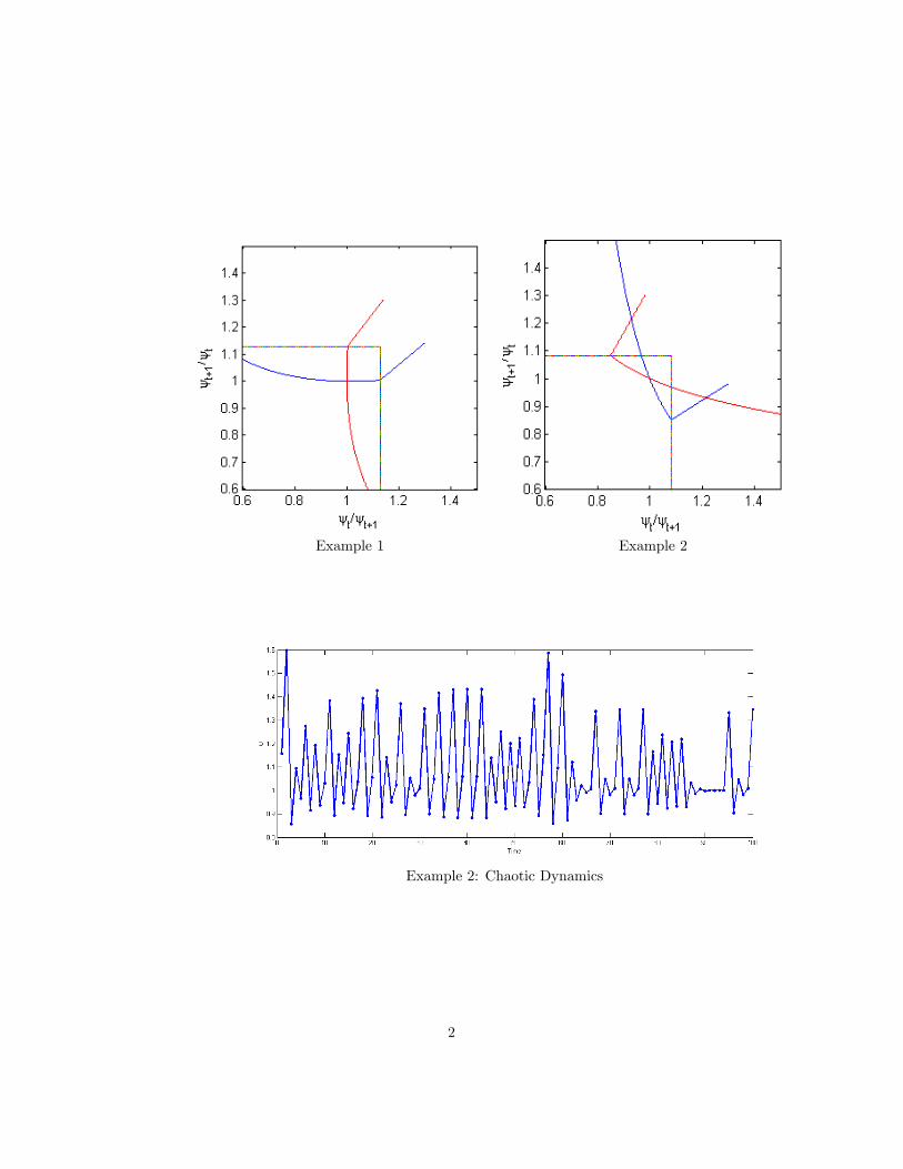
Example 1 Example 2

Example 2: Chaotic Dynamics

2

Example 3 Example 4

1 .4 1 .6 1 .8 2 2 .2 2 .4 2 .6 2 .8 30

0 .0 0 5

0 .0 1

0 .0 1 5

0 .0 2

0 .0 2 5

0 .0 3

0 .0 3 5

0 .0 4

H

Wel

fare

Example 5

3

�h = 0:5; � = 0:6; = 8; � = 3; � = 3:52; � = 1=3

4