How big is that cookie?The Integral Geometric approach togeometrical quantities

Abstract. Integral geometry studies the link between expectationof random variables and geometrical quantities like length, area orcurvature. This thesis focuses on how expectation of random vari-ables can be used to define reasonable notions of geometrical size.The simple idea of looking at the shadow when a compact convexbody in Rn is orthogonally projected onto a random k-dimensionalsubspace will generate a collection of “continuous invariant valua-tions”. A theorem of Hadwiger concludes that this collection spansthe vector space of all continuous invariant valuations, and thusintegral geometry elegantly provides a complete description aboutthe size of a compact convex body. Furthermore, some of thesevaluations turn out to be extensions of familiar geometrical con-cepts like surface area, but escape the typically required continuityor smoothness conditions and offer an alternative interpretation ofthese concepts.

In choosing a k-dimensional subspace at random, one needs tospecify a probability measure that is “invariant under the symme-tries of Euclidean space” so that the size of an object is unchangedafter it is displaced by a Euclidean motion. We explore the pos-sibility of imposing measures without such restrictions to obtainnew kinds of geometries, and perform this exploration on a genericsmooth manifold. Finally, we look at how a variant of the integralgeometric ideas explored permits the study of geometrical quanti-ties of a different flavor: various forms of curvature.

Harvard University 2015Barry Jia Hao Tng

Advisor:Oliver Knill

1

Acknowledgements

First, I would like to thank my family, especially my younger brother, for alwaysbeing supportive of me and cheering me on during difficult times. To my parents,I am proud to say that I have learnt a tremendous amount through my years inschool, and for that I have to thank you for your love and the environment youcreated for me.

Next, I would like to thank my advisor, Oliver Knill, for introducing me to thistopic that I had no prior exposure to but turned out to be an elegant and fascinatingarea of study. I thank him for all his patience in advising me and infecting me withall the enthusiasm he has for mathematics.

I have had the greatest fortune of being taught through the years by some ofthe most dedicated and amazing teachers, be it from Harvard or Raffles. I amdelighted to have learnt a great deal of mathematics from Sarah Koch, DennisGaitsgory, Curtis McMullen, Jacob Lurie, Alex Perry, Junecue Suh, Melody Chan,Sukhada Fadnavis, Siu Cheong Lau, Mark Kisin, and Shlomo Sternberg. I wouldalso like to thank Joe Blitzstein and David Morin for some of the most amazingcourses I have taken at Harvard.

Finally, I would like to thank my most precious friends who always stand by me- Zhang Wei, An, Chris, Diana and Dan. Each of you have a unique sense of humorthat never fails to cheer me up, and all of you have inspired me with your outlooksabout life. I would also like to thank Bang for helping me with the figures, andnumerous friends who offered to look over this thesis, especially Jeremy.

2

Contents

Acknowledgements 11. Introduction 31.1. Buffon and the Lens of Probability 31.2. Bertrand and Caution with Probability 51.3. Integral Geometry 81.4. Outline of Thesis 92. Invariant Measures 102.1. Theory of Lie Groups and Homogeneous Spaces 102.2. Grassmannians 132.3. k-planes 142.4. Example - Buffon’s Needle Problem in Rn 153. Notions of Size 183.1. “Reasonable” notion of size 183.2. Intrinsic Volumes 203.3. Hadwiger’s Theorem 223.4. Steiner’s formula 234. Lengths on Manifolds 294.1. From Needles to Noodles 304.2. Extension to Manifolds 305. Total Curvature Measures 345.1. Weyl’s Tube Formula 345.2. Local Steiner’s Formula 355.3. V -measures and Integral Geometry 376. Recent Developments 41References 43

1. Introduction

There is no royal road to geometry.– Euclid of Alexandria

In the 3rd Century BC, Euclid wrote one of the most influential textbooks ofall time – The Elements. In the treatise, Euclid revolutionized geometry by in-troducing an axiomatic approach. In the two millennia that have since passed,geometrical concepts like length, area and volume continue to be of relevance tothe human mind but have been subjected to much higher levels of abstraction andcomplexity in order to meet the standards of modern mathematics. For example,the definition of surface area can only be made for certain subsets of R3, such as asmooth surface, and may involve technical machineries such as parametrization andworking with integration of forms. Other geometrical concepts such as curvatureare only given rigorous definitions on a relatively recent timescale using the ab-stract setting of manifold theory and differential geometry, and also involve highlytechnical formulations.

Following the wise words of Euclid, one might gain new insights by exploring analternative road to understanding some of these geometrical quantities, especiallyin light of the high level of abstractions and technicalities involved in the definitions.

1.1. Buffon and the Lens of Probability. In 1733, the French mathematicianComte de Buffon first made the connection between probability theory and geom-etry with his famous Needle Problem (problem 1.1.1), opening the possibility ofusing a different approach to understanding geometry – using probability. Here is aquick recap of the problem and his solution published 4 years later, which will alsomake concrete what is meant by a possible probabilistic approach to understandinggeometry.

Problem 1.1.1. (Buffon’s Needle Problem) Let the xy-plane be ruled with parallellines of 1 unit apart – for concreteness, take the system of lines of the form y = mwhere m ∈ Z. Drop a needle (i.e. line segment with endpoints) of length l randomlyonto the plane. What is the probability that the needle will cross at least one of thelines? For the purpose of this discussion, we shall only consider the case 0 < l < 1,so that the needle can only cross at most one of the lines.

In formulating the problem, one needs to be mathematically precise about whatis meant by dropping the needle randomly onto the plane. To do this, note that itis sufficient to describe the position of the needle by a, the vertical distance betweenthe centre of needle to the closest line, and θ, the acute angle formed by the needleand the vertical direction. We shall reasonably choose these random variables toindependently follow a uniform distribution, specifically:

a ∼ Unif [0, 1/2] and θ ∼ Unif [0, π/2]

4

1

1

al

2cos θ

θ

a l

2cos θθ

Figure 1.1.

This means that the joint probability density function of (a, θ) is4/π 0 ≤ a ≤ 1/2 and 0 ≤ θ ≤ π/20 otherwise

Solution. A simple geometric analysis (figure 1.1) shows that the needle crosses aline if and only if

a ≤ l

2cos θ

The probability that our random variables satisfy the above inequality is given by∫ π2

0

∫ l2 cos θ

0

4

πda dθ =

2l

π

This solves the Buffon’s Needle Problem (at least for 0 < l < 1).

There is an alternative interpretation of the above result. Let X be the randomvariable denoting the number of intersections between the needle and the systemof lines. In our case of 0 < l < 1, X can only take two possible values, 0 or 1. Thismeans that E[X] is the probability that the needle intersects some line. Therefore1,

(1.1) E[X] =2l

π

It is easy to show that equation (1.1) holds for all l > 0. Namely, mentallyconsider the needle to be composed to shorter needles of length l1, . . . , ln piecedtogether2, where 0 < li < 1 and l1 + · · · + ln = l. Define Xi to be the numberof intersections between the ith piece and the system of lines, which means X =

1Note that this result holds even if our needle does not have one or both its endpoints included.2The careful reader would worry about what happens at the gluing points between two short

needle pieces, since they appear to be counted twice. However, by the previous footnote, we canensure that each point of a long needle is only counted once by disregarding, where necessary, oneor more endpoints of our short needle pieces.

5

X1 + · · · + Xn. Now, linearity of expectations holds regardless of the dependencybetween the Xi’s, so3

E [X] = E

[n∑i=1

Xi

]=

n∑i=1

E [Xi] =

n∑i=1

2liπ

=2l

π

This is a remarkable result. It states that the length of a needle can be computed(up to a scaling factor of π/2) by looking at the average number of intersections withthe system of lines. This is a glimpse of how the expectation of a random variablecan be used to calculate a geometrical quantity. We shall need this relation later,so let us record our discussion down as a proposition.

Proposition 1.1.2. Under the set-up of problem 1.1.1 (and the accompanyingdefinition of “random”), the expected number of intersections between the needleand the system of lines is given by 2l/π.

1.2. Bertrand and Caution with Probability. A key decision made in formu-lating the Buffon’s Needle Problem was how to place the needle randomly. Theinfamous Bertrand’s paradox tells us that this is not a decision that can be ig-nored. Although the paradox will not be discussed in detail here (see [Tis84]), itsuffices to say that Bertrand exhibited the possibility of obtaining different answersto probability questions if the phrase “at random” can be interpreted in differentways. In our context, if we had chosen a different definition of placing our needlerandomly, then E [X] would turn out to be different, and may in fact be unrelated(or related in a complicated way) to l. We were fortunate that the most intuitivechoice made above turns out to give not just a relation between E [X] and l, butin fact the relation is linear (i.e. simple!). How might one choose the probabilitymeasure to ensure that there is a relation between E [X] and l?

To get a sense of what additional properties our probability measure shouldhave, consider the Buffon’s Needle Problem generalized to 3 dimensions. Here,there are a system of parallel planes spaced 1 unit apart and a needle of lengthl. Previously, as a matter of respecting the convention of the original problem, wefixed the system of lines and placed the needle randomly. From this point on, itwill be more useful to think that there is a needle fixed in space whose length weare interested in measuring, and we are doing this by randomly imposing a systemof parallel planes and computing the expected number of intersections, which wewill denote by E [X]. In other words, we get to choose the probability measure onsystems of planes and want a relation between E [X] and l that is true no matterhow the needle has been fixed in space.

Suppose temporarily that we always fix our needle to be parallel to the z-axisof our xyz-space, with its middle at the origin. Here is a perfectly legitimateprobability measure to impose on our system of planes that will turn out to givea linear relation between E [X] and l in this temporary set-up, but will later beshown to actually be lacking. A system of planes is determined once we picked(θ, φ, a), where the polar angle θ and azimuth angle φ determines a direction inspace for which the planes will be perpendicular to, and a is the closest distance of

3Before we can apply the result E [Xi] = 2li/π, we have to show that the position of the ith

piece has been placed in accordance to the (a, θ) distribution described above. Technically weonly know this for the entire needle, but it is straightforward to see that this implies the same for

the ith piece.

6

θ

φ

x

y

z

a

Figure 1.2.

the origin to a plane in the system (see figure 1.2). We set

θ ∼ Unif [0, π] , φ ∼ Unif [0, 2π] , a ∼ Unif [0, 1/2]

with these three random variables being independent.If 0 < l < 1, then a similar geometric analysis tells us that the needle crosses

a plane if and only if the needle, when projected onto the line normal to all theplanes, crosses a plane. This happens if and only if

a ≤ l

2|cos θ|

See figure 1.3. The probability that our random variables satisfy the above inequal-ity is given by ∫ 2π

0

∫ π

0

∫ l2 |cos θ|

0

2 · 1

π· 1

2πda dθ dφ =

2l

π

By a similar reasoning to those leading up to theorem 1.1.2, we see that for alll > 0, we have E [X] = 2l/π. There is indeed a linear relation between E [X] and l.

However, in general, the needle is simply fixed in space, pointing in an arbitrarydirection at an arbitrary position. We want to use a single probability measure onour system of planes to compute the length of any fixed needle. Unfortunately, theformula E [X] = 2l/π is no longer always true. For example, if the fixed needle

7

x

y

z

l

2

| θl

2cos |

a

Figure 1.3.

is pointing along the x-direction with its middle at the origin, then by the sameprojection argument a needle of length l < 1 crosses a plane if and only if

a ≤ l

2sin θ|cosφ|

The probability that our random variables satisfy the above inequality is given by∫ 2π

0

∫ π

0

∫ l2 sin θ|cosφ|

0

2 · 1

π· 1

2πda dθ dφ =

4l

π2

This time, we have E [X] = 4l/π2 6= 2l/π.In summary, the probability measure that was imposed failed to give any relation

between E [X] and l, beause E [X] also depends on other parameters of the needle(e.g. its direction). There is actually a linear relation if we restrict the needles toalways be lying along a certain direction in space, but this is a silly restriction. Ifonly the probability measure is somehow compatible with rotation, then a singlerelation holding for needles along one direction will also hold for all needles ingeneral. This motivates the following definition.

Definition 1.2.1. Suppose T is a set equipped with a group action by G. For asubset S ⊆ T and an element g ∈ G, we write gS := gt | t ∈ S. The measure µof a measure space (T,Σ, µ) is said to be G-invariant (or simply invariant) if forall S ∈ Σ, we have gS ∈ Σ and µ (S) = µ (gS).

8

The set T containing all possible systems of planes is equipped with the actionby the Euclidean group E(3). The preceding discussion motivates why any measurewe consider imposing on T should preferably be E(3)-invariant (and Σ should befine enough so that X : T → R ∪ ±∞ is a random variable4, i.e. measurable5).Specifically, if for a particular fixed needle we find E [X] to be of a certain value,then we can subject the needle to any Euclidean motion and its length is notgoing to change under Euclidean motion, so E [X] had better be unchanged if wewant a relation between E [X] and l. Choosing a E(3)-invariant measure on Twill guarantee this. Of course, the relation may not be linear, but it is a relationnonetheless. We will finish up this discussion of the Buffon’s Needle Problem oncewe have more tools (example 2.4.1).

1.3. Integral Geometry. In the late 1930s, Wilhelm Blaschke published a seriesof papers under the project “integral geometry”. His idea was to investigate, aswe have tried above, whether expectations of random variables could be used forcalculating and understanding geometrical quantities like length, area or curvature.Morgan Crofton, in the late 1800s, actually preceded this effort with the discovery ofmany simple relations of this flavor. However, his work and even simply the idea ofusing probability to study geometrical quantities, which went by the umbrella title“geometric probability”, came under great threat of being completely discreditedafter the paradox of Bertrand attacked Crofton’s loose treatment of randomness.With no unified or consistent approach to value one definition of randomness overanother, the theory appears highly arbitrary as to when a definition will lead to arelation. It was Poincare who, in 1896, kept the idea alive by suggesting that theonly definitions of randomness worth considering be limited to measures that areinvariant under any symmetry group which the interested geometrical quantity isknown to be invariant under. He coined the term “kinematic density” for what ismore commonly called an invariant measure today.

Having been revived by the rebranding of Blaschke, the field has made notewor-thy progress in the past half a century. The most important is probably establishingthe use of homogeneous space theory as a unified approach to obtain the measureof interest, a work done by two of Blaschke’s students, Andre Weil and Shiing-ShenChern. Integral geometry offers itself as an interesting alternative tool to study ge-ometrical problems (for example, Milnor [Mil50, 3.1] used this to study curvature ofknots), but is also used today in stochastic geometry [SW08], computational model-ing (for example, tomography) [KW03] and even made an appearance in statisticalphysics [Mec98].

The name “integral geometry” deserves a brief comment. The goal of the field isto link geometry with expectation of random variables, which is actually an integralof the random variable as a measurable function over the probability space, hencethe name. In some cases, it is neater to not limit ourselves to probability spaces.Throughout, we will abuse terminology and also use the term “expectation” of ameasurable function to denote its integral over the measure space.

4We considered the extended real numbers because the needle could very well lie in one of the

planes, in which case the number of intersections is ∞. We might be tempted to disregard thissituation by saying that it occurs with zero measure, but recall that we have yet to define our

measure on T , so the phrase ”zero measure” makes no sense.5The Borel σ-algebra of the extended real numbers consists of all sets S for which S ∩ R is a

Borel set in the usual sense.

9

1.4. Outline of Thesis. Integral geometry is a rich field with its tentacles span-ning into many areas of mathematics. This thesis will choose to focus on howexpectations can be used to define reasonable notions of geometric sizes. For ex-ample, the “surface area” of a solid in R3 might be considered a reasonable notionof size. However, we remarked earlier that a formal definition by conventionalmethods only assigns surface area to certain subsets of space and involves certaintechnical machineries to set-up fully. Using the idea of expectations, we will – ina single breath – cleanly define an entire collection of notions of geometric size,one of which will be reminiscence of surface area (we will, for example, realize thatthere is agreement for convex polyhedrons), defined even for some subsets of R3 forwhich the conventional approach does not ascribe a surface area. A theorem dueto Hadwiger will tell us why the single breath we took was enough to understandall reasonable notions of geometric sizes. This discussion will be done in chapter 3and is the center point of the thesis.

Chapter 2 carries out the preparatory work of establishing certain invariantmeasures that we will need. In particular, for 0 ≤ k ≤ n, the GrassmannianGr(n, k) := k dimensional subspaces of Rn is acted upon by the orthogonalgroup O(n) and the set of all k-planes Aff(n, k) is acted upon by the Euclideangroup E(n); we will need invariant measures for both. To do this, we will use thetheory of homogeneous spaces and treat O(n) and E(n) as Lie groups.

Chapters 4 and 5 are bonus sections where we extend particular ideas presentedin chapter 3. Treatment in these two chapters is designed to give a flavor of thepower of integral geometry beyond this thesis.

In chapter 4, we present some original ideas and pursue the thread of usingintegral geometry to define the notion of length, but extended to curves on arbitrarysmooth manifolds. The chapter will allow us to better appreciate how integralgeometry can be used as the starting point for prescribing geometries, assigningdistance functions to a smooth manifold with no presupposed geometry.

In chapter 5, we discuss how the integral geometric framework can also encom-pass the different geometrical notion of curvature.

2. Invariant Measures

In these days the angel of topology and the devil of abstract algebra fightfor the soul of every individual discipline of mathematics.

– Hermann Weyl

As we have seen, one of the key prerequisites to integral geometry is the studyof invariant measures. In this chapter, we recap some of the main takeaways fromthe theory of homogeneous spaces that will be useful for integral geometry. Inparticular, we will establish the existence of invariant measures for a wide class ofcontexts that are frequently useful for practical applications in integral geometry.We will also pay particular attention to the examples of Grassmannians and theset of k-planes in Rn.

For this purpose, we will be needing some standard material from smooth man-ifold theory, which we will be prepared to cite as long as it is discussed in [Lee12],a standard textbook on the subject.

2.1. Theory of Lie Groups and Homogeneous Spaces. In definition 1.2.1, weare under the most general context where there is simply a set T equipped witha group action by G. In most applications, G can have an additional structure ofa Lie group, which will turn out to be a huge resource. Recall that a Lie groupG is a group whose elements are also points of a smooth manifold, such that thegroup operation (g, h) 7→ gh and inversion map g 7→ g−1 are both smooth. Thereare two examples of Lie groups that will be relevant to our purpose. They arethe orthogonal group O(n), which is the set of n × n real matrices A satisfyingATA = AAT = I, and the Euclidean group E(n), which is the symmetry group ofn-dimensional Euclidean space (i.e. in particular including the translation groupT (n) and O(n) as subgroups). For a proof that these are Lie groups, see [Lee12,7.27] and [Lee12, 7.32].

Let us first study the situation of a Lie group G acting on by itself via leftmultiplication and see if we can obtain an invariant Borel measure on G (in thesense of definition 1.2.1). Note that here we chose the σ-algebra of the measurespace to be Σ = B(G), where the notation B(X) will be used to denote the Borelσ-algebra of X whenever X is a topological space.

Indeed, we have the following useful starting point from smooth manifold theory.

Theorem 2.1.1. Every Lie group, which can always be endowed with a left-invariant orientation, has a nowhere-vanishing positively-oriented left-invariant (con-tinuous) n-form (where n = dimG). Moreover, all left-invariant n-forms are equal,up to constant multiples.

Proof. See [Lee12, 16.10].

Theorem 2.1.2. Let G be a Lie group acting on itself by left multiplication. Thenthere is a measure µ on (G,B(G)) such that µ is invariant.

11

Before proceeding with the proof, we need a few pieces of notation. We let Cc(G)denote the space of continuous functions on G with compact support. If U is anopen set in G and f ∈ Cc(G), we use the notation

f ≺ Uto mean 0 ≤ f ≤ 1 and supp(f) ⊆ U . Also observe that if f ∈ Cc(G) and ω isa (continuous) n-form, then fω is a compactly supported (continuous) n-form, so∫Gfω makes sense (after we chose an orientation for G).

Proof. Endow G with a left-invariant orientation and let ω denote a nowhere-vanishing positively-oriented left-invariant (continuous) n-form.

Step 1: Let us first construct a candidate Borel measure. We define, for U ⊆ Gopen,

µ0(U) := sup

∫G

fω | f ∈ Cc(G), f ≺ U

and for an arbitrary E ⊆ G, we define

µ∗ (E) := inf µ0(U) | U ⊇ E, U openObserve that µ0(U) ≤ µ0(V ) if U ⊆ V and so µ∗(U) = µ0(U) for U open. Let usshow that µ∗ is an outer measure. For that, we need this lemma.

Lemma: If U1, U2, . . . is a sequence of open sets and U :=⋃∞j=1 Uj , then

µ0(U) ≤∑∞j=1 µ0(Uj).

Proof of Lemma: Let f ∈ Cc(G) be such that f ≺ U . By compactness of

supp(f), we can pick N such that supp(f) ⊆ ⋃Nj=1 Uj . Since⋃Nj=1 Uj is a smooth

manifold, by the Existence of Partitions of Unity theorem [Lee12, 2.23], we can find

smooth functions g1, . . . , gN :⋃Nj=1 Uj → R such that gj ≺ Uj and

∑Nj=1 gj ≡ 1 on⋃N

j=1 Uj . Then f =∑Nj=1 fgj and fgj ≺ Uj , so∫

G

fω =

n∑j=1

∫G

fgjω ≤n∑j=1

µ0(Uj) ≤∞∑j=1

µ0(Uj)

and therefore by definition of µ0, we conclude that µ0(U) ≤∑∞j=1 µ0(Uj).

As a consequence of the lemma and basic measure theory (e.g. [Fol99, 1.10]),we learn that µ∗ is an outer measure. Now, we show that every open set is µ∗-measurable, that is, let U be open and we want to show that whenever E ⊆ X issuch that µ∗(E) <∞, we will have µ∗(E) ≥ µ∗(E ∩ U) + µ∗(E ∩ U c). Fix ε > 0.

If E happens to be open, then we can find f1 ∈ Cc(G) with f1 ≺ E ∩ U suchthat

∫Gf1ω > µ0(E ∩U)− ε, and similarly find f2 ∈ Cc(G) with f2 ≺ E− supp(f1)

such that∫Gf2ω > µ0(E − supp(f1))− ε. Note f1 + f2 ≺ E and so

µ∗(E) = µ0(E) ≥∫G

(f1 + f2) ω > µ0(E ∩ U) + µ0(E − supp(f1))− 2ε

= µ∗(E ∩ U) + µ∗(E − supp(f1))− 2ε ≥ µ∗(E ∩ U) + µ∗(E ∩ U c)− 2ε

For E not necessarily open, we find open V such that V ⊇ E and µ∗(V ) = µ0(V ) <µ∗(E) + ε. Then

µ∗(E) + ε > µ∗(V ) ≥ µ∗(V ∩ U) + µ∗(V ∩ U c) ≥ µ∗(E ∩ U) + µ∗(E ∩ U c)and so the desired inequality also holds.

12

Therefore, the collection of µ∗-measurable sets will contain B(G), and we candefine µ := µ∗|B(G) as a Borel measure.

Step 2: We check that µ is invariant. Let E ∈ B(G) and g ∈ G. Note that leftmultiplication by g is a homeomorphism, so gE ∈ B(G). By definition,

µ (gE) = inf µ0(U) | U ⊇ gE,U open = inf µ0(gU) | U ⊇ E,U openBut

µ0(gU) = sup

∫G

fω | f ∈ Cc(G), f ≺ gU

= sup

∫G

f(L∗g−1ω) | f ∈ Cc(G), f ≺ U

= µ0(U)

where L∗g−1 denotes the pullback by the diffeomorphism Lg−1 that is left multi-

plication by g−1, and where we used the left-invariance of ω in the last equality.Therefore µ(gE) = µ(E) as desired.

As a step towards increasing generality, let G be a Lie group and H a closedsubgroup of G. The left coset space G/H can be equipped with a smooth manifoldstructure such that the quotient map π : G→ G/H is smooth [Lee12, 21.17]. Underthis structure, G/H can be acted on by G via

g1g2 = g1g2

and this action is smooth.

Proposition 2.1.3. There is an invariant Borel measure for G/H equipped withthe above action by G.

Proof. Equip G with the invariant Borel measure µ. G/H here is equipped withthe Borel σ-algebra. The map π : G→ G/H is smooth, thus continuous, and hencemeasurable. Therefore, the pushforward measure π∗(µ) is a Borel measure on G/H.It is invariant because for S ∈ B(G/H), we have gS ∈ B(G/H) because the actionof g on G/H is a homeomorphism, and

(π∗(µ))(gS) = µ(π−1(gS)) = µ(g(π−1(S))) = µ(π−1(S)) = (π∗(µ))(S)

as desired.

The above consideration involving G/H is actually a lot more general than itmight first appear. A homogeneous G-space (or simply homogeneous space)is a smooth manifold endowed with a transitive smooth action by the Lie groupG. Clearly, G/H is an example of a homogeneous G-space. The following theoremtells us that in fact all homogeneous spaces look like this.

Theorem 2.1.4. Let G be a Lie group and M a homogeneous G-space. Pick anypoint p ∈ M . Then the stabilizer of p, denoted Stab(p) is a closed subgroup of Gand the map F : G/Stab(p)→M defined by F (g) = gp is a diffeomorphism.

Proof. See [Lee12, 21.28].

Corollary 2.1.5. A homogeneous G-space can be equipped with an invariant Borelmeasure.

Proof. Pick any p ∈M and consider the pushforward of the invariant Borel measureof G/Stab(p) using the map F as defined in theorem 2.1.4.

13

Finally, the following theorem is useful if we start with a set that might not yetbe equipped with a smooth manifold structure.

Theorem 2.1.6. Let T be a set, endowed with a transitive action by a Lie groupG such that for some p ∈ T , we know that the stabilizer subgroup Stab(p) is closedin G. Then T can be made into a smooth manifold such that it is a homogeneousG-space.

Proof. See [Lee12, 21.20].

2.2. Grassmannians. The above discussion can be applied to two examples ofparticular interest to integral geometry. The first is Gr(n, k), the set of all k-dimensional subspaces of Rn, acted transitively upon by O(n) (k here is some fixedinteger satisfying 0 ≤ k ≤ n). If we arbitrarily pick an element L0 ∈ Gr(n, k), thenStab(L0) is some copy of O(k)×O(n− k) inside O(n) which can be shown to be aclosed subgroup. For example, if we view O(n) as the set of n×n orthogonal matri-ces with respect to the standard basis (ε1, . . . , εn) and select L0 = span(ε1, . . . , εk),then Stab(L0) is the set of matrices of the form(

A 00 D

)where A andD are orthogonal matrices of sizes k×k and (n−k)×(n−k) respectively.We shall abuse notation and understand O(k)×O(n− k) as a specific subgroup ofO(n). The smooth manifold structure (which includes the topology) of Gr(n, k) isthen better understood as

Gr(n, k) ' O(n)

O(k)×O(n− k)

and has an O(n)-invariant Borel measure.Let θn denote a O(n)-invariant Borel measure on O(n) itself, which exists by the-

orem 2.1.2. The corresponding O(n)-invariant Borel measure on Gr(n, k), denoted6

by γn,k, is obtained by (two) pushforwards and concretely is given by

γn,k (A) = θn(g ∈ O(n) | gL0 ∈ A)

for any A ∈ B(Gr(n, k)).In turn, here is one way of defining some θn that is practical for our applica-

tions. Observe that there is a bijection between elements of O(n) and an orderedorthonormal basis under the map g 7→ (e1, . . . , en) = (g(ε1), . . . , g(εn)). We beginby picking e1 ∈ Sn−1 in accordance to the normalized spherical measure σn−1 (nor-malized means σn−1(Sn−1) = 1). Now, e2 must be picked from the copy of Sn−2

that lies in the hyperplane orthogonal to e1, and we pick e2 in accordance to thenormalized spherical measure σn−2. In general, we pick ei uniformly from the copyof Sn−i that lies in the (n− i+ 1)-dimensional plane orthogonal to e1, . . . , ei−1. In

6We chose the symbol γ because “gamma” and “Grassmannians” both start with “g”. Likewise,hopefully the symbol θ reminds one of angles and thus serves as a mnemonic for the measure on

O(n).

14

other words, we can define θnvia∫O(n)

f(g) θn(dg)

=

∫Sn−1

∫Sn−2⊥e1

. . .

∫S0⊥e1,...,en−1

f(εi 7→ ei) σ0(den) . . . σn−2(de2) σn−1(de1)

for any measurable function f (and εi 7→ ei denotes the unique element of O(n)that maps εi to ei).

From the above description of θn, we have γn,k(Gr(n, k)) = θn(O(n)) = 1, sofor each fixed n and k, Gr(n, k) is already a probability space. No normalization isneeded.

We will need the following lemma in the future.

Lemma 2.2.1. Let f be a measurable function on Gr(n, k). Then∫Gr(n,k)

f(L) γn,k(dL) =

∫Gr(n,n−k)

f(L⊥) γn,n−k(dL)

Proof. Pick any L0 ∈ Gr(n, k). For a subset A ⊆ Gr(n, k), we let A⊥ ⊆ Gr(n, n−k)denote

A⊥ :=L⊥ | L ∈ A

Observe that

γn,k(A) = θn(g ∈ O(n) | gL0 ∈ A) = θn(g ∈ O(n) | gL⊥0 ∈ A⊥

) = γn,n−k(A⊥)

from which the desired conclusion follows.

2.3. k-planes. A similar discussion can be made for Aff(n, k), the set of all k-dimensional planes in Rn, acted upon transitively by E(n). Recall that E(n) canbe written as the semi-direct product T (n) o O(n), where T (n) is the translationgroup and O(n) acts on T (n) ' Rn in the usual way (for a review of Lie groupstructure under semi-direct products, see [Lee12, 7.32]). As a matrix group, E(n)can be realized as matrices of the form

A11 . . . A1n b1...

. . ....

...An1 . . . Ann bn

0 . . . 0 1

where A is an orthogonal matrix (standard basis chosen here) and b is a vector(again, standard basis). Pick an element P0 ∈ Aff(n, k). Then Stab(P0) is somecopy of (T (k)×e)o(O(k)×O(n−k)) inside E(n) which can be shown to be a closedsubgroup. For example, without loss of generality, suppose P0 = span(ε1, . . . , εk).Then Stab(P0) consists of matrices of the form A′ 0 b

0 A′′ 00 0 1

where A′ is orthogonal of size k× k, A′′ is orthogonal of size (n− k)× (n− k) andb is a vector of length k. We will abuse notation and understand (T (k) × e) o(O(k)×O(n− k)) as a subgroup of E(n). Then, as smooth manifolds,

Aff(n, k) ' E(n)

(T (k)× e) o (O(k)×O(n− k))

15

and has an invariant Borel measure.There is a natural candidate for an invariant Borel measure on E(n). First, we

perform a verification that B(E(n)) = B(T (n)) ⊗ B(O(n)). Indeed, the smoothmanifold structure of semi-direct product is taken to be that of the Cartesian prod-uct, in which case the topology is the product topology. Now T (n) and O(n) areLie groups, hence second-countable and thus separable; they are also metrizable

(they inherit the metric from Rn and Rn2

respectively). The result follows fromthis standard lemma from measure theory.

Lemma 2.3.1. If X1, . . . , XN are metric spaces and X is∏Nj=1Xj equipped with

the product topology, then⊗N

j=1B(Xj) ⊆ B(X). If furthermore X1, . . . , XN are

separable, then⊗N

j=1B(Xj) = B(X).

Proof. See any text in measure theory, for example [Fol99, 1.5].

Let λn denote the n-dimensional Lebesgue measure, which we restrict to Borelsets but continue to use the same symbol as a mild abuse of notation, and recall θnfrom section 2.2. Since we have B(E(n)) = B(T (n))⊗B(O(n)), it makes sense forus to talk about the product measure λn×θn as a Borel measure on E(n). One cancheck that this is an E(n)-invariant measure. Under the pushforwards, we obtainan E(n)-invariant measure on Aff(n, k), which we denote7 by αn,k.

One can work through the details of the pushforwards and obtain the followingpractical interpretation of αn,k: choosing a k-plane can be seen as choosing anelement of Gr(n, k) in accordance to γn,k and then translating the subspace along adirection in its orthogonal complement chosen in accordance to λk. In other words,we can understand αn,k as∫

Aff(n,k)

f(P ) αn,k(dP ) =

∫Gr(n,k)

∫L⊥

f(L+ y) λk(dy) γn,k(dL)

for any measurable function f .

2.4. Example - Buffon’s Needle Problem in Rn. As a nice opportunity toillustrate the ideas of this chapter, let us finish off the Buffon’s Needle Problemthat was unsettled in the introduction.

Example 2.4.1 (Buffon’s Needle Problem in Rn). Let there be a needle of lengthl fixed in Rn, n ≥ 2. We have to choose a probability measure on systems ofparallel hyperplanes spaced a unit apart, and hopefully obtain a relation betweenthe expected number of intersections and l.

We have already discussed that because the needle length is invariant underE(n), we had better choose a probability measure that is E(n)-invariant. The setT containing all systems of hyperplanes is equipped with the action by E(n), andvery similar to the discussion of k-planes, we can obtain an E(n)-invariant Borelmeasure αn,n−1 where∫

T

f(P ) αn,n−1(dP ) =

∫Gr(n,n−1)

∫ 1

0

f(L+ y) λ1(dy) γn,n−1(dL)

for any measurable function f . The inner integral ranges from 0 to 1 becausetranslating the system of hyperplanes along the normal direction will lead to the

7Again, “lambda” and “Lebesgue” both start with the same letter, as do “alpha” and “affine”.

16

same configuration every integer distance. Note that αn,n−1 is already normalizedto be a probability measure because take f(P ) ≡ 1 and we get

αn,n−1(T ) = λ1([0, 1]) · γn,n−1(Gr(n, n− 1)) = 1

Let X : T → R∪±∞ denote the number of intersections, which can be shownto be a random variable, i.e. measurable. First assume 0 < l < 1. Then

E [X] =

∫T

X(P ) αn,n−1(dP )

=

∫Gr(n,n−1)

∫ 1

0

X(L+ y) λ1(dy) γn,n−1(dL)

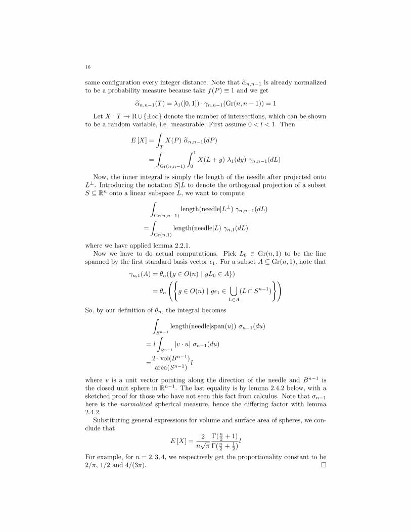
Now, the inner integral is simply the length of the needle after projected ontoL⊥. Introducing the notation S|L to denote the orthogonal projection of a subsetS ⊆ Rn onto a linear subspace L, we want to compute∫

Gr(n,n−1)

length(needle|L⊥) γn,n−1(dL)

=

∫Gr(n,1)

length(needle|L) γn,1(dL)

where we have applied lemma 2.2.1.Now we have to do actual computations. Pick L0 ∈ Gr(n, 1) to be the line

spanned by the first standard basis vector ε1. For a subset A ⊆ Gr(n, 1), note that

γn,1(A) = θn(g ∈ O(n) | gL0 ∈ A)

= θn

(g ∈ O(n) | gε1 ∈

⋃L∈A

(L ∩ Sn−1)

)So, by our definition of θn, the integral becomes∫

Sn−1

length(needle|span(u)) σn−1(du)

= l

∫Sn−1

|v · u| σn−1(du)

=2 · vol(Bn−1)

area(Sn−1)l

where v is a unit vector pointing along the direction of the needle and Bn−1 isthe closed unit sphere in Rn−1. The last equality is by lemma 2.4.2 below, with asketched proof for those who have not seen this fact from calculus. Note that σn−1

here is the normalized spherical measure, hence the differing factor with lemma2.4.2.

Substituting general expressions for volume and surface area of spheres, we con-clude that

E [X] =2

n√π

Γ(n2 + 1)

Γ(n2 + 12 )l

For example, for n = 2, 3, 4, we respectively get the proportionality constant to be2/π, 1/2 and 4/(3π).

17

Lemma 2.4.2. Let v be a fixed unit vector. Then∫Sn−1

|v · n| dS = 2 · vol(Bn−1)

where dS is the usual surface element and n is the outward unit normal vector.

Proof. (Sketch) A full proof can be found in [KR97, 5.5.1]. Chop up the surfaceinto many small regions Ai with surface area S(Ai) and we have the approximation∫

Sn−1

|v · n| dS ≈∑i

|v · ni| S(Ai)

Observe that |v · ni| S(Ai) is approximately the area of the shadow when Ai isorthogonally projected onto the hyperplane v⊥. On orthogonal projection, eachhemisphere as separated by v⊥ covers the solid unit ball in v⊥ once. Thus theabove sum is approximately equal to 2 · vol(Bn−1). The approximations becomeequality in the limit.

3. Notions of Size

Mathematics is the art of giving the same name to different things.– Henri Poincare

We are ready to see how expectations can be used to define reasonable notionsof size. Actually the Buffon’s Needle Problem of example 2.4.1 gave us a glimpseof this idea – the length of a needle can be computed (up to scaling factor) as theexpectation of a random variable. However, the example is not very satisfactoryon two accounts: the length of a line segment is not a difficult concept to grapplewith, and we want to avoid having to search from scratch a random variable foreach reasonable notion of size that one can think of. Fortunately, this chapter willexplain how integral geometry provides an elegant and unified way to think aboutall reasonable notions of size, many of which are difficult to grasp by classicalapproaches.

As the Banach-Tarski paradox shows, attempting to assign sizes to every subsetof Rn is a tricky business. Our theory will focus only on Kn, the collection ofall compact convex subsets of Rn. This collection is wide enough to include someexamples of smooth manifold (or rather, the boundary of the subset is a smoothmanifold), polyhedrons, but also other less well-behaved examples. Yet, it is narrowenough to produce an elegant theory. We shall also remark that once we completeda discussion for Kn, it is possible to extend our size functions to the collection ofpolyconvex sets (i.e. the collection consisting of finite unions of compact convexsets) by a direct application of an extension theorem by Groemer. However, we willnot pursue this discussion here – a good reference on Groemer’s extension theoremwill be [KR97, Chapter2]. The collection of polyconvex sets practically covers allgeometrical objects one would deal with in real life8; even this ‘o’ is really a finiteunion of convex pixels9. We merely wish to point out that the generality of thistheory, though limited to Kn, is not something to be underestimated.

3.1. “Reasonable” notion of size. A notion of size will be a map φ : Kn → R,but we should not allow every possible such mapping. There will be some propertieswe hope φ should satisfy before it will be convincing to call φ a notion of size. Below,three such properties are described.

Definition 3.1.1. The map φ : Kn → R is said to be a valuation if φ(∅) = 0 and

φ(K ∪ L) = φ(K) + φ(L)− φ(K ∩ L)

whenever K,L ∈ Kn are such that K ∪ L ∈ Kn.

Definition 3.1.2. The map φ : Kn → R is said to be invariant if φ(gK) = φ(K)for all K ∈ Kn and g ∈ E(n), where gK := g(x)|x ∈ K.

8That said, I am not completely sure what mathematicians will regard as “real life”.9In some sense, everything we encounter in real life is a finite union of atoms, but I will leave

it to the physicists to decide if we are permitted to talk about atoms as “convex”.

19

We will want φ to be an invariant valuation. Before describing the third property,it will be useful to recall what is known as the Hausdorff metric.

Definition 3.1.3. For K,L ∈ Kn, define the Hausdorff distance between themto be

δ(K,L) := max

supk∈K

d(k, L), supl∈L

d(K, l)

= max

supk∈K

infl∈L

d(k, l), supl∈L

infk∈K

d(k, l)

where d refers to the Euclidean metric in Rn.

Note that δ is not yet shown to be a metric. Before doing that, here is a lemmathat provides a more intuitive way of understanding δ. The statement of the lemmarequires us to first understand the ε-fattening of an object in Kn, where ε ≥ 0. Wedefine the ε-fattening of ∅ to be ∅, and for non-empty K ∈ Kn,

K+ε := x ∈ Rn | d(K,x) ≤ εRecall that for K,L ∈ Kn, their Minkowski sum is given by

K + L := k + l | k ∈ K, l ∈ LThus, we can also write K+ε = K + εBn, where εBn is the solid unit sphere ofradius ε. Note that K+ε is bounded, closed (from continuity of d(K, ·)) and convex(given x, y ∈ K+ε, decompose x, y using the Minkowski sum and then use the factthat both K and εBn are convex), whence K+ε ∈ Kn.

Lemma 3.1.4. Let K,L ∈ Kn. Then δ(K,L) ≤ ε if and only if K ⊆ L+ε andL ⊆ K+ε. Hence, we may equivalently define

δ(K,L) = inf ε ≥ 0 | K ⊆ L+ε and L ⊆ K+εand in fact, the above infimum is achieved.

Proof. If L ⊆ K+ε, then every l ∈ L obeys d(K, l) ≤ ε. Similarly if K ⊆ L+ε, thenevery k ∈ K obeys d(k, L) ≤ ε. Therefore,

δ(K,L) = max

supk∈K

d(k, L), supl∈L

d(K, l)

≤ ε

Conversely, we prove the contrapositive. WLOG suppose L ⊆ K+ε is violated, so

there exists l ∈ L such that d(K, l) > ε. Then δ(K,L) ≥ d(K, l) > ε.Note that if K ⊆ L+ε and L ⊆ K+ε hold, then K ⊆ L+η and L ⊆ K+η also hold

for any η > ε. Thus

E := ε ≥ 0 | K ⊆ L+ε and L ⊆ K+εis either of the form (c,∞) or [c,∞) for some c ≥ 0. By the first half of the lemma,δ(K,L) cannot be bigger or smaller than c, so δ(K,L) = c. Then again by the firsthalf of the lemma, c ∈ E so E = [c,∞) and the infimum is achieved.

Proposition 3.1.5. The Hausdorff distance δ is a metric and turns Kn into ametric space.

Proof. First, δ maps into R because our sets are compact (in particular bounded).δ is clearly symmetric, non-negative, and δ(K,K) = 0 for K ∈ Kn. If K,L ∈ Kn

are distinct, at least one of K −L or L−K will be non-empty; WLOG say we canpick some l ∈ L−K. Since K is compact (in particular closed), d(K, l) > 0. Thus

δ(K,L) ≥ d(K, l) > 0.

20

It remains to prove the triangle inequality. Let K,L,M ∈ Kn and ε = δ(K,M),η = δ(L,M). By lemma 3.1.4,

K ⊆M+ε and M ⊆ L+η

and so K ⊆ L+(ε+η) and similarly L ⊆ K+(ε+η). Again by lemma 3.1.4, δ(K,L) ≤ε+ η.

Now we may state the final property that φ should have.

Definition 3.1.6. The map φ : Kn → R is simply said to be continuous if it is acontinuous map with the Hausdorff metric on Kn and the usual Euclidean metricon R.

In summary, we shall be interested in studying the collection of all continuousinvariant valuations on Kn, which we shall denote Valn. Here is an easy propertyof Valn that already provides a lot of information about its structure.

Proposition 3.1.7. Valn is a real vector space under the usual definition of howto add functions and perform scalar multiplication.

Proof. It is clear that for φ, ψ ∈ Valn and c ∈ R,

• φ, ψ are valuations ⇒ φ+ ψ and cφ are valuations• φ, ψ are invariant ⇒ φ+ ψ and cφ are invariant• φ, ψ are continuous ⇒ φ+ ψ and cφ are continuous

Therefore we have φ+ ψ ∈ Valn and cφ ∈ Valn.

Example 3.1.8. One natural candidate element of Valn would be the n-dimensionalLebesgue measure (restricted to Kn), which we shall still denote by λn. It followsfrom any standard exposition on Lebesgue measure that this is an invariant valu-ation. What is believable intuitively but not so clear rigorously is continuity. Thishas been established in [Bee74].

Example 3.1.9. It is not obvious how we might define the perimeter of a compactconvex subset in R2 (the boundary may behave rather wildly!). However, if wetemporarily restrict ourselves to P2 ⊆ K2 defined to be the collection of all compactconvex polygons (including degenerate ones which are simply line segments), thenwe have a clear way of defining what we mean by perimeter10. We leave it as anexercise for the reader to show that the perimeter is a continuous invariant valuationon P2. Later, we will see how integral geometry allows us to easily produce acontinuous invariant valuation on K2 that is essentially the idea of perimeter (i.e.the two valuations coincide when restricted to P2). A similar discussion can bemade for surface area of compact convex subsets in R3.

3.2. Intrinsic Volumes. Here is one natural way to measure the size of an objectK in Kn which will indeed turn out to be a continuous invariant valuation. Theidea is to take a random k-subspace L of Rn (1 ≤ k ≤ n), look at the orthogonalprojection K|L of K onto that plane, and compute the expected k-dimensionalLebesgue measure of the resulting shadow. We want our size function to be in-variant, which means the probability measure we impose on Gr(n, k) should be theO(n)-invariant measure γn,k.

10For line segments, we have to “double-count” the length.

21

Definition 3.2.1. For n ≥ 1, the intrinsic volume functions Vn,0, . . . , Vn,n : Kn →R are defined as follows. For 1 ≤ k ≤ n,

Vn,k(K) :=

∫Gr(n,k)

λk(K|L) γn,k(dL)

and for Vn,0, we define Vn,0(K) to be 1 whenever K non-empty and 0 otherwise.

A couple of remarks about the definition needs to be made. First, we handledthe Vn,0 case separately but if we wish, we could have thought about “orthogonalprojection” onto the origin and regard λ0 as the counting measure. Second, onecan see that K|L is indeed a compact subset of L and hence λk(K|L) makes senseand is finite; moreover, one should technically check that λk(K|·) is a measurablefunction, but here we will be content in saying that the Borel σ-algebra is fineenough to handle the behavior of compact convex K in this aspect. Third, Vn,nagrees with λn.

Proposition 3.2.2. The intrinsic volume functions are continuous invariant valu-ations.

Proof. The claim is clearly true for Vn,0, so let us ignore that case.Invariance under E(n) follows from the O(n)-invariance of γn,k, the translational

invariance of λk in the subspace L, and the fact that translating K in the directionorthogonal to L does not change K|L.

Next, we show continuity of Vn,k. Suppose K1,K2, . . . ,K ∈ Kn are such thatKi → K. Note that there is a sufficiently giant closed ball B that contains all ofK1,K2, . . . ,K. For fixed L, it is easy to see from lemma 3.1.4 that (Ki|L)→ (K|L).Since λk is continuous, λk(Ki|L) → λk(K|L). Finally, observe that λk(Ki|L) ≤λk(B|L) for all i and so we may apply the dominated convergence theorem toconclude that

Vn,k(Ki) =

∫Gr(n,k)

λk(Ki|L) γn,k(dL)→∫

Gr(n,k)

λk(K|L) γn,k(dL) = Vn,k(K)

Finally, we show that Vn,k is a valuation. Suppose K1,K2 ∈ Kn are such thatK1 ∪K2 is also convex. Note that for any L, we have

(K1 ∪K2)|L = (K1|L) ∪ (K2|L)

and that this is convex. A priori, we also have

(K1 ∩K2)|L ⊆ (K1|L) ∩ (K2|L)

but we must have equality. Indeed, pick x ∈ (K1|L)∩ (K2|L). Define x+L⊥ to bethe translated copy of L⊥ that passes through x. Let

Xi := k ∈ Ki | k projects to x = Ki ∩ (x+ L⊥)

Note that X1, X2 and X1 ∪ X2 are non-empty compact convex. By the lemmafollowing this proposition, X1 ∩ X2 is non-empty so x ∈ (K1 ∩ K2)|L. Havingproven the identities

(K1 ∪K2)|L = (K1|L) ∪ (K2|L)

(K1 ∩K2)|L = (K1|L) ∩ (K2|L)

We conclude using the fact that λk is a valuation and the linearity of integration.

22

Lemma 3.2.3. Suppose K,L ∈ Kn non-empty are such that K ∪ L ∈ Kn. ThenK ∩ L ∈ Kn is non-empty.

Proof. If L ⊆ K, we are done. Otherwise, pick any l ∈ L−K. Since K is closed andconvex, it follows from theory of Hilbert spaces that there exists a unique k ∈ Kthat is the closest point of K to l. Consider the line segment joining k and l, whichmust lie in K ∪L by convexity of K ∪L. By construction, k must be the only pointon the line segment that lies in K, so all other points of the line segment must liein L. Since L is closed, we conclude k ∈ L and so k ∈ K ∩ L.

There is an alternative idea that is first explored by Crofton, which is to pick arandom (n−k)-dimensional hyperplane and ask whether it will intersect the convexbody. Intuitively, the larger the body, the more “likely” an intersection will occur.It turns out that this idea leads back to the same intrinsic volume functions. Inthe proposition, note that Vn,0 has be used to detect whether an intersection hasoccurred or not.

Proposition 3.2.4. (Crofton formula) For 1 ≤ k ≤ n, we have

Vn,k(K) =

∫Aff(n,n−k)

Vn,0(K ∩ P ) αn,n−k(dP )

Before proceeding with the proof, here is an obligatory remark that one shouldtechnically check that Vn,0(K ∩ ·) is a measurable function for the integral to makesense, but we will again leave the issue aside.

Proof. We have ∫Aff(n,n−k)

χ(K ∩ P ) αn,n−k(dP )

=

∫Gr(n,n−k)

∫L⊥

χ(K ∩ (L+ y)) λk(dy) γn,n−k(dL)

Now, for a fixed L ∈ Gr(n, n − k), as y varies in L⊥, K ∩ (L + y) is non-empty ifand only if y ∈ K|L⊥. Therefore, the above expression simplifies to∫

Gr(n,n−k)

λk(K|L⊥) γn,n−k(dL)

Finally, we recall proposition 2.2.1 and conclude that this expression is equal to∫Gr(n,k)

λk(K|L) γn,k(dL)

which is Vn,k(K).

3.3. Hadwiger’s Theorem. Recall from proposition 3.1.7 that Valn is a real vec-tor space. The key importance of intrinsic volume functions lies in the followingtheorem, which tells us that the intrinsic volume functions that we have definedthrough integral geometric language are really all that is needed to understand thecollection of continuous invariant valuations.

Theorem 3.3.1. (Hadwiger) The intrinsic volume functions Vn,0, . . . , Vn,n are abasis for Valn. In particular, dim(Valn) = n+ 1.

Proof. A typical proof is long and will derail us form the discussion. We referinterested readers to [Kla95].

23

Actually, it is not difficult to see that Vn,0, . . . , Vn,n are linearly independent. Afunction φ : Kn → R is said to be homogeneous of degree i if φ(tK) = tiφ(K) wheretK := tx | x ∈ K. Since the k-dimensional Lebesgue measure is homogeneous ofdegree k, it follows from the definition of the intrinsic volume functions that Vn,kis homogeneous of degree k. If a0, . . . , an are scalars such that

a0Vn,0 + · · ·+ anVn,n ≡ 0

then we simply evaluate the above expression on tBn and obtain

a0Vn,0(Bn)t0 + · · ·+ anVn,n(Bn)tn = 0 for all t ≥ 0

which means the above polynomial in t is the zero polynomial. Since Vn,i(Bn) 6= 0for all i, we conclude that a0 = · · · = an = 0. Using a similar idea, we can deducethe following corollary from theorem 3.3.1.

Corollary 3.3.2. If φ is a continuous invariant valuation that is homogeneous ofdegree i, then it must be that φ = cVn,i for some real constant c.

Proof. By theorem 3.3.1, we can write φ = a0Vn,0 + · · · + anVn,n for some scalarsa0, . . . , an. Evaluate both sides of the expression on tBn and conclude as abovethat all the scalars are zero except possibly ai = φ(Bn)/Vn,i(Bn).

Now, we are in a position to perform a normalization procedure that capturesthe full meaning of the word “intrinsic” in the name “intrinsic volume”. SupposeK ∈ Km. If n ≥ m, we may also consider Rm as a subset of Rn in the most naturalway and view K as an element of Kn. There is no guarantee that Vm,k(K) =Vn,k(K). However, we can easily rescale our intrinsic volume functions to achievethis desirable property, without affecting any of the theory that we have developedthus far.

We proceed inductively. To prevent confusion, V will continue to denote theintrinsic volumes as we have defined previously, and W will be used to denote therescaled versions of V . We want to define Wn,k for all n ≥ 1, 0 ≤ k ≤ n.

(1) For all n ≥ 1, we let Wn,0 = Vn,0. Also set W1,1 = λ1 which is also V1,1.(2) Suppose Wn−1,k has been set for all 0 ≤ k ≤ n − 1. First set Wn,n = λn

which is also Vn,n. Next, consider a fixed 1 ≤ k ≤ n − 1 and we wantto define Wn,k. If K ∈ Kn−1, then we can consider it as an element ofKn and compute Vn,k(K). Thus Vn,k induces a k-homogeneous continuousinvariant valuation on Kn−1. By corollary 3.3.2, we can write this inducedmap as cVn−1,k for some c 6= 0, which is also of the form c′Wn−1,k for somec′ 6= 0. Set Wn,k = 1

c′Vn,k.

By construction, Wn,k has the desired property that Wm,k(K) = Wn,k(K) when-ever n ≥ m and K ∈ Km (and the bonus property that Wn,n coincides withLebesgue measure). We will call the Wn,k the rescaled intrinsic volume func-tions. Now the intrinsic volumes of K are indeed “intrinsic” to K itself, in thesense that it does not depend on the dimension of the ambient space.

3.4. Steiner’s formula. We now consider a formula due to Steiner that will givean alternative interpretation of the intrinsic volume functions. For example, we willsee (up to scaling factors) how W2,1 can be thought of as the perimeter function, ofhow W3,2 can be thought of as the surface area function, generalized to all compactconvex subsets. The correct scaling factor can be easily obtained by performingcomputation on say Bn and is an unimportant detail theoretically.

24

ε

εε

ε

εε

T

λ2(T+ε) = area(T ) + ε · perimeter(T ) + ε2 · π

Figure 3.1.

λ3(C+ε) = volume(C)+ε·surface area(C)+ε2·π· total edge length(C)

4+ε3·4π

3

εε

ε

Figure 3.2.

Steiner’s formula aims to describe how the n-dimensional Lebesgue measureof a fixed compact convex subset of Rn changes as it undergoes ε-fattening. Itturns out that λn(K+ε), as a function of ε, will be a ≤ n-degree polynomial withcoefficients involving the intrinsic volumes Wn,0(K), . . . ,Wn,n(K). Figures 3.1 and3.2 illustrate that we indeed obtain a polynomial in ε for the fixed triangle T ⊆ R2

and the fixed cube C ⊆ R3, and will be helpful for understanding the variousdefinitions made in the proof below. (Note: the polynomial would be different ifwe had considered T to be in R3 - we would get a degree 3 polynomial with theconstant term being zero.)

25

To begin the investigation, we will first obtain the formula for λn(P+ε) for P apolytope.

Definition 3.4.1. A polytope in Rn is a bounded non-empty subset which can berepresented as the intersection of finitely many closed halfspaces.

Note that a polytope is necessarily in Kn (and it can very well be a “lower-dimensional” object - because two closed halfspaces can intersect to give a hyper-plane and further intersections after that will give a “lower-dimensional” polytope).In fact, the following proposition suggests why it might be useful to first study thecollection Pn of polytopes.

Proposition 3.4.2. Under the Hausdorff metric, Pn is a dense subset of Kn.

Proof. Fix K ∈ Kn and ε > 0. We wish to show the existence of P ∈ Pn for whichδ(P,K) ≤ ε. For each point k ∈ K, we consider the open ball ballk(ε) centered atk of radius ε. Then ⋃

k∈K

ballk(ε)

is an open cover of K. By compactness of K, there exists k1, . . . , kw such thatK ⊆ ⋃wi=1 ballki(ε). Set P to be the convex hull of k1, . . . , kw. Then P ∈ Pn andbecause K is convex, we have P ⊆ K ⊆ K+ε. By construction of P , we haveK ⊆ P+ε. Therefore by lemma 3.1.4, we have δ(P,K) ≤ ε.

Recall that a supporting hyperplane of P ∈ Pn is a hyperplane H such thatH ∩ P 6= ∅ and P lies entirely in one of the two closed halfspaces defined by H.In fact, H ∩ P is again a polytope and is called an k-face if its dimension is k(0 ≤ k ≤ n − 1). We also consider P to be a n-face of itself. For 0 ≤ k ≤ n, welet Fk be the collection of all k-faces of P and denote the collection of all faces ofP by F :=

⋃nk=0 Fk. For a face F ∈ F, we define its relative interior relint(F )

to be all elements of F that do not belong to any face of strictly lower dimension.Observe that P can be written as the disjoint union

P =∐F∈F

relint(F )

In fact, we can decompose the fattened P+ε into a disjoint union as well. Fromtheory of Hilbert space, to each point x ∈ Rn, we can associate a unique closestpoint in P ; let proj : Rn → Rn denote this map (the image will be in P ). By thepartition above, we end up with a partition of Rn depending on where proj(x) lies.Thus we may write

P+ε =∐F∈F

(P+ε ∩ proj−1(relint(F )))

Now we have to find a way to compute the size of each piece. For 0 ≤ k ≤ n− 1and F ∈ Fk we define the normal cone of F , denoted N(F ), as follows: pick anyx ∈ relint(F ), and consider the closed convex cone consisting of the zero vector andall (not necessarily unit) outer normal vectors of supporting hyperplanes at x. Itis easy to check that this definition does not depend on the choice of x. Finally, weobserve that

λn(P+ε ∩ proj−1(relint(F )))

= λn−k(N(F ) ∩ εBn) · λk(F )

= εn−k · λn−k(N(F ) ∩Bn) · λk(F )

26

and of course for the separate case k = n, we have λn(P+ε ∩ proj−1(relint(P ))) =λn(P ).

Therefore, if we set, for 0 ≤ k ≤ n− 1,

(3.1) Wn,k(P ) :=∑F∈Fk

λn−k (N (F ) ∩Bn) · λk (F )

and Wn,n(P ) := λn(P ), then we have the following theorem.

Theorem 3.4.3. (Steiner’s formula for polytopes) For a polytope P ∈ Pn, λn(P+ε)

as a function of ε is a ≤ n-degree polynomial. In fact, with Wn,0, . . . , Wn,n : Pn → Rdefined as above,

λn(P+ε) =

n∑k=0

εn−k · Wn,k(P )

Proof. The proof is given by the discussion above.

Now, we extend the discussion from Pn to Kn.

Theorem 3.4.4. (Steiner’s formula) There are functions Wn,0, . . . , Wn,n : Kn → Rsuch that for any K ∈ Kn, we have

λn(K+ε) =

n∑k=0

εn−k · Wn,k(K)

Proof. First, observe that for any polytope P ∈ Pn, we have the following systemof linear expressions from theorem 3.4.3:

λn(P+1)λn(P+2)

...λn(P+n)

=

1 1 . . . 12n 2n−1 . . . 1...

.... . .

...nn nn−1 . . . 1

Wn,0(P )

Wn,1(P )...

Wn,n(P )

Inverting the Vandermonde matrix, we can express

Wn,k(P ) =n∑j=0

ckj · λn(P+j)

where ckj are entries of the inverted matrix. Now for any K ∈ Kn, we simply define

(3.2) Wn,k (K) :=

n∑j=0

ckj · λn (K+j)

We already noted that λn is continuous on Kn (example 3.1.8), but in fact for a fixedε ≥ 0, the mapping K 7→ λn(K+ε) is continuous as well, since it is the composition

of continuous maps11 K 7→ K+ε 7→ λn(K+ε). Therefore, the Wn,k, defined byequation (3.2), are continuous. Since we have Steiner’s formula for polytopes andP is dense in K (proposition 3.4.3), we conclude that Steiner’s formula holds foreach K ∈ Kn by choosing a sequence of polytopes converging to K.

11Continuity of the first map follows from the fact that K ⊆ L+η implies K+ε ⊆ (L+η)+ε =

L+(η+ε) = (L+ε)+η and an application of lemma 3.1.4.

27

From the definition by equation (3.2), we see that Wn,k is invariant under E(n),

and we already saw that it is continuous. In fact, Wn,k is a valuation. This followsdirectly from our previous observation that λn is a valuation (example 3.1.8) andthe following lemma (lemma 3.4.5), because from the lemma we know

Wn,k(K ∪ L) =

n∑j=0

ckj · λn((K ∪ L)+j)

=

n∑j=0

ckj · λn(K+j ∪ L+j)

=

n∑j=0

ckj · λn(K+j) +

n∑j=0

ckj · λn(L+j)−n∑j=0

ckj · λn(K+j ∩ L+j)

=

n∑j=0

ckj · λn(K+j) +

n∑j=0

ckj · λn(L+j)−n∑j=0

ckj · λn((K ∩ L)+j)

= Wn,k(K) + Wn,k(L)− Wn,k(K ∩ L)

whenever K,L ∈ Kn are such that K ∪ L ∈ Kn.

Lemma 3.4.5. Suppose K,L ∈ K are such that K ∪ L ∈ K. Then

(K ∪ L)+ε = K+ε ∪ L+ε

(K ∩ L)+ε = K+ε ∩ L+ε

Proof. x ∈ (K ∪ L)+ε if and only if there exists some y ∈ K∪L such that d(x, y) ≤ ε,which is equivalent to either there being a y ∈ K or there being a y ∈ L such thatd(x, y) ≤ ε, which is equivalent to x ∈ K+ε ∪ L+ε .

One direction of the second equality is equally clear. Namely, if x ∈ (K ∩ L)+ε,then there exists some y ∈ K ∩ L such that d(x, y) ≤ ε, so in particular d(K,x),d(L, x) ≤ ε, whence x ∈ K+ε ∩ L+ε.To show the reverse inclusion, suppose x ∈K+ε ∩ L+ε. Let k ∈ K and l ∈ L such that d(k, x) ≤ ε and d(l, x) ≤ ε. Let L bethe line segment joining k and l. Observe that K ∪L is convex implies L ⊆ K ∪L.Also observe that k, l lie in the closed ball of radius ε centered at x, so every pointof L is of distance ≤ ε from x. Therefore, it remains to show that some point on Llies in K∩L. Indeed, L is connected and K∩L, L∩L are non-empty closed subsetsof L with (K ∩ L) ∪ (L ∩ L) = L, so K ∩ L and L ∩ L cannot be disjoint.

From this discussion, we conclude that Wn,k ∈ Valn. In fact, from the definitionby equation (3.1), we see that for any P ∈ Pn, we have

Wn,k(tP ) = tkWn,k(P )

and by continuity with denseness of P , we conclude that Wn,k is homogeneous ofdegree k. Therefore, we have the following proposition.

Proposition 3.4.6. Wn,k is equal to the intrinsic volume functions Wn,k up to ascale factor.

Proof. This follows from corollary 3.3.2.

For polytopes in R2 and R3, it is easy to see that W2,1 and W3,2 are the perimeterand surface area function respectively. Thus, we see how W2,1 and W3,2 are ways

28

to generalize these concepts to compact convex subsets of R2 and R3 respectively(up to scaling factors). These generalizations are also natural ideas in the sense

that they are obtain by approximating with polytopes. The other Wn,k’s are alsonot too difficult to understand concretely for polytopes, and provide a differentperspective of understanding our intrinsic volume functions Wn,k.

To sum up the rewards of this chapter, it is worth emphasizing that through thelens of probability, we were able to generate the entire class of size functions on Kn

by the application of one single idea (be it looking at shadow size or intersectioncounts). These size functions are not only generalizations of conventional notionssuch as surface area and volume, but also apply to sets whose poor boundarybehavior typically exclude them from classical definitions.

4. Lengths on Manifolds

Everyone knows what a curve is, until he has studied enough mathemat-ics to become confused through the countless number of possible exceptions,

– Felix Klein

The average shadow length when K ∈ Kn is projected onto a random elementof Gr(n, 1), which we denoted by Vn,1, is also called the mean width. Proposition3.2.4 due to Crofton tells us that Vn,1 can be equivalently understood as the measureof hyperplanes that intersects K. For a 1-dimensional object in Kn, i.e. a linesegment, the rescaled version Wn,1 gives its length (because W1,1 agrees with λ1).However, studying the length of line segments alone is not very interesting, and infact, studying the length of the wider class of piecewise smooth curves is a lot moreimportant, in the following sense.

Suppose M is a (smooth) Riemannian manifold where g is its Riemannian metric(i.e. a smooth symmetric covariant 2-tensor field on M that is positive definiteat each point). Recall that M can be turned into a metric space as follows. Ifγ : [a, b] → M is a piecewise smooth curve (from now all curves without anyadjectives are assumed to be piecewise smooth), define the length of γ to be

Lg(γ) :=

∫ b

a

|γ′(t)|gdt

where γ′(t) lies in the tangent space at each point and so we may compute its normusing g. We then define the distance between two points p, q ∈M to be

dg(p, q) := infγLg(γ)

where γ ranges over all curves with endpoints p and q. It is a theorem that dg turnsM into a metric space whose metric topology coincides with the manifold topology(for example, see [Lee12, 13.29]).

Although every smooth manifold M admits a Riemannian metric (see [Lee12,13.3]), the idea is we want to start with just M alone and see if integral geometrycan be used to define length of curves on M . For example, in Rn, integral geometryallowed us to reproduce the length of line segments and we have good intuitivereason to believe that Crofton’s idea of looking at intersection with hyperplaneswill allow us to reproduce length of curves (proposition 4.1.1) - and indeed Croftonhimself proved this in R2. Once we have length of curves on M , we can talk aboutdistances between points of M . This is a powerful alternative way to introducegeometry (in a loose sense of the word) on M , rather than seeking for a Riemannianmetric. Note that this distance function might have nothing to do with the smoothmanifold topology of M .

The goal of this chapter is to lay the beginnings of this idea that is original to thisthesis. We will see how definitions of curve length permissible by our application

30

Figure 4.1.

of integral geometry include those obtainable by some Riemannian metric, but alsomuch more.

4.1. From Needles to Noodles. Before plunging into a general smooth mani-fold M , let us first convince ourselves that a direct extension of Crofton’s formula(proposition 3.2.4) from line segments to curves can be done. Intuitively, it saysthat the length of a curve is proportional to the expected number of intersectionswith randomly chosen hyperplanes (figure 4.1).

Proposition 4.1.1. (Crofton’s formula for curves) Fix n ≥ 1. For any curve γ, wehave

length(γ) = cn

∫Aff(n,n−1)

Nγ(P ) αn,n−1(dP )

where cn is a constant and Nγ : P → R ∪ ±∞ maps P to the number of inter-sections between P and Im(γ).

Of course one should check that Nγ(·) is a measurable function. We will alsopresent a sketched proof rather than derail ourselves by fiddling with the details oftaking the limit.

Proof. (Sketch) We already have this result for γ a line segment. A key propertyof Nγ that will give us the general result is additivity, namely, if γ : [a, b]→ Rn is acurve and a < z < b, then we can define γ1 := γ|[a,z] and γ2 := γ|[z,b] , and we have

Nγ = Nγ1 +Nγ2

almost everywhere (there is some complication of double counting at the pointγ1(z) = γ2(z), hence the “almost everywhere”). Using additivity, we thus have theresult for γ a piecewise linear curve. Finally, a curve can be well-approximated bya sequence of piecewise linear curves, from which the result follows.

4.2. Extension to Manifolds. Let M be a smooth manifold and γ : [a, b] → Mbe a curve. Our first goal is to find a way to define the length of γ using inspirationfrom integral geometry. We would want to define the length as the expected numberof intersections with random choices of “planes”, and one way we can do this is touse level sets of smooth functions on M .

31

Definition 4.2.1. Let M be a smooth manifold and γ a curve. Whenever we havea smooth function ω on M , denote by Nγ(ω) the number of intersections betweenγ and the level set x ∈M |ω(x) = 0. Now, if Ω is a set of smooth functions on Mand (Ω,Σ, µ) is a measure space such that Nγ : Ω→ R ∪ ±∞ is measurable (i.e.Σ needs to be sufficiently fine), then we may define

Lµ(γ) :=

∫Ω

Nγ(ω) µ(dω)

We should remark that Nγ(ω), as the cardinality of the intersection set, maywell be infinite, and we have no reason to believe that this will occur with measurezero. As such, Lµ(γ) may well be infinite.

For reasons that will be clear later, we will make a small change to what we meanby Nγ(ω). We have the smooth function ω γ : [a, b] → M → R. Let us insteaddefine Nγ(ω) to be the number of transitions between ω γ ≤ 0 and ω γ > 0. Thisnotion is well-defined because ω γ is continuous and so the set of points satisfyingω γ > 0 is an open subset of [a, b]. By the property of open subsets of R being acountable disjoint union of open intervals, the same can be said for open subset of[a, b] (except “open interval” here means relatively open, so it could be somethingthat includes the endpoints). Separating into the cases where the disjoint unionis countably infinite or finite, we respectively are able to compute an answer forNγ(ω).

Definition 4.2.2. Let M be a smooth manifold, γ a curve and Nγ(·) be definedas above. If Ω is a set of smooth functions on M and (Ω,Σ, µ) is a measure spacesuch that Nγ : Ω→ [−∞,∞] is measurable, then we may define

Lµ(γ) :=

∫Ω

Nγ(ω) µ(dω)

We will use definition 4.2.2 from now on. For a fixed M , a choice of (Ω,Σ, µ) forwhich all Nγ are measurable (from now on implicitly assumed or verified) gives usa definition of “length of curves”. In turn, a choice of (Ω,Σ, µ) gives us a distancefunction

dµ(x, y) := infγLµ(γ)

where γ ranges over all curves with endpoints x and y, and the infimum is takento be ∞ if there is no such γ or if all values of Lµ(γ) happen to be infinite.

Although we allow (Ω,Σ, µ) to be incredibly general, the induced distance func-tion has decent properties.

Proposition 4.2.3. Suppose (Ω,Σ, µ) is such that all pairs of points on M havefinite distance. Then dµ is a pseudometric (i.e. a metric except that one could havedµ(x, y) = 0 for distinct x 6= y).

Proof. Let x, y, z be points of M . dµ(x, x) = 0 because we simply take γ to be thecurve γ([a, b]) = x for which Lµ(γ) = 0 since Nγ(ω) = 0 for all ω ∈ Ω. Next, itis clear from the definition that dµ(x, y) = dµ(y, x). Lastly, the triangle inequalityholds because a path with endpoints x and y followed by a path with endpoints yand z is in particular a path with endpoints x and z.

The finiteness hypothesis of proposition 4.2.3 is not a serious obstacle. We candefine equivalence classes on M where x ∼ y if and only if dµ(x, y) <∞. A similarreasoning to the above proof shows that ∼ is indeed an equivalence relation. We

32

then have broken M into a disjoint union of so-called galaxies, in which dµ is apseudometric on each galaxy. Of course each galaxy may no longer be a manifold,but we have already achieved some form of geometrical structure on each galaxy,which is our real goal. One may further perform the metric identification on eachgalaxy (i.e. x ∼ y if and only if dµ(x, y) = 0) and turn each galaxy into a metricspace.

Remark 4.2.4. The new definition for Nγ(ω) is crucial for us to obtain dµ(x, x) =0. If we had stuck to definition 4.2.1, then Nγ(ω) need not be zero for the curveγ([a, b]) = x, because the zero level curve of ω may very well contain x (so γintersects the level curve). In particular, consider the example where Ω containsonly the zero function. Then dµ(x, x) = 1 for all x ∈M .

Example 4.2.5. We can recover (up to a scaling factor) the Euclidean metric asfollows. Here M = Rn,

Ω =x 7→ x · n+ a | (n, a) ∈ Sn−1×R

and we use the product (Borel) measure. The level curves are precisely hyperplanes.There is a technical subtlety that Crofton’s formula for curves uses the notion ofNγ in definition 4.2.1, but in this setting it can be shown that for any curve thetwo definitions differ on hyperplanes that make up zero measure.

The following is a generalization of the above example, and show that our integralgeometric framework is no less general than what Riemannian geometry has to offer.

Proposition 4.2.6. For every Riemannian manifold (M, g), there is a measurespace (Ω,Σ, µ) of smooth functions on M such that length of curves are equalunder Lg and Lµ.

Proof. By the Nash embedding theorem, we may isometrically embed M into someRn. A curve in M is then a curve in Rn. We take the same (Ω,Σ, µ) as in example4.2.5, except that the functions x 7→ x ·n+a are restricted to M . (Figure 4.2 showshow the level curves get induced on the embedded copy of M by the hyperplanesof Rn.) Then Lg and Lµ are equal up to a scaling factor. Simply rescale µ so thatLg = Lµ.

Figure 4.2.

33

Example 4.2.7. Here is an example which gives a geometry of a different flavorfrom the above ones. We consider having only finitely many functions in Ω. Forconcreteness, take M = Sn−1 and Ω =

x 7→ x · ni | 1 ≤ i ≤ k, n1, . . . , nk ∈ Sn−1

with the counting measure µ imposed. The zero level curves are grand circles andthese grand circles partition the surface of the sphere into pieces (whether an arcof the grand circle lies in the piece on one side or the other side is determined bythe direction of ni; we want x · ni ≤ 0 to be one piece and x · ni > 0 to be anotherpiece). We say that two pieces are adjacent if their boundaries share an arc (ofnon-zero length) of one of these grand circles. Under the metric identification ofthe pseudometric dµ, we obtain a graph where vertices represent pieces and verticesare adjacent if and only if the corresponding pieces are adjacent. The path lengthbetween two vertices is equal to k times the distance between any two points inthe corresponding sphere piece under dµ. One might ask: can we characterize thegraphs that are produced by this approach?

As an idea still in its stage of infancy, it remains to be seen what kinds ofinteresting geometries can be obtained on a smooth manifold M by a choice of(Ω,Σ, µ). We might also examine various types of convergence of our measure µ andask if Lµ will respectively converge in some sense. This will give us the possibilityof studying more complicated geometries by approximating with geometries thatwe understand. The potential of this framework remains to be seen.

5. Total Curvature Measures

In mathematics you don’t understand things. You just get used to them.– John von Neumann

In this section, we return to the Euclidean set-up of chapter 3 but leave behindgeometrical notions of size like length and surface area, to give a glimpse of howintegral geometry is a framework that encompasses many other geometrical ideas,in particular curvature. With regards to curvature, Thomas Banchoff presentedan application of integral geometry that can be found in [Ban67] and [Ban70].However, this chapter will focus on a different approach that is a direct extensionof the ideas from chapter 3.

The key will again be Steiner’s formula, or rather, a variant of it called the localSteiner’s formula. We previously saw how the intrinsic volume functions showed upas the coefficients of the Steiner polynomial, and we were able to interpret directlysome of these coefficients for “sufficiently nice” elements of Kn (e.g. polygons, poly-hedrons). In turn, this gives us an interpretation of the intrinsic volume functions,linking their integral geometric definitions with classical terms. We will similarly beable to interpret the coefficients of the local Steiner polynomial and watch integralgeometric definitions show up as these coefficients.

5.1. Weyl’s Tube Formula. The best way to motivate the approach of this chap-ter is to realize that the Weyl’s tube formula from differential geometry has astrikingly similar form to Steiner’s formula. In loose terms, this formula considersthe thickening of hypersurfaces and how the resulting volume is a function of theamount of thickening. We will present this formula in a slightly different form fromhow it is usually stated – a form that is more suggestive of how we should laterextend Steiner’s formula.

For this entire chapter, let n ≥ 2. Recall that for a non-empty compact convexsubset K ∈ Kn, every point x ∈ Rn is associated with a unique closest point in K,and we write proj : Rn → Rn for this map (the image will be in K). For A ∈ B(Rn)and ε ≥ 0, we define the A-restricted ε-fattening of K as

K+ε,A := x ∈ K+ε | proj(x) ∈ AFor example, K+0,A = K ∩A and K+ε,∂K = K+ε. The first order of business is toensure that we can talk about the volume of these objects.

Proposition 5.1.1. For a fixed K ∈ Kn and ε ≥ 0, K+ε,A is n-Lebesgue measur-able for every A ∈ B(Rn). In fact, the function λn(K+ε,·) : B(Rn) → R is a finiteBorel measure (note the · in the subscript of the function λn(K+ε,·), which is wherethe argument is).

35

Proof. Observe that the map proj : Rn → Rn is continuous and thus (Lebesgue-Borel) measurable. Therefore,

K+ε,A = K+ε ∩ proj−1(A)

is Lebesgue measurable. For the second part of the proposition, observe that theinduced subset σ-algebra of K+ε ⊆ Rn is precisely the set of Lebesgue measur-able subset of Rn contained in K+ε (because K+ε is itself Lebesgue measurable).Therefore, it makes sense to talk about the Lebesgue measure induced on K+ε.Now, proj|K+ε is (Lebesgue-Borel) measurable and observe that λn(K+ε,·) is thepushforward measure under this map.

We say that a K ∈ Kn is of class C26=0 if K has non-empty interior and its

boundary ∂K is a C2-manifold with all of its principal curvatures12 at each pointbeing non-zero.

Theorem 5.1.2. (Weyl’s tube formula) There are some constants cn,k (which wewill not care about), such that for any K ∈ Kn of class C2

6=0 and A an open subset13

of Rn,

λn(K+ε,A\K) =

n−1∑k=0

εn−k · cn,k∫A∩∂K

Hn,n−1−k dS

where Hn,k is the kth elementrary symmetric function of the n− 1 principal curva-tures.

Proof. See, for example, [Sch14, (2.63)].

Let us make a quick comment about why one would care about the functionsΦn,k(K, ·) : open subsets of Rn → R defined by

Φn,k(K,A) :=

∫A∩∂K

Hn,k dS

Note that if n = 3 and k = 2, then H3,2 is the usual Gaussian curvature andΦ3,2(K, ·) is the usual total curvature function. Thus, we may think of Φn,k(K, ·)as a generalized sort of total curvature function. Most of these functions do nothave a name, just like how V3,1 on polyhedrons do not have a name. However, thesefunctions collectively give a more complete description of the curvature behavior of∂K.

5.2. Local Steiner’s Formula. The polynomial form of Weyl’s tube formula couldnot have been more suggestive that one should study, for a general K ∈ Kn, howλn(K+ε,A) behaves as a function of ε. For a fixed K and a fixed Borel A, the answerwill again be a polynomial of degree ≤ n, but this time the coefficients are functionsof K and A.

Before proceeding, there is an important property about the measures λn(K+ε,·)that needs to be recorded as a lemma for future use. The result is intuitive but theproof will take us too far afield that we shall be content with providing a reference.If M is a metric space and Σ its Borel σ-algebra, recall that a sequence of its finite

12Principal curvatures refer to the eigenvalues of the Weingarten map (which is the differential

of the Gauss map).13We chose openness rather than Borel because an open subset intersecting ∂K is an open

submanifold of ∂K for which the surface integral will make sense.

36

signed measures µ1, µ2, . . . converges weakly to the finite signed measure µ, denoted

µiw→µ, if ∫

f dµi →∫f dµ

for all bounded, continuous (real-valued) functions f . Recall also the fact from func-tional analysis is that the weak limit of a sequence of finite signed Borel measureswill be unique. Here is the lemma that we will need.

Lemma 5.2.1. Suppose K,K1,K2, · · · ∈ Kn are such that Ki → K under theHausdorff metric. Then we have the following weak convergence of measures:

λn((Ki)+ε,·)w→λn(K+ε,·)

Proof. See [Sch97, 4.1.1].

Let us now proceed to find an expression of λn(K+ε,A) in terms of ε. For thecase of K being a polytope P , a discussion almost identical to that of the originalSteiner’s formula would give us the desired result. Namely, write

P+ε,A =∐F∈F

(P+ε ∩ proj−1(relint(F ) ∩A))

and conclude that

λn(P+ε,A) =

n∑k=0

(εn−k ·

∑F∈Fk

λn−k(N(F ) ∩Bn) · λk(F ∩A)

)Setting (the notation is chosen to be analogous to that of the original Steiner’s

formula)

Wn,k(P,A) :=∑F∈Fk

λn−k(N(F ) ∩Bn) · λk(F ∩A)

for 0 ≤ k ≤ n− 1 and Wn,n(P,A) := λn(P ∩A), we have the following theorem.

Theorem 5.2.2. (Local Steiner’s formula for polytopes) For a polytope P ∈ Pn

and any A ∈ B(Rn), λn(P+ε,A) as a function of ε is a ≤ n-degree polynomial. In

fact, with Wn,0, . . . , Wn,n : Pn ×B(Rn)→ R defined as above,

λn(P+ε,A) =

n∑k=0

εn−k · Wn,k(P,A)

Proof. The proof is given by the discussion above.

The extension from Pn to Kn is similar in spirit to how it was done for theoriginal Steiner’s formula, but with a small twist.

Theorem 5.2.3. (Local Steiner’s formula) There are functions Wn,0, . . . , Wn,n :Kn ×B(Rn)→ R such that for any K ∈ Kn, we have

λn(K+ε,A) =

n∑k=0

εn−k · Wn,k(K,A)

Proof. As in the proof for theorem 3.4.4, we begin by writing

Wn,k(P,A) =

n∑j=0

ckj · λn(P+j,A)

37

where ckj are the entries of the matrix1 1 . . . 12n 2n−1 . . . 1...

.... . .

...nn nn−1 . . . 1

−1

Now, for a fixed K ∈ Kn, we already know that λn(K+j,·) is a finite Borelmeasure. Thus, we can define the following (possibly signed) finite Borel measures

Wn,k(K, ·) :=

n∑j=0

ckj · λn(K+j,·)

For a fixed K, choose polytopes P1, P2, . . . such that Pi → K (possible by

proposition 3.4.2). By lemma 5.2.1, we have λn((Pi)+ε,·)w→λn(K+ε,·) and thus

Wn,k(Pi, ·) w→ Wn,k(K, ·). At the same time, we already have the local Steiner resultfor polytopes (theorem 5.2.2), so

λn((Pi)+ε,·) =

n∑k=0

εn−k · Wn,k(Pi, ·) w→n∑k=0

εn−k · Wn,k(K, ·)

By uniqueness of weak limit, we conclude that

λn(K+ε,·) =

n∑k=0

εn−k · Wn,k(K, ·)

That is,

λn(K+ε,A) =

n∑k=0

εn−k · Wn,k(K,A)

for all A ∈ B(Rn).

By a direct comparison of Weyl’s tube formula and local Steiner’s formula, wesee that if in particular K is of class C2

6=0 and A is open, then Wn,k(K,A) is simply

a rescaled version of Φn,n−1−k(K,A) =∫A∩∂K Hn,n−1−k dS, where the constant

of proportionality is independent of K and A. Thus, we can directly interpret thecoefficients of the local Steiner polynomial as (generalized) total curvatures.

5.3. V -measures and Integral Geometry. We will now use integral geometryto define a class of Borel measures called V -measures, so named because they are asimple modification of the intrinsic volume functions of chapter 3. We will introducea second argument, writing Vn,k(K,A) where A ∈ B(Rn). (This is slight overuse ofnotation but we will soon see that Vn,k(K) = Vn,k(K,Rn).) For a fixed K, it willturn out that Vn,k(K, ·) is a Borel measure.

Compared to the order of presentation in chapter 3, the appearance of integralgeometry has been delayed till the end (i.e. now) because it would not have beeneasy to motivate why anyone would be interested in looking at these V -measures.The definitions will appear less arbitrary if one keeps the local Steiner’s formula inmind – in the end, these V -measures appear as the coefficients in the local Steinerpolynomial.

From the onset, let us be clear that to work out some technical details of thissection requires a deep journey into the study of compact convex bodies, and can

38

be enough material for another thesis. Our main goal is to give a glimpse of howintegral geometry can be connected to curvature. To focus on the key integralgeometric ideas, we would simply mention the details that need to be checked andrefer interested readers to [Sch14], an extensive monograph on compact convexbodies.

Recall that in chapter 3, the function Vn,0 is essentially an indicator of whetherthe set is empty or not. Crofton’s formula (proposition 3.2.4) then define the otherfunctions Vn,1, . . . , Vn,n in terms of some expectation involving Vn,0. Motivated bythe study of the local Steiner’s formula, we now define the V -measure Vn,0 to careonly about points of ∂K ∩A as follows.

Definition 5.3.1. Let K ∈ Kn, A ∈ B(Rn). Let N(K,A) ⊆ Rn be the setconsisting of the zero vector and all (not necessarily unit) outer normal vectors ofK at points of ∂K ∩A. Define

Vn,0(K,A) :=λn(N(K,A) ∩Bn)

λn(Bn)

where λn(Bn) is just a normalization factor. For this definition to make sense, oneshould verify that N(K,A) ∩ Bn is always n-Lebesgue measurable. One can alsocheck that Vn,0(K, ·) satisfies the axioms of a measure.

Note that for non-empty K ∈ Kn, the set of all its outer unit normal vectors,when varied across its entire boundary, is Sn−1. Thus, Vn,0(K,Rn) = 1 = Vn,0(K)for non-empty K. Intuitively, Vn,0(K,A) is now the “fraction” of ∂K that also liesin A, judged by looking at the set of outer unit normal vectors of ∂K ∩ A as afraction of the set of outer unit normal vectors of ∂K. For some motivation on whysuch a quantity might be related to curvature, think of how a patch with high totalcurvature will have unit normal vectors that sweep through a larger proportion ofSn−1.

A

P

Figure 5.1.

39

Example 5.3.2. An interesting example to study would be where K is a polytopeP . Recall that we also used the notation N(F ) for the normal cone of F . In thiscase, note that the vertices of P are the only ones that “matter” (see figure 5.1).More specifically,

Vn,0(P,A) =∑

v∈F0,v∈A

λn(N(v) ∩Bn)

λn(Bn)

This is true even if P is a “lower dimensional” polytope. One can think of thecontributions to Vn,0(P, ·) as being concentrated at the vertices of P , with thecontribution being effected if and only if the vertex is in A. Later when we show thelink between Vn,0 and total curvature, one can think of all the “Gaussian curvature”of P being solely concentrated at the vertices.

Here is the integral geometric definition of the other V -measures.

Definition 5.3.3. (Local Crofton formula) For 1 ≤ k ≤ n, define

Vn,k(K,A) :=

∫Aff(n,n−k)

Vn,0(K ∩ P,A) αn,n−k(dP )

As usual, one has to check that Vn,0(K ∩ ·, A) is a measurable function. One canalso check that Vn,k(K, ·) satisfies the axioms of a measure.

Note that

Vn,k(K,Rn) =

∫Aff(n,n−k)

Vn,0(K ∩ P ) αn,n−k(dP ) = Vn,k(K)

Intuitively, Vn,k(K) previously counts each intersection with a plane “fully”, butVn,k(K,A) counts only a “fraction” of every intersection, by looking at the “frac-tion” of ∂(K ∩ P ) that also lies in A, via the use of Vn,0. Note that Vn,n(P,A) =λn(K ∩A).

Example 5.3.4. For the case of K being a polytope P , it turns out that

Vn,k(P,A) = cn,k∑

F∈Fk(P )

λn−k(N(F ) ∩Bn)

λn−k(Bn−k)· λk(F ∩A)

where cn,k are constants independent of P and A. Compared to example 5.3.2,this example is more messy to show rigorously, but figure 5.2 illustrates (withn = 3, k = 1) why the above form is intuitively believable. Intuitively, eachintersection of P with a (n−k)-plane will generally be (n−k)-dimensional polytope,and its Vn,0 output is determined by its vertices (example 5.3.2), which are actuallypoints on the k-face of the original polytope P .

Later when we show the link between V3,1 and integral of mean curvature, onecan think of all the “mean curvature” of P as being solely concentrated at the edgesof the cube.

Finally, this proposition will provide the link between V -measures and (general-ized) total curvature.

Proposition 5.3.5. The V -measures Vn,k are respectively equal to the coefficients

of the local Steiner polynomial Wn,k, up to a scaling factor.

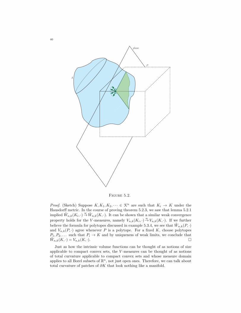
40

A

P

plane

Figure 5.2.

Proof. (Sketch) Suppose K,K1,K2, · · · ∈ Kn are such that Ki → K under theHausdorff metric. In the course of proving theorem 5.2.3, we saw that lemma 5.2.1

implied Wn,k(Ki, ·) w→ Wn,k(K, ·). It can be shown that a similar weak convergence

property holds for the V -measures, namely Vn,k(Ki, ·) w→Vn,k(K, ·). If we further

believe the formula for polytopes discussed in example 5.3.4, we see that Wn,k(P, ·)and Vn,k(P, ·) agree whenever P is a polytope. For a fixed K, choose polytopesP1, P2, . . . such that Pi → K and by uniqueness of weak limits, we conclude thatWn,k(K, ·) = Vn,k(K, ·).

Just as how the intrinsic volume functions can be thought of as notions of sizeapplicable to compact convex sets, the V -measures can be thought of as notionsof total curvature applicable to compact convex sets and whose measure domainapplies to all Borel subsets of Rn, not just open ones. Therefore, we can talk abouttotal curvature of patches of ∂K that look nothing like a manifold.

6. Recent Developments

The worst thing you can do is to completely solve a problem.– Daniel Kleitman

To conclude, we list a number of recent developments in integral geometry. Manyof these extensions have been motivated by applications in stochastic geometry[SW08]. This list is by no means exhaustive – we only cover extensions that aremore directly related to the content discussed in this thesis. A more thoroughsurvey that also covers other aspects of integral geometry can be found in [HS02].

More general sets. While convex sets (or even polyconvex sets) constitutea wide collection of objects, there have been further attempts to establish someform of Crofton’s formula or curvature measures on collections of sets with morepathological behaviors. For example, Fu [Fu94] examined “subanalytic sets” whileBrocker and Kuppe [BK00] further advanced this subject by considering “compacttame Whitney-stratified sets” (this collection includes semi-algebraic sets, suban-alytic sets, and sets belonging to an σ-minimal system). These sets show up inmodel theory and computer science.

Non-Euclidean Spaces. Starting from a given non-Euclidean space X, onecan focus on a collection of sets K ⊆ 2X and ask if we can similarly14 characterizevaluations on K in integral geometric terms. Little is known in the general contextbut Klain and Rota [KR97, chapters 3 and 11] provides some answers for the caseof X being a sphere and X being a finite set.

Crofton formula for functions. A function f : Ω→ R, where Ω ⊆ Rn is openand convex, is a convex function if and only if its epigraph is convex. This suggeststhe possibility of studying such a convex function by the techniques we explored.Indeed, for ε ≥ 0 and A is Borel set contained in Ω, one may define the ε-fatteningof A by means of f as

x+ εv | x ∈ A, v ∈ ∂f(x)where ∂f (x) denotes the “subdifferential” of f at x. It turns out that the fatteningis a Lebesgue measurable subset of Rn, and its Lebesgue measure as a function ofε is a polynomial of degree ≤ n. By considering the special case where f happensto be of class C2, these coefficients can be interpreted in terms of some expressioninvolving the eigenvalues of Hess(f) at various points (the coefficients are thuscalled Hessian measures). One can make various integral geometric definitions ofmeasures that turn out to be Hessian measures. A concrete discussion can befound in [CH05]. For comparison, a study of Hessian measures without the integralgeometric approach can be found in [TW97], [TW99] and [TW02].

Translative integral geometry. In some applications of stochastic geometry,an assumption that space is isotopic is superfluous or invalid. Thus, rather than

14We characterized all continuous invariant valuations when X = Rn and K = Kn as linearcombinations of intrinsic volume functions.

42

considering invariance under E (n), one only considers invariance under the transla-tion group T (n). The study of expectations under this setting leads to translativeintegral geometry. This subject is treated in [AF14, 1.1].

43

References

[AF14] S. Alesker and J.H.G. Fu. Integral Geometry and Valuations. Springer, 2014.[Ban67] T. Banchoff. Critical points and curvature for embedded polyhedra. J. Differential Ge-

ometry, 1:245–256, 1967.

[Ban70] T. Banchoff. Critical points and curvature for embedded polyhedral surfaces. Amer.Math. Monthly, 77:475–485, 1970.

[Bee74] G.A. Beer. The Hausdorff metric and convergence in measure. Michigan Math. J.,21(1):63–64, 1974.

[BK00] L. Brocker and M. Kuppe. Integral geometry of tame sets. Geom. Dedicata, 82:285–328,

2000.[CH05] A. Colesanti and D. Hug. Hessian measures of convex functions and area measures. J.

London Math. Soc., 71:221–235, 2005.

[DL94] R. De-Lin. Topics in Integral Geometry. World Scientific Pub Co Inc, 1994.[DO11] S.L. Devadoss and J. O’Rourke. Discrete and Computational Geometry. Princeton Uni-

versity Press, 2011.

[Fol99] G.B. Folland. Real Analysis: Modern Techniques and their Applications. John Wiley &Sons, Inc., second edition, 1999.

[Fu94] J.H.G. Fu. Curvature measures of subanalytic sets. Amer. J. Math, 116:819–880, 1994.

[HS02] D. Hug and R. Schneider. Kinematic and crofton formulae of integral geometry: recentvariants and extensions. Homenatge al professor Llus Santal i. Sors, C. Barcel i Vidal

(ed.):51–80, 2002.[Kla95] D.A. Klain. A short proof of Hadwiger’s characterization theorem. Mathematika,

42(2):329–339, 1995.

[Kni] O. Knill. Integral geometric kolmogorov quotients. In preparation.[Kni12] O. Knill. The Theorems of Green-Stokes,Gauss-Bonnet and Poincare-Hopf in Graph

Theory. http://arxiv.org/abs/1201.6049, 2012.

[Kni14] O. Knill. Curvature from graph colorings. http://arxiv.org/abs/1410.1217, 2014.[KQ03] P. Kuchment and E.T. Quinto. Some problems of integral geometry arising in tomogra-

phy. In L. Ehrenpreis, editor, The Universality of the Radon Transform. Oxford Univer-

sity Press, London, 2003.[KR97] D.A. Klain and G-C. Rota. Introduction to Geometric Probability. Lezioni Lincee. Ac-

cademia nazionale dei lincei, 1997.

[Kuh06] W. Kuhler. Differential Geometry: Curve-Surfaces-Manifolds. American MathematicalSociety, second edition, 2006.

[Lee12] J.M. Lee. Introduction to Smooth Manifolds. Graduate Texts in Mathematics. Springer,second edition, 2012.

[Lei11] T. Leinster. Hadwiger’s theorem, part 1. https://golem.ph.utexas.edu/category/2011/

06/hadwigers theorem part 1.html, 2011.[Mec98] K.R. Mecke. Integral geometry in statistical physics. International Journal of Modern

Physics B, 12(9):861–899, 1998.[Mil50] J. Milnor. On the total curvature of knots. Annals of Mathematics, 52:248–257, 1950.[Ram69] J.F. Ramaley. Buffon’s noodle problem. Amer. Math. Monthly, 76(8):916–918, 1969.

[San53] L.A. Santalo. Introduction to Integral Geometry. Hermann and Editeurs, Paris, 1953.

[San04] L.A. Santalo. Integral Geometry and Geometric Probability. Cambridge University Press,second edition, 2004.

[Sch07] R. Schneider. Integral geometric tools for stochastic geometry. Lecture Notes in Mathe-matics, 1892:119–184, 2007.

[Sch14] R. Schneider. Convex Bodies: the Brunn-Minkowski Theory. Cambridge University

Press, second expanded edition, 2014.[SW08] R. Schneider and W. Weil. Stochastic and Integral Geometry. Springer, 2008.

[Tis84] P.E. Tissier. Bertrand’s paradox. The Mathematical Gazette, 68(443):15–19, 1984.

[Tor14] S. Torniers. Haar measures. https://people.math.ethz.ch/ torniers/download/2014/haar measures.pdf, 2014.

44

[TW97] N.S. Trudinger and X.J. Wang. Hessian measures I. Topol. Methods Nonlinear Anal.,

10:225–239, 1997.

[TW99] N.S. Trudinger and X.J. Wang. Hessian measures II. Ann. of Math., 150:579–604, 1999.[TW02] N.S. Trudinger and X.J. Wang. Hessian measures III. Journal of Functional Analysis,

193(1):1–23, 2002.

[Vin08] R. Vinroot. Topological groups. http://www.math.wm.edu/∼vinroot/PadicGroups/ top-groups.pdf, 2008.

[Wey39] H. Weyl. On the volume of tubes. American Journal of MAthematics, 61(2):461–472,

1939.