Policy, Planning, and Research

WORKING PAPERS

Agriculture

Latin America and CarbbeanCountry Department II

The World BankMarch 1989WPS 163

How Infrastructureand Financial InstitutionsAffect Agricultural Output

and Investmentin India

Hans P. Binswanger,Shahidur R. Khandker,

andMark R. Rosenzweig

Prices matter - but so do banks, markets, and infrastructure.

The Policy, Planning, arid Rescsrh Cronplex distributes PPR Woriing Papers to disseminate the findings of work in progress and toencourage the exchange of ideas among Bank staff and all other intcrested in development issues Tese papers carry the names ofthe authors, reflect only their views, and should be used and cited accmdingly. lbe findings. interprctations, and conclusions are theauthors' own. hey should not be auributed to the World Bank, its Board of Directors, its management. or any of its member counries.

Pub

lic D

iscl

osur

e A

utho

rized

Pub

lic D

iscl

osur

e A

utho

rized

Pub

lic D

iscl

osur

e A

utho

rized

Pub

lic D

iscl

osur

e A

utho

rized

Pub

lic D

iscl

osur

e A

utho

rized

Pub

lic D

iscl

osur

e A

utho

rized

Pub

lic D

iscl

osur

e A

utho

rized

Pub

lic D

iscl

osur

e A

utho

rized

Plc,Planning, end Research

Agriculture

How do the decisions of farmers, financial Alfter comparing data on these factors, theinstitutions, and government agencies interact authors conclude that:and affect agricultural investment and output ina region - and to what extent are these "actors" * Agroclimatic factors continue to govern theinfluenced by a region's location and agrocli- rate at which districts can take advantage of newmatic endowments (for example, rainfall or the agricultural opportunities, and govem public,soil's moisture-holding capacity). bank, and private investment decisions.

This paper is an attempt to quantify the * The availability of banks (credit) is morerelationships of key factors, using district-level important than the real interest rate as a factor intime-series data from India. aggregate crop output and farmers' demand for

fertilizer. Rapid bank expansion in an areaAgricultural opportunities in a district are increased fertilizer demand by about 23 percent,

seen as the joint outcome of the agroclimatic en- rates of investment in pumps 41 percent, in milkdowments of the district and new technology animals 46 percent, and in draft animals aboutthat becomes available to it. Better agroclimatic 38 percent. Despite their impact on investmentopportunities improve output (relation 1), but and fertilizer use, the impact of banks on outputalso increase the economic return for a private appears to be fairly small (nearly 3 percent).farm investment - say, in a tractor (relation 2).Greater private profit in a well-endowed region * Unsurprisingly, commercial banks prefer toinduces farmers to press for more investment in locate in well-watered areas where the risk ofinfrastructure (relation 3). Financial institutions drought or flood is relatively low. Bank expani-find it more profitable to locate where there is sion is facilitated by government investments inmore demand for capital and more repayment roads and regulated markets, which improvecapacity (relation 4) and where good infrastruc- farmers' liquidity and reduce banks' and farm-ture reduces their costs (relation 5). Private ers' transaction costs.agricultural investment and use of input is moreprofitable the better the agricultural opportuni- * In the 1970s, expansion of regulatedties (relation 2), the better the infrastructure markets contributed 4 percent to growth of(relation 6), the cheaper the cost of financial agricultural output and 17 percent to demand forservices (relation 7), and the more favorable fertilizers. Expansion of electrification in-government's price and interest policies (relation creased output 2 percent in a decade by increas-8). Exactly the same factors affect the output ing investment levels for pumps and fertilizer.supply (relations 9, 10, 11). Traditional ap- A primary education added a large 8 percent toproaches to production function estimate the crop output over the decade, primarily bydirect impact of capital stocks (investment) and increasing fertilizer demand nearly 30 percent.input use on output (relation 12), ignoring manyof the factors discussed here.

This paper is a product of the Agriculture Operations Division, Latin America andCaribbean Country Department IT. Copies are available free from the World Bank,1818 H Street NW, Washington DC 20433. Please contact Josefina Arevalo, room17-100, extension 30745

The PPR Working Paper Series disseminates the findings of work under way in the Bank's Policy, Planning, and ResearchComplex. An objective of the serics is to get these findings out quickly, even if presentations are less than fully polished.The findings, interpretations, and conclusions in these papers do not necessarily represent official policy of the Bank.

Produced at the PPR Dissemination Center

THE IMPACT OF INFRASTRUCTURE AND FINANCIAL INSTITUTIONSON AGRICULTURAL OUTPUT AND INVESTMENT IN INDIA

byHans P. Binswanger, Shahidur R. Khandker,

and Mark R. Rosenzweig

Table of Contents

I. Introduction ....................................... 1

It. Analytical Framework. 3

III. Data and Variables ................................. 11

IV. Agroclimatic Endowments, Infrastructure,Population and Crop Output ......................... 17

V. Development of Commercial Banks .................... 22

VI. Determinants of Private Investment ................. 24

VII. Determinants of Fertilizer Demand and AggregateCrop Output ........................................ 31

VIII. Discussion ......................................... 35

References ............................................... 42

I. Introduction

Government expenditure on physical infrastructure and human

resource development influence the private production and investment

decisions in agriculture and thus are essential ingredients of increased

agricultural productivity. Government investments (both physical and

human) can directly increase agricultural output by shifting the production

frontier as in the case of irrigation. This is what might be called the

direct effect of government infrastructure. Government investment also

increases the rate of return to private agricultural investment and thereby

leads to greater investient and output. Moreover, by increasing the

viability and profitability of financial intermediaries,.infrastructure can

facilitate the emergence and growth of financial institutions that increase

access to working and investment capital or reduce the costs of borrowing

for long-term investment. Better credit facilities, by enab}ing the

smoothing of consumption, may also increase the willingness of farmers to

take risk.

11 This paper would not have been feasible without the patient andpersistent efforts of a large number of people who assembled, checkedand processed the enormous data base required. The ICRISAT economicsstaff graciously provided their district data base for the semiaridtropics. Robert Evenson and Ann Judd in turn contributed their NorthIndia district data base. James Barbieri assembled the data requiredto update these data bases to 1982, added additional states, andcollected the data on banking, on private capital stocks andinvestment. He was advised in this endeavor by Devendra B. Gupta whoprovided the liaison with the respective Indian authorities who weregracious to release data which were still in manuscript form. Dr. D.R.Gadgil opened the data base of NABARD and personally organized the

Continued on next page

-2-

Thus agricultural output and investment respond to the separate

actions undertaken by three economic actors-- faxsers, government agencies

and banks. All three actors respond positively to agricultural

opportunities implied in the agroclimatic endowments of a region and in new

technologies when it becomes available. The magnitude of the effects

depends on how each of the actors responds to agricultuzal opportunities

and how farmers and banks respond to the government investment decisions.

This paper seeks to quantify the inter-relationships among the investment

decisions of governmeat, financiaI institutions and farmers and their

effects on agricultural investment and output.

The central problem of estimating these relationships is that,

once government agencies and banks are admitted as actors who respond to

agricultural opportunities,. one can no longer take the distribution of

government infrastructure and banking iastitutions as exogenously given or

randomly distributed. The impact of government infrastructure on

investment and output is likely to be more pronounced in a better endowed

region than in a poor endowed region and governments will therefore invest

more where opportunities are greater. The resulting unobserved variable

problem may be circumvented by either a precise quantitative

characterisation of the agroclimatic potential or by using the fixed

effects technique of estimation. For analyzing growth in aggregate output

Continued from previous pageassembly of the banking data. Apparao Katikineni organized thescreening, and further computer processing of the many different anddisparate data bases which had to be merged into a single data base.Kathy Graham did all of the cartographic measurements. We were alsoassisted by Sneylata Gupta and Dan Ghura.

-3-

both Binswanger, Yang, Bowers and Mundlak (BYBM, 1986) and Lau and

Yotopoulos (1988) have implemented the appropriate fixed effects technique

using time-series x cross section data of countries.2

The paper is structured in the following order. Section II

outlines an analytical framework. Section III describes the data and

discusses the variables. Section IV shows how various agroclimate

variables affect government decision on where to build roads, markets and

schools and where to provide electricity and canal irrigation. Section V

looks at the joint impact of agroclimatic endowments and infrastructure on

the growth of financial intermediaries. We do this in a cross-section and.

time series framework using district level data from India. Section VI

then considers the joint determination of private agricultural investment

as functions of agroclimatic endowments, technology change, infrastructure,

financial intermediaries and of price and interest policy. In Section VII

we estimate the impact of the same variables on fertilizer demand and

aggregate crop output. The results' are summarized in the concluding part

of the paper.

II. Analytical Framework

In our framework (see Figure 1), agricultural opportunities in a

district are the joint outcome of the agroclimatic endowments of the

district and the new technology which becomes available to the district

2/ Bapna, Binswanger and Quizon (BBQ, 1984) used random effects techniquesto analyze output supply in time-series x cross section data ofdistricts in India.

AGRICULTURALOPPORTUNITIES 0 PRIVATE

- AGROCLIMATIC agroclimate effects () INVESTMENTSENDOWMENTS AND INPUT USE

- NEW TECHNOLOGY financial\ ~~~~~~~syste ;f f t /-

prod. policy effectsgrntr) function

pressuregroups ~~~~~~~~~~~~~~~~~~PRICE AND

| ~~~~~~~~~FINANCIAL direct effects /INTEREST< t>~ ~ ~~) INSTITUTIONS /.POLICY

effeo lcts effects

infrastructure effects (IQ|

Figure 1: Major Relationships among Agroclimte Radowents,?1nanclal Institutions, Government Infrastructure andAgrliltural Investment and Output

-5-

from industry and from foreign, national and state research systems.3 T:^e

same technology is potentially available to all districts., but the exten:

to which it is actually applicable to a given district depends on its

agroclimatic endowments. For exampli high yielding varieties of wheat are

not relevant for districts with high wdnter temperatures or districts with

excessive amounts of rainfall and flooding problems. Thus the size and the

growth of the set of agricultural opportunities varies across a district

according tu their agroclimatic characteristics.

Better agroclimatic opportunities such as better rainfall, a

higher moisture holding capacity of the soil and a better irrigation

potential directly affect agricultural output (relation 1). But better

opportunities also increase the economic return to private farm investments

such as tractors; draft animals or pumpsets (relation 2). The greater

private profitability of agriculture in well endowed regions induces

farmers to press government for increased investment in the supportive

infrastructure (relation 3). Financial institutions find it more

profitable to locate in environments where a good agroclimate and rapid

technical change leads to a substantial demand for agricultural investment

and-working capital and a high repayment capacity (relation 4) and where

good infrastructure reduces their cost of intermediation (relation 5).

Private agricultural investment and input use is more profitable the better

the agricultural opportunities (relation 2), the better the government

3/ Although technology investments are Lhemselves government decisionvariables, for the purpose of this paper technology is treated asexogenous to the decisionmaking of specific-government agencies, banksand farmers when they make investment, location and input decisions.

-6-

infrastructure (relation 6), the cheaper the cost of financial services

(rel&tion 7) and the more favorable price and interest policies are which

are pursued by the government (relation 8). Exactly the same factors

affect the output supply. (relation 9, 10, 11). This means that

agricultural opportunities must be translated into public and private

investment 'fforts in order to affect agricultural output (For a discussion

see BYBM, 1986 and Mundlak, 1985).

The traditional production function approach has attempted to

estimate the direct impact of capital stocks (investment) and input use on

output, (relation 12), ignoring much of the factors discussed here and all

the simultaneity problems (see for example Hayami and Ruttan, 1986).4

Estimation Equations and Econometric Specifications

Let Rrjt be the level of the r-th infrastructure variable (say.

roads) in district j at time t. As agroclimate variables ar-e strictly

exogenous, the dependence of the infrastructure variables on a set of

measured agroclimate variables and location factors ai can be estimated

simply in a cross section regression -

(1) Rrjt Rrjt (0j, Ppj ejt)

4/ A profit-oriented producer will take input and output decisionsjointly. In order to deal with this simultaneity, the correct way toestimate the production function (12) is to use the predicted insteadof actual levels of capital stocks and other inputs. However, asclearly apparent from figure 1, we do not have any instruments whichaffect only the inputs but not the output. -Therefore the productionfunction cannot be estimated econometrically.

-7-

where p3 is the effect of unmeasured agroclimatic and location factors, and

ejt is a time-specific error term. 5

Financial institutions in turn are assumed to locate in districts

with good agroclimate and infrastructure, i.e.

(2) Bjt - Bjt (Rjt, aj, jj, Tjt, ejt)

where Bjt stands for the number of banks operating in the district at time

t, Tjt is a region-and time-specific technology index, and ejt is an error

term specific to the banking equation.

The simultaneity between banks, Bjt, and infrastructure, Rjt,

arising from their joint dependence on unobserved agroclimatic variables,

, can be overcome if an additive model is chosen such as

(3) Bjt aO +aj Rjt + a2 Uj +a3 IJ + Tjt + ejt

For the mean overtime in district j this relationship reads

(4) Bj. 3 ao + al Rj. + a2aj +a3 /pj + Tj. + ej.

Taking the difference of these equations, i.e. by transforming the

variables to differences from their means, leads to the following

estimation equation in terms of difference from the means

(5) (Bjt - Bj.) - al (Rjt - Rj.) + (Tjt - Tj.) + (Ejt - ej.)

5/ Similar ultimate reduced forms can be established for all otherendogenous variables in the system, the banks, private investment andoutput. However, the reduced forms for output, for example, is notvery informative as it includes both the direct or technical impact ofthe agroclimate on output (relation (1)) as well as all the indirecteffects via its impact on infrastructure, banks and private investment.

As et is a randomly distributed error torm which is uncorrelated

with oj and Rjt, relationship (5) can be estimated by the Ordinary Least

Squares technique.

The disadvantages of using this fixed effects model is that the

direct impact of the agroclimate (i.e. relation (4)) cannot be estimated. 6

These direct effects could only be estimated (in this and all subsequent

equations) if the infrastructure variables were randomly distributed acrc-s

the districts, i.e. were not dependent on the unobserved agroclimatic

variables pi. This could happen if the measurement of the observed

agroclimatic variables oj were so good that no unobserved effects were left

over to significantly affect the infrastructure investments. In that case

a random effects model would be appropriate. We will use Hausman-Wu

specification tests to determine whether to use the fixed effects or random

effects model and present results accordingly.

Private agricultural investment in capital item k (say draft

animals or tractors), depends on the agroclimate, the infrastructure and

the banks. In addition it depends on policy variables such as the output

price P, the fertilizer price Pf, and the real interest rate r, i.e.

(6) lkjt - Ikjt (Kjt-I, Pf3jt' jt' B3jt Rjt, Tjt, 'jp Pjt ejt)

where Kjt-l is the capital stock of year (t-1). In these equations the

6/ As discussed in footnote 1, it cannot be estimated either in a reducedform equation of the form of equation (1).

-9-

simultaneity problem between Bjt, Rjt, and p can be overcome just as for

equation (3) by using the fixed effects technique. For the interest rate,

however, a simultaneous equation problem may arise if higher investments

demand leads credit s npliers to raise the interest rate. In the

application .below this problem is minimized by the fact that the interest

rate used is fixed by the government of India. Only if the government

specifically takes agricultural investment demand (rather than more

aggregate credit conditions) into account in fixing the interest rate will

the simultaneity problem persist. For the other prices a simultaneity can

also arise if increased investment leads to higher output supply (and

fertilizer demand) and therefore lower output prices (higher fertilizer

prices). The fertilizer price used below As the railhead price set by the

government and the endogeneity problem is likely to be minimal. However,

in order to overcome the simultaneity problem associated with output prices

we use an index of international commodity prices as an instrumental

variable for the domestic price index. *As India is a small country in

virtually all international agricultural commodity markets, this completely

eliminates the simultaneity bias.7 The index of international commodity

prices is computed separately for each district using district-specific

production weights for the year 1975. Since agricultural wages are clearly

endogenously determined with agricultural output and investment we replace

this variable with state-specific urban wages as an instrument.

7! India has state trade in agriculture. So the domestic prices do notcorrespond in any simple way to international prices. Nevertheless,estimates show that domestic prices respond positively to internationalprices, with a lag of 3 to 4 years.

- 10 -

As can be seen from figure 1, the variables entering the aggregate

crop supply equations are exactly the same as those entering the investmen:

equation and all estimation problems are the same.

Obviously no data exist on the district-specific index of

available (but not necessarily implemented) technology Tjt. Evenson and

Kislev (1975), BYBM (1986) and others used expenditure data, or manpower

data for public research and for extension. (Alternatively Boyce and

Evenson (1975) has used research publications). However, data for these

variables do not Wxist at the district level. Moreover they do not include

technology opportunities arising from private industry and seed

corporations. Other researchers have used simple time trends to proxy

technology opportunities (e.g. Binswanger, 1974). However, simple time

trends assume technology opportunities grow at constant and identical rates

in each district. But the point is that agroclimatic endowments affect the

extent to which new technology option; are applicable to a district. Hence

technology trends must differ across districts. If, for example, banks

systematically located in districts where the green revolution had raised

the input and borrowing requirements of farmers, an output supply function

including common time trends and banks would erroneously allocate to banks

a part of the output contribution of technology, i.e. the coefficient of

banks would be upwards biased. In order to circumvent this problem the

district specific technology trend is entered into the models as follows:

(7) Tjt - Ebm amj t + bttm

The regression include a common time trend and interaction terms

of all the agroclimatic variables with the time trend, and the district

- .11 -

specific time trend is an estimated function of time and time x climate

interactions. 8 For example in the output supply equation one would

expect the interaction between time and irrigation potential to be

positive, consistent because high yielding varieties of rice and wheat

require good control over water and soil moisture.

III. Data and Variables

The data we have used here are drawn from India. The cross-

section units are 85 randomly drawn districts of India. These 85 districts

belong to 13 states of India--Andhra Pradesh, Bihar, Gujarat, Haryana,

Jammu and Kashmir, Karnataka, Kerala, Madhya Pradesh, Maharashtra, Punjab,

Rajasthan, Tamil Nadu and Uttar Pradesh. The 85 districts are part of the

99 districts from 17 states randomly drawn by the India's National Council

for Applied Economics for its well known Additional Rural Income Survey.9

The period covered in this paper is the agricultural years 1960/61 to

1981/82. The study period covers the agricultural years 1960/61 to

1981/82, but for some dependent variables with more limited data

availability shorter periods are used.

8/ Alternatively one could introduce a trend for each district separatelyas in Lau and Yotopoulos.

9/ In fact, 80 districts are drawn from NCAER sample, while the remaining5 districts are the ICRISAT districts. All NCAER districts could notbe included because of deficiencies in the data for both primary andsecondary districts.

- 12 -

TABLE 1: Descriptive Statistics of Variables

Variable Number of Mean StandardObservations Deviation

Dependent variablesAggregate crop output index 1785 1.192 1.045Fertilizer consumption,nutrient tons/10 sq. km 1148 22.054 924.045

Net investment in draft animals;numbers per year/10 Sq.Km 304 4.962 15.504

Net investment in tractors;numbers per yearllO Sq.Km 304 0.119 0.260

Net investment in pumps; numbersper yearilO Sq.Km 304 1.343 1.864

Net investment in milk animals;numbers per year/10 Sq.Km 304 13.555 25.489

Net investment in small stocks;numbers per year/10 Sq.Km .304 5.308 15.291

Rural population, numbers/10 Sq.Km 1785 2070.304 1547.327

Time-varyina independent variablesCanal irrigation, '000 ha/10 Sq.Km 1785 0.064 0.099Number of villages with primaryschools/10 sq. km 1785 1.139 0.605Electrified villages, numbers/10 Sq.Km 1785 0.688 0.764Commercial banks, numbers/10 Sq. Km 1785 0.069 0.108Regulated niarkets, numbers/10 Sq.Km 1785 0.014 0.022Road length, '000 km/10 Sq.Km 1785 4.389 4.277Real interest rate of cooperativesocieties 1785 4.010 4.485

Aggregate real domestic crop- price index 1785 0.968 0.295Aggregate Real InternationalPrice index 1785 0.687 0.355

Real urban wage (annual earnings) 1785 A186.336 1195.586Real fertilizer price index 1785 3.413 0.505Annual rainfall (in mm) 1785 1138.573 986.503

Time-invariant independent variablesLength of rainy seasonin months 85 3.653 1.368

Number of excess rainy months 85 1.236 1.393Number of cool months(Temp < 180) 85 0.935 1.313

Percentage of district arealiable to flooding 85 1.389 3.531Irrigation potential, percentage 85 30.001 31.897Urban distance (km) 85 298.441 152.029Soil moisture capacity index 85 2.350 1.009

- 13 -

For each district the aggregate crop output is the index of 20

major crops with district-specific prices of 1975/76 as the base. -

Agricultural investment is represented by private investment in draft

animals, milk animals, small stock (i.e. sheep and goats), tractor, and

irrigation pump. Investment for each period is the difference in the

stocks meaiured for each of the agricultural censuses which occurred at

five year or six year intervals. It is therefore net investment per year

during each of four intercensal intervals. Government infrastructure

consists of primary schools, canal irrigation, rural electrification,

regulated rural markets, and total road le.ngth. The only rural financ.al

intermediary is the number of rural branches of Commercial Banks--the only

-comparable data available for the study period 1960-81. The variables that

characterize the district's agroclimate environment are the irrigation

potential, the length of the rainy season in months, the number of months

in a year with excessive rain (where rainfail exceeds potential

evapotranspiration),l0 the number of cool months in a year when mean

temperature is less than 18 degree Farenheit (this is related to the

ability to grow wheat), the proportion of a district liable to flooding, an

index of the moisture capacity of the soils in the district, and the

district's distance to the nearest major urban center (out of eight centers

i.e., Delhi, Bombey, Madras, Banglore, Kanpur, Ahmedabad, Hyderabad and

Calcutta). The price variables consist of the annual per capita earnings

of industrial workers as a proxy for urban wages, a price index of

fertilizers at railheads, the rate of interest charged by the Primary

Agricultural Cooperative Societies, and the district specific real

10/ Evapotranspiration is a sum of transpiration via plants and evaporationfrom soil.

- 14 _

international price index for the aggregate output. The international

prices of 17 crops have been converted to Rupees at the official exchange

rate and aggregated using district-specific production weights for the

agricultural year 1975/76. Domestic price indices using district level

farm harvest prices have also been computed for comparison. All the prices

or price indices are deflated by the consuner price index for rural workers

using 1975/76 as the base year. The interest rate charged by cooperative

credit, societies is the expected real rate i.e., the nominal rate for the

current year less the average percentage increase in the consumer price

index for the previous five year, i.e. inflationary expectations are

assumed to form over a five-year period.11 The means and standard

deviations of these variables are listed in table 1.

The data relating to the agroclimate and the urban distance are

single data points for each of the 85 district, because they are the

permanent characteristics of each district. The data relating to

agricultural output, government investment, prices and Commercial Banks are

time-series data covering the period, 1960/61-1981/82. In contrast, the

investment data refer to the four intercensal periods 1961-66, 1966-72,

1972-77, 1977-82. When investment equations are estimated the independent

variables are their respective means over the corresponding census

intervals.

11/ In both the output supply and investment equations, the inflation ratesare averaged over five years, except for the years prior to 1965 wheredata limitation led us to use averages for 2, 3 and 4 yearsrespectively. The rate of inflation did not fluctuate sharply in thelate fifties, or early sixties.

- 15 -

The following variables require additional explanation: The

azzregate output index reflect both variation over time in each district

relative to its base year 1975 as well as variations in output across

districts relative to a hypothetical average district formed by computing

the averages of all variables across districts in 1975. The agregate

output is normalized for district size, i.e. it c-mpares aggregate "yields"

per unit of geographic area. When fixed effect techniques are used the

across- di-trict variability is of course lost.

'Rezulated markets do not include all rural markets but only those

where government provides market infrastructure and regulates all trades

via a supervised auction system. The government does not regulate the

market price but may enter as a purchaser in order to prevent market prices

from falling below its guaranteed level.

The rural banking system is complex. It consist of traditional

moneylenders and traders for whom no data exist. Cooperative credit

societies were the first formal institutions to achieve wide rural

coverage. They lend largely for short-term production purposes such as

fertilizers. By 1969 such societies existed in virtually all districts of

India covering 94 percent of the villages in the country and they were

providing 5i percent of total formal credit extended to famers. Their

number has been declining as smaller societies have been merged in recent

years. Yet by 1979 they were providing 49 percent of all formal credit.

We include the regulated government lending rate of these societies among

the explanatory variables. At this regulated interest rate credit

rationing is pervasive and we test whether the rate has an influence on

- 16 -

output and investment despite the rationing. Land Development Banks are

also cooperative institutions which lend primarily for investment purposes.

Between 1969 and 1979 their share of lending in formal credit increased

from 15 percent to 19 percent. Their lending rates are closely tied to the

official rates of the Cooperative Credic Societies, i.e. the interest

variable will capture the effect of interest rate changes of both the

cooperative credit societies and the Land Development Banks.

The Commercial Banks, in 1960, were not involved in lending to

farmers except perhaps to plantations and very wealthy farmers. However,

they did considerable lending to agroindustrial enterprises. After their

nate 'alization in 1969 they were compelled by the government to expand

their lending to farmers and agroindustry with targets set both for number

of rural branches as well as the proportion of lending to the agricultural

sector. Between 1969 and 1979 the share of commercial banks in formal

credit provided to farmers rose from 34 percent to 49 percent at the all

India level. In the 85 districts considered here the role of commercial

banks rose even farther. Their share in formal credit rose from 52 percent

in 1972 to 72 percent in 1.979. At the same time the number of rural and

semi-urban commercial bank branches rose from 3,625 to 7,690. Unlike the

volume of lending and outstanding loans in any period, which is influenced

by farmer demand, the number of branches is strictly controlled by the

Banks and'therefore strictly exogenous to farmer decision making. Other

than for the joint dependence of farmer and bank decision making on

agroclimatic and infrastructure variables, no endogeneity problem therefore

arises. Unfortunately the number of Cooperative Societies and Land

Development Banks cannot be used in these equations as exogenous measure of

the growth of these systems because the process of consolidation has

- 17 -

reduced their numbers but not necessarily the availability of their

services in the affected villages.

Soil moisture capacity is a variable which can be viewed as a

substitute for either rainfall or irrigation. For a given rainfall a

higher soil moisture capacity means that a crop can withstand more days

without additional rainfall. In addition where soil moisture capacity is

yery high, a full moisture reservoir in the soil may be able to support

several months of a crop cycle without the addition of rainfall or

.irrigation. FQr given annual rainfall, payoffs to irrigation investments

ara therefore more limited where soil moisture capacity is higher.

Irritation potential is defined as the percentage of a district's

area inside any type of irrigation command area, i.e.. sum of proposed.

command area, command area under construction and already existing command

area.12 This-variable has been measured using the Irrigation Atlas of

India. Planned command areas are a good indicator o. the remaining

potential for canal irrigation in India as they reflect long range plans

and any area not yet included in these plans has virtually no potential.

IV. Azroclimatic Endowments. Infrastructure. Population and Crop Output

In Table 2 we see that the seven measured agroclimatic and

location factors explain between 24 percent of the variation in the density

of primary schools to 41 percent of the variation in government provided

12/ An irrigation command area is an area whilc receives or is expected toreceive water from an irrigation system.

- 18 -

Table 2: Effects of Aprocilmat. Endowment. on Infrastructure. Population

and Asaresate Crop Output

(Observation a 56)

Explanatory Rural Regulated Canal Primary Rural AggregateVariables Road Morket Irrication School Electricity Population Crop Output

Cool months -0.222 0.004 0.912 0.303 0.389 285.725 6.229(-0.587) (1.647)e (1.559) (4.770). (4.293)o (2.261)o (2.417)*

Excoss rain 0.229 -4.O02 -0.M1 -0.041 0.009 42S.138 0.019(0.477) (-0.761) (-4.667) (0.077) (2.679)* (2.679). (O.168)

Rainy seson 2.442 -4.064 9.oo7 0.079 0.089 S41.898 0.264(4.901)e.(-0.140) (0.708) (0.988) (6.775) . (3.86). (2.261)*

Flood potential -0.077 -O.01 -O .W14 0.021 -0.064 -10.649 -0.694(-4.S09) (-1.622). (-1.234) (9.862)- (-1.826)o (-0.226) (-2.574).

Irrigation 0.033 0.001 0.002 0.003 6.W69 20.589 0.034potential (1.93S). (5.872)o (6.706)o (1.127) (2.332). (3.712). (8.262).

Soil moisture 0.422 0.004 -0.619 0.116 0.231 -14e.635 0.102capacity (1.676). (2.827). (-2.187). (2.159)* (-0.982) (-8.034) (0.914)

Urban distance -4.003 0.0W04 0.6001 4.0002 -0.001 -0.671 0.034(-9.118) (2.881)- (2.266). (-0.320) (-1.419) (-0.825) (0.026)

Constant -4.218 -.. 014 -0.018 0.586 0.186 -416.025 -0.804(-1.692). (-9.97) (-9.384) (1.474) (0;826) (-4.524) (-1.852)

Adjusted R-cquarr 0.87 6.8 0.48 0.24 9.28 0.41 0.53

Not.s: t-Statisticu are in parentheses. Asterisk refers to significance level ot 10 percent orbetter. Rural road corrosponds to the agricultural year 1974, while the remainingvariables relate to agricultural year 1981.

- 19 -

irrigation and the population density of the region. The explanatory

power is thus very substantial, not much smaller than that for output

itself (53 percent). The traditional treatment of agricultural

infrastructure as exogenous variables in output supply analysis is

unwarranted.

The variable with the most powerful effect across the equations is

irrigatiorn potential, i.e. the proportion of the area which is included in

an existing or planned irrigation command area. It significantly increases

the density of all infrastructure variables, except schools. It is also

clear that population has migrated to, or grown more rapidly in regions

with a high irrigation potential, i.e. private and public decisions are

influenced by the same factors.

For the other variables the impact varies substantially across the

government investments. Regions with a fairly cool winter, which are able

tRo grow wheat, have higher density of regulated markets, more primary

schools, more electrification and higher population density. Population

density is also very high in regions with many monthn with excess rain,

i.e. the humid tropical zones such as Kerala. Population and roads are

higher the longer the rainy season, or said otherwise, government has found

it less worthwhile .to build roads in semiarid and arid regions. Areas

which are liable to flooding are not well served by regulated markets,

roads, and electrification. As discussed in the data section, the results

show that high soil moisture capacity acts as a substitute for canal

irrigation. But high soil moisture capacity is a positive agroclimatic

attribute and thus attracts investment in regulated markets, roads and in

electrification. Distance to major urban centers tends to increase the

- 20 -

Distance to major urban centers sends to increase the density of regulated

rural markets, and also the level of government provided irrigation.

One point which stands out from the regressions is that for the

purpose of government infrastructure investments, agroclimatic potential

cannot be measured by a single variable or an agroclimatic index.

Different aspects of the endowment affect the govrernment investments

differentially.

The total effects--both direct and indirect effects via government

infrastructure and banks--of agroclimate and location factors on output

supply are also shown in table 2. They suggest that agroclimatic

endowments explain 53 percent of the variation in agricultural production

of 85 districts in the agricultural year, 1981. Agricultural output supply

is high in regions well endowed with water from either irrigation or

rainfall. Regions with a relatively cool winter have high agricuitural

output while agricultural output is low in regions with a high flood

potential. All the effects are as-expected.

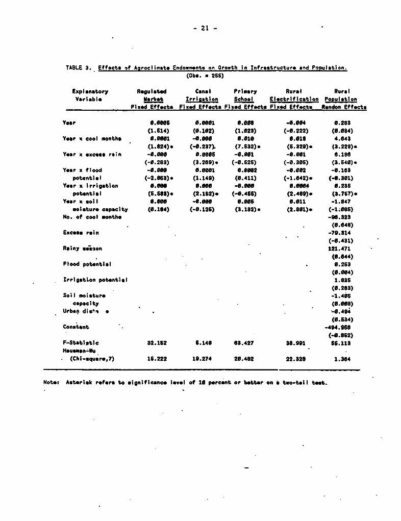
Using data for the three-census years (1961, 1910, 1981) we

investigate in table 3 whether the investment trends over the past two

decades were similiarly influenced by the agroclimatic characteristics.

This is done in regressions which include time trends according to equation-

7, i.e. interactions between time and the agroclimatic characteristics.

The Hausman-Wu test suggests that a fixed effects model is appropriate for

explaining variation in public infrastructure ovdr time, while a random

effects model can be used for rural population growth.

- 21 -

TABLE 3. Effects if Agroclimate Endowments on Growth in Infrastructure and Population.(Obe. a 265)

Explanatory Regulated Canal Primary Rural RuralVariable Market Irrication School Electrification Population

Fixod Effeets Fixed Effects Fixed Effects Fixed Effeets Random Effects

Yoor 0.0006 0.0001 0.008 -0.004 0.283(1.614) (0.162) (1.623) (-0.222) (t.034)

Yoor A cool months 0.0001 -0.000 6.010 0.018 4.643(1.624). (-0.237). (7.632)* (5.329). (3.229).

Year x excess rain -0.000 0.0005 -0.001 -0.001 6.186(-0.283) (3.269)* (-0.526) (-0.305) (3.640)*

Yoar x flood -0.000 0.0001 0.0002 -0.002 -0.163potential (-2.063)o (1.149) (0.411) (-1.042). (-4.361)

Year a lrrigation O.WO 0.60 00 0.66 6.0104 0.235potential (5.683)0 (2.152)* (-0.456) (2.489). (3.757).

Year x soil 0.6of -e.00o 0.005 0.011 -1.847moisture capacity (0.184) (-0.126) (3.132)o (2.801). (-1.0S5)

No. of cool months -96.S23(0.648)

Excess rain -79.314

(40.431)Rainy season 121.471

(6.644)Flood potential 0.2S3

(0.004)Irrigatton potential 1.835

(0.283)Soil moisture -1.406

capacity (0.008)Urban dish, g --S.494

(0.534)Constant -494.96C

(-0.852)F-Statiptic 32.152 C.148 63.427 38.991 56.113Hausen-Wu

(Chi-square,7) 16.222 19.274 20.482 22.326 1.364

Note: Asterisk refers to sIgnifIcance level of 10 percent or better on * two-tall teat.

- 22 -

The results are consistent with the simple cross section results.

They suggest that better agroclimatic attributes such as irrigation

potent!al contribute to the growth in public infrastructure as well as

population, while unfavorable attributes such as flood potential reduces

their growth over time. This clearly indicates that agroclimatic

endowments did not only affect the placement of public programs and

institutions in the distant past, but also their growth over the study

period.

V. Development of Commercial Banks

In Table 4 the cross-section results indicate that Commercial

Banks have tended to locate in areas which are well endowed with water,

either from irrigation or from a long and over-abundant rainy season. Such

areas are characterized by relatively low risk of agriculture and therefore

less repayment'problems for the banks (Binswanger and Rosenzweig, 1986).

Th. implies that the banks have avoided areas where drought risk is high.

That banks try to avoid'high-risk areas, is also apparent in the negative

coefficient of flooding potential.

The simple cross section relation for the year 1980 included the

indirect effects of the agroclimate on Bank, via the improved

infrastructure. The pure infrastructure effects, on the other hand, are

estimated and peesented in Table 4 using the cross-section time-series data

of 85 districts for the years 1972-80. As the results of the Hausman-Wu

test suggest, the fixed effects model appears more appropriate than the

random effects model in explaining the variation in the bank growth over

time and only the fixed effects results are therefore shown. The

-23 -

TABLE 4: Effects of Azcoclimatic Endowments andGovernment Infrastructure on Commercial Bank

Cross-section effects Fixed effectsExplanatory Variable (observations * 85) (observations - 765)

Year 1980

Canal irrigationa -0.193(-2.190)*

Regulated Marketa 0.196(3.227)*

Primary Schoola 0.026(0.077)

Rural Electrificationa -0.115(-1.457)

Roada 0.821(4.584)*

Year -0.011(-4.873)*

Year x Cool Months 0.002(3. 835)*

Year x Length of 0.002Rainy season (4.514)*

Year x Flood Potential -0.001(-3.983)*

Year x Irrigation 0.0001Potential (6.639)*Year x Soil Moisture -0.0001Capacity (-0.093)

Year x Excess Rain Months 0.005(11.372)*.

No. of Cool Months 0.016(1.156)

Length of Rainy Season 0.046(2.735)*

Flood Potential -0.010(-1;992)*

Irrigation Potential 0.002(3.848)*

Soil Moisture Capacity 0.0002(0.068)

Excess Rain Months 0.050(2.985)*

Urban Distancea -0.205(-0.089)

Constant -0.132(-1.570)

F-Statistic 6.90 94.792Hausman-Wu (Chi-square, 12) 51.631

NOTE: t-Statistics are in parenthesis. Asterisk refers to significancelevel of 10 percent or better.a Coefficients of these variables are in elasticity form.

- 24 -

regression clearly shows that Banks are more likely to locate in areas

where the road infrastructure and the marketing system are improving.

Markets provide both higher incomes to producers and reduce the price risk

they face, i.e. they improve their repayment capacity. And roads have an

eifect on farmer income, demand for inputs and hence credit and they reduce

the credit transactions costs of both the customers and the banks. Of the

two variables, roads have the most powerful effect with an elasticity of

about 0.83, followed by regulated markets with an elasticity of 0.20.

Markets, of course, are a relatively cheap investment which can be

increased much more rapidly than roads. Rural electrification does not

contribute to Bank gro-th. Indeed it has a negative effect which is

statistically significant at the 10 percent level.

The time trend and the interaction effects with time confirm that

Bank growth has been more rapid in districts with a high irrigation

potential, where the rainy season is longer, and where cool months allow

for the growth of wheat. This is fully consistent with the hypothesis that

banks have systematically located in environments which were favorable to

the green revolution technologies; i.e. that banks responded to

opportunities.-created by technical change. In addition bank growth was

lower where the flood potentially high, i.e. where they face higher risk

and where green revolution technology is less applicable because of lack of

water control.

VI. Determinants of Private Investment

The investment data in table 5 relate to average annual levels of

investment for each of the intercensus intervals for which we have data.

- 25 -

Table S. Effects of Aaroclimatic Endowments. Government Infrastructuro.Commercial Bank *nd Prices on Agricultural Investment

(No. of Observations u 304)

Investment InExplanatory Draft Milkvariable animals animals Small stocks Pumos Tractors

Aggregote real interno- 2.098 1.007 1.697 -0.497 -0.076tional price, logged a (3.709)* (2.368)* (2.163)* (-1.327) (-0.197)

Real fertilizer price5 -12.262 -8.396 -7.836 -1.140 -1.127(-4.292)* (-4.139)* (-2.662)* (-0.834) (-0.799)

Real urban wag, a 6.866 3.406 2.106 -0.470 1.127(6.306). (5.684S) (1.977). (-0.922) (2.284).

Real interost rate -0.686 -6.115 -0.302 -0.109 0.092(.3.688). (-1.163) (-1.691)§ (-1.162) (6.962)

Roads a -2.128 -1.443 1.186 0.107 -0.319(-3.228). (-4.002)* (1.808)- (0.362) (0.983)

Canal irrigation a -0.198 -0.074 0.756 -0.067 0.481(-0.327) (-0.220) (1.238) (-0.260) (1.616)§

Primary schools * .3.815 0.686 -0.949 -0.782 0.037(2.341). (6."65) (-0.696) (-1.233) (0.047)

Electrification a 9.713 0.526 -0.157 6.56S -0.031(1.967). (2.634)* (40.428) (2.072). (-0.173)

Commercial banks a 0.636 0.849 0.657 0.375 0.143(2.492). (7.146)* (3;046)* (3.6806) (1.310)§

Regulated-markets a -0.066 0.212 0.225 -0.041 D .16V.(-6.184) (1.119) (0.649) (-0.246) (0.910)

Rainfall x 1O3 1.506 11.309 -8.241 0.287 0.042(0.362) 'i-801)* (-1.871). (6.711) (0.867)

Past stock -0.183 -0.688 -0.139 -0.047 0.134(-12.62S). (-2:099). (-12.656). (-4.983)* (10.704).

Year -1.740 -1.160 -0.773 0.104 0.002(-3.199)* (-1.438) (-1.340) (1.412) (0.259)

Year x cool month* 0 083 -0.289 0.408 0.028 0.002(0-.813) (-1.912)* (3.748)* (2.119). (1.486)

Year x rainy season 0.136 0.693 0.127 -0.001 -6.661(1.112) (3.876)* (0.997) (-0.904) (40.749)

Yar x flood potential 0.0o3 06027 06081 0.062 0.0063(0.088) (0.479) (2.002)* (0.473) (6.067)

Year x irrigation 6.084 0.04 -6.010 0.0001 6.661potential (0.904) (0.606) (-2.266)* (6.262). (2.603).Year x Soil moisture 0.134 -0.218 0.096 -0.000 0.001capacity (1.116) (-1.269) (0.791) (-0.002) (0.078)Year x excess rain 0.121 -0.684 -0.307 -0.014 -0.602months (1.130) (-4.326). (-2.747). (-0.968) (-1.780)*

- 26 -

CONT'D

Investment InExplanatory Draft Milkvariable animals animals Small stocks Pumps Tractors

Length of rainy seoason -4.362 -48.949 -10.126 -0.096 0.989(-4.481) (-2.691)* (-0.984) (-0.083) (0.336)

Flood potential -0.781 -2.913 -5.104 -0.133 -0.001(-0.218) (-0.6.9) (-1.814) (-0.326) (-0.017)

Irrigation potential -o.0a7 -0.211 -O.OU -0.916 -0.012(4G.696) (-0.8U0) (-8.686) (-4.342) (-2.396)o

Soil moisture capacity -14.200 16.706 -14.375 0.283 0.602(-1.376) (6.689) (-1.277) (0.239) (0.613)

Excess rain months -4.644 48.692 16.868 0.707 0.156(-0.484) (3.352)* (1.620)o (0.636) (1.367)

Urban distance a -0.086 -0.030 -0.062 -0.004 -6.6663

(-0.840) (-0.459) (-1.321) (-1.243) (-0.528)No. of cool months 1.652 25.946 -21.461 -2.007 -0.113

(V.194) (2.028)* (-2.321)* (-:2.024). (-1.101)Constant 178.718 121.793 198.410 -1.450 -0.632

(8.819). (1.489) (3.861). (-0.229) (-0.05)F-Statistic 16.188 20.951 8.979 4.282 21.699Hausman-Wu(Chi-square'. 19 df) 20.808 16.420 21.161 10.574 11.169

Notes: t-Statistices are in parenthesis. Asterisk refers to significancelevel of 10 percent or better on a two-tail test.

a Coefficients of these variables *re In elasticity form.§ refers to significance level of 10 percent or better on a *ingle-tail test..

- 27 -

The independent variables similarly are the means for the intercensal

periods of the corresponding data. Unlike in the banking equation wiiich

used annual data and where fixed effects model were appropriate, the rardom

effects model is not rejected for the investment equations which used four

census data.

The lagged price of aggregate crop outputt (instrumented by the

aggregate international price index) has a positive effect on three of the

classes of investment (draft animals, milk animals and small stocks). For

the animals the elasticities of investment with respect to price are

between 1.0 and 2.9, i.e. much higher than typical values of output supply

elasticities for individual crops. But note that these elasticities are

investment elasticities and investment can be postponed and is therefore

much more volatile than current planned output. The elasticities of the

investment equations can therefore not be .directly compared to output

supply elasticities. An increase in the price of fertilizer reduces

private investment of all categories although the effect is not

statistically significant for pumps and tractors. If an investment good,

for example, draft animals were a substitute for fertilizer we should see a

positive substitution effect. But an increase in fertilizer price also

means reduced farm profits-and perhaps reduced liquidity, resulting in a

negative effect on investment. The negative fertilizer price elasticities

of the investments suggest that the negative profit or liquidity effects

dominate the positive substitution effect of fertilizer price increases.

If the urban wage measures the opportunity cost of labor in

agriculture, then its increase means both a positive cross-price effect (if

labor and capital goods are substitutes in production) and a negative

_ 28 -

profitability effect on farm capital investment. Unlike for the fertilizer

price, the positive substitution effects appear to dominate the negative

profit effects.13 The results suggest that a 10 percent increase in urban

wages would increase annual investment (not capital stocks) in draft

animals by about 57 percent, and in tractors by about 11 percent, milk

animals by about 34 percent, and small stocks by 21 percent. Rising

interest rates have negative effects on draft animals, milk animals, small

stocks and pump investments, but only the effects for draft animals and

small stock are statistically significant. Overall the price-and interest

variables are seen to influence investment decisions in the expected

direction.

Of the infrastructure variables the expansion of the commercial

bank branches appears to most clearly accelerate the pace of private

agricultural investment. A 10 percent increase in the number of cowmercial

bank branches increases investment in animals and pumpsets by between 4 to

8 percent. The effects on tractors is 1.4 percent. These are substtntial

effects of bank expansion on investments.

A 10 percent increase in electrified villages increases investment

into pumps (which are often driven by electricity) by 4 percent. Barnes

and Binswanger (1986), using fixed effects technique with Indian village

data, also found that electricity tended to increase the number of pumpsets

13/ The effects of urban wage may also capture the impact of an exogenousincrease in urban income on the demand for agricultural output. Theseeffects are expected to be positive which Chen only reinforce thepositive substitution effects.

_ 29 -

in the villages. The increase in electrification is also seen to spur

investment in draft and milk animals by 7 and 5 percent respectively.

These are effects of electrification which had not previously been

demonstrated.

Canal irrigation should not be expected to reduce any of the

investments, except for that pumpsets, which can be substituted for canal

irrigation. The results suggest that canal irrigation increases investment

in tractors with an elasticity of 0.48. The estimated positive effect on

small stocks investment is not statistically significant.

The effects of road expansion on investments are not very

convincing as roads appear to reduce investment in draft and milk animals

and increase investment in small stocks. This may partly be because the

growth data for roads is derived from state level statistics and does not

differ across the districts within a state. (However the level data for

roads for 1974 were available). Neither is it possible to show any effect

for reaulated markets. Primary school expansion increases draft animal

investment, while favorable rainfall within the census interval increases

only investment in milk animals.

The only comparable study using fixed effects techniques is the

BYBM study of tractor stocks which include a number of similar explanatory

variables. Unlike in the present study aggregate prices (both crop and

livestock) tend to increase tractor stocks with an elasticity of 0.16.

Fertilizer prices also reduced tractor stocks while urban wages increased

it (but not significantly). Again in contrast to the current results roads

and irrigation both had statistically significant positive effects on

tractor stocks.

- 30 -

The investment equations include the past stocks of the capital

item. Except for tractors, the higher the past stocks, the lower the

current investment, i.e., there is clearly stock adjustment. For tractors,

on the other hand, investment is much more rapid where past stocks are

larger. Tractor stocks were very small in India in 1961, with an average

of only 0.14 tractors per 10 sq. km. By 1982 this number had risen to

2.58. Unlike for the other capital items the tractor equation includes

both technology adoption and investment phenomena. The adoption process

has not-yet run its full courze. It is therefore not surprising to see

aistricts with an early lead in tractor stocks experiencing higher rate of

adoption-cum-investment, as an early lead may indicate better development

of the supporting sales and service infrastructure which is not measured.

The investment equations include the agroclimatic characteristics

themselves and their interaction with time. Together with the time trend

the interaction terms form the district-specific time trends. From the

interaction terms we can therefore see that investment in all items except

milk animals grew more rapidly in areas with more cool months, consistent

with a strong response of private investment to the green revolution in

wheat.

Tractors investment was less in areas with excess rain but more

rapidly in districts with a high irrigation potential, i.e. areas where on

account of double cropping demand for tractors is particularly high. Milk

animal investment was higher where the rainy season was longer while

smallstock, i.e. sheep and goats grew less in areas with high moisture

either from irrigation or from excess rain.

- 31 -

The pure effects of agroclimate variables themselves are their net

impacts other than via their impact on growth of infrastructure, changes in

prices or new technology. If investment tends to eventually bring capital

stocks into equilibrium with respect to agricultural opportunities, net

investment should become zero in the absence of other changes and no effect

of the agroclimatic factors should show up. This tendency can indeed be

seen in the resulting coefficients: only 7 out of a total of 35 are

statistically significant. This compares to 10 statistically significant

effects of the interaction terms with time (out of the same total of 35).

Since the expected sign of the agroclimatic variables in the investment

equations is zero, it is not worth interpreting them.

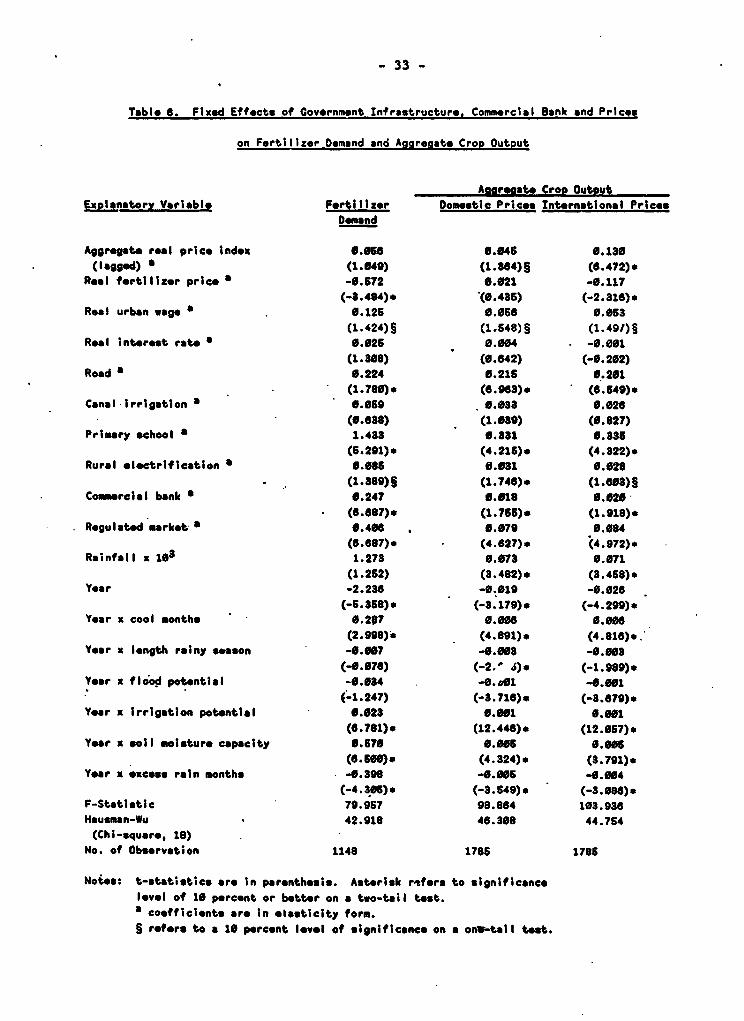
VII. Determinants of Fertilizer Demand and Aggregate Crop Output

For fertilizer demand and output supply the fixed effects model

has to be used. The measured permanent district characteristics are

therefore not sufficient to fully characterize the endowment of a district.

Fertilizer demand is seen to decline significantly when the price of

fertilizers is increased (elasticity of -0.57) and to increase when the

urban wage rises (elasticity of 0.13). This effect is statistically

significant if the appropriate one-tail test is used, as it makes no sense

to expect a negative sign here. In contrast, we see a perverse positive

interest elasticity, but the effect is.not statistically significant.14 A

positive interest rate effect may indicate that there is still an

14/ Since a positive sign expectation makes no-economic sense in this casea one-tail test is inappropriate.

- 32 -

unresolved simultaneity problem with respect to this variable if government

responds to higher demand for fertilizers by increasing the rate of

interest. Fertilhzer demand increases with all infrastructure investments,

although effect of canal irrigation is not significant. The effects of

primary schools, regulated markets and commercial banks are particularly

large and precisely estimated.

These extremely clear results accord fully with what is known fromi

other studies of the growth of fertilizers. To the previous literature

they add the first estimates of the impact on fertilizer demand of changes

in the rural bank network.

Finally the agroclimate x time interactions accord -very well with

what what is known about the influence of agroclimatic endowments on the

potential of green revolution technologies, with fertilizer demand growing

especially fast in green revolution areas with cool months, irrigation or

high soil moisture capacity, while being held back in areas of excessively

high rainfall and poor water-control.

In order to illustrate the endogeneity problem of using domestic

prices in explaining aggregate crop output we present results with both the

domestic and the international price indices. The comparisons clearly show

that an endogeneity problem is being circumvented when prices are

instrumented via the international price indeX. The coefficient of the

domestic price is only 0.06 while that with the international price is

0.24. Moreover, the aggregate crop supply elasticity of 0.13 estimated

with the international price exceeds the elasticities estimated for India

in BBQ and that estimated for the world in BYBM by a factor of 1.5 to 2.

- 33 -

Table Fixed Effects of covornmont Infrastructure. Commercial Bank and Prices

on Fertilizer Demand and Aggregato Crop Output

Aspreast. CrOp OutputExplanatory Variable Fertilizer Domestic Prieos International Prices

Demand

Aggregate roal price index 0.068 9.046 0.130(lagged) a (1.649) (1.884)§ (6.472)*

Real fertilizer price a -0.572 0.021 -0.117(-3.484)o (0.486) (-2.316)o

Roal urban wage a 0.125 0.056 0.063(1.424)§ (1.548)§ (1.491)§

Real interest rate 0.025 0.004 * -O.W1(1.308) (0.642) (-0.202)

Road a 0.224 0.216 0.201* ~(1.789). (6.968). (6.549).

Canal irrigation 0.069 0.03a 0.026(0.638) (1.039) (0.827)

Primary school a 1.433 * .881 0.835(6.291)* (4.216)- (4.322)*

Rural electrification a 0.0865 .031 0.028(1.889)§ (1.746). (1.693)§

Comercial bank a 0.247 0.018 0.020-(c.6e7)0 (1.766). (1.918)*

Regulated "rket * 0.406 0.079 0.O84(6.687). (4.627). (4.972)*

Rainfall x 193 1.273 0.073 0.071(1.252) (3.482). (3.468)*

Year -2.236 -0.019 -0.026(-6.358). (-3.179)* (-4.299)*

Year x cool months 0.207 0.008 0.090(2.998). (4.891)* (4.816)*.

Year x length rainy season -6.097 -. 003 -9.99(-9.976) (-2. 4).* (-1.989).*

Year x flood potential -0.084 -0. D1 -0.001

(-1.247) (-3.716)* (-3.679).Year x irrigation potential 0.023 0.001 0.001

(6.781)* (12.440)e (12.OS7)*Year x soil moisture capacity 0.57a 0.006 0.006

(6.600). (4.324). (3.791).Yoer x excose rain months -0.398 -. W05 -0.W04

(-4.306)s (-3.649)* (-3.086)*F-Statistic 79.967 98.864 103.936Hausman-Wu 42.918 46.308 44.764(Chi-square, 18)

No. of Obsorvation 1148 1785 1786

Notes: t-statistice are in parenthesis. Asterisk r0fore to significancelevel of 10 percont or better on a two-tail test.a coefficients are in elasticity form.§ refors to a 10 percent level of significanco on a onw-tail test.

- 34 _

Nevertheless, the classic result of the aggregate supply elasticity

literature is reconfirmed: short-run aggregate crop supply elasticities are

small and do not exceed a level of 0.2.13

The endogeneity problem with the output price also affects the

estimation of the fertilizer price elasticity. Using the domestic output

price the fertilizer price does not appear to affect aggregate output. In

the specification using international output prices the fertilizer price

elasticity is negative (-.12) and statistically significant. The results

are consistent with BYBM (1986) and BBQ (1984). The remaining discussion

will therefore only consider the results with the international price.

Increasing real interest rates of the cooperative sector reduces

aggregate output marginally an elasticity of about -0.001, while increasing

the density of commercial banks tends to increase crop output with an

elasticity of 0.020. The expansion of financial institutions thus seems to

exert a direct impact on aggregate crop output and a larger effect in

fertilizer demand as. well as on some of the private agricultural

investments.

Except for irrigation, all other infrastructure variables affect

aggregate crop output positively. The overwhelming impact of

infrastructure on aggregate crop output found in BYBM for international

13/ We attempted to estimate the long-run aggregate elasticity of supplywith this data set, using a free form lag structure of five pastprices. The sum of the coefficients was .28, and we could not, withthis technique, estimate a larger long-run aggregate supply response.However, long-run supply responses must be-larger, as discussed inBYBM.

- 35 _

data is thus confirmed in this Indian study. Quantitatively the effects o-

primary schools and roads are the largest, with elasticities of 0.34 and

0.20 respectively. BYBM found large effects for education as well. They

also found large irrigation effects but irrigation in the BYBM study

include both private and canal irrigation.

As expected residual growth of output (after account is taken of

prices, interest rates, infrastructure and banks) was larger in areas with

good irrigation potential, high soil moisture capacity, and cool winters.

It was lower in areas with excess rain and in areas liable to flooding.

VIII. Discussion

In the paper we have successfully demonstrated that with

appropriate panel data it is possible to overcome simultaneity and

unobservable variable problems arising from the joint dependence of the

decision of farmers, financial institutions and government agencies-on

location and agroclimatic factors of the region within they operate. It

then becomes possible to explain in an integrated fashion how the decision

of these actors interact and ultimately affect agricultural investment and

output. In addition, by judiciously using international prices we have

shown that it is possible to overcome simultaneity problems which have long

plagued the analysis of aggrogate supply response to output prices.

The reduced form regressions of infrastructure, banks, investments

and output on agroclimatic and location characteristics show the

overwhelming importance these factors which must have had over the history

of these districts on all decision-makers in the system. The importance of

- 36 -

the interaction terms with time shows that the agroclimate factors have

continued to govern the rate at which districts can take advantage of new

agricultural opportunities and have continued to govern public, bank and

private investuent allocation decisions over the period analyzed.

For the first time this paper presents results on the effect of

the expansion of financial intermediation on agricultural investment and

output .which are not seriously flawed because they ignore fungibility of

financial resources or the other econometric problems discussed above. The

expansion'of the commercial banks into rural areas had a large'effect on

fertilizer consumption and on fixed private investment. It also affects

output, but with an elasticity of only 0.02. In order to see how much the

bank expansion has contributed we tabulate in table 7 the estimated impact

of all independent variable, on the dependent variables in the decade of

the'1970s. These estimates are the percentage change in the dependent

variable caused by the changes in the independent variable, estimated as

the product of the change in the independent variable times the regression

coefficient which is divided by the average value of the dependent

veriable. Here we can see the contributions of different factors to growth

of dependent variables over the decade, 1971-1981. Obviously the effects

of a particular variable will be small if it did not change much over the

decade, irrespective of its potential impact as measured by the regression

coefficient.

The rapid Bank expansion increased fertilizer demand by about 23

percent, investment levels in tractors by 13 percent, investment in pumps

by 41 percent, milk animals by 46 percent, and in draft animals by about 38

percent. They also increased the aggregate crop output by nearly 3

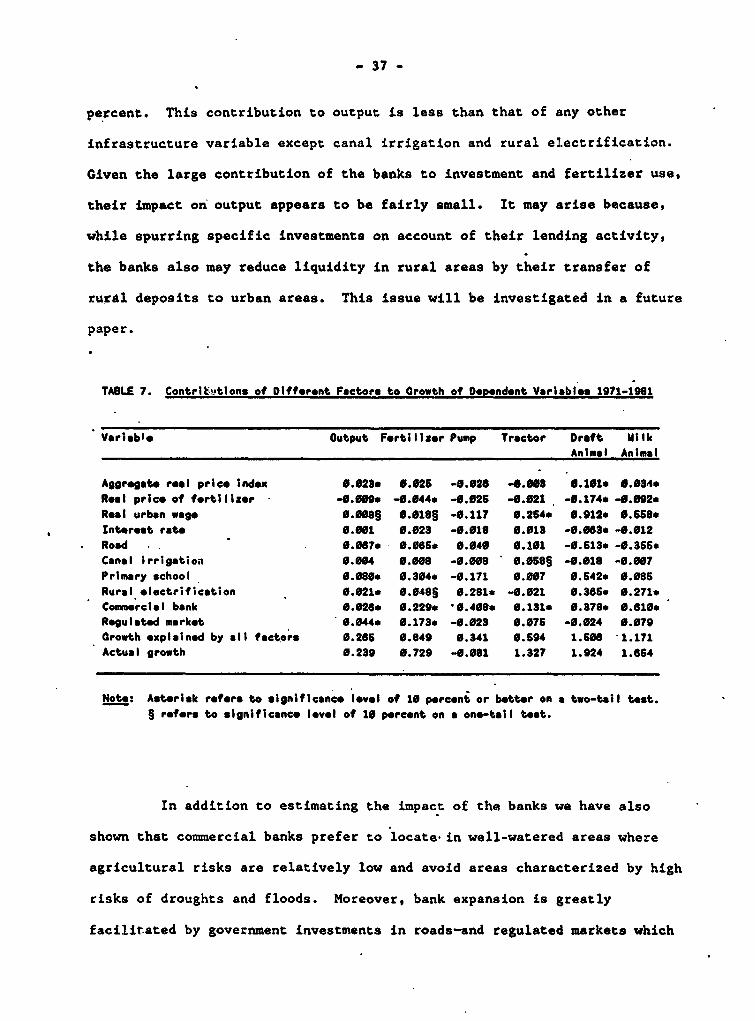
- 37 -

percent. This contribution to output is less than that of any other

infrastructure variable except canal irrigation and rural electrification.

Given the large contribution of the banks to investment and fertilizer use,

their impact on output appears to be fairly small. It may arise because,

while spurring specific investments on account of their lending activity,

the banks also may reduce liquidity in rural areas by their transfer of

rural deposits to urban areas. This issue will be investigated in a future

paper.

TABLE 7. Contrit!,t.ions of Difforent Factor. to Growth of Dependent Variables 1971-1991

Variable Output Fertillzer Pump Tractor Draft MilkAnimal Animal

Aggregat. real price index 0.023* e.o25 -9.026 -. 008 6.161* o.084*Real price of frtilIlzer -0.009* -. 044* -0.02 -0.021 -0.174* -0.092.Real urban wage 0.009§ 0.018§ -0.117 0.254* 0.912* 0.558.Interest rato 0.001 0.028 -0.018 0.01 -0.083* -0.012Road 0.0687 0.06* 0.0.40 0.101 -6.513* -0.356*Canal irrigation O.6Z4 O.68 -0.008 0.058§ -0.018 -0.007Primary school 0.080* 0.304* -0.171 0.007 0.642. 0.086Rural electrification 0.021* 0.048§ 0.281* -0.021 0.385S 0.271*Commercial bank 0.626. 0.229.* 0.408. 0.131. 0.878* 0.610*Regulated market 60.44* 0.17. -0.028 0.075 -0.024 0.079Growth explainod by all factors 0.266 0.849 0.341 0.594 1.66 1.171Actual growth 0.239 6.729 -0.081 1.327 1.924 1.664

Not.: Asterisk refers to significance level of 16 percent or better on a two-tail test.§ refers to significance lovel of 10 percent on a one-tall teot.

In addition to estimating the impact of the banks we have also

shown that commercial banks prefer to locate in well-watered areas where

agricultural risks are relatively low and avoid areas characterized by high

risks of droughts and floods. Moreover, bank expansion is greatly

facilitated by government investments in roads-and regulated markets which

- 38 -

enhance the liquidity position of farmers and reduce transaction costs of

both bank and farmers.

Our estimates of interest elasticity of investment while

econometrically a bit less secure than the effect of bank expansion,

suggest that changes in real interest clearly reduce some of the long-term

private investments. On the other hand, we are unable to show an impact of

interest rates on either fertilizer demand or aggregate output, i.e. the

impact of higher interest rates on reducing investment in long-term assets

is not sufficiently large to have a perceptible impact on output. And for

short-term credit used to buy fertilizer it appears that availability of

credit (as measured by the bank network) is clearly more important than the

interest rate.

In the reduced form cross-sectional regressions regions with high

irrigation potential have larger population density, better infrastructure,

a more developed banking system, higher private investment rates and higher

aggregate crop output. They are also favored in the allocation of new

infrastructure and are preferred by banks. They are also able to banefit

more from new technology in terms of fertilizer demand, investments and-

output. On the other hand, the analysis of the government's own

additional investment in irrigation between 1961 and 1981 suggest positive,

but barely statistically significant, impact of these irrigation

investments on Bank expansion, tractor investment and crop output. As

table 7 shows the estimates imply a near zero contribution of canal

irrigation to aggregate crop output over the 1970s. In order to understand

this puzzle it is important to recall that the measure of irrigation

potential must include both the already developed as well as the yet to be

- 39 -

developed potential. There is therefore collinearity between past

investment in canal irrigation and potential and the reduced form effects

of irrigation potential include the effects of the past investments. The

fixed effects analysis over time, however, looks only at the impact of the

additional government investment over the period. Therefore finding a low

impact of recent government investments is not inconsistent with high

Impact of past investment. This would be especially the case if the rate

of return to new canal irrigation had been declining over time as the best

sites for irrigation became progressively exhausted. Moreover the estimates

do not measure the impact of the very important private investment in

irrigation.14 The findings therefore do not imply that private investment

in irrigation had a low return, an issue which cannot be analyzed with the

techniques utilized. Canal irrigation investment in the 1960s and 1970s

was insignificant compared to private investment. Over the 21 years

analyzed, area irrigated by the government (canal) increased from 58 ha to

75 ha per 1000 ha of geographic area. Area irrigated by wells, i.e.

privately increased much-more rapidly from 54 ha to 114 ha per 1000 ha of

geographic area, i.e. private additions to irrigation exceeded government

additions by a factor of nearly 4 to 1.

Improved road investment has been shown to enhance agricultural

output with an elasticity of about 0.20. In the 85 sample district roads

have on average increased by 40 percent between 1971 and 1981. Roads would

thus have contributed directly 7 percent each to the growth of agricultural

14/ These results are not altered if the canal irrigation variable isreplaced by the public irrigation, i.e. ineluding the area under tankswhich has been declining.

-40-

output and fertilizer use over this period. We have seen above that they

have also contributed to bank expansion. On the other hand, for given bank

density and other infrastructure, the direct effect of roads on private

investment is mixed, suggesting that tho major effect of roads is not via

their impact on private agricultural investment but rather on marketing

opportunities and reduced transaction costs of all sorts.

Regulated markets have an elasticity with respect to output of

0.08. They have expanded rapidly after 1969 and the growth (87 percent)

during this period would have contributed nearly 4 percent to agricultural

output and 17 percent to the demand of fertilizers. As in the case of

roads, the markets also have little effect on the private investments, i.e.

their effect works directly on output supply decisions.

In contrast electrification has a clear impact on inveatment in

fixed capital, especially on pumps where it has contributed an increase of

28 percent to investment levels. Via these investments and klso via

fertilizer demand (about 5 percent increase) electrification has increased

output over the decade by about 2 percent.

Finally primary education has added 8 percent to crop output over

the decade, a very large effect indeed. This has come about primarily via

a nearly 30 percent increment to fertilizer demand.

In terms of prices the study confirms that short run aggregate

crop supply elasticities are inelastic even once simultaneity problems

which have plagued this literature are overcome. In addition it shows that

output prices, fertilizer prices and urban wages can have substantial

- 41 -

impacts on private fixed capital investments even in the long run, as the

lagged prices in these equations refer to prices ruling in the previous

intercensal period, i.e. 5 years earlier on average. The results suggest

that wages increases tend to lead to increased private investment while

fertilizer price increases tend to reduce investments. Thus for wages

substitution effects dominate the profitability effects while for

fertilizers the opposite is the case.

The agricultural development literature has been dominated by

schools which tended to emphasize the importance, or lack thereof, of

specific determinants of agricultural growth. Price fundamentalists have

been at odds with irrigation determinists. The 1970s and early 1980s have

been dominated by advocates of cheap sources of growth from agricultural

research and education. In World Bank projects road infrastructure and

market development have taken a backseat relative to the forced expansion

of cheap agricultural credit. Advocates of such agricultural credit have

been attacked by scholars emphasizing the virtues of savings and market-

determined interest rates. As the evidence in this paper suggests, reality

is far too complex to be put into such black and white terms. Prices

really do matter but so do infrastructure, markets, and banks.

_ 42 -

References

Bapna, S.L., H.P. Binswanger and J.B. Qu$zon, 1984, "Systems of OutputSupply and Factor Demand Equations for Semi-Arid Tropical India.",Indian Journal of Agricultural Economics, 39, 179-202.

Barnes, D.F., and H.P. Binswanger, 1986, "Impact of Rural Electrificationand Infrastructure on Agricultural Changes, 1966-1980," Economicand Political Weekly, 21, 26-34.

Binswanger, H.P., 1974, "The Measurement of Technical Change Biases withMany Factors of Production", American Economic Review, 64,964-976.

Binswanger, H.P., and M.R. Rosenzweig, 1986, 'Behavioral and MaterialDeterminants of Production Relations in Agriculture," Journal ofDevelopment Studies, 21,-503-539.

Binswanger, H.P., M. Yang, A. Bowers and Y. Hundlak, 1987, "On theDeterminants of Cross-Country Aggregate Agricultural Supply,"Journal of Econometrics, 36, 111-131.

Boyce, J.K., and R.E. Evenson, 1975, National and InternationalAzricultural Research and Extension Programs, New York:Agricultural Development Council.

Evenson, R.E., and Y. Kislev, 1975, Agricultural Research and Productivi:v,New Haven: Yale University Press.

Lau, L.J., and P.A. Yotopoulos, 1987, "The Meta-Production FunctionApproach to Technological Change in World Agriculture," Journal ofDevelopment Economics, (forthcoming).

Mundlak, Y., 1985, The Aggregate Agricultural Supply, Working Paper No.8511 (Center for Agricultural Economic Research, Rehovat).

PPR Working Paper Series

Title Author Date Contact

WPS144 Product Differentiation and the

Treatment of Foreign Trade InCGE Models of Small Economies Jalme de Melo February 1989 K. Cabana

Sherman Robinson 61539

WPS145 Revenue Raising Taxes: General

Equilibrium Evaluation of AlternativeTaxation In U.S. Petroleum Industries Jaime de Melo February 1989 K. Cabana

Julie Stanton 61539

David Tarr

WPS146 Exchange Rate-Based Disinflation, Wage

Rigidity, and Capital Inflows:Tradeoffs for Chile 1977-81 Timothy Condon February 1989 K. Cabana

Vittorlo Corbo 61539

Jaime de Melo

WPS147 The Private Sector's Response to

Financial Liberalization In Turkey:1980-82 Izak Atlyas January 1989 W. Pitayatonaka

60353

WPS148 Impact of the International CoffeeAgreement's Export Quota System on theWorld Coffee Market Takamasa Akiyama February 1989 D. Gustafson

Panayotis N. Varangis 33714

WPS149 Reflections on Perestroyka and theForeign Economic Ties of the USSR Bela Balassa January 1989 N. Campbell

33769

WPS150 Improving the Currency Composition

of External Debt: Applications In

Indonesia and Turkey Ken Kroner January 1989 L. Chavarria

Stijn Claessens 33730

WPS151 U.S. Trade Policy TowardsDeveloping Countries Bela Balassa January 1989 N. Campbell

33769

WPS152 Subsidies and Countervailing Measures:

Economic Considerations Bela Balassa January 1989 N. Campbell

33769

PPR Working Paper Series

Title Author Date Contact

WPS153 An Analysis of Debt Reduction SchemesInitiated by Debtor Countries Ishac Diwan March 1989 L. Chavaria

StiJn Claessens 33730

WPS154 Forecasting, Uncertainty and Public

Project Appraisal Jock R. Anderson February 1989 A. Kltson-Walters

33712

WPS155 Measuring Adult Mortality In

Developing Countries: A Review and

Assessment of Methods Ian Timaeus

Wendy Graham

WPS156 Credit Cooperatives in Israeli

Agriculture Yoav Kislev March 1989 C. Spooner

Zvi Lerman 37570

Pinhas Zusman

WPS157 A Policy Model for Tunisia with

Real and Financial Flows Martha de Melo January 1989 A. Bhalla

Marc Leduc 60359Setareh Razmara

WPS1S8 Labor Redundancy In the TransportSector Alice Galenson February 1989 W. Wright

33744

WPS159 Current International Gas Trades

and Prices Kay McKeough March 1989 M. Fernandez

33637

WPS160 Evaluating the Performance of Public

Enterprises in Pakistan Mary M. Shirley March 1989 R. Malcolm61708

WPS161 Commodity-indexed Debt in

International Lending Timothy Besley March 1989 J. Raulin

Andrew Powell 33715

WPS162 Ups and Downs In Inflation: Argentina

Since the Austral Plan Miguel A. Kiguel

WPS163 The Impact of Infrastructure and

Financial Institutions on AgriculturalOutput and Investment In India Hans P. Binswanger March 1989 J. Arevalo

Shahidur R. Khandker 30745

Mark R. Rosenzweig