Titel der Arbeit:

How Labor Market FrictionsMatter for

Financial Decision Making

Schriftliche Promotionsleistung zurErlangung des akademischen Grades

Doctor rerum politicarum

vorgelegt und angenommen an derFakultat fur Wirtschaftswissenschaft

Otto von Guericke Universitat Magdeburg

Verfasser: Konstantin Wagner, M.Sc.Geburtsdatum und -ort: 19.05.1989, Bamberg

Arbeit eingereicht am: 31.12.2020

Gutachter der schriftlichenPromotionsleistung: Prof. Michael Koetter, PhD

Prof. Dr. Felix Noth

Datum der Disputation: 26.04.2021

How Labor Market FrictionsMatter for

Financial Decision Making

Preface

Human beings do not act in isolation. This particularly holds for economic systems

in which workers are employed at firms. In one of the seminal papers in economics,

Coase (1937) identifies transaction costs to be the prime economic reason why firms are

formed to organize production, and, consequently, transaction costs also explain why

workers are employed at firms. At first glance, this appears to be a subtle detail on the

organization of economic activity. It has, however, a huge impact on individuals, as

this subtle detail also is the reason why the provision of their workforce in the economy

is performed through employment at firms.

In a free and capitalist society, markets constitute the ecosystem of firms. Firms

obtain their resources in factor markets and financial markets, while produced goods

are sold via product markets. In the four papers of this thesis, I—together with my

co-authors—study the interrelation of these ecosystems with particular focus on labor

markets from a corporate finance angle. Each of the papers highlights different aspects

in the employment of labor by firms. In Paper 1 I study labor rigidities and their

impact on firm financial performance, in Paper 2 we evaluate behavioral effects due

to changes in compensation structure, in Paper 3 we investigate pay differences along

task-related differences in marginal returns to talent, and in Paper 4 we study cross-

sector mobility of former bankers that moved to banking supervision. These aspects

do not only matter for financial decision making but also come with implications for

the economy as a whole.

The economic literature on labor is traditionally interested in labor markets, namely

in how prices and quantities in labor markets come about and how these translate into

wages, employment and, more recently, income distribution. Financial economics is

traditionally interested in financial markets, i.e., how firms attain funding, and finan-

cial performance, i.e., how firms’ economic activity can ensure to provide goods and

i

Preface ii

services in an economically sustainable manner. Recently, financial economists also

focus on the interrelation of labor and finance within and across firms. One reason for

this is that labor is different from other factors of production in various aspects. These

differences have important implications on firm financing, but can also retroactively

affect the greater economy. Another reason is that well-established figures on labor

markets recently observed new trends. Three prominent examples are the decrease

in labor shares (e.g. Karabarbounis and Neiman, 2014; Dao, Das, Koczan, and Lian,

2017), job-market polarization in developed economies (e.g. Autor, Katz, and Kearney,

2006; Goos and Manning, 2007), and the stark increase in top-level pay (e.g. Rosen,

1981; Gabaix and Landier, 2008). For a sound understanding of these phenomena, the

firm-centric perspective of financial economists is of great value. Not only can corporate

structures be sources of such patterns, they will also be affected by them in a plethora

of ways. All papers in this thesis have in common that they relate to meaningful trends

in labor markets. To enlighten the discussion on these, the papers trace stylized facts or

common narratives on labor markets back to their origin at the firm level (Paper 1 and

Paper 3) or even at the level of individual employment contracts (Paper 2 and Paper 4).

When investigated separately, both the combination of production factors and fi-

nancing activities of firms can be well described by means of traditional tools that

economists use, such as production functions and firm financial analyses. Not surpris-

ingly, these tools are regularly applied in the fields of labor economics and financial

economics, respectively, to investigate the ecosystems of interest. However, to study

interaction effects between labor and finance empirically, conventional means do not

suffice most of the time. For instance, while survey data offers great insight into

individual decision making, labor income, and information on many covariates, it is

regularly hard—if not impossible—to link such data to firm financials. At the same

time, the best data on firm financials is useless if it offers no insights into the specific

characteristics of the labor force employed in firms. The papers of this thesis therefore

do not only rely on firm financials and financial market data, but rather combine those

data with granular information on labor markets and employment. As such, the papers

of this thesis can contribute to the evaluation of the impact of labor on various levels.

As economists can seldom execute controlled field experiments to test their conjec-

tures, it is of utmost importance to understand the context from which the empirical

results are sourced. Henceforth, while the availability of data is key to establish cer-

Preface iii

tain empirical facts, it is econometric analyses that allow one to uncover meaningful

regularities of economic ecosystems well below the surface of a pure statistical descrip-

tion. In some cases, an empirical setting might be suitable to argue that variation in

explanatory variables is sufficiently exogenous to interpret estimated coefficients in a

causal way (I do so in Paper 1). It is very important to understand, however, that it is

not the mechanical application of a model, but rather the investigation of the specific

features of a settings, that allows such inference. In the real world, the researcher will

find herself in less optimal situations most of the time (Paper 2, Paper 3, and Paper 4).

However, econometric anaylses may still be informative in the absence of “clean” iden-

tification. For instance, in Paper 2 we argue that while the regulatory shock that we

investigate clearly is a shock to compensation structure, its exogenous nature is unclear

and, subsequently, needs to be studied in depth. Therefore, the econometric analyses

in Paper 2 do not solely rely on a mechanical application of the difference-in-differences

approach, but rather on the profound description of the institutional setting, in tests

that falsify confounding events, and in controlling for alternative explanations.

There is a clear trend towards more reliance on empirical research rather than pure

theoretical, i.e., model-based, research. Note, however, that the two approaches are

highly related. The motivation to work empirically is largely motivated by theoretical

work and vice versa. In many cases, empirical studies inspired theorists to rethink

their way of modeling the behavior of economic agents (e.g. Kahneman and Tversky,

1979). In other cases, it took empiricists a long time to ultimately be able to provide

evidence that backed well-established theoretical work. One prominent example is the

provision of empirical evidence by Aggarwal and Samwick (1999) on the principal-agent

model of executive compensation. Also, it can often be a first step to provide empirical

evidence in line with a plausible theory on a subject (Paper 3), rather than rejecting

research ideas that do not offer fully fledged causal identification strategies. Clearly,

such evidence cannot be regarded as the ultimate empirical proof. It can, however,

inform ongoing debates on important issues by revealing patterns and by putting them

into perspective by directly relating it to theory.

Labor market-related topics are usually dealt with in a highly emotional way in

the public, as most people are directly affected by labor-market outcomes. Therefore,

it is of first order importance to support policy makers with scientific evidence to

support their decision making. With two of my papers I shed light on topics that are

Preface iv

particularly sensitive—financial costs of fixed wages and incentive pay of bankers. First,

in Paper 1 I demonstrate that while safe contracts might be favorable to workers in the

short run, they might come at some cost in the long run. I show that the decrease in

financial performance that firms experience in times of competitive pressure is mostly

related to labor leverage due to rigid labor costs. If both the inflexibility of wages and

the competitive pressure persist, it is likely that firms have to be restructured and,

ultimately, workers might be laid off. I do not claim that workers should get equally

flexible claims as residual claimholders in order to permanently strengthen firm financial

results. For policy makers it is important, however, to see the financial implications of

rigid labor costs when making policy decisions with respect to labor. One such example

is the introduction of short-time working plans like the German Kurzarbeitergeld. This

temporary measure allows firms to decrease labor leverage while retaining its workforce.

Second, we investigate the effects of a policy intervention on banker’s pay in Paper 2. It

is well-established that mis-aligned compensation practices played a role in the financial

crisis of 2007-2009 (e.g. Efing, Hau, Kampkotter, and Steinbrecher, 2015). The brute-

force approach of the EU banker bonus cap—that might have largely been motivated

by emotions rather than consultations of experts on the matter—is unlikely to realign

bankers’ incentives. We document that compensation contracts after the introduction

of the EU banker bonus cap offered higher levels of fixed pay, implying more insurance

to bankers against their own poor performance. Consistently, we find no evidence on

decreased risk-taking—which was the policy’s goal—but even increases in some of the

risk-measures we investigate.

Bibliography

Aggarwal, R. K., and A. A. Samwick. 1999. The Other Side of the Trade-Off: The

Impact of Risk on Executive Compensation. Journal of Political Economy 107:65–

105.

Autor, D. H., L. F. Katz, and M. S. Kearney. 2006. The Polarization of the U.S. Labor

Market. American Economic Review 96:189–194.

Coase, R. 1937. The Nature of the Firm. Economica 4:386–405.

Dao, M. C., M. Das, Z. Koczan, and W. Lian. 2017. Why Is Labor Receiving a Smaller

Share of Global Income? Theory and Empirical Evidence. IMF Working Paper No.

17/169.

Efing, M., H. Hau, P. Kampkotter, and J. Steinbrecher. 2015. Incentive Pay and

Bank Risk-Taking: Evidence from Austrian, German, and Swiss Banks. Journal of

International Economics 96:123–140.

Gabaix, X., and A. Landier. 2008. Why has CEO Pay Increased so Much? Quarterly

Journal of Economics 123:49–100.

Goos, M., and A. Manning. 2007. Lousy and Lovely Jobs: The Rising Polarization of

Work in Britain. Review of Economics and Statistics 89:118–133.

Kahneman, D., and A. Tversky. 1979. Prospect Theory: An Analysis of Decision under

Risk. Econometrica 47:263–292.

Karabarbounis, L., and B. Neiman. 2014. The Global Decline of the Labor Share.

Quarterly Journal of Economics 129:61–103.

Rosen, S. 1981. The Economics of Superstars. American Economic Review 71:845–858.

v

Paper 1:

Competition, Cost Structure, and

Labor Leverage: Evidence from the

U.S. Airline Industry

Competition, Cost Structure, and Labor Leverage:

Evidence from the U.S. Airline Industry∗

Konstantin Wagner†

This Draft: December 29, 2020

First Draft: April 4, 2019

Abstract

I study the effect of increasing competition on financial performance throughlabor leverage. To capture competition, I exploit variation in product marketcontestability in the U.S. airline industry. First, I find that increasing compet-itive pressure leads to increasing labor leverage, proxied by labor share. Thisexplains the decrease in operating profitability through labor rigidities. Second,by exploiting variation in human capital specificity, I show that contestabilityof product markets induces labor market contestability. Whereas affected firmsmight experience more stress through higher wages or loss of skilled human capi-tal, more mobile employee groups benefit from competitions through higher laborshares.

JEL Classification: G39, J31, L93

Keywords: Competition, labor leverage, labor share, threat of entry

∗I am grateful to Jeff Gorham from the U.S. Department of Transportation for helping me withthe data. I thank Mario Brandtner, Stefano Colonnello, Michael Koetter, Thomas Krause, WilliamMcShane, Matthias Mertens, Carola Muller, Steffen Muller, Felix Noth, Paige Ouimet, GianpaoloParise, Gregor von Schweinitz, Jessie Wang, Qizhou (Leo) Xiong, Yishay Yafeh, seminar participantsat the IWH, and the IWH Financial Markets & SAFE Winterschool (Riezlern) for insightful discussionsand comments. Felix Klischat and Sithara Thies provided excellent research assistance.†Otto-von-Guericke University Magdeburg and Halle Institute for Economic Research (IWH),

Kleine Markerstraße 8, D-06108 Halle (Saale) Germany. Phone: +49 345 7753 755. E-mail:konstantin.wagner@iwh-halle.de.

1 Introduction

Evaluating the effects of competitive pressure on firms is key to understand an econ-

omy’s ability to adapt to a changing economic environment. At the firm level, com-

petitive shocks often materialize as contractions in revenues. How hard these shocks

hit firms depends on how flexibly they can react to such adverse events. Operating

leverage—the ratio of fixed to total costs—expresses the sensitivity of a firm’s income

to changes in revenues. Consequently, firms with high operating leverage will suffer

more from a negative demand shock than firms that can easily adapt to a changing

economic environment.

In the presence of labor rigidities, labor expenses contribute to labor leverage, a

crucial component of operating leverage. The labor share, which captures the fraction

of output that goes to labor, has been used in the finance literature as a measure of

labor leverage (Marfe, 2017a; Donangelo, Gourio, Kehrig, and Palacios, 2019). This

paper investigates how economic shocks driven by competitive pressure affect firm

performance and how these relate to labor leverage. By capturing competitive pressure

through threat of entry, I address endogeneity concerns associated with decisions of

entry (e.g., Goolsbee and Syverson, 2008; Parise, 2018).

Whereas labor leverage is sensitive to both competition in product markets and

labor markets, prior studies have neglected the latter aspect of contestability. My

testing ground provides a comprehensive assessment of the interplay between com-

petitive pressure and labor leverage. More specifically, I study the effects of product

market contestability and whether product market contestability induces labor market

contestability.

To investigate firm-level competition, I focus on the U.S. airline industry. The

distinctive setting allows me to study the effects of competition on firm-level labor

shares and performance. The U.S. airline industry is characterized by high competitive

pressure and frequent entries of competitors into spatially segmented markets. Using

highly granular data on air carriers, I am able to assess competition at the route-market

level.

I identify the effect of competitive pressure on firm profit margins by exploiting the

threat of entry by a budget carrier. On the level of route markets, I find that incumbent

airlines decrease ticket prices by -2.1% on average, once a market becomes contestable.

This leads to a decrease in incumbents’ size by -5.5% on average, as proxied by ticket

sales in a market. Second, I show that the firm-level labor share of incumbents is

1

positively related to both realized entry and threat of entry. That is, a higher fraction

of total revenues is spent on wages, once competitive pressure on airlines increases.

Third, I decompose the labor share in different ways to illustrate how lower operating

profitability is directly linked to increases in labor leverage. Whereas the share of

non-labor related expenses instantly adjusts to competitive pressure, the share of labor

expenses, i.e., the labor share, increases. This result is economically significant. I find

that more than 80% of the decrease of an airline’s EBIT margin caused by competitive

pressure is related to the increase in labor leverage.

I provide evidence that the labor shares of different groups of employees are differen-

tially affected by competitive pressure. Management compensation does not contribute

to increases in the labor share. One explanation of this result might be lower levels

of variable pay at times of tougher competition owing to weaker financial performance

of incumbent airlines. This is in line with a narrative that variable compensation is

a risk-sharing contract and as such allows firms greater flexibility at times of poorer

economic performance (e.g., Efing, Hau, Kampkotter, and Rochet, 2018). In contrast,

both ground crews and flight crews benefit from more competition. The results for the

latter group can partially be attributed to labor market effects. This is consistent with

labor market contestability induced by product market contestability.

In the empirical analysis, I use a measure of human capital specificity to investigate

whether product market contestability can induce labor market contestability. If an

entry into a product market becomes more likely, the entering firm will also demand

more labor and thus contestability of related labor markets will increase, too. Oligop-

sonists’ rents will be challenged in a similar way as those of oligopolists. Additional

pressure on labor markets can increase operating leverage through higher wages, which

potentially crowds out financing opportunities. At the same time, contestability of

labor markets could induce a loss of skilled human capital through poaching.

There is a growing body of literature on how labor rigidities affect financing condi-

tions of firms. For instance, Marfe (2017b) demonstrates how the labor share—a proxy

of labor leverage—can explain the premia of value firms over growth firms. In addi-

tion, Marfe (2017a) argues that income insurance from shareholders to workers comes

at the expense of higher short-run dividend risk. Donangelo et al. (2019) document

that firms with higher labor leverage exhibit higher equity returns. These returns come

at the cost of a higher sensitivity to economic shocks. Simintzi, Vig, and Volpin (2015)

show that higher levels of labor protection—which make labor expenses arguably more

rigid—increase operating leverage, crowding out financial leverage. This is in line with

2

Favilukis, Lin, and Zhao (2019) who find that higher operating leverage through higher

labor shares leads to higher credit risk. I contribute to this literature by showing that

the deterioration of firms’ operating performance from competitive pressure is linked

to changes in labor leverage. My results support the narrative that rigid labor costs

lead to increases in a firm’s sensitivity to adverse sales shocks through operating lever-

age. More specifically, the lower ability to turn revenues into profits, i.e., lower EBIT

margins caused by labor rigidities in my setting, narrows firms’ abilities to finance

operations with retained earnings.

As a result of both its distinct competitive structure and regulated mandatory data

disclosure, the U.S. airline industry has been intensively researched in fields related to

industrial organization, competition and entry decisions (e.g., Berry, 1992; Borenstein

and Rose, 1994; Goolsbee and Syverson, 2008). More recently, the setting of the U.S.

airline industry has also been used to investigate pay determination on various levels

of corporations. For instance, Hirsch and Macpherson (2000) look at wages of airline

labor around deregulation, Benmelech, Bergman, and Enriquez (2012) investigate how

airlines in financial distress renegotiate wages, He, Whited, and Guo (2018) study how

relative performance evaluation in executive compensation affects competition, and

Aggarwal and Schenone (2019) exploit the availability of on-time performance data—a

key performance indicator for airlines—to evaluate the nexus between non-financial

performance and executives’ incentive schemes. I contribute to this literature by ex-

tending the analysis to airline-level labor shares and by investigating how competitive

pressure affects different labor groups differentially.

This paper is also related to the literature on the dynamics and determinants of

labor shares. Recently, researchers have found evidence of decreasing labor shares

for various developed economies (e.g., Karabarbounis and Neiman, 2014; Dao, Das,

Koczan, and Lian, 2017), contradicting the traditional view that the labor share is con-

stant (e.g., Kaldor, 1957). Explanations for this phenomenon are manifold and range

from a decrease in the cost of capital, increased trade and international outsourcing,

and the decline of labor market unionizations to measurement issues.1 Autor, Dorn,

Katz, Patterson, and van Reenen (2017) argue that firm heterogeneity in productivity

leads to industry concentration and ultimately lower labor shares. In their setting,

industry structure is driven by highly productive superstar firms. I investigate similar

regularities as Autor et al. (2017) but at the firm-level rather than the industry level.

1For a thorough description of potential drivers of the labor share, see Dao et al. (2017), forinstance.

3

Whereas the specific setting of the US airline industry allows me to observe increasing

competition rather than increasing industry concentration, I come to the same conclu-

sion. My findings verify the negative relation between market power and labor shares,

i.e., that a decrease (increase) in market power is related to an increase (decrease) in

labor shares.

More recently, we observe higher industry concentration, larger firms and fewer

competitors (e.g., De Loecker and Eeckhout, 2017), and job market polarization (e.g.,

Autor, Katz, and Kearney, 2006; Goos and Manning, 2007). In the light of these

developments, it is of particular interest to investigate the distribution of total revenues

among different groups of employees. Whereas the evolution of top-level pay has been

intensively researched in finance (e.g., Rosen, 1981; Gabaix and Landier, 2008), the

interest in within-firm pay inequality is new to this literature (e.g., Mueller, Ouimet,

and Simintzi, 2017; Dittmann, Montone, and Zhu, 2018a; Dittmann, Schneider, and

Zhu, 2018b). I contribute by examining how competitive pressure on firms affects

different groups of employees differentially and by documenting that especially mobile

labor groups benefit from this situation through higher labor shares.

2 The economics of labor share, operating leverage, and labor leverage

2.1 Measurement and interpretation

The labor share is the sum of labor costs over a measure of output. At the macro-level,

the labor share is usually defined as total labor compensation over gross domestic prod-

uct (e.g., Karabarbounis and Neiman, 2014). In this case, the labor share expresses the

fraction of the market value of final goods produced in a country going to wage-earners.

Hence, changes in the labor share capture the workforce’s time-varying participation

in national value-added through wages.

Firm-level studies often define the labor share as the fraction of labor expenses

over a firm-level measure of value-added (e.g., Marfe, 2017b; Donangelo et al., 2019).

The advantage of using value-added as the basis for firm-level labor shares is that the

macro-level labor share can be constructed through aggregation. Whereas the exclusion

of intermediaries omits double-counting, it neglects output of firms with high shares

of intermediary good production. As I do not provide a general equilibrium analysis, I

use total revenues as the basis of the calculation of labor shares, in line with the labor

share definitions of non-manufacturing sectors used by Autor et al. (2017).2 In this

2Estimations based on value-added in the appendix are based on the definition of value-added used

4

way, I capture the share of labor expenses relative to the gross output produced by

firms.

The concept of labor share is closely related to the concept of operating leverage.

Operating leverage captures the effect of changes in revenues on profits. The channel

of these changes is a firm’s cost structure, namely the relation of fixed costs to vari-

able costs. In the model of operating leverage, a higher share of fixed costs increases

profitability in times of high revenues, whereas it reduces profitability in times of low

revenues. This mechanism is analogous to financial leverage. High financial leverage

increases the positive impact of asset returns on equity returns in good times, but

also amplifies the negative impact in bad times.3 Operating leverage induced by labor

expenses is referred to as labor leverage (e.g., Lev and Zambon, 2003).

Marfe (2017a) uses labor share as a proxy for wage insurance from shareholders

to employees and shows that higher wage insurance can lead to higher short-term

dividend risk. The amplification of existing labor rigidities can have sizable effects on

firm performance. For instance, Simintzi et al. (2015) show that employment protection

has an impact on capital structure through the crowding out of financial leverage by

operating leverage. The work by Efing et al. (2018) confirms these findings. In their

study on the banking sector they show that banks with compensation plans that rely

more on variable components have lower operating leverage. At the same time, riskier

banks prefer to choose lower operating leverage.

The use of total revenues in the calculation of labor shares allows me to interpret

the labor share in the context of operating profitability. Based on accounting identities

of the profit and loss account, I decompose estimated effects on the EBIT margin

into the contribution of non-labor related expenses and of labor expenses, where the

latter is captured by the labor share. In this way, I can relate the estimated effects of

competitive pressure on profitability to different cost components, where labor share

can be interpreted as labor leverage, i.e., labor induced operating leverage.

2.2 Labor share and competition

In a simple model of oligopoly, a decrease in oligopolistic market power is followed by

a decrease in prices and an increase in aggregate quantities of goods sold. If product

by Favilukis et al. (2019).3Note that operating leverage is closely related to the concept of adjustment costs in production

with fixed costs (e.g., Lucas, 1967) or to situations where firms can only change production afterincurring additional adjustment costs (e.g., Hamermesh and Pfann, 1996).

5

market power is reduced by the entry of new firms, market shares of incumbent firms

will also decrease. In a first step, I therefore analyse the effects of competitive pressure

on ticket sales on distinct routes to determine the impact of competition in my setting.

More specifically, I estimate the price and quantity effects of competition both on

the total market and on the market subset, where only the incumbents’ tickets are

considered.

By construction, the labor share captures both competition in product markets

(revenues, denominator) and competition in labor markets (labor expenses, numera-

tor) in which firms operate. I therefore decompose the aggregate effect into its two

components to pin down the importance of each channel—product market competition

and labor market competition—in my setting.

Compared to a setting where there is perfect competition, uncontested labor mar-

kets are characterized by lower wages and a lower demand for labor. For instance,

Benmelech, Bergman, and Kim (2018) document that higher employer concentration

in local labor markets and lower wages go hand in hand. Following the idea of contesta-

bility, the expansion of a competitors’ activities should affect labor market outcomes.

Higher demand for labor and subsequently higher wages would then translate into

higher labor shares. Under the assumption of a perfect labor market, all firms would

be affected in the same way at a given point in time. It might be more realistic, how-

ever, to relax this assumption. Relaxations might be necessary because of regional

fragmentation, limited mobility of labor groups, or human capital specificity of em-

ployee groups across airlines. Differential affectedness of employee groups might thus

be explained by airline-employee group specific aspects that make the labor force of

some airlines more attractive to a potential entrant. In my empirical analysis, I apply

a measure of human capital specificity based on aircraft types employed by carriers. I

argue that airlines with matching human capital specificity would be affected more by

competitive pressure if contestability of labor markets is induced by product market

contestability.

3 The U.S. airline industry

3.1 Studying competition in the U.S. airline industry

One major challenge in studying the effects of competition is the definition of markets

and the identification of firms competing therein. This is particularly challenging when

considering differentiated multi-product firms or industries that are characterized by a

6

high level of market fragmentation (e.g., Hoberg, Phillips, and Prabhala, 2014; Hoberg

and Philips, 2016). The setting of the U.S. airline industry offers some special features

that help to deal with these challenges. First, flights are relatively homogeneous goods.

When compared, a connection between city A and city B by a legacy carrier and a

flight executed by a budget airline are close substitutes. The assumption of substi-

tutability is important, as I will use the threat of entry by a budget carrier to capture

competitive pressure. Homogeneity of goods is also underpinned by national regulation

and industry standardization of the U.S. carrier business. I show this substitutability

by investigating whether a budget carrier’s entry affects incumbent airlines’ quantity

and price decisions.

Second, a study of the U.S. airline industry has to consider the sub-markets in

which carriers operate. Spatial segmentation can be tackled by an analysis that takes

into account connections between regions. The U.S. airline data enables me to capture

precisely which airlines are competing with each other on routes between city markets.

In this way, I can evaluate a carrier’s exposure to competition.

Apart from the observability of the industry structure, an analysis of the U.S.

airlines has another benefit when it comes to investigating competition. The continuous

entry by budget carriers into the industry—and particularly the evolution of Southwest

Airlines’ business—is perceived as an industry-disrupting phenomenon. Budget airlines

are seen as one of the major reasons for the failure of the U.S. airline industry to be

profitable for decades (Borenstein, 2011). This makes it a suitable setting in which to

study tough competition at the firm-level.

3.2 Market penetration by Southwest Airlines

I focus on changes in competitive pressure which I capture by threat of entry at firm-

level to evaluate subsequent effects on labor shares of firms. Threat of entry is directly

linked to the concept of contestability. A market is said to be contestable if there

are no barriers that deter a potential competitor’s entry. According to the theory

of contestable markets, this alone is sufficient for competitive pricing of goods, even

without a single realized entry into the incumbents’ market (Baumol, Panzar, and

Willig, 1982). Early evidence from the literature on contestability suggests that airline

markets are in principle contestable: “once a carrier has a station at an airport it

appears to be relatively easy to start new service into that station” (Bailey and Panzar,

1981, p. 131).

7

In my analysis, I focus on changes in contestability that increase competitive pres-

sure on incumbent airlines. In order to evaluate the effect of competition, I look at

changes in contestability by considering changes in airline-level threat of entry. In de-

riving measures of competitive pressure at the airline level, I follow the approach of

Goolsbee and Syverson (2008), which is based on threat of entry by the budget carrier

Southwest Airlines.

The reasons for using threat of entry by Southwest Airlines for this study are

threefold. First, the airline industry is characterized by alliances and cooperation

between airlines, which makes identifying truly competing firms challenging. In this

respect, Southwest is different from other airlines in that it has not been involved in

code sharing or interline ticketing on national routes since its incorporation. Therefore,

Southwest can be considered a true competitor to other airlines.

Second, Southwest is not a budget airline that wins market shares by offering low

ticket prices accompanied by extra costs. Southwest is one of the leading carriers

in customer satisfaction, according to the Bureau of Transportation Statistics (BTS).

In an effort to ensure cost-efficiency and good on-time performance, Southwest has

developed its own boarding procedures to keep turnaround times short. In general,

low ticket prices are possible because of lean structures in the company. For instance,

to reduce complexity in training and route planning Southwest has kept to the Boeing

737 as the only aircraft type since the airline’s inception. Later in my analysis, I make

use of this feature when investigating the effects of contestability of product markets

on labor markets through human capital specificity.

Third, since the operation of its first flights in Texas in the 1970s, Southwest has

continued to expand its route-network all over the country, posing a severe threat to

the profitability of legacy carriers’ routes. As early as 1990 operating revenues from

domestic operations of Southwest corresponded to 12% of those of American Airlines

and increased steadily to 95% in 2010. In 2012, 2013 and 2014, Southwest Airlines’

operating revenues from domestic operations exceeded those of American Airlines.

4 Empirical approach

4.1 Threat of entry in airline industry and empirical methodology

Market entries decrease incumbents’ market power and industry concentration but are

costly if entry barriers exist. If such costs are sufficiently small or even zero there is a

threat of entry to the incumbents’ market. In order to capture competitive pressure, I

8

look at changes in entry costs to potential entrants.

Quantitative evaluation of threat of entry requires a definition of when a market

is threatened. I build on the work by Goolsbee and Syverson (2008), who evaluate

the anticipation effect by incumbent airlines to the threat of entry by Southwest. In

their work, threat of entry is defined at the level of routes, where a route is fully

characterized by its two endpoints. A route served by an incumbent airline is said

to be threatened if Southwest is active at both endpoints but is not yet serving the

route itself. Figure 1 depicts how an incumbent’s route A–B (solid line) is threatened

(dash-dotted line) once Southwest serves routes (dotted lines) from both endpoints of

the incumbent’s route, but does not serve route A–B. Whenever Southwest enters a

new airport, all routes between this airport and the airports that it already serves are

threatened. This places severe stress on incumbents. This has been documented by

Goolsbee and Syverson (2008), who find that legacy carriers decrease ticket prices in

anticipation of entries by Southwest.

Note that contestability is not limited to product markets but also applies to labor

markets. For instance, if there are no or only low entry costs to an oligopsony of

labor, observed wages and labor demand should be higher than in a labor market with

sufficiently high entry costs. When a potential entrant threatens the product market

and entry barriers to labor markets are sufficiently small, labor markets might also be

contested, as the potential entrant eventually demands higher quantities from labor

markets. Increases in wages in anticipation of a potential entry could in principle have

the same entry-deterring effect as decreases in product prices. In this way, product

market contestability can lead to labor market contestability.

4.2 Identification strategy

The endogenous nature of entry decisions poses a serious challenge to identification in

studies aiming at evaluating the effect of changes in competition. I therefore make use

of variation in threat of entry based on Southwest’s route network expansion. This

expansion has a direct effect through entry to the entered route. In addition, it has an

indirect effect by threatening as yet unentered route markets.

The key assumption underlying identification is closely linked to the concept of

direct and indirect effects of the extension of Southwest’s network. The intention

of Southwest to enter a new airport is purportedly to service initially entered route

markets. In this case, threat of entry is exogenous to both threatened routes and

9

threatened airlines. Whereas this seems to be a rather restricting assumption at first

sight, it becomes clearer when considering a numerical example. As of the end of year

1990 (2000, 2010), Southwest operated flights between 29 (55, 88) distinct city markets.

When starting to operate flights between an already captured city market A and a new

city market B there is a direct effect of entry on the route market connecting A and B.

In addition, there is an indirect effect of threat of entry on 28 (54, 87) additional route

markets, i.e., the connections between newly entered city market B and the existing

city markets that are not yet connected to B. Given the numbers of route markets that

are affected by an expansion of Southwest’s network, it seems somewhat unlikely that

Southwest’s decision to enter a new city market is primarily driven by characteristics

of one of the 28 (54, 87) specific route markets.

The measure of threat of entry captures a change in contestability based on endpoint

presence. Even after a route market is threatened, entry to it might be easier or more

difficult for Southwest for various reasons connected to, e.g., the airlines operating there

or slot availability at airports in the market. Here, I build on the result of previous

results that full endpoint presence substantially increases the likelihood of an entry

and as such increases contestability (Bailey and Panzar, 1981; Parise, 2018).

It is important to account for realized entries as variation in threat of entry may

have at least two sources in this setting. First, increases in the number of threatened

routes may stem from increased city market presence by Southwest. Second, decreases

in the number of threatened routes may stem from realized entries, i.e., an entry into

a previously threatened market. Once entry is realized, route markets that used to be

threatened are reclassified from threatened to unthreatened. Therefore, it is of crucial

importance to account for entered routes: If not, the absence of a threat does not

discriminate between two very different circumstances, namely an incumbent’s routes

being unentered and not threatened, and an incumbent’s previously threatened routes

being entered.

Figure 2 depicts four stages of entry to underline the importance of accounting for

realized entry. As before, the routes served by the incumbent are solid, the routes

served by Southwest are dash-dotted, and routes threatened by Southwest are dotted.

In stage I, none of the incumbent airlines’ routes are affected by Southwest. In stage II,

one of the three routes of the incumbent is threatened, because Southwest has entered

two routes connected to C and D. In stage III, Southwest also services the connection

B–D, resulting in all routes of the incumbent being threatened. In stage IV, Southwest

enters all the previously threatened routes resulting in no route being threatened.

10

In this example, it becomes clear that without considering a measure capturing en-

try, unthreatened route markets can comprise two very different stages of competition:

markets without any presence by Southwest (stage I.) and markets where Southwest is

servicing all relevant connections (stage IV.). Not incorporating entry into the analysis

should yield lower estimated effects of threat of entry. Therefore, I account for entries

to pin down the effect of contestability more precisely.

4.3 Market fragmentation and measurement of competitive pressure

When firms are active in multiple markets, a firm-level quantitative measure must

reflect the importance of single market segments in the aggregate measure. In this

analysis, route markets are defined as connections between city markets rather than

connections between airports. City markets include all the airports that are within a

metropolitan area. Corresponding identifiers are assigned by the U.S. Department of

Transportation. Using city markets is important in accounting for the business model

followed by Southwest and to fully capture competitive pressure on incumbent airlines.

For instance, Chicago has multiple airports, the largest of which is Chicago O’Hare

International Airport, which is a hub for American Airlines. Southwest, however,

uses the older Midway International Airport for all its connections to the Chicago

metropolitan area. Using city markets that comprise multiple airports rather than

connections between single airports takes into account the close substitutability of

connections to different airports within metropolitan areas.

In order to quantify the threat of entry intensity θit by Southwest, I follow the

approach used by Parise (2018).

θit =∑

k

θikt =∑

k

PassengersiktPassengersit

× I(Threatened route)kt . (1)

In equation (1) I(Threatened route)kt is an indicator that takes the value of 1 if both

endpoints of route k have been entered by Southwest at or before time t, whereas route

k is not serviced by Southwest. This is weighted by the relative importance of this

route market to the airline i by considering passenger numbers at route k at time t as

a share of total passengers of airline k at t. Summing up the route-airline-time specific

measure of threat of entry θikt over all routes k returns the aggregate figure θit at the

level of airline i. This measure takes values between zero and one. Economically, it

expresses the fraction of passengers transported by an airline that is contestable by

11

Southwest.

Following the above equation, I also construct a measure capturing realized entries:

γit =∑

k

γikt =∑

k

PassengersiktPassengersit

× I(Route entered)kt . (2)

In an analogous manner to the calculation of threat of entry intensity, equation 2

constitutes the computation of entry intensity γit of firm i at time t. The indicator

takes the value of 1 if Southwest has entered route k at or before time t. Economically,

γit expresses the fraction of passengers transported by an airline in a period on a market

that was entered by Southwest. Controlling for entry is important in this analysis to

distinguish between unentered or unthreatened markets and contested markets.

Compared to other studies that use threat of entry in the US airline industry to

capture product market competition, my main outcome variable labor leverage is also

related to labor markets. Endpoint presence of an airline—which is the pre-condition

for a route to be threatened—also implies labor market presence. The weighting fac-

tor in equation (1) reflects an airline’s share of threatened passenger flights. As this

threat can only be realized by Southwest using additional staff, θit also is a proxy for

unrealized labor demand aggregated at the firm-level. Hence, the applied measure of

contestability also captures unrealized labor demand that carriers on contested routes

face. In contrast, the realized labor demand from the decision of Southwest to enter

routes is captured by γit.

4.4 Regression analysis

In the first step of the analysis I investigate the impact of threat of entry by Southwest

on the route level. This is important in order to verify the impact of competitive pres-

sure and contestability on prices and quantities in my setting. If flights by Southwest

and incumbent airlines are not substitutes, I would not expect to find any effect at this

level. The unit of observation is the route market-quarter:

ln(ykt) = β1Γkt + β2Θkt + 1αkt + εkt . (3)

The outcome variables ykt in equation (3) are average ticket prices, numbers of tickets

sold, and ticket sales on route k in time t. The variable Γkt is one if route k was

entered by Southwest at or before time t. The indicator variable Θkt is one if route

k is threatened by Southwest at time t. I include route market fixed effects to con-

12

trol for route market characteristics that are time-invariant, such as distance between

endpoints. Time fixed effects capture general trends in ticket prices and account for

countrywide time-varying effects, such as national (de)regulation and changes in ticket

demand resulting from economic conditions. Using log-prices and time fixed effects,

coefficient estimates can be interpreted as percentage changes in real terms. Both types

of fixed effects are included in the vector αkt.

The main analysis in this paper is of the effect of changes in competition on firm-

level outcome variables. The unit of observation is the airline-quarter.

ln(yit) = β1γit + β2θit + δxit + 1αit + εit (4)

The outcome variables yit in equation (4) comprise firm financials, labor shares, and

other wage-related quantities of firm i in time t. Main explanatory variables are the

aforementioned realized entry intensity γit and threat of entry intensity θit. The vector

of fixed effects αit is defined at the level of firm i in time t and comprises airline fixed

effects and time fixed effects. In order to account for merged entities, I assign merged

entities a new firm identifier. In this way, I account for cases in which previously

separate entities had different wage policies in place and might have been exposed to

different levels of competitive pressure. In addition to this, I control for firm size xit.

This is essential when investigating pay-related outcome variables in a highly compet-

itive industry over a long time period, as firm size is seen to be a major determinant

of employee pay evolution, in the cross-section, along the time-series dimension, and

within-firms (Gabaix and Landier, 2008; Mueller et al., 2017).

4.5 Decomposition of the labor share

The labor share can be decomposed in various ways. Inspired by Baker and Wurgler

(2002), I use three different decompositions to deepen the analysis of firm-level effects

of competition on the labor share.

The first decomposition is based on the accounting identity defining operating in-

come. Starting from the definition of EBIT, dividing by operating revenues and split-

ting operating expenses into total labor expenses and non-labor expenses yields

EBIT

Revenues= 1− Labor expenses

Revenues− Non-labor expenses

Revenues, (5)

where the expression on the left-hand side of the equation is the EBIT margin and the

13

first subtrahend on the right is the labor share. I estimate regressions with each of the

three fractions as dependent variables. In this way, the aggregate effect of contestability

on EBIT margin can be broken down into its components relating to the labor share

and the non-labor expense share. Estimating equation (5) in this way allows inference

on how firms’ operating profitability is affected by competitive pressure. In addition, we

gain insights into how cost structure related to labor expenses translates into financial

performance when firms are exposed to greater competition.

Second, I decompose the labor share into its constituting components, i.e., labor

expenses and revenues, using the logarithm. Equation (6) is then estimated in the

manner described above.

log

(Labor expenses

Revenues

)= log (Labor expenses)− log (Revenues) (6)

This decomposition is interesting for two reasons. First, I can verify whether my

baseline results also hold once I account for potential skewness of the labor share

distribution by applying the natural logarithm. Second, I can identify which of the

two components is the main driver of the baseline result of competitive pressure on

the labor share, i.e., whether changes in labor share stem from changes in pay levels

or from changes in revenues.

Lastly, I decompose the labor share into labor shares of functional subgroups of

employees, using aggregate salary figures.4 I then estimate equation (7) in the manner

described above.

Labor expenses

Revenues=

Ground crew sal.

Revenues+

Flight crew sal.

Revenues+

Management sal.

Revenues

+Others’ sal.

Revenues+

Total benefits

Revenues(7)

This decomposition addresses potential redistributive effects that a competitive

shock might have. If the changes in labor share are driven by decreases in operating

revenues, all groups of employees should be affected in a similar fashion. However,

different groups might be differentially affected by competition. For instance, Cunat

and Guadalupe (2009) document that import competition increases top management

compensation. This can be explained by higher demand for managerial skills in periods

when firms are under pressure. At the same time, management could also be disciplined

4Total benefits cannot be attributed to functional subgroups. I therefore list it as a separatecategory.

14

with lower pay resulting in a lower management labor share if managers are not able

to maintain the original market position, once Southwest is threatening or expanding

into the domain of incumbent firms.5

A major distinction between flight crew and ground crew is the different level of

mobility. Whereas flight crews are mobile by the definition of their professional activity,

ground crews are located at the specific airport from which a carrier operates flights.

At the same time, both groups might be affected by a higher demand by Southwest

for labor related to the operation of flights into a new station. Both ‘others’ and ‘total

benefits’ are residual groups that cannot be assigned to one of the aforementioned

groups. I keep them in my analysis to make sure to decompose the full effect on labor

share that I capture.6

5 Data

5.1 Sources

Ticket data are taken from the Airline Origin and Destination Survey (DB1B) provided

by BTS. This dataset represents a 10% random sample of all domestic tickets. The

observation is on the level of domestic itineraries. Apart from details on market fare,

origin and destination, information on the identity of the ticketing carrier and the

operating carrier, the number of passengers and the number of coupons is also provided.

I calculate fares per passenger by dividing the market fare by the number of passengers.

I obtain airline financial information from BTS’s Form 41 Financial Data. Quarterly

operating balance sheet data are from Schedule B-1, and quarterly profit and loss

statement data are from Schedule P-1.2.

Data on quarterly wages and employment can be found in Form 41 Financial Data.

Wage data are contained in Schedule P-6 on operating expenses. Salaries are reported

by labor categories. Corresponding numbers of employees in these labor categories can

be found in Schedule P-10.7

5Note that management share of airlines captures not only compensation to executive managersbut also compensation to lower levels of management and general administration. Owing to thisaggregation, estimated effects on management share must be interpreted in a more general way.

6Note that all but the last decomposition are not feasible using value-added as the basis of thecalculation of the labor share, as EBIT margin requires revenues in the denominator (Equation (5))and value-added based on sum of labor expenses and EBITDA can take negative values (Equation(6)). The decomposition of the value-added labor share based on different groups of employees is partof the appendix.

7The procedure applied to attain average wages by group is the one described by Benmelech et al.(2012).

15

Data on connections between airports come from the T-100 Domestic Market

Database, which is part of Form 41 Traffic data. The observation is at the level of

airline-itinerary-quarter, where itineraries are characterized by their two endpoint air-

ports. I retrieve information on number of transported passengers, transported freight

and mail, capacity, scheduled departures, and departures performed.

5.2 Sample selection and descriptive statistics

For the route-level analysis, I remove observations with more than five passengers

per ticket and observations that are indicated as bulk fares to omit potential group

discounts. In line with Snider and Williams (2015), I then exclude interline tickets and

tickets that have more than three coupons. Observations for which fees per passenger

are less than $25 or more than $2,500 in 2008 dollars are also removed from the sample.

This is done to omit key punch errors or redemption of frequent flier bonus programs.

For the regression analysis, I calculate average per passenger fares on the level of route

markets whenever there are at least 100 passenger observations available. Calculations

of average ticket prices in my sample are based on 192,205,136 market fare-passenger

observations from the DB1B database.

The sample for the airline-level analysis comprises airlines that have quarterly cov-

erage of their financials data through the BTS, i.e., carriers with an annual operating

revenue of at least $20 million. I exclude airlines that are mainly active in the cargo

business or that operate as charter airlines. I further limit the analysis to the years 2001

to 2017, i.e., after the AIR-21 regulation was signed into law (Snider and Williams,

2015). The aim of this regulation was to enhance competition in the U.S. airline indus-

try. Thus, I only consider observations from the new regime.8 In order to account for

outliers, I exclude the observations for which the labor share is above or below the 2nd

percentile or the 98th percentile, respectively. The final sample for the airline analysis

consists of 1,433 airline-quarter observations that refer to 40 distinct airlines.

Descriptive statistics are reported in Table 1. About one thrid (28%) of the route-

market observations in my sample are threatened, whereas 61% have experienced entry

by Southwest. At the level of airlines, 33% of passenger-weighted routes are threatened,

whereas 51% of passenger-weighted routes are entered by Southwest during the sample

8The regulation was effective at the level of airports rather then at the level of route-markets. Thismeans it is not feasible to exploit this regulatory shock for my identification. See Table A.4 of theappendix for estimation results where I include pre-2001 data. Whereas results are generally robust,effects are less pronounced than in the baseline analysis in Table 3.

16

period. These numbers illustrate the significant impact that Southwest’s expansion

has had on the airline industry.

The average labor share based on revenues is 31%, whereas the average labor share

based on value-added is at 85%. Flight crews’ salaries make up for the largest fraction

of total labor expenses (30%), followed by those for ground crew (25%), others (14%),

and management (2%). As total benefits—which make up 30% of labor expenses—

cannot be attributed to distinct groups, they are separately reported.

6 Results

6.1 How does competitive pressure affect prices, quantities, and sales?

In the route-level analysis, I investigate the impact of threat of entry by Southwest on

the level of route markets. Table 2 reports coefficient estimates from Equation (3) to

verify the impact of contestability on prices and quantities.

The sample in columns 1 to 3 contains all covered carriers within a route market.

Once Southwest has entered a market, average ticket prices drop by 9.3% whereas the

number of tickets sold increases by 11.1%. This is in line with the general view that

more competition leads to more goods sold at lower prices. Note that this includes the

tickets sold by Southwest. Thus, the results from columns 1 to 3 do incorporate but

are not limited to the effect on incumbents. It could be that decreases in average ticket

prices and increases in quantities are driven by the additional supply of tickets that is

observed because of the entrance of Southwest.

Columns 4 to 6 refer to analyses based on the incumbents’ ticket sales only, i.e.,

all airlines but Southwest’s tickets are used to calculate route market data. Results

suggest that incumbents’ ticket prices drop by 7.9% whereas quantities increase by

4.4%. These results are in line with the findings of Parise (2018), who documents a drop

in ticket prices once budget carriers enter a route. Whereas part of the effects observed

in columns 1 and 2 might be driven by the additional supply of low-price tickets by

Southwest, results in columns 4 and 5 indicate that incumbent airlines do react to

an entry of Southwest with changes in prices and quantities. The result in column

6 on total sales implies that incumbents’ ticket sales decrease once Southwest enters,

whereas the total market size is unaffected (column 3). This evidence is supportive

of the assumption of substitutability of flights operated by budget airlines and flights

operated by legacy carriers.

Columns 6 to 9 refer to analyses in which I consider changes in contestability by

17

incorporating threat of entry. This setting can be directly related to the firm-level

analysis where both entry and threat of entry are incorporated in the estimation. In

line with the results of Goolsbee and Syverson (2008), I find that endpoint presence

of Southwest has an impact on ticket prices of incumbents in anticipation of entry.

The point estimate of -2.2% suggests a lower average effect on prices than the one

in the aforementioned paper. One reason for this might be that my investigation is

not conditional on eventual entry within a certain time period. The negative effect

on ticket sales of -5.1% is also meaningful. Relating this to the point estimate of the

sales reaction on eventual entry in the same specification—which is -8.4%—anticipation

affects total sales in an economically significant way. Firm size—which is often proxied

by total sales—is an important determinant of both employee pay and within firm pay

inequality. For instance, larger firms benefit more from highly talented labor because of

economies of scale (Gabaix and Landier, 2008; Mueller et al., 2017). At the same time,

aggregated sales enters labor share in the denominator. In the subsequent firm-level

analysis, I examine the impact of contestability on firm level pay-related outcomes.

6.2 How does competitive pressure affect labor leverage?

Table 3 depicts results on the effect of competition on the labor share. Estimations

relate to the specification of equation (4). Column 1 relates to a model where I do

not control for entry, similar to the baseline specification by Parise (2018). Threat of

entry has a positive impact on labor share. Once I control for entry, the magnitude

of the coefficient estimate of threat of entry further increases. This is consistent with

the prediction on the importance of incorporating entry in the estimation.9 In order

to ensure that threat of entry captures higher levels of contestability precisely, I thus

include both entry and threat of entry in all other estimations.

In all specifications, threat of entry maintains its positive effect on labor share, i.e.,

higher levels of contestability lead to higher labor shares. From column 3 onward, I

introduce separate identifiers for merged entities and unmerged entities to account for

changes in labor shares resulting from mergers or acquisitions. I use this specification

as the baseline for the regression analyses of the decomposition of the labor share in

Section 6.3 and 6.4. The incorporation of fixed effects that account for mergers has

only minor effects on point estimates. The coefficient estimate for threat of entry

9In Section 4.2 I argue that the coefficient estimate underestimates the true effect as the coun-terfactual to threat-of-entry incorporates both zero exposure to competition and full exposure, i.e.,entry.

18

is quite sizable at 28.5%. In other words, an increase from the 25th percentile to

the 75th percentile relates to an increase in the labor share of 8.5 percentage points

((0.445 − 0.148) × 28.5%). Firm size generally correlates negatively with labor share,

in line with Autor et al. (2017), who argue that large (superstar) firms have smaller

labor shares. My results are robust to the exclusion of firm size as a control variable

(column 4).

Column 5 shows results of a regression in which management pay is excluded from

the calculation of labor share, to ensure that peculiarities of management pay (such

as high fractions of variable pay) are not driving my results. I exclude total related

fringe benefits when calculating labor shares in column 6. Whereas results are more

sensitive to the exclusion of benefits, they generally hold and do not lose their economic

significance. Even under the most conservative approach, an increase from the 25th to

the 75th percentile relates to an increase in the labor share of 5.6 percentage points

((0.445− 0.148)× 18.8%).

Table A.2 of the appendix reports estimation results similar to those described above

but uses value-added as the denominator in the calculation of labor shares. The results

reveal the same patterns: The incorporation of entry intensity into the estimation

strengthens the identification of the effect of threat of entry on labor shares, labor

shares are positively related to higher values of contestability across specifications, and

firm size is negatively related to labor shares.

6.3 Do labor rigidities explain the decrease in firms’ financial performance?

In this section, I look at various decompositions of the labor share, building on ac-

counting identities from the profit and loss statement.

Table 4 reports estimation results from the decomposition of the EBIT margin.

Results suggest that threat of entry has a negative impact on operating profitability.

The negative effect on EBIT margin can be explained by the increase in labor share.

More specifically, more than 80% of the decrease in EBIT margin is related to the

increase in labor leverage (81.89% = 0.285 × | − 0.348|−1). The impact of threat of

entry on non-labor expense share is statistically insignificant at conventional levels and

economically small. An increase from the 25th percentile to the 75th percentile of

threat of entry corresponds to an increase in the non-labor expense share of only 1.9

percentage points ((0.445 − 0.148) × 6.3%). This is about one fifth of the estimated

increase of the labor share in the same scenario which is 8.5 percentage points.

19

These findings support the idea that labor expenses are closer to the notion of

fixed cost to firms than non-labor expenses and that labor rigidities are responsible for

decreasing operating performance. The insignificant and economically small estimates

for non-labor expenses indicate that airlines can easily adjust these expenses in times

of higher competitive pressure.

Table 5 reports estimation results from the decomposition of the logarithm of labor

share into its components. Whereas the point estimate on the logarithm of labor

expenses is positive, it remains statistically insignificant at conventional levels. This

suggests that the effect might be driven primarily by changes in revenues, caused by

contestability in product markets. This evidence is consistent with the route-level

results in Table 2.

6.4 Are all groups of employees equally affected by competitive pressure?

If the rise in labor shares as a response to increased contestability is driven by changes

in revenues as Table 5 suggests, all groups of employees should be affected in the same

manner. Table 6 tests this conjecture by considering the decomposition of the labor

share into labor shares by distinct employee groups.

The impact of contestability on ground crews’ labor share is economically small

with a point estimate of 5 percentage points, but statistically significant at the 5%

level. The impact on the flight crew is almost three times that on the ground crew.

The statistically significant point estimate of 14.3 percentage points is economically

sizable. Relating the point estimate to the average flight crew share and considering

an increase from the 25th to the 75th percentile of threat of entry implies a rise in the

flight crew’s labor share of almost a fifth (18.9% = (0.445 − 0.148) × 14.3%/0.108).

Whereas there is a sizable difference between ground crew and flight crew in Table 6,

both participate in increases in labor share owing to contestability. In contrast, there is

no evidence that the management share rises. The point estimate is economically small

and statistically insignificant at conventional levels. Whereas payments from bonuses

and profit sharing are reflected in the management share, stock options are part of

the benefit share which is indeed increasing. However, the considerable increase in the

benefit share is most likely linked to changes in incidental wage costs. The relative

changes in benefits share associated with contestability is almost proportional to the

relative changes observed in the labor shares of flight crew and ground crew as a result

of to contestability.

20

One reason for the difference in economic magnitude of effects of contestability

among the ground crew and flight crew could be the greater mobility of the latter group

of employees. Flight crews might therefore be particularly targeted by Southwest on the

labor market. Then, increases in the labor share of the flight crew might not only reflect

product market contestability through changes in revenues, but also contestability of

labor markets through higher competitive wages. In Table 7, I use the share of aircrafts

of the Boeing 737 family in the fleet of an airline to capture human capital specificity.

More specifically, Human capital specificity is an indicator that takes the value of 1

if an airline has a Boeing 737 share in its fleet above the median of all carriers in

my sample.10 As Southwest only uses aircrafts of the Boeing 737 family, this measure

indicates how attractive a competitor’s crew is to Southwest in the labor market.

Results in columns 1 and 2 of Table 7 indicate that human capital specificity does

not amplify results for ground crews’ labor shares. In contrast to this, columns 3 and 4

confirm that flight crews’ labor shares with human capital more suitable to Southwest

react more strongly to competitive pressure. Reasons might be both greater mobility

and greater relevance of aircraft-specific training for the latter group. This evidence

supports the idea that increased competition in the product market can affect labor

markets. Thus, changes in labor shares through competitive pressure can also be the

result of labor market contestability.

Not surprisingly, human capital specificity does not amplify effects of the group of

management employees in columns 5 and 6 of Table 7. Even if administrative employees

are dealing with logistics relating to aircraft types, their human capital will be far less

linked to a specific aircraft type than members of flight crews. Also, the mobility of

this employee group, inherent in their task, is lower than for flight crews.

Table A.3 in the appendix reports results of the decomposition by employee groups

based on value-added in the calculation of labor shares. These results generally confirm

the findings in Table 5.

7 Conclusion

I investigate the nexus between changes in the competitive environment, firm-level

labor shares, and firm profitability. First, I document that increased competition

has an impact on incumbent firms. The reduction of firm profitability caused by

10The median of Boeing 737 share is 0 in my sample, as displayed in Table 1. In unreported tests Iuse the top quartile as a robustness check which refers to a Boeing 737 share of at least 17.7%. Resultsare robust to this alteration.

21

competitive pressure is largely related to increases in labor shares, owing to labor

rigidities. Whereas an increasingly challenging environment demands more flexibility

from firms, higher shares of fixed labor costs, i.e., higher labor leverage, exacerbate the

severity of a competitive shock.

Second, the decrease in EBIT margin, which is tightly linked to the increase in

labor leverage, limits firms’ ability to finance business with retained earnings. This

corroborates with previous evidence that a rise in labor leverage changes investors’

perception of firms and can ultimately tighten financing conditions. Tighter financial

constraints imply less financing or at least financing at a higher cost. In particular,

when funding is sorely needed to respond to fierce competition, financial constraints

can result in a doom loop. The absence of necessary investments induces further losses

in market share, resulting in even higher labor leverage, yielding even tighter financial

constraints, and so on.

Third, the decomposition of the effect of competition on the labor share reveals

that employee groups are differentially affected by competitive pressure. On the one

hand-side, managerial pay does not react to increased competitive pressure. One expla-

nation might be performance-based compensation for management staff. On the other

hand, employees of the potentially most mobile labor group—flight crews—benefit from

increased competitive pressure. This evidence is supporting a narrative that more com-

petition can amplify pay inequality within firms and within industries.

Lastly, I find evidence in support of the narrative that labor markets become con-

tested once entry to product markets is significantly facilitated. This poses challenges

for incumbent firms at two different stages of entry. In anticipation of potential entries,

increased wages depress profit margins. Once entry occurs, competitors might poach

staff, which further complicates incumbents’ businesses. In times of severe competitive

stress particularly, firms might require highly skilled human capital to maintain quality

standards.

22

References

Aggarwal, R. K., and C. Schenone. 2019. Incentives and Competition in the Airline

Industry. The Review of Corporate Finance Studies 8:380–428.

Autor, D., D. Dorn, L. F. Katz, C. Patterson, and J. van Reenen. 2017. The Fall of

the Labor Share and the Rise of Superstar Firms. NBER Working Paper No. 23396

107:180–185.

Autor, D. H., L. F. Katz, and M. S. Kearney. 2006. The Polarization of the U.S. Labor

Market. American Economic Review 96:189–194.

Bailey, E. E., and J. C. Panzar. 1981. The Contestability of Airline Markets during

the Transition to Deregulation. Law and Contemporary Problems 44:125–145.

Baker, M., and J. Wurgler. 2002. Market Timing and Capital Structure. Journal of

Finance 57:1–32.

Baumol, W. J., J. C. Panzar, and R. D. Willig. 1982. Contestable Markets and the

Theory of Industry Structure. New York: Harcourt Brace Jovanovich.

Benmelech, E., N. Bergman, and H. Kim. 2018. Strong Employers and Weak Em-

ployees: How Does Employer Concentration Affect Wages? NBER Working Paper

.

Benmelech, E., N. K. Bergman, and R. J. Enriquez. 2012. Negotiating with Labor

under Financial Distress. Review of Corporate Finance Studies 1:28–67.

Berry, S. T. 1992. Estimation of a Model of Entry in the Airline Industry. Econometrica

60:889–917.

Borenstein, S. 2011. Why Can’t US Airlines Make Money? American Economic

Review: Papers & Proceedings 101:233–237.

Borenstein, S., and N. L. Rose. 1994. Competition and Price Dispersion in the U.S.

Airline Industry. Journal of Political Economy 102:653–683.

Cunat, V., and M. Guadalupe. 2009. Globalization and the Provision of Incentives

inside the Firm: The Effect of Foreign Competition. Journal of Labor Economics

27:179–212.

Dao, M. C., M. Das, Z. Koczan, and W. Lian. 2017. Why Is Labor Receiving a Smaller

Share of Global Income? Theory and Empirical Evidence. IMF Working Paper No.

17/169 .

23

De Loecker, J., and J. Eeckhout. 2017. The Rise of Market Power and the Macroeco-

nomic Implications. NBER Working Paper Series Working Paper 23687.

Dittmann, I., M. Montone, and Y. Zhu. 2018a. Wage Gap and Stock Returns. Unpub-

lished Working Paper .

Dittmann, I., C. Schneider, and Y. Zhu. 2018b. The Real Cost of CEO Compensation:

The Effect of Behindness Aversion of Employees. European Corporate Governance

Institute (ECGI) - Finance Working Paper No. 559/2018 .

Donangelo, A., F. Gourio, M. Kehrig, and M. Palacios. 2019. The Cross-Section of

Labor Leverage and Equity Returns. Journal of Financial Economics 132:497–518.

Efing, M., H. Hau, P. Kampkotter, and J.-C. Rochet. 2018. Bank Bonus Pay as a Risk

Sharing Contract. HEC Paris Research Paper No. FIN-2018-1285 .

Favilukis, J., X. Lin, and X. Zhao. 2019. The Elephant in the Room: the Impact of

Labor Obligations on Credit Risk. American Economic Review, forthcoming.

Gabaix, X., and A. Landier. 2008. Why has CEO Pay Increased so Much? Quarterly

Journal of Economics 123:49–100.

Goolsbee, A., and C. Syverson. 2008. How do Incumbents Respond to the Threat of En-

try? Evidence from the Major Airlines. Quarterly Journal of Economics 123:1611–

1633.

Goos, M., and A. Manning. 2007. Lousy and Lovely Jobs: The Rising Polarization of

Work in Britain. Review of Economics and Statistics 89:118–133.

Hamermesh, D. S., and G. A. Pfann. 1996. Adjustment Costs in Factor Demand.

Journal of Economic Literature 34:1264–1292.

He, L., T. M. Whited, and R. Guo. 2018. Relative Performance Evaluation and Strate-

gic Competition. Working Paper .

Hirsch, B. T., and D. A. Macpherson. 2000. Earnings, Rents, and Competition in the

Airline Labor Market. Journal of Labor Economics 18:125–155.

Hoberg, G., and G. Philips. 2016. Text-Based Network Industries and Endogenous

Product Differentiation. Journal of Political Economy 124:1423–1465.

Hoberg, G., G. Phillips, and N. Prabhala. 2014. Product Market Threats, Payouts,

and Financial Flexibility. Journal of Finance 69:293–323.

Kaldor, N. 1957. A Model of Economic Growth. Economic Journal 67:591–624.

24

Karabarbounis, L., and B. Neiman. 2014. The Global Decline of the Labor Share.

Quarterly Journal of Economics 129:61–103.

Lev, B., and S. Zambon. 2003. Intangibles and Intellectual Capital: An Introduction

to a Special Issue. European Accounting Review 12:597–603.

Lucas, R. E. 1967. Adjustment Costs and the Theory of Supply. Journal of Political

Economy 75:321–334.

Marfe, R. 2017a. Income Insurance and the Equilibrium Term Structure of Equity.

Journal of Finance 72:2073–2130.

Marfe, R. 2017b. Labor Rigidity and the Dynamics of the Value Premium. Working

paper URL https://papers.ssrn.com/sol3/papers.cfm?abstract id=2610565.

Mueller, H. M., P. P. Ouimet, and E. Simintzi. 2017. Within-Firm Pay Inequality.

Review of Financial Studies 30:3605–3653.

Parise, G. 2018. Threat of Entry and Debt Maturity: Evicence from Airlines. Journal

of Financial Economics pp. 226–247.

Rosen, S. 1981. The Economics of Superstars. American Economic Review 71:845–858.

Simintzi, E., V. Vig, and P. Volpin. 2015. Labor Protection and Leverage. Review of

Financial Studies 28:561–591.

Snider, C., and J. W. Williams. 2015. Barriers to Entry in the Airline Industry: A

Multidimensional Regression-Discontinuity Analysis of AIR-21. Review of Economics

and Statistics 97:1002–1022.

25

I. II.

A BA B

C DC D

Figure 1: Example of a threatened routeSolid lines indicate the incumbent’s connections between route markets, dotted lines indicate routes serviced by South-west airlines, and dashed lines indicate routes by the incumbent that are threatened by Southwest. In stage I, theconnection between route markets A and B of a legacy carrier is not threatened, as Southwest only operates flights fromA but not from B. In stage II, the connection between route markets A and B of a legacy carrier (solid line betweenA–B) is said to be threatened (dash-dotted line between A–B), as Southwest has connections to both endpoints (dottedlines between A–C and B–D).

26

I. II.

III. IV.

A B

C

D E

A B

C

D E

A B

C

D E

A B

C

D E

Figure 2: Example of the importance of considering realized entrySolid lines indicate the incumbent’s connections between route markets, dotted lines indicate routes serviced by South-west airlines, and dash-dotted lines indicate routes by the incumbent that are threatened by Southwest. In stage I, thelegacy carrier operates three routes. Southwest does not operate any routes and thus does not threaten routes of thelegacy carrier. In stage II, Southwest has started to operate connections from C and D but not the connection C–D.Thus, C–D is threatened. In stage III, Southwest also serves connections from B and E such that all three routes bythe incumbent are threatened. However, no route of the incumbent has been entered. In stage IV, Southwest enters allpreviously threatened routes. The legacy carrier is exposed to no threat of entry but all the routes it serves are nowchallenged through realized entries.

27

Table 1: Summary statisticsThis table shows summary statistics for route-markets and airline characteristics of my sample. Refer to AppendixTable A.1 for variable definitions.

N Average S.E. p25 Median p75

Route level analysis:

Entry indicator 118,295 0.612 0.487 0.000 1.000 1.000Threat of entry indicator 118,295 0.281 0.449 0.000 0.000 1.000Average ticket price (USD) 118,295 196.269 71.100 148.198 185.395 231.748Number of passengers 118,295 1,624.795 2,918.916 264.000 629.000 1,743.000Ticket sales (USD) 118,295 296,697.379 566,392.604 51,586.195 117,038.203 308,759.781

Airline characteristics:

Total assets (mln. USD) 1,433 6,607.660 11,848.075 248.112 931.125 5,249.399Revenues (mln. USD) 1,433 936.547 1,509.724 102.172 197.344 1,151.640Expenses (mln. USD) 1,433 914.684 1,425.506 101.579 188.951 991.297EBIT (mln. USD) 1,433 21.862 221.307 -8.417 3.416 26.581Entry intensity 1,433 0.512 0.290 0.238 0.556 0.755Threat of entry intensity 1,433 0.325 0.219 0.148 0.300 0.445Share of Boeing 737 aircrafts 1,389 0.168 0.309 0.000 0.000 0.177

Pay-related variables:

Labor share (based on revenues) 1,433 0.311 0.107 0.229 0.285 0.371Labor share (based on value-added) 1,433 0.845 0.482 0.630 0.799 1.016Total labor expenses (mln. USD) 1,433 259.228 403.587 32.676 59.790 259.212Management total salaries (mln. USD) 1,433 3.999 5.652 0.614 2.222 4.897Flight crew total salaries (mln. USD) 1,433 78.889 120.524 10.806 22.255 86.135Ground crew total salaries (mln. USD) 1,433 65.416 104.182 6.508 15.476 52.171Others’ total salaries (mln. USD) 1,433 32.858 64.188 2.318 4.467 37.263Total benefits (mln. USD) 1,433 78.066 122.669 9.067 16.993 74.313

28

Table

2:

Tic

ket

pric

es,

ticket

quanti

ties,

ticket

sale

sand

the

eff

ect

of

com

peti

tion

Th

ista

ble

rep

ort

ses

tim

ate

sfr

om

regre

ssio

ns

of

aver

age

tick

etp

rice

s,aver

age

tick

etqu

anti

ties

an

daver

age

tick

etsa

les

on

mea

sure

sof

com

pet

itio

nby

Sou

thw

est

Air

lin

esin

the

US

air

lin

ein

du

stry

bet

wee

n2001

an

d2017.

Th

ed

ata

freq

uen

cyis

qu

art

erly

.A

rou

tem

ark

etd

escr

ibes

con

nec

tion

sb

etw

een

two

city

mark

ets

as

defi

ned

by

the

bu

reau

of

tran

sport

ati

on

stati

stic

s(B

TS

).T

he

dep

end

ent

vari

ab

lein

colu

mn

s1,

4,

an

d7

isth

elo

gof

tick

etp

rice

s(l

og(p

)),

inco

lum

ns

2,

5,

an

d8

the

dep

enden

tvari

ab

leis

the

log

of

qu

anti

ties

of

tick

ets

sold

,an

din

colu

mn

s3,

6,

an

d9

the

dep

end

ent

vari

ab

leis

the

log

of

tick

etsa

les

(log(p×

q))

.T

icket

pri

ces

an

dqu

anti

ties

are

taken

from

the

BT

SA

irli

ne

Ori

gin

an

dD

esti

nati

on

Su

rvey

(DB

1B

).T

he

DB

1B

data

base

isa

10%

sam

ple

of

all

tick

ets.

Th

ein

dep

end

ent

vari

ab

les

are

Thre

at

of

entr

y,

wh

ich

isa

du

mm

yvari

ab

leth

at

iseq

ual

toon

eif

Sou

thw

est

Air

lin

esis

pre

sent

at

an

air

port

inb

oth

the

ori

gin

city

mark

etan

dth

ed

esti

nati

on

city

mark

etb

ut

has

not

yet

serv

iced

flig

hts

bet

wee

nth

eci

tym

ark

ets,

i.e.

inth

ero

ute

mark

et,

an

dE

ntr

y,

wh

ich

isa

du

mm

yvari

ab

leeq

ual

toon

eif

Sou

thw

est

Air

lin

esh

as

ente

red

the

rou

tem

ark

etin

this

or

ap

revio

us

qu

art

er.

Colu

mn

s1

to3

rep

ort

resu

lts

on

the

infl

uen

ceof

com

pet

itio

non

the

tota

lro

ute

mark

et.

Her

e,d

epen

den

tvari

ab

les

are

calc

ula

ted

base

don

all

tick

ets

sold

ina

rou

tem

ark

et.

Colu

mn

s4

to9

rep

ort

resu

lts

on

the

infl

uen

ceof

com

pet

itio

nan

dth

eth

reat

of

entr

yon

incu

mb

ents

on

ly.

Her

e,d

epen

den

tvari

ab

les

are

calc

ula

ted

base

don

lyon

the

tick

ets

sold

by

non

-bu

dget

air

lin

es.

All

colu

mn

sin

clu

de

rou

tem

ark

etfi

xed

effec

tsan

dti

me

fixed

effec

ts.

Rob

ust

stan

dard

erro

rsare

clu

ster

edby

rou

tem

ark

ets

an

dare

dis

pla

yed

inb

rack

ets

bel

ow

para

met

eres

tim

ate

s.S

ign

ifica

nce

at

the

10%

,5%

,an

d1%

level

isin

dic

ate

dby

∗ ,∗∗

,an

d∗∗

∗ ,re

spec

tivel

y.R

efer

toA

pp

end

ixT

ab

leA

.1fo

rvari

ab

led

efin

itio

ns.

Com

ple

teR

ou

teM

ark

etO

nly

Incu

mb

ent

Air

lin

es(E

x-S

ou

thw

est)

Dep

end

ent

vari

ab

le:

log(p

)lo

g(q

)lo

g(p×

q)

log(p

)lo

g(q

)lo

g(p×

q)

log(p

)lo

g(q

)lo

g(p×

q)

(1)

(2)

(3)

(4)

(5)

(6)

(7)

(8)

(9)

Th

reat

of

entr

y-0

.022***

-0.0

29

-0.0

51**

(0.0

07)

(0.0

21)

(0.0

21)

Entr

y-0

.093***

0.1

11***

0.0

18

-0.0

79***

0.0

44***

-0.0

35***

-0.1

00***

0.0

16

-0.0

84***

(0.0

04)

(0.0

12)

(0.0

12)

(0.0

04)

(0.0

12)

(0.0

13)

(0.0

08)

(0.0

23)

(0.0

23)

Tim

eF

EX

XX

XX

XX

XX

Rou

tem

ark

etF

EX

XX

XX

XX

XX

Mea

n(y

)5.2

19

6.5

75

11.7

95

5.2

45

6.3

63

11.6

09

5.2

45

6.3

63

11.6

09

S.D

.(y)

0.3

47

1.2

25

1.2

09

0.3

45

1.1

74

1.1

82

0.3

45

1.1

74

1.1

82

R2

0.7

03

0.5

37

0.5

28

0.7

07

0.5

11

0.5

03

0.7

07

0.5

11

0.5

03

N118,2

95

118,2

95

118,2

95

118,2

95

118,2

95

118,2

95

118,2

95

118,2

95

118,2

95

29

Table 3: Labor shares and the effect of competitionThis table reports estimates from regressions of labor shares on measures of competition by Southwest Airlines in theUS airline industry between 2001 and 2017. The data frequency is quarterly. The dependent variable in columns 1 to4 is the labor share calculated as total labor expenses over total revenues, in column 5 the dependent variable is thelabor share calculated as total labor expenses excluding salaries to management over total revenues, and in column 6the dependent variable is the labor share calculated as total labor expenses excluding benefits over total revenues. Theindependent variables are Threat of entry, which is the relative importance of a route to an airline measured by the shareof passengers on this route relative to all passengers of this airline times an indicator for threat of entry and summedup on the airline-level, Challenge, which is the relative importance of a route to an airline measured by the share ofpassengers on this route relative to all passengers of this airline times an indicator for threat of entry and summed up onthe airline-level, and Firm size, which is the log of total assets of each airline. All columns include airline fixed effectsand time fixed effects. I account for mergers in fixed effects by distinguishing pre- and post-merger entities. Robuststandard errors are clustered at the level of airlines and displayed in brackets below parameter estimates. Significanceat the 10%, 5%, and 1% level is indicated by ∗, ∗∗, and ∗∗∗, respectively. Refer to Appendix Table A.1 for variabledefinitions.

Dependent variable: Labor share Labor share, Labor share,w/o management w/o benefits

(1) (2) (3) (4) (5) (6)

Threat of entry 0.106* 0.351*** 0.285*** 0.273*** 0.235*** 0.188***(0.061) (0.096) (0.082) (0.082) (0.087) (0.060)

Entry 0.300** 0.256** 0.228* 0.215* 0.164**(0.118) (0.108) (0.119) (0.108) (0.076)

Firm size -0.072*** -0.072*** -0.067*** -0.063*** -0.047***(0.013) (0.013) (0.014) (0.013) (0.010)

Time FE X X X X X XAirline FE X X X X X XAccounting for mergers X X X X

Mean(y) 0.311 0.311 0.311 0.311 0.299 0.222S.D.(y) 0.107 0.107 0.107 0.107 0.103 0.076R2 0.631 0.656 0.682 0.606 0.667 0.671N 1,433 1,433 1,433 1,433 1,433 1,433

30

Table 4: Decomposition of the effect of competition on labor share based on operating profit and lossThis table reports estimates from regressions of EBIT margin, labor share and non-labur expense share on measures ofcompetition by Southwest Airlines in the US airline industry between 2001 and 2017. The data frequency is quarterly.The dependent variables in this table are chosen based on the following decomposition of the of labor share:

EBIT

Revenues︸ ︷︷ ︸EBIT margin

= 1− Labor expenses

Revenues︸ ︷︷ ︸Labor share

− Non-labor expenses

Revenues︸ ︷︷ ︸Non-labor expense share

Note that the constant on the right-hand side of the equation is omitted due to the incorporation of fixed effects. Thedependent variable in column 1 is the EBIT margin calculated as EBIT over total revenues, in column 2 the dependentvariable is the labor share calculated as total labor expenses over total revenues and in column 3 the dependent variableis non-labor expense share calculated as total non-labor expenses over total revenues. The independent variables areThreat of entry, which is the relative importance of a route to an airline measured by the share of passengers on thisroute relative to all passengers of this airline times an indicator for threat of entry and summed up on the airline-level,Challenge, which is the relative importance of a route to an airline measured by the share of passengers on this routerelative to all passengers of this airline times an indicator for threat of entry and summed up on the airline-level, andFirm size, which is the log of total assets fo each airline. All columns include airline fixed effects and time fixed effects. Iaccount for mergers in fixed effects by distinguishing pre- and post-merger entities. Robust standard errors are clusteredat the level of airlines and displayed in brackets below parameter estimates. Significance at the 10%, 5%, and 1% levelis indicated by ∗, ∗∗, and ∗∗∗, respectively. Refer to Appendix Table A.1 for variable definitions.

Dependent variable: EBIT margin Labor share Non-laborexpense share

(1) (2) (3)

Threat of entry -0.348** 0.285*** 0.063(0.155) (0.082) (0.156)

Entry -0.311* 0.256** 0.055(0.158) (0.108) (0.140)

Firm size 0.077*** -0.067*** -0.011(0.020) (0.014) (0.026)

Time FE X X XAirline FE X X XAccounting for mergers X X X

Mean(y) 0.004 0.311 0.685S.D.(y) 0.165 0.107 0.168R2 0.509 0.682 0.580N 1,433 1,433 1,433

31

Table 5: Decomposition of the effect of competition on labor share based on the logarithmThis table reports estimates from regressions of labor shares, labor expenses and revenues on measures of competitionby Southwest Airlines in the US airline industry between 2001 and 2017. The dependent variables in this table arechosen based on the following decomposition of the log of labor share:

log

(Labor expenses

Revenues

)= log (Labor expenses)− log (Revenues)

The data frequency is quarterly. The dependent variable in column 1 is the log of labor share calculated as total wagesover total revenues, in column 2 the dependent variable is the log of labor expenses and in column 3 the dependentvariable is the log of revenues. The independent variables are Threat of entry, which is the relative importance of aroute to an airline measured by the share of passengers on this route relative to all passengers of this airline times anindicator for threat of entry and summed up on the airline-level, Challenge, which is the relative importance of a routeto an airline measured by the share of passengers on this route relative to all passengers of this airline times an indicatorfor threat of entry and summed up on the airline-level, and Firm size, which is the log of total assets of each airline. Allcolumns include airline fixed effects and time fixed effects. I account for mergers in fixed effects by distinguishing pre-and post-merger entities. Robust standard errors are clustered at the level of airlines and displayed in brackets belowparameter estimates. Significance at the 10%, 5%, and 1% level is indicated by ∗, ∗∗, and ∗∗∗, respectively. Refer toAppendix Table A.1 for variable definitions.

Dependent variable: log(Labor share) log(Labor expenses) log(Revenues)

(1) (2) (3)

Threat of entry 0.949*** 0.096 -0.853**(0.225) (0.344) (0.321)

Entry 0.908*** 0.215 -0.693(0.298) (0.368) (0.424)

Firm size -0.193*** 0.223*** 0.415***(0.038) (0.077) (0.066)

Time FE X X XAirline FE X X XAccounting for mergers X X X

Mean(y) 0.311 0.004 0.685S.D.(y) 0.107 0.165 0.168R2 0.682 0.509 0.580N 1,433 1,433 1,433

32

Table

6:

Decom

posi

tion

of

the

eff

ect

of

com

peti

tion

on

the

lab

or

share

wit

hresp

ect

todiff

erent

groups

of

em

plo

yees

Th

ista

ble

rep

ort

ses

tim

ate

sfr

om

regre

ssio

ns

of

lab

or

share

an

dla

bor

share

by

sub

gro

up

sof

lab

or

on

mea

sure

sof

com

pet

itio

nby

Sou

thw

est

Air

lin

esin

the

US

air

lin

ein

du

stry

bet

wee

n2001

an

d2017.

Th

ed

ata

freq

uen

cyis

qu

art

erly

.T

he

dep

end

ent

vari

ab

les

inth

ista

ble

are

chose

nb

ase

don

the

foll

ow

ing

dec

om

posi

tion

of

the

of

lab

or

share

:

Lab

or

exp

ense

s

Rev

enu

es=

Gro

un

dcr

ewsa

lari

es

Rev

enu

es+

Fli

ght

crew

sala

ries

Rev

enu

es+

Man

agem

ent

sala

ries

Rev

enu

es+

Oth

ers’

sala

ries

Rev

enu

es+

Tota

lb

enefi

ts

Rev

enu

es

Th

ed

epen

den

tvari

ab

lein

colu

mn

1is

the

lab

or

share

calc

ula

ted

as

tota

lla

bor

exp

ense

sover

tota

lre

ven

ues

an

din

colu

mn

2to

colu

mn

5th

ed

epen

den

tvari

ab

leis

tota

lsa

lari

esover

tota

lre

ven

ues

for

each

of

the

list

edgro

up

sof

emp

loyee

s.T

he

dep

end

ent

vari

ab

lein

colu

mn

6is

the

ben

efit

share

calc

ula

ted

as

tota

lb

enefi

tsover

tota

lre

ven

ues

.T

he

ind

epen

den

tvari

ab

les

are

Thre

at

of

entr

y,

wh

ich

isth

ere

lati

ve

imp

ort

an

ceof

aro

ute

toan

air

lin

em

easu

red

by

the

share

of

pass

enger

son

this

rou

tere

lati

ve

toall

pass

enger

sof

this

air

lin

eti

mes

an

ind

icato

rfo

rth

reat

of

entr

yan

dsu

mm

edu

pon

the

air

lin

e-le

vel

,C

hall

enge

,w

hic

his

the

rela

tive

imp

ort

an

ceof

aro

ute

toan

air

lin

em

easu

red

by

the

share

of

pass

enger

son

this

rou

tere

lati

ve

toall

pass

enger

sof

this

air

lin

eti

mes

an

ind

icato

rfo

rth

reat

of

entr

yan

dsu

mm

edu

pon

the

air

lin

e-le

vel

,an

dF

irm

size

,w

hic

his

the

log

of

tota

lass

ets

of

each

air

lin

e.A

llco

lum

ns

incl

ud

eair

lin

efi

xed

effec

tsan

dti

me

fixed

effec

ts.

Iacc

ou

nt

for

mer

ger

sin

fixed

effec

tsby

dis

tin

gu

ish

ing

pre

-an

dp

ost

-mer

ger

enti

ties

.R

ob

ust

stan

dard

erro

rsare

clu

ster

edat

the

level

of

air

lin

esan

dd

isp

layed

inb

rack

ets

bel

ow

para

met

eres

tim

ate

s.S

ign

ifica

nce

at

the

10%

,5%

,an

d1%

level

isin

dic

ate

dby

∗ ,∗∗

,an

d∗∗

∗ ,re

spec

tivel

y.R

efer

toA

pp

end

ixT

ab

leA

.1fo

rvari

ab

led

efin

itio

ns.

Dep

end

ent

vari

ab

le:

Lab

or

share

Gro

un

dcr

ewsh

are

Fli

ght

crew

share

Man

agem

ent

share

Oth

ers’

share

Ben

efit

share

(1)

(2)

(3)

(4)

(5)

(6)

Th

reat

of

entr

y0.2

85***

0.0

50*

0.1

43***

0.0

27

-0.0

04

0.0

69***

(0.0

82)

(0.0

28)

(0.0

39)

(0.0

18)

(0.0

14)

(0.0

25)

Entr

y0.2

56**

0.0

01

0.1

73***

0.0

21

-0.0

05

0.0

66**

(0.1

08)

(0.0

35)

(0.0

50)

(0.0

18)

(0.0

14)

(0.0

32)

Fir

msi

ze-0

.067***

-0.0

18**

-0.0

20***

-0.0

06***

-0.0

03*

-0.0

19***

(0.0

14)

(0.0

08)

(0.0

05)

(0.0

01)

(0.0

02)

(0.0

05)

Tim

eF

EX

XX

XX

XA

irli

ne

FE

XX

XX

XX

Acc

ou

nti

ng

for

mer

ger

sX

XX

XX

X

Mea

n(y

)0.3

11

0.0

73

0.1

08

0.0

12

0.0

29

0.0

89

S.D

.(y)

0.1

07

0.0

40

0.0

50

0.0

16

0.0

18

0.0

37

R2

0.6

82

0.7

78

0.7

55

0.7

38

0.6

59

0.6

78

N1,4

33

1,4

33

1,4

33

1,4

33

1,4

33

1,4

33

33

Table 7: The effect of competition on the labor share with respect to different groups of employeesconsidering human capital specificityThis table reports estimates from regressions of labor share and labor share by subgroups of labor on measures ofcompetition by Southwest Airlines in the US airline industry between 2001 and 2017. The data frequency is quarterly.The dependent variable in column 1 to column 6 is total salaries over total revenues for each of the groups of employees.The independent variables are Threat of entry, which is the relative importance of a route to an airline measured bythe share of passengers on this route relative to all passengers of this airline times an indicator for threat of entryand summed up on the airline-level, interaction of Threat of entry and a Human capital specificity which is a dummyvariable that takes the value of 1 if an airline has a Boeing 737 share in its inventory larger than the median airlineof my sample in a year. As control variables I use Challenge, which is the relative importance of a route to an airlinemeasured by the share of passengers on this route relative to all passengers of this airline times an indicator for threatof entry and summed up on the airline-level, and Firm size, which is the log of total assets of each airline. Unevencolumns use actual inventory rates in the calculation of Human capital specificity which limits the analysis to the year2006 to 2017. In even columns, Human capital specificity is based on actual inventory rates from 2006 onwards. Inyears prior to 2006, I use the 2006 inventory rate. All columns include airline fixed effects and time fixed effects. Iaccount for mergers in fixed effects by distinguishing pre- and post-merger entities. For brevity, only the interactionterm is reported in the table. Robust standard errors are clustered at the level of airlines and displayed in bracketsbelow parameter estimates. Significance at the 10%, 5%, and 1% level is indicated by ∗, ∗∗, and ∗∗∗, respectively. Referto Appendix Table A.1 for variable definitions.

Dependent variable: Ground crew share Flight crew share Management share

(1) (2) (3) (4) (5) (6)

Threat of entry × Hum. cap. spec. -0.032 -0.024 0.112** 0.137** -0.006 0.004(0.023) (0.020) (0.053) (0.051) (0.011) (0.009)

Entry and size controls X X X X X XTime FE X X X X X XAirline FE X X X X X XAccounting for mergers X X X X X XFull sample X X XPost-2006 only X X X

Mean(y) 0.073 0.064 0.108 0.110 0.012 0.011S.D.(y) 0.040 0.038 0.050 0.056 0.016 0.014R2 0.788 0.845 0.778 0.876 0.753 0.782N 1,389 991 1,389 991 1,389 991

34

Appendix for

“Competition, Cost Structure, and Labor Leverage:Evidence from the U.S. Airline Industry”

35

Table

A.1

:D

efinit

ion

of

varia

ble

sU

nle

ssoth

erw

ise

state

d,

all

data

are

pro

vid

edby

the

US

Dep

art

men

tof

Tra

nsp

ort

ati

on

thro

ugh

the

Bu

reau

of

Tra

nsp

ort

ati

on

Sta

tist

ics

(htt

ps:

//w

ww

.bts

.gov/).

Vari

ab

leD

ata

base

sD

efin

itio

n

Route-level

Aver

age

tick

etp

rice

(log(p

))A

irli

ne

Ori

gin

an

dD

esti

nati

on

Su

rvey

(DB

1B

)

(Logari

thm

of)

Aver

age

pri

ceof

aro

ute

mark

et’s

tick

ets

inU

SD

Entr

yT

-100

Dom

esti

cM

ar-

ket

Data

base

Ind

icato

rth

at

iseq

ual

toon

eif

rou

tem

ark

etis

ente

red

by

Sou

thw

est

an

dze

rooth

erw

ise

Nu

mb

erof

pass

enger

s(l

og(q

))A

irli

ne

Ori

gin

an

dD

esti

nati

on

Su

rvey

(DB

1B

)

(Logari

thm

of)

Nu

mb

erof

pass

enger

sof

aro

ute

mark

et

Th

reat

of

entr

yT

-100

Dom

esti

cM

ar-

ket

Data

base

Ind

icato

rth

at

iseq

ual

toon

eif

rou

tem

ark

etis

thre

ate

ned

by

Sou

thw

est

an

dze

rooth

erw

ise

Tic

ket

sale

s(l

og(p×

q))

Air

lin

eO

rigin

an

dD

esti

nati

on

Su

rvey

(DB

1B

)

(Logari

thm

of)

Aver

age

pri

ceof

aro

ute

mark

et’s

tick

ets

tim

esnu

mb

erof

pass

enger

sof

aro

ute

mark

et

Airline-level

Ben

efit

share

Form

41,P

-1.2

an

dP

-6T

ota

lre

late

dfr

inge

ben

efits

over

tota

lre

ven

ues

(Tota

lre

late

dfr

inge

ben

efits

over

sum

of

tota

lla

bor

exp

ense

san

dE

BIT

DA

,w

hen

base

don

valu

e-ad

ded

)E

BIT

Form

41,

P-1

.2O

per

ati

ng

pro

fit

or

loss

EB

ITm

arg

inF

orm

41,

P-1

.2E

BIT

over

op

erati

ng

reven

ues

EB

ITD

AF

orm

41,

P-1

.2E

BIT

plu

sd

epre

ciati

on

an

dam

ort

izati

on

Entr

yT

-100

Dom

esti

cM

ar-

ket

Data

base

Inte

nsi

tyof

entr

yas

defi

ned

info

rmu

la2

Exp

ense

sF

orm

41,

P-1

.2O

per

ati

ng

exp

ense

sF

irm

size

Form

41,

B-1

Log

of

tota

lass

ets

Fli

ght

crew

lab

or

share

Form

41,

P-1

.2,

P5.2

,an

dP

-6S

um

of

sala

ries

of

pil

ots

an

dco

-pil

ots

,fl

ight

att

end

ants

,an

doth

erfl

ight

per

son

nel

over

tota

lre

ven

ues

(Su

mofsa

lari

esofp

ilots

an

dco

-pil

ots

,fl

ight

att

end

ants

,an

doth

erfl

ight

per

son

nel

over

sum

ofto

talla

bor

exp

ense

san

dE

BIT

DA

,w

hen

base

don

valu

e-ad

ded

)F

light

crew

sala

ries

Form

41,

P5.2

,an

dP

-6

Su

mof

sala

ries

of

pil

ots

an

dco

-pil

ots

,fl

ight

att

end

ants

,an

doth

erfl

ight

per

son

nel

Gro

un

dcr

ewla

bor

share

Form

41,P

-1.2

an

dP

-6S

um

of

sala

ries

of

main

ten

an

cela

bor

an

dair

craft

an

dtr

affi

ch

an

dli

ng

per

son

nel

over

tota

lre

ven

ues

(Su

mof

sala

ries

of

main

ten

an

cela

bor

an

dair

craft

an

dtr

affi

ch

an

dli

ng

per

son

nel

over

sum

of

tota

lla

bor

exp

ense

san

dE

BIT

DA

,w

hen

base

don

valu

e-ad

ded

)G

rou

nd

crew

sala

ries

Form

41,

P-6

Su

mof

sala

ries

of

main

ten

an

cela

bor

an

dair

craft

an

dtr

affi

ch

an

dli

ng

per

son

nel

Hu

man

cap

ital

spec

ifici

tyF

orm

41,

B-4

3In

dic

ato

rth

at

takes

the

valu

eof

1if

Sh

are

of

Boei

ng

737

air

craft

sof

an

air

lin

eis

ab

ove

the

med

ian

lab

or

exp

ense

sF

orm

41,

P-6

Su

mof

tota

lsa

lari

esan

dto

tal

rela

ted

frin

ge

ben

efits

Lab

or

share

Form

41,P

-1.2

an

dP

-6T

ota

lla

bor

exp

ense

sover

tota

lre

ven

ues

(Tota

lla

bor

exp

ense

sover

sum

ofto

talla

bor

exp

ense

san

dE

BIT

DA

,w

hen

base

don

valu

e-ad

ded

)

(Con

tin

ued

)

36

Table

A.1

:–

Con

tin

ued

Lab

or

share

w/o

man

agem

ent

Form

41,P

-1.2

an

dP

-6T

ota

lla

bor

exp

ense

sex

clu

din

gm

an

agem

ent

sala

ries

over

tota

lre

ven

ues

(Tota

lla

bor

exp

ense

sex

clu

din

gm

an

agem

ent

sala

ries

over

sum

of

tota

lla

bor

exp

ense

san

dE

BIT

DA

,w

hen

base

don

valu

e-ad

ded

)M

an

agem

ent

lab

or

share

Form

41,P

-1.2

an

dP

-6M

an

agem

ent

sala

ries

over

tota

lre

ven

ues

(Man

agem

ent

sala

ries

over

sum

of

tota

lla

bor

exp

ense

san

dE

BIT

DA

,w

hen

base

don

valu

e-ad

ded

)M

an

agem

ent

sala

ries

Form

41,

P-6

Su

mof

man

agem

ent

sala

ries

Non

-lab

or

exp

ense

share

Form

41,

P-1

.2O

per

ati

ng

exp

ense

sm

inu

sto

tal

lab

or

exp

ense

sR

even

ues

Form

41,

P-1

.2O

per

ati

ng

reven

ues

Th

reat

of

entr

yT

-100

Dom

esti

cM

ar-

ket

Data

base

Inte

nsi

tyof

thre

at

of

entr

yas

defi

ned

info

rmu

la1

Oth

ers’

sala

ries

Form

41,

P-6

Su

mof

sala

ries

of

oth

erp

erso

nn

elan

dtr

ain

ees

Oth

ers’

share

Form

41,P

-1.2

an

dP

-6S

um

of

sala

ries

of

oth

erp

erso

nn

elan

dtr

ain

ees

over

tota

lre

ven

ues

(Su

mof

sala

ries

of

oth

erp

erso

nn

elan

dtr

ain

ees

over

sum

of

tota

lla

bor

exp

ense

san

dE

BIT

DA

,w

hen

base

don

valu

e-ad

ded

)S

hare

of

Boei

ng

737

air

craft

sF

orm

41,

B-4

3S

hare

of

air

craft

sof

the

Boei

ng

737

fam

ily

of

aca

rrie

r’s

flee

tin

agiv

enyea

rV

alu

e-ad

ded

Form

41,

P-1

.2S

um

of

lab

or

exp

ense

san

dE

BIT

DA

37

Table A.2: Labor shares based on value-added and the effect of competitionThis table reports estimates from regressions of labor shares on measures of competition by Southwest Airlines in theUS airline industry between 2001 and 2017. The data frequency is quarterly. The dependent variable in columns 1to 3 is the labor share calculated as total labor expenses over value-added, in column 4 the dependent variable is thelabor share calculated as total labor expenses excluding salaries to management over value-added, and in column 5 thedependent variable is the labor share calculated as total labor expenses excluding benefits over value-added. Value-added is calculated as the sum of total labor expenses and EBITDA. The independent variables are Threat of entry,which is the relative importance of a route to an airline measured by the share of passengers on this route relativeto all passengers of this airline times an indicator for threat of entry and summed up on the airline-level, Challenge,which is the relative importance of a route to an airline measured by the share of passengers on this route relative toall passengers of this airline times an indicator for threat of entry and summed up on the airline-level, and Firm size,which is the log of total assets of each airline. All columns include airline fixed effects and time fixed effects. I accountfor mergers in fixed effects by distinguishing pre- and post-merger entities. Robust standard errors are clustered atthe level of airlines and displayed in brackets below parameter estimates. Significance at the 10%, 5%, and 1% level isindicated by ∗, ∗∗, and ∗∗∗, respectively. Refer to Appendix Table A.1 for variable definitions.

Dependent variable: Labor share Labor share, Labor share,w/o management w/o benefits

(1) (2) (3) (4) (5) (6)

Threat of entry 0.316** 0.671** 0.598** 0.527* 0.535** 0.497**(0.148) (0.257) (0.266) (0.299) (0.253) (0.197)

Entry 0.428 0.359 0.262 0.319 0.277(0.289) (0.308) (0.352) (0.296) (0.223)

Firm size -0.140*** -0.141*** -0.132*** -0.121*** -0.086***(0.033) (0.033) (0.037) (0.033) (0.029)

Time FE X X X X X XAirline FE X X X X X XAccounting for mergers X X X X

Mean(y) 0.845 0.845 0.845 0.845 0.812 0.602S.D.(y) 0.482 0.482 0.482 0.482 0.458 0.361R2 0.278 0.281 0.286 0.270 0.305 0.263N 1,433 1,433 1,433 1,433 1,433 1,433

38

Table

A.3

:D

ecom

posi

tion

of

the

eff

ect

of

com

peti

tion

on

the

lab

or

share

base

don

valu

e-a

dded

wit

hresp

ect

todiff

erent

groups

of

em

plo

yees

Th

ista

ble

rep

ort

ses

tim

ate

sfr

om

regre

ssio

ns

of

lab

or

share

an

dla

bor

share

by

sub

gro

up

sof

lab

or

on

mea

sure

sof

com

pet

itio

nby

Sou

thw

est

Air

lin

esin

the

US

air

lin

ein

du

stry

bet

wee

n2001

an

d2017.

Th

ed

ata

freq

uen

cyis

qu

art

erly

.h

ed

epen

den

tvari

ab

les

inth

ista

ble

are

chose

nb

ase

don

the

foll

ow

ing

dec

om

posi

tion

of

the

of

lab

or

share

:

Lab

or

exp

ense

s

Valu

e-ad

ded

=G

rou

nd

crew

sala

ries

Valu

e-ad

ded

+F

light

crew

sala

ries

Valu

e-ad

ded

+M

an

agem

ent

sala

ries

Valu

e-ad

ded

+O

ther

s’sa

lari

es

Valu

e-ad

ded

+T

ota

lb

enefi

ts

Valu

e-ad

ded

Th

ed

epen

den

tvari

ab

lein

colu

mn

1is

the

lab

or

share

calc

ula

ted

as

tota

lla

bor

exp

ense

sover

tota

lvalu

e-ad

ded

an

din

colu

mn

2to

colu

mn

5th

ed

epen

den

tvari

ab

leis

tota

lsa

lari

esover

tota

lvalu

e-ad

ded

for

each

of

the

list

edsu

bgro

up

sof

lab

or.

The

dep

end

ent

vari

ab

lein

colu

mn

6is

the

ben

efit

share

calc

ula

ted

as

tota

lb

enefi

tsover

tota

lvalu

e-ad

ded

.V

alu

e-ad

ded

isca

lcu

late

das

the

sum

of

tota

lla

bor

exp

ense

san

dE

BIT

DA

.T

he

ind

epen

den

tvari

ab

les

are

Thre

at

of

entr

y,

wh

ich

isth

ere

lati

ve

imp

ort

an

ceof

aro

ute

toan

air

lin

em

easu

red

by

the

share

of

pass

enger

son

this

rou

tere

lati

ve

toall

pass

enger

sof

this

air

lin

eti

mes

an

ind

icato

rfo

rth

reat

of

entr

yan

dsu

mm

edu

pon

the

air

lin

e-le

vel

,C

hall

enge

,w

hic

his

the

rela

tive

imp

ort

an

ceof

aro

ute

toan

air

lin

em

easu

red

by

the

share

of

pass

enger

son

this

rou

tere

lati

ve

toall

pass

enger

sof

this

air

lin

eti

mes

an

ind

icato

rfo

rth

reat

of

entr

yan

dsu

mm

edu

pon

the

air

lin

e-le

vel

,an

dF

irm

size

,w

hic

his

the

log

of

tota

lass

ets

of

each

air

lin

e.A

llco

lum

ns

incl

ud

eair

lin

efi

xed

effec

tsan

dti

me

fixed

effec

ts.

Iacc

ount

for

mer

ger

sin

fixed

effec

tsby

dis

tin

gu

ish

ing

pre

-an

dp

ost

-mer

ger

enti

ties

.R

ob

ust

stan

dard

erro

rsare

clu

ster

edat

the

level

of

air

lin

esan

dd

isp

layed

inb

rack

ets

bel

ow

para

met

eres

tim

ate

s.S

ign

ifica

nce

at

the

10%

,5%

,an

d1%

level

isin

dic

ate

dby

∗ ,∗∗

,an

d∗∗

∗ ,re

spec

tivel

y.R

efer

toA

pp

end

ixT

ab

leA

.1fo

rvari

ab

led

efin

itio

ns.

Dep

end

ent

vari

ab

le:

Lab

or

share

Gro

un

dcr

ewsh

are

Fli

ght

crew

share

Man

agem

ent

share

Oth

ers’

share

Ben

efit

share

(1)

(2)

(3)

(4)

(5)

(6)

Th

reat

of

entr

y0.5

98**

0.1

30**

0.3

24**

0.0

63

-0.0

18

0.0

99

(0.2

65)

(0.0

55)

(0.1

31)

(0.0

40)

(0.0

44)

(0.0

80)

Entr

y0.3

59

-0.0

39

0.3

02**

0.0

41

-0.0

26

0.0

82

(0.3

08)

(0.0

70)

(0.1

50)

(0.0

37)

(0.0

39)

(0.0

91)

Fir

msi

ze-0

.132***

-0.0

32**

-0.0

38**

-0.0

11*

-0.0

06

-0.0

44***

(0.0

37)

(0.0

14)

(0.0

15)

(0.0

06)

(0.0

05)

(0.0

09)

Tim

eF

EX

XX

XX

XA

irli

ne

FE

XX

XX

XX

Acc

ou

nti

ng

for

mer

ger

sX

XX

XX

X

Mea

n(y

)0.8

45

0.2

05

0.2

85

0.0

33

0.0

81

0.2

42

S.D

.(y)

0.4

82

0.1

54

0.1

77

0.0

55

0.0

68

0.1

37

R2

0.2

86

0.5

45

0.2

50

0.4

45

0.4

10

0.3

84

N1,4

33

1,4

33

1,4

33

1,4

33

1,4

33

1,4

33

39

Table A.4: Labor shares and the effect of competition, including pre-2001 dataThis table reports estimates from regressions of labor shares on measures of competition by Southwest Airlines in theUS airline industry between 1990 and 2017. The data frequency is quarterly. The dependent variable in columns 1 to3 is the labor share calculated as total labor expenses over total revenues, in column 4 the dependent variable is thelabor share calculated as total labor expenses excluding salaries to management over total revenues, and in column 5the dependent variable is the labor share calculated as total labor expenses excluding benefits over total revenues. Theindependent variables are Threat of entry, which is the relative importance of a route to an airline measured by the shareof passengers on this route relative to all passengers of this airline times an indicator for threat of entry and summedup on the airline-level, Challenge, which is the relative importance of a route to an airline measured by the share ofpassengers on this route relative to all passengers of this airline times an indicator for threat of entry and summed up onthe airline-level, and Firm size, which is the log of total assets of each airline. All columns include airline fixed effectsand time fixed effects. I account for mergers in fixed effects by distinguishing pre- and post-merger entities. Robuststandard errors are clustered at the level of airlines and displayed in brackets below parameter estimates. Significanceat the 10%, 5%, and 1% level is indicated by ∗, ∗∗, and ∗∗∗, respectively. Refer to Appendix Table A.1 for variabledefinitions.

Dependent variable: Labor share Labor share, Labor share,w/o management w/o benefits

(1) (2) (3) (4) (5)

Threat of entry 0.096* 0.144* 0.101** 0.095** 0.079**(0.057) (0.072) (0.048) (0.045) (0.035)

Entry 0.090 0.099* 0.099** 0.076**(0.073) (0.052) (0.049) (0.035)

Firm size -0.035** -0.036** -0.035*** -0.033*** -0.023***(0.014) (0.014) (0.013) (0.012) (0.008)

Time FE X X X X XAirline FE X X X X XAccounting for mergers X X X

Mean(y) 0.310 0.310 0.310 0.298 0.226S.D.(y) 0.094 0.094 0.094 0.092 0.066R2 0.487 0.494 0.586 0.595 0.580N 2,354 2,354 2,354 2,354 2,354

40

Paper 2:

Compensation Regulation in Banking:

Executive Director Behavior and

Bank Performance after the EU Bonus Cap

Compensation Regulation in Banking: Executive Director

Behavior and Bank Performance after the EU Bonus Cap∗

Stefano Colonnello† Michael Koetter‡ Konstantin Wagner§

This Draft: December 29, 2020

Abstract

We investigate the (unintended) effects of bank executive compensation regu-lation. Capping the share of variable compensation spurred average turnoverrates driven by CEOs at poorly performing banks. Other than that, banks’responses to raise fixed compensation sufficed to retain the vast majority of non-CEO executives and those at well performing banks. We fail to find evidencethat banks with executives that are more affected by the bonus cap became lessrisky. In fact, numerous results indicate an increase of risk, even in its systemicdimension according to selected measures. The return component of bank per-formance appears to be unaffected by the bonus cap. Risk hikes are consistentwith an insurance effect associated with raised the increase in fixed compensationof executives. The ability of the policy to enhance financial stability is thereforedoubtful.

JEL Classification: G21, G32, G34Keywords: Banks, Bonus Cap, Executive Compensation, Executive Turnover

∗We thank John Bizjak, Lamont Black, Claudia Buch, Claire Celerier, Hans Degryse, Tim Eisert, Elena Gramano,Jens Hagendorff, Iftekhar Hasan, Harry Huizinga, Martina Jasova, Patrick Kampkotter, Johannes Kriebel, Elisa Lu-ciano, Mike Mariathasan, David Martinez-Miera, Antonios Mavropoulos, Markus Merz, Felix Noth, Tommaso Oliviero,Steven Ongena, Jan Riepe, Kasper Roszbach, Miriam Schwartz-Ziv, Vahid Saadi, Abdolkarim Sadrieh, Farzad Saidi,Lena Tonzer, Anton van Boxtel, Michael Weber, Shuo Xia, Qizhou (Leo) Xiong, Yishay Yafeh, Yuhao Zhu, and sem-inar participants at the IWH, Otto-von-Guericke University Magdeburg, KU Leuven, Bank of Mexico, Collegio CarloAlberto, University of Tubingen, University of Udine, Tilburg University, Finance Group at Humboldt University, theIWH Financial Markets & SAFE Winterschool (Riezlern), the CGDE Workshop (Dresden), the GOR AG FIFI Work-shop (Marburg), the Executive Compensation Conference (Rotterdam), the FMA European Conference (Kristiansand),the SIEP Conference (Padova), the Banking Workshop (Munster), the Banca d’Italia-LTI Conference (Rome), the AFAAnnual Meeting (Atlanta, poster), the Chicago Financial Institutions Conference, the RES Annual Meeting (Warwick),the ReBa Workshop Birmingham, and the MoFiR Workshop (Chicago, poster) for insightful discussions and comments.Truc Duong, Marie Hutter, and Felix Klischat provided excellent research assistance. We are grateful to the SystemicRisk Lab at SAFE for sharing data. This work was supported by the German Science Foundation (DFG, grant number404779472). The opinions in this paper express only those of the authors and not those of Deutsche Bundesbank or anyof the affiliated institutions. All errors are our own.†Corresponding author. Department of Economics, Ca’ Foscari University of Venice and Halle Institute for Economic

Research (IWH), Cannaregio 873, Fondamenta San Giobbe, 30121 Venezia, Italy. Phone: +39 041 234 9198. E-mail:stefano.colonnello@unive.it.‡Halle Institute for Economic Research (IWH), Otto-von-Guericke University Magdeburg, and Deutsche Bundes-

bank, Germany. E-mail: michael.koetter@iwh-halle.de.§Halle Institute for Economic Research (IWH), Germany. E-mail: konstantin.wagner@iwh-halle.de.

1 Introduction

In April 2013, the European Parliament voted to cap the compensation share of bonus

payments to banks’ executive directors—henceforth executives for short—in the Euro-

pean Union (EU). Many observers interpreted this decision as the dawn of a regime

shift that should alter the risk-taking attitudes of bank executives after the Great Fi-

nancial Crisis of 2007-2008 (The Economist, 2013). Yet, theoretical predictions about

the effects of bonus caps are mixed. Some studies show that they can contain exces-

sive risk-taking when banking regulation is weak (Hakenes and Schnabel, 2014) or if

the bank is systemically relevant (Freixas and Rochet, 2013). Others caution that less

incentive pay reduces bank executives’ effort, thereby serving as an undesirable insur-

ance mechanism that increases systemic risk (Carlson and Lazrak, 2010; Albuquerque,

Cabral, and Guedes, 2019).

Given this theoretical ambiguity, we assemble a novel sample of all executives of 45

major EU banks to provide comprehensive empirical evidence on the implications of

this policy shock in two dimensions. First, we isolate first-order effects in labor markets

to learn if this stark regulatory policy intrusion inflicted undesirable collateral damage

by driving the most talented human capital out of the banking industry. Second, we

test if the policy shock successfully tamed risk-taking by banks or whether changed

incentives of top executives possibly jeopardized banking system resilience.

After all, the high levels of pay in the finance industry, which disgruntled the public

in the aftermath of the Great Financial Crisis, were necessary to attract and retain

the most skilled human capital (Philippon and Reshef, 2012; Murphy, 2013a,b). An

erosion of the talent pool may destabilize this inherently complex sector. High fixed

compensation insures risk-averse bankers (Carlson and Lazrak, 2010) and causes higher

operating leverage (Efing, Hau, Kampkotter, and Rochet, 2020), possibly increasing

systemic risk. However, large variable and incentive-based compensation components

in the United States (US) banking industry invited risk-shifting behavior after dereg-

ulation in 1999 (DeYoung, Peng, and Yan, 2013). Pre-crisis compensation practices

also contributed to risk-taking in non-US banking markets (Efing, Hau, Kampkotter,

and Steinbrecher, 2015). This mixed evidence highlights that corporate governance in

banking is special and conditional on country-specific regulatory conditions (Laeven

and Levine, 2009; Anginer, Demirguc-Kunt, Huizinga, and Ma, 2018).

With our novel and granular executive data collected for 14 different EU countries,

we demonstrate empirically that the policy did not generate unintended collateral dam-

1

age to banks’ human capital. The concerns voiced by industry representatives that the

most talented managers would leave did not materialize in general. Banks simply

indemnified their CEO and non-CEO executives sufficiently when adjusting compen-

sation packages to comply with the new regulation. The increase in turnover rates is

driven by CEOs at poorly performing banks, suggesting a tougher governance response

towards under-performance by these executives after the bonus cap. In addition, we

find no compelling evidence that the bonus caps accomplished the objective to reduce

risk-taking and to enhance financial system resilience. The risk profile of the average

EU bank did not improve for any of the main stakeholders of banks: shareholders,

creditors, and the general public. Most empirical results suggest rather clearly that

banks affected by the bonus cap exhibit a hike in risk, even in its systemic dimension

according to selected measures. Importantly, these results obtain also under various

alternative specifications to account for a plethora of confounding regulatory shocks at

the time. These empirical results raise concerns about the usefulness of the EU bonus

cap in fostering financial stability.

This paper contributes to a firmer comprehension of the consequences of limiting

incentive pay in banking in three distinct ways. First, we test for the adverse attrition

of human capital from the banking industry due to the regulatory shock to compensa-

tion. The isolation of first-order effects in bank executive labor markets helps to reveal

potentially unintended consequences of regulating incentive pay. We collect data on

CEOs and all non-CEO executives of 45 EU banks that reside in 14 countries between

2010 and 2016. The EU bonus cap establishes that the maximum variable-to-fixed

compensation ratio shall generally not exceed 100% or 200% subject to shareholder

approval. The data allows us to precisely identify executives with higher maximum

variable-to-fixed compensation ratios who were therefore not compliant with the EU

cap as of 2013. These executives constitute the treatment group whereas those with

compliant contracts are the control group. By differentiating between plausibly forced

and voluntary executive turnover in a difference-in-differences framework, we find no

evidence of collateral damage. Voluntary turnover is not significantly more likely for ex-

ecutives with higher treatment intensity. Likewise, better skilled and more experienced

executives are not more likely to depart after the regulatory shock, which suggests that

executives’ dismissals rather than top talents abandoning sinking ships drive executive

turnover. This interpretation is consistent with the result that only treated executives

at under-performing banks—in particular CEOs, who are commonly more subject to

shareholder discipline—leave the industry at a significantly higher rate and are replaced

2

by younger and less experienced successors following the EU cap. Overall, we find no

empirical indications of a dramatic impairment of EU banks’ ability to retain their best

executives.

Second, we test whether and how banks implemented the regulation. Beyond con-

firming that banks abide with new rules, we are the first to collect information on fixed

compensation and maximum achievable rather than granted or realized variable com-

pensation. This metric for the maximum variable-to-fixed compensation ratio is a truly

forward-looking measure of incentives in the contracts of both CEO and non-CEO ex-

ecutives in EU banks. Therefore, it allows us to show that the absence of human capital

attrition is attributable to the practice of a timely adjustment of treated executives’

compensation structure to comply with the cap. Banks do so through a combination

of increased fixed compensation and a decreased maximum variable compensation. We

show that expected compensation did not change significantly from the perspective of

a risk-neutral treated executive around the EU cap. Thus, banks appear to indemnify

their executives and buffer the regulatory shock to their labor income, without sub-

stantial differences across non-CEO executives and CEOs. Banks only changed the face

value of variable compensation and whereas we observe an increased use of equity and

deferred compensation, overall ex post pay-for-performance sensitivity does not change

significantly. Against the backdrop that also KPI remained unchanged, the practice

to leave pay-performance incentives apparently untouched casts doubt on whether the

regulation succeeded to alter managerial risk-taking incentives as planned.

The third contribution is therefore to test if these indemnification responses to the

bonus cap did taper observable risk-taking at the bank level. We assess if EU bank

performance in terms of risk and return realizations changed after the regulatory shock.

Contrary to the common narrative about performance compensation, often perceived

to be akin to risk-taking incentives, treated banks do not exhibit any significant risk

reduction following the cap. In fact, multiple risk metrics hike even after accounting for

unobservable factors at the bank and country-year level by means of fixed effects. The

return dimension of bank performance, in turn, does not exhibit statistically signifi-

cant regulation response. Increased risk-taking manifests itself through different risk

dimensions that are of direct relevance to shareholders (beta), creditors (credit risk),

and the public and policy-makers (selected systemic risk metrics). These patterns

are consistent with the theoretical prediction of Carlson and Lazrak (2010) that risk-

averse managers become more tolerant to risk because of the insurance effect provided

by higher fixed compensation.

3

A fundamental problem in the literature on executive compensation is the endoge-

nous nature of pay (Edmans, Gabaix, and Jenter, 2017). Although the EU bonus

cap constitutes a shock to the contracting environment in which banks and their ex-

ecutives operate, its exogenous nature is unclear. In our sample, treated executives

exhibit indeed different levels of observable traits compared to untreated executives.

But importantly, we demonstrate that the parallel trends assumption is not violated,

indicating that differences across the two groups of executives are arguably time in-

variant. To this end, we saturate our difference-in-differences specifications with fixed

effects to account for these level differences. We also ensure that our results are not

driven by one of the many confounding events and factors, such as the contempora-

neous EU implementation of Basel III, banks’ exposure to the European debt crisis,

bailouts, and macroeconomic or regulatory shocks that are subsumed by country-by-

year fixed effects. Our results also obtain when using an alternative control sample

based on top executives at large US banks, who are by definition not affected by the

EU bonus cap. The mostly large, internationally active treated EU banks arguably

share more hard-to-observe features—such as risk exposures, business models, and

below-executive-level compensation practices—with this alternative control group of

US peers compared to untreated EU banks. Yet, we cannot exclude the possibility

that treated executives self-select into treatment. Overall, we therefore interpret the

empirical results as suggestive evidence rather than clear-cut causal effects of a shock

to compensation structure. Despite this limitation, these relationships measure rel-

evant observational differences associated with a change in regulatory compensation

introduced in the wake of the Great Financial Crisis.

The first strand of literature to which we relate studies the relationship between

bank executive compensation and the consequences for risk-taking and financial sta-

bility. Against the backdrop of the Great Financial Crisis, several theoretical frame-

works emerged that link executive compensation, regulation of compensation, and risk-

taking in banks (e.g., Thanassoulis, 2012; Benabou and Tirole, 2016; Bolton, Meran,

and Shapiro, 2015). On the empirical side, Fahlenbrach and Stulz (2011) investigate

the role of bank CEOs’ incentives before the crisis and show that banks with CEOs

whose incentives were more tightly linked to shareholder wealth performed worse dur-

ing the crisis. Those CEOs did not decrease their equity holdings and subsequently

experienced large losses due to poor performance. Boyallian and Ruiz-Verdu (2017)

complement this line of research by looking at how pre-crisis incentives and leverage

interacted, showing that equity incentives were especially conducive to default risk in

4

highly levered banks. Kolasinski and Yang (2018) illustrate that financial institutions

whose CEOs had a higher fraction of short-term incentives before the crisis exhib-

ited higher exposure to subprime mortgages and higher distress. Bhagat and Bolton

(2014) find that managerial incentives led to excessive risk-taking and that poor bank

performance was not the result of unforeseen risk. Efing et al. (2015) exploit payroll

data from selected European countries to document that incentives in banks before the

crisis were too high to be the result of an optimal trade-off between risk and return

(see Mukharlyamov, 2016, for a review of bank labor market studies). DeYoung et al.

(2013) show that in the US, more risk-taking incentives were provided to CEOs after

regulatory constraints on growth opportunities of banks were lifted in the wake of the

Financial Services Modernization Act deregulation in and around the year 1999. They

report that as a result, both bank risk-taking and average (variable) pay of CEOs in-

creased. Fahlenbrach, Prilmeier, and Stulz (2012) conclude that a bank’s performance

in the crisis of 1998 had strong predictive power on its performance in the recent crisis,

which solidified the rise to persistence of that bank’s risk culture. Using data from

2006–2014, Bennett, Gopalan, and Thakor (2020) report that banks link their com-

pensation more to short-term metrics and do not appropriately adjust for leverage,

providing a potential explanation for the observation that banks took greater risks be-

fore the Great Financial Crisis. We add to these studies by testing whether attempts

in the EU banking sector to tame risk-taking due to incentive pay were successful.

A second strand of empirical and experimental literature relates more directly to

our exercise and focuses on the consequences of regulation of bankers’ compensation

on both risk and executive labor markets. In a cross-country setting, Cerasi, Oliviero

et al. (2015) show that banks whose CEOs receive more stock and option grants per-

form worse and take more risk in the presence of explicit deposit insurance schemes.

Cerasi, Deininger, Gambacorta, and Oliviero (2020) provide cross-country evidence on

how bank CEOs’ pay packages and turnover rates changed around the introduction

of the Financial Stability Board (FSB) guidelines on compensation. Kleymenova and

Tuna (2020) investigate UK banks’ reactions in terms of CEO compensation, turnover,

and risk-taking to a regulation that mandated the deferral of compensation and sub-

jected it to performance-based vesting. They report that it contributed to a reduction

of systemic risk, but possibly impaired banks’ ability to retain their CEOs. These re-

sults are important evidence on unintended effects of the EU-wide mandatory deferral

of bonuses as part of the Capital Regulation Directive (CRD) III of 2010 on CEOs

employed in one important financial system, the UK. We complement this insight with

5

an assessment of the approach adopted by regulators as part of the CRD IV in 2013:

bonus share instead of clawback rules under CRD III. Empirical evidence on the effect

of bonus caps is surprisingly scarce and we are only aware of laboratory-based experi-

mental evidence by Harris, Mercieca, Soane, and Tanaka (2018).1 They show that this

type of cap is highly effective at limiting risk-taking if and only if the bonus is not

conditional on achieving a performance target. Since this condition is rarely met in the

banking industry, we study the effects of capping bonus shares of CEOs and non-CEO

executives at 45 major banks from 14 EU countries and provide empirical ad-hoc tests

showing that bonus caps in fact exacerbate rather than mitigate risk-taking through

differential effects on the stakeholders of the banking sector: owners, creditors, and tax

payers with a public interest in system resilience.

In sum, we conduct a comprehensive empirical assessment of the (un)intended con-

sequences of a bonus cap on the compensation and career choices of CEO and non-CEO

executives in multiple jurisdictions within the EU, before isolating the association of

such a regulatory shock with bank performance in terms of risk and return.

2 Institutional background on main changes of compensation regulation

Short termism—especially in the form of excessive risk-taking—induced by high-powered

compensation packages in the financial industry is often blamed for the Great Finan-

cial Crisis (DeYoung et al., 2013; Efing et al., 2015). This view also explains why, for

example, bailouts of stressed US banks under the Troubled Asset Relief Program were

conditioned on executive compensation constraints (Bayazitova and Shivdasani, 2012).

The longer-term implications were regulatory reforms that aimed to curb risk-taking

incentives in bankers’ compensation packages for good.

In 2009, the FSB published the Principles for Sound Compensation Practices, which

comprise three clusters. The overarching goal is to raise awareness that compensation

systems are closely related to risk management and governance. The first cluster guides

the governance of compensation and the internal monitoring of compensation systems.

The second provides principles aligning compensation to prudent risk-taking goals.

Payouts should be risk-adjusted, penalize bad performance on various levels of the

institution, and reflect the time horizon of risks in appropriate deferral schemes. The

employee’s role, position, and responsibility should be reflected by the mix of payouts

1Abudy, Amiram, Rozenbaum, and Shust (2020) investigate a cap on total compensation in theIsraeli finance industry and find that it helped to reduce rent extraction.

6

in equity, equity-linked, and cash components. The third cluster of principles defines

standards on the supervision and disclosure of compensation practices. Supervisors

should review compensation systems continuously as part of their risk assessment and

take supervisory actions when deficiencies are identified. Information on compensation

systems should also be made accessible to stakeholders to allow them to evaluate the

compensation policies.

The FSB principles sparked the amendment of existing and the drafting of new

national and pan-European compensation regulations, such as the Remuneration Code

in the UK or Germany (Institutsvergutungsverordnung) that were both enacted in late

2010. Thus, some national regulations were enacted after the first publication of the

agreed-upon text of the EU Capital Markets Directive (CRD) III in July 2010, but

before the publication of the Directive 2010/76/EU in December 2010 that became

effective as of January 2011. This iterative development process of regulation sparked

by the FSB principles implied that various national regulations en route towards CRD

III had to be adjusted after January 2011 so as to comply with the EU regulation (see,

e.g., FSA, 2010).

The main upshot of these various ongoing and interacting legislative processes at

national and EU level was, however, that all were sparked by the FSB remuneration

principles of 2009. Put differently, national processes to revisit remuneration as one

aspect of a larger effort to enhance financial stability applied to all EU banking markets

alike, ultimately leading to the enactment of the CRD III. Regarding remuneration

aspects, this regulation prescribes minimum levels of deferral and equity grants for

identified staff at significant institutions to better link bankers’ incentives to long-term

bank performance and favor prudent risk-taking. At least 40% of variable compensation

must be deferred for at least three years. Not less than half of variable compensation

should be granted in a way that incentives are aligned with long-term interests of the

credit institution (e.g., by granting share-linked compensation).

The CRD IV was introduced in 2013 and its rules on compensation became binding

as of January 2014. The main goal was to limit bank risk-taking.2 This regulation

complements the original rules of the CRD III with the so-called banker bonus cap.

It limits the ratio of variable-to-fixed compensation at 100%, or 200% if shareholders

agree.3 Studying this regulatory shock complements the existing evidence on vesting

2Directive 2013/36/EU (preamble no. 65). National regulators had to ensure compliance with it bythe end of 2014: see https://www.eba.europa.eu/-/eba-discloses-probe-into-eu-bankers-allowances.

3 The cap can be further increased by discounting up to 25% of the variable compensation that isdeferred for at least five years. The discount rate is a function of macroeconomic conditions and the

7

periods and clawbacks with a comprehensive cross-country study of a compensation

component that is most directly linked to short-termism: variable bonuses.

According to the European Banking Authority (EBA), compensation items can

only be classified as fixed if they are “permanent, i.e., maintained over a period tied

to the specific role and organisational responsibilities for which they are granted; pre-

determined, in terms of conditions and amount; non-discretionary, non-revocable and

transparent to staff”.4 The cap applies to senior managers, so-called material risk

takers (e.g., traders), and internal supervisors. It is binding for legal entities of EU

banking groups, i.e., also for non-EU subsidiaries. Regulating the variable-to-fixed

compensation ratio leaves compensation levels as such untouched, but the costs to

incentivize employees increase. For example, under a cap of 100%, for each euro a

bank offers as a potential variable earning to an executive, the bank must pay at least

one euro as fixed pay, irrespective of performance. Therefore, the bonus cap leads

banks to internalize to a larger extent the potential costs of incentivization.

3 Compensation regulation in banking: Theoretical priors

First, we provide theoretical guidance on how the particular governance of the banking

firm interacts with regulation, which gives rise to different implications for the nexus

between compensation and risk-taking. Second, we discuss theoretical implications of

compensation regulation regarding the first-order effects in managerial labor markets.

3.1 Governance, regulation, and risk in the banking industry

The governance mechanism of banks differs from that of non-financial firms (Shleifer

and Vishny, 1997) for two main reasons: pervasive regulatory oversight and the pres-

ence of explicit (e.g., deposit insurance schemes) and implicit government safety nets

(e.g., bailouts of too-big-to-fail banks), as illustrated by Adams and Mehran (2003) and

John, Mehran, and Qian (2010). Both aspects reflect the systemic relevance of bank

stress, which can generate negative externalities for non-stressed banks, non-financial

firms, and households (Acharya, 2009; Brunnermeier, 2009). Hence, the traditional

agency problem between shareholders, creditors, and management is nested in the

broader one between shareholders and the public, which has an interest in a stable

specific features of the compensation plan of the executive (see EBA Guidelines, EBA/GL/2014/01,p. 3). Robustness tests using a threshold of 250% (Reuters UK, 2013) confirm the main results.

4See https://www.eba.europa.eu/-/eba-discloses-probe-into-eu-bankers-allowances.

8

banking system (The Economist, 2010; Freixas and Rochet, 2013).

This interest was severely violated when poor bank governance arrangements con-

tributed significantly to financial instability, which eventually led to the Great Finan-

cial Crisis. Critically weak governance practices prior to 2007 failed to align interests

between shareholders and management that fostered excessive risk taking. In addi-

tion, the crisis also illuminated how the presence of government safety nets and limited

liability gave rise to negative externalities in terms of socially suboptimal levels of

risk-taking. (see, e.g., Chaigneau, 2013; Eufinger and Gill, 2016; Anginer et al., 2018).

Given the limitations of standard governance practices for banks, the scope of bank

regulation was extended continuously since the Great Financial Crisis by tightening

microprudential requirements and by launching novel macroprudential regulation.

Relevant to our study, ensuring sound management processes and corporate gov-

ernance received substantial attention besides the regulation of financial quantities

(Bank for International Settlements, 2011). Significant attention has been devoted in

particular to bankers’ pay packages since theoretical studies indicate that compensa-

tion regulation fulfills a distinct disciplining role compared to more direct approaches

to regulating risk-taking. John, Saunders, and Senbet (2000) show that capital regu-

lation cannot fully curb risk-shifting behavior due to banks’ high leverage. Likewise,

asset restrictions may lead to substantial inefficiencies in investment policy. They pro-

pose to link deposit insurance premia to bankers’ compensation structure to induce

shareholders to design Pareto optimal managerial contracts. Similarly, Eufinger and

Gill (2016) illustrate that capital requirements contingent on bank management in-

centive schemes could achieve the socially optimal level of risk-taking. Kolm, Laux,

and Loranth (2017) show that the optimal approach to prevent excessive risk-taking

comprises both capital and compensation regulation if shareholders are active. Capital

regulation limits underinvestment in risk-reducing projects. But only when combined

with compensation regulation, it effectively prevents risk-shifting. In sum, theoretical

studies point towards an intricate interaction between prudential regulation and ex-

isting governance arrangements (see also Laeven and Levine, 2009), which raises the

question if alternative policy tools to regulate compensation also have different effects

on executive labor markets and risk-taking.

Whereas executive compensation contracts encompasses many dimensions (e.g.

level of pay, debt vs. equity incentives, maturity mix, etc.), Section 2 highlighted that

most compensation regulation aims to reduce short-term incentives by constraining the

structure of bank executives’ payment packages. The focus on vesting periods under

9

the 2010 regulation of CRD III, was supplemented with an explicit cap of bonuses in

the CRD IV of 2013. Accordingly, we focus on one particular facet of compensation

structure: the ratio of incentive pay relative to fixed pay.

It is theoretically unclear if and via which economic mechanisms bonus caps miti-

gate risk-shifting. Risk-shifting concerns are more severe than effort problems if bank

bailout probabilities are high. Against the backdrop of a so far untested Single Res-

olution Mechanism (SRM), doubts about bank resolution continue to prevail among

market participants (Beck, Da-Rocha-Lopes, and Silva, 2020; Carmassi, Dobkowitz,

Evrard, Parisi, Silva, and Wedow, 2020). In such as setting, Hakenes and Schnabel

(2014) show that capping bonuses is an effective tool to restore the socially optimal

level of risk-taking. Relatedly, Kolm et al. (2017) point out that a bonus cap can

contain the bank’s maximum default probability. However, it does not mitigate under-

investment in risk-reducing strategies. Thanassoulis and Tanaka (2018) study the case

of a too-big-to-fail bank, focusing on clawback rules as the main tool to curb excessive

risk-taking. Accounting for bank shareholders’ endogenous reaction, they predict that

these rules are effective if coupled with restrictions on pay-for-performance sensitivity,

such as bonus caps. Yet, they caution that shareholders can circumvent a cap struc-

tured like the EU one by granting highly convex pay schemes within a concentrated

incentive region, thereby undoing the risk-reducing effect of the regulation (see also

Jokivuolle, Keppo, and Yuan, 2019). As such, their model suggests that bonus caps

effectively reduce risk-taking only under fairly specific conditions. Albuquerque et al.

(2019) demonstrate that bonus caps can even increase systemic risk because they re-

duce managerial effort if executive performance is evaluated relative to peers, which

is commonplace among large EU financial institutions (see Appendix Figure A.1 for

an example). Systemic risk increases if low-effort bankers invest in correlated projects

(Acharya and Yorulmazer, 2007; Farhi and Tirole, 2012).

Overall, theoretical priors how bonus caps influence risk-taking are mixed. Fewer

short-term incentives may reduce managerial risk appetite. But compensation packages

with large fixed components reduce managers’ incentives to exert effort and may induce

them to invest more in correlated projects. Since these theories hinge on inherently

unobservable quantities, a structural empirical test of each economic mechanism is

infeasible. We therefore limit ourselves to provide evidence on the equally important

empirical question that is realistic to answer: what was the net change in bank riskiness

around the introduction of the EU cap? Before doing so, we articulate our expectations

about the first-order effects of capping incentive pay in the labor market for bank

10

executives.

3.2 Implications for managerial labor markets

Compensation structure is especially likely to co-determine executives’ career trajec-

tories in the financial industry. Skills can be better scaled in the financial industry

compared to other sectors, which results in higher returns to human capital, in par-

ticular during times of deregulation (Philippon and Reshef, 2012; Celerier and Vallee,

2019). Skilled workers in the financial industry also tend to be highly mobile, possi-

bly leading to tax competition across jurisdictions within a banking union to retain

them (Gietl and Haufler, 2018). Van Boxtel (2017) discusses anecdotal evidence and

provides a model that endogenizes compensation structure and risk-taking. In the

presence of highly mobile workers, banks attract skilled workers in this model if they

offer high-powered incentives. According to Oyer (2004), variable compensation can

be more efficient than fixed pay to ensure that workers’ participation constraint is

met, even if the former partly rewards “luck”. The financial industry provides a set-

ting where variable compensation may indeed primarily serve the function of retaining

talent rather than inducing optimal effort. Murphy (2013b) cautions that the most

talented executives would suffer the most from a more performance-insensitive com-

pensation structure, hence they might be the first to leave. We formulate testable

hypotheses about such first-order effects.

To understand the potential impact of the EU bonus cap for the managerial labor

market, consider a stylized performance-based compensation plan resembling those

in place at most EU banks. Variable compensation opportunities for executives are

usually capped at a maximum level (Murphy, 2001; Bettis, Bizjak, Coles, and Kalpathy,

2018), which applied to major EU banks already before the introduction of the bonus

cap. Figure 1 visualizes the terminal payoff MT of one such plan as a function of a

given measure of performance AT at time T . Within the incentive zone (X ≤ AT ≤ Z),

executives participate in the bank’s performance Π = AT −X at the participation rate

p. The maximum variable compensation achievable by the executive Vmax is a fraction

of fixed compensation ρF , where ρ represents the level of the cap ratio. At the end of

a period, the compensation contract has the value:

MT = F + (ρF )/(Z −X)︸ ︷︷ ︸p

max{AT −X︸ ︷︷ ︸

Π

, 0} −max{AT − Z, 0}

. (1)

11

The EU cap limits the value of the parameter ρ as described in Section 2. To assess the

consequences of the regulatory shock for the managerial labor market, we investigate

how banks complied with it. Figure 2 relates an executive’s preferences to the possi-

ble adjustments in the compensation plan with the payoff as in (1) in terms of fixed

compensation vs. expected variable compensation Et [V ar. comp.] as of time t around

the EU cap. The risk-averse case (the solid red line) and the risk-neutral case (dotted

black 45◦ line) are depicted. Suppose that the maximum variable-to-fixed compensa-

tion ratio ρ in place before the EU cap does not comply with the new regulation (point

O). If banks abide by the new regulation, three ways to reduce the ratio to ρ′ are:

1. Decrease expected variable and maintain fixed compensation (point A);

2. Increase fixed and maintain expected variable compensation (point B);

3. Rebalance so that risk-averse executives are indifferent (e.g., point C).

These cases highlight empirically testable effects of the EU cap on managerial mobility.

If banks comply with the cap as in case 1 (2), we should observe a surge (decrease) in

voluntary turnover rates of executives. If banks indemnify their executives as in case

3, we expect no significant change in voluntary turnover rates.

Several additional bank executive and bank characteristics are likely to matter. For

example, highly skilled managers, who benefit more from performance-based compen-

sation, may be more likely to leave than less skilled ones. A manager with general skills

may also be more prone to leave for another bank or sector if his/her human capital is

portable, thus reducing personal switching cost (Weinberg, 2001). Banks may decide

not to indemnify managers either because they do not want or they cannot afford to

retain them. Both scenarios have become increasingly relevant for the banking sector,

which became much less attractive as an employer after the Great Financial Crisis.

Therefore, as far as these inherently opaque motives can be approximated, we con-

trol below for unobservable and observable bank-level traits when we test empirically

if bank executives leave their positions around the introduction of the EU cap more

often (voluntarily or due to forced attrition). After establishing these first-order ef-

fects in executive labor markets, we proceed to examine the adjustment in executive

compensation structure and the implications for bank performance.

4 Empirical approach

We study the January 2014 introduction of the EU bank bonus cap and test empirically

its effects on bank executive turnover, their compensation structures, and bank perfor-

12

mance in terms of risk and return. We focus on executives serving on the management

board, to whom shareholders delegated their control rights to operate the bank.

4.1 Turnover rate

We study the first-order consequences of the EU bonus cap for executives’ mobility in

managerial labor markets by adopting a difference-in-differences design similar to Guo

and Masulis (2015). To explain executive turnover, we estimate a linear probability

model, where the unit of observation is executive i at bank j in year t:

yijt = β0 + β1Treatment intensityi × Postt + γxit + θzjt + 1αjt + εijt. (2)

The dependent variable yijt is an indicator equal to 1 if an executive leaves. The baseline

estimations comprise all turnover events. Given the potentially adverse impact of the

cap on EU banks’ ability to retain their managers (Murphy, 2013b), we are especially

interested in executives who voluntarily left their banks either to take positions at

other institutions or to retire early. Intuitively, by revealed preferences, if executives

after the cap are worse (better) off, the number of voluntary turnovers should increase

(decrease).

Since the bonus cap was imposed on banks across all EU countries at the same

time, no obvious counterfactual sample of unaffected banks exists relative to which the

consequences of the regulatory shock can be isolated trivially. We thus define bank

executives with compensation packages that did not comply with the cap as of 2013

as treated in this difference-in-differences approach. Bank executives with compliant

compensation packages as of 2013 constitute instead the control group. Appendix Table

A.1 illustrates that treated and untreated executives are employed across a diverse

set of banks. The absence of any glaringly obvious clustering of treated executives in

banks of a certain type, for example in terms of business model, distress, nationality, or

ownership, bodes well for the empirical approach. We define treatment in the baseline

tests on the basis of the 200% threshold because most of the sampled large banks sought

approval for a threshold above 100% (see Figure 1 of European Banking Authority,

2015) and because it minimizes the number of false positives in the treatment group.

Rather than using a binary treatment indicator, we exploit variation in compensation

structure across treated executives, also within banks. Treatment intensityi equals

0 for the control group whereas it is equal to the distance between ρ and 200% as

of 2013 for treated executives. For example, an executive with a maximum variable-

13

to-fixed compensation ρ of 240% as of 2013 has a treatment intensity of 0.4. This

approach improves the precision of empirical estimates. In robustness tests, we also

use a standard binary treatment indicator as well as a different treatment threshold.

Postt is an indicator variable equal to 1 from 2014 onward.

Executive-level control variables xit comprise age, a CEO indicator, professional

experience, a retirement age indicator (1 if the executive is older than 65 years), a

female indicator, and tenure. zjt comprises bank-level control variables, namely size

(natural logarithm of total assets), risk-adjusted performance as proxied by the lagged

Sharpe ratio, the number of executives serving on the board, and an indicator for

CEO turnover. To approximate at least indirectly outside options of executives, we

follow Custodio, Ferreira, and Matos (2013) and use principal component analysis of

employment history information (see Appendix Table A.2 for computational details).

We estimate increasingly saturated specifications by including year and bank fixed

effects, which we denote byαjt. Thereby, we control for changes in aggregate conditions

and unobservable, time-invariant bank traits. Equation (2) depicts the most saturated

specification. For ease of notation, in equation (2) we do not report direct terms of

Treatment intensityi, and Postt is absorbed by year fixed effects. We cluster standard

errors at the bank level.

Identifying forced and voluntary turnovers through news searches a la Jenter and

Kanaan (2015) is infeasible due to the sparse media coverage of non-CEOs in our sam-

ple. Observed changes in the overall turnover rate are informative regarding voluntary

departures only as long as no differential changes occurred across the treatment and

the control group in terms of the forced turnover rate and job-switching costs or pref-

erences. Both conditions are unlikely to hold around the introduction of the EU bonus

cap. We follow instead the intuition of Jenter and Lewellen (2020) and analyze the

turnover rate at different levels of performance. An executive turnover taking place

after a year of good performance is arguably unlikely to be a dismissal. In this way,

we refine our estimates of the consequences of the EU bonus cap for banks’ ability to

retain their executives.

4.2 Compensation structure

In a second step, we analyze how banks adjust their executives’ compensation packages

to comply with the new regulation. The adjustment of compensation structure is key to

understand how attractive an executive’s outside option becomes after the introduction

14

of the EU cap and, thus, the strength of his/her incentives to leave the bank. Put

differently, we study whether banks indemnify executives for the loss in variable pay

opportunities to gain insights into the observed patterns of executive turnover around

the cap.

The difference-in-differences design is the same as in equation (2). Dependent vari-

ables yijt include different measures of compensation: the level of fixed and (maximum)

variable pay, the ratio of maximum variable compensation to fixed compensation, and

expected pay. As before, executive-level controls comprise age, tenure, a female in-

dicator, professional experience, and a CEO indicator. Bank-level controls comprise

size, performance as proxied by ROE, and number of executives serving on the board.

The most saturated compensation regression specification also includes executive fixed

effects.

4.3 Bank performance and risk-taking

Given the importance of executives’ compensation structures to shape managerial in-

centives, we explore in a third step the evolution of performance in terms of returns

and risk-taking around the introduction of the EU cap. Again, we follow a difference-

in-differences approach similar to equation (2). The outcome variables yjt comprise the

Sharpe ratio and its components (stock return and its volatility), credit default swap

(CDS) spreads, and measures of systemic and market risk taking.5 Most notably, we

conduct our analysis at the bank level, because we do not observe individual executives’

performance in terms of return of risk-taking.

Treatment intensityj at the bank-level equals the average across executives serv-

ing on a bank’s board as of the enforcement of the EU cap. Thus, it refers to the

same executives that are in the post-treatment sample in executive-level regressions.6

An important difference of these bank-level analyses vis-a-vis executive-level regres-

sions concerns the potential bias arising from confounding regulatory events. The

latter isolate responses in turnover and compensation towards the EU bonus cap by

exploiting variation within banks and across executives. Hence, any regulation affect-

ing entire banks identically would not contaminate executive responses. But bank-level

exposure to other relevant regulation launched around the same time poses a chal-

5We argue that banks’ CDS spreads gauges idiosyncratic credit risk because we consider the bank’sspread in excess of its sovereign’s CDS spread and since the beta of debt is conventionally small.

6Distinguishing bank-level treatment intensity of non-CEO executives vs. CEOs yields qualitativelysimilar results.

15

lenge to isolate the EU bonus cap effect on bank return and risk if it correlates with

Treatment intensityj.

We tackle this challenge with a “brute-force” approach by saturating bank-level

specifications with country-by-year instead of year fixed effects, in addition to bank-

specific fixed effects. Thereby, we purge all variation in bank performance that is

either attributable to confounding national legislation, such as heterogeneous deposit

insurance schemes and bailout practices but also the regulation of gender quotas on

boards per country (Jourova, 2016), or staggered transposition of EU directives related

to the European Banking Union into national legislation (Koetter, Tonzer, and Krause,

2019).7 We disregard control variables because they are arguably endogenous to bank

return and risk, thus qualifying as “bad controls” (Angrist and Pischke, 2009).

4.4 Identification challenges

The empirical analysis faces three key challenges. The first is selection bias. Highly

skilled executives are more likely to receive high-powered incentives and are thus more

likely treated. Therefore, we specify covariates to gauge managers’ skills and risk

appetite as well as banks’ abilities to retain human capital and perform standard di-

agnostic tests. Still, we cannot rule out that treatment assignment is to some extent

non-random in the difference-in-differences design. Especially managerial skill is in-

trinsically elusive.

To address the lack of a clear counterfactual in the context of the EU-wide introduc-

tion of a bankers’ bonus cap, we scrutinize our results regarding alternative treatment

and control group definitions mainly in three ways. First, we build an alternative con-

trol group of top executives from the largest US banks to complement the baseline

choice of untreated EU bankers, which enriches our analysis for two main reasons. To

begin with, US banks’ executives are not directly affected by the cap. Furthermore,

this alternative control group allows us to compare the EU banks where treated ex-

ecutives are employed to similar US institutions in terms of size and business model.

Compensation packages of treated EU executives may simply be more similar to top

executives’ pay at large US banks rather than resembling pay at untreated EU banks.

Indeed, the difference in CEO pay between US and non-US CEOs is moderate when

7Consequently, we cannot estimate performance regressions for countries that only host one bank,see Appendix Table A.1. More parsimonious specifications with bank- and year-fixed effects yieldqualitatively identical results. Although less of an issue, we also check the sensitivity of confoundingregulation in executive-level analyses. Results are unaffected and available upon request.

16

comparing CEO compensation of firms with similar characteristics across countries

(Fernandes, Ferreira, Matos, and Murphy, 2013). The US control group also alleviates

concerns about executives’ self-selection into treatment. Despite these apparent advan-

tages, the US control group suffers from the crucial limitation that executives’ payoff

schedules cannot be measured in a fully comparable way to the EU case. Therefore,

we prefer untreated EU executives as the baseline control group. Second, we use a

standard binary treatment indicator Treatedi, equal to 1 for treated executives, and 0

otherwise. Third, to compute Treatment intensityi, we replace the 200% threshold for

the maximum variable-to-fixed compensation ratio with the standard 100% threshold.

Although this method suffers from having more false positives, it has the benefit of a

larger treatment group that is more akin to the control group.

The second empirical challenge are potentially confounding regulation events af-

ter the Great Financial Crisis as discussed in Section 2. Importantly, many of these

regulatory changes were introduced before the EU bonus cap, which alleviates some

concerns. But the adjustments to these reforms might have clearly taken place over an

extended period of time, thus overlapping and interacting with the EU bonus cap. In

addition to such observable differences, unobservable country effects may be at work,

for example in terms of non-synchronous business cycles, banking system distress, or

diverging government bailout practices across EU-countries after 2014. To account for

possible unobserved confounding factors, in the baseline analysis we therefore specify

country-year fixed effects as a first line of defense. However, country-by-year fixed ef-

fects may not suffice to rule out that we capture spurious effects due to other provisions,

specifically those contained in the 2013 Capital Requirements Regulation (CRR).8 To-

gether with the CRD IV, which contains the EU bonus cap, it implemented Basel III

in the EU. Spurious effects may arise if banks’ exposures to the cap correlated with

changes in capital and liquidity requirements introduced at the same time. As a sec-

ond line of defense, we therefore test if our main results hold up when controlling for

changes in the level and the composition of regulatory capital and liquidity. As a third

approach, we conduct falsification tests for selected events. One such event is the Eu-

ropean debt crisis that hit banks to different degrees, depending on their exposures to

sovereign debt. To rule out that sovereign debt exposures drive our bank-level results,

we replace Treatment intensity with bank-level exposure to sovereign debt of peripheral

countries. Further falsification tests include the exclusion of bailed-out banks as well

8Regulation (EU) No. 575/2013 was enacted in 2013, but applies from 2014 onward, like the EUbonus cap. The CRR mainly addresses disclosure requirements on remuneration policy (see Art. 450).

17

as the exclusion of UK banks.

Third, we need to isolate the economic mechanism underlying the effects estimated

with equation (2). Given the mixed theoretical predictions paired with the inherent

limitations of empirical exercise discussed in Section 3, we conduct various ad hoc

tests for executive- and bank-level regressions. First, we study differential changes

in the turnover rate across executives based on the approximated attractiveness of

their outside options. Next, we study the dynamics of plausible drivers of bank risk

around the cap, such as insurance effects implied by larger shares of fixed compensation,

operating leverage, and the intensity of monitoring over the bank portfolio of assets at

the bank-level.

5 Data

Whereas most literature focused on the turnover and performance of CEOs (e.g., Jenter

and Kanaan, 2015), we consider the entire board of executive directors with managerial

duties, executives for short. This group is more comparable to CEOs than supervisory

directors or non-executive managers, which we disregard. For a panel of EU banks with

available executive compensation data over the 2010–2016 period, we obtain informa-

tion on executive boards and executives’ characteristics from BoardEx. Accounting

data are from Bureau van Dijk’s Bankscope for 2010–2015 and Orbis Bank Focus for

2016. Stock market and CDS spread data are from Thomson Reuters Datastream. To

construct an alternative control group of executives from the largest 25 US banks, we

obtain compensation data from Standard and Poor’s ExecuComp, and accounting and

stock price data from CRSP-Compustat merged (CCM). We use three systemic risk

measures. The first two are the raw long-run marginal expected shortfall (LRMES)

and the expected shortfall adjusted for the size and the leverage of banks (SRISK%),

respectively (Acharya, Pedersen, Philippon, and Richardson, 2016; Brownlees and En-

gle, 2017). We obtain SRISK% and LRMES from the V-Lab at New York University’s

Volatility Institute for the EU and the US banking systems, respectively, to gauge the

bank’s expected capital shortfall conditional on a large drop in equity markets. The

third measure is ∆CoVaR (Adrian and Brunnermeier, 2016). The data are provided by

the Systemic Risk Lab at the Center for Sustainable Architecture of Finance in Europe

for EU and US banks. Sovereign debt exposure data are from the EBA Transparency

Exercise of 2011.

We manually collect information on post-evaluation grants and on the structure of

18

compensation at EU banks from publicly available remuneration reports in the years

around the introduction of the EU bonus cap. The exact measurement of the quantity

that is actually regulated by the EU bonus cap, namely the maximum variable-to-

fixed compensation ratio, permits much more precise analyses compared to commercial

databases, which only report granted or realized variable compensation. Appendix

Table A.1 lists untreated and treated EU and US banks, respectively. Banks with at

least one treated executives are considered a treated bank and we show the number

of (un)treated executives to illustrate existing within-bank variation in compensation

schemes.

The final sample contains 995 bank-executive-year observations from 45 banks.

Table 1 summarizes the main executive- and bank-level variables for the treatment

group (Panel A) and the control group (Panel B) and for the periods before (2010–2013)

and after (2014–2016) the introduction of the EU bonus cap, respectively. The data

are winsorized at the 1st and 99th percentiles and variables are defined in Appendix

Table A.3. The 24 treated executives (200% threshold) serve on the boards of nine

distinct banks. They exhibit higher levels of compensation, receive more performance-

based pay, and serve at larger banks. Yet, Panel C shows that changes in executive-

and bank-level variables between 2010 and 2013 across the treatment and the control

group are not significantly different, in line with no divergence in trends between the

two groups before the treatment.

Column (3) in panel D of Table 1 shows univariate difference-in-differences tests

between average changes of the main variables in the treatment and the control group

around the introduction of the EU bonus cap. The estimates demonstrate that treated

executives exhibit a significant increase in their turnover rate. At the same time,

the fixed compensation of treated executives significantly increases while the variable

component contracts around the introduction of the EU cap. The combined pattern of

compensation structure changes thus indicates that banks indemnify their executives

for the EU bonus cap. In contrast, bank performance indicators exhibit neither in the

return nor in the risk dimension unconditionally significant difference-in-differences.

Below, we revisit this prima facie evidence extensively in a regression framework. This

approach is necessary to adequately account for observable and unobservable factors

that may also explain different turnover rates and the absence of unconditional bank

performance differentials.

19

5.1 Post-turnover career trajectories of bank executives

Before proceeding with the analysis, it is worth exploring where bank executives go

after leaving their positions. To this end, we manually collect data on career trajectories

after a turnover from news stories and professional networking websites. Focusing on

banks for which treatment status is defined, we identify 101 turnover events (57 at

listed banks).

Table 2 groups executives by pre-turnover type of appointment (Panel A) and by

post-turnover employment category (Panel B). Among leaving executives, 84% (86%

at listed banks) are below CEO level. We retrieve information on the career trajectory

of 77% of departing executives (67% at listed banks),9 of which 27% (28% at listed

banks) remain executives at another bank or company. Another 20% (14% at listed

banks) become senior managers, partners, self-employed, or work as advisors. In this

subset, 6% (4% at listed banks) advise the bank which they left as executives. 9%

(5% at listed banks) stay active as supervisory board members or as non-executive

directors.

Overall, considering that the executive positions that we consider constitute the

most prestigious job category, it seems fair to say that most departing executives

face inferior employment conditions after turnover. As such, these data suggest that

executives in this sample do not voluntarily leave banks to look for better employment

opportunities.

6 Main results

First, we investigate the effects of the EU bonus cap on bank executive turnover.

Second, we analyze commensurate changes in executive compensation structure. Third,

we test for return and risk responses including ad-hoc tests on the respective channels.

6.1 Turnover rate

Table 3 shows results from difference-in-differences tests to examine executive turnover

rates of CEO and non-CEO executives in EU banking around the introduction of the

EU bonus cap. In columns 1 and 2, the dependent variable is an indicator variable equal

to 1 for any turnover. Average turnover rates of treated executives are significantly

9We find no explicit information on career endings, e.g., for age reasons, for the other executives.

20

higher in the post-EU bonus cap period.10 To better understand the drivers of executive

labor market dynamics after this regulatory shock, we further dissect this headline

results.

A first question that arises is if increased turnovers are more likely to reflect that

the most talented managers “abandon ship” and leave the industry or whether altered

bank governance practices also implied more forced attrition of bad managers if bank

performance is poor. The true nature of turnover is ultimately inherently opaque as

we do not observe if turnovers are due to executives’ or due to employers’ choices. Our

first approach to tackle this question in column 3 focuses on turnover events in the

presence of below-median bank performance, as measured by the bank’s ROE relative

to the other banks in a given year.11 Turnover at well-performing banks is arguably

more likely to originate from executives’ choices and therefore represent a plausible ap-

proximation of voluntary turnovers. Conversely, turnover at poorly performing banks

is consistent with executives being forced to leave (see also Jenter and Lewellen, 2020).

The frequency of turnover events at below-median performing banks increases signif-

icantly for treated executives. This result suggests that the bonus cap led to more

stringent governance, but not necessarily to an exodus of the best bankers from the

industry.

Table 4 examines this result in more depth by explaining turnover behavior of non-

CEO executives (columns 1, 2, and 5) separately from that of CEOs (columns 3, 4, and

6). This approach also helps to compare our evidence to the existing turnover literature

where CEOs took center stage. The point estimate of the change in the turnover rate of

non-CEO executives is positive, but insignificant. Hence, the significant overall effects

for the full sample of executives documented above hinges on departing CEOs. Column

10 Note that we account for further well-known determinants of executive turnover. Turnovers aremore likely at smaller banks, at banks that perform worse, and if the executive is of retirement ageand has more professional experience, which arguably correlates positively with executives’ outsideoptions. Coefficients confirm economic intuition, but point estimates are unavoidably imprecise inthis manually collected executive sample. Note that the lagged Sharpe ratio is only available for listedbanks. Therefore, this sample is smaller than for compensation regressions (e.g., Table 6). Overall,executive turnovers among EU banks exhibit similar patterns diagnosed in previous studies for USfirms.

11 Executive performance is often evaluated relative to peers and KPIs are often linked to short-term metrics like ROE (Bennett et al., 2020), which crucially depends on leverage (Engel, Hayes, andWang, 2003). Defining poor performance based on ROA does not affect our results (analysis availableupon request). Furthermore, KPIs may also comprise “soft” metrics, such as employee satisfaction.For example, Barclays considers besides traditional KPIs also “sustanaibility metrics” that are definedin the bank’s “Citizenship Agenda” (Barclays PLC, Annual Report 2011, p. 60). Due to the difficultyof measuring soft KPIs, we resort to equity performance in all compensation sensitivity analyses.

21

6 suggests that average turnover responses are driven in particular by performance-

induced turnover events involving CEOs. This result aligns well with the evidence that

non-CEO executive turnover is in comparison less sensitive to performance, possibly

suggesting that firm performance is a good measure of productivity only for CEOs

(Fee and Hadlock, 2004). We further examine the relationship between turnover and

risk-adjusted bank performance for treated and untreated executives more explicitly in

Figure 3. Instead of re-classifying the dependent variable for poorly performing banks

as done so far, we predict turnover rates from a linear probability model specification

of equation (2) conditional on terciles of the Sharpe ratio. The left panel compares

predicted turnover by tercile for treated executives before and after the introduction

of the bonus cap. The right panel does the same for untreated executives. This

comparison shows that turnover rates hike in the treated group only in bank-years

characterized by poor performance.

But the increase in the turnover rate during bad treated bank-years does not suf-

fice to conclude that most attrition is forced. Instead, some underperforming banks

may have been unable to retain their best executives (especially CEOs) following the

introduction of the cap. In fact, if it is the most talented executives that are called

for the toughest restructuring cases, this most talented human capital pool has more

degrees of freedom to decide to leave in case of unsatisfactory turnaround missions.

We therefore augment our empirical strategy with explicit proxies for the quality of

executives in Table 5 to tease out differential changes in turnovers that reflect forced

versus voluntary departures conditional on observable executive traits. Specifically,

we interact proxies for executives’ skill that should gauge the attractiveness of their

outside option and, thus, the ease of leaving their current position. In column 1, we

add a triple interaction with the indicator variable High experience, which equals 1 if

the professional experience measure a la Custodio et al. (2013) is above its median.

In columns 2 and 3, we assume that the best executives are also the highest paid in

the bank and measure skills accordingly by compensation in the pre–EU bonus cap

period. The indicator variable Top total pay in column 2 equals 1 if the executive is

the best paid (or the second best paid) on the board in terms of total compensation (for

boards with at least five executives). The indicator variable in column 3 is computed

identically using variable compensation (Top var. pay). No statistically significant pat-

tern across different degrees of professional experience or compensation levels emerges,

reinforcing the idea that executives’ voluntary turnovers are not more likely after the

introduction of the EU bonus cap.

22

Three additional explorations lend further support to this interpretation. First, for

those executives where we could identify career transitions in more detail, in Appendix

Table A.4 we replace the dependent variable with an indicator equal to 1 if a turnover

event implied that the executives secured another executive position. The differential

effect of the bonus cap introduction is insignificant, which is consistent with the absence

of a change in the voluntary turnover rate following the EU cap

Second, provided that the bonus cap produces a shift towards a safer compensation

structure, executives’ total compensation may become less exposed to poor perfor-

mance. Thus, banks may use forced turnovers as a substitute to discipline executives

for weak performance. Such a change in governance practice would lead to the ob-

served higher turnover rate at treated banks with poor performance. If so, we would

expect a positive differential effect on the performance sensitivity of turnover events in

the presence of below-median bank performance. Appendix Table A.5 reports triple

difference-in-difference regressions that analyze the role of risk-adjusted performance

for such turnover events. We find qualitative evidence that turnover sensitivity to

risk-adjusted performance increases, but the change is not statistically significant at

conventional levels.

Third, we conduct a non-parametric comparison of leaving executives’ characteris-

tics with those of newly appointed ones in the post-cap period in Appendix Table A.6.

Whereas incoming executives are younger and slightly less experienced than those who

leave, no stark differences emerge between treated and untreated institutions.12

Overall, we find no evidence that banks fail to retain their executives following the

EU bonus cap. Whereas average attrition of all executives increases after the regulatory

shock, this surge in the turnover rate is driven by treated CEOs at under-performing

banks. These results suggest that the bonus cap prompted tougher governance re-

sponses to poor executive performance in general (and for weak bank CEOs in partic-

ular), instead of marking the beginning of an uncontrolled exodus of the most talented

managers.

12 We cannot rule out that some unobserved regulation affects also executives within one bankdifferently. A prime example would be heterogeneous approaches towards regulating the share offemale board members across EU countries (Jourova, 2016). Therefore, we also specified country-by-year fixed effects in turnover regressions. Results are qualitatively identical and available uponrequest.

23

6.2 Compensation structure

The preceding section documents that only CEOs at poorly performing banks ex-

hibit higher turnover rates under the bonus cap, whereas non-CEO executives at well-

performing banks are not more likely to leave. Next, we investigate if the dynamics of

compensation structure adjustment around the cap are consistent with such a pattern

in turnover.

A visual inspection of compensation structure around the introduction of the EU

bonus cap confirms that EU banks complied with the new regulation in a timely man-

ner. Figure 4 depicts the maximum variable-to-fixed compensation ratio for the treated

and the control groups. For both, we plot the ratio before the EU cap against the ratio

after the EU cap. By definition, the treated group’s ratio exceeds 200% in the pre-EU

cap period and ranges from just above the threshold up to approximately 700%. After

the introduction of the cap, the maximum variable-to-fixed compensation ratio declines

to below 200% for virtually all treated executives.13 Consistently, the regression line in

the upper-left quadrant (treated executives) is steeper than the 45◦ line. By contrast,

the regression line in the lower-left quadrant (control group) essentially coincides with

the 45◦ line, corroborating the idea that the control group’s compensation structure

does not change systematically around the EU cap.

Given this prima facie evidence, we conduct a formal regression analysis. We es-

timate equation (2), using maximum variable-to-fixed compensation ratio, realized

post-evaluation variable compensation, fixed compensation, and maximum variable

compensation as dependent variables. For each dependent variable, we consider three

progressively more saturated specifications: (1) controlling for bank and executive

characteristics and year fixed effects, (2) including bank fixed effects, and (3) including

executive fixed effects. Table 6 reports the estimation results. Panel A focuses on

the maximum variable-to-fixed compensation ratio (columns 1 – 3), i.e., the quantity

directly regulated by the EU bonus cap, and post-evaluation variable compensation

(columns 4 – 6). For both measures, in each specification we observe a large and sta-

tistically significant decrease for the treated group. The parameter estimates of roughly

–1 for maximum variable-to-fixed pay implies that compensation was on average ad-

justed without overshooting. This is accomplished by a significant and economically

substantial reduction of executives’ variable compensation grant levels after the reform.

13Some banks applied for higher thresholds according to the rules detailed in footnote 3. Therefore,a few executives exhibit a maximum variable-to-fixed compensation ratio above 200% after 2013.

24

The point estimates in columns 4–6 imply that the average executive received 0.5 mil-

lion euro less in variable compensation after the introduction of the cap compared to

executives that complied already as of 2013.

Many control variables are statistically insignificant once we specify fixed effects

for unobservable time, bank, and executive factors in columns 3 and 6. They pro-

vide some qualitative indications though that are consistent with economic intuition.

Larger banks offer more variable compensation. Interestingly, seniority as such is not

rewarded. Age exhibits instead a weakly significant negative effect on the achievable

variable compensation. In contrast, professional experience and longer tenure with the

bank are rewarded with higher variable compensation levels and incentives, at least in

parsimonious specifications. Not too surprisingly, the estimates suggest further that in

particular the compensation packages of CEOs contain larger bonus elements compared

to non-CEO executives.

Panel B analyzes fixed compensation (columns 1 – 3) and maximum variable com-

pensation (columns 4 – 6). Treated executives received substantially higher fixed com-

pensation following the EU bonus cap. By contrast, maximum variable compensation

exhibits a large and statistically significant decrease. This decomposition of the results

in Panel A already suggests that banks responded to the regulatory shock by indem-

nifying their executives, thus resembling case 3 from Section 3.2. Point estimates for

control variables are again often insignificant after saturating the model with fixed ef-

fects. One upshot of these results is that CEOs receive in general higher levels of pay,

both in fixed as well as in variable terms. In addition, better bank performance as

measured by ROE increases also both fixed and variable levels of executive compensa-

tion, as can be expected given ample evidence of pay-performance sensitivity in prior

studies.

To corroborate the validity of our difference-in-differences tests, Figure 5 plots dif-

ferent measures of compensation (fixed and variable compensation, maximum variable-

to-fixed compensation ratio, and equity rate) around the introduction of the cap for

treated and control groups. The evolution of these measures—with the exception of

realized variable compensation—supports the parallel trend assumption, with the di-

vergence between treated and untreated executives taking place only starting in 2014.

With regard to realized variable compensation, however, the bottom left-hand graph of

Figure 5 does not condition on bank performance, which may blur the interpretation.

Also note that the adjustment to the new regulation takes largely place in the first

year. Variables for treated and untreated executives do not converge afterwards.

25

So far, the empirical results highlight two implications. The first is the timely com-

pliance by banks with the EU bonus cap. The second is adherence to the regulation

through an increase in fixed compensation and a decrease in maximum variable com-

pensation, resembling a scheme consistent with unchanged executives’ utility (point C

in Figure 2).

To test the conjecture that banks design post–EU bonus cap contracts that leave

executives’ utility unchanged around the introduction of the cap more rigorously, we

investigate if expected utility changes around the introduction of the cap. To this end,

we take the perspective of a risk-neutral executive and approximate the probability

to earn variable compensation by the ratio of variable grants over maximum variable

grants. We call this measure the goal achievement rate. Expected pay is computed

as the sum of fixed compensation and maximum variable times the goal achievement

rate.

Table 7 shows the results from estimating equation (2) with expected pay specified

as the dependent variable. In columns 1 – 4, the goal achievement rate is computed

over the pre-EU bonus cap period. Columns 1 and 2 rely on a measure of expected

compensation based on the executive-level goal achievement rate, whereas columns 3

and 4 are based on the board-level achievement rate. To account for possible changes in

managerial effort induced by the cap, columns 5 – 8 replicate the same tests, but for a

goal achievement rate computed over the post-EU bonus cap period. Treated executives

do not exhibit any statistically significant change in expected pay at conventional levels.

Thus, at least from the perspective of a risk-neutral manager, banks seem to indeed

offer contract adjustments that do not make managers worse off around the introduction

of the EU bonus cap. One possible interpretation of this result is that banks adjust

contracts in such a way that their ex ante costs of compensation stay at the same level.

However, sufficiently risk-averse and undiversified executives may even be better off

under the regulation-compliant contracts.14

The decline of the maximum variable-to-fixed compensation ratio according to the

described mechanism coupled with the lack of evidence of a change in expected compen-

sation points to a substantial change in the specification of the payoff schedule and its

14Our measure offers an upper bound of expected utility but a lower bound for the differentialchange in expected utility linked to a decrease of variable compensation, given that most executivesare arguably risk averse. Unreported results obtained under the assumption of risk-averse executivesunderpin this argument. To compute the expected utility of risk averse managers, we follow Halland Murphy (2002), who investigate the difference between the cost of compensation to firms and thesafety equivalent of compensation plans to risk averse managers and find large differences for plausibleparametrizations.

26

intrinsic incentives. Consider the type of performance-based compensation plan visual-

ized in Figure 1. After the EU cap, the lower compensation bound rises for the average

executive while the upper bound decreases. Conditional on the resulting changes in

the incentive zone and the slope of the payoff schedule associated with it, executives

will face different sets of incentives. Measuring the width of the incentive zone con-

sistently across banks is challenging, but there is a natural proxy for the slope of the

payoff schedule: pay-for-performance sensitivity. This approach allows to indirectly

draw conclusions on the incentive zone as well.

We analyze ex post pay-for-performance sensitivity around the introduction of the

EU bonus cap by means of triple difference-in-differences specifications. Appendix

Table A.7 focuses on the sensitivity of executives’ goal achievement rate to stock return

(columns 1 – 3) and the Sharpe ratio (columns 4 – 6). The goal achievement rate allows

us to investigate if it is harder for an executive to achieve a percentage of his/her bonus

plan rather than an absolute amount. Changes in performance sensitivity and risk-

adjusted performance sensitivity of treated executives’ compensation are statistically

insignificant.15

The analysis of ex post pay-for-performance sensitivity is helpful (see, e.g., Jensen

and Murphy, 1990), but looking at ex ante wealth-performance-sensitivity would be

preferable according to Edmans, Gabaix, and Landier (2008). Sadly, this approach

is infeasible in our setting because public access to the necessary individual EU exec-

utive’s firm-related wealth information to compute ex ante sensitivities is hampered

by data disclosure practices in the EU. Moreover, EU banks tend to use more long-

term accounting-based incentive plans than standard equity incentives. Therefore, the

computation of portfolio delta and vega in the spirit of the Core and Guay (2002)

framework is challenging.

To gain some further insights about the ex ante riskiness of pay despite these bind-

ing data limitations, we consider two empirical proxies of the future payoff schedule of

executives. A first, admittedly coarse proxy in comparison to the delta of compensa-

tion is the Equity rate, which relates all equity-linked grants that are provided to the

manager post-performance to total pay. The second proxy is the fraction of deferred

compensation, which relates positively to the riskiness of pay. In Table A.8 we estimate

15 In addition to this formal test on pay-for-performance sensitivity, we study changes in KPIs ofbonus plans at treated banks by looking at their compensation reports around the introduction of theEU bonus cap. Both the weights and the range of KPIs in these plans remain largely unchanged. Thisfeature suggests that banks complied with the cap by reducing the face value of variable compensationinstead of altering KPIs or their weighting underlying compensation plans.

27

difference-in-differences specifications for the equity rate (columns 1 – 3) and the defer-

ral rate (columns 4 – 6). We generally observe an increase in both the equity rate and

the deferral rate around the introduction of the cap, pointing to an increase in the risk-

iness of variable pay. Higher equity compensation and deferrals stem from (1) stronger

reliance on long-term compensation plans and (2) fixed allowances that are used to

increase fixed compensation. Both link executive compensation to bank performance

in the medium- to long-run. Taking the perspective of the average treated executive

(Treatment intensity= 4.3 − 2 = 2.3, based on Panel A of Table 1) and looking at

columns 3 and 6, the differential increase around the cap is of 4.6% × 2.3 = 10.58%

for the equity rate and 3.6%× 2.3 = 8.28% for the deferral rate. Stronger reliance on

long-term compensation plans could also indicate that banks want to exploit the 25%

discount rule for variable compensation, which, in turn, allows them to exceed to some

extent the 200% threshold (see footnote 3). Whereas the change in the equity and

deferral rate is sizable, it is unlikely to have a major impact on the implementation of

the regulation.

Finally, recall that only CEOs exhibit a significant increase in (performance-induced)

turnover following the EU cap. Therefore, in Table 8 we investigate if this differen-

tial effect on turnover behavior of non-CEO executives and CEOs originates from

differences in the adjustment of compensation structure. To that end, we specify a

triple interaction with a CEO indicator. The estimated differences between the two

groups of executives in terms of the impact of the EU cap on realized variable com-

pensation and fixed compensation are not statistically significant. The only significant

difference relates to maximum variable compensation. Importantly, this finding does

neither translate into a significant differential effect on the maximum variable-to-fixed

compensation ratio nor on expected compensation. Hence, these results corroborate

again that even for CEOs increased turnover rates are unlikely due to voluntary moves

sparked by less attractive pay packages. We consider instead the narrative of altered

shareholder discipline by means of turnover in case of disappointing bank performance

more plausible.

All in all, the tests on pay-for-performance sensitivity provide a mixed picture.

Whereas we do observe an increased use of equity-linked post-performance grants and

deferred compensation, overall ex post pay-for-performance sensitivity does not change

significantly. Going back to the diagram in Figure 1, we provide evidence suggestive

of several effects of the EU cap: (1) an increase of the lower bound of pay (fixed

salary), (2) a decrease of the upper bound of pay (fixed salary plus maximum variable

28

compensation), (3) an insignificant change of the slope of the schedule within the

incentive zone. Together, these findings point to a compressed incentive region after the

EU cap. More managers may therefore reach performance levels that reduce incentives

to exert effort more easily.

6.3 Bank performance: returns and risk-taking

Banks are highly interconnected institutions, in which the inherently different objec-

tives of multiple interest groups interact and possibly conflict. The EU bonus cap,

by changing the executives’ compensation structure, alters the agency relationship be-

tween bank management and these interest groups. Traditionally, important interest

groups are shareholders and creditors, who hold direct claims on the asset value of the

bank, but have different payoff functions. Shareholders are residual claimants who are

more keen on risk-taking relative to creditors who hold senior claims. The seniority

differences of claims can generate agency conflicts between owners and creditors espe-

cially if the bank is approaching distress. We thus examine the performance of equity

and debt claims around the introduction of the EU cap in terms of bank-specific return

and risk indicators.

In addition to this conventional agency conflict, explicit and implicit public guar-

antees on banks’ debt imply potentially severe negative externalities beyond the in-

dividual banking firm as discussed in Section 3. Therefore, we also consider systemic

risk responses to the EU bonus cap to gauge implications for the financial stability

of the entire banking system, in which the public has an interest. But whereas the

Great Financial Crisis underpinned the first-order importance of financial stability for

the welfare of modern economies, systemic risk remains an elusive concept ever since

(European Central Bank, 2009; Allen and Carletti, 2013). Yet, most scholars agree

on a range of mutually non-exclusive drivers of systemic crises, which are common

exposures of banks to overvalued assets that are subject to sudden corrections, sub-

sequent liquidity freezes, and fire sales that cause financial market breakdowns (see,

e.g., Acharya, 2009; Tirole, 2011; Wagner, 2011; Brunnermeier, Rother, and Schnabel,

2020). Gridlock in financial markets fuels the contagion of insolvency risk via ob-

servable and unobservable financial networks among banks (Glasserman and Young,

2016; Bosma, Koetter, and Wedow, 2019), of which some are considered too big, too

connected, too many, or otherwise too important to fail, triggering government inter-

vention (Acharya and Yorulmazer, 2007; Brown and Dinc, 2009; Farhi and Tirole, 2012;

29

Freixas and Rochet, 2013). Given the ongoing debate about the sources of systemic fi-

nancial crises, we remain agnostic as to the exact mechanisms explaining systemic risk.

Instead, we take advantage of three fairly established systemic risk measures. The

first two, SRISK% and LRMES (Acharya et al., 2016; Brownlees and Engle, 2017),

approximate the vulnerability of individual institutions towards financial crises. The

third measure, ∆CoVaR (Adrian and Brunnermeier, 2016), gauges the contribution of

an individual bank to the fragility of the entire financial system.

We address the relationships between the EU bonus cap and performance indicators

by adapting the specification in equation (2) to the bank instead of the executive

level as the unit of analysis, as described in Section 4.3. The pre- and post-treatment

unconditional summary statistics reported in Panel C and Panel D of Table 1 bode well

for this approach. But those tests compare time-collapsed data around the introduction

of the EU cap, which bear little information as to the validity of our approach in terms

of meeting the parallel trends assumption.

Thus, we start to scrutinize our approach by visualizing estimated average marginal

effects (AMEs) of the EU cap on selected bank-level performance and risk measures by

interacting a binary treatment indicator with year-specific indicators. Plotted AMEs

in Figure 6 underpin the non-violation of the parallel trends assumption during the

pre-treatment period. Not one performance metric exhibits a significant response in

the three pre-treatment years, but each displays a significant and large response in at

least one post-treatment year. These responses point to a temporary deterioration of

returns and to a persistent increase in risk. Yet, the benefit of an intuitive visualization

as in Figure 6 implies some important cost, too. First, obtaining sufficiently precise

point estimates of differences across numerous strata in an already small sample is

challenging due low statistical power. Second, the binary treatment indicator used

to visualize AMEs gauges bank-specific exposure to the regulatory shock less precise

compared to the intensity measure specified in executive-level regressions so far. Third,

we do not account for unobserved confounding shocks by means of country-by-year fixed

effects as in the fully saturated specification discussed in Section 4.3.

Therefore, we further refine this preliminary evidence and conduct a difference-

in-differences analysis including country-by-year fixed effects for alternative variables

capturing the motives of the various stakeholders involved. Recall that bank-level

Treatment intensity equals the average treatment intensity of executives within a bank’s

board when the cap became effective. The results are shown in Table 9.

Panel A considers first the return and risk dimensions of bank performance from

30

a shareholder perspective. The Sharpe ratio of treated banks does not respond signif-

icantly to the policy shock as shown in column 1. Also its two components, returns

in column 2 and return volatility in column 3, exhibit insignificant differential effects.

These results suggests that the reform did not alter shareholders’ position in the bank

once we augment the bank-level specifications with country-by-year fixed effects. The

EU bonus cap appears to exert no additional impact on shareholder performance above

and beyond any variation in country-specific business cycles or the regulatory environ-

ments like deposit insurance schemes or bank bailout practices.

Implications differ from a creditor perspective. Five-year CDS spreads approximate

default risk and we specify banks’ excess CDS spreads vis-a-vis their corresponding

sovereign CDS spread as the dependent variable in column 4, thus capturing a cru-

cial facet of idiosyncratic risk. The evidence suggests that treated banks’ credit risk

increased after the regulatory shocks compared to untreated peers. Unreported speci-

fications using absolute CDS spreads that are not adjusted for sovereign debt spreads

as dependent variable corroborate this result. The documented increase in risk-taking

is at odds with the original intention of the EU bonus cap. However, it is consistent

with theories cautioning that less variable pay imposes inferior incentives for managers

to exert (risk-management) effort or by providing insurance to risk-averse managers

as in Carlson and Lazrak (2010). Hence, this result provides evidence of unintended

consequences of the EU bonus cap.

In Panel B of Table 9, we specify proxies for systemic and market risk to address the

potential of banks to generate negative externalities beyond the individual institution.

In column 1, SRISK% measures the bank’s fraction of the capital shortfall conditional

on a large drop of European financial market value adjusted for the size and leverage of

the bank. LRMES in column 2 represents the expected equity loss faced by the bank in

such a severely adverse market scenario. As such, these two metrics are closely related,

but gauge different aspects of systemic risk.16 ∆CoVaR in column 3 equals the end-

of-year difference between the VaRs of the financial system when a bank is distressed

versus when it exhibits median performance. Whereas SRISK% and LRMES gauge

the consequences of a system meltdown for an individual bank, this measure therefore

aims to gauge the contribution of each individual bank to aggregate systemic risk. We

approximate market risk using the bank’s market beta and correlation (columns 4 and

5).

The results in columns 1 through 3 indicate that both systemic risk indicators

16 For computation details, see: https://vlab.stern.nyu.edu/help/risk summary en.html.php?gmes.

31

gauging the effect of a financial meltdown on financial institutions increased signifi-

cantly after the policy shock. Given this conservative specification, which accounts for

a plethora of regulatory, prudential, governance, and other differences over time and

across countries, this marks an important result. Not only did the bonus cap possibly

induce more idiosyncratic credit risk, but these two systemic risk metrics even sug-

gest that the policy did even increase systemic risk – the very opposite of its declared

objective.

However, column 3 also highlights that any inference depends critically on the choice

of systemic risk metrics. Treated banks do not exhibit statistically different ∆CoVaR

after the introduction of the EU bonus cap. Taken together, these results indicate that

banks’ vulnerability in terms of potentially being critically under-capitalized in very

adverse market scenarios increased, but that the contribution of the average bank to

the entire system’s value-at-risk did not change in response to the policy. However, the

latter insignificant result may also simply reflect the data-intensive quantile regression

approach required to compute ∆CoVaR. Related, Adams, Gropp, and Fuss (2014)

documented that this approach is sensitive to the chosen time period to specify state-

dependent controls, which might pose a challenge given the relatively short and low-

frequency data underlying our analysis. Finally, note that treated banks also exhibit

a statistically significant increase in their market risk as gauged by beta in column 4.

Hence, those banks with management boards that had to be compensated differently

to comply with the new rules also faced higher market risk. Simple return correlations

do not exhibit significant differential effects in column 5.

Overall, we therefore interpret our findings as indications of possibly severe unin-

tended consequences cast by the introduction of the EU bonus cap for idiosyncratic

credit risk, selected metrics of systemic risk, and non-diversifiable market risk. The

deterioration of bank performance metrics in the risk dimension, especially the increase

of selected, but important systemic risk metrics, paints a bleak picture of the ability

of the EU bonus cap to enhance financial stability. Given the potentially high policy

relevance of this finding, we devote considerable attention to the robustness of these re-

sults towards various competing shocks in Section 7. Beforehand, we aim to shed some

light on possible economic channels how the bonus cap may affect bank performance.

32

6.4 Economic channels

Given that the EU bonus cap’s primary goal was to curb risk-taking, these results

are remarkable. Table 10 seeks to unveil possible drivers of the increase in risk. We

estimate again a difference-in-differences model including bank- and country-by-year

fixed effects.

In Panel A, we consider three specific bank policies that may be conducive to a

surge in bank (systemic) risk. First, in column 1 we analyze Deposits, which capture

to what extent banks rely on retail as opposed to wholesale funding. Higher reliance on

wholesale short-term funding is associated with higher systemic risk (Huang and Rat-

novski, 2011). Treated banks do not significantly modify their reliance on this source

of funding following the cap. In column 2, we specify Interbank assets as the dependent

variable to gauge whether treated banks aim to increase their systemic importance in a

“too-many-to-fail” sense (see, e.g., Brown and Dinc, 2009). The (insignificant) decline

in this admittedly crude measure of connectivity suggests, however, that the increase

in systemic risk was not channeled via higher exposure to other players on the inter-

bank market. Finally, we analyze a more general measure of risk-taking, namely the

exposure to Corporate loans (column 3) as opposed to safer assets, such as liquid gov-

ernment securities. Consistent with treated banks becoming riskier after the cap, the

ratio of corporate loans over total asset increases, but the result is again insignificant

at conventional levels.

The absence of statistically significant correlations in these tests suggests that the

increase in bank riskiness following the EU cap is not the result of some single, radical

shift in banks’ business models. Rather than shifting, for example, the entire funding

strategy of the bank out of one source like deposits into another one like wholesale

funding, more nuanced responses within the more aggregate asset and liability cat-

egories visible to us appear to be at work. Hence, future research with access to a

more granular dimension of risk-taking using, for example, confidential supervisory

data would be warranted.

Structural tests of the specific theories about the effects of bonus caps discussed

in Section 3 are beyond the scope of our analysis. But it is still important to disen-

tangle the mechanics of changes in bank riskiness around the introduction of the cap.

Therefore, we consider how risk-taking incentives depend on compensation structure

in the absence of any regulation restricting it. Recall that the standard argument for a

risk-neutral manager is that incentive pay may favor risk-shifting by aligning managers

33

to equity holders (see, e.g., John and John, 1993). Yet, the direction of the effect is

ambiguous when other forces are taken into account. Ross (2004) shows that the net

impact on risk-taking is only positive under certain assumptions. In the presence of

bankers whose task is to manage a bank portfolio, lower incentives may be associated

with lower effort exertion and, consequently, lower risk-adjusted returns (Martinez-

Miera and Repullo, 2017). At the same time, Carlson and Lazrak (2010) argue that a

risk-averse manager may take more risk as the ratio of fixed-to-variable pay increases.

An increase in fixed-to-variable pay may also augment bank riskiness by increasing

operating leverage (Efing et al., 2020).

In Panel B, we thus turn attention to three theory-founded mechanisms possibly

underlying the rise in bank risk. The approach we follow can neither structurally test

the diverging predictions from theoretical models nor provide “smoking gun” empirical

evidence as most relevant quantities at the executive level (effort, skills, etc.) are

inherently unobservable. However, our exercise supplies a set of correlations against

which we can assess the plausibility of different channels. In column 1, we examine

Nonperforming loans, as lower performance pay may induce weakened monitoring effort

by bankers and, in turn, higher delinquencies (Martinez-Miera and Repullo, 2017).

Increased risk-taking following the introduction of the bonus cap is also consistent

with a story about higher fixed labor costs augmenting operating leverage (Murphy,

2013b; Efing et al., 2020). Remember that the cap extends to so-called material risk-

takers, who can be well below the executive level. In column 2, we therefore look

at Operating leverage. Furthermore, Carlson and Lazrak (2010) hypothesize that an

increase in safe compensation—i.e., what happened following the cap—might serve as

an insurance to risk-averse executives, allowing them to take more risks. To capture

this, in column 3 we consider a bank-level measure of Executive pay safety. The results

in the table support only this last conjecture.

7 Robustness and limitations

7.1 US executives as an alternative control group

So far, we have compared treated to untreated executives at EU banks around the

introduction of the cap. Whereas we define Treatment intensity at the executive level,

it is still possible—and Table 1 shows it is indeed the case—that most treated executives

are from large EU banks, while smaller EU institutions in our sample seldom award

executives compensation packages with a maximum variable-to-fixed ratio above 200%

34

in the pre-cap period. As a consequence, although the executive-level results appear

unlikely to be driven by anything else than the bonus cap, it is still possible that de

facto we are comparing large to small institutions and capturing a shock that affected

these two groups of institutions differentially.

To address this concern, we form an alternative control group based on top exec-

utives from large US banks. Following Boyallian and Ruiz-Verdu (2017), we identify

banks in ExecuComp and rank them by asset size as of 2013. We focus on the largest

25 banks. ExecuComp generally reports the five most paid executives for each firm.

We include all of them in our control sample and obtain data on their turnover events

and compensation packages, as well as on bank-level variables. US banks in the al-

ternative control sample closely resemble the EU ones from which treated executives

are drawn in terms of size and business model, thus being arguably exposed to similar

risks. Whereas large US banks are affected by the same international regulations, such

as the FSB’s guidelines on compensation, they are not directly affected by the EU cap,

rendering them a suitable control group. An important limitation of this alternative

control group is, however, that ExecuComp provides awarded or realized variable com-

pensation, but does not report the maximum variable compensation. Therefore, we

prefer to use EU banks’ untreated executives in the baseline analysis.

Table 11 shows estimates from difference-in-differences specifications using data

from large US banks to form the control sample. In Panel A, we analyze executive

turnover rates around the introduction of the cap. As in the baseline analysis, we

observe a general increase in the turnover rate of treated executives in the post-EU

bonus cap period, driven by turnover events taking place in periods of poor bank

performance, which reinforces our finding that the cap did not lead to a surge in

voluntary turnovers.

In Panel B, we estimate compensation structure regressions. In line with the results

above, we find a positive and significant increase in measures of fixed compensation

(columns 1 and 2), coupled with a significant decline in measures of variable compen-

sation (columns 3 – 5). In other words, EU treated executives appear to have been

indemnified relative to their peers at US banks around the introduction of the cap.

In Panel C and Panel D we re-estimate difference-in-differences specifications on

bank performance in terms of return and risk-taking, using the same dependent vari-

ables as before. All key results described in Section 6.3 are confirmed. Idiosyncratic

credit risk of treated banks hikes significantly, a result now also supported by a positive

differential effect obtained for higher stock return volatility in column (3) of Panel C.

35

More importantly, the pattern for the three systemic risk metrics is confirmed. Both

SRISK% and LRMES exhibit statistically significant increases after the policy shock,

whereas the differential effect of ∆CoVaR remains not discernible from zero. Market

risk responses also remain significantly positive. Only the negative point estimate for

correlation as a gauge of market risk is one qualitative change among these robustness

tests.

Bearing this exception in mind, we find that coefficients obtained under the base-

line tests in Table 9 and those using US banks as the control group in Table 11 are

qualitatively strikingly similar and exhibit comparable orders of magnitude.

7.2 Confounding events

It is important to acknowledge that the bank-level results are less direct than those

at the executive-level, also because the cap affects not only executives, but all the

material risk-takers as well. Therefore, we scrutinize next the sensitivity of these

results towards specific confounding events in addition to the brute-force approach of

including country-by-year fixed effects. Specifically, we conduct direct tests on four

plausible confounders: the EU implementation of Basel III, the European debt crisis,

bank bailouts, and the passage of the FSB guidelines on compensation.17

First, the EU bonus cap is contained in the CRD IV, which, together with the

CRR, implements Basel III in the EU.18 Both the bonus cap and the CRR became

effective in the entire EU as of 2014. Specifically, the CRR reformed capital and

liquidity requirements, whose impact could confound our estimates of the effects of the

bonus cap on bank performance and risk. Yet, while effective from 2014, the CRR’s

capital and liquidity requirements were subject to a phase-in period that ended only in

2019. Concerning capital requirements, for instance, up to 2016 the phase-in focused on

increasing the quality of regulatory capital (e.g., higher fraction of Tier I capital), while

only after 2016 it increased its level, mainly through the new so-called conservation

buffer.19 In contrast, the EU bonus was fully implemented already in 2014 without a

phase-in process.

17In unreported tests, we show that our results are not driven by the introduction of the SingleSupervisory Mechanism in 2013-14 or by differences (not absorbed by bank fixed effects) betweenlarge—classified as global systematically important by FSB—and small banks.

18Note that the CRD IV introduced also systemic risk buffers, which could affect bank riskiness, buthave not been activated in those EU economies (Germany, France, UK, Italy, Spain) that host mostbanks in our sample. See https://www.esrb.europa.eu/national policy/systemic/html/index.en.html.

19Minimum total regulatory capital relative to risk-weighted assets stays at 8% as under Basel IIup to 2016. See https://www.bis.org/bcbs/basel3/basel3 phase in arrangements.pdf.

36

Because of these discrepancies in the schedule of implementation, it is unlikely

that our bank-level results are blurred by the EU implementation of the new Basel

III requirements. Nonetheless, in Appendix Table A.9 we formally control for changes

in Tier I capital levels, in the composition of regulatory capital, and in liquid assets,

which were possibly induced by the CRR.20 Even after accounting for these changes,

our main findings remain qualitatively unchanged.

Second, we assess the sensitivity of the bank-level results to banks’ exposure to

the European debt crisis. We devise a falsification test in which we replace Treatment

intensity with Peripheral exposure, a measure of bank exposure to the sovereign debt

of EU peripheral sovereigns (Greece, Ireland, Italy, Portugal, and Spain). To this end,

we use data on bank sovereign debt holdings from the EBA Transparency Exercise of

2011, which was the first time this information was disclosed to the public. If in the

baseline analysis we are indeed just capturing the lingering effects of the European

debt crisis, we will observe the same patterns in bank performance and risk-taking also

in this case.

Appendix Table A.10 reports estimates of the falsification test. In Panel A, neither

equity return and risk measures (columns 1 – 3) nor CDS spreads (column 4) exhibit a

significant change around the cap introduction for banks highly exposed to peripheral

sovereigns. Panel B illustrates that banks exposed to the European debt crisis do not

experience any significant change in systemic and market risk after 2013. All in all, no

clear pattern emerges from these results, which corroborates the interpretation of the

baseline findings in the light of the introduction of the cap.

Third, governments of EU member states provided support to several institutions

in the sample (e.g., MPS, Dexia, etc.). It is possible that these interventions bias

our analysis of the EU bonus cap, especially because they were extended conditional

on tight restrictions on bank managers’ compensation. In Appendix Table A.11, we

therefore replicate the analysis of Table 9 without all banks that were bailed out since

the Great Financial Crisis.21 Overall, the qualitative findings are robust to this ad-

justment, especially the evidence on turnover, compensation, and idiosyncratic credit

risk. Systemic risk responses lose statistical significance, but remain statistically sig-

nificant at the 10% level in the case of SRISK%. Besides the mechanistic explanation

20The CRR regulates liquidity with the so-called liquidity coverage, which is only sparsely reportedin Bankscope before 2014. Thus, we use the ratio of liquid assets to short-term funding.

21The data are obtained from Table B.I of Carbo-Valverde, Cuadros-Solas, and Rodrıguez-Fernandez(2020), Table A.3 of Bosma et al. (2019), and the state aid case-search engine of the EuropeanCommission (see http://ec.europa.eu/competition/elojade/isef/).

37

that already a few degrees of freedom less in an already small sample may make an

important difference for the precision of point estimates, the result is also economically

intuitive. With the benefit of hindsight, we know and exclude exactly those banks

that were bailed out. By definition, these banks are the most risky and simultaneously

sufficiently important ones to warrant their rescue. Not too surprisingly, the sample

selection then yields less significant systemic risk responses. We interpret this result

as tentative support for the view that it is crucial to empower the Single Supervisory

Mechanism and to implement an effective Single Resolution Mechanism. The former

ensures to monitor and discipline systemically relevant banks closely enough before

they become too risky. The latter is helpful to resolve distressed banks swiftly and

according to rule-based procedures to prevent mounting systemic risk.

In sum, the bank-level results obtain also under an encompassing specification using

country-by-year fixed effects as well as when accounting explicitly for major confound-

ing events.

7.3 Additional tests

Whereas the baseline treatment group comprises banks from many EU countries, UK

banks are by some margin the largest group (see Appendix Table A.1). Therefore, bank-

level tests—which do not allow for executive-level treatment definition—may capture

spurious effects, for instance, a more investment banking-oriented business model or

the more prevalent bonus culture at UK banks. In Appendix Table A.12, we therefore

exclude UK banks both from the treatment and the control group. The results remain

identical with the exception of expected compensation in Panel B. The specification

of a goal achievement rate from the pre-reform period yields a positive and significant

change in expected compensation (column 5). By contrast, the estimated change is

negative and significant if we use a contemporaneous goal achievement rate (column

6). Apart from this last negative estimate—which is smaller than the one in column 5 (-

227.63 vs. 457.12)—, all other results in Panel B are consistent with the indemnification

narrative explaining the absence of an executive exodus from the EU banking sector

following the bonus cap.

Next, we broaden the treatment definition and include all executives with a max-

imum variable-to-fixed compensation ratio above 100% as of 2013. This treatment

definition is more likely to return false positives because banks have the opportunity

to increase the threshold to 200% provided they obtain shareholders’ approval (see

38

footnote 3). At the same time, the treatment definition based on the 200% will miss

several treated executives at banks that decided not to raise the threshold relative

to 100% or raise it to a level below 200%. The broader treatment group comprises

17 banks (vs. 9 in the baseline). As a result, by using the 100% threshold, we also

improve the covariate balance between the treated and the control sample. In this

case, we rely again on the treatment intensity variable. Appendix Table A.13 shows

regression estimates using this treatment definition. Our results generally continue to

hold. Moreover, unreported tests confirm the main findings also when using thresholds

above 200%.

In Appendix Table A.14, we specify a binary treatment indicator using the 200%

threshold instead of the treatment intensity variable. Our findings stay generally ro-

bust.

7.4 Limitations

This paper provides a comprehensive analysis of the (un)intended consequences of the

EU bonus cap, looking at different dimensions pertaining to the job market of bank

executives and bank performance. But despite its richness, both our manually collected

data as well as the empirical design are subject to some limitations that warrant readers’

attention.

First, both executive and bank-level analyses hinge on relatively small samples,

which poses a general challenge to precise point estimations of coefficients. Our ap-

proach to saturate models at both levels of analyses with many fixed effects further

increases the burden on the data to draw firm inference. Whereas the overall tenden-

cies of effects are surprisingly robust across a wide range of scrutiny checks, we want

to caution to put too much emphasis on point estimates.

Second, the approach to use country-by-year fixed effects to isolate responses of

bank performance variables to the EU cap implies that already the baseline specifica-

tion considers only banks from countries with more than one bank. Hence, we report

relationships for fewer than the maximum of 14 EU countries used for the analyses con-

ducted at the executive level. Although the qualitative robustness of empirical results

obtained after excluding the home to most banks in the sample, the UK in Table A.12,

bodes well for some general association reported here, one needs to acknowledge that

the regulatory perimeter of the EU bonus cap is larger than just the seven countries,

which host more than one listed bank in this sample.

39

Third, the collected compensation data comprise top executives in management

boards. However, non-board executives and middle management, such as traders (Eu-

ropean Banking Authority, 2013), might also be subject to the cap if they qualify as

material risk-takers. Since the compensation of non-executive material risk takers is

not reported publicly per individual, we cannot gauge the effect of changed incentives

on managerial labor markets below the management board level. Future research that

collects and analyzes compensation information of all material risk-takers in banking

is thus warranted.

Bearing these inevitable limitations in mind, the overarching empirical indications

regarding the effects of the EU bonus cap on executive turnover, compensation struc-

ture, and bank performance based on our manually collected and novel dataset yield

overall robust results and fairly few contradictions.

8 Conclusion

Bankers’ compensation has been subject to significant regulatory activity following the

Great Financial Crisis, ultimately aiming to enhance financial stability. But the bank-

ing sector is characterized by, first, higher returns to skill than other industries and,

second, a highly mobile workforce. Hence, any regulation of pay practices in bank-

ing may have important unintended consequences on this particular managerial labor

market. Specifically, it can adversely affect banks’ abilities to retain their most skilled

managers. Concurrently, the consequences of compensation regulation for managerial

risk-taking behavior are far from obvious and depend on a host of factors, such as

managers’ risk preferences, their time horizon, and the complex interactions among

different pay components.

We examine the interplay between executive compensation structure, managerial

career trajectories, and risk-taking in the banking sector by using the introduction of

the EU bonus cap in 2013 as a laboratory. The EU cap limits the maximum variable-to-

fixed compensation ratio of executives in EU banks. We use a difference-in-differences

approach to compare executives whose compensation structure as of 2013 did not com-

ply with the cap to a control group of executives with compensation packages compliant

with the cap as of 2013. The evidence does not support the existence of an uncon-

trolled exodus of the most talented and successful executives from banking. In fact,

our results indicate that the average increase in turnover rates was driven by departing

CEOs from poorly performing banks. Hence, the evidence suggests that the gover-

40

nance stance toughened-up in banks most affected by the cap, including a prompter

punishment of poor CEO performance. There are few indications that banks lose their

ability to retain their most skilled managers after introducing the cap. Instead, the

empirical results consistently point to banks complying with the regulation by offering

their executives higher fixed compensation and reduced maximum variable compen-

sation. Put differently, banks indemnified their executives for the introduction of the

cap.

Bank-level evidence suggests that treated banks exhibit higher risk-taking propen-

sities across a wide range of robustness checks regarding possible confounding policy

shocks and alternative control groups. This result is in line with a theory predict-

ing that an increase in the ratio of fixed-to-variable compensation induces risk-averse

managers to tolerate more risks. Importantly, the deterioration of risk profiles is not

confined to indicators of total and diversifiable risk, but also extends to selected sys-

temic risk metrics. Whereas metrics that gauge banks’ vulnerability in case of a system

meltdown, such as marginal expected shortfalls, consistently exhibit significant hikes

in response to the bonus cap introduction, other measures like ∆CoVaR never exhibit

significant reactions.

In sum, whereas it is important to note that our testing framework does not allow for

clear causal statements, the results suggest that concerns about the potential adverse

impact of the cap on EU banks’ ability to attract skilled managers may have been

overstated. At the same time, the EU cap’s risk-mitigating and system-stabilizing

effects in the banking sector appears to be questionable at best. With the caveat in

mind that the proper measurement of systemic risk and financial stability remains an

ongoing matter of debate, the empirical regularities that emerge from our analyses do

not bode well for the bonus cap’s ability to tame risk-taking and financial instability

in the EU banking system.

41

References

Abudy, M. M., D. Amiram, O. Rozenbaum, and E. Shust. 2020. Do Executive Compen-

sation Contracts Maximize Firm Value? Evidence from a Quasi-Natural Experiment.

Journal of Banking & Finance 114:105787.

Acharya, V., L. Pedersen, T. Philippon, and M. Richardson. 2016. Measuring Systemic

Risk. Review of Financial Studies 30:2–47.

Acharya, V. V. 2009. A theory of systemic risk and design of prudential bank regulation.

Journal of Financial Stability 5:224–225.

Acharya, V. V., and T. Yorulmazer. 2007. Too Many to Fail - An Analysis of Time-

Inconsistency in Bank Closure Policies. Journal of Financial Intermediation 16:1–31.

Adams, R., and H. Mehran. 2003. Is Corporate Governance Different for Bank Holding

Companies? Economic Policy Review pp. 123–142.

Adams, Z., R. Gropp, and R. Fuss. 2014. Modeling Spillover Effects among Financial

Institutions: A State-Dependent Sensitivity Value-at-Risk Approach. Journal of

Financial and Quantitative Analysis 49:575–598.

Adrian, T., and M. K. Brunnermeier. 2016. CoVaR. American Economic Review

106:1705–1741.

Albuquerque, R., L. Cabral, and J. Guedes. 2019. Incentive Pay and Systemic Risk.

Review of Financial Studies 32:4304–4342.

Allen, F., and E. Carletti. 2013. What Is Systemic Risk? Journal of Money, Credit

and Banking 45:121–127.

Anginer, D., A. Demirguc-Kunt, H. Huizinga, and K. Ma. 2018. Corporate Governance

of Banks and Financial Stability. Journal of Financial Economics 130:327–346.

Angrist, J., and S. Pischke. 2009. Mostly Harmless Econometrics: An Empiricist’s

Companion. Princeton University Press.

Bank for International Settlements. 2011. Basel III: A Global Regulatory Framework

for More Resilient Banks and Banking Systems.

Bayazitova, D., and A. Shivdasani. 2012. Assessing TARP. Review of Financial Studies

25:377–407.

Beck, T., S. Da-Rocha-Lopes, and A. Silva. 2020. Sharing the Pain? Credit Supply

42

and Real Effects of Bank Bail-ins. Review of Financial Studies 00:1–42.

Benabou, R., and J. Tirole. 2016. Bonus Culture: Competitive Pay, Screening, and

Multitasking. Journal of Political Economy 124:305–370.

Bennett, B., R. Gopalan, and A. Thakor. 2020. How Are Bankers Paid? Working

Paper, Tulane University.

Bettis, J. C., J. Bizjak, J. L. Coles, and S. Kalpathy. 2018. Performance-Vesting Provi-

sions in Executive Compensation. Journal of Accounting and Economics 66:194–221.

Bhagat, S., and B. Bolton. 2014. Financial Crisis and Bank Executive Incentive Com-

pensation. Journal of Corporate Finance 25:313–341.

Bolton, P., H. Meran, and J. Shapiro. 2015. Executive Compensation and Risk Taking.

Review of Finance 19:2139–2181.

Bosma, J. J., M. Koetter, and M. Wedow. 2019. Too Connected to Fail? Inferring

Network Ties From Price Co-Movements. Journal of Business & Economic Statistics

37:67–80.

Boyallian, P., and P. Ruiz-Verdu. 2017. Leverage, CEO Risk-Taking Incentives, and

Bank Failure during the 2007-2010 Financial Crisis. Review of Finance pp. 1–43.

Brown, C., and S. Dinc. 2009. Too Many to Fail? Evidence of Regulatory Forbearance

When the Banking Sector Is Weak. Review of Financial Studies 24:1378–1405.

Brownlees, C., and R. Engle. 2017. SRISK: A Conditional Capital Shortfall Index for

Systemic Risk Measurement. Review of Financial Studies 30:48–79.

Brunnermeier, M., S. Rother, and I. Schnabel. 2020. Asset Price Bubbles and Systemic

Risk. Review of Financial Studies 33:4272–4317.

Brunnermeier, M. K. 2009. Deciphering the Liquidity and Credit Crunch 2007-2008.

Journal of Economic Perspectives 23:77–100.

Carbo-Valverde, S., P. J. Cuadros-Solas, and F. Rodrıguez-Fernandez. 2020. Do Bank

Bailouts Have an Impact on the Underwriting Business? Journal of Financial Sta-

bility p. 100756.

Carlson, M., and A. Lazrak. 2010. Leverage Choice and Credit Spreads when Managers

Risk Shift. Journal of Finance 65:2323–2362.

Carmassi, J., S. Dobkowitz, J. Evrard, L. Parisi, A. F. Silva, and M. Wedow. 2020.

Completing the Banking Union with a European Deposit Insurance Scheme: Who

43

Is Afraid of Cross-Subsidization? Economic Policy 35:41–95.

Celerier, C., and B. Vallee. 2019. Returns to Talent and the Finance Wage Premium.

Review of Financial Studies 32:4005–4040.

Cerasi, V., S. M. Deininger, L. Gambacorta, and T. Oliviero. 2020. How Post-Crisis

Regulation Has Affected Bank CEO Compensation. Journal of International Money

and Finance p. 102153.

Cerasi, V., T. Oliviero, et al. 2015. CEO Compensation, Regulation, and Risk in

Banks: Theory and Evidence from the Financial Crisis. International Journal of

Central Banking 11:241–297.

Chaigneau, P. 2013. Risk-Shifting and the Regulation of Bank CEOs’ Compensation.

Journal of Financial Stability 9:778–789.

Core, J., and W. Guay. 2002. Estimating the Value of Employee Stock Option Portfo-

lios and Their Sensitivities to Price and Volatility. Journal of Accounting Research

40:613–630.

Custodio, C., M. A. Ferreira, and P. Matos. 2013. Generalists versus Specialists: Life-

time Work Experience and Chief Executive Officer Pay. Journal of Financial Eco-

nomics 108:471–492.

DeYoung, R., E. Y. Peng, and M. Yan. 2013. Executive Compensation and Business

Policy Choices at U.S. Commercial Banks. Journal of Financial and Quantitative

Analysis 48:165–196.

Edmans, A., X. Gabaix, and D. Jenter. 2017. Executive Compensation: A Survey of

Theory and Evidence. In The Handbook of the Economics of Corporate Governance,

vol. 1, pp. 383–539. Elsevier.

Edmans, A., X. Gabaix, and A. Landier. 2008. A Multiplicative Model of Optimal

CEO Incentives in Market Equilibrium. Review of Financial Studies 22:4881–4917.

Efing, M., H. Hau, P. Kampkotter, and J.-C. Rochet. 2020. Bank Bonus Pay as a Risk

Sharing Contract. Working Paper, HEC Paris.

Efing, M., H. Hau, P. Kampkotter, and J. Steinbrecher. 2015. Incentive Pay and

Bank Risk-Taking: Evidence from Austrian, German, and Swiss Banks. Journal of

International Economics 96:123–140.

Engel, E., R. M. Hayes, and X. Wang. 2003. CEO Turnover and Properties of Ac-

44

counting Information. Journal of Accounting and Economics 36:197–226.

Eufinger, C., and A. Gill. 2016. Incentive-Based Capital Requirements. Management

Science 63:4101–4113.

European Banking Authority. 2013. Consultation Paper on Draft Regulatory Technical

Standards on Criteria to Identify Categories of Staff Whose Professional Activities

Have a Material Impact on an Institution’s Risk Profile under Article 90(2) of the

Proposed Capital Requirements Directive.

European Banking Authority. 2015. Benchmarking of Approved Higher Ratios.

European Central Bank. 2009. The Concept of Systemic Risk. In Financial Stability

Review, pp. 134–142. European Central Bank.

Fahlenbrach, R., R. Prilmeier, and R. M. Stulz. 2012. This Time is the Same: Using

Bank Performance in 1998 to Explain Bank Performance During the Recent Financial

Crisis. Journal of Finance 67:2139–2185.

Fahlenbrach, R., and R. M. Stulz. 2011. Bank CEO Incentives and the Credit Crisis.

Journal of Financial Economics 99:11–26.

Farhi, E., and J. Tirole. 2012. Collective Moral Hazard, Maturity Mismatch, and

Systemic Bailouts. American Economic Review 102:60–93.

Fee, C. E., and C. J. Hadlock. 2004. Management Turnover Across the Corporate

Hierarchy. Journal of Accounting and Economics 37:3–38.

Fernandes, N., M. A. Ferreira, P. Matos, and K. J. Murphy. 2013. Are U.S. CEOs Paid

More? New International Evidence. Review of Financial Studies 26:323–367.

Freixas, X., and J.-C. Rochet. 2013. Taming Systemically Important Financial Insti-

tutions. Journal of Money, Credit, and Banking 45:37–58.

FSA. 2010. Revising the Remuneration Code: Feedback on CP10/19 and Final Rules.

London, United Kingdom: Financial Services Authority. Policy Statement 10/20,

December 2010.

Gietl, D., and A. Haufler. 2018. Bonus Taxes and International Competition for Bank

Managers. European Economic Review 110:41–60.

Glasserman, P., and H. P. Young. 2016. Contagion in Financial Networks. Journal of

Economic Literature 54:779–831.

Guo, L., and R. W. Masulis. 2015. Board Structure and Monitoring: New Evidence

45

from CEO Turnovers. Review of Financial Studies 28:2770–2811.

Hakenes, H., and I. Schnabel. 2014. Bank Bonuses and Bailouts. Journal of Money,

Credit and Banking 46:259–288.

Hall, B. J., and K. J. Murphy. 2002. Stock Options for Undiversified Executives.

Journal of Accounting and Economics 33:3–42.

Harris, Q., A. Mercieca, E. Soane, and M. Tanaka. 2018. How Do Bonus Cap and

Clawback Affect Risk and Effort Choice? Insight from a Lab Experiment. Working

Paper, Bank of England.

Huang, R., and L. Ratnovski. 2011. The Dark Side of Bank Wholesale Funding. Journal

of Financial Intermediation 20:248–263.

Jensen, M. C., and K. J. Murphy. 1990. Performance Pay and Top-Management In-

centives. Journal of Political Economy 98:225–264.

Jenter, D., and F. Kanaan. 2015. CEO Turnover and Relative Performance Evaluation.

Journal of Finance 70:2155–2183.

Jenter, D., and K. A. Lewellen. 2020. Performance-Induced CEO Turnover. Review of

Financial Studies 00:1–49.

John, K., H. Mehran, and Y. Qian. 2010. Outside Monitoring and CEO Compensation

in the Banking Industry. Journal of Corporate Finance 16:383–399.

John, K., A. Saunders, and L. W. Senbet. 2000. A Theory of Bank Regulation and

Management Compensation. Review of Financial Studies 13:95–125.

John, T. A., and K. John. 1993. Top-Management Compensation and Capital Struc-

ture. Journal of Finance 48:949–974.

Jokivuolle, E., J. Keppo, and X. Yuan. 2019. Bonus Caps, Deferrals and Bankers’

Risk-Taking. Working Paper, Bank of Finland.

Jourova, V. 2016. Gender Balance on Corporate Boards: Europe Is Cracking the Glass

Ceiling. Bruxelles: European Commission.

Kleymenova, A., and I. Tuna. 2020. Regulation of Compensation and Systemic Risk:

Evidence from the UK. Working Paper, London Business School.

Koetter, M., L. Tonzer, and T. Krause. 2019. Delay Determinants of European Banking

Union Implementation. European Journal of Political Economy 58:1–20.

46

Kolasinski, A. C., and N. Yang. 2018. Managerial Myopia and the Mortgage Meltdown.

Journal of Financial Economics 128:466–485.

Kolm, J., C. Laux, and G. Loranth. 2017. Bank Regulation, CEO Compensation, and

Boards. Review of Finance 21:1901–1932.

Laeven, L., and R. Levine. 2009. Bank Governance, Regulation and Risk Taking.

Journal of Financial Economics 93:259–275.

Martinez-Miera, D., and R. Repullo. 2017. Search for Yield. Econometrica 85:351–378.

Mukharlyamov, V. 2016. Beyond the Corner Office: Employee Characteristics and

Bank Performance. Working Paper, Georgetown University.

Murphy, K. J. 2001. Performance Standards in Incentive Contracts. Journal of Ac-

counting and Economics 30:245–278.

Murphy, K. J. 2013a. Executive Compensation: Where We Are, and How We Got

There. Handbook of the Economics of Finance 2:211–356.

Murphy, K. J. 2013b. Regulating Banking Bonuses in the European Union: A Case

Study in Unintended Consequences. European Financial Management 19:631–657.

Oyer, P. 2004. Why Do Firms Use Incentives That Have No Incentive Effects? Journal

of Finance 59:1619–1650.

Philippon, T., and A. Reshef. 2012. Wages and Human Capital in the U.S. Finance

Industry: 1909-2006. Quarterly Journal of Economics 127:1551–1609.

Reuters UK. 2013. Europe Set to Allow Banker Bonus Cap to Hit 250 Percent of

Salary. Reuters UK, Business News.

Ross, S. A. 2004. Compensation, Incentives, and the Duality of Risk Aversion and

Riskiness. Journal of Finance 59:207–225.

Shleifer, A., and R. W. Vishny. 1997. A Survey of Corporate Governance. Journal of

Finance 52:737–783.

Thanassoulis, J. 2012. The Case for Intervening in Bankers’ Pay. Journal of Finance

67:849–895.

Thanassoulis, J., and M. Tanaka. 2018. Optimal Pay Regulation for Too-Big-To-Fail

Banks. Journal of Financial Intermediation 33:83–97.

The Economist. 2010. The Risk Externality. The Economist.

47

The Economist. 2013. Bankers’ Bonuses: Tilting the Playing Field. The Economist.

Tirole, J. 2011. Illiquidity and All Its Friends. Journal of Economic Literature, 49:287–

325.

Van Boxtel, A. A. 2017. Trader Compensation, Risk, and the Banking Labour Market.

Working Paper, University of Vienna.

Wagner, W. 2011. Systemic Liquidation Risk and the Diversity-Diversification Tradeoff.

Journal of Finance 66:1141–1175.

Weinberg, B. A. 2001. Long-Term Wage Fluctuations with Industry-Specific Human

Capital. Journal of Labor Economics 19:231–264.

48

𝑷𝒆𝒓𝒇𝒐𝒓𝒎𝒂𝒏𝒄𝒆 𝒎𝒆𝒂𝒔𝒖𝒓𝒆 𝑨𝑻

𝑻𝒐𝒕𝒂𝒍 𝒄𝒐𝒎𝒑. 𝑴𝑻

𝐼𝑛𝑐𝑒𝑛𝑡𝑖𝑣𝑒 𝑧𝑜𝑛𝑒

𝑀𝑎𝑥. 𝑣𝑎riable C𝑜𝑚𝑝𝑒𝑛𝑠𝑎𝑡𝑖𝑜𝑛

(𝑉𝑚𝑎𝑥 = 𝜌𝐹)

𝐹𝑖𝑥𝑒𝑑 𝑐𝑜𝑚𝑝𝑒𝑛𝑠𝑎𝑡𝑖𝑜𝑛 𝐹

𝐿𝑜𝑤𝑒𝑟 𝑝𝑒𝑟𝑓𝑜𝑟𝑚𝑎𝑛𝑐𝑒 𝑡ℎ𝑟𝑒𝑠ℎ𝑜𝑙𝑑 (𝑋)

𝑈𝑝𝑝𝑒𝑟 𝑝𝑒𝑟𝑓𝑜𝑟𝑚𝑎𝑛𝑐𝑒 𝑡ℎ𝑟𝑒𝑠ℎ𝑜𝑙𝑑 (𝑍)

Contract with 𝜌′ < 𝜌

Contract with 𝜌

Figure 1: A stylized performance-based compensation planThis figure shows the terminal payoff MT of a stylized performance-based compensation plan as a function of a givenmeasure of performance AT at time T . The executive participates in the bank’s performance Π = AT − X at theparticipation rate p within the incentive zone (X ≤ AT ≤ Z). ρ is the ratio of the maximum variable compensationachievable by the executive Vmax and fixed compensation F . Such a ratio is the quantity regulated by the EU bonuscap.

49

𝒇𝒊𝒙𝒆𝒅 𝒄𝒐𝒎𝒑.

𝑬𝒕[𝒗𝒂𝒓. 𝒄𝒐𝒎𝒑. ]

𝑂

𝐶

𝐵

𝑬𝒕 𝑼(𝑶) = 𝑬𝒕 𝑼(𝑪)

𝐴

𝝆 > 𝝆′

Figure 2: Adjustment schemes of executive compensation structure in reaction to the EU bonus capThis figure visualizes how the bank can adjust executives’ compensation packages to comply with the EU bonus cap.Consider an executive with an initial maximum variable-to-fixed compensation ratio ρ (point O), which is higher thanthe limit imposed by the EU bonus cap (i.e., ρ′). The solid red (dotted black 45◦) line represents the indifferencecurve of a risk-averse (risk-neutral) executive. The bank can adjust the executive’s compensation structure and complywith the regulation by implementing one of the following schemes: (1) decreasing expected variable compensation whilekeeping fixed compensation unchanged (point A); (2) increasing fixed compensation while keeping expected variablecompensation unchanged (point B); or (3) rebalancing both along the indifference curve (red line) such that a risk-averseexecutive is indifferent between the old and the new contract, i.e. Et [U(O)] = Et [U(C)] (point C).

50

−.2

0.2

.4P

redi

cted

turn

over

rat

e

1 2 3Sharpe ratio tercile

Pre−EU bonus cap

Post−EU bonus cap

Treated

−.2

0.2

.4P

redi

cted

turn

over

rat

e

1 2 3Sharpe ratio tercile

Pre−EU bonus cap

Post−EU bonus cap

Untreated

Figure 3: Prediction of turnover rateThis figure shows the predicted turnover rate at different terciles of the Sharpe ratio from linear probability models.The left plot refers to treated executives (those whose compensation structure is non-compliant with the EU bonuscap as of 2013: maximum variable-to-fixed compensation ratio>200%). The right plot refers to untreated executives.Blue lines indicate predicted turnover rates before the introduction of the EU bonus cap (2010-2013), whereas red linesindicate predicted turnover rates after the introduction of the EU bonus cap (2014-2016). Vertical bars indicate 90%confidence intervals.

51

02

46

8M

ax. v

ar.−

to−

fixed

rat

io (

pre−

EU

bon

us c

ap)

0 2 4 6 8Max. var.−to−fixed ratio (post−EU bonus cap)

Treated executives Untreated executives

Figure 4: Adjustment of compensation structures to the EU bonus capThis figure shows the maximum variable-to-fixed compensation ratio for treated and untreated executives at EU banksbefore (median over 2010–2013) and after (median over 2014–2016) the introduction of the EU bonus cap. Blue dotsrepresent treated executives (i.e., those whose compensation structure was noncompliant with the EU bonus cap as of2013; maximum variable-to-fixed compensation ratio>200%). Red dots represent untreated executives (i.e., those whosecompensation structure is compliant with the EU bonus cap as of 2013). The bold dashed lines are regression lines fortreated and untreated executives. The vertical and horizontal dashed lines represent the 200% limit on the maximumvariable-to-fixed compensation ratio imposed by the EU bonus cap.

52

01

23

Fix

ed g

rant

s (m

ln. E

UR

)

2010 2012 2014 2016Year

Treated

Untreated

01

23

45

Max

.−va

r.−

com

p. to

fixe

d2010 2012 2014 2016

Year

Treated

Untreated

01

23

Var

iabl

e gr

ants

(m

ln. E

UR

)

2010 2012 2014 2016Year

Treated

Untreated

0.2

5.5

.75

1E

quity

rat

e

2010 2012 2014 2016Year

Treated

Untreated

Figure 5: Evolution of compensation structure around the introduction of the EU bonus capThis figure shows the evolution of executives’ fixed compensation, maximum variable compensation-to-fixed compen-sation ratio, variable compensation, and equity rate around the introduction of the EU bonus cap for a sample ofEU banks. The red line represents treated executives (those whose compensation structure is non-compliant with theEU bonus cap as of 2013: maximum variable-to-fixed compensation ratio>200%). The blue line represents untreatedexecutives. The dashed vertical lines denote the points in time at which the EU bonus cap was introduced (2013) andat which it became binding (2014).

53

−40

−20

020

40S

tock

ret

urn,

AM

E

2010 2011 2012 2013 2014 2015 2016Year

−10

010

20S

tock

vol

., A

ME

2010 2011 2012 2013 2014 2015 2016Year

−2

−1

01

Sha

rpe

ratio

, AM

E

2010 2011 2012 2013 2014 2015 2016Year

−.5

0.5

11.

5S

RIS

K%

, AM

E

2010 2011 2012 2013 2014 2015 2016Year

Figure 6: Evolution of bank performance and risk around the introduction of the EU bonus capThis figure shows the average marginal effect (AME) of the EU bonus cap on bank performance and risk (stock return,stock volatility, Sharpe ratio, and SRISK%) year-by-year. This is obtained by estimating the coefficients βt from thefollowing specification:

yjt =∑

t

β1tTreatedj × 1{Y ear=t} + αj + αt + εjt.

T reatedj is equal to 1 if bank j has at least one executive whose compensation structure is noncompliant with the EUbonus cap as of 2013 (maximum variable-to-fixed compensation ratio>200%), and 0 otherwise. The specification includesbank (αj) and year (αt) fixed effects. The sample comprises EU banks over 2010–2016, using 2013 as the reference year.The dashed vertical lines denote the points in time at which the EU bonus cap was introduced (2013) and at which itbecame binding (2014). Vertical bars indicate 90% confidence intervals.

54

Table 1: Summary statisticsThis table shows summary statistics for a sample of EU banks over 2010–2016. Panel A reports summary statistics for treatedexecutives (i.e., those with a maximum variable-to-fixed compensation ratio exceeding 200% as of 2013). Panel B reports summarystatistics for untreated executives. Panel C reports differences over the pre-treatment period, i.e., between 2013 and 2010, for treated(column 1) and untreated executives/banks (column 2), as well as the difference between the two in the third column ((1)− (2)).Panel D reports average differences between 2014–2016 and 2010–2013 for treated (column 1) and untreated executives/banks(column 2), as well as the difference between the two in the third column ((1)− (2)). The p-values (in parentheses) are computedfrom t-tests with standard errors clustered by bank. Refer to Appendix Table A.3 for variable definitions.

Panel A: Treated executives

2010–2013 2014–2016

N Average S.E. Median N Average S.E. Median

Executive characteristics:Turnover 67 0.030 0.171 0.000 57 0.193 0.398 0.000Prof. experience 67 0.618 1.564 0.216 57 0.628 1.706 0.177Age 67 52.910 5.570 51.000 57 55.368 5.951 54.000

Compensation structure:Fixed comp. (thd. EUR) 67 1,559.811 626.448 1,603.252 57 2,439.960 939.986 2,248.520Var. comp. (thd. EUR) 67 2,493.708 1,798.012 2,003.701 57 1,703.418 1,678.042 1,206.645Max. var. comp. (thd. EUR) 62 6,765.360 2,846.159 6,816.691 57 4,382.624 2,446.419 4,000.000

Bank-level information:Total assets (bln. EUR) 35 1,143.245 682.276 1118.198 27 1,085.196 613.232 954.415ROA 35 0.181 0.529 0.230 27 0.134 0.456 0.180ROE 35 2.982 8.340 5.530 27 1.797 7.623 3.360Stock return 35 0.615 38.863 6.725 27 -8.056 19.995 -8.091Stock return volatility 35 34.012 10.718 35.507 27 29.301 13.644 23.373Sharpe ratio 35 0.081 1.117 0.232 27 -0.256 0.701 -0.278Log 5-year excess CDS spread 27 1.113 0.601 1.241 21 1.373 0.654 1.273Peripheral exposure 27 0.347 0.298 0.224 21 0.336 0.300 0.224SRISK% 35 21.959 18.417 20.240 27 22.750 19.427 15.010LRMES 35 54.821 8.132 56.400 27 49.188 8.017 48.800Beta 35 1.585 0.341 1.630 27 1.351 0.345 1.310Corr. 35 0.541 0.077 0.540 27 0.475 0.078 0.460

55

Panel B: Untreated executives

2010–2013 2014–2016

N Average S.E. Median N Average S.E. Median

Executive characteristics:Turnover 519 0.077 0.267 0.000 352 0.111 0.314 0.000Professional experience 519 -0.035 1.438 -0.340 352 0.010 1.666 -0.462Age 519 54.620 8.441 53.000 352 56.648 7.999 55.000

Compensation structure:Fixed comp. (thd. EUR) 519 890.312 619.718 734.714 352 972.998 666.709 904.571Var. comp. (thd. EUR) 519 269.369 634.373 0.000 352 317.445 578.629 125.760Max. var. comp. (thd. EUR) 402 851.435 1,329.753 500.000 352 758.828 1,001.971 425.322

Bank-level information:Total assets (bln. EUR) 125 529.226 549.994 280.719 96 466.014 528.571 233.653ROA 125 -0.090 1.075 0.180 96 0.192 0.602 0.320ROE 125 -3.672 31.003 4.730 96 2.978 12.530 5.630Stock return 76 -8.417 53.472 6.464 61 -9.563 42.953 3.307Stock return volatility 76 43.994 19.744 39.422 61 33.288 19.114 25.375Sharpe ratio 76 0.054 1.124 0.172 61 0.038 0.927 0.101Log 5-year excess CDS spread 70 1.220 0.760 1.325 53 1.367 0.856 1.568Peripheral exposure 93 0.303 0.353 0.162 67 0.354 0.377 0.184SRISK% 90 30.467 25.971 21.805 66 22.740 24.440 16.585LRMES 90 53.545 12.027 54.860 66 46.211 9.400 47.265Beta 90 1.563 0.496 1.555 66 1.243 0.338 1.250Corr. 90 0.478 0.124 0.480 66 0.407 0.114 0.415

56

Panel C: Pre-treatment changes (2010 vs. 2013)

∆ Treated ∆ Untreated Diff.

(1) (2) (1) - (2)

Executive characteristics:Turnover 0.0833 0.2179 -0.1345

(0.2902) (0.0000) (0.2902)Professional experience -0.3543 0.0431 -0.3974

(1.3298) (0.8362) (0.4935)Age 0.6667 5.6964 -5.0297

(0.1012) (0.0000) (0.1012)

Compensation structure:Fixed comp. (thd. EUR) -92.0765 -207.6847 115.6082

(0.6292) (0.0128) (0.6164)Var. comp. (thd. EUR) -701.1673 -210.9905 -490.1768

(0.2150) (0.0765) (0.1385)Max. var. comp (thd. EUR) -549.5368 -555.3960 5.8592

(1.0478) (0.0548) (0.9929)

Bank-level information:Total assets (bln. EUR) -249.6526 -155.4144 -94.2383

(1.0583) (0.2907) (0.7676)ROA -0.4387 -0.4974 0.0587

(0.9712) (0.0550) (0.9161)ROE -7.7552 -10.5343 2.7790

(0.8503) (0.0449) (0.8054)Stock return 30.4951 23.8124 6.6828

(0.8415) (0.0699) (0.7716)Stock return volatility -5.3732 4.7373 -10.1104

(0.8062) (0.4453) (0.3610)Sharpe ratio 0.9700 0.8930 0.0770

(0.8889) (0.0041) (0.8848)Log 5-year excess CDS spread 0.7098 0.5228 0.1869

(0.7557) (0.0551) (0.7006)Peripheral exposure -0.0505 0.0679 -0.1184

(1.0953) (0.5099) (0.5854)SRISK -7.9771 0.8355 -8.8126

(1.4843) (0.9170) (0.5673)LRMES -3.0778 -5.2389 2.1612

(0.8516) (0.1176) (0.7340)Beta -0.1337 -0.2493 0.1156

(0.7160) (0.0650) (0.6511)Corr. -0.0413 -0.0743 0.0331

(0.6263) (0.0265) (0.5998)

57

Panel D: Changes around treatment (2010–2013 vs. 2014–2016)

∆ Treated ∆ Untreated Diff.

(1) (2) (1) - (2)

Executive characteristics:Turnover 0.1631 0.0337 0.1294

(0.1109) (0.0906) (0.0202)Professional experience 0.0093 0.0453 -0.0360

(1.5754) (0.6715) (0.9039)Age 2.4580 2.0273 0.4307

(0.7805) (0.0003) (0.7803)

Compensation structure:Fixed comp. (thd. EUR) 880.1487 135.3953 744.7534

(0.0149) (0.0149) (0.0000)Var. comp. (thd. EUR) -790.2908 60.3369 -850.6277

(0.4100) (0.4100) (0.0000)Max. var. comp (thd. EUR) -2,382.7357 -56.9915 -2,325.7443

(0.6699) (0.6699) (0.0000)

Bank-level information:Total assets (bln. EUR) -191.2683 -34.7213 -156.5470

(0.9982) (0.6496) (0.3486)ROA -0.0432 0.2819 -0.3252

(0.1896) (0.0111) (0.1785)ROE -1.0083 6.6331 -7.6414

(0.2601) (0.0248) (0.2352)Stock return -7.8869 -1.1687 -6.7182

(1.5021) (0.8752) (0.6269)Stock return volatility -3.8037 -10.3535 6.5498

(0.2352) (0.0006) (0.2347)Sharpe ratio -0.3087 -0.0121 -0.2966

(1.2960) (0.9438) (0.3522)Log 5-year excess CDS spread 0.2688 0.1518 0.1170

(0.9093) (0.2638) (0.6455)Peripheral exposure -0.0112 0.0475 -0.0587

(1.0041) (0.3928) (0.6113)SRISK -1.1707 -6.9544 5.7837

(0.4730) (0.0586) (0.4144)LRMES -4.9797 -7.3190 2.3393

(0.4600) (0.0000) (0.4600)Beta -0.2051 -0.3201 0.1150

(0.3661) (0.0000) (0.3661)Corr. -0.0701 -0.0687 -0.0014

(0.9649) (0.0000) (0.9648)

58

Table 2: Career trajectories of bank executivesThis table shows information on the employment paths of bank executives around turnover events. Panel A classifiesdeparting executives based on the whether they were CEOs or not before the turnover. Panel B follows them after theturnover (up to one year after leaving the board). Both panels are structured in the same way. Column 1 and 2 coverall executive turnovers at banks for which treatment status is defined. Columns 3 and 4 focus on the subsample of listedbanks. Odd (even) columns report the absolute (relative) number of executives by employment category. For Panel B,we collected data through searches of news stories and professional networking websites. If multiple positions are found,the position is classified according to this hierarchy: (1) executive position, (2) management position, (3) supervisoryposition, and (4) politics and regulation.

Panel A: Turnover events by position held

All banks Listed banks

# % # %(1) (2) (3) (4)

CEO 16 15.84% 8 14.04%Non-CEO 85 84.16% 49 85.96%

Panel B: Career trajectories after turnovers

All banks Listed banks

# % # %(1) (2) (3) (4)

Executive position 27 26.73% 16 28.07%Exec. dir. at a bank 15 14.85% 7 12.28%Exec. dir. at a non-bank 12 11.88% 9 15.79%

Management position 20 19.80% 8 14.04%Self-employed 6 5.94% 3 5.26%Advisor (to the same bank) 6 5.94% 2 3.51%Advisor (elsewhere) 4 3.96% 2 3.51%Senior management position 4 3.96% 1 1.75%

Supervisory director or non-exec. director 9 8.91% 3 5.26%

Politics and regulation 1 0.99% 1 1.75%

No information on further employment 30 29.70% 21 36.84%No information on career path afterwards 23 22.77% 19 33.33%Explicit information on retirement 7 6.93% 2 3.51%

Others 14 13.86% 8 14.04%None of the above 13 12.87% 7 12.28%Died in office 1 0.99% 1 1.75%

59

Table 3: Executive turnoverThis table reports estimates from difference-in-differences regressions (linear probability models) for turnover of execu-tives around the introduction of the EU bonus cap of 2013. The sample covers executives of EU banks between 2010 and2016. In columns 1 and 2, the dependent variable is Turnover, an indicator variable equal to 1 if the executive leaves theboard of the bank in a given year. In column 3, the dependent variable is Turnover (poor perf.), an indicator variableequal to 1 if the executive leaves the board of the bank and the bank’s ROE is below the median in a given year. Treatedexecutives are those whose maximum variable-to-fixed compensation ratio exceeds 200% as of 2013. Treatment intensityis (1) equal to 0 for executives in the control group and (2) equal to the distance between ρ (maximum variable-to-fixedcompensation) and 200% as of 2013 for treated executives. Post is an indicator variable equal to 1 from 2014 onward.All specifications include bank and executive control variables (bank size, lagged Sharpe ratio, number of executivesserving on the board, age, a retirement age indicator, tenure, a female indicator, professional experience, and a CEOindicator). Included fixed effects are indicated below. The t-statistics (in parentheses) are computed from standarderrors clustered by bank. Significance at the 10%, 5%, and 1% level is indicated by ∗, ∗∗, and ∗∗∗, respectively. Referto Appendix Table A.3 for variable definitions.

Dependent variable: Turnover Turnover(poor perf.)

(1) (2) (3)

Treat. int. -0.006 -0.027 -0.012(-0.53) (-0.99) (-0.68)

Post × Treat. int. 0.044* 0.054** 0.063**(1.94) (2.27) (2.60)

Sharpe ratio (lag) -0.036** -0.020 -0.023(-2.63) (-0.96) (-1.27)

# Executives -0.004 -0.066*** -0.069***(-0.85) (-3.89) (-3.96)

Bank size -0.012 -0.046 -0.175(-0.99) (-0.34) (-1.38)

Age 0.000 -0.001 -0.002(0.05) (-0.39) (-0.65)

Retirement age 0.092 0.105* 0.085*(1.67) (2.03) (1.93)

Female -0.100*** -0.081* -0.019(-3.70) (-1.72) (-0.37)

Tenure 0.002 0.006 0.007**(1.20) (1.38) (2.06)

Prof. experience 0.004 0.006 0.007(0.43) (0.71) (0.86)

CEO -0.060*** -0.050** -0.032(-2.78) (-2.19) (-1.44)

Year fixed effects X X XBank fixed effects X X

# Executives 130 130 130# CEOs 36 36 36# Banks 32 32 32Mean(y) 0.109 0.109 0.086S.D.(y) 0.312 0.312 0.280R2 0.132 0.221 0.243N 561 561 561

60

Table 4: Executive turnover: Non-CEO executives vs. CEOsThis table reports estimates from difference-in-differences regressions (linear probability models) for turnover of execu-tives around the introduction of the EU bonus cap of 2013, analyzing separately non-CEO executives and CEOs. Thesample covers executives of EU banks between 2010 and 2016. In columns 1 to 4, the dependent variable is Turnover,an indicator variable equal to 1 if the executive leaves the board of the bank in a given year. In columns 5 and 6,the dependent variable is Turnover (poor perf.), an indicator variable equal to 1 if the executive leaves the board ofthe bank and the bank’s ROE is below the median in a given year. Treated executives are those whose maximumvariable-to-fixed compensation ratio exceeds 200% as of 2013. Treatment intensity is (1) equal to 0 for executives in thecontrol group and (2) equal to the distance between ρ (maximum variable-to-fixed compensation) and 200% as of 2013for treated executives. Post is an indicator variable equal to 1 from 2014 onward. All specifications include bank andexecutive control variables (bank size, lagged Sharpe ratio, number of executives serving on the board, age, a retirementage indicator, tenure, a female indicator and professional experience). In columns 1, 2, and 5 we additionally controlfor CEO turnover. Data in columns 1, 2, and 5 include only non-CEO executives. Data in columns 3, 4, and 6 includeonly CEOs. Included fixed effects are indicated below. The t-statistics (in parentheses) are computed from standarderrors clustered by bank. Significance at the 10%, 5%, and 1% level is indicated by ∗, ∗∗, and ∗∗∗, respectively. Referto Appendix Table A.3 for variable definitions.

Dependent variable: Turnover Turnover(poor perf.)

Ex-CEOs CEOs only Ex-CEOs CEOs only

(1) (2) (3) (4) (5) (6)

Post × Treat. int. 0.032 0.034 0.097* 0.116** 0.043 0.122**(1.35) (1.36) (1.75) (2.50) (1.68) (2.62)

Bank and executive controls X X X X X XYear fixed effects X X X X X XBank fixed effects X X X X

# Executives 107 106 36 35 106 35# CEOs 0 0 36 35 0 35# Banks 28 27 30 29 27 29Mean(y) 0.127 0.125 0.059 0.060 0.096 0.053S.D.(y) 0.334 0.331 0.237 0.238 0.294 0.225R2 0.145 0.233 0.173 0.438 0.270 0.421N 409 408 152 151 408 151

61

Table 5: Executive turnover (the role of managerial skills)This table reports estimates from triple difference-in-differences regressions (linear probability models) for turnover ofexecutives around the introduction of the EU bonus cap of 2013. The sample covers executives of EU banks between2010 and 2016. The dependent variable is Turnover, an indicator variable equal to 1 if the executive leaves the boardof the bank in a given year. Treated executives are those whose maximum variable-to-fixed compensation ratio exceeds200% as of 2013. Treatment intensity is (1) equal to 0 for executives in the control group and (2) equal to the distancebetween ρ (maximum variable-to-fixed compensation) and 200% as of 2013 for treated executives. Post is an indicatorvariable equal to 1 from 2014 onward. The specification in column 1 includes a triple interaction term with High exp.,an indicator variable equal to 1 if Professional experience is above its median for a given executive. The specificationin column 2 includes a triple interaction term with Top total pay, an indicator variable equal to 1 if the executive is thehighest paid (or the second highest paid) within the board in terms of total compensation (for boards with at least fiveexecutives). The specification in column 3 Top var. pay, an indicator variable computed in the same way but based onvariable compensation. All specifications include bank and executive control variables (bank size, lagged Sharpe ratio,number of executives serving on the board, age, a retirement age indicator, tenure, a female indicator, professionalexperience, and a CEO indicator). Included fixed effects are indicated below. The t-statistics (in parentheses) arecomputed from standard errors clustered by bank. Significance at the 10%, 5%, and 1% level is indicated by ∗, ∗∗, and∗∗∗, respectively. Refer to Appendix Table A.3 for variable definitions.

Dependent variable: Turnover

(1) (2) (3)

Post × Treat. int. × High exp. 0.050(0.86)

Post × Treat. int. × Top total pay -0.050(-1.57)

Post × Treat. int. × Top var. pay -0.035(-1.04)

Bank and executive controls X X XYear fixed effects X X XBank fixed effects X X X

# Executives 130 122 122# CEOs 36 34 34# Banks 32 30 30Mean(y) 0.109 0.117 0.117S.D.(y) 0.312 0.322 0.322R2 0.231 0.233 0.229Observations 561 521 521

62

Table 6: Executive compensation structureThis table reports estimates from difference-in-differences regressions for compensation structure of executives aroundthe introduction of the EU bonus cap of 2013. The sample covers executives of EU banks over the years between2010 and 2016. In Panel A, the dependent variables are Maximum variable compensation to fixed (columns 1 – 3) andVariable compensation (columns 4 – 6). In Panel B, the dependent variables are Fixed compensation (columns 1 –3) and Maximum variable compensation-to-fixed (columns 4 – 6). The two panels follow the same structure. Treatedexecutives are those whose maximum variable-to-fixed compensation ratio exceeds 200% as of 2013. Treatment intensityis (1) equal to 0 for executives in the control group and (2) equal to the distance between ρ (maximum variable-to-fixedcompensation) and 200% as of 2013 for treated executives. Post is an indicator variable equal to 1 from 2014 onward.All specifications include bank and executive control variables (bank size, ROE, number of executives serving on theboard, age, tenure, professional experience, a CEO indicator, and a female indicator). Included fixed effects are indicatedbelow. The t-statistics (in parentheses) are computed from standard errors clustered by bank. Significance at the 10%,5%, and 1% level is indicated by ∗, ∗∗, and ∗∗∗, respectively. Refer to Appendix Table A.3 for variable definitions.

Panel A: Compliance with the bonus cap regulation

Dependent variable: Max.-var.-comp. to fixed Variable compensation

(1) (2) (3) (4) (5) (6)

Treat. int. 1.223*** 0.892*** 794.270*** 562.689***(7.37) (5.03) (10.26) (4.42)

Post × Treat. int. -0.935*** -0.952*** -0.896*** -523.160** -542.217*** -527.269**(-6.93) (-6.69) (-6.78) (-2.25) (-2.80) (-2.22)

Bank size 0.122 0.731** 0.700** 149.545* -61.487 -115.650(1.47) (2.43) (2.22) (2.01) (-0.24) (-0.36)

ROE -0.003 0.000 -0.000 2.283 3.341 4.719*(-1.32) (0.33) (-0.06) (1.38) (1.54) (1.71)

# Executives -0.024 0.015 0.004 -30.685 6.340 25.007(-0.76) (0.47) (0.11) (-1.31) (0.23) (0.79)

Age -0.010* -0.002 -0.102* -6.062 -0.082 74.447(-1.93) (-1.23) (-1.75) (-1.59) (-0.03) (1.37)

Tenure 0.032** -0.006 -0.005 45.030** -5.704 -141.572(2.35) (-0.79) (-0.30) (2.16) (-0.59) (-1.17)

Professional experience 0.025 -0.002 0.294 55.033** -1.213 -7.432(0.85) (-0.12) (1.52) (2.10) (-0.06) (-0.06)

CEO 0.046 0.117** -0.148 211.957* 358.687*** 441.345(0.51) (2.45) (-0.54) (2.01) (2.96) (1.66)

Female -0.051 -0.016 141.204 34.947(-0.44) (-0.49) (1.11) (0.69)

Year fixed effects X X X X X XBank fixed effects X X X XExecutive fixed effects X X

# Executives 205 204 185 206 206 200# CEOs 52 52 51 52 52 52# Banks 45 44 44 45 45 45Mean(y) 1.113 1.114 1.126 518.308 518.308 521.452S.D.(y) 1.198 1.198 1.207 1,044.724 1,044.724 1,047.108R2 0.657 0.843 0.871 0.468 0.690 0.764Observations 875 874 855 995 995 989

63

Panel B: Changes in compensation structure after the bonus cap

Dependent variable: Fixed compensation Max. variable compensation

(1) (2) (3) (4) (5) (6)

Treat. int. 125.279*** -127.482 2247.767*** 1636.665***(3.25) (-0.92) (6.71)

Post × Treat. int. 331.962*** 326.560*** 343.651*** -947.836*** -986.087*** -858.713***(3.28) (3.91) (3.14) (-5.90) (-6.40) (-4.06)

Bank size 142.285** -220.098 -259.387 238.085 689.872* 354.250(2.24) (-0.95) (-0.84) (1.61) (1.88) (0.68)

ROE 2.751* 2.229 3.191** -0.824 3.043*** 4.714***(1.84) (1.66) (2.21) (-0.28) (3.05) (2.94)

# Executives -30.623 -7.179 20.398 20.671 8.691 47.943(-1.51) (-0.41) (0.83) (0.35) (0.21) (0.76)

Age -17.163*** -7.325*** 91.284 -18.933** -0.837 33.089(-4.16) (-2.82) (1.33) (-2.16) (-0.09) (0.39)

Tenure 44.537*** 10.114 -115.269 95.021*** -11.270 -391.656(5.29) (1.31) (-1.20) (2.92) (-0.55) (-1.29)

Professional experience 35.949 18.023 -37.130 115.541** 47.192 406.274*(1.41) (0.90) (-0.23) (2.23) (1.20) (1.80)

CEO 359.573*** 483.312*** 493.584** 806.382*** 1097.127*** 1305.946*(4.34) (5.88) (2.66) (2.95) (3.53) (1.92)

Female -6.831 35.636 239.831 257.298(-0.06) (0.29) (0.71) (1.07)

Year fixed effects X X X X X XBank fixed effects X X X XExecutive fixed effects X X

# Executives 206 206 200 205 204 185# CEOs 52 52 52 52 52 51# Banks 45 45 45 45 44 44Mean(y) 1,053.420 1,053.420 1,058.330 1,496.334 1,497.832 1,525.059S.D.(y) 759.372 759.372 758.716 2,411.650 2,412.627 2,431.648R2 0.483 0.713 0.822 0.677 0.811 0.893N 995 995 989 873 872 853

64

Table

7:

Exp

ecte

duti

lity

from

executi

ve

com

pensa

tion

packages

Th

ista

ble

rep

ort

ses

tim

ate

sfr

om

diff

eren

ce-i

n-d

iffer

ence

sre

gre

ssio

ns

for

exp

ecte

dco

mp

ensa

tion

of

exec

uti

ves

aro

un

dth

ein

trod

uct

ion

of

the

EU

bonu

sca

pof

2013.

Th

esa

mp

leco

ver

sex

ecu

tives

of

EU

ban

ks

bet

wee

n2010

an

d2016.

Th

ed

epen

den

tvari

ab

leis

exp

ecte

du

tili

tyfo

ra

risk

-neu

tral

exec

uti

ve

(i.e

.,E

xpec

ted

pay

)as

mea

sure

dby

the

sum

of

fixed

com

pen

sati

on

an

dm

axim

um

vari

ab

leco

mp

ensa

tion

tim

esth

egoal

ach

ievem

ent

rate

.In

colu

mn

s1

–4

(5–

8),

the

goal

ach

ievem

ent

rate

isco

mp

ute

das

the

rati

oof

pre

(post

)–E

Ub

onu

sca

pre

ali

zed

vari

ab

legra

nts

over

pre

(post

)–E

Ub

onu

sca

pm

axim

um

vari

ab

legra

nts

.C

olu

mn

s1,

2,

5,

an

d6

are

base

don

the

exec

uti

ve-

level

goal

ach

ievem

ent

rate

.C

olu

mn

s3,

4,

7,

an

d8

are

base

don

the

board

-lev

elgoal

ach

ievem

ent

rate

.T

reate

dex

ecu

tives

are

those

wh

ose

maxim

um

vari

ab

le-t

o-fi

xed

com

pen

sati

on

rati

oex

ceed

s200%

as

of

2013.

Tre

atm

ent

inte

nsi

tyis

(1)

equ

al

to0

for

exec

uti

ves

inth

eco

ntr

ol

gro

up

an

d(2

)eq

ual

toth

ed

ista

nce

bet

wee

nρ

(maxim

um

vari

ab

le-t

o-fi

xed

com

pen

sati

on

)an

d200%

as

of

2013

for

trea

ted

exec

uti

ves

.P

ost

isan

ind

icato

rvari

ab

leeq

ual

to1

from

2014

onw

ard

s.A

llsp

ecifi

cati

on

sin

clu

de

ban

kan

dex

ecu

tive

contr

ol

vari

ab

les

(ban

ksi

ze,

RO

E,

nu

mb

erof

exec

uti

ves

serv

ing

on

the

board

,age,

tenu

re,

pro

fess

ion

al

exp

erie

nce

,a

CE

Oin

dic

ato

r,an

da

fem

ale

ind

icato

r).

Incl

ud

edfi

xed

effec

tsare

ind

icate

db

elow

.T

het-

stati

stic

s(i

np

are

nth

eses

)are

com

pu

ted

from

stan

dard

erro

rscl

ust

ered

by

ban

k.

Sig

nifi

cance

at

the

10%

,5%

,an

d1%

level

isin

dic

ate

dby∗ ,∗∗

,an

d∗∗∗ ,

resp

ecti

vel

y.R

efer

toA

pp

end

ixT

ab

leA

.3fo

rvari

ab

led

efin

itio

ns.

Dep

end

ent

vari

ab

le:

Exp

ecte

dp

ay

(pre

-pro

bab

ilit

ies)

Exp

ecte

dp

ay

(post

-pro

bab

ilit

ies)

Exec

uti

ve-

level

pro

b.

Board

-lev

elp

rob

.E

xec

uti

ve-

level

pro

b.

Board

-lev

elp

rob

.

(1)

(2)

(3)

(4)

(5)

(6)

(7)

(8)

Post×

Tre

at.

int.

-25.0

54

-28.4

58

-31.6

67

-5.4

70

-382.4

41

-394.0

85

-303.6

57

-304.4

92

(-0.1

3)

(-0.1

1)

(-0.2

0)

(-0.0

3)

(-1.1

5)

(-0.9

7)

(-1.2

0)

(-0.9

9)

Ban

kan

dex

ecu

tive

contr

ols

XX

XX

XX

XX

Yea

rfi

xed

effec

tsX

XX

XX

XX

XB

an

kfi

xed

effec

tsX

XX

XX

XX

XE

xec

uti

ve

fixed

effec

tsX

XX

X

#E

xec

uti

ves

172

157

173

158

177

161

178

163

#C

EO

s42

42

44

44

45

45

46

46

#B

an

ks

36

36

37

37

38

38

39

39

Mea

n(y

)1,7

10.5

22

1,7

35.2

23

1,6

94.3

11

1,7

18.6

88

1,7

43.6

93

1,7

70.8

92

1,7

05.8

12

1,7

29.9

27

S.D

.(y)

1,7

83.8

15

1,7

91.9

14

1,7

26.3

15

1,7

33.6

56

1,7

41.8

09

1,7

49.0

50

1,6

84.7

72

1,6

91.1

23

R2

0.8

08

0.9

06

0.8

16

0.8

98

0.7

82

0.8

68

0.7

89

0.8

74

N730

715

737

722

736

720

752

737

65

Table 8: Executive compensation structure: Non-CEO executives vs. CEOsThis table reports estimates from triple difference-in-differences regressions for compensation structure of executivesaround the introduction of the EU bonus cap of 2013, distinguishing between non-CEO executives and CEOs. Thesample covers executives of EU banks over the years between 2010 and 2016. The dependent variables are Maximumvariable compensation to fixed (column 1), Variable compensation (2), Fixed compensation (columns 3), Maximumvariable compensation-to-fixed (columns 4), both Expected pay based on pre-probabilities (column 5), and Expected paybased on post-probabilities (column 6), based on board-level. Treated executives are those whose maximum variable-to-fixed compensation ratio exceeds 200% as of 2013. Treatment intensity is (1) equal to 0 for executives in the controlgroup and (2) equal to the distance between ρ (maximum variable-to-fixed compensation) and 200% as of 2013 fortreated executives. CEO is an indicator variable equal to one if an executive serves as the CEO. Post is an indicatorvariable equal to 1 from 2014 onward. All specifications include bank and executive control variables (bank size,ROE, number of executives serving on the board, age, tenure, professional experience, a CEO indicator, and a femaleindicator). Included fixed effects are indicated below. The t-statistics (in parentheses) are computed from standarderrors clustered by bank. Significance at the 10%, 5%, and 1% level is indicated by ∗, ∗∗, and ∗∗∗, respectively. Referto Appendix Table A.3 for variable definitions.

Dependent variable: Max. var. Var. Fixed Max. var. Expected Expectedto fixed comp. comp. comp. pay, pre prob. pay, post prob.

(1) (2) (3) (4) (5) (6)

CEO 0.103 493.233 329.028 961.587 904.476 848.500(0.84) (1.55) (1.42) (1.50) (1.55) (1.58)

Post × CEO 0.070 57.433 72.579 -75.775 98.007 153.699(0.89) (0.58) (0.74) (-0.53) (0.61) (0.96)

Post × Treat. int. -0.834*** -532.968** 340.153** -674.893* 41.546 -281.372(-6.85) (-2.35) (2.67) (-1.90) (0.15) (-0.83)

CEO × Treat. int. -0.657 -240.626 374.653** 1,652.113 975.708 618.187(-0.91) (-0.70) (2.47) (1.65) (1.69) (1.36)

Post × CEO × Treat. int. -0.239 40.667 -25.864 -1,061.890** -342.323 -192.257(-1.17) (0.11) (-0.19) (-2.11) (-1.10) (-0.72)

Bank and executive controls X X X X X XYear fixed effects X X X X X XBank fixed effects X X X X X XExecutive fixed effects X X X X X X

# Executives 185 200 200 185 158 163# CEOs 51 52 52 51 44 46# Banks 44 45 45 44 37 39Mean(y) 1.126 521.452 1,058.330 1,525.059 1,718.688 1,729.927S.D.(y) 1.207 1,047.108 758.716 2,431.648 1,733.656 1,691.123R2 0.877 0.765 0.824 0.902 0.902 0.875N 855 989 989 853 722 737

66

Table 9: Bank performanceThis table reports estimates from difference-in-differences regressions for different bank performance metrics around theintroduction of the EU bonus cap of 2013. The sample covers EU banks between 2010 and 2016. Panel A considersmeasures of return and credit risk: Sharpe ratio (column 1), Stock return (column 2), Stock return volatility (column 3),and Log 5-year excess CDS spreads (column 4). Panel B considers measures of systemic risk and market risk: SRISK%(column 1), LRMES (column 2), ∆CoVaR (column 3), Beta (column 4), and Correlation (column 5). Treatmentintensity is the average treatment intensity of executives within a bank as of 2014 (based on those executives for whomPost×Treated = 1, where Treated is the executive-level binary treatment indicator). Post is an indicator variable equalto 1 from 2014 onward. Included fixed effects are indicated below. The t-statistics (in parentheses) are computed fromstandard errors clustered by bank. Significance at the 10%, 5%, and 1% level is indicated by ∗, ∗∗, and ∗∗∗, respectively.Refer to Appendix Table A.3 for variable definitions.

Panel A: Return and credit risk

Dependent variable: Sharpe ratio Stock return Stock return Log 5-year excess(in %) (in % ) volatility (in %) CDS spread

(1) (2) (3) (4)

Post × Treat. int. -0.108 -3.359 5.279 0.310***(-0.82) (-0.59) (1.43) (3.84)

Bank fixed effects X X X XCountry-year fixed effects X X X X

# Banks 30 30 30 17Mean(y) 0.025 -7.243 35.859 0.997S.D.(y) 1.048 44.317 18.717 0.738R2 0.788 0.769 0.822 0.974N 189 189 189 111

Panel B: Systemic and market risk

Systemic risk Market risk

Dependent variable: SRISK% LRMES ∆CoVaR Beta Corr.

(1) (2) (3) (4) (5)

Post × Treat. int. 0.689*** 3.723** -1.435 0.142** 0.015(2.79) (2.45) (-1.02) (2.39) (0.91)

Bank fixed effects X X X X XCountry-year fixed effects X X X X X

# Banks 30 30 23 30 30Mean(y) 2.321 50.854 23.099 1.433 0.472S.D.(y) 2.505 10.201 10.025 0.413 0.114R2 0.977 0.851 0.901 0.835 0.891N 189 189 143 189 189

67

Table 10: Economic channels behind bank-level resultsThis table reports estimates from difference-in-differences regressions for bank funding structure, loan policy, and possibledrivers of asset riskiness around the introduction of the EU bonus cap of 2013. The sample covers EU banks between2010 and 2016. The dependent variables of Panel A are Deposits in columns 1 and 2, Interbank assets in column3 and 4, and Corporate loans in columns 5 and 6. The dependent variables of Panel B are Nonperforming loans incolumns 1 and 2, Operating leverage in columns 3 and 4, and Executive pay safety in columns 5 and 6. Treatmentintensity is the average treatment intensity of executives within a bank as of 2014 (based on those executives for whomPost×Treated = 1, where Treated is the executive-level binary treatment indicator). Post is an indicator variable equalto 1 from 2014 onward. Included fixed effects are indicated below. The t-statistics (in parentheses) are computed fromstandard errors clustered by bank. Significance at the 10%, 5%, and 1% level is indicated by ∗, ∗∗, and ∗∗∗, respectively.Refer to Appendix Table A.3 for variable definitions.

Panel A: Funding structure and loan policy

Dependent variable: Deposits Interbank assets Corporate loans

(1) (2) (3)

Post × Treat. int. -0.020 -0.015 0.005(-1.26) (-1.17) (0.65)

Bank fixed effects X X XCountry-year fixed effects X X X

# Banks 30 30 17Mean(y) 0.408 0.089 0.140S.D.(y) 0.156 0.056 0.092R2 0.964 0.900 0.935N 189 189 94

Panel B: Risk drivers

Dependent variable: Nonperf. loans Operating leverage Exec. pay safety

(1) (2) (3)

Post × Treat. int. 0.003 -0.000 0.671***(0.34) (-0.49) (3.47)

Bank fixed effects X X XCountry-year fixed effects X X X

# Banks 30 30 30Mean(y) 0.043 0.008 -0.587S.D.(y) 0.049 0.003 0.648R2 0.922 0.959 0.796N 189 189 189

68

Table

11:

US

executi

ves/

banks

as

the

contr

ol

group

Th

ista

ble

rep

ort

ses

tim

ate

sfr

om

diff

eren

ce-i

n-d

iffer

ence

sre

gre

ssio

ns

aro

un

dth

ein

trod

uct

ion

of

the

EU

bonu

sca

pof

2013.

Th

esa

mp

lep

erio

dis

2010-2

016.

Th

ed

epen

den

tvari

ab

les

are

exec

uti

ve

turn

over

(Pan

elA

),m

easu

res

of

exec

uti

ve

com

pen

sati

on

stru

ctu

re(P

an

elB

),m

easu

res

of

ban

k-l

evel

retu

rnan

dcr

edit

risk

(Pan

elC

),an

dm

easu

res

of

syst

emic

risk

an

dm

ark

etri

sk(P

an

elD

).T

he

trea

tmen

tsa

mp

leco

ver

sex

ecu

tives

of

EU

ban

ks

fulfi

llin

gth

eco

nd

itio

ns

laid

dow

nb

elow

.T

he

contr

ol

sam

ple

cover

sth

eto

pex

ecu

tives

from

the

larg

est

25

US

ban

ks

as

of

2013.

Tre

ate

dex

ecu

tives

are

those

EU

ban

ks’

exec

uti

ves

wh

ose

maxim

um

vari

ab

le-t

o-fi

xed

com

pen

sati

on

rati

oex

ceed

s200%

as

of

2013.

InP

an

elA

an

dP

an

elB

,T

reatm

ent

inte

nsi

tyis

(1)

equal

to0

for

exec

uti

ves

inth

eco

ntr

ol

gro

up

an

d(2

)eq

ual

toth

ed

ista

nce

bet

wee

nρ

(maxim

um

vari

ab

le-t

o-fi

xed

com

pen

sati

on

)an

d200%

as

of

2013

for

trea

ted

exec

uti

ves

.In

Pan

elC

an

dP

an

elD

,T

reatm

ent

inte

nsi

tyis

the

aver

age

trea

tmen

tin

ten

sity

of

exec

uti

ves

wit

hin

ab

an

kas

of

2014

(base

don

those

exec

uti

ves

for

wh

om

Post×

Tre

ate

d=

1,

wh

ere

Tre

ate

dis

the

exec

uti

ve-

level

bin

ary

trea

tmen

tin

dic

ato

r).

Post

isan

ind

icato

rvari

ab

leeq

ual

to1

from

2014

onw

ard

.A

llsp

ecifi

cati

on

sco

rres

pon

dto

the

most

satu

rate

don

esin

Tab

le3,

Tab

le6,

an

dT

ab

le9.

Contr

ol

vari

ab

les

inP

an

elA

are

ban

ksi

ze,

lagged

Sh

arp

era

tio,

age,

afe

male

ind

icato

r,an

da

CE

Oin

dic

ato

r.C

ontr

ol

vari

ab

les

inP

an

elB

are

ban

ksi

ze,

RO

E,

age,

afe

male

ind

icato

r,an

da

CE

Oin

dic

ato

r.In

clu

ded

fixed

effec

tsare

ind

icate

db

elow

.T

het-

stati

stic

s(i

np

are

nth

eses

)are

com

pu

ted

from

stan

dard

erro

rscl

ust

ered

by

ban

k.

Sig

nifi

cance

at

the

10%

,5%

,an

d1%

level

isin

dic

ate

dby∗ ,∗∗

,an

d∗∗∗ ,

resp

ecti

vel

y.R

efer

toA

pp

end

ixT

ab

leA

.3fo

rvari

ab

led

efin

itio

ns.

Panel

A:

Tu

rnover

Dep

end

ent

vari

ab

le:

Tu

rnover

Tu

rnover

(poor

per

f.)

(1)

(2)

(3)

Post×

Tre

at.

int.

0.0

49**

0.0

49**

0.0

55***

(2.0

7)

(2.3

2)

(2.9

5)

Ban

kan

dex

ecu

tive

contr

ols

XX

XY

ear

fixed

effec

tsX

XX

Ban

kfi

xed

effec

tsX

X

#E

xec

uti

ves

276

276

276

#C

EO

s41

41

41

#B

an

ks

34

34

34

Mea

n(y

)0.1

18

0.1

18

0.0

53

S.D

.(y)

0.3

23

0.3

23

0.2

24

R2

0.0

38

0.0

69

0.1

17

N1,0

42

1,0

42

1,0

42

69

Panel

B:

Com

pen

sati

on

Dep

end

ent

vari

ab

le:

Mea

sure

sof

fixed

com

p.

Mea

sure

sof

var.

com

p.

(1)

(2)

(3)

(4)

(5)

Post×

Tre

at.

int.

220.7

60***

267.9

55**

-841.6

59***

-179.7

73***

-170.5

77***

(2.8

7)

(2.7

3)

(-6.4

9)

(-3.4

3)

(-5.8

3)

Ban

kan

dex

ecu

tive

contr

ols

XX

XX

XY

ear

fixed

effec

tsX

XX

XX

Ban

kfi

xed

effec

tsX

XX

XX

Exec

uti

ve

fixed

effec

tsX

XX

XX

#E

xec

uti

ves

231

231

231

231

231

#B

an

ks

33

33

33

33

33

#C

EO

s41

41

41

41

41

Mea

n(y

)1,2

26.2

56

767.4

83

3,5

25.1

17

672.0

55

678.4

86

S.D

.(y)

907.3

52

504.2

68

3,3

27.5

29

1,2

73.4

29

1273.5

65

R2

0.7

56

0.8

34

0.8

95

0.8

79

0.8

78

N1,0

55

1,0

55

1,0

55

1,0

55

1,0

55

Panel

C:

Ret

urn

an

dcr

edit

risk

Dep

end

ent

vari

ab

le:

Sh

arp

era

tio

Sto

ckre

turn

Sto

ckre

turn

Log

5-y

ear

exce

ss(i

n%

)(i

n%

)vola

tili

ty(i

n%

)C

DS

spre

ad

(1)

(2)

(3)

(4)

Post×

Tre

at.

int.

0.0

35

-0.5

38

5.2

49***

0.1

69***

(0.7

2)

(-0.3

4)

(8.0

9)

(7.4

0)

Ban

kfi

xed

effec

tsX

XX

XC

ou

ntr

y-y

ear

fixed

effec

tsX

XX

X

#B

an

ks

32

32

32

16

Mea

n(y

)0.7

31

15.3

37

24.7

89

3.2

13

S.D

.(y)

1.2

25

34.9

19

10.2

72

1.4

34

R2

0.6

05

0.4

67

0.7

56

0.9

78

N218

218

218

110

70

Panel

D:

Syst

emic

an

dm

ark

etri

sk

Syst

emic

risk

Mark

etri

sk

Dep

end

ent

vari

ab

le:

SR

ISK

%L

RM

ES

∆C

oV

aR

Bet

aC

orr

.

(1)

(2)

(3)

(4)

(5)

Post×

Tre

at.

int.

0.5

12***

2.3

38***

-0.4

76

0.0

93***

-0.0

04**

(3.9

1)

(3.7

8)

(-0.6

9)

(3.8

6)

(-2.2

2)

Ban

kfi

xed

effec

tsX

XX

XX

Cou

ntr

y-y

ear

fixed

effec

tsX

XX

XX

#B

an

ks

32

32

30

32

32

Mea

n(y

)2.5

28

43.1

84

23.7

03

1.1

31

0.5

86

S.D

.(y)

4.2

02

8.7

79

9.0

29

0.3

19

0.1

06

R2

0.9

36

0.8

80

0.7

88

0.8

77

0.9

13

N218

218

206

218

218

71

Appendix for“Compensation Regulation in Banking: Executive DirectorBehavior and Bank Performance after the EU Bonus Cap”

73

Figure A.1: Examples of performance-based compensation plansThis figure reports examples of performance-compensation plans in place at EU banks before the introduction of theEU bonus cap. The plan on the left was given by Barclays to its executives in 2011 (source: Barclays PLC, AnnualReport 2011, p. 58). The plan on the right was given by Deutsche Bank to its executives in 2012 (source: DeutscheBank AG, Annual Report 2012, p. 211). Yellow highlight is added in both cases.

74

Table A.1: List of banksThe number of executive-year observations refers to the baseline estimation sample in column 4 of Panel A of Table 6.

Banks with treated executives Country Treat. exec.-years Untr. exec.-years

1. AAREAL BANK AG DE 4 202. BARCLAYS PLC GB 12 03. BBVA - BANCO BILBAO VIZCAYA ARGENTARIA SA ES 11 04. DEUTSCHE BANK AG DE 26 65. HSBC HLDGS PLC GB 14 76. LLOYDS BANKING GROUP PLC GB 15 07. ROYAL BANK OF SCOTLAND GROUP PLC GB 10 08. STANDARD CHARTERED PLC GB 18 09. UNICREDIT SPA IT 7 0

Banks without treated executives Country Treat. exec.-years Untr. exec.-years

1. ABN AMRO GROUP NV NL 0 432. BANCA MPS IT 0 133. BANCA POPOLARE DELL’EMILIA ROMAGNA SCARL IT 0 344. BANCA POPOLARE DI MILANO SCARL IT 0 205. BANCO COMERCIAL PORTUGUES SA PT 0 306. BANCO SABADELL SA ES 0 177. BANCO SANTANDER SA ES 0 298. BANK OF CYPRUS GROUP CY 0 129. BANK OF IRELAND IE 0 1210. BANKIA SA ES 0 811. BANKINTER SA ES 0 1512. BNP PARIBAS FR 0 913. BAYERNLB AG DE 0 3614. CAIXABANK SA ES 0 215. COMMERZBANK AG DE 0 5416. CREDIT AGRICOLE SA FR 0 617. COOPERATIEVE RABOBANK UA NL 0 3718. DANSKE BANK AS DK 0 219. DEUTSCHE POSTBANK AG DE 0 2820. DEXIA SA BE 0 421. DZ BANK AG DE 0 4722. ERSTE GROUP BANK AG AT 0 3123. GRUPPO BANCA CARIGE SPA IT 0 2124. GROUPE BPCE SA FR 0 2225. HELABA LANDESBANK HESSEN THUERINGEN DE 0 3126. ING GROEP NV NL 0 2027. INTESA SANPAOLO SPA IT 0 5128. KBC GROUP NV BE 0 1829. KFW GROUP DE 0 2730. LANDESBANK BERLIN AG DE 0 3031. LANDESBANK BADEN WUERTTEMBERG AG DE 0 3132. MEDIOBANCA SPA IT 0 2433. SKANDINAVISKA ENSKILDA BANKEN AB SE 0 734. SOCIETE GENERALE SA FR 0 735. SVENSKA HANDELSBANKEN AB SE 0 636. UNIONE DI BANCHE ITALIANE SCPA IT 0 61

US banks in the alternative control group Country Treat. exec.-years Untr. exec.-years

1. AMERICAN EXPRESS CO US 0 372. AMERIPRISE FINANCIAL INC US 0 343. BANK OF AMERICA CORP US 0 374. BANK OF NEW YORK MELLON CORP US 0 385. CAPITAL ONE FINANCIAL CORP US 0 346. CITIGROUP INC US 0 367. COMERICA INC US 0 378. E TRADE FINANCIAL CORP US 0 399. FIFTH THIRD BANCORP US 0 42

75

10. FIRST NIAGARA FINANCIAL GRP US 0 3211. FIRST REPUBLIC BANK US 0 2912. GOLDMAN SACHS GROUP INC US 0 3613. HUDSON CITY BANCORP INC US 0 2814. HUNTINGTON BANCSHARES US 0 4215. JP MORGAN CHASE & CO US 0 3716. KEYCORP US 0 3517. MORGAN STANLEY US 0 3418. NEW YORK COMMUNITY BANCORP INC US 0 3519. NORTHERN TRUST CORP US 0 3820. PNC FINANCIAL SERVICES GROUP INC US 0 3921. SCHWAB (CHARLES) CORP US 0 3822. STATE STREET CORP US 0 3423. SUNTRUST BANKS INC US 0 3524. US BANCORP US 0 3625. WELLS FARGO & CO US 0 43

76

Table A.2: Principal component analysis of executives’ employment historyWe apply a principal component analysis to proxy for executives’ professional experience. We choose five indicatorsgenerated from the BoardEx employment history as listed in Panel A. Panel B reports the explanatory ability of thedifferent principal components. Our approach builds on Custodio et al. (2013), who use a principal component analysisto proxy for general managerial skills. We depart from Custodio et al. (2013) by applying principal component analysisfor each year separately. The results listed in the table correspond to 2015.

Panel A: Principal components of professional experience

Component 1 Component 2 Component 3 Component 4 Component 5

# Exec. dir. 0.4266 0.263 -0.6282 0.5893 -0.0831# Industries 0.3129 0.6454 0.6681 0.1979 0.0021# Firms 0.4923 0.2466 -0.2643 -0.6946 0.3802# Positions 0.5306 -0.3317 0.1332 -0.1988 -0.7424# Superv. dir. 0.4429 -0.586 0.2673 0.3027 0.5453

Panel B: Eigenvalues and proportion explained (by principal components)

Eigenvalue Difference Proportion expl. Cumulative

Component 1 2.7775 1.8491 0.5555 0.5555Component 2 0.9284 0.1996 0.1857 0.7412Component 3 0.7288 0.3212 0.1458 0.8870Component 4 0.4076 0.2500 0.0815 0.9685Component 5 0.1576 - 0.0315 1.0000

77

Table

A.3

:D

efinit

ion

of

varia

ble

sF

or

vari

ab

les

use

din

test

sre

lyin

gon

the

US

contr

ol

gro

up

(see

Tab

le11),

ad

dit

ion

al

info

rmati

on

on

the

data

base

an

dth

evari

ab

led

efin

itio

nis

giv

en[i

nb

rack

ets]

.

Vari

ab

leD

ata

base

sD

efin

itio

n

Exe

cuti

vech

ara

cter

isti

cs:

Tu

rnover

Board

Ex

[Exec

uC

om

p]

Du

mm

yvari

ab

leth

at

ison

eif

an

exec

uti

ve

leaves

the

board

an

dze

rooth

erw

ise.

Note

that

we

coll

ecte

dd

ata

on

2016

turn

over

sm

anu

all

yby

chec

kin

gb

an

ks’

web

site

san

dn

ews

rep

ort

s.[E

xec

uti

ve

turn

over

isse

tto

on

ein

the

yea

raft

eran

exec

uti

ve

has

last

bee

nre

port

edin

Exec

uC

om

p,

an

dze

rooth

erw

ise.

]T

urn

over

(poor

per

form

an

ce)

Board

Ex,

Ban

ksc

op

ean

dO

rbis

Ban

kfo

-cu

s[E

xec

uC

om

pan

dC

CM

]

Du

mm

yvari

ab

leeq

ual

toT

urn

ove

rif

RO

Eof

the

resp

ecti

ve

ban

kis

bel

ow

the

50th

per

centi

lein

ayea

rin

ou

rsa

mp

leof

ban

ks

an

dze

rooth

erw

ise.

CE

OM

anu

all

yco

llec

ted

[Exec

uC

om

p]

Du

mm

yvari

ab

lein

dic

ati

ng

ifan

exec

uti

ve

isth

eC

EO

of

the

ban

k(1

)or

not

(0).

We

coll

ecte

dth

isin

for-

mati

on

manu

all

yb

ecau

seB

oard

Ex

does

not

sup

ply

avari

ab

lein

dic

ati

ng

the

CE

Oin

ab

oard

.[E

xec

uC

om

pp

rovid

esa

CE

Oin

dic

ato

r.]

Pro

fess

ion

al

exp

erie

nce

Board

Ex

Vari

ab

led

eriv

edfr

om

Board

Ex

data

on

exec

uti

ves

’em

plo

ym

ent

his

tory

by

mea

ns

of

ap

rin

cip

leco

mp

on

ent

an

aly

sis

sim

ilar

toth

eon

eby

Cu

stod

ioet

al.

(2013).

Rel

evant

info

rmati

on

incl

ud

esnu

mb

erof

exec

uti

ve

dir

ecto

rsh

ips,

nu

mb

erof

ind

ust

ries

,nu

mb

erof

firm

s,nu

mb

erof

posi

tion

s,an

dnu

mb

erof

sup

ervis

ory

dir

ec-

tors

hip

s.A

ge

Board

Ex

[Exec

uC

om

p]

Age

of

the

exec

uti

ve.

Ret

irem

ent

age

Board

Ex

[Exec

uC

om

p]

Du

mm

yvari

ab

leth

at

ison

eif

an

exec

uti

ve

isold

erth

an

65

yea

rs.

Ten

ure

Board

Ex

[Exec

uC

om

p]

Nu

mb

erof

yea

rsan

exec

uti

veh

as

serv

edas

exec

uti

ve

for

the

ban

k.

Fem

ale

Board

Ex

[Exec

uC

om

p]

Du

mm

yvari

ab

leth

at

ison

eif

an

exec

uti

ve

isfe

male

.T

urn

over

tooth

erex

ecu

tive

posi

tion

Manu

all

yco

llec

ted

Du

mm

yvari

ab

leeq

ual

toT

urn

ove

rif

the

exec

uti

ve

leaves

the

board

of

the

ban

kin

agiv

enyea

ran

dm

oves

toan

oth

erex

ecu

tive

posi

tion

aft

erw

ard

san

dze

rooth

erw

ise.

Com

pen

sati

on

stru

ctu

re:

Fix

edco

mp

ensa

tion

Manu

all

yco

llec

ted

[Exec

uC

om

p]

Su

mof

fixed

com

pen

sati

on

gra

nts

ina

yea

r(i

.e.,

sala

ry,

pen

sion

s,oth

erfi

xed

com

pen

sati

on

an

dfi

xed

all

ow

an

ces)

.If

ban

ks

do

not

rep

ort

thes

esu

bca

tegori

es,

we

take

the

aggre

gate

valu

eof

fixed

com

pen

sati

on

.[F

or

test

su

sin

gth

eU

Sco

ntr

olgro

up

,tw

od

iffer

ent

mea

sure

sof

fixed

com

pen

sati

on

are

defi

ned

.M

easu

re1

isd

efin

edas

(i)

the

on

ed

escr

ibed

ab

ove

for

EU

exec

uti

ves

,(i

i)th

esu

mof

sala

ry(salary

),oth

erco

mp

on

ents

(othcomp

),an

dp

ensi

on

contr

ibu

tion

s(pensionchg

)fo

rU

Sex

ecu

tives

.M

easu

re2

isd

efin

edas

(i)

the

on

ed

escr

ibed

ab

ove

min

us

pen

sion

san

doth

erco

mp

on

ents

for

EU

exec

uti

ves

,(i

i)sa

lary

for

US

exec

uti

ves

.]V

ari

ab

leco

mp

ensa

tion

Manu

all

yco

llec

ted

[Exec

uC

om

p]

Su

mof

vari

ab

le(p

ost

evalu

ati

on

)gra

nts

ina

yea

r(i

.e.,

gra

nts

that

rela

teto

ban

kp

erfo

rman

ceof

up

toth

ere

port

ing

yea

r).

[For

test

su

sin

gth

eU

Sco

ntr

ol

gro

up

,th

ree

diff

eren

tm

easu

res

of

vari

ab

leco

mp

ensa

tion

are

defi

ned

.M

easu

re1

isd

efin

edas

(i)

the

on

ed

escr

ibed

ab

ove

for

EU

exec

uti

ves

,(i

i)th

esu

mof

bonu

s(bonus

),op

tion

gra

nts

(optionawardsfv

),an

dst

ock

gra

nts

(stockawardsfv

)fo

rU

Sex

ecu

tives

.M

easu

re2

isd

efin

edas

(i)

vari

ab

leco

mp

ensa

tion

gra

nte

din

cash

(both

def

erre

dan

dn

on

-def

erre

d)

for

EU

exec

uti

ves

,(i

i)b

onu

sfo

rU

Sex

ecu

tives

.M

easu

re3

isd

efin

edas

(i)

vari

ab

leco

mp

ensa

tion

wit

hou

tlo

ng-t

erm

def

erra

l(i

.e.,

less

than

ayea

ru

nti

lre

ali

zati

on

of

agra

nt)

for

EU

exec

uti

ves

,(i

i)b

onu

sfo

rU

Sex

ecu

tives

.]M

axim

um

vari

ab

leco

mp

ensa

tion

Manu

all

yco

llec

ted

Maxim

um

valu

eof

vari

ab

leco

mp

ensa

tion

that

can

be

ach

ieved

wit

hin

the

rep

ort

ing

yea

r.M

axim

um

vari

ab

leco

mp

ensa

tion

tofi

xed

Manu

all

yco

llec

ted

Rati

oof

maxim

um

vari

ab

leco

mp

ensa

tion

tofi

xed

com

pen

sati

on

.It

isth

era

tio

tow

hic

hth

eb

onu

sca

pap

pli

es.

(Con

tin

ued

)

78

Table

A.3

:–

Con

tin

ued

Def

erra

lra

teM

anu

all

yco

llec

ted

Su

mof

def

erre

dvari

ab

legra

nts

an

dd

efer

red

part

sof

fixed

all

ow

an

ces

over

the

sum

of

tota

lvari

ab

leco

m-

pen

sati

on

an

dto

tal

fixed

all

ow

an

ces.

Equ

ity

rate

Manu

all

yco

llec

ted

Su

mof

equ

ity

gra

nts

or

gra

nts

that

are

equ

ity-l

inked

over

the

sum

of

tota

lvari

ab

leco

mp

ensa

tion

an

dto

tal

fixed

all

ow

an

ces.

Tre

atm

ent

inte

nsi

tyM

anu

all

yco

llec

ted

Th

isis

equ

al

to0

for

exec

uti

ves

inth

eco

ntr

ol

gro

up

an

deq

ual

toth

ed

ista

nce

bet

wee

nρ

(maxim

um

vari

ab

le-t

o-fi

xed

com

pen

sati

on

)an

d200%

as

of

2013

for

trea

ted

exec

uti

ves

.T

reate

dex

ecu

tives

are

those

wh

ose

maxim

um

vari

ab

le-t

o-fi

xed

com

pen

sati

on

rati

oex

ceed

s200%

as

of

2013.

Tre

ate

dM

anu

all

yco

llec

ted

Du

mm

yeq

ual

to1

ifan

exec

uti

ve

has

am

axim

um

vari

ab

le-t

o-fi

xed

com

pen

sati

on

rati

oex

ceed

ing

200%

as

of

2013.

Ban

k-le

vel

info

rmati

on

:B

an

ksi

zeB

an

ksc

op

ean

dO

rbis

Ban

kF

ocu

s[C

CM

]N

atu

ral

logari

thm

of

tota

lass

ets.

RO

AB

an

ksc

op

ean

dO

rbis

Ban

kF

ocu

s[C

CM

]R

etu

rnon

aver

age

ass

ets.

RO

EB

an

ksc

op

ean

dO

rbis

Ban

kF

ocu

s[C

CM

]R

etu

rnon

aver

age

equ

ity.

Sto

ckre

turn

Data

stre

am

[CC

M]

An

nu

al

retu

rnon

stock

(tota

lin

ves

tmen

tre

turn

).S

tock

retu

rnvola

tili

tyD

ata

stre

am

[CC

M]

Sta

nd

ard

dev

iati

on

of

month

lyre

turn

sover

the

pre

vio

us

12

month

s.S

harp

era

tio

Data

stre

am

[CC

M]

Rati

oof

stock

retu

rnover

stock

vola

tili

ty.

Log

5-y

ear

exce

ssC

DS

spre

ad

Data

stre

am

Log

of

5-y

ear

CD

Sex

cess

spre

ad

.T

he

exce

sssp

read

isth

ed

iffer

ence

of

the

CD

Ssp

read

of

the

ban

kan

dth

eC

DS

spre

ad

of

the

corr

esp

on

din

gso

ver

eign

CD

Ssp

read

(aver

age

over

the

last

qu

art

erof

the

yea

r).

SR

ISK

%N

YU

V-L

ab

Fra

ctio

nof

the

wh

ole

fin

an

cial

sect

or’

sca

pit

al

short

fall

the

ban

kw

ou

ldin

cur

inth

eev

ent

of

acr

isis

.L

RM

ES

NY

UV

-Lab

Exp

ecte

dfr

act

ion

al

equ

ity

loss

the

ban

kw

ou

ldin

cur

inth

eev

ent

of

acr

isis

.∆

CoV

aR

Syst

emic

Ris

kL

ab

at

SA

FE

Foll

ow

ing

Ad

rian

an

dB

run

ner

mei

er(2

016),

∆C

oV

aR

of

ban

ki

isd

efin

edas

the

diff

eren

ceof

the

CoV

aR

of

the

fin

an

cial

syst

emw

ith

resp

ect

tob

an

ki

an

dth

eV

alu

e-at-

Ris

k(V

aR

i)

of

the

fin

an

cial

syst

em,

wh

erea

sth

eC

oV

aR

of

the

fin

an

cial

syst

emw

ith

resp

ect

tob

an

ki

isth

eV

aR

of

the

fin

an

cial

syst

em,

con

dit

ion

al

on

ban

ki

bei

ng

ind

istr

ess,

i.e.

,b

an

ki

bei

ng

at

VaR

i.

Bet

aN

YU

V-L

ab

Mark

etb

eta

of

the

ban

kb

ase

don

the

MS

CI

Worl

dIn

dex

.C

orr

elati

on

NY

UV

-Lab

Corr

elati

on

of

the

ban

k’s

stock

retu

rns

wit

hth

ere

turn

son

the

MS

CI

Worl

dIn

dex

.#

Exec

uti

ves

Board

Ex

Nu

mb

erof

exec

uti

ves

serv

ing

on

the

board

.W

eta

ke

the

gro

ssnu

mb

erof

ob

serv

ati

on

sp

eryea

ron

ab

oard

an

dsu

btr

act

the

sum

of

the

turn

over

sof

the

resp

ecti

ve

yea

r.C

EO

turn

over

Board

Ex

[Exec

uC

om

p]

Du

mm

yvari

ab

leth

at

ind

icate

sif

the

CE

Ole

aves

the

board

(1)

or

stays

on

the

board

(0).

Note

that

we

coll

ecte

dd

ata

on

2016

turn

over

sm

anu

all

yby

chec

kin

gb

an

ks’

web

site

san

dn

ews

rep

ort

s.W

eals

om

anu

all

yco

llec

ted

wh

oth

eC

EO

isb

ecau

seB

oard

Ex

does

not

supp

lya

vari

ab

lein

dic

ati

ng

the

CE

Oin

ab

oard

.[E

xec

uC

om

pp

rovid

esa

CE

Oin

dic

ato

r.]

Dep

osi

tsB

an

ksc

op

ean

dO

rbis

Ban

kF

ocu

sD

eposi

tsover

tota

lass

ets.

Inte

rban

kass

ets

Ban

ksc

op

ean

dO

rbis

Ban

kF

ocu

sIn

terb

an

kass

ets

over

tota

lass

ets.

Corp

ora

telo

an

sB

an

ksc

op

ean

dO

rbis

Ban

kF

ocu

sC

orp

ora

telo

an

sover

tota

lass

ets.

(Con

tin

ued

)

79

Table

A.3

:–

Con

tin

ued

Non

per

form

ing

loan

sB

an

ksc

op

ean

dO

rbis

Ban

kF

ocu

sD

ou

btf

ul

loan

sover

tota

lass

ets.

Op

erati

ng

lever

age

Ban

ksc

op

ean

dO

rbis

Ban

kF

ocu

sP

ayro

llover

tota

lass

ets.

Exec

uti

ve

pay

safe

tyM

anu

all

yco

llec

ted

Wit

hin

-ban

k-y

ear

med

ian

of

vari

ab

leco

mp

ensa

tion

over

fixed

com

pen

sati

on

tim

esm

inu

son

e.N

ote

that

we

use

the

neg

ati

ve

rati

oof

vari

ab

leover

fixed

com

pen

sati

on

inst

ead

of

usi

ng

fixed

over

vari

ab

leco

mp

ensa

tion

toom

ith

avin

gze

ros

at

the

den

om

inato

r.T

ier

IB

an

ksc

op

ean

dO

rbis

Ban

kF

ocu

sT

ier

1ca

pit

al

over

risk

-wei

ghte

dass

ets.

Reg

ula

tory

cap

ital

mix

Ban

ksc

op

ean

dO

rbis

Ban

kF

ocu

sT

ier

1ca

pit

al

over

tota

lre

gu

lato

ryca

pit

al.

Liq

uid

ity

Ban

ksc

op

ean

dO

rbis

Ban

kF

ocu

sL

iqu

idass

ets

over

short

-ter

mfu

nd

ing.

Per

iph

eral

exp

osu

reE

BA

Rati

oof

the

sum

of

ab

an

k’s

sover

eign

deb

tex

posu

reto

per

iph

eral

cou

ntr

ies

(Port

ugal,

Irel

an

d,

Italy

,P

ort

ugal,

an

dS

pain

)over

ab

an

k’s

tota

lso

ver

eign

deb

tex

posu

re.

Data

are

from

the

2011

EB

AT

ran

spare

ncy

Exer

cise

.T

reatm

ent

inte

nsi

tyM

anu

all

yco

llec

ted

Th

isis

equ

al

to0

for

ban

ks

inth

eco

ntr

ol

gro

up

an

deq

ual

toth

eaver

age

exec

uti

ve-

level

trea

tmen

tin

ten

sity

of

exec

uti

ves

wit

hin

ab

an

kas

of

2014.

We

use

2014

as

refe

ren

ceyea

rto

ensu

reth

at

on

lyex

ecu

tives

’tr

eatm

ent

inte

nsi

ties

wh

ose

rve

as

exec

uti

ves

inth

ep

ost

-per

iod

are

cap

ture

dby

ou

rm

easu

re.

Tre

ate

dM

anu

all

yco

llec

ted

Du

mm

yeq

ual

to1

ifat

least

on

eex

ecu

tive

inth

eb

an

kh

as

am

axim

um

vari

ab

le-t

o-fi

xed

com

pen

sati

on

rati

oex

ceed

ing

200%

as

of

2013.

80

Table A.4: Executive turnover and post-turnover career outcomesThis table reports estimates from difference-in-differences regressions (linear probability models) for turnover of execu-tives around the introduction of the EU bonus cap of 2013 conditional on post-turnover outcomes. The sample coversexecutives of EU banks between 2010 and 2016. The dependent variable is Turnover to other executive position, anindicator variable equal to 1 if the executive leaves the board of the bank in a given year and moves to another executiveposition afterwards. Treated executives are those whose maximum variable-to-fixed compensation ratio exceeds 200% asof 2013. Treatment intensity is (1) equal to 0 for executives in the control group and (2) equal to the distance betweenρ (maximum variable-to-fixed compensation) and 200% as of 2013 for treated executives. Post is an indicator variableequal to 1 from 2014 onward. Both columns 1 and 2 specifications include bank and executive control variables (banksize, lagged Sharpe ratio, number of executives serving on the board, age, a retirement age indicator, tenure, a femaleindicator, professional experience, and a CEO indicator). Included fixed effects are indicated below. The t-statistics(in parentheses) are computed from standard errors clustered by bank. Significance at the 10%, 5%, and 1% level isindicated by ∗, ∗∗, and ∗∗∗, respectively. Refer to Appendix Table A.3 for variable definitions.

Dependent variable: Turnover to other executive position

(1) (2)

Post × Treat. int. 0.005 0.014(0.38) (1.20)

Bank and executive controls X XYear fixed effects X XBank fixed effects X

# Executives 130 130# CEOs 36 36# Banks 32 32Mean(y) 0.030 0.030S.D.(y) 0.172 0.172R2 0.039 0.135N 561 561

81

Table A.5: Sensitivity of executive turnover to performanceThis table reports estimates from triple difference-in-differences regressions (linear probability models) for turnover ofexecutives around the introduction of the EU bonus cap of 2013. The sample covers executives of EU banks between2010 and 2016. The dependent variable is Turnover (poor perf.), an indicator variable equal to 1 if the executiveleaves the board of the bank and the bank’s ROE is below the median in a given year. Treated executives are thosewhose maximum variable-to-fixed compensation ratio exceeds 200% as of 2013. Treatment intensity is (1) equal to 0 forexecutives in the control group and (2) equal to the distance between ρ (maximum variable-to-fixed compensation) and200% as of 2013 for treated executives. Post is an indicator variable equal to 1 from 2014 onward. Treatment intensityand Post are interacted with bank risk-adjusted performance as measured by lagged Sharpe ratio. Both specificationsinclude bank and executive control variables (bank size, lagged Sharpe ratio, number of executives serving on the board,age, a retirement age indicator, tenure, a female indicator, professional experience, and a CEO indicator). Includedfixed effects are indicated below. The t-statistics (in parentheses) are computed from standard errors clustered by bank.Significance at the 10%, 5%, and 1% level is indicated by ∗, ∗∗, and ∗∗∗, respectively. Refer to Appendix Table A.3 forvariable definitions.

Dependent variable: Turnover (poor perf.)

(1) (2)

Post × Treat. int. × Sharpe ratio (lag) -0.048 -0.043(-1.69) (-0.95)

Bank and executive controls X XTime fixed effects X XBank fixed effects X

# Executives 130 130# CEOs 36 36# Banks 32 32Mean(y) 0.086 0.086S.D.(y) 0.280 0.280R2 0.144 0.248N 561 561

82

Table A.6: Characteristics of leaving executives and new executives over the post-EU bonus cap periodThis table shows summary statistics for executives leaving their bank (columns 1 to 4) and executives that are newlyemployed (columns 1 to 4) in the post period, i.e. in the years 2014–2016. Panel A reports summary statistics forexecutives at treated banks (i.e., those where at least one executive has a maximum variable-to-fixed compensationratio exceeding 200% as of 2013). Panel B reports summary statistics for executives at untreated banks. Refer toAppendix Table A.3 for variable definitions.

Panel A: Executives at treated banks

Leaving executives New executives

N Mean S.E. Median N Average S.E. Median

Age 13 55.154 5.080 53.000 12 50.333 3.892 50.500Professional experience 13 0.082 1.206 0.025 12 -0.061 1.717 -0.54Female 13 0.000 0.000 0.000 12 0.083 0.289 0.000

# Executive directorships held 13 2.846 1.994 3.000 12 2.333 1.303 2.000# Supervisory directorships held 13 3.385 3.404 3.000 12 0.833 1.528 0.000# Previous sectors 13 1.385 0.506 1.000 12 1.333 0.651 1.000# Previous firms 13 4.615 1.805 4.000 12 6.250 5.396 4.000

Panel B: Executives at untreated banks

Leaving executives New executives

N Average S.E. Median N Average S.E. Median

Age 48 62.208 10.213 60.500 25 54.640 9.367 52.000Professional experience 48 0.276 1.841 -0.081 25 0.287 2.111 -0.311Female 48 0.000 0.000 0.000 25 0.080 0.277 0.000

# Executive directorships held 48 2.438 1.785 2.000 25 2.480 2.044 1.000# Supervisory directorships held 48 5.313 4.406 4.000 25 3.240 4.456 1.000# Previous sectors 48 1.208 0.504 1.000 25 1.280 0.542 1.000# Previous firms 48 5.125 3.071 5.000 25 5.920 3.451 6.000

83

Table A.7: Sensitivity of compensation to performanceThis table reports estimates from triple difference-in-differences regressions for goal achievement of executives aroundthe introduction of the EU bonus cap of 2013. The sample covers executives of EU banks between 2010 and 2016. Thedependent variable is the realized Variable compensation-to-maximum variable compensation ratio. Treated executivesare those whose maximum variable-to-fixed compensation ratio exceeds 200% as of 2013. Treatment intensity is (1)equal to 0 for executives in the control group and (2) equal to the distance between ρ (maximum variable-to-fixedcompensation) and 200% as of 2013 for treated executives. Post is an indicator variable equal to 1 from 2014 onward.The estimated specifications include a triple interaction term with Stock return (columns 1 – 3) and with Sharpe ratio(columns 4 – 6). All specifications include bank and executive control variables (bank size, ROE, number of executivesserving on the board, age, tenure, professional experience, a CEO indicator, and a female indicator). Included fixedeffects are indicated below. The t-statistics (in parentheses) are computed from standard errors clustered by bank.Significance at the 10%, 5%, and 1% level is indicated by ∗, ∗∗, and ∗∗∗, respectively. Refer to Appendix Table A.3 forvariable definitions.

Dependent variable: Var. comp.-to-max. var. comp.

(1) (2) (3) (4) (5) (6)

Post × Treat. int. × Stock return 0.001 0.001 0.001(1.05) (1.06) (0.80)

Post × Treat. int. × Sharpe ratio 0.019 -0.001 -0.003(0.65) (-0.02) (-0.09)

Bank and executive controls X X X X X XTime fixed effects X X X X X XBank fixed effects X X X XExecutive fixed effects X X

# Executives 125 124 103 125 124 103# CEOs 32 32 31 32 32 31# Banks 30 29 29 30 29 29Mean(y) 0.338 0.338 0.350 0.338 0.338 0.350S.D.(y) 0.314 0.314 0.314 0.314 0.314 0.314R2 0.213 0.536 0.590 0.219 0.528 0.583N 472 471 450 472 471 450

84

Table A.8: Deferred and equity executive compensationThis table reports estimates from difference-in-differences regressions for compensation structure of executives aroundthe introduction of the EU bonus cap of 2013. The sample covers executives of EU banks between 2010 and 2016. Thedependent variables are Equity rate (columns 1 – 3) and Deferral rate (columns 4 – 6). Treated executives are thosewhose maximum variable-to-fixed compensation ratio exceeds 200% as of 2013. Treatment intensity is (1) equal to 0for executives equal to 1 from 2014 onwards. All specifications include bank and executive control variables (bank size,ROE, number of executives serving on the board, age, tenure, professional experience, a CEO indicator, and a femaleindicator). Included fixed effects are indicated below. The t-statistics (in parentheses) are computed from standarderrors clustered by bank. Significance at the 10%, 5%, and 1% level is indicated by ∗, ∗∗, and ∗∗∗, respectively. Referto Appendix Table A.3 for variable definitions.

Dependent variable: Equity rate Deferral rate

(1) (2) (3) (4) (5) (6)

Post × Treat. int. 0.040** 0.037*** 0.046** 0.039** 0.027 0.036(2.14) (2.94) (2.28) (2.39) (1.64) (1.51)

Bank and executive controls X X X X X XYear fixed effects X X X X X XBank fixed effects X X X XExecutive fixed effects X X

# Executive 117 115 101 117 115 101# CEOs 38 38 34 38 38 34# Banks 33 31 29 33 31 29Mean(y) 0.565 0.565 0.565 0.685 0.686 0.686S.D.(y) 0.305 0.305 0.307 0.222 0.222 0.222R2 0.160 0.882 0.892 0.101 0.656 0.692N 451 449 435 451 449 435

85

Table A.9: Bank performance, capital requirements and liquidity regulationThis table reports estimates from difference-in-differences regressions for bank performance around the introduction ofthe EU bonus cap of 2013. The sample covers EU banks between 2010 and 2016. Panel A considers bank performanceand measures of return and credit risk: Sharpe ratio (column 1), Stock return (column 2), Stock return volatility(column 3), and Log 5-year excess CDS spreads (column 4). Panel B considers measures of systemic risk and marketrisk: SRISK% (column 1), LRMES (column 2), ∆ CoVaR (column 3), Beta (column 4), and Correlation (column 5).Treatment intensity is the average treatment intensity of executives within a bank as of 2014 (based on those executivesfor whom Post × Treated = 1, where Treated is the executive-level binary treatment indicator). Post is an indicatorvariable equal to 1 from 2014 onward. ∆ Tier I is the change in the bank’s Tier I capital over total risk-weighted assets.∆ Regulatory capital mix is the change in the bank’s Tier I capital over total regulatory capital. ∆ Liquidity is thechange in the bank’s ratio of liquid assets over deposits and short-term funding. Included fixed effects are indicatedbelow. The t-statistics (in parentheses) are computed from standard errors clustered by bank. Significance at the 10%,5%, and 1% level is indicated by ∗, ∗∗, and ∗∗∗, respectively. Refer to Appendix Table A.3 for variable definitions.

Panel A: Return and credit risk

Dependent variable: Sharpe ratio Stock return Stock return Log 5-year excess(in %) (in % ) volatility (in %) CDS spread

(1) (2) (3) (4)

Post × Treat. int. -0.184 -6.625 6.169 0.309***(-1.32) (-1.18) (1.68) (3.15)

∆ Tier I -0.050 0.078 -0.854 -0.018(-1.37) (0.04) (-1.40) (-0.82)

∆ Regulatory capital mix -0.007 -1.122 0.620** 0.007(-0.64) (-1.40) (2.37) (1.68)

∆ Liquidity 0.003 -0.059 -0.052 -0.001(0.34) (-0.20) (-0.76) (-0.81)

Bank fixed effects X X X XCountry-year fixed effects X X X X

# Banks 30 30 30 17Mean(y) 0.008 -7.275 35.893 1.020S.D.(y) 1.031 43.716 18.329 0.739R2 0.784 0.794 0.855 0.977N 173 173 173 106

Panel B: Systemic and market risk

Systemic risk Market risk

Dependent variable: SRISK% LRMES ∆CoVaR Beta Corr.

(1) (2) (3) (4) (5)

Post × Treat. int. 0.702*** 3.957** -1.101 0.152** 0.013(2.76) (2.61) (-0.74) (2.51) (0.80)

∆ Tier I 0.010 0.303 -0.208 0.016 -0.000(0.38) (1.01) (-1.13) (0.98) (-0.02)

∆ Regulatory capital mix -0.001 -0.078 -0.039 -0.003 -0.001(-0.08) (-1.00) (-0.82) (-0.80) (-0.63)

∆ Liquidity 0.000 -0.007 0.083 -0.000 0.000(0.05) (-0.14) (1.44) (-0.19) (0.44)

Bank fixed effects X X X X XCountry-year fixed effects X X X X X

# Banks 30 30 23 30 30Mean(y) 2.493 51.470 23.157 1.458 0.479S.D.(y) 2.544 10.167 10.121 0.413 0.107R2 0.976 0.848 0.913 0.832 0.876N 173 173 138 173 173

86

Table A.10: Bank performance (falsification test)This table reports estimates from difference-in-differences regressions for bank performance around the introduction ofthe EU bonus cap of 2013, replacing the bank’s Treatment intensity used in Table 9 with Peripheral exposure, i.e., thebank’s exposure to the sovereign debt of peripheral countries (Greece, Ireland, Italy, Portugal, and Spain) relative to itstotal sovereign debt holdings. The sample covers EU banks between 2010 and 2016. Panel A considers measures of returnand credit risk: Sharpe ratio (column 1), Stock return (column 2), Stock return volatility (column 3), and Log 5-yearexcess CDS spreads (column 4). Panel B considers measures of systemic risk and systematic risk: SRISK% (column1), LRMES (column 2), ∆ CoVaR (column 3), Beta (column 4), and Correlation (column 5). Post is an indicatorvariable equal to 1 from 2014 onward. Included fixed effects are indicated below. The t-statistics (in parentheses) arecomputed from standard errors clustered by bank. Significance at the 10%, 5%, and 1% level is indicated by ∗, ∗∗, and∗∗∗, respectively. Refer to Appendix Table A.3 for variable definitions.

Panel A: Return and credit risk

Dependent variable: Sharpe ratio Stock return Stock return Log 5-year excess(in %) (in % ) volatility (in %) CDS spread

(1) (2) (3) (4)

Post × Periph. exposure -0.022 -21.253 12.809 1.056(-0.04) (-0.67) (0.69) (1.12)

Bank fixed effects X X X XCountry-year fixed effects X X X X

# Banks 15 15 15 12Mean(y) -0.095 -7.336 35.840 0.992S.D.(y) 0.960 38.711 15.107 0.760R2 0.784 0.847 0.847 0.972N 98 98 98 81

Panel B: Systemic and market risk

Systemic risk Market risk

Dependent variable: SRISK% LRMES ∆CoVaR Beta Corr.

(1) (2) (3) (4) (5)

Post × Periph. exposure 0.955 -2.925 -6.521 -0.223 -0.023(0.66) (-0.42) (-0.82) (-0.75) (-1.68)

Bank fixed effects X X X X XCountry-year fixed effects X X X X X

# Banks 15 15 14 15 15Mean(y) 3.941 53.530 24.457 1.532 0.515S.D.(y) 2.500 8.352 9.615 0.358 0.086R2 0.961 0.897 0.903 0.883 0.932N 98 98 93 98 98

87

Table

A.1

1:

Exclu

din

gbailed-o

ut

banks

Th

ista

ble

rep

ort

ses

tim

ate

sfr

om

diff

eren

ce-i

n-d

iffer

ence

sre

gre

ssio

ns

aro

un

dth

ein

trod

uct

ion

of

the

EU

bonu

sca

pof

2013.

Th

esa

mp

leco

ver

sth

ep

erio

d2010-2

016

an

dex

clu

des

bail

ed-o

ut

ban

ks.

Th

ed

epen

den

tvari

ab

les

are

exec

uti

ve

turn

over

(Pan

elA

),m

easu

res

of

exec

uti

ve

com

pen

sati

on

stru

ctu

re(P

an

elB

),b

an

k-l

evel

mea

sure

sof

retu

rnof

an

dcr

edit

risk

(Pan

elC

),an

db

an

k-l

evel

mea

sure

sof

syst

emic

an

dm

ark

etri

sk(P

an

elD

).T

reate

dex

ecu

tives

are

those

wh

ose

maxim

um

vari

ab

le-t

o-fi

xed

com

pen

sati

on

rati

oex

ceed

s200%

as

of

2013.

InP

an

elA

an

dP

an

elB

,T

reatm

ent

inte

nsi

tyis

(1)

equ

al

to0

for

exec

uti

ves

inth

eco

ntr

ol

gro

up

an

d(2

)eq

ual

toth

ed

ista

nce

bet

wee

nρ

(maxim

um

vari

ab

le-t

o-fi

xed

com

pen

sati

on

)an

d200%

as

of

2013

for

trea

ted

exec

uti

ves

.In

Pan

elC

an

dP

an

elD

,T

reatm

ent

inte

nsi

tyis

the

aver

age

trea

tmen

tin

ten

sity

of

exec

uti

ves

wit

hin

ab

an

kas

of

2014

(base

don

those

exec

uti

ves

for

wh

om

Post×

Tre

ate

d=

1,

wh

ere

Tre

ate

dis

the

exec

uti

ve-

level

bin

ary

trea

tmen

tin

dic

ato

r).

Post

isan

ind

icato

rvari

ab

leeq

ual

to1

from

2014

onw

ard

.A

llsp

ecifi

cati

on

sco

rres

pon

dto

the

most

satu

rate

don

esin

Tab

le3,

Tab

le6,

Tab

le7,

an

dT

ab

le9.

Incl

ud

edfi

xed

effec

tsare

ind

icate

db

elow

.T

het-

stati

stic

s(i

np

are

nth

eses

)are

com

pu

ted

from

stan

dard

erro

rscl

ust

ered

by

ban

k.

Sig

nifi

can

ceat

the

10%

,5%

,an

d1%

level

isin

dic

ate

dby∗ ,∗∗

,an

d∗∗∗ ,

resp

ecti

vel

y.R

efer

toA

pp

end

ixT

ab

leA

.3fo

rvari

ab

led

efin

itio

ns.

Panel

A:

Tu

rnover

Dep

end

ent

vari

ab

le:

Tu

rnover

Tu

rnover

(poor

per

f.)

(1)

(2)

Post×

Tre

at.

int.

0.0

51*

0.0

67**

(1.8

7)

(2.4

2)

Ban

kan

dex

ecu

tive

contr

ols

XX

Yea

rfi

xed

effec

tsX

XB

an

kfi

xed

effec

tsX

X

#E

xec

uti

ves

88

88

#C

EO

s22

22

#B

an

ks

19

19

Mea

n(y

)0.1

23

0.0

94

S.D

.(y)

0.3

29

0.2

92

R2

0.2

32

0.2

69

N374.0

00

374.0

00

88

Panel

B:

Com

pen

sati

on

Dep

end

ent

vari

ab

le:

Fix

edco

mp

.V

ar.

com

p.

Max.

var.

com

p.

Max.

var.

rati

oE

xp

.p

ay

(board

,p

re)

Exp

.p

ay

(board

,p

rean

dp

ost

)

(1)

(2)

(3)

(4)

(5)

(6)

Post×

Tre

at.

int.

329.1

87***

-583.7

08**

-881.1

03***

-0.8

69***

71.1

52

-179.2

21

(3.0

7)

(-2.6

5)

(-4.2

2)

(-6.6

1)

(0.4

1)

(-0.7

7)

Ban

kan

dex

ecu

tive

contr

ols

XX

XX

XX

Yea

rfi

xed

effec

tsX

XX

XX

XB

an

kfi

xed

effec

tsX

XX

XX

XE

xec

uti

ve

fixed

effec

tsX

XX

XX

X

#E

xec

uti

ves

119

119

107

107

94

96

#C

EO

s29

29

28

28

25

26

#B

an

ks

26

26

25

25

21

22

Mea

n(y

)1,2

14.0

12

654.8

46

2,0

44.6

00

1.3

18

1,8

64.6

62

1,8

40.3

99

S.D

.(y)

842.7

58

1,1

72.3

37

2,8

97.2

79

1.4

01

1,6

42.8

15

1,5

46.2

19

R2

0.8

14

0.7

75

0.8

86

0.8

71

0.8

92

0.8

78

N586

586

492

494

436

442

Panel

C:

Ret

urn

an

dcr

edit

risk

Dep

end

ent

vari

ab

le:

Sh

arp

era

tio

Sto

ckre

turn

Sto

ckre

turn

Log

5-y

ear

exce

ss(i

n%

)(i

n%

)vola

tili

ty(i

n%

)C

DS

spre

ad

(1)

(2)

(3)

(4)

Post×

Tre

at.

int.

-0.2

82**

-3.8

93

1.4

88

0.1

31**

(-2.7

3)

(-1.1

1)

(0.5

0)

(2.3

9)

Ban

kfi

xed

effec

tsX

XX

XC

ou

ntr

y-y

ear

fixed

effec

tsX

XX

X

#B

an

ks

19

19

19

12

Mea

n(y

)0.1

18

-2.5

64

32.8

59

0.8

11

S.D

.(y)

0.9

95

36.0

18

15.1

86

0.7

38

R2

0.8

13

0.8

17

0.8

39

0.9

82

N119

119

119

75

89

Panel

D:

Syst

emic

an

dm

ark

etri

sk

Syst

emic

risk

Mark

etri

sk

Dep

end

ent

vari

ab

le:

SR

ISK

%L

RM

ES

∆C

oV

aR

Bet

aC

orr

.

(1)

(2)

(3)

(4)

(5)

Post×

Tre

at.

int.

0.1

94*

3.1

43

-0.2

36

0.1

16

0.0

32

(1.7

9)

(1.7

0)

(-0.1

3)

(1.6

4)

(1.0

1)

Ban

kfi

xed

effec

tsX

XX

XX

Cou

ntr

y-y

ear

fixed

effec

tsX

XX

XX

#B

an

ks

19

19

16

19

19

Mea

n(y

)1.7

51

50.0

51

23.0

66

1.3

96

0.4

82

S.D

.(y)

2.3

49

9.9

84

10.0

65

0.3

78

0.1

07

R2

0.9

85

0.8

53

0.9

10

0.8

31

0.9

11

N119

119

99

119

119

90

Table

A.1

2:

Exclu

din

gU

Kbanks

Th

ista

ble

rep

ort

ses

tim

ate

sfr

om

diff

eren

ce-i

n-d

iffer

ence

sre

gre

ssio

ns

aro

un

dth

ein

trod

uct

ion

of

the

EU

bonu

sca

pof

2013.

Th

esa

mp

leco

ver

sth

ep

erio

d2010-2

016

an

dex

clu

des

UK

ban

ks.

Th

ed

epen

den

tvari

ab

les

are

exec

uti

ve

turn

over

(Pan

elA

),m

easu

res

of

exec

uti

ve

com

pen

sati

on

stru

ctu

re(P

an

elB

),b

an

k-l

evel

mea

sure

sof

retu

rnof

an

dcr

edit

risk

(Pan

elC

),an

db

an

k-l

evel

mea

sure

sof

syst

emic

an

dm

ark

etri

sk(P

an

elD

).T

reate

dex

ecu

tives

are

those

wh

ose

maxim

um

vari

ab

le-t

o-fi

xed

com

pen

sati

on

rati

oex

ceed

s200%

as

of

2013.

InP

an

elA

an

dP

an

elB

,T

reatm

ent

inte

nsi

tyis

(1)

equ

al

to0

for

exec

uti

ves

inth

eco

ntr

ol

gro

up

an

d(2

)eq

ual

toth

ed

ista

nce

bet

wee

nρ

(maxim

um

vari

ab

le-t

o-fi

xed

com

pen

sati

on

)an

d200%

as

of

2013

for

trea

ted

exec

uti

ves

.In

Pan

elC

an

dP

an

elD

,T

reatm

ent

inte

nsi

tyis

the

aver

age

trea

tmen

tin

ten

sity

of

exec

uti

ves

wit

hin

ab

an

kas

of

2014

(base

don

those

exec

uti

ves

for

wh

om

Post×

Tre

ate

d=

1,

wh

ere

Tre

ate

dis

the

exec

uti

ve-

level

bin

ary

trea

tmen

tin

dic

ato

r).

Post

isan

ind

icato

rvari

ab

leeq

ual

to1

from

2014

onw

ard

.A

llsp

ecifi

cati

on

sco

rres

pon

dto

the

most

satu

rate

don

esin

Tab

le3,

Tab

le6,

Tab

le7,

an

dT

ab

le9.

Incl

ud

edfi

xed

effec

tsare

indic

ate

db

elow

.T

het-

stati

stic

s(i

np

are

nth

eses

)are

com

pu

ted

from

stan

dard

erro

rscl

ust

ered

by

ban

k.

Sig

nifi

can

ceat

the

10%

,5%

,an

d1%

level

isin

dic

ate

dby∗ ,∗∗

,an

d∗∗∗ ,

resp

ecti

vel

y.R

efer

toA

pp

end

ixT

ab

leA

.3fo

rvari

ab

led

efin

itio

ns.

Panel

A:

Tu

rnover

Dep

end

ent

vari

ab

le:

Tu

rnover

Tu

rnover

(poor

per

f.)

(1)

(2)

Post×

Tre

at.

int.

0.1

37***

0.1

61***

(4.1

2)

(5.9

3)

Ban

kan

dex

ecu

tive

contr

ols

XX

Yea

rfi

xed

effec

tsX

XB

an

kfi

xed

effec

tsX

X

#E

xec

uti

ves

115

115

#C

EO

s31

31

#B

an

ks

27

27

Mea

n(y

)0.1

10

0.0

85

S.D

.(y)

0.3

13

0.2

79

R2

0.2

27

0.2

61

N493

493

91

Panel

B:

Com

pen

sati

on

Dep

end

ent

vari

ab

le:

Fix

edco

mp

.V

ar.

com

p.

Max.

var.

com

p.

Max.

var.

rati

oE

xp

.p

ay

(board

,p

re)

Exp

.p

ay

(board

,p

rean

dp

ost

)

(1)

(2)

(3)

(4)

(5)

(6)

Post×

Tre

at.

int.

518.1

08***

-439.8

95***

-469.2

30

-1.1

09***

457.1

18**

-227.6

30**

(3.0

0)

(-2.7

5)

(-1.4

8)

(-10.6

1)

(2.4

0)

(-2.0

8)

Ban

kan

dex

ecu

tive

contr

ols

XX

XX

XX

Yea

rfi

xed

effec

tsX

XX

XX

XB

an

kfi

xed

effec

tsX

XX

XX

XE

xec

uti

ve

fixed

effec

tsX

XX

XX

X

#E

xec

uti

ves

185

185

170

170

143

148

#C

EO

s47

47

46

46

39

41

#B

an

ks

40

40

39

39

32

34

Mea

n(y

)974.0

42

366.3

36

1,0

93.3

40

0.9

22

1,4

18.3

17

1,4

22.4

47

S.D

.(y)

673.6

06

727.5

18

1,6

76.6

82

0.8

35

1,4

21.1

63

1,3

22.2

88

R2

0.8

13

0.7

60

0.8

87

0.8

83

0.9

05

0.8

90

N913

913

777

779

646

661

Panel

C:

Ret

urn

an

dcr

edit

risk

Dep

end

ent

vari

ab

le:

Sh

arp

era

tio

Sto

ckre

turn

Sto

ckre

turn

Log

5-y

ear

exce

ss(i

n%

)(i

n%

)vola

tili

ty(i

n%

)C

DS

spre

ad

(3)

(4)

(5)

(6)

Post×

Tre

at.

int.

-0.2

98**

-7.2

57

3.1

27

0.2

13***

(-2.1

4)

(-0.8

6)

(0.6

7)

(4.3

5)

Ban

kfi

xed

effec

tsX

XX

XC

ou

ntr

y-y

ear

fixed

effec

tsX

XX

X

#B

an

ks

25

25

25

12

Mea

n(y

)0.0

41

-8.4

96

37.3

73

0.8

76

S.D

.(y)

1.0

49

46.5

35

19.6

28

0.8

14

R2

0.8

24

0.7

80

0.8

29

0.9

87

N155

155

155

77

92

Panel

D:

Syst

emic

an

dm

ark

etri

sk

Syst

emic

risk

Mark

etri

sk

Dep

end

ent

vari

ab

le:

SR

ISK

%L

RM

ES

∆C

oV

aR

Bet

aC

orr

.

(1)

(2)

(3)

(4)

(5)

Post×

Tre

at.

int.

0.2

94***

3.3

99*

-0.1

32

0.1

34*

0.0

27

(4.1

2)

(1.7

9)

(-0.0

8)

(1.8

8)

(1.1

1)

Ban

kfi

xed

effec

tsX

XX

XX

Cou

ntr

y-y

ear

fixed

effec

tsX

XX

XX

#B

an

ks

25

25

18

25

25

Mea

n(y

)2.0

57

51.3

77

23.0

92

1.4

59

0.4

69

S.D

.(y)

2.4

91

10.7

29

9.9

39

0.4

35

0.1

21

R2

0.9

87

0.8

52

0.9

13

0.8

35

0.8

92

N155

155

109

155

155

93

Table

A.1

3:

Alt

ernati

ve

treatm

ent

thresh

old

Th

ista

ble

rep

ort

ses

tim

ate

sfr

om

diff

eren

ce-i

n-d

iffer

ence

sre

gre

ssio

ns

aro

un

dth

ein

trod

uct

ion

of

the

EU

bonu

sca

pof

2013.

Th

esa

mp

lep

erio

dis

2010-2

016.

Th

ed

epen

den

tvari

ab

les

are

exec

uti

ve

turn

over

(Pan

elA

),m

easu

res

of

exec

uti

ve

com

pen

sati

on

stru

ctu

re(P

an

elB

),b

an

k-l

evel

mea

sure

sof

retu

rnof

an

dcr

edit

risk

(Pan

elC

),an

db

an

k-l

evel

mea

sure

sof

syst

emic

an

dm

ark

etri

sk(P

an

elD

).T

reate

dex

ecu

tives

are

those

wh

ose

maxim

um

vari

ab

le-t

o-fi

xed

com

pen

sati

on

rati

oex

ceed

s100%

as

of

2013.

InP

an

elA

an

dP

an

elB

,T

reatm

ent

inte

nsi

ty(1

00%

)is

(1)

equ

al

to0

for

exec

uti

ves

inth

eco

ntr

ol

gro

up

an

d(2

)eq

ual

toth

ed

ista

nce

bet

wee

nρ

(maxim

um

vari

ab

le-t

o-fi

xed

com

pen

sati

on

)an

d100%

as

of

2013

for

trea

ted

exec

uti

ves

.In

Pan

elC

an

dP

an

elD

,T

reatm

ent

inte

nsi

ty(1

00%

)is

the

aver

age

trea

tmen

tin

ten

sity

of

exec

uti

ves

wit

hin

ab

an

kas

of

2014

(base

don

those

exec

uti

ves

for

wh

om

Post×

Tre

ate

d=

1,

wh

ere

Tre

ate

dis

the

exec

uti

ve-

level

bin

ary

trea

tmen

tin

dic

ato

r).

Post

isan

ind

icato

rvari

ab

leeq

ual

to1

from

2014

onw

ard

.A

llsp

ecifi

cati

on

sco

rres

pon

dto

the

most

satu

rate

don

esin

Tab

le3,

Tab

le6,

Tab

le7,

an

dT

ab

le9.

Incl

ud

edfi

xed

effec

tsare

ind

icate

db

elow

.T

het-

stati

stic

s(i

np

are

nth

eses

)are

com

pu

ted

from

stan

dard

erro

rscl

ust

ered

by

ban

k.

Sig

nifi

can

ceat

the

10%

,5%

,an

d1%

level

isin

dic

ate

dby∗ ,

∗∗,

an

d∗∗∗ ,

resp

ecti

vel

y.R

efer

toA

pp

end

ixT

ab

leA

.3fo

rvari

ab

led

efin

itio

ns.

Panel

A:

Tu

rnover

Dep

end

ent

vari

ab

le:

Tu

rnover

Tu

rnover

(poor

per

f.)

(1)

(2)

Post×

Tre

at.

int.

(100%

)0.0

55**

0.0

56***

(2.7

3)

(2.9

2)

Ban

kan

dex

ecu

tive

contr

ols

XX

Yea

rfi

xed

effec

tsX

XB

an

kfi

xed

effec

tsX

X

#E

xec

uti

ves

130

130

#C

EO

s36

36

#B

an

ks

32

32

Mea

n(y

)0.1

09

0.0

86

S.D

.(y)

0.3

12

0.2

80

R2

0.2

26

0.2

47

N561

561

94

Panel

B:

Com

pen

sati

on

Dep

end

ent

vari

ab

le:

Fix

edco

mp

.V

ar.

com

p.

Max.

var.

com

p.

Max.

var.

rati

oE

xp

.p

ay

(board

,p

re)

Exp

.p

ay

(board

,p

rean

dp

ost

)

(1)

(2)

(3)

(4)

(5)

(6)

Post×

Tre

at.

int.

(100%

)283.3

84***

-357.9

64

-634.5

57***

-0.7

08***

95.3

54

-48.8

97

(3.8

4)

(-1.6

5)

(-3.1

9)

(-11.3

1)

(0.6

8)

(-0.2

4)

Ban

kan

dex

ecu

tive

contr

ols

XX

XX

XX

Yea

rfi

xed

effec

tsX

XX

XX

XB

an

kfi

xed

effec

tsX

XX

XX

XE

xec

uti

ve

fixed

effec

tsX

XX

XX

X

#E

xec

uti

ves

200

200

185

185

158

163

#C

EO

s52

52

51

51

44

46

#B

an

ks

45

45

44

44

37

39

Mea

n(y

)1,0

58.3

30

521.4

52

1,5

25.0

59

1.1

22

1,5

41.5

42

1,5

52.3

59

S.D

.(y)

758.7

16

1,0

47.1

08

2,4

31.6

48

1.2

01

1,4

54.1

12

1,

417.6

28

R2

0.8

25

0.7

54

0.8

91

0.8

74

0.8

95

0.8

75

N989

989

853

855

722

737

Panel

C:

Ret

urn

an

dcr

edit

risk

Dep

end

ent

vari

ab

le:

Sh

arp

era

tio

Sto

ckre

turn

Sto

ckre

turn

Log

5-y

ear

exce

ss(i

n%

)(i

n%

)vola

tili

ty(i

n%

)C

DS

spre

ad

(1)

(2)

(3)

(4)

Post×

Tre

at.

int.

(100%

)0.0

45

4.0

22

-0.3

71

0.2

51**

(0.4

3)

(0.7

7)

(-0.1

0)

(2.5

2)

Ban

kfi

xed

effec

tsX

XX

XC

ou

ntr

y-y

ear

fixed

effec

tsX

XX

X

#B

an

ks

30

30

30

17

Mea

n(y

)0.0

25

-7.2

43

35.8

59

0.9

97

S.D

.(y)

1.0

48

44.3

17

18.7

17

0.7

38

R2

0.7

88

0.7

69

0.8

17

0.9

69

N189

189

189

111

95

Panel

D:

Syst

emic

an

dm

ark

etri

sk

Syst

emic

risk

Mark

etri

sk

Dep

end

ent

vari

ab

le:

SR

ISK

%L

RM

ES

∆C

oV

aR

Bet

aC

orr

.

(1)

(2)

(3)

(4)

(5)

Post×

Tre

at.

int.

(100%

)0.4

05**

2.9

22**

0.1

51

0.1

17**

0.0

09

(2.0

7)

(2.2

2)

(0.1

2)

(2.2

5)

(0.7

8)

Ban

kfi

xed

effec

tsX

XX

XX

Cou

ntr

y-y

ear

fixed

effec

tsX

XX

XX

#B

an

ks

30

30

23

30

30

Mea

n(y

)2.3

21

50.8

54

23.0

99

1.4

33

0.4

72

S.D

.(y)

2.5

05

10.2

01

10.0

25

0.4

13

0.1

14

R2

0.9

75

0.8

50

0.8

99

0.8

35

0.8

91

N189

189

143

189

189

96

Table

A.1

4:

Bin

ary

treatm

ent

indic

ato

rT

his

tab

lere

port

ses

tim

ate

sfr

om

diff

eren

ce-i

n-d

iffer

ence

sre

gre

ssio

ns

aro

un

dth

ein

trod

uct

ion

of

the

EU

bonu

sca

pof

2013.

Th

esa

mp

leco

ver

sex

ecu

tives

of

EU

ban

ks

bet

wee

n2010

an

d2016.

Th

ed

epen

den

tvari

ab

les

are

exec

uti

ve

turn

over

(Pan

elA

),m

easu

res

of

exec

uti

ve

com

pen

sati

on

stru

ctu

re(P

an

elB

),b

an

k-l

evel

mea

sure

sof

retu

rnof

an

dcr

edit

risk

(Pan

elC

),an

db

an

k-l

evel

mea

sure

sof

syst

emic

an

dm

ark

etri

sk(P

an

elD

).T

reate

dex

ecu

tives

are

those

wh

ose

maxim

um

vari

ab

le-t

o-fi

xed

com

pen

sati

on

rati

oex

ceed

s200%

as

of

2013.

InP

an

elA

an

dP

an

elB

,T

reate

dis

an

ind

icato

rvari

ab

leeq

ual

to1

ifan

exec

uti

ve

has

am

axim

um

vari

ab

le-t

o-fi

xed

com

pen

sati

on

rati

oex

ceed

ing

200%

as

of

2013.

InP

an

elC

an

dP

an

elD

,T

reate

dis

com

pu

ted

at

the

ban

k-l

evel

an

dis

equ

al

toon

eif

at

least

on

etr

eate

dex

ecu

tive

serv

edon

the

board

as

of

2014.

Post

isan

ind

icato

rvari

ab

leeq

ual

to1

from

2014

onw

ard

.A

llsp

ecifi

cati

on

sco

rres

pon

dto

the

most

satu

rate

don

esin

Tab

le3,

Tab

le6,

Tab

le7,

an

dT

ab

le9.

Incl

ud

edfi

xed

effec

tsare

ind

icate

db

elow

.T

het-

stati

stic

s(i

np

are

nth

eses

)are

com

pu

ted

from

stan

dard

erro

rscl

ust

ered

by

ban

k.

Sig

nifi

can

ceat

the

10%

,5%

,an

d1%

level

isin

dic

ate

dby∗ ,∗∗

,an

d∗∗∗ ,

resp

ecti

vel

y.R

efer

toA

pp

end

ixT

ab

leA

.3fo

rvari

ab

led

efin

itio

ns.

Panel

A:

Tu

rnover

Dep

end

ent

vari

ab

le:

Tu

rnover

Tu

rnover

(poor

per

f.)

(1)

(2)

Post×

Tre

ate

d0.1

66**

0.1

98***

(2.3

5)

(3.2

5)

Ban

kan

dex

ecu

tive

contr

ols

XX

Yea

rfi

xed

effec

tsX

XB

an

kfi

xed

effec

tsX

X

#E

xec

uti

ves

130

130

#C

EO

s36

36

#B

an

ks

32

32

Mea

n(y

)0.1

09

0.0

86

S.D

.(y)

0.3

12

0.2

80

R2

0.2

24

0.2

49

N561

561

97

Panel

B:

Com

pen

sati

on

Dep

end

ent

vari

ab

le:

Fix

edco

mp

.V

ar.

com

p.

Max.

var.

com

p.

Max.

var.

rati

oE

xp

.p

ay

(board

,p

re)

Exp

.p

ay

(board

,p

rean

dp

ost

)

(1)

(2)

(3)

(4)

(5)

(6)

Post×

Tre

ate

d999.3

47***

-714.9

77

-1,7

27.3

56**

-2.4

25***

595.3

49

226.3

37

(5.6

6)

(-0.9

1)

(-2.1

4)

(-8.1

1)

(1.6

7)

(0.3

4)

Ban

kan

dex

ecu

tive

contr

ols

XX

XX

XX

Yea

rfi

xed

effec

tsX

XX

XX

XB

an

kfi

xed

effec

tsX

XX

XX

XE

xec

uti

ve

fixed

effec

tsX

XX

XX

X

#E

xec

uti

ves

200

200

185

185

158

163

#C

EO

s52

52

51

51

44

46

#B

an

ks

45

45

44

44

37

39

Mea

n(y

)1,0

58.3

30

521.4

52

1,5

25.0

59

1.1

26

1,5

41.5

42

1,5

52.3

59

S.D

.(y)

758.7

16

1047.1

08

2,4

31.6

48

1.2

07

1,4

54.1

12

1,4

17.6

28

R2

0.8

28

0.7

35

0.8

83

0.8

72

0.8

98

0.8

75

N989

989

853

855

722

737

Panel

C:

Ret

urn

an

dcr

edit

risk

Dep

end

ent

vari

ab

le:

Sh

arp

era

tio

Sto

ckre

turn

Sto

ckre

turn

Log

5-y

ear

exce

ss(i

n%

)(i

n%

)vola

tili

ty(i

n%

)C

DS

spre

ad

(3)

(4)

(5)

(6)

Post×

Tre

ate

d-0

.377*

-11.0

17

1.5

60

0.2

79***

(-2.0

4)

(-1.0

2)

(0.2

7)

(4.0

9)

Ban

kfi

xed

effec

tsX

XX

XC

ou

ntr

y-y

ear

fixed

effec

tsX

XX

X

#B

an

ks

30

30

30

17

Mea

n(y

)0.0

25

-7.2

43

35.8

59

0.9

97

S.D

.(y)

1.0

48

44.3

17

18.7

17

0.7

38

R2

0.7

91

0.7

70

0.8

17

0.9

64

N189

189

189

111

98

Panel

D:

Syst

emic

an

dm

ark

etri

sk

Syst

emic

risk

Mark

etri

sk

Dep

end

ent

vari

ab

le:

SR

ISK

%L

RM

ES

∆C

oV

aR

Bet

aC

orr

.

(1)

(2)

(3))

(4)

(5)

Post×

Tre

ate

d0.4

35***

2.4

80

-0.2

84

0.0

78

0.0

51

(6.3

3)

(1.1

9)

(-0.1

3)

(0.8

7)

(1.1

0)

Ban

kfi

xed

effec

tsX

XX

XX

Cou

ntr

y-y

ear

fixed

effec

tsX

XX

X

#B

an

ks

30

30

23

30

30

Mea

n(y

)2.3

21

50.8

54

23.0

99

1.4

33

0.4

72

S.D

.(y)

2.5

05

10.2

01

10.0

25

0.4

13

0.1

14

R2

0.9

73

0.8

44

0.8

99

0.8

29

0.8

95

N189

189

143

189

189

99

Paper 3:

Marginal Returns to Talent for

Material Risk Takers in Banking

Marginal Returns to Talent for Material Risk Takers in Banking∗

Moritz Stieglitz† Konstantin Wagner‡

This Draft: December 29, 2020

First Draft: May 13, 2020

Abstract

Economies of scale explain compensation differentials over time, across firmsof different size, different hierarchy-levels, and different industries. Consequently,the most talented individuals match with the largest firms in industries wheremarginal returns to talent are greatest. We explore a new dimension of thissize-pay nexus by showing that marginal returns also differ across activitieswithin firms and industries. Using hand-collected compensation data on Euro-pean banks, we find that the size-pay nexus is strongest for investment bankersand for banks with market-based business models. Thus, managerial compensa-tion is most sensitive to size increases for activities that are easily scaled up.

JEL Classification: G21, G24, G34

Keywords: Banks, Business Models, Marginal Returns to Talent

∗We thank Stefano Colonnello and Michael Koetter and the participants of the IWH FinancialMarkets & SAFE Winterschool (Riezlern) for insightful discussions and comments. Gunnar Niemannprovided excellent research assistance.†Halle Institute for Economic Research (IWH), Germany. E-mail: moritz.stieglitz@iwh-halle.de.‡Corresponding author. Halle Institute for Economic Research (IWH), Kleine Markerstraße 8, D-06108 Halle (Saale),

Germany. Phone: +49 345 7753 755. E-mail: konstantin.wagner@iwh-halle.de.

1 Introduction

Economies of scale are a central concept in economics. Rosen (1981) coined the term

superstar economics to capture how two similarly high-skilled individuals earn vastly

different fortunes, depending on the circumstances under which they put their talent

to use. For a very long time, the finance literature has focused on a specific group of

superstars, namely top-managers and CEOs of corporations. Intuitively, the impact of

talented top managers will increase with the resources at hand. For instance, a smart

financing strategy that allows for a decrease in capital costs has a larger absolute effect

when implemented in a larger corporation.

Economies of scale can explain CEO compensation differentials across firms and

over time. More recent evidence supports that scalability of talent also relates to

cross-sector and cross-hierarchy differences in pay. The central contribution of our

paper is to document that even within a sector with high returns to talent, the nature

of tasks can explain compensation differences within firms and across business models.

The group of firms we chose as a laboratory for this endeavor are European banks.

This group is of special interest to policymakers and scholars alike. First, it is a sector

from which we know that high excess returns to talent can be attained (Philippon

and Reshef, 2012). Second, several scholars have pointed out how excessive compen-

sation could have lead to excessive risk-taking in the run-up to the financial crisis.

Consequently, understanding compensation of bankers has been the focus of numer-

ous studies (e.g. Bhagat and Bolton, 2014; Efing, Hau, Kampkotter, and Steinbrecher,

2015). We show that the compensation of material risk takers (MRTs), which is a

group of managers in European banks that is much broader than just the group of

executives, depends on the activities of the business unit they are located in. To that

end, we use hand-collected data on MRTs’ compensation across bank business units.

We collected this data from reports mandated by CRD IV disclosure rules, which were

implemented in 2014.

We find that total remuneration of MRTs in investment banking business units

is much more sensitive to the size of the business unit than in retail banking and

business units with supportive functions. On average, we find that for each percentage

point increase in relative business unit size, investment bankers earn 1% more. We

argue that the underlying factor explaining these differences is heterogeneity across

business units in marginal returns to talent. According to Gabaix and Landier (2008),

marginal returns to talent capture how strongly the effect of talent on project size

1

translates into increasing firm profits. We hypothesize that retail banking exhibits

relatively low marginal returns to talent relative to investment banking. Even the

most talented retail banker has limited impact when giving out a loan and will mostly

rely on standardized credit scoring models when deciding on whether or not to grant

the loan. In contrast, the occasional failures of single traders causing huge losses are

an example of the tremendous impact individual investment bankers can have on their

banks’ performance. More generally, an exceptionally talented investment banker can

easily scale up the proceeds from her ingenious asset allocation, successful trading

strategy, or savvy in closing M&A deals by tailoring her approach to the needs of the

specific customer and the circumstances of the specific transaction.

We go on to show that these differences in marginal returns to talent across business

units also matter for the prevalence of performance pay. Celerier and Vallee (2019)

argue that marginal returns to talent should determine both total compensation and the

degree of variable pay. We document that the ratio of variable-to-fixed compensation

exhibits the same dynamics as total compensation regarding the relationship between

size and pay in different business units. More specifically, we document that for each

percentage point increase in relative business unit size, the ratio of variable-to-fixed

compensation of investment bankers increases by 0.5% .

Our second contribution is to show that differences in marginal returns to talent

do not only matter across different bank business units, but also across banks with

different business models. We understand a bank’s business model as the specific mix

of activities a bank engages in. Our central business model measure compares the

distribution of MRTs across the two opposite poles of a bank’s range of activities,

namely retail banking and investment banking, which represent traditional and non-

traditional banking, respectively. We classify banks as market-focused if the ratio of

MRTs in investment banking to retail banking is in the top quartile of the distribution.

Using this approach, we show that MRTs in investment banking earn significantly more

if they work in a market-focused bank. Investment bankers on average earn one third

more in terms of total pay when their bank is market-focused, while the variable-to-

fixed ratio is about 12% higher in such banks.

While the focus of our business model analysis is on the mix of activities, and here,

especially on the specialization of banks, we also capture heterogeneity in the inner

workings of a bank. To that end, we sum up all the MRTs in overhead, i.e., supportive

functions, and relate them to the number of MRTs in the bank’s profit centers, i.e.,

retail and investment banking. We classify a bank as low overhead if this ratio is

2

below the sample median. We hypothesize that banks with low overhead tend to err

on the side of growth in the trade-off between growth and safety, which is the central

dichotomy in the model by Song and Thakor (2019) of bank culture. In the following,

we use bank business model and bank culture synonymously since we regard them as

two sides of the same coin. Indeed, we find that investment bankers earn even more

in a market-focused bank if it is also characterized by low overhead. In the sense that

low overhead can be regarded as a low degree of oversight and low bureaucratization,

this result can be reconciled with a view of marginal returns to talent being higher in

a setting, where talented bankers are less constrained in the scope of their actions.

Our third contribution can be regarded as a distilled version of the previous two

tests. Presumably, marginal returns to talent play the greatest role among the high

earners in a bank. The disclosure rules of CRD IV define high earners as those employ-

ees that earn more than EUR 1 mln. a year. If the type of activities are as important as

we deem them to be, we expect to be able to explain variation in the number of income

millionaires and their compensation with our business model classification. Indeed, we

find that even after controlling for bank size, a bank’s focus on market-based finance

is a significant determinant of high earner compensation.

Our paper contributes to two different strands of the literature. First, it relates

to the literature using economies of scale to solve two distinct but related puzzles in

the literature on managerial compensation. The first puzzle is the marked increase

in executive pay since the mid-1980s. The second one is why this increase has been

especially pronounced in the finance industry. Building on the idea of concept of su-

perstar economics by Rosen (1981), Gabaix and Landier (2008) point to the increase

in firm size and the tight relationship between size and compensation as the central

explanatory factor for the increase in CEO pay. They show how the marginal returns

to talent for skilled CEOs are higher in larger firms, which leads to the most talented

CEOs matching with the largest firms. This size-pay nexus can also be used to explain

compensation differentials within firms, namely between employees at different hierar-

chy levels (Mueller, Ouimet, and Simintzi, 2017). Marginal returns to talent have also

been employed to explain why top managers seem to earn a premium in the finance

industry. Philippon and Reshef (2012) find that this premium has emerged only after

the wave of deregulation in the mid 1980s. In the decades before, tight regulation

had inhibited managers’ scope of action and thus rendered differences in talent largely

irrelevant. Celerier and Vallee (2019) argue that in addition to regulation, the imma-

terial nature of banks’ input differentiates marginal returns to talent in finance from

3

industries, where operations cannot be scaled up as easily. Our contribution is to doc-

ument that marginal returns to talent do not only differ across firms, time, hierarchies,

and industries but also across different types of activities as proxied by different bank

business units.

Our analysis also relates to the literature on bank business models and in particu-

lar to the literature connecting business models and compensation. Song and Thakor

(2019) devise a theoretical model of bank culture and show that manager incentive

contracting serves to match managers and banks with similar preferences regarding

the trade-off between safety and growth. Barth and Mansouri (2018) and Hagendorff,

Saunders, Steffen, and Vallascas (2018) show empirically how differences in risk tak-

ing and incentive compensation can be explained via bank culture and idiosyncratic

manager effects, respectively. Beyond the papers explicitly taking into account com-

pensation, a host of papers uses a combination of various observables to cluster banks

into distinct business models: funding and trading activity (Roengpitya, Tarashev,

and Tsatsaronis, 2014), sources of income, funding, and activities (ECB, 2016), retail-

focus and degree of diversification (Mergaerts and Vander Vennet, 2016), balance sheet

composition and performance (Farne and Vouldis, 2017), size, complexity, activities,

geographic reach, funding, and ownership structure (Lucas, Schaumburg, and Schwaab,

2019). We contribute to this literature by using a new business model characterization

based on the number of MRTs employed in different business units. This way we can

explain variation in managerial compensation practices below the CEO-level, likely

emanating from different marginal returns to talent for different types of activities.

2 Institutional setting

Bank compensation has been under intense regulatory scrutiny in the post-crisis years,

which has resulted in a stream of regulations. Implementing the recommendations of

the Financial Stability Board (FSB), the EU introduced the European Capital Re-

quirements Directive (CRD) III in 2010. It regulates, among others, the minimum

deferral of variable pay of bankers to better align risk-taking incentives with long-term

performance.1 The new directive was supposed to regulate the pay of all staff whose

professional activities have a material impact on the risk profile of credit institutions,

commonly referred to as identified staff or material risk takers (MRTs).

In 2013, the EU complemented the CRD III with a new directive, the CRD IV,

1Directive 2010/76/EU came into effect in 2011.

4

and an accompanying regulation, the Capital Requirements Regulation (CRR).2 In

the CRD IV, the EU introduced the so called bonus-cap which limited the ratio of

allowed variable to fixed compensation for all MRTs (Colonnello, Koetter, and Wagner,

2020). Importantly for our purposes, the new set of regulations also required banks to

disclose the number of MRTs and their total, fixed, and variable compensation at the

aggregate level, split by business areas. In addition, banks have to disclose the number

of high earners, i.e., employees earning above EUR 1 million, by payment bands of

EUR 500,000. Banks have to identify MRTs based on qualitative criteria such as an

employee’s position (e.g. as a member of the management body or as the head of

a material business unit) or the size of the loan portfolio under management by the

employee and based on quantitative criteria such as the employee’s total remuneration.3

3 Marginal returns to talent

The impact of managerial skills increases with the resources available in the situation

where skills are put to use. Consequently, more skilled CEOs match with larger firms

where they earn more as their marginal returns to talent are higher (Gabaix and

Landier, 2008).

To structure our discussion on how the size-pay nexus varies across different ac-

tivities within the finance industry, we follow the formalization of the mechanics of

the size-pay nexus as presented by Celerier and Vallee (2019). Here, the firm’s target

function is described as:

T × Sα − S − w(T ) , (1)

where S is project size and w(T ) is the wage for a worker of talent T . The parameter

α determines marginal returns to a manager’s talent. Under the assumption of perfect

competition at the labor demand side, firms compete for talented workers and workers

have full bargaining power. Optimizing over project size S, the resulting wage takes

2Directive 2013/36/EU and Regulation 575/2013 both came into effect in 2014 and are commonlyreferred to collectively. Henceforth, we will adopt the common practice and refer to both regulationsas the CRD IV.

3These criteria were specified in the Commission Delegated Regulation 604/2014, which in turnimplemented recommendations from a technical document by the European Banking Authority (EBA),the EBA Regulatory Technical Standards 2013/11.

5

the form

w(T ) = T × S∗αT − S∗T ,

or w(T ) = T1

1−αα1

1−α (1 − α) . (2)

From equation (2) we can see that marginal returns to talent are positive. Conse-

quently, more skilled workers, i.e., those with higher values of T , earn higher wages. In

line with Gabaix and Landier (2008), more skilled individuals match with occupations

related to larger projects, i.e., larger values of S. The match between talent and size

can ultimately be traced back to scale returns to talent, i.e., more skilled individuals

will match with occupations with higher values of α.

Celerier and Vallee (2019) go on to assume that α varies across industries and

that it is higher in the finance industry than in non-finance industries. Consequently,

working in finance is rewarded with a premium based on higher returns to talent. We

hypothesize that α does not only differ across industries but also within one industry

across different activities. Thus, companies will value talent more when hiring workers

in business units exhibiting higher returns to talent. At the same time, we conjecture

that more skilled workers will select into business units with higher returns to talent.

In the context of the industry in our focus, i.e. the banking industry, we expect

marginal returns to talent to MRTs to be higher in investment banking than in retail

banking or overhead functions. Retail-banking is a low-margin activity generating fixed

income streams. Profits are generated not from scaling up the activities of very talented

individual retail bankers but rather by scaling up low-margin products like debit cards

on a national or even international level. In contrast, individual talent plays a much

larger role in the deal-oriented investment banking business. Here, a small number of

very talented individuals can generate much higher returns to talent. For example, the

same effort by a team of very talented investment bankers in M&A can generate vastly

higher profits than a less talented team because the most talented M&A advisors

attract clients with larger deal volumes, i.e., higher values of S. Hence, we expect

more talented investment bankers to match with banks, where the investment banking

business is more important, compared to other business units. Empirically, we would

expect compensation to rise more strongly with increasing relative business unit size

for material risk takers in investment banking units compared to other business units.

This reflects higher marginal returns to talent, i.e., higher values of α in investment

banking.

6

4 Business models

In the previous section, we laid out why the relationship between business unit size and

material risk takers’ pay should be stronger in investment banking across all banks.

Still, the size-pay nexus for investment banking will not be the same across all banks.

We expect that marginal returns to talent for investment bankers in banks with a

particular focus on investment-banking should be even higher than in a bank with a

similarly sized investment banking business unit but with a business model focused

more on traditional banking such as retail banking. Grouping banks into different

business models will thus help us to refine our analysis of heterogeneity in the strength

of the size-pay nexus across banks and business units.

We define business models along the dimension of a bank’s market focus. The

two opposite poles regarding a bank’s activities are investment banking, i.e., capital

market-focused activities, and traditional retail banking (Gorton and Metrick, 2012).

We determine a bank’s market focus by relating the number of material risk takers in

the investment banking business unit to the number of MRTs in retail banking. We

consider banks in the middle of the domain, i.e, those with a less pronounced focus on

either market-based or retail-based finance, as universal banks.4

While a bank’s activities represent an outside view on its business model, we also

want to use the inside view for our business model classification. To that end, we

summarize all business units that are not the actual profit centers of a bank into an

aggregate overhead business unit and compare the number of MRTs in overhead to the

number of MRTs in the profit centers, i.e., retail- and investment banking. We assume

that the relative weight of overhead functions like compliance, HR, and risk control

reflects how much a bank relies on bureaucratization and control to rein in risk takers in

profit centers and thus sheds light on a bank’s self-positioning in the trade-off between

safety and growth as described in Song and Thakor (2019). While we think that this is

a reasonable assumption, we acknowledge that the weight of overhead functions could

also to some degree reflect bank complexity, e.g. the complexity of a bank’s corporate

structure.

4Note that in our empirical analysis, we concentrate on either market- or retail focused banks. Wedo not estimate separate coefficients for universal banks as they constitute the reference group.

7

5 Empirical approach

5.1 Size-pay nexus across banks

In the first step of our analysis we investigate the relation between bank-size and the

pay level of MRTs. In contrast to Gabaix and Landier (2008) who only look at CEOs,

we analyze the compensation of below-CEO level employees, namely the MRTs. We

implement this analysis running regressions of the following form:

yijt = β1sit + β2sijt + β3nijt + 1f it + εijt, (3)

where i, j, and t denote the bank, business unit, and year, respectively. Our MRT-

level compensation measure, yijt, is the logarithm of the sum of total annual pay of

all MRTs in a given business unit.5 Our main independent variables are the size

measures, sit and sijt. We use the logarithm of a bank’s total assets sit to capture

firm size. We complement the aggregate bank-level measure of firm size with a new

measure of relative business unit size, sijt, which relates the number of MRTs in a

given business unit to the total number of MRTs in the entire bank. By incorporating

this measure into the analysis, we point out that it is not just the total size of a bank

that determines pay-levels of employees, but also the relative importance of a business

unit within a bank in which employees work. Like this, we prepare the ground for the

second step of our analysis, which entails the analysis of heterogeneity in the size-pay

nexus across different types of business units.

We argue that our MRT-based relative size indicator offers several advantages rel-

ative to measures based on bank financials or simple headcounts of all employees in

a business unit. Our measure does not depend on the subjective process of identify-

ing the accounting-based measure that most adequately reflects a business unit’s size

and it abstracts from non-essential employees, which do not necessarily inform on the

relative importance of a business unit within a bank.

Since we are using the sum of total pay as a dependent variable, it is important to

control for the (logarithm of) the absolute number of MRTs in a given business unit,

nijt. Furthermore, we add different sets of fixed effects, fit, which include time fixed

effects, bank fixed effects, and business unit fixed effects. While bank fixed effects

5For cases where a bank does not report any information for one or more of the eight EBA businessunits, we assume that this business unit does in fact not exist in the given bank. When a given businessunit comprises two EBA categories we split compensation and number of MRTs evenly across relevantEBA categories.

8

control for a bank’s culture and business model, business unit fixed effects control

for business-unit-specific compensation culture, e.g., general pay differences among

MRTs in investment banking relative to MRTs in retail banking. Note that bank fixed

effects encompass country fixed effects and thus control for unobserved time-invariant

differences in bank compensation and reporting standards across countries.

5.2 Size-pay nexus across business units

We now turn to the heterogeneity of the size-pay nexus across business units. For

this analysis, we aggregate the eight EBA business units to three business units to

sharpen our analysis and to avoid overfitting. As we focus on key personnel below the

management board, we exclude the EBA categories management body in its supervisory

function and management body in its management function. These two categories

do not constitute business units in the actual sense and their compensation is not

comparable to the remaining business units.6 Moreover, we exclude the business unit

asset management due to the low number of banks within our sample, which have an

asset management unit. Lastly, we summarize the business units corporate functions,

independent control function, and the residual category all other in a new business

unit, which we call overhead. As discussed in chapter 4, these business units do not

represent a profit center but rather perform support and control functions. Thus, it

is a natural choice to use the overhead business unit as the reference category in our

regressions looking into heterogeneity across business units. We run regressions of the

following form:

yijt = β1bj + β2sijt + β3bjsijt + nijt + λcit + 1f it + εijt, (4)

where i, j, and t denote the bank, business unit, and year, respectively. In addition

to the dependent variable from Equation (3), the logarithm of the total pay of all

MRTs in a given business unit, we now also look at a measure of variable pay, namely

the aggregate ratio of variable to fixed compensation for all MRTs in a business unit.

The vector bj comprises indicator variables for the three business units retail banking,

investment banking, and overhead. Our main variable of interest is the interaction of

the business unit indicators with our business-unit-specific size measure, sijt, which is

defined by the ratio of MRTs in a business unit over the total number of MRTs in a

6For example, in some banks and jurisdictions MRTs in the management body in it supervisoryfunction only receive attendance fees for supervisory meetings and no variable pay.

9

bank as described further above. The coefficients in β3 capture the heterogeneity in

the size-pay nexus across business units. The strength of each coefficient provides a

measure for the marginal returns to talent, γ, prevalent in the respective business unit.

We hypothesize that γ will be largest for the investment banking business unit, where

we except the highest marginal returns to talent as laid out in Section 3. We also expect

marginal returns to talent to increase the degree of performance pay. Thus, β3 should

be also highest for investment banking when using the variable-to-fixed compensation

ratio as the dependent variable.

The bank-specific size measure (the logarithm of total assets), sit, from Equation (3)

has been relegated to the vector of bank-control variables, cit, which also comprises

the return on average assets and the cost-to-income ratio as measures of profitability

and efficiency, respectively. Moreover, we keep on controlling for the logarithm of the

number of MRTs in a each business unit, nijt, to prevent that our effects are driven by

simple mechanical correlations.

5.3 Size-pay nexus across business models

We further investigate if heterogeneity in marginal returns to talent also emanates from

bank business models. The degree to which a bank resorts to non-traditional banking

is captured by our market focus indicator, which relates the number of MRTs in the

investment banking business unit to the number of MRTs in the retail banking unit.

We divide the indicator into three categories so that bank-years in the upper quartile

and bank-years in the lower quartile represent a high and low degree of market focus,

respectively. Banks that fall into the middle category can be thought of as universal

banks, which have a more even distribution of MRTs across business units, reflecting

a business model balanced between traditional and non-traditional banking.

While the market focus indicator captures the banks profit centers, we also want to

analyze how a high degree of overhead affects the size-pay nexus. To that end, we relate

the number of MRTs in the aggregate overhead business unit to the number of MRTs

in investment banking and retail banking. We dichotomize our indicator by setting

it equal to one if the overhead share is below the median within our sample. A low

overhead share would reflect a low degree of bureaucratization and overhead and thus

a bank that tends to prefer safety over growth. By controlling for the cost-to-income

ratio we make sure that a low overhead share does not simply reflect a high degree of

efficiency.

10

In our analysis of business models we exclude the business-unit specific size mea-

sures, sijt, to prevent collinearity with the bank-year specific business model indicators.

Apart from that, we employ the control variables and fixed effects structure from Equa-

tion (4), which leads to the following regression equation:

yijt = β1bj + β2bmit + β3bjbmit + nijt + λcit + 1f it + εijt, (5)

where the bank-year level business model indicator is denoted bmit. First, we run

regressions with only one of two business model measures interacted with the business

unit indicators and then we run combined regression, where the main variable of interest

is the triple interaction of market focus, low overhead, and the respective business unit

indicator, i.e., retail banking or investment banking.7 We hypothesize that total and

variable compensation is highest for banks with a high market-focus and low overhead

corresponding to a situation, where marginal risk takers in the business unit with the

highest marginal returns to talent, i.e., investment banking, are least restrained by

bureaucracy and oversight.

5.4 Size-pay nexus and high earners

We now turn away from MRTs to the analysis of high earners, which are defined as

income millionaires. While the data that is publicly available is at the bank-level and

therefore does not allow us an analysis of heterogeneity across business units, the high

earners provide an ideal testing ground for the relationship between the size-pay nexus

and a bank’s business model. We would expect that the most important determinant

for the number of high earners is the degree of a bank’s market focus. We therefore

run regressions of the form:

yit = β1bmit + β2sit + λcit + 1f it + εit, (6)

where i and t denote bank and year, respectively. Our dependent variable is either

the number of high earners or the total pay of all high earners within a bank. Given

that there is less heterogeneity and a lower number of observations in a bank-level

setting, we favor power over the ease of interpretation and use a continuous version of

the categorical market focus indicator from the previous chapter. Our business model

measure, bmit, is thus simply the ratio of the number MRTs in investment banking over

7Recall that the aggregate overhead business unit serves as the reference category

11

the number of MRTs in retail banking. Our coefficient of interest is the strength of the

connection between a bank’s market focus and the number and pay of high earners,

captured by β1.

Note that in specification (6), we explicitly report coefficient estimates of bank size

sit. This allows us to directly relate the nexus between business model and pay to the

size-pay nexus. We would expect that bank size has a positive impact on the number

of high earners, i.e. a positive and significant coefficient estimate β2. If the impact of

a bank’s business model is also meaningful for its pay policies, we would also expect

a positive coefficient estimate for bank business model, i.e. a positive and significant

coefficient estimate β1.

6 Data and summary statistics

We hand-collect data on MRTs and high earners in European banks over the period

2014 to 2018. As discussed in Section 2, the beginning of our sample period is defined

by the implementation of regulatory publication requirements on MRT pay in the CRR.

We restrict our data collection effort to the sample of 124 banks that took part in the

2014 EBA stress test.8

According to EBA guidelines, banks have to split up the information on their MRTs

by eight business areas: i) the management body in its supervisory function, ii) the man-

agement body in its management function, iii) investment banking, iv) retail banking,

v) asset management, vi) corporate functions (such as HR and IT), vii) independent

control functions (such as risk management, compliance and internal audit), and the

residual category viii) all others.9 Moreover, the EBA guidelines require banks to

disclose the number of high earners according to bins of 500,000 EUR.

We find information on MRTs and high earners in a wide variety of report types,

predominantly in annual reports, special reports on compensation practices, and CRR

reports. Most institutions base their disclosure on MRTs and high earners on the EBA

templates, as discussed in Section 2. Figure A.1 and Figure A.2 show an example of a

table for disclosure on MRTs and a table for disclosure on high earners, respectively. In

those cases, where the categories in the MRT-table do not perfectly match the official

EBA nomenclature of the eight business units listed in Section 2, we hand-match them

8See https://eba.europa.eu/risk-analysis-and-data/eu-wide-stress-testing/2014 for the list of insti-tutions included. Among this group of banks, we find at least some information on MRTs and highearners for 95 institutions.

9EBA guidelines EBA/GL/2014/08

12

to the closest EBA category.

Table 1 depicts summary statistics for a collapsed version of our main dataset, i.e.,

a bank-year panel. Here, each bank-year observation carries all the information of the

associated business units. Balance sheet variables and MRT variables are winsorized

at the 1st and 99th percentiles. Refer to Appendix Table A.1 for variable definitions.

In Table 2, we split the sample of banks based on our business model measure captur-

ing the degree of market focus. The univariate evidence points in the direction of the

hypothesis developed in Section 5, i.e., banks with a high market focus exhibit higher

average pay of MRTs in all business units but especially in investment banking. More-

over, we observe higher numbers of high earners in banks with a stronger market focus.

However, the stark differences in total assets highlight the need for the multivariate

regressions featured in the following section.

In addition to the non-parametric evidence on the role of bank business models, we

provide visual evidence on the size-pay nexus across banks and business units. Figure 1

exhibits the cross-sectional size-pay nexus. Depending on the size of the bank, MRTs in

all business units tend to earn more, which arguably reflects higher marginal returns to

talent in larger banks in line with Gabaix and Landier (2008). Figure 2 provides visual

evidence regarding our main hypothesis from Section 2. The relationship between the

size of the business unit, as gauged by our MRT-based size measure, and compensation

of MRTs is strongest for investment banking. Again, this arguably reflects relatively

higher marginal returns to talent in business units related to investment banking.

7 Results

7.1 Size-pay nexus across banks and business units

We examine the well-established size-pay nexus by first looking at the classical measure

of size, namely bank total assets. In columns 1-3 of Table 3, we document that MRTs in

larger banks command a significantly higher total salary. Since our dependent variable

is measured at the level of MRTs in a business unit rather than simply looking at

CEO pay, our results also corroborate Mueller et al. (2017)’s result that differences

in marginal returns to talent also determine compensation differences within a bank.

In columns 4-6, we show that our MRT-based size measure captures variation in the

size-pay nexus above and beyond total assets. For each percentage point increase in the

relative size of a business unit, we find a roughly 0.6% increase in total compensation.

In all columns, we control for the number of MRTs in each business unit to make

13

sure that our results are not simply driven by the mechanical relationship between the

number of MRTs and the total aggregate pay of MRTs in the respective business unit.

Note that our results hold across different sets of fixed effects that either control for

time-invariant compensation culture in business units, banks or for the combination of

both.

Next, we turn to the analysis of heterogeneity across business units. To that end,

we interact our MRT-specific size measure with business unit indicators for investment

banking, retail banking, and the aggregate overhead business unit. In columns 1-3 of

Table 4, we again look at total pay of MRTs in each business unit and find evidence for

our central hypothesis regarding the importance of marginal returns to talent. MRTs

in investment banking earn significantly more than MRTs in the reference category

(overhead) across three specifications controlling for time-varying factors at the bank-

level, the number of MRTs in a business unit, and time-invariant compensation cultures

at the business-unit and bank-level. The coefficient in column 3 suggests that for each

percentage point increase in the relative size of the investment banking unit, we find

a roughly 1.5% increase in total compensation, while the same effect is only 0.5% for

MRTs in the overhead business units (the reference category).

At the same time, we do not find an effect for retail banking, which arguably

reflects lower marginal returns to talent associated with the activities conducted in that

business unit. In columns 4-6 of Table 4, we look at the ratio of variable to fixed pay

of MRTs in each business unit. While we do not find an effect in the specification with

business unit fixed effects only, in the remaining two specifications we find a positive

compensation differential for MRTs in investment banking and only a weak positive

effect for MRTs in retail banking. The results in Table 4 suggest that indeed marginal

returns to talent, or γ in the terminology of Equation 1, are highest in investment

banking, which leads to positive compensation differentials of MRTs in investment

banking business units regarding both total and variable-to-fixed compensation.

7.2 Size-pay nexus across business models

Now we turn to the analysis of bank business models and test to what extent compen-

sation is not only determined by heterogeneity in activities across business units but

also by differences in the specialization in activities and the positioning in the trade-off

between growth and safety across banks.

In Table 5, we interact our first business model measure, which captures the degree

14

of a bank’s market focus by relating MRTs in investment banking to MRTs in retail

banking, with the business unit indicators. In columns 1-3, we find that banks with

a market focus in the top quartile of the distribution exhibit significantly higher pay

for investment bankers relative to MRTs in overhead, while we do not find a similar

effect for retail banking. When looking at variable-to fixed compensation, the picture

becomes even starker. Here, we find a significant positive effect for MRTs in investment

banking if they work in a bank with a high market focus, while the variable-to-fixed

compensation ratio is significantly lower for MRTs in retail banking.

While in the previous analysis we took the outside view at a bank’s specialization

in activities, we now examine the inside view of a bank’s business model. We compare

banks with different degrees of bureaucracy and oversight, proxied by the ratio of

MRTs in overhead business units to MRTs investment and retail banking. In Table 6,

we show that MRTs in investment banking in banks with below median bureaucracy

and oversight command higher pay. However, the results only hold for the case of total

pay and in the specification with business unit fixed effects. Apparently, the inside

view alone does not give us enough power to find compensation differentials.

This is why in Table 7, we combine the inside and the outside view on a bank’s

business model in a triple interaction regression. In columns 1-3, we find that retail

bankers and to an even larger degree investment bankers earn more in terms of total

pay in banks with low overhead. The effect is magnified in banks whose business

model is both characterized by low overhead and a high degree of market focus. The

additional effect only exists for investment bankers. This confirms our hypothesis that

MRTs engaging in activities with high marginal returns to talent command even higher

pay when they are less constrained by bureaucracy and oversight. This result does not

extend to the case of variable-to-fixed pay in columns 3-6. We do, however, find that

MRTs in retail banking earn less variable pay when a bank is market-focused. This

suggests that the degree of bureaucracy and oversight does not play a large role for

bonus payouts relative to the specialization of a bank.

7.3 Size-pay nexus and high earners

Our analysis of high earners can be regarded as a distillation of the tests we have

conducted so far. Income millionaires are a natural choice for an examination of the

relationship between marginal returns to talent and compensation. We hypothesize

that the specialization in activities a bank engages in is the key factor in determining the

15

distribution of income millionaires across banks. Specifically, we want to test whether

our business model indicator capturing the degree of a bank’s market focus is able to

predict the number and compensation of income millionaires even after controlling for

bank size. In Table 8, we use the continuous version of our market focus indicator and

compare its effect on the number of high-earners and their total pay with the effect of

bank size. In panel A, we look at total pay and find that our business-model indicator

trumps the influence of bank size as soon as we control for both bank and time fixed

effects. We find the same dynamics when looking at the total number of high earners

in panel B.

8 Conclusion

Economies of scale determine compensation across firms of different size, across differ-

ent hierarchy levels, and across different industries. We explore a new dimension of the

interplay between marginal returns to talent, scale, and managers’ compensation by

documenting heterogeneity in returns to talent in one sector, i.e., the European bank-

ing industry, along the specific types of activities in which institutions engage. More

specifically, we investigate if pay structure patterns are compatible with differences in

marginal returns to talent across different business units and across different business

models.

We make use of hand-collect data on compensation of material risk takers, which is

available due to post-crisis disclosure requirements. These data comprise information

on pay of managers not limited to top management, and are split by business units.

We document that within larger business units, employees receive higher pay. This

effect is especially pronounced for investment bankers. Talented retail bankers have

little leeway to scale up talent, as their business is highly standardized. In contrast,

investment bankers regularly work in small teams handling specific investment prod-

ucts, trading strategies, or M&A deals. Here, a talented banker can have a much larger

impact on outcomes. Consequently, the impact of a talented investment banker on a

specific project is scaled up relatively more with increasing project size.

We go on to show that compensation also depends on the specialization of a bank.

We classify banks into business models along two dimensions. On the one hand, we look

at the degree of market focus of a bank. On the other hand, we consider the importance

of supportive and controlling overhead functions. We find that investment bankers earn

more in market-focused banks. Pay for investment bankers is even higher at market-

16

focused banks when the importance of overhead functions is low and investment bankers

are less restricted in their freedom of action. Furthermore, the degree of market focus

is also the central determinant of the number of high earners, i.e, those with annual

income of more than EUR 1 mln., at the bank-level. In summary, we show that

differences in marginal returns to talent associated with different activities within the

banking industry are an important driver of compensation patterns for managers below

the CEO level.

17

References

Barth, A., and S. Mansouri. 2018. Corporate Culture and Banking. Unpublished

Working Paper .

Bhagat, S., and B. Bolton. 2014. Financial Crisis and Bank Executive Incentive Com-

pensation. Journal of Corporate Finance 25:313–341.

Celerier, C., and B. Vallee. 2019. Returns to Talent and the Finance Wage Premium.

Review of Financial Studies 32:4005–4040.

Colonnello, S., M. Koetter, and K. Wagner. 2020. Compensation Regulation in Bank-

ing: Executive Director Behavior and Bank Performance after the EU Bonus Cap.

Working Paper .

ECB. 2016. Recent trends in euro area banks’ business models and implications for

banking sector stability. ECB Financial Stability Review .

Efing, M., H. Hau, P. Kampkotter, and J. Steinbrecher. 2015. Incentive Pay and

Bank Risk-Taking: Evidence from Austrian, German, and Swiss Banks. Journal of

International Economics 96:123–140.

Farne, M., and A. Vouldis. 2017. Business models of the Banks in the Euro Area. ECB

Working Paper No. 2070 .

Gabaix, X., and A. Landier. 2008. Why has CEO pay increased so much? Quarterly

Journal of Economics 123:49–100.

Gorton, G., and A. Metrick. 2012. Securitized banking and the run on repo. Journal

of Financial economics 104:425–451.

Hagendorff, J., A. Saunders, S. Steffen, and F. Vallascas. 2018. The Wolves of Wall

Street: Managerial Attributes and Bank Business Models. Working Paper, New York

University.

Lucas, A., J. Schaumburg, and B. Schwaab. 2019. Bank business models at zero interest

rates. Journal of Business & Economic Statistics 37:542–555.

Mergaerts, F., and R. Vander Vennet. 2016. Business models and bank performance:

A long-term perspective. Journal of Financial Stability 22:57–75.

Mueller, H. M., P. P. Ouimet, and E. Simintzi. 2017. Within-firm pay inequality.

Review of Financial Studies 30:3605–3653.

18

Philippon, T., and A. Reshef. 2012. Wages and Human Capital in the U.S. Finance

Industry: 1909-2006. Quarterly Journal of Economics 127:1551–1609.

Roengpitya, R., N. A. Tarashev, and K. Tsatsaronis. 2014. Bank business models. BIS

Quarterly Review .

Rosen, S. 1981. The economics of superstars. American Economic Review 71:845–858.

Song, F., and A. V. Thakor. 2019. Bank culture. Journal of Financial Intermediation

39:59–79.

19

−6

−4

−2

02

Log

of to

tal a

v. p

ay

8 10 12 14Log of total assets

MB Supervisory function MB Management functionInvestment banking Retail bankingAsset management Corporate functionsInternal control functions All other

Figure 1: Size-pay nexus and bank size This figure visualizes the relationship between firm size, measured by thelogarithm of total assets, and average compensation of MRTs in European banks over the period 2014 to 2018. Eachdot represents the logarithm of total average pay of MRTs in a particular bank-year in one of the eight business unitsspecified by the EBA. The black dashed line is a fitted regression line.

20

−4

−3

−2

−1

01

2

Log

of to

tal a

v. p

ay

0 20 40 60 80 100

Rel. number of MRTs

Overhead

−4

−3

−2

−1

01

2

Log

of to

tal a

v. p

ay

0 20 40 60 80 100

Rel. number of MRTs

Retail banking

−4

−3

−2

−1

01

2

Log

of to

tal a

v. p

ay

0 20 40 60 80 100

Rel. number of MRTs

Investment banking

Figure 2: Size-pay nexus and business unit size This figure visualizes the relationship between business unit sizeand average compensation of MRTs in European banks over the period 2014 to 2018 in three different business units.Business unit size is proxied by the number of MRTs in each business unit relative to the total number of MRTs inthe respective bank-year. Each dot represents the logarithm of total average pay of MRTs in a particular bank-yearfor the business units overhead, retail banking, and investment banking, respectively. The overhead business unit is anaggregate cateogry summarizing the business units corporate functions, independent control function, and the residualcategory All Other. The black dashed lines are fitted regression lines.

21

Table

1:

Sum

mary

stati

stic

sT

his

tab

lesh

ow

ssu

mm

ary

stati

stic

sfo

rou

rE

uro

pea

nsa

mp

leb

an

ks

over

the

per

iod

2014-2

018.

Both

ban

kch

ara

cter

isti

csan

db

usi

nes

su

nit

chara

cter

isti

csare

rep

ort

edat

the

ban

k-l

evel

.R

efer

toA

pp

end

ixT

ab

leA

.1fo

rvari

ab

led

efin

itio

ns.

NA

ver

age

S.E

.p

25

Med

ian

p75

Bankchara

cteristics

Tota

lass

ets

(mln

.E

UR

)181

344,4

09.3

45

555,6

46.0

69

34,4

24.2

42

70,6

34.7

66

381,2

95.0

00

RO

A(i

n%

)181

0.2

28

0.8

60

0.1

00

0.3

30

0.5

90

Cost

-to-i

nco

me

rati

o181

0.6

49

0.1

97

0.5

53

0.6

22

0.7

16

Mark

et-t

o-r

etail

rati

o181

1.4

68

2.8

98

0.1

11

0.3

75

1.1

82

Over

hea

d-t

o-p

rofi

t-ce

nte

rra

tio

181

0.3

58

0.1

77

0.2

29

0.3

32

0.4

67

MRT

chara

cteristics:

Nu

mb

erof

MR

Ts

181

436.7

29

609.1

21

74.0

00

158.0

00

534.0

00

Rel

.B

Usi

ze(o

ver

hea

d)

181

0.3

58

0.1

77

0.2

29

0.3

32

0.4

67

Rel

.B

Usi

ze(r

etail

)181

0.2

79

0.1

71

0.1

65

0.2

39

0.3

66

Rel

.B

Usi

ze(i

nv.

ban

kin

g)

181

0.1

88

0.2

08

0.0

30

0.0

98

0.2

83

Aver

age

pay

of

MR

Ts

inin

v.

ban

kin

g(m

ln.

EU

R)

181

0.2

48

0.2

53

0.0

83

0.1

67

0.3

05

Aver

age

pay

of

MR

Ts

inre

tail

(mln

.E

UR

)181

0.2

47

0.1

68

0.1

27

0.2

05

0.2

96

Aver

age

pay

of

MR

Ts

inover

hea

d(m

ln.

EU

R)

181

0.2

54

0.1

91

0.1

42

0.2

09

0.2

90

Tota

lnu

mb

erof

hig

hea

rner

s146

45.4

04

121.8

75

0.0

00

2.0

00

12.0

00

Tota

lp

ay

of

hig

hea

rner

s146

83.1

76

230.1

53

0.0

00

3.7

50

21.5

00

22

Table

2:

Sum

mary

stati

stic

sT

his

tab

lesh

ow

ssu

mm

ary

stati

stic

sfo

rou

rE

uro

pea

nsa

mp

leb

an

ks

over

the

per

iod

2014-2

018.

Both

ban

kch

ara

cter

isti

csan

db

usi

nes

su

nit

chara

cter

isti

csare

rep

ort

edat

the

ban

k-l

evel

.B

an

ks

wit

hm

ark

etfo

cus

exh

ibit

am

ark

et-t

o-r

etail

rati

oin

the

top

qu

art

ile.

Ban

ks

wit

hre

tail

focu

sex

hib

ita

mark

et-t

o-r

etail

rati

oin

the

bott

om

qu

art

ile.

Ref

erto

Ap

pen

dix

Tab

leA

.1fo

rvari

ab

led

efin

itio

ns.

Ban

ks

wit

hm

ark

etfo

ucs

Ban

ks

wit

hre

tail

focu

s

NA

ver

age

S.E

.M

edia

nN

Aver

age

S.E

.M

edia

n

Bankchara

cteristics

Tota

lass

ets

(mln

.E

UR

)46

911,0

91.4

30

723,4

78.5

30

545,4

79.0

00

46

73,3

38.3

07

123,2

53.5

20

37,5

25.3

42

RO

A(i

n%

)46

0.1

53

0.4

01

0.2

60

46

0.2

28

0.7

06

0.3

60

Cost

-to-i

nco

me

rati

o46

0.6

98

0.1

66

0.6

74

46

0.6

64

0.1

57

0.6

39

Mark

et-t

o-r

etail

rati

o46

4.8

57

4.1

87

3.3

15

46

0.0

23

0.0

37

0.0

00

Over

hea

d-t

o-p

rofi

t-ce

nte

rra

tio

46

0.2

74

0.1

28

0.2

86

46

0.3

86

0.1

85

0.3

67

MRT

chara

cteristics:

Nu

mb

erof

MR

Ts

46

908.1

91

850.6

38

612.5

00

46

141.4

59

149.2

62

76.5

00

Rel

.B

Usi

ze(o

ver

hea

d)

46

0.2

74

0.1

28

0.2

86

46

0.3

86

0.1

85

0.3

67

Rel

.B

Usi

ze(r

etail

)46

0.1

46

0.0

71

0.1

38

46

0.3

77

0.2

24

0.2

95

Rel

.B

Usi

ze(i

nv.

ban

kin

g)

46

0.4

93

0.1

50

0.4

79

46

0.0

08

0.0

13

0.0

00

Aver

age

pay

of

MR

Ts

inin

v.

ban

kin

g(m

ln.

EU

R)

46

0.4

80

0.3

07

0.4

13

46

0.0

52

0.0

92

0.0

00

Aver

age

pay

of

MR

Ts

inre

tail

(mln

.E

UR

)46

0.3

59

0.1

90

0.3

29

46

0.1

94

0.0

78

0.1

92

Aver

age

pay

of

MR

Ts

inover

hea

d(m

ln.

EU

R)

46

0.3

51

0.2

24

0.2

75

46

0.1

96

0.0

86

0.2

03

Tota

lnu

mb

erof

hig

hea

rner

s43

126.3

49

196.7

23

20.0

00

33

2.2

42

3.4

37

0.0

00

Tota

lp

ay

of

hig

hea

rner

s(m

ln.

EU

R)

43

225.3

72

373.7

43

29.5

00

33

4.2

35

7.0

60

0.0

00

23

Table 3: Size-pay nexus for banks and business unitsThis table reports estimates from regressions of total pay of material risk takers (MRTs) on characteristics of banksand business units. The sample covers all business units for EU banks between 2014 and 2018 and has a bank-businessunit-year structure. The independent variables are log(BU size)), which is the logarithm of the total number of MRTsby business unit, log(Total assets), which is the logarithm of total assets of a bank, and Rel. BU size (columns 4 to6), which is the number of MRTs within a business unit over the total number of MRTs by bank. All columns includetime fixed effects, columns 1, 3, 4, and 6 include business unit fixed effects and columns 3 and 6 include bank fixedeffects. Robust standard errors are clustered at the level of banks and displayed in brackets below parameter estimates.Significance at the 10%, 5%, and 1% level is indicated by ∗, ∗∗, and ∗∗∗, respectively. Refer to Appendix Table A.1 forvariable definitions.

Dependent variable: log(Total pay)

(1) (2) (3) (4) (5) (6)

log(BU size)) 0.824*** 0.850*** 0.850*** 0.764*** 0.714*** 0.771***(0.043) (0.023) (0.023) (0.057) (0.055) (0.034)

log(Total assets) 0.356*** 0.259 0.259 0.380*** 0.250* 0.279*(0.047) (0.157) (0.157) (0.053) (0.136) (0.147)

Rel. BU size (in %) 0.007** 0.007* 0.006***(0.003) (0.004) (0.002)

Time FE X X X X X XBusiness unit FE X X X XBank FE X X X X

Mean(y) 1.592 1.592 1.592 1.592 1.592 1.592S.D.(y) 1.732 1.732 1.732 1.732 1.732 1.732R2 0.872 0.936 0.936 0.876 0.849 0.938N 1,086 1,086 1,086 1,086 1,086 1,086

24

Table 4: Size-pay nexus for retail vs. investment bankingThis table reports estimates from regressions of total pay of material risk takers (MRTs) and the ratio of variable pay tofixed pay of MRTs on characteristics of banks and business units. The sample covers the business units overhead, retailbanking, and investment banking for EU banks between 2014 and 2018 and has a bank-business unit-year structure.The independent variables are Rel. BU size, which is the number of MRTs within a business unit over the total numberof MRTs by bank, RB, which is a dummy variable that takes the value of one if a business unit is related to retailbanking, IB, which is a dummy variable that takes the value of one if a business unit is related to investment banking,and interactions of Rel. BU size and business unit indicators RB and IB. In all columns, we use log(BU size)), whichis the logarithm of total number of MRTs by business unit, log(Total assets), which is the logarithm of total assets of abank, ROA and Cost-to-income ratio as control variables. All columns include time fixed effects, columns 1, 3, 4, and 6include business unit fixed effects and columns 3 and 6 include bank fixed effects. Robust standard errors are clusteredat the level of banks and displayed in brackets below parameter estimates. Significance at the 10%, 5%, and 1% levelis indicated by ∗, ∗∗, and ∗∗∗, respectively. Refer to Appendix Table A.1 for variable definitions.

Dependent variable: log(Total pay) log(Variable-to-fixed)

(1) (2) (3) (4) (5) (6)

Rel. BU size 0.003 0.005*** 0.005*** 0.003 -0.000 -0.000(0.003) (0.002) (0.002) (0.003) (0.001) (0.001)

RB × Rel. BU size (in %) 0.007 -0.000 -0.000 -0.001 0.002* 0.002*(0.005) (0.003) (0.003) (0.004) (0.001) (0.001)

IB × Rel. BU size (in %) 0.016*** 0.010*** 0.010*** 0.004 0.005*** 0.005***(0.003) (0.003) (0.003) (0.003) (0.001) (0.001)

Time FE X X X X X XBusiness unit FE X X X XBank FE X X X XControls X X X X X X

Mean(y) 2.256 2.253 2.253 0.288 0.288 0.288S.D.(y) 1.787 1.789 1.789 0.343 0.343 0.343R2 0.956 0.987 0.987 0.448 0.811 0.811N 498 496 496 498 496 496

25

Table 5: Size-pay nexus for high vs. low market focusThis table reports estimates from regressions of total pay of material risk takers (MRTs) and the ratio of variable pay tofixed pay of MRTs on characteristics of banks and business units. The sample covers the business units overhead, retailbanking, and investment banking for EU banks between 2014 and 2018 and has a bank-business unit-year structure.The independent variables are Market-focus, which is an indicator variable that takes the value of minus one if a bank’smarket-to-retail ratio is in the bottom quartile within our sample, one if a bank’s market-to-retail ratio is in the topquartile within our sample and zero otherwise, RB, which is a dummy variable that takes the value of one if a businessunit is related to retail banking, IB, which is a dummy variable that takes the value of one if a business unit is relatedto investment banking, and interactions of Market-focus and business unit indicators RB and IB. In all columns, weuse log(BU size)), which is the logarithm of the total number of MRTs by business unit, log(Total assets), which is thelogarithm of total assets of a bank, ROA, and Cost-to-income ratio as control variables. All columns include time fixedeffects, columns 1, 3, 4, and 6 include business unit fixed effects and columns 3 and 6 include bank fixed effects. Robuststandard errors are clustered at the level of banks and displayed in brackets below parameter estimates. Significanceat the 10%, 5%, and 1% level is indicated by ∗, ∗∗, and ∗∗∗, respectively. Refer to Appendix Table A.1 for variabledefinitions.

Dependent variable: log(Total pay) log(Variable-to-fixed)

(1) (2) (3) (4) (5) (6)

Market-focus -0.106 -0.101* -0.101* -0.017 0.019 0.019(0.089) (0.054) (0.054) (0.045) (0.058) (0.058)

RB -0.041 0.005(0.034) (0.010)

IB -0.018 0.069***(0.054) (0.025)

Market-focus × RB -0.031 -0.024 -0.024 -0.015 -0.031** -0.031**(0.051) (0.041) (0.041) (0.018) (0.014) (0.014)

Market-focus × IB 0.610*** 0.331*** 0.331*** 0.203*** 0.118*** 0.118***(0.128) (0.069) (0.069) (0.056) (0.034) (0.034)

Time FE X X X X X XBusiness unit FE X X X XBank FE X X X XControls X X X X X X

Mean(y) 2.234 2.234 2.234 0.281 0.281 0.281S.D.(y) 1.830 1.830 1.830 0.337 0.337 0.337R2 0.952 0.986 0.986 0.474 0.792 0.792N 442 442 442 442 442 442

26

Table 6: Size-pay nexus for low vs high overheadThis table reports estimates from regressions of total pay of material risk takers (MRTs) and the ratio of variable pay tofixed pay of MRTs on characteristics of banks and business units. The sample covers the business units overhead, retailbanking, and investment banking for EU banks between 2014 and 2018 and has a bank-business unit-year structure.The independent variables are Low overhead, which is a dummy variable taking the value of one if a bank’s overhead-to-profit-center ratio is below the median within our sample, RB, which is a dummy variable that takes the value of oneif a business unit is related to retail banking, IB, which is a dummy variable that takes the value of one if a businessunit is related to investment banking, and interactions of Low overhead and business unit indicators RB and IB. Inall columns, we use log(BU size)), which is the logarithm of total number of MRTs by business unit, log(Total assets),which is the logarithm of total assets of a bank, ROA, and Cost-to-income ratio as control variables. All columnsinclude time fixed effects, columns 1, 3, 4, and 6 include business unit fixed effects and columns 3 and 6 include bankfixed effects. Robust standard errors are clustered at the level of banks and displayed in brackets below parameterestimates. Significance at the 10%, 5%, and 1% level is indicated by ∗, ∗∗, and ∗∗∗, respectively. Refer to AppendixTable A.1 for variable definitions.

Dependent variable: log(Total pay) log(Variable-to-fixed)

(1) (2) (3) (4) (5) (6)

Low overhead 0.123 -0.031 -0.031 0.026 0.050 0.050(0.122) (0.083) (0.083) (0.059) (0.037) (0.037)

RB -0.026 0.023(0.047) (0.014)

IB 0.019 0.108***(0.056) (0.038)

Low overhead × RB 0.088 0.031 0.031 -0.006 -0.010 -0.010(0.062) (0.052) (0.052) (0.026) (0.021) (0.021)

Low overhead × IB 0.353** 0.149 0.149 0.048 0.010 0.010(0.138) (0.099) (0.099) (0.060) (0.047) (0.047)

Time FE X X X X X XBusiness unit FE X X X XBank FE X X X XControls X X X X X X

Mean(y) 2.219 2.219 2.219 0.286 0.286 0.286S.D.(y) 1.789 1.789 1.789 0.330 0.330 0.330R2 0.947 0.984 0.984 0.426 0.787 0.787N 478 478 478 478 478 478

27

Table 7: Size-pay nexus along market-focus and overhead dimensionsThis table reports estimates from regressions of total pay of material risk takers (MRTs) and the ratio of variable pay tofixed pay of MRTs on characteristics of banks and business units. The sample covers the business units overhead, retailbanking, and investment banking for EU banks between 2014 and 2018 and has a bank-business unit-year structure.from 2014 to 2018. The independent variables are Market-focus, which is and indicator variable that takes the valueminus one if a bank’s market-to-retail ratio is in the bottom quartile within our sample, one if a bank’s market-to-retailratio is in the top quartile within our sample, and zero otherwise, Low overhead, which is a dummy variable taking thevalue of one if a bank’s overhead-to-profit-center ratio is below the median within our sample, RB, which is a dummyvariable that takes the value of one if a business unit is related to retail banking, IB, which is a dummy variable thattakes the value of one if a business unit is related to investment banking, and interactions of Market-focus, Low overhead,and business unit indicators RB and IB. In all columns, we use log(BU size)), which is the logarithm of total numberof MRTs by business unit, log(Total assets), which is the logarithm of total assets of a bank, ROA, and Cost-to-incomeratio as control variables. All columns include time fixed effects, columns 1, 3, 4, and 6 include business unit fixedeffects and columns 3 and 6 include bank fixed effects. Robust standard errors are clustered at the level of banks anddisplayed in brackets below parameter estimates. Significance at the 10%, 5%, and 1% level is indicated by ∗, ∗∗, and∗∗∗, respectively. Refer to Appendix Table A.1 for variable definitions.

Dependent variable: log(Total pay) log(Variable-to-fixed)

(1) (2) (3) (4) (5) (6)

Low overhead 0.089 -0.110 -0.110 0.026 0.046 0.046(0.129) (0.079) (0.079) (0.065) (0.038) (0.038)

RB -0.147*** -0.019(0.052) (0.020)

IB -0.190** 0.041(0.072) (0.045)

Low overhead × Market focus 0.084 -0.060 -0.060 0.121 -0.083 -0.083(0.145) (0.070) (0.070) (0.076) (0.064) (0.064)

RB × Low overhead 0.245*** 0.168*** 0.168*** 0.037 0.040 0.040(0.076) (0.058) (0.058) (0.026) (0.030) (0.030)

IB × Low overhead 0.282** 0.214** 0.214** -0.016 0.025 0.025(0.108) (0.084) (0.084) (0.056) (0.050) (0.050)

Market focus -0.126 -0.052 -0.052 -0.074 0.075 0.075(0.107) (0.067) (0.067) (0.044) (0.083) (0.083)

RB × Market-focus -0.126* -0.104 -0.104 -0.041*** -0.044*** -0.044***(0.075) (0.064) (0.064) (0.014) (0.015) (0.015)

IB × Market-focus 0.394*** 0.172** 0.172** 0.100 0.079* 0.079*(0.121) (0.072) (0.072) (0.061) (0.042) (0.042)

RB × Market-focus × Low overhead 0.048 0.063 0.063 0.027 0.004 0.004(0.078) (0.067) (0.067) (0.021) (0.020) (0.020)

IB × Market-focus × Low overhead 0.244* 0.274*** 0.274*** 0.119 0.074 0.074(0.136) (0.094) (0.094) (0.079) (0.045) (0.045)

Time FE X X X X X XBusiness unit FE X X X XBank FE X X X XControls X X X X X X

Mean(y) 2.234 2.234 2.234 0.281 0.281 0.281S.D.(y) 1.830 1.830 1.830 0.337 0.337 0.337R2 0.958 0.987 0.987 0.500 0.796 0.796N 442 442 442 442 442 442

28

Table 8: High-earners and relative importance of investment bankingThis table reports estimates from regressions of outcomes at the level of high earners on firm size and business modelcharacteristics. The sample covers all EU banks between 2014 and 2018 and has a bank-year structure. High earnersis defined by regulation as staff earning more than one mln. EUR a year. In Panel A, the dependent variable is Totalpay of high earners and in Panel B the dependent variable is Total number of high earners. The independent variablesare log(Total assets), which is the logarithm of total assets of a bank, and Market-to-retail ratio, which is the ratioof material risk takers (MRTs) in investment banking over MRTs in retail banking. In all columns we use ROA, andCost-to-income ratio as control variables. All columns include time fixed effects and all even columns include bank fixedeffects. Robust standard errors are clustered at the level of banks and displayed in brackets below parameter estimates.Significance at the 10%, 5%, and 1% level is indicated by ∗, ∗∗, and ∗∗∗, respectively. Refer to Appendix Table A.1 forvariable definitions.

Panel A: Total pay of high earners

Dependent variable: Total pay of high-earners

(1) (2) (3) (4) (5) (6)

log(Total assets) 66.518** -12.603 52.076*** -65.748(24.940) (36.767) (17.959) (93.542)

Market-to-retail ratio 21.769 11.868*** 30.935* 11.197***(14.968) (3.181) (17.488) (2.307)

Time FE X X X X X XBank FE X X XControls X X X X X X

Mean(y) 79.626 84.450 79.626 84.450 79.626 84.450S.D.(y) 225.383 231.504 225.383 231.504 225.383 231.504R2 0.305 0.948 0.395 0.953 0.259 0.952N 153 144 153 144 153 144

Panel B: Total number of high earners

Dependent variable: Total number of high earners

(1) (2) (3) (4) (5) (6)

log(Total assets) 36.466*** -9.481 28.631*** -32.940(13.043) (20.172) (9.383) (45.399)

Market-to-retail ratio 11.810 5.239*** 16.849* 4.903***(7.509) (1.434) (8.937) (1.008)

Time FE X X X X X XBank FE X X XControls X X X X X X

Mean(y) 43.497 46.132 43.497 46.132 43.497 46.132S.D.(y) 119.358 122.571 119.358 122.571 119.358 122.571R2 0.326 0.958 0.420 0.962 0.273 0.961N 153 144 153 144 153 144

29

Appendix for“Marginal Returns to Talent for Material Risk Takers in

Banking”

31

Figure A.1: MRT-table from remuneration report, Credit Agricole 2018 This figure shows an exemplaryexcerpt from a remuneration report complying with CRD IV disclosure rules on MRT-level compensation. Banks arerequired to report fixed and variable compensation and the total number of MRTs across different business units atyearly frequency.

32

Figure A.2: High-earners-table from remuneration report, Credit Agricole 2018 This figure shows anexemplary excerpt from a remuneration report complying with CRD IV disclosure rules on the number of incomemillionaires or high earners. Banks are required to report the number of income millionaires within bins of 500,000EUR.

33

Table

A.1

:D

efinit

ion

of

varia

ble

s

Vari

ab

leD

ata

base

sD

efin

itio

n

Bank-level

Cost

-to-i

nco

me

rati

oB

an

ksc

op

ean

dB

an

k-

focu

sN

on

-inte

rest

exp

ense

sover

the

sum

of

net

inte

rest

inco

me

an

doth

erop

erati

ng

inco

me.

Low

over

hea

dH

an

d-c

oll

ecte

dIn

dic

ato

req

ual

toon

eif

ab

an

k’s

over

hea

d-t

o-p

rofi

t-ce

nte

rra

tio

isb

elow

the

med

ian

wit

hin

ou

rsa

mp

le.

Mark

etfo

cus

Han

d-c

oll

ecte

dIn

dic

ato

req

ual

tom

inu

son

eif

ab

an

ks’

mark

et-t

o-r

etail

rati

ois

inth

eb

ott

om

qu

art

ile

inou

rsa

mp

le,

equ

al

toon

eif

ab

an

k’s

mark

et-t

o-r

etail

rati

ois

inth

eto

pqu

art

ile

an

dze

rooth

erw

ise.

Mark

et-t

o-r

etail

rati

oH

an

d-c

oll

ecte

dR

ati

oof

ab

an

k’s

tota

lnu

mb

erof

MR

Ts

rela

ted

toin

ves

tmen

tb

an

kin

gover

tota

lnu

mb

erof

MR

Ts

rela

ted

tore

tail

ban

kin

g.

Over

hea

d-t

o-p

rofi

t-ce

nte

rra

tio

Han

d-c

oll

ecte

dR

ati

oof

ab

an

k’s

over

hea

dst

aff

over

tota

lnu

mb

erof

MR

Ts

from

inves

tmen

tb

an

kin

gan

dre

tail

ban

kin

g.

RO

AB

an

ksc

op

ean

dB

an

k-

focu

sR

etu

rnon

aver

age

ass

ets.

Tota

lass

ets

Ban

ksc

op

ean

dB

an

k-

focu

sT

ota

lass

ets.

Tota

lnu

mb

erof

hig

hea

rner

sH

an

d-c

oll

ecte

dT

ota

lnu

mb

erof

hig

hea

rner

s,w

hic

hare

defi

ned

as

staff

that

earn

ing

at

least

EU

R1

mln

.a

yea

r.T

ota

lp

ay

of

hig

hea

rner

sH

an

d-c

oll

ecte

dT

ota

lp

ay

of

all

hig

hea

rner

sw

ith

ina

ban

k,

wh

ich

are

defi

ned

as

staff

that

earn

sat

least

EU

R1

mln

.a

yea

r.

Business

unit-level

BU

size

Han

d-c

oll

ecte

dT

ota

lnu

mb

erof

MR

Ts

ina

bu

sin

ess

un

it.

IBH

an

d-c

oll

ecte

dIn

dic

ato

req

ual

toon

eif

ab

usi

nes

su

nit

isre

late

dto

inves

tmen

tb

an

kin

g.

Rel

.B

Usi

zeH

an

d-c

oll

ecte

dT

ota

lnu

mb

erof

MR

Ts

ina

bu

sin

ess

un

itover

tota

lnu

mb

erof

MR

Ts

ina

ban

k.

RB

Han

d-c

oll

ecte

dIn

dic

ato

req

ual

toon

eif

ab

usi

nes

su

nit

isre

late

dto

reta

ilb

an

kin

g.

Tota

lp

ay

Han

d-c

oll

ecte

dT

ota

lp

ay

of

mate

rial

risk

taker

sw

ith

ina

bu

sin

ess

un

it.

Vari

ab

le-t

o-fi

xed

Han

d-c

oll

ecte

dR

ati

oof

tota

lvari

ab

lep

ay

over

tota

lfi

xed

pay

wit

hin

ab

usi

nes

su

nit

.

34

Paper 4:

Reverse Revolving Doors in the

Supervision of European Banks

Reverse Revolving Doors in the Supervision of European Banks∗

Stefano Colonnello† Michael Koetter‡ Alex Sclip§ Konstantin Wagner¶

This draft: December 29, 2020

Abstract

We show that the presence of executive directors with prior experience in thefinance industry is pervasive on the boards of European national banking su-pervisors. Up to one executive out of three has previously held positions in theindustry he/she supervises. Appointments of such executives impacts more fa-vorably bank valuations than those of executives without a finance background.The proximity to supervised banks—rather than superior financial expertise orintrinsic skills—appears to drive the positive differential effect of finance-relatedexecutives.

JEL Classification: G14, G21, G28

Keywords: Revolving Doors, Banking Supervision, Conflicts of Interest

∗Pedro Cabral Fernandes and Cristina Zgherea provided excellent research assistance. We gratefully acknowledgefinancial support from the the German Science Foundation (DFG, grant number 404779472).†Corresponding author. Ca’ Foscari University of Venice and Halle Institute For Economic Research (IWH), Italy.

E-mail: stefano.colonnello@unive.it.‡Halle Institute for Economic Research (IWH), Otto-von-Guericke University Magdeburg, and Deutsche Bundes-

bank, Germany. E-mail: michael.koetter@iwh-halle.de.§University of Udine, Italy. E-mail: alex.sclip@uniud.it.¶Halle Institute for Economic Research (IWH), Germany. E-mail: konstantin.wagner@iwh-halle.de.

1 Introduction

A remarkable flow of workers between banks and their supervisory authorities exists

at all hierarchical levels, a phenomenon known as the revolving door (e.g., Lucca,

Seru, and Trebbi, 2014; Shive and Forster, 2016). Several studies explore, theoretically

and empirically, its implications for supervisory activity (e.g., Agarwal, Lucca, Seru,

and Trebbi, 2014; Bond and Glode, 2014), but focus almost invariably on regulators

seeking employment in the banking sector, possibly because of the media and regulatory

attention (through, for instance, cooling-off periods) these moves attract. We make one

step back and look at the opposite job flow, from supervised banks to their supervisors:

the reverse revolving door.1

This phenomenon, just like the possibility for regulators to secure a position in the

banking industry in the future, may alter regulation design and the effectiveness of

supervision. On the one hand, former bankers may bring to the table their industry

expertise, helping design better rules and enforce them more effectively. On the other,

their lingering relationships with former colleagues may be conducive to cronyism and

regulatory capture.

The trade-off posed by the reverse revolving door is scarcely scrutinized by the pub-

lic and relatively underexplored in academic research. It is peculiar, for instance, that

in the Federal Reserve System of the United States (US), the presence of bankers at

the very top of supervisory institutions is enshrined in bylaws (e.g., Adams, 2017). The

phenomenon is even less understood, both in its magnitude and implications, within

the European Union (EU). We fill this gap by collecting curriculum vitae (CV) data

on executive directors of banking supervisory authorities from selected EU countries,

which offer a useful laboratory in which supranational and national institutions inter-

act. After quantifying the pervasiveness of former bankers’ presence at the top of such

institutions, we assess their impact on supervised banks’ value by means of an event

study, which points to their friendliness towards the industry relative to supervisors

with a civil-servant or an academic background.

More specifically, our manually-collected dataset features detailed information on

the careers of the 190 executive directors serving on the boards of 14 national super-

visors from the ten largest EU economies over the period 2002-2019. Levering such a

dataset, we assess the magnitude of the reverse revolving door across Europe. Using

1Though uncommon, we are not the first to use this expression (e.g., Fang, 2013; Castellani andDulitzky, 2018).

1

a broad definition of what constitutes a significant experience in the finance sector,

the phenomenon involves up to 37.2% of the executives. Even restricting the defini-

tion to those individuals that previously held a managerial position in finance, the

phenomenon appears to be important in most countries’ institutions, although with

notable cross-country and time variation. This is not the only facet in which national

supervisors’ executive hires display heterogeneity: we observe a divide between a group

of countries (like France and Italy), where civil-servant profiles largely prevail, and oth-

ers (like the United Kingdom and Sweden), where a more balanced mix in terms of

public and private sector backgrounds is pursued.

To infer how personal links to the banking industry shape supervisory activity, we

carry out an event study on bank stock returns around announcements of executive

appointments. The average appointment is met with a significantly negative return

in the range of −0.46% to −0.37% on the announcement day. The value-decreasing

effect, however, is driven by executives without prior experience in the finance in-

dustry. Appointees with a finance background trigger no significant market reaction.

Provided that both groups of executives inform supervisory activity with valuable

(though different) technical know-how, we argue that proximity to supervised entities

of former bankers underlies the result. We corroborate this conjecture by separately

examining direct bank-executive links, where the proximity aspect is particularly pro-

nounced. Consistently, appointments of this type are associated with positive stock

price responses. In other words, based on investors’ expectations, executives’ indus-

try proximity matters and leads to a differential valuation effect of finance- and non-

finance-related appointments.

We narrow down the role of industry proximity by ruling out two important alterna-

tive explanations for our findings. First, investors may react more positively to finance-

related appointments because these executives are intrinsically more skilled than the

other ones. Whereas intrinsic skills are unobservable, existing theory and evidence

suggests that the quality of the applicant pool of supervisors varies countercyclically,

as banking becomes less attractive for talented individuals during downturns (Bond

and Glode, 2014; Lucca et al., 2014). Put differently, after controlling for market-wide

fluctuations, bank stocks should react more favorably to appointments made in reces-

sions. We find no evidence of such a pattern. To the contrary, reactions are even more

negative in bad times, possibly because of the anticipation of new executives’ support

of tougher enforcement actions during a crisis.

Second, most of the national supervisors in our sample are central banks, which

2

are charged with numerous tasks. Out of the ten EU countries analyzed, only two do

not belong to the eurozone, so, upon executive appointments, bank stock prices are

unlikely to impound expected changes in monetary policy, which is in the hands of

the European Central Bank (ECB). But it is still possible that appointments convey

information about tasks other than banking supervision. To verify that we are indeed

capturing investors’ views about future supervisory activity, we exploit the introduction

of the Single Supervisory Mechanism (SSM), which transferred supervisory powers

over important banks (such as the ones in our sample) from national supervisors to

the ECB. Consistently, the average market reaction to national supervisors’ executive

appointments turns insignificant in the post-SSM period.

All in all, our results suggest that the reverse revolving door in the boards of banking

supervisory authorities is prevalent. Moreover, based on investors’ expectations, former

bankers differ from other executives by introducing a positive bias towards supervised

banks. Detecting the presence (or absence) of such a bias in actual supervisory actions,

though it exceeds the scope of this paper, is key to substantiate the consequences of

the reverse revolving door.

This study contributes to the literature studying the relationship between banking

supervisory authorities and supervised entities through the revolving door.2 Lucca

et al. (2014) characterize the trade-off posed by the flow of workers from the regulatory

to the banking sector. This can lead to suboptimal outcomes if regulators soften their

standards to enhance their future employability in the private sector (“quid-pro-quo

hypothesis”). However, if regulators become more employable in banks by virtue of the

expertise they acquire while in supervision, the revolving door may provide benefits for

the financial system stability (“regulatory schooling hypothesis”). Lucca et al. (2014)

provide evidence supportive of this second view for the US context. Shive and Forster

(2016) show that US bank CEOs with a background in supervision are paid more and

implement safer policies, also in line with the regulatory schooling hypothesis.

Whereas there is a substantial body of work on the effects of workers flowing from

the regulatory to the banking sector, the consequences of the reverse revolving door are

2The revolving door is a pervasive phenomenon even outside banking, and specifically in any highlyregulated industry. For instance, Cornaggia, Cornaggia, and Xia (2016) and Kempf (2020) analyzethe revolving door among credit rating agencies, their client firms, and underwriting banks. Blanes iVidal, Draca, and Fons-Rosen (2012) look at the flow of US federal government employees into lobby-ing, documenting that they can lever their personal connections in government to generate revenues.Luechinger and Moser (2020) illustrate that firms benefit from hiring former EU commissioners, es-pecially if they recruit them shortly after they left office, in line with the intuition that what mattersis their personal connections.

3

much less studied.3 With regards to the US, the structure of Federal Reserve Banks’

boards, in which one-third of the directors are nominated by member banks, is a useful

setting to evaluate such consequences. Adams (2017) and Black and Dlugosz (2018)

find that the appointment of a connected director benefits banks through supervisory

forbearance and information advantage. Lim, Hagendorff, and Armitage (2019) find

that, ceteris paribus, connected banks are less capitalized than non-connected ones,

in line with a regulatory capture story. We add to the literature by documenting the

existence of the reverse revolving door in EU national supervisors and by studying its

valuation impact on supervised banks.

2 (Reverse) revolving doors and bank value

Our analysis evaluates the consequences for bank value of the previous work experience

of appointees at the top level of supervisory authorities. More specifically, we study

the appointments of individuals with a banking background against those of individ-

uals with no such experience (e.g., academics, civil servants, etc.), where the former

contribute to the reverse revolving door. To inform the empirical analysis, here we elab-

orate on the possible forces driving the market reaction to news about appointments

to the executive board of supervisory bodies.

Before characterizing such forces, it is worth briefly sketching the rules governing

the appointment of executive board members of national supervisors in Europe. The

2019 Bank Regulation and Supervision Survey maintained by the World Bank (see,

e.g., Cihak, Demirguc-Kunt, Peria, and Mohseni-Cheraghlou, 2013) provides a useful

overview. Although heterogeneity in the specifics is present, the involvement of political

authorities (e.g., the Head of State, Parliament) is observed across the board, justified

by the legal responsibility of these supervisors towards public bodies. The procedures

are invariably highly formalized and aimed at ensuring independence from political

contingencies. In some instances, like Germany or the United Kingdom, appointments

are made after hearing the recommendation of external experts. Term length (in years)

generally ranges between five and seven years (except for Germany, where no maximum

duration is defined), and in most countries only one or two terms are allowed. The

3However, a large literature investigates the value for financial firms of having personal relationshipswith the public administration. For instance, Acemoglu, Johnson, Kermani, Kwak, and Mitton (2016)shows that financial firms connected with Timothy Geithner experienced positive abnormal returnsaround the announcement of his nominee as Treasury Secretary. Lambert (2019) finds that lobbyingbanks are less likely to become subject to enforcement actions by their supervisors.

4

power to dismiss executive board members—though severely restricted to particular

causes—lies with political authorities as well. Numerous supervisory authorities pre-

vent executives from seeking employment in supervised banks after the end of their

term through cooling-off periods, which effectively limits the revolving door.4 By con-

trast, restrictions on the reverse revolving door, i.e., on the appointment of executives

with a banking industry background, are hardly found.

Against this backdrop and abstracting from intrinsic skill differences driven by self-

selection into regulation or banking, the effect of the appointment of an individual

crucially hinges on his/her proximity to supervised entities (bias, for brevity) as well

as on his/her technical knowledge about the banking sector and its regulation (compe-

tency, for brevity).

The personal and institutional connections established by an individual during

his/her career could interfere with his/her supervisory “style”. Although not necessar-

ily representing cronyism, these connections may be conducive to regulatory capture,

i.e., to decisions biased in favor of incumbents institutions (e.g., provision of private

information, preferential treatment, etc.). Appointment of supervisors with close ties

to the banking sector should be met with a positive reaction by bank investors.

Supervisors’ competency helps effectively design and enforce rules on inherently

complex matters. However, such knowledge may also translate into more timely detec-

tion and sanctioning of bank misbehavior. Put differently, the impact of supervisors’

competency cannot be evaluated ex ante in isolation, but it crucially depends on the

characteristics of the banking market. If it is highly competitive, one can expect

that supervisors’ competency will ceteris paribus overall benefit incumbent banks by

preserving the efficiency of the system. By contrast, if the incumbent banks enjoy sub-

stantial (quasi-)rents, a regulator favoring competition and transparency will impose

costs on such institutions (at least in the short-run), leading to a negative sector-level

market reaction.

The interaction of supervisors’ bias and competency determines the net effect on

bank value of an appointment, as measured by investors’ expectations. The mix of

bias and competency, on average, is likely to vary with the background of the ap-

pointed professional. We are interested in teasing out such differences from investors’

expectations concerning bankers that turn to the regulatory sector as opposed to other

supervisory staff members, a residual category typically comprising civil servants who

4See Frisell, Roszbach, and Spagnolo (2009), who also provide a comprehensive on the governanceof central banks, which in most countries hold banking supervisory powers.

5

rose through the ranks of the institution (or of the public administration) or academics.

We hypothesize that former bankers are more likely than other regulators to entertain

personal relations with employees of supervised banks.

It is instead difficult to form a prior on the competency distribution of the two

groups of appointees. Whereas former bankers probably have a better knowledge of

supervised entities, regulators without banking experience may better understand reg-

ulatory issues if their background is in the public administration. Former academics

might have a better view of the system as a whole.

We thus expect the bias channel to be largely muted for supervisors without a bank-

ing background. At the same time, the sign of the difference in average competency

(whose effect is ex ante ambiguous, as argued above) across the two groups of super-

visors is unclear. To sum up, we conjecture that the market will react more positively

to the appointment of former bankers.

Going back to differences in skills across the candidate pools of banks and regulators,

the state of the economy is an important factor (Bond and Glode, 2014; Lucca et al.,

2014). Most skilled individuals may prefer the higher compensation generally offered by

the banking sector, especially during boom periods. Yet, these dynamics are plausibly

more relevant for positions below the ones we consider. Executive board seats are highly

prestigious roles, for which power considerations may matter just as much as—or even

more than—mere monetary rewards. Thus, it is possible that bankers with rich careers

might even decide to move on to the regulator, in order to obtain a prestigious executive

role at the supervisor. In other words, unlike for entry- or middle-level positions in

supervision, “brain drain” towards banks may not play a major role at the very top

level. Nonetheless, in the analysis below we inspect the role of the business cycle to

insulate the effect of across-group differences in bias and competency from self-selection

effects.

3 Data

We collect data on the characteristics and career paths of executive board members of

National Central Banks (NCBs) and National Central Authorities (NCAs) in charge of

banking supervision in Europe starting from 2002 until 2019. We focus on competent

authorities from the ten largest economies that were part of the European Union as of

2002: Austria (AT), Belgium (BE), Germany (DE), Spain (ES), France (FR), United

Kingdom (GB), Ireland (IE), Italy (IT), Netherlands (NL), and Sweden (SE). Appendix

6

Table A.1 provides the list of national supervisory institutions included in our sample.

For most countries (e.g., Italy and France), only one institution supervises the banking

sector, but in others the duty is shared between two institutions (Austria, Germany,

and the United Kingdom). We construct a comprehensive dataset on all the executive

directors serving on the board of the covered supervisory institutions by manually

collecting their career paths from CVs. The final sample features 190 directorships at

14 institutions, resulting in 1,255 director-year observations.

For each director, we retrieve information on the appointment by using the Bloomberg

Professional Service (BPS) news search function, which includes news from different

sources, such as newspapers, official press releases from central banks, and a propri-

etary news service. In this way, we are able to precisely determine the date (and the

time of the day) when each appointment was announced to the market. Importantly,

executive appointments are usually disclosed well in advance relative to the effective

starting date, and in some cases on non-trading dates. Therefore, we check if a given

announcement took place before or after market closing and/or during non-trading

days.

As a result, we are able to identify the announcement dates of 124 appointments.

Of these, 29 relate to the head of the executive body and 95 relate to other executive

board members. In several instances, supervisory institutions appoint more than one

executive at the same time. We exclude such multiple appointments from the analysis,

because market reaction to them will reflect the heterogeneity in the background of the

new directors, making it impossible to disentangle the impact of a specific type of career

path (e.g., if one the same day a former banker and an academic are appointed). After

this sample restriction, we are left with 74 announcements in our baseline specification

(Table 4, columns 4 to 7): 33 appointments of directors with previous experience in

the finance industry, and 41 without such experience. Among the former, we are able

to identify 13 announcements in which the director has a direct link to one of the listed

banks included in our sample.

To construct the bank sample, we start from the list of supervised entities under

SSM as of year 2019 and the list of other systemically important institutions (O-SIIs)

maintained by the European Banking Authority as of year 2019. Because the empirical

analysis revolves around an event study around the relevant director appointment dates,

we then select listed banks among them.5 We then restrict the sample to those banks for

5This admittedly introduces a sample bias, because only few and generally large banks are publicin Europe (with the partial exception of the United Kingdom). We thus typically estimate the effect

7

which we could find information on the board of directors in BoardEx, bank accounting

data in Bureau van Dijk Bankscope and Bankfocus, and stock market data in BPS.

We also collect bank credit default swap (CDS) market data from BPS (complemented

with Thomson Reuters Datastream). The final sample consists of 44 banks.

Country-level data on local sovereign credit spreads and macroeconomic conditions

are from BPS and Thomson Reuters Datastream, respectively.

To conduct the event study, we merge our unique sample on announcement dates

of executive directors with bank-level data. Any executive appointment event at any

national supervisor is relevant for the banks that it supervises. For example: executive

appointments at the Bank of Italy are relevant for Italian banks but not for other

countries’ banks.

3.1 Summary statistics

Specific rules—as defined in bylaws and laws—and institutional culture govern and in-

form the operations of each supervisory authority, with ramifications on the selection of

executive directors as well as on their activity. Before estimating the impact of director

appointment on the value of supervised entities, we explore their prior experience and

demographic traits across institutions and throughout time. For each individual, we

observe his/her prior experience, education background, age, and gender.6 Moreover,

we examine how these characteristics change with the state of the business cycle. In

this way, we obtain a prima facie assessment of the regulatory sector attractiveness rel-

ative to banking and get a sense of the across-sector differences in directors’ intrinsic

skills.

By means of simple summary statistics, in Table 1 we draw a comparison of ex-

ecutive directors at supervisory authorities (Panel A) as opposed to those at super-

vised banks (Panel B). Most executive directors of supervisory authorities have prior

public sector experience, but only 40.3% have experience in the private sector, while

only 29.2% have prior management experience in the finance industry. The oppo-

site holds for bank directors. Conditional on having private sector experience, 92.3%

(= 37.2%/40.3%) of supervisors held positions in the finance sector, similarly to bank

directors. The average director in regulation has held 3.3 positions before being ap-

of top regulators’ appointments on value from the perspective of dominant players in their economies.Therefore, based on the discussion in Section 2, it is plausible that highly competent regulators orientedtowards introducing more competition in the banking system affect negatively these banks.

6Note that for bank directors we do not observe several traits (e.g., the subject of university studies)because they are not provided by BoardEx.

8

pointed executive director or president of a national supervisor, a number considerably

lower than the 15.2 spells of bank directors. The lower number of previous spells of

regulators is not only a mechanical consequence of their more limited private sector

experience, but it is likely to capture their lower inherent job mobility, which has been

already documented by Lucca et al. (2014) in the US context. Indeed, the internal

career path is frequent in the regulatory sector: 40.6% of directors in our sample held

previous management positions below the board-level in the same institution. This is

consistent with the intuition that a career in regulation requires accumulating highly

specific human capital, which makes switching occupation particularly costly. A sec-

ond factor favoring internal progressions (and low mobility) may relate to the risk

preferences of professionals choosing to begin their career in regulation: these are ar-

guably risk-averse individuals who highly value the job and income security offered by

supervisory authorities.

Aggregate summary statistics may mask substantial variation across supervisory in-

stitutions and throughout time. Figure 1 visualizes such heterogeneity for management

experience. Rising though the ranks is frequent among boards of supervisors from Aus-

tria, Belgium, Germany, Spain, Italy and Netherlands. This is especially striking for

Banca d’Italia, where all but one of the executives had prior internal experience before

appointment. With regards to prior private sector experience, this is more frequent in

Austria, Germany, Spain, Great Britain, Netherlands and Sweden. In these countries,

we observe that at least one executive had prior experience in the private sector. All

in all, there appear to be relevant differences in director selection among countries:

some—like France and Italy—show a strong bias towards public sector appointments,

others—like Great Britain—exhibit more balanced boards in terms of prior experience.

Nontrivial variation in the background of appointees is also present within institutions

through time, but no clear pattern emerges in this case.

These statistics also provide an assessment of the reverse revolving door. Across

all national supervisors, as noted above, 37.2% of executives have a background in the

finance industry, which we can interpret as as an upper bound for the magnitude of the

phenomenon. Indeed, an earlier job in the finance industry could matter little if, for

instance, it was an entry-level position held at very beginning of the executive’s career

or it was in a non-bank financial institution (e.g., in asset management or insurance) not

subject to the same supervisor. Thus, 29.2% of executives at supervisors that have prior

management experience in the finance industry can be considered as a lower bound for

the magnitude of the phenomenon. Managerial positions, instead, usually come with

9

a dense network of personal connections likely to influence the executive’s supervisory

conduct. We thus take the fraction of executives with prior managerial experience in the

finance industry as a lower bound of the magnitude of the reverse revolving door. Figure

1 displays a prominent degree of heterogeneity across national supervisors. Executives

with such an experience are almost invariably present in German, Spanish, British,

Dutch, and Swedish institutions, constituting between a fifth and half of those boards.

And even for other countries’ institutions, executives with managerial experience in

the finance industry are observed for relatively long periods, with the exception of the

Central Bank of Ireland. Despite its simplicity, this analysis points to the importance

of reverse revolving door at the top of banking supervision institutions.

Among executive directors at supervisory institutions, the most common education

background is in economics or related subjects (69.6%), with a sizable minority whose

highest degree is in law (29.4%). The highest degree is a Ph.D. for 52.2% of the

individuals in supervision, as opposed to 14.5% of bankers. Cross-country differences

in terms of education and academic background exist. For each country, Figure 2

visualizes the fraction of executive directors with an academic background (as proxied

by holding a Ph.D. title) and of those with a finance background (as proxied by presence

at least one spell in the finance industry in the CV) in supervisory institutions. In

most countries, the former group exceeds the latter, with France being the notable

exception.7. Moving to the subject of university studies, Figure 3 documents that

executives with an economics background outnumber those that studied law in all

covered institututions, except for France (Banque de France) and Germany (Deutsche

Bundesbank and Bundesanstalt fur Finanzdienstleistungsaufsicht).

With regards to demographic traits, executive directors are on average older (58.6

vs. 54.1 years) and more likely to be female (18.3% vs. 6.9%) in supervision than in

banking. As shown in Figure 4, executives are oldest at Banca d’Italia and Banco de

Espana, whereas most institutions exhibit an increasing trend in term of female board

representation.

The state of the economy may influence the inflow of top officers at the institutions

in our sample. Table 2 compares the characteristics of newly appointed executives at

national supervisors (Panel A) and supervised banks (Panel B), distinguishing between

non-recession (columns 1-4) and recession years (columns 5-8). New hires’ traits are

7None of the executives at Banque de France in our sample holds a Ph.D. title, but most of themare from so-called grandes ecoles, i.e., elite schools. See, for instance, Celerier and Vallee (2019) forfurther details on the French education system in relation with the finance industry.

10

remarkably stable throughout the cycle in banks. Differences are more marked in the

case of national supervisors. Two observations are especially noteworthy: recession

hires are more likely to be internal (61.3% vs. 32.7%) and less likely to have private

sector experience (29.0% vs. 48.7%). This naıve evidence corroborates the conjecture

that business cycle dynamics matter less for positions at the very top of supervisory

and supervised institutions than for below-executive level positions like those studied

by Lucca et al. (2014). National supervisors do not appear to face more severe retention

issues during boom periods, as an intake of less experienced directors would witness. If

anything, and acknowledging the limits of a comparison based on few observable traits,

the quality of the intake seems to worsen in recessions, when banking sector ought to

be less appealing. In other words, the labor market dynamics theorized by Bond and

Glode (2014) do not seem to extend to top executives, positions whose attractiveness

is largely determined by the power and prestige they come with. This reduces concerns

that any heterogeneity observed in market reactions to the appointment of executives of

national supervisory institutions is purely the byproduct of unobservable time-variation

in the skills of the candidate pool.

Finally, Table 3 reports summary statistics for the sample of supervised banks.

Included banks are listed and generally large. We are able to observe CDS spreads for

around 60% of the observations.

4 Results

We investigate how bank shareholders value the announcement of executive director

appointments to the board of national supervisors by estimating pooled event study

regressions of this form:

ri,t = α +k∑

τ=−kβτ · 1{ci,t−τ} + γ · rES50,t + ηi + ηm + εi,t, (1)

where rit is the stock market return of bank i on trading day t (calendar time). 1{ci,t−τ}

is an indicator variable equal to one if on trading day t− τ an executive appointment

is made by a supervisory authority of country ci, where bank i is based. k defines

the width of the event window over which we estimate abnormal returns (ARs). In

our preferred specification we set k = 5, but we also assess the sensitivity of estimates

to narrower and wider windows. In complementary tests, we define indicators for

more specific appointment events by conditioning on the work background of incoming

11

executives.

To filter out the effect of market-wide fluctuations, we control for rES50,t, the daily

return on the Stoxx Europe 600 index. We then progressively saturate specification

(1) with bank (ηi) and month-year (ηm) fixed effects, which account for time-invariant,

unobservable differences across banks and for time-variation in macroeconomic condi-

tions, respectively. We cluster standard errors at the bank level.

We are interested in estimating the set of parameters βτ , where τ = [−k, k]. Each

parameter estimate βτ measures the average AR across all events for day τ around the

executive appointment: AR[τ ]. We can compute the average cumulative AR (CAR)

between day τ1 and day τ2 as CAR[τ1, τ2] =∑τ2

τ=τ1βτ . Note that ARs are defined

relative to all periods outside of event windows between 2002 and 2019, which constitute

the estimation window. In additional tests, we verify the robustness of our results to

using a more restrictive definition of the the estimation window.

It is worth noting that, except for the United Kingdom and Sweden, our sample

comprises national supervisors from the eurozone between 2002 and 2019. Therefore,

even if many of the covered national supervisors are NCBs, these are part of the Eu-

rosystem and not directly in charge of monetary policy, whose responsibility is with

the ECB. Bank stocks’ reactions to executive board appointments by such NCBs are

unlikely to reflect concerns about future interest rate setting (or other levers of mone-

tary policy), providing a credible measure of investors’ expectations about supervisory

activities.8 To support this conjecture, we explore how market reactions to new execu-

tives change around the introduction of the SSM, which transferred supervisory powers

from national supervisors to the ECB.

Table 4 shows coefficient estimates for equation (1), considering the whole sample

of executive appointments. In columns 1 to 3, irrespective of the width of the event

window, results suggest that executive appointments are met with significant negative

event-day ARs averaging at around −0.46%. A similar effect is observed on the subse-

quent trading day, with an estimated AR[+1] ranging between −0.38% and −0.44%.

However, once we control for the Stoxx Europe 600 return in column 4, only the find-

ing on the event-day is confirmed, and with a slightly smaller magnitude of around

−0.38%. This result remains robust even after including bank and month-year fixed

8NCBs generally have other functions, besides monetary policy and banking supervision (e.g.,operating the payment system, providing banking services to public administration, etc.). However, weargue that bank stocks are most likely to react to information about supervision upon the appointmentof a new executive, because other NCBs’ powers are either of limited relevance for supervised banksor come with relatively little discretion.

12

effects in columns 5 and 6. In none of the specifications, AR[−1] is statistically or eco-

nomically significant, pointing to a lack of anticipation effects about the appointments,

which corroborates the validity of our empirical setting. Moreover, CAR[−1,+1] is

negative and statistically significant in each case, with a magnitude between −0.90%

and −0.54%.

The negative value impact of national supervisors’ executive appointments—though

possibly just reflecting market participants’ increased uncertainty about the national

supervisor’s future course of action—is hard to interpret. Pooling together all appoint-

ment events, indeed, is useful to confirm that this is relevant news for the market, but

conflates the effects of executives’ bias and competency.

4.1 The reverse revolving door

To gain insights about the importance of the economic forces at play, we proceed

by distinguishing appointments based on the background of the designated executive.

Contrasting market reactions to appointments of individuals with a finance background

against the others supplies an indication on the bank valuation effects of the reverse

revolving door.

In Table 5, we separately re-estimate specification (1) for specific types of appoint-

ment. In columns 1 and 2, we only consider executives without prior experience in

the finance sector (41 events). No matter the fixed effects structure included, the av-

erage event-day AR is negative and statistically significant at the 1%, and—though

mitigated—the effect persists in the subsequent trading day. Similarly, Adams (2017)

documents a negative market reaction to appointments of non-banker directors to the

boards of Federal Reserve Banks in the US. CAR[−1,+1] ranges between −0.80% and

−0.90%, and is also statistically significant at the 1% level. By contrast, in columns 3

and 4 we do not find any significant effect when we concentrate on executives with a

finance background (33 events).

We further shed light on the economic magnitude of the revolving door phenomenon

by investigating its overall impact on market capitalization. In this back-of-the-envelope

exercise, we focus on the banks in our sample representing the French banking sector—

BNP Paribas, Credit Agricole, and Societe Generale. For these three banks, the levels

of cumulative abnormal returns imply a total loss in market capitalization of on average

EUR 1 bln. per event over our sample period.

As argued in Section 2, the different market reaction to these two groups of execu-

13

tives likely reflects their different degrees of proximity towards supervised institutions

(bias), as both groups bring to the table useful technical knowledge (competency).

Hence, this is evidence consistent with the intuition that finance-related executives

disgruntle less bank shareholders because they are expected to be more friendly. And

it is even more remarkable, because, by looking at all executives with a significant fi-

nance background, we have considered a very broad definition of reverse revolving door.

Put differently, many of these individuals could be “false positives”: for instance, they

may have held only a low rank banking position at the very beginning of their career,

with very limited repercussions on the supervisory style relative to peer executives

without such an experience.

To better quantify the role of supervisory bias, in columns 5 and 6 we restrict

the analysis to 13 appointments of executives who held a position in at least one the

supervised bank in our sample. To ensure that we flesh out bias in the cleanest way,

we impose that announcement days of those appointments are an event only for the 15

banks with a direct CV link, i.e., all other banks are assumed not to be affected. We

uncover a positive and statistically reaction, with an estimated AR[0] of around 0.47%.

CAR[−1,+1] is instead insignificant, suggesting that information is fully impounded

into stock prices at disclosure. The reaction we find, while indicative of bias, is weaker

than the one observed by Adams (2017) and Black and Dlugosz (2018) for appointments

of banker directors to Federal Reserve Banks’ boards. This discrepancy in magnitude

could relate to the different board structure and appointment rules of European and

US supervisory authorities. The presence of bankers is ingrained in Federal Reserve

Banks’ boards: three out of nine directors (Class A directors) are directly elected

by member banks and represent their interest. In Europe, executive directors are

usually nominated through a political process and not directly by the supervised banks,

which could limit the ability of former bankers to influence supervisory decisions once

designated.

4.2 The role of the business cycle

Abstracting from the possible existence of a competency differential between finance-

related and other executives,9 the more negative value effect of the former may be

9Above we conjecture that on average this is probably not the case, because both types of executivescontribute useful (yet different) know-how. Executives with a finance background have a betterunderstanding of the inner working of supervised entities, whereas executives with a civil servantprofile are more knowledgeable about the intricacies of the supervisory process.

14

explained by factors other than bias. The most prominent alternative explanation is

that executives without a finance background have lower intrinsic skills, over and above

their competency and bias. Oftentimes, as seen above, these are individuals that rose

through the ranks of the national supervisors, so the skill differential may be traced

back to the different quality of the candidate pools for junior positions in supervision

as opposed to banking.

This story relates to inherently unobservable traits of executives. Therefore, we

test it indirectly by building on the intuition that the candidate pool quality for jobs

at national supervisors is countercyclical: in bad times, the attractiveness/availability

of supervisory positions relative to banking ones increases. In other words, were our

findings driven by lower intrinsic skills of executives with a civil servant career track,

we would expect market reactions to appointments to be less negative in recession than

in other periods, due to the inflow of more skilled bankers.

In Table 6, we augment specification (1) with interaction terms of Appointment

(τ) indicators with a recession indicator defined at the country-year level. In each

specification both event-day ARs and CARs are significantly lower in recessions, when

the human capital flowing into the regulatory sector should be of higher quality. Such

a recession effect is robust to controlling for stock market conditions as well as to bank

and month-year fixed effects. Hence, this is at odds with the idea that the negative

market reaction to non-finance-related executive appointments is driven by their lower

intrinsic skills. Note that we see a higher share of internal hires and lower shares of

hires with industry experience in recessions in Table 2. One explanation for this result

could be that the negative returns that are associated with hires outside of people

without a finance background are more pronounced because of an altered hiring policy

in economically challenging times.

However, two caveats about this indirect analysis are in order. First, based on

observable traits, we do not find evidence of an increased flow of finance specialists or,

more generally, of professionals with diverse job experiences into executive boards of

national supervisors, possibly because we only look at top jobs in supervision (see Table

2). In other words, the countercyclical pattern in hiring quality hypothesized by Bond

and Glode (2014) is not clear in our dataset. But this does not necessarily invalidate

our business cycle test, because the unobservable skills of new executives may well

vary countercyclically. Second, the size of the sample of appointments made during

recessions is limited. As a consequence, in Table 6 we do not distinguish directors

based on their background, because that would greatly limit the statistical power of

15

our tests and make them highly sensitive to single observations. Hence, we are not

directly testing how the value of finance-related directors varies through the business

cycle.

Despite these shortcomings, the more negative reaction to executives nominated

during recessions provides support to the role of bias as a driver of the value differential

between finance-related appointees and the others.

4.3 The role of the SSM

In Fall 2012, the Economic and Financial Affairs Council (ECOFIN) reached a land-

mark agreement that established the SSM. Under the agreement, banking supervision

for significant banks—like all the banks in our sample except for the ones from Great

Britain and Sweden—came under the direct supervision of the ECB, whereas national

supervisory authorities maintained direct supervision, in collaboration with the ECB,

over the remaining banks.10 The launch of the SSM provides us with a useful testing

ground. A comparison of market reactions to executive appointments before and after

the introduction of the SSM is informative about the extent to which our main results

actually relate to the supervisory activity of the executives, or to other activities of

which the institutions in our sample (mostly NCBs) are in charge. If market partic-

ipants are concerned about banking supervision, our results should be driven by the

pre-SSM period.

Table 7 reports coefficient estimates for specification (1) for the pre- (columns 1

and 2) and the post-SSM period (columns 3 and 4). To discriminate between the

pre- and post-SSM period, we use two events: (i) the agreement on June 29, 2012

by Eurozone leaders on the establishment of the SSM (odd columns) or the (ii) the

enforcement of the SSM on November 3, 2014 (even columns). We observe significantly

negative AR[0] as well as CAR[−1,+1] for appointment made during the pre-SSM

period. By contrast, the effect of appointments is generally insignificant in the post-

SSM period. This findings corroborate the idea that, upon executive appointments

by national supervisors, the market reactions pertain to expectations about about

supervisory stance rather than about other areas of activity of the executive board.

Moreover, the SSM can provide insights into supervisory bias and competency of

executives, as it arguably constitutes a negative shock to the former, and a positive

shock to the latter. Carletti, Dell’Ariccia, and Marquez (2020) theoretically show that

10Significant banks are those with total assets above of EUR 30bln or above 20% of national GDP.

16

central supervisors (like the ECB) are less reluctant to intervene because of lower in-

tervention cost. There are at least two channels through which intervention costs are

reduced and thus supervision would became stricter when shifting from national su-

pervisors to a central supervisor. First, the central supervisor has more resources to

allocate to supervision and a higher ability to attract and retain talented regulators.

Second, regulatory capture and ability of supervised banks to influence the supervisor

is impaired.11 Extant evidence on banking supervision supports the prediction that

switching from local to central supervisors implies stricter supervision. More specifi-

cally, Agarwal et al. (2014) uncover differences in supervisory intensity between local

and central supervision in the US, illustrating that geographic proximity to the bank

is associated with more lenient supervision. With regards to the European context,

Fiordelisi, Ricci, and Stentella Lopes (2017) find that, anticipating stricter supervision

under the SSM, significant banks shrank their balance sheets through deleveraging and

decreased lending to a greater extent than less significant banks.

Executive appointments to the boards of national supervisors are of little use to

tease out the value effect of the SSM and disentangle the role of bias and competency

in supervision. To this end, we conduct a comprehensive event study of announcements

related to SSM implementation. As in any regulatory event study, the major challenge

is to insulate the effect of the regulatory shock of interest from that of other news

disseminated around the same date (see, e.g., Schafer, Schnabel, and Weder di Mauro,

2015; Bruno, Onali, and Schaeck, 2018). By means of an in-depth news search on BPS,

we identify the 18 most relevant SSM-related announcements, starting from June 29,

2012, when the EU leaders agreed on the establishment of the SSM.12 The process

ended when the SSM came into force on November 4, 2014.

Table 8 reports estimated bank stock market reactions for the identified events.

Because the significance of AR[−1] for several events signals the presence of non-trivial

anticipation and post-event effects, we focus on CAR[−1,+1] for the interpretation

of the overall reception by investors. We start by looking at announcements related

11The ECB supervisory board is composed by a Chair, a Vice-Chair and other four ECB represen-tatives, plus one representative for each national supervisor of a member state. Within this boardcomposition, a national supervisor has a limited ability to influence supervisory decisions. Moreover,according to Carletti et al. (2020), the internal governance of a central supervisor that coordinateslocal supervisors that implement its standards can create frictions in the information collection pro-cess. If central supervision is stricter for supervised banks, the local supervisor has less incentives tocollect information under centralization because it fears that the information collected can be used totake an action that it dislikes.

12We carefully check whether each of these announcement took place before or after the marketclose, and assign it to the relevant trading day accordingly.

17

to the institutional architecture and procedures of the SSM. We detect positive and

statistically CARs for the Vice President speech on the banking union (September 7,

2012), the landmark agreement on the establishment of the SSM (December 13, 2012),

and the disclosure of the criteria adopted to identify significant banks (December 14,

2012). Negative and statistically significant CARs are obtained for the start of the ECB

comprehensive assessment (October 23, 2013), the disclosure of the SSM regulatory

framework (April 25, 2014), and the start of the SSM (November 4, 2014). The CARs

suggest that at the beginning the stock market rewarded the implementation of a

common architecture for banking supervision. The sentiment turned negative when

the market perceived that regulation and supervision was going to be more intrusive

under the ECB, thus entailing a cost for supervised banks. Such a shift in sentiment is

broadly consistent with the intuition that a central supervisor tends to be less friendly

towards banks.

With regards to the three events related to director appointments at the SSM

(December 16, 2013; January 9, 2014; January 22, 2014), we find a positive and statis-

tically significant CAR[−1,+1] only for the appointment of four directors in the new

Directorates General for supervision (January 9, 2014). Of these four directors, two

had prior experience in the finance industry, which again is suggestive of a positive

valuation effect of the reverse revolving door.

4.4 The consequences for debtholders

Bank debtholders are likely to be affected by composition of the national supervisor’s

board, especially when that has an impact on bailout probabilities. To verify debthold-

ers’ reaction to executive appointments, we look at bank-level credit risk, as measured

by spreads on CDS spreads on senior unsecured debt (available for 34 banks). Pro-

vided that these CDS contracts are written on arm’s length, unsecured debt claims not

protected by deposit insurance schemes, we expect to observe similar effects as those

observed for bank stock returns.

Table 9 re-estimates equation (1) using daily change in CDS spreads as the de-

pendent variable. To filter out market-wide fluctuations, besides including the Stoxx

Europe 600 return in the specification, we also control for the credit spread paid by

the sovereign issuer of the country where the bank is based. Anticipation and post-

announcement effects in CDS spreads appear to be present, therefore we concentrate

on the CAR[−1,+1] to interpret market reactions. Columns 1 and 2 consider the

18

whole sample of events. In line with the results of Table 4, CAR[−1,+1] is statistically

significant and ranges between 1.20% and 1.29%.

We then distinguish appointment events by the background of the executive. Ev-

idence is supportive of the baseline findings in Table 5: CAR[−1,+1] is significantly

positive for appointments of executives without finance industry experience (columns

3 and 4), but marginally significant (or insignificant after the inclusion of month-year

fixed effects) and economically small for finance-related executives (columns 5 and 6).

The results on the appointments of executives that previously held a position in at least

one of our supervised banks are also overall consistent with the stock return analysis

(columns 7 and 8)

4.5 Further tests

To further verify the robustness of our main results, we re-estimate the baseline regres-

sions using two alternative approaches.

First, we repeat the analysis of Tables 4 and 5 by performing an event study in

event time. More specifically, we restrict the estimation window to 50 trading days

before and after each announcement, which significantly reduces the number of no-

news trading days in the sample. Results in Appendix Table A.3 are supportive of

the main findings. The only relevant difference with respect to the baseline is that

CAR[−1,+1] turns insignificant when considering the whole sample of appointment

announcements.

Second, we perform tests akin to those of Table 5, but including in the same spec-

ification two sets of appointment indicators: (i) for finance-related appointments, and

(ii) for all other appointments. In this way, we can conveniently evaluate if the effects

differ in a statistically significant way between the two types of appointments. Table

A.4 reports the estimation results, which confirm that a negative and significant AR[0]

is exclusively related to the designation of executives without a background in the

finance industry. The average difference in CARs between finance-related and other

appointments (∆CAR[−1,+1]) is statistically significant and ranges between 0.53% to

0.79%.

5 Conclusion

The flow of workers between banks and their supervisory authorities has ramifications

on the effectiveness of regulation design and enforcement, posing a trade-off between

19

the cross-sector transfer of knowledge it favors, and the risk of regulatory capture

personal connections may create. Available evidence is mostly US-based and focused

on the (adverse) incentives induced by individuals moving from the supervisory sector

to supervised banks. We contribute by shedding light on the opposite flow in Europe:

bankers securing positions in supervisory institutions.

We assemble a comprehensive dataset on the careers of executive directors of na-

tional banking supervisory authorities from selected EU countries. We show that the

reverse revolving door is prevalent for such top positions: around one executive out of

three has prior experience in the finance industry, and many of them at managerial

level.

We go on to infer the consequences of such a phenomenon for supervisory activity.

To this end, we perform an event study on bank stock returns around appointments

of executives to the board of the competent supervisory agency. The average market

response is negative, but significantly more favorable when the selected executive has a

finance background. Further tests confirm that the force driving the positive differential

effect of an industry connection is the proximity to supervised banks of those executives,

rather than their financial know-how or intrinsic skills.

To sum up, former bankers are present across the board at the top of EU na-

tional banking supervisors. And market participants perceive their presence (and

background) as a non-negligible determinant of supervisory activity. This evidence

calls for further research on the impact of the reverse revolving door on actual super-

visory actions and financial stability.

20

References

Acemoglu, D., S. Johnson, A. Kermani, J. Kwak, and T. Mitton. 2016. The Value

of Connections in Turbulent Times: Evidence from the United States. Journal of

Financial Economics 121:368 – 391.

Adams, R. 2017. Good News for Some Banks. Working paper, University of Oxford.

Agarwal, S., D. Lucca, A. Seru, and F. Trebbi. 2014. Inconsistent Regulators: Evidence

from Banking. Quarterly Journal of Economics 129:889–938.

Black, L., and J. Dlugosz. 2018. Public Service or Private Benefits? Bankers in the

Governance of the Federal Reserve System. Working paper, DePaul University.

Blanes i Vidal, J., M. Draca, and C. Fons-Rosen. 2012. Revolving Door Lobbyists.

American Economic Review 102:3731–48.

Bond, P., and V. Glode. 2014. The Labor Market for Bankers and Regulators. Review

of Financial Studies 27:2539–2579.

Bruno, B., E. Onali, and K. Schaeck. 2018. Market Reaction to Bank Liquidity Regu-

lation. Journal of Financial and Quantitative Analysis 53:899–935.

Carletti, E., G. Dell’Ariccia, and R. Marquez. 2020. Supervisory Incentives in a Bank-

ing Union. Management Science (Forthcoming).

Castellani, A. G., and A. Dulitzky. 2018. The Reverse Revolving Door: Participation of

Economic Elites in the Public Sector During the 1990s in Argentina. Latin American

Business Review 19:131–156.

Cihak, M., A. Demirguc-Kunt, M. S. M. Peria, and A. Mohseni-Cheraghlou. 2013.

Bank Regulation and Supervision in the Context of the Global Crisis. Journal of

Financial Stability 9:733–746.

Celerier, C., and B. Vallee. 2019. Returns to Talent and the Finance Wage Premium.

Review of Financial Studies 32:4005–4040.

Cornaggia, J., K. J. Cornaggia, and H. Xia. 2016. Revolving doors on Wall Street.

Journal of Financial Economics 120:400 – 419.

Fang, L. 2013. The Reverse Revolving Door: How Corporate Insiders Are Rewarded

Upon Leaving Firms for Congress. The Nation 4.

Fiordelisi, F., O. Ricci, and F. S. Stentella Lopes. 2017. The Unintended Consequences

21

of the Launch of the Single Supervisory Mechanism in Europe. Journal of Financial

and Quantitative Analysis 52:2809–2836.

Frisell, L., K. Roszbach, and G. Spagnolo. 2009. Governing the Governors: A Clinical

Study of Central Banks. Working paper, Riksbank.

Kempf, E. 2020. The Job Rating Game: Revolving Doors and Analyst Incentives.

Journal of Financial Economics 135:41 – 67.

Lambert, T. 2019. Lobbying on Regulatory Enforcement Actions: Evidence from U.S.

Commercial and Savings Banks. Management Science 65:2545–2572.

Lim, I., J. Hagendorff, and S. Armitage. 2019. Is the Fox Guarding the Henhouse?

Bankers in the Federal Reserve, Bank Leverage and Risk-Shifting. Journal of Cor-

porate Finance 58:478 – 504.

Lucca, D., A. Seru, and F. Trebbi. 2014. The Revolving Door and Worker Flows in

Banking Regulation. Journal of Monetary Economics 65:17 – 32.

Luechinger, S., and C. Moser. 2020. The European Commission and the Revolving

Door. European Economic Review p. 103461.

Schafer, A., I. Schnabel, and B. Weder di Mauro. 2015. Financial Sector Reform after

the Subprime Crisis: Has Anything Happened? Review of Finance 20:77–125.

Shive, S. A., and M. M. Forster. 2016. The Revolving Door for Financial Regulators.

Review of Finance 21:1445–1484.

22

Fig

ure

1:

Managem

ent

exp

erie

nce

inth

eb

oards

of

nati

onal

bankin

gsu

pervis

ors

Th

isfi

gu

resh

ow

sw

hat

fract

ion

of

exec

uti

ve

dir

ecto

rsof

nati

on

al

ban

kin

gsu

per

vis

ors

from

sele

cted

EU

cou

ntr

ies

has

pri

or

man

agem

ent

exp

erie

nce

bet

wee

n2002

an

d2019.

Th

ep

osi

tive

dom

ain

of

they-a

xis

vis

uali

zes

ad

ecom

posi

tion

of

pri

or

man

agem

ent

exp

erie

nce

into

inte

rnal

posi

tion

s(l

ight

blu

e),

pu

bli

cse

ctor

posi

tion

s(d

ark

blu

e),

an

dany

oth

erp

osi

tion

(gre

y).

Th

ep

osi

tive

dom

ain

of

they-a

xis

vis

uali

zes

ad

ecom

posi

tion

of

pri

or

man

agem

ent

exp

erie

nce

into

fin

an

cese

ctor

posi

tion

s(l

ight

red

),p

rivate

sect

or

posi

tion

s(l

ight

gre

en),

an

dany

oth

erp

osi

tion

(gre

y).

Both

inth

ep

osi

tive

an

dn

egati

ve

dom

ain

of

they-a

xis

posi

tion

sare

gro

up

edin

pro

gre

ssiv

ely

more

rest

rict

ive

sets

,so

that,

for

inst

an

ce,

fin

an

cese

ctor

back

gro

un

dis

asu

bse

tof

pri

vate

sect

or

exp

erie

nce

,w

hic

hin

turn

isa

sub

set

of

man

agem

ent

exp

erie

nce

.

−1−.50.51 2002

2006

2010

2014

2018

All

Mgt

Pub

Sec

Int

All

Mgt

Pri

Sec

Fin

AT

−1−.50.51 2002

2006

2010

2014

2018

All

Mgt

Pub

Sec

Int

All

Mgt

Pri

Sec

Fin

BE

−1−.50.51 2002

2006

2010

2014

2018

All

Mgt

Pub

Sec

Int

All

Mgt

Pri

Sec

Fin

DE

−1−.50.51 2002

2006

2010

2014

2018

All

Mgt

Pub

Sec

Int

All

Mgt

Pri

Sec

Fin

ES

−1−.50.51 2002

2006

2010

2014

2018

All

Mgt

Pub

Sec

Int

All

Mgt

Pri

Sec

Fin

FR

−1−.50.51 2002

2006

2010

2014

2018

All

Mgt

Pub

Sec

Int

All

Mgt

Pri

Sec

Fin

GB

−1−.50.51 2002

2006

2010

2014

2018

All

Mgt

Pub

Sec

Int

All

Mgt

Pri

Sec

Fin

IE−1−.50.51 20

0220

0620

1020

1420

18

All

Mgt

Pub

Sec

Int

All

Mgt

Pri

Sec

Fin

IT

−1−.50.51 2002

2006

2010

2014

2018

All

Mgt

Pub

Sec

Int

All

Mgt

Pri

Sec

Fin

NL

−1−.50.51 2002

2006

2010

2014

2018

All

Mgt

Pub

Sec

Int

All

Mgt

Pri

Sec

Fin

SE

23

Fig

ure

2:

Academ

icbackground

and

finance

indust

ry

background

inexecuti

ve

boards

of

nati

onal

bankin

gsu

pervis

ors

Th

isfi

gu

resh

ow

sw

hat

fract

ion

of

exec

uti

ve

dir

ecto

rsof

nati

on

al

ban

kin

gsu

per

vis

ors

from

sele

cted

EU

cou

ntr

ies

has

an

aca

dem

ic(p

osi

tive

dom

ain

of

they-a

xis

,in

gre

en)

or

afi

nan

cese

ctor

back

gro

un

d(n

egati

ve

dom

ain

of

they-a

xis

,in

gre

y)

bet

wee

n2002

an

d2019.

Ab

oard

mem

ber

isca

tegori

zed

as

havin

gan

aca

dem

icb

ack

gro

un

dif

he/

she

hold

sat

least

aP

h.D

.ti

tle,

wh

erea

sh

e/sh

eis

cate

gori

zed

as

havin

ga

fin

an

cese

ctor

back

gro

un

dif

he/

she

had

at

least

ap

osi

tion

ina

fin

an

cial

inst

itu

tion

(als

ob

elow

man

agem

ent

level

).

−1−.50.51 2002

2006

2010

2014

2018

PhD

F

in J

ob

AT

−1−.50.51 2002

2006

2010

2014

2018

PhD

F

in J

ob

BE

−1−.50.51 2002

2006

2010

2014

2018

PhD

F

in J

ob

DE

−1−.50.51 2002

2006

2010

2014

2018

PhD

F

in J

ob

ES

−1−.50.51 2002

2006

2010

2014

2018

PhD

F

in J

ob

FR

−1−.50.51 2002

2006

2010

2014

2018

PhD

F

in J

ob

GB

−1−.50.51 2002

2006

2010

2014

2018

PhD

F

in J

ob

IE

−1−.50.51 2002

2006

2010

2014

2018

PhD

F

in J

ob

IT

−1−.50.51 2002

2006

2010

2014

2018

PhD

F

in J

ob

NL

−1−.50.51 2002

2006

2010

2014

2018

PhD

F

in J

ob

SE

24

Fig

ure

3:

Educati

on

background

inexecuti

ve

boards

of

nati

onal

bankin

gsu

pervis

ors

Th

isfi

gu

resh

ow

sw

hat

fract

ion

of

exec

uti

ve

dir

ecto

rsof

nati

on

al

ban

kin

gsu

per

vis

ors

from

sele

cted

EU

cou

ntr

ies

has

an

edu

cati

on

back

gro

un

din

econ

om

ics

(posi

tive

dom

ain

of

they-a

xis

,in

bro

wn

)or

law

(neg

ati

ve

dom

ain

of

they-a

xis

,in

gre

en)

bet

wee

n2002

an

d2019.

Ab

oard

mem

ber

isca

tegori

zed

as

havin

gan

edu

cati

on

back

gro

un

din

econ

om

ics

ifh

e/sh

est

ud

ied

econ

om

ics,

fin

an

ce,

bu

sin

ess,

or

com

ple

ted

an

MB

Ap

rogra

m.

−1−.50.51 2002

2006

2010

2014

2018

Eco

nLa

w

AT

−1−.50.51 2002

2006

2010

2014

2018

Eco

nLa

w

BE

−1−.50.51 2002

2006

2010

2014

2018

Eco

nLa

w

DE

−1−.50.51 2002

2006

2010

2014

2018

Eco

nLa

w

ES

−1−.50.51 2002

2006

2010

2014

2018

Eco

nLa

w

FR

−1−.50.51 2002

2006

2010

2014

2018

Eco

nLa

w

GB

−1−.50.51 2002

2006

2010

2014

2018

Eco

nLa

w

IE

−1−.50.51 2002

2006

2010

2014

2018

Eco

nLa

w

IT

−1−.50.51 2002

2006

2010

2014

2018

Eco

nLa

w

NL

−1−.50.51 2002

2006

2010

2014

2018

Eco

nLa

w

SE

25

Fig

ure

4:

Dem

ographic

characte

ris

tics

inexecuti

ve

boards

of

nati

onal

bankin

gsu

pervis

ors

Th

isfi

gu

resh

ow

sth

ed

yn

am

ics

of

sele

cted

dem

ogra

ph

ictr

ait

sof

exec

uti

ve

dir

ecto

rsof

nati

on

al

ban

kin

gsu

per

vis

ors

from

sele

cted

EU

cou

ntr

ies

bet

wee

n2002

an

d2019.

Th

ere

dli

ne

ind

icate

sth

esh

are

of

fem

ale

dir

ecto

rs.

Th

egre

enli

ne

ind

icate

sth

eaver

age

age

of

new

lyap

poin

ted

exec

uti

ve

dir

ecto

rs.

4550556065

0.1.2.3.4.5 2002

2006

2010

2014

2018

Fem

ale

(left)

Age

at e

ntry

(rig

ht)

AT

4550556065

0.1.2.3.4.5 2002

2006

2010

2014

2018

Fem

ale

(left)

Age

at e

ntry

(rig

ht)

BE

4550556065

0.1.2.3.4.5 2002

2006

2010

2014

2018

Fem

ale

(left)

Age

at e

ntry

(rig

ht)

DE

4550556065

0.1.2.3.4.5 2002

2006

2010

2014

2018

Fem

ale

(left)

Age

at e

ntry

(rig

ht)

ES

4550556065

0.1.2.3.4.5 2002

2006

2010

2014

2018

Fem

ale

(left)

Age

at e

ntry

(rig

ht)

FR

4550556065

0.1.2.3.4.5 2002

2006

2010

2014

2018

Fem

ale

(left)

Age

at e

ntry

(rig

ht)

GB

4550556065

0.1.2.3.4.5 2002

2006

2010

2014

2018

Fem

ale

(left)

Age

at e

ntry

(rig

ht)

IE

4550556065

0.1.2.3.4.5 2002

2006

2010

2014

2018

Fem

ale

(left)

Age

at e

ntry

(rig

ht)

IT

4550556065

0.1.2.3.4.5 2002

2006

2010

2014

2018

Fem

ale

(left)

Age

at e

ntry

(rig

ht)

NL

4550556065

0.1.2.3.4.5 2002

2006

2010

2014

2018

Fem

ale

(left)

Age

at e

ntry

(rig

ht)

SE

26

Table 1: Characteristics of executive directorsThis table reports summary statistics on work experience, education, and demographic traits for a sample of executivedirectors serving on the board of national banking supervisors (Panel A) or supervised banks (Panel B) from selectedEU countries between 2002 and 2019. Information on career paths refers to the positions held by each individual as ofthe time of appointment to the executive board. Refer to Appendix Table A.2 for variable definitions.

Panel A: National supervisors

N Mean S.D. p25 Median p75(1) (2) (3) (4) (5) (6)

Management experiencePrior management position 1,255 0.947 0.223 1.000 1.000 1.000Prior management position in finance industry 1,255 0.239 0.427 0.000 0.000 0.000Prior management position in the same institution 1,255 0.406 0.491 0.000 0.000 1.000

Public sector experiencePrior employment in the public sector 1,255 0.912 0.284 1.000 1.000 1.000Prior management position in the public sector 1,255 0.722 0.448 0.000 1.000 1.000

Private sector experiencePrior employment in the private sector 1,255 0.403 0.491 0.000 0.000 1.000No. prior spells in the private sector 1,255 3.253 5.678 0.000 0.000 5.000Prior employment in the finance industry 1,255 0.372 0.484 0.000 0.000 1.000No. prior spells in the finance industry 1,255 0.917 1.565 0.000 0.000 1.000

EducationEconomics 1,162 0.696 0.460 0.000 1.000 1.000Law 1,162 0.294 0.456 0.000 0.000 1.000Holds a Ph.D. 1,255 0.522 0.500 0.000 1.000 1.000

DemographicsAge 1,170 58.563 7.679 53.000 59.000 64.000Female 1,255 0.183 0.387 0.000 0.000 0.000

Panel B: Banks

N Mean S.D. p25 Median p75(1) (2) (3) (4) (5) (6)

Management experiencePrior management position 4,861 0.985 0.120 1.000 1.000 1.000Prior management position in finance industry 4,861 0.983 0.131 1.000 1.000 1.000Prior management position in the same institution . . . . . .

Public sector experiencePrior employment in the public sector 4,861 0.215 0.411 0.000 0.000 0.000Prior management position in the public sector 4,861 0.011 0.104 0.000 0.000 0.000

Private sector experiencePrior employment in the private sector 4,861 1.000 0.000 1.000 1.000 1.000No. prior spells in the private sector 4,861 15.295 9.777 8.000 13.000 20.000Prior employment in the finance industry 4,861 0.997 0.054 1.000 1.000 1.000No. prior spells in the finance industry 4,861 13.283 8.383 7.000 12.000 18.000

EducationEconomics . . . . . .Law . . . . . .Holds a Ph.D. 4,861 0.144 0.352 0.000 0.000 0.000

DemographicsAge 4,713 54.110 8.149 48.000 53.000 59.000Female 4,855 0.069 0.254 0.000 0.000 0.000

27

Table 2: Characteristics of newly appointed executive directors across the business cycleThis table reports summary statistics on work experience, education, and demographic traits for newly appointedexecutive directors (i.e., in the first year of their mandate) to the board of national banking supervisors (Panel A) orsupervised banks (Panel B) from selected EU countries between 2002 and 2019, distinguishing appointments made inrecession and non-recession times. Information on career paths refers to the positions held by each individual as of thetime of appointment to the executive board. Recession times are identified at the country-year level, where a givencountry-year is classified as in recession if at least two quarters over the year displayed a negative growth of real GDP.Refer to Appendix Table A.2 for variable definitions.

Panel A: National supervisors

Non-recession years Recession years

N Mean S.D. Median N Mean S.D. Median(1) (2) (3) (4) (5) (6) (7) (8)

Management experiencePrior manag. pos. 113 0.929 0.258 1.000 31 0.968 0.180 1.000Prior manag. pos. in fin. industry 113 0.292 0.457 0.000 31 0.161 0.374 0.000Prior manag. pos. in same institution 113 0.327 0.471 0.000 31 0.613 0.495 1.000

Public sector experiencePrior employment in the public sector 113 0.903 0.298 1.000 31 0.903 0.301 1.000Prior manag. pos. in the public sector 113 0.664 0.475 1.000 31 0.710 0.461 1.000

Private sector experiencePrior employment in the private sector 113 0.487 0.502 0.000 31 0.290 0.461 0.000No. prior spells in the private sector 113 3.743 5.907 0.000 31 2.581 4.911 0.000Prior employment in the finance industry 113 0.425 0.497 0.000 31 0.387 0.495 0.000No. prior spells in the finance industry 113 1.150 1.764 0.000 31 0.677 1.045 0.000

EducationEconomics 104 0.702 0.460 1.000 25 0.800 0.408 1.000Law 104 0.317 0.468 0.000 25 0.160 0.374 0.000Holds a Ph.D. 113 0.487 0.502 0.000 31 0.355 0.486 0.000

DemographicsAge 100 54.110 6.831 55.000 27 55.037 7.684 54.000Female 113 0.265 0.444 0.000 31 0.226 0.425 0.000

Panel B: Banks

Non-recession years Recession years

N Mean S.D. Median N Mean S.D. Median(1) (2) (3) (4) (5) (6) (7) (8)

Management experiencePrior manag. pos. 664 0.985 0.122 1.000 134 0.963 0.190 1.000Prior manag. pos. in fin. industry 664 0.989 0.102 1.000 134 0.955 0.208 1.000Prior manag. pos. in same institution . . . . . . . .

Public sector experiencePrior employment in the public sector 664 0.190 0.392 0.000 134 0.239 0.428 0.000Prior manag. pos. in the public sector 664 0.009 0.095 0.000 134 0.015 0.122 0.000

Private sector experiencePrior employment in the private sector 664 1.000 0.000 1.000 134 1.000 0.000 1.000No. prior spells in the private sector 664 14.708 9.361 13.000 134 14.299 8.118 13.000Prior employment in the finance industry 664 1.000 0.000 1.000 134 0.993 0.086 1.000No. prior spells in the finance industry 664 12.944 8.189 11.000 134 12.507 7.355 12.000

EducationEconomics . . . . . . . .Law . . . . . . . .Holds a Ph.D. 664 0.133 0.339 0.000 134 0.119 0.325 0.000

DemographicsAge 644 50.995 7.551 50.000 129 52.946 9.662 51.000Female 664 0.105 0.307 0.000 134 0.030 0.171 0.000

28

Table 3: Characteristics of supervised banksThis table reports summary statistics for a sample of listed banks from selected EU countries between 2002 and 2019.Refer to Appendix Table A.2 for variable definitions.

N Mean S.D. p25 Median p75(1) (2) (3) (4) (5) (6)

Bank-level accounting informationTotal assets (bln. EUR) 553 520.920 580.544 104.022 259.198 787.721ROA (in %) 553 0.386 0.686 0.190 0.470 0.730Regulatory Tier 1 ratio 553 11.194 3.796 8.000 10.790 13.300Cost-to-income ratio 553 63.081 15.336 54.580 61.540 68.740Impaired loans over total loans 553 0.051 0.055 0.016 0.034 0.064

Bank-level market informationStock return (in %) 132,784 0.008 2.256 -1.107 0.003 1.090Stock returns volatility (30 day, in %) 132,351 34.777 23.316 20.765 28.867 41.127Stock returns volatility (90 day, in %) 131,971 35.753 22.128 21.978 30.294 42.450CDS spread 83,724 124.553 115.903 54.450 93.497 161.243

Aggregate market informationStoxx Europe 600 return (in %) 4,603 0.027 1.292 -0.561 0.054 0.656Sovereign credit spread 35,669 1.464 1.228 0.601 1.249 2.119

29

Table 4: Bank value and national supervisors’ executive appointmentsThis table reports estimates regressions of bank stock returns on an indicator for days in which the national supervisorappoints an executive director. The dependent variable is the bank’s daily stock return. Appointment (+0) is anindicator variable equal to 1 if on a given the bank’s national supervisor appoints an executive director, and 0 otherwise.The number of leads and lags of Appointment (+0), control variables, and fixed effects included in each specificationare indicated below. Robust standard errors (in parentheses) are clustered by bank. Significance at the 10%, 5%, and1% level is indicated by ∗, ∗∗, and ∗∗∗, respectively. CAR[−1,+1] is the average cumulative abnormal return betweenday −1 and day +1, computed as the sum of the coefficient estimates for Appointment (−1), Appointment (+0), andAppointment (+1). The p-value of the F -test of the null hypothesis that such a sum is equal to 0 is reported below.Refer to Appendix Table A.2 for variable definitions.

Dependent variable: Stock return (in %)

(1) (2) (3) (4) (5) (6)

Appointment (−1) 0.008 0.019 -0.005 -0.049 -0.050 -0.047(0.10) (0.10) (0.12) (0.10) (0.10) (0.10)

Appointment (+0) -0.463*** -0.467*** -0.461*** -0.385*** -0.387*** -0.377***(0.10) (0.12) (0.13) (0.09) (0.10) (0.10)

Appointment (+1) -0.388*** -0.413*** -0.436*** -0.105 -0.123 -0.118(0.13) (0.14) (0.14) (0.10) (0.10) (0.10)

Lags/leads -1/+1 -5/+5 -10/+10 -5/+5 -5/+5 -5/+5Stoxx Europe 600 return X X XBank FE X XMonth-year FE X

CAR[−1,+1] -0.843 -0.861 -0.902 -0.540 -0.560 -0.542

H0: CAR[−1,+1] = 0 (p-value) 0.001 0.004 0.005 0.015 0.012 0.014No. appointments 77 75 72 74 74 74No. bank-level events 298 259 229 258 258 258Mean(y) 0.007 0.008 0.005 0.008 0.008 0.008S.D.(y) 2.241 2.255 2.276 2.256 2.256 2.256R2 0.000 0.000 0.000 0.377 0.380 0.386N 152,949 132,990 115,463 132,784 132,784 132,784

30

Table 5: Bank value, national supervisors’ executive appointments, and their backgroundThis table reports estimates regressions of bank stock returns on indicators for days in which the national supervisorappoints an executive director with a certain work experience. The dependent variable is the bank’s daily stock return.Appointment, w/o fin. background (+0) is an indicator variable equal to 1 if on a given day the bank’s national supervisorappoints an executive director with no prior finance experience, and 0 otherwise. Appointment, with fin. background(+0) is an indicator variable equal to 1 if on a given day the bank’s national supervisor appoints an executive directorwith prior finance experience, and 0 otherwise. Appointment, with link to bank) (+0 is an indicator variable equal to1 if on a given day the bank’s national supervisor appoints an executive director who previously held a position at thebank, and 0 otherwise. The number of leads and lags of the appointment indicator variables, control variables, andfixed effects included in each specification are indicated below. Robust standard errors (in parentheses) are clusteredby bank. Significance at the 10%, 5%, and 1% level is indicated by ∗, ∗∗, and ∗∗∗, respectively. CAR[−1,+1] isthe average cumulative abnormal return between day −1 and day +1 around the event, computed as the sum of thecoefficient estimates for the appointment indicator variable on days −1, +0, and +1. The p-value of the F -test of thenull hypothesis that such a sum is equal to 0 is reported below. Refer to Appendix Table A.2 for variable definitions.

Dependent variable: Stock return (in %)

(1) (2) (3) (4) (5) (6)

Appointment, w/o fin. background (−1) 0.091 0.057(0.15) (0.16)

Appointment, w/o fin. background (+0) -0.633*** -0.669***(0.15) (0.16)

Appointment, w/o fin. background (+1) -0.261* -0.296*(0.16) (0.15)

Appointment, with fin. background (−1) -0.189 -0.147(0.12) (0.12)

Appointment, with fin. background (+0) -0.116 -0.058(0.11) (0.11)

Appointment, with fin. background (+1) 0.034 0.085(0.09) (0.09)

Appointment, with link to bank (−1) -0.196 -0.207(0.19) (0.21)

Appointment, with link to bank (+0) 0.465** 0.481**(0.23) (0.22)

Appointment, with link to bank (+1) -0.231 -0.203(0.25) (0.28)

Lags/leads -5/+5 -5/+5 -5/+5 -5/+5 -5/+5 -5/+5Stoxx Europe 600 return X X X X X XBank FE X X X X X XMonth-year FE X X X

CAR[−1,+1] -0.803 -0.908 -0.271 -0.119 0.038 0.072

H0: CAR[−1,+1] = 0 (p-value) 0.010 0.005 0.200 0.552 0.931 0.886No. appointments 41 41 33 33 13 13No. bank-level events 133 133 125 125 15 15Mean(y) 0.008 0.008 0.008 0.008 0.008 0.008S.D.(y) 2.256 2.256 2.256 2.256 2.256 2.256R2 0.380 0.386 0.379 0.386 0.379 0.386N 132,784 132,784 132,784 132,784 132,784 132,784

31

Table 6: Bank value and national supervisors’ executive appointments across the business cycleThis table reports estimates regressions of bank stock returns on indicators for days in which the national supervisorappoints an executive director, distinguishing between recession and non-recession periods. Appointment (+0) is anindicator variable equal to 1 if on a given the bank’s national supervisor appoints an executive director, and 0 otherwise.Such an variable is interacted with Recession, an indicator variable equal to 1 if real GDP growth is negative for at leasttwo quarters in a given year for the country where the bank is based. The number of leads and lags of Appointment(+0), control variables, and fixed effects included in each specification are indicated below. The number of leads and lagsof Appointment (+0) indicator variables, control variables, and fixed effects included in each specification are indicatedbelow. Robust standard errors (in parentheses) are clustered by bank. Significance at the 10%, 5%, and 1% level isindicated by ∗, ∗∗, and ∗∗∗, respectively. ∆CAR[−1,+1] is the difference between appointments made in recession andthose made in non-recession times in terms of average cumulative abnormal return between day −1 and day +1 aroundthe event, computed as the sum of the coefficient estimates for the interaction term on days −1, +0, and +1. Thep-value of the F -test of the null hypothesis that such a difference is equal to 0 is reported below. Refer to AppendixTable A.2 for variable definitions.

Dependent variable: Stock return (in %)

(1) (2) (3) (4) (5) (6)

Appointment (−1) 0.124 0.111 0.040 -0.135* -0.136* -0.122(0.07) (0.08) (0.09) (0.08) (0.08) (0.08)

Appointment (+0) 0.059 0.028 -0.006 -0.086 -0.087 -0.062(0.11) (0.13) (0.13) (0.10) (0.10) (0.10)

Appointment (+1) -0.267** -0.296** -0.369*** 0.066 0.043 0.060(0.11) (0.12) (0.11) (0.09) (0.08) (0.08)

Appointment (−1) × Recession -0.518 -0.378 -0.129 0.510 0.503 0.455(0.33) (0.40) (0.45) (0.37) (0.37) (0.35)

Appointment (+0) × Recession -2.289*** -2.346*** -2.312*** -1.352*** -1.356*** -1.416***(0.33) (0.33) (0.39) (0.27) (0.27) (0.28)

Appointment (+1) × Recession -0.529 -0.553 -0.313 -0.846** -0.828** -0.868**(0.41) (0.43) (0.46) (0.37) (0.37) (0.35)

Lags/leads -1/+1 -5/+5 -10/+10 -5/+5 -5/+5 -5/+5Recession X X X X X XStoxx Europe 600 return X X XBank FE X XMonth-year FE X

∆CAR[−1,+1] -3.336 -3.277 -2.754 -1.687 -1.680 -1.829

H0: ∆CAR[−1,+1] = 0 (p-value) 0.000 0.000 0.003 0.020 0.021 0.006No. appointments 77 75 72 74 74 74No. bank-level events 298 259 229 258 258 258Mean(y) 0.007 0.008 0.005 0.008 0.008 0.008S.D.(y) 2.241 2.255 2.276 2.256 2.256 2.256R2 0.001 0.001 0.001 0.378 0.380 0.386N 152,949 132,990 115,463 132,784 132,784 132,784

32

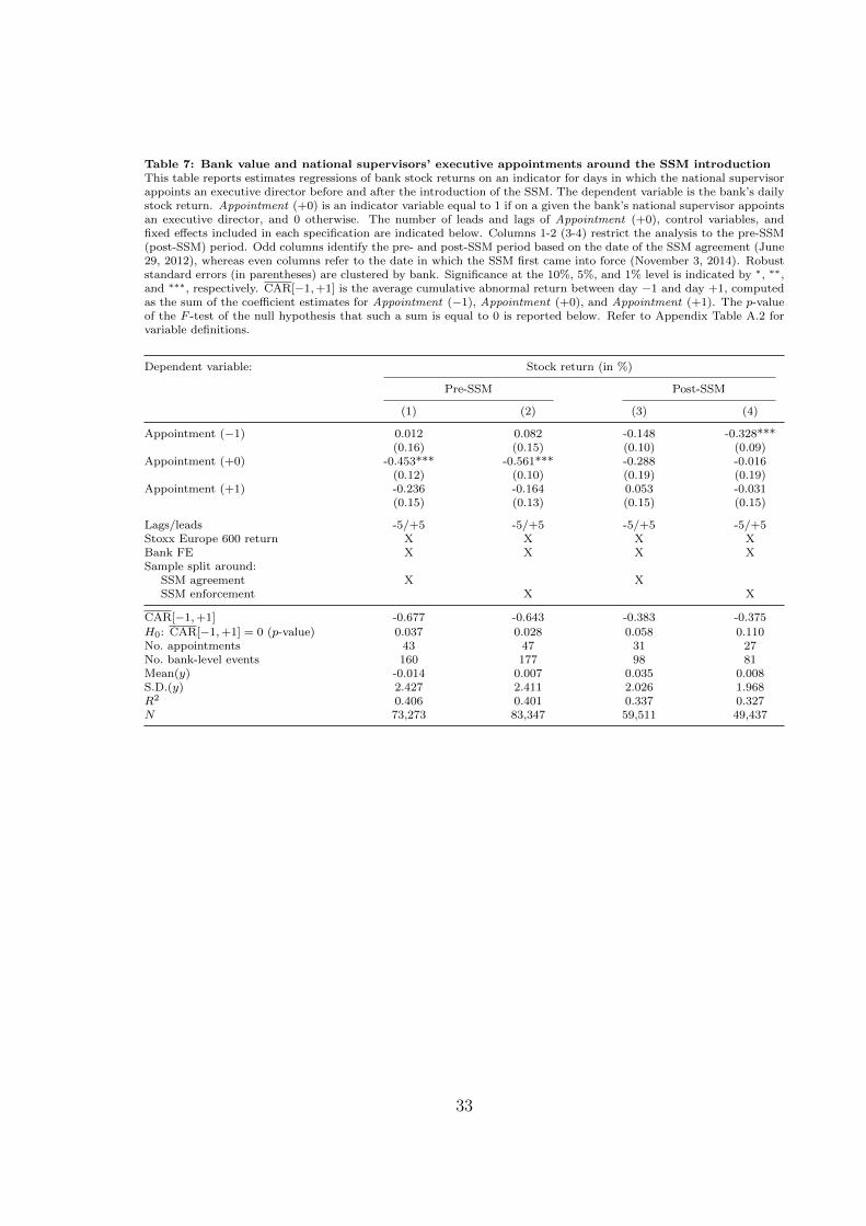
Table 7: Bank value and national supervisors’ executive appointments around the SSM introductionThis table reports estimates regressions of bank stock returns on an indicator for days in which the national supervisorappoints an executive director before and after the introduction of the SSM. The dependent variable is the bank’s dailystock return. Appointment (+0) is an indicator variable equal to 1 if on a given the bank’s national supervisor appointsan executive director, and 0 otherwise. The number of leads and lags of Appointment (+0), control variables, andfixed effects included in each specification are indicated below. Columns 1-2 (3-4) restrict the analysis to the pre-SSM(post-SSM) period. Odd columns identify the pre- and post-SSM period based on the date of the SSM agreement (June29, 2012), whereas even columns refer to the date in which the SSM first came into force (November 3, 2014). Robuststandard errors (in parentheses) are clustered by bank. Significance at the 10%, 5%, and 1% level is indicated by ∗, ∗∗,and ∗∗∗, respectively. CAR[−1,+1] is the average cumulative abnormal return between day −1 and day +1, computedas the sum of the coefficient estimates for Appointment (−1), Appointment (+0), and Appointment (+1). The p-valueof the F -test of the null hypothesis that such a sum is equal to 0 is reported below. Refer to Appendix Table A.2 forvariable definitions.

Dependent variable: Stock return (in %)

Pre-SSM Post-SSM

(1) (2) (3) (4)

Appointment (−1) 0.012 0.082 -0.148 -0.328***(0.16) (0.15) (0.10) (0.09)

Appointment (+0) -0.453*** -0.561*** -0.288 -0.016(0.12) (0.10) (0.19) (0.19)

Appointment (+1) -0.236 -0.164 0.053 -0.031(0.15) (0.13) (0.15) (0.15)

Lags/leads -5/+5 -5/+5 -5/+5 -5/+5Stoxx Europe 600 return X X X XBank FE X X X XSample split around:

SSM agreement X XSSM enforcement X X

CAR[−1,+1] -0.677 -0.643 -0.383 -0.375

H0: CAR[−1,+1] = 0 (p-value) 0.037 0.028 0.058 0.110No. appointments 43 47 31 27No. bank-level events 160 177 98 81Mean(y) -0.014 0.007 0.035 0.008S.D.(y) 2.427 2.411 2.026 1.968R2 0.406 0.401 0.337 0.327N 73,273 83,347 59,511 49,437

33

Table

8:

Bank

valu

eand

SSM

-rela

ted

events

Th

ista

ble

rep

ort

ses

tim

ate

sof

ban

kst

ock

mark

etre

act

ion

toth

em

ost

sali

ent

even

tsth

at

led

toth

ein

trod

uct

ion

of

the

SS

M.

For

each

even

t,aver

age

ab

norm

al

retu

rns

at

days−

1,

0,

an

d+

1(A

R[−

1],

AR

[+0],

an

dA

R[+

1])

aro

un

dth

ean

nou

nce

men

td

ate

,as

wel

las

the

aver

age

cum

ula

tive

ab

norm

al

retu

rnb

etw

een

days−

1,

0,

an

d+

1(C

AR

[−1,+

1])

are

rep

ort

ed.

To

ob

tain

such

esti

mate

s,se

para

teev

ent

stu

die

son

ban

kd

ail

yst

ock

retu

rns

have

bee

nco

nd

uct

edin

the

style

of

the

even

tst

ud

yb

ase

line

spec

ifica

tion

(Colu

mn

4of

Tab

le4).

Inea

chre

gre

ssio

n,

we

lim

itth

esa

mp

leto

the

two

yea

rsaro

un

dth

ere

spec

tive

even

td

ate

.R

ob

ust

stan

dard

erro

rs(i

np

are

nth

eses

)are

clu

ster

edby

ban

k.

Sig

nifi

can

ceat

the

10%

,5%

,an

d1%

level

isin

dic

ate

dby

∗ ,∗∗

,an

d∗∗

∗ ,re

spec

tivel

y.R

efer

toA

pp

end

ixT

able

A.2

for

vari

ab

led

efin

itio

ns.

AR

[−1]

AR

[+0]

AR

[+1]

CA

R[−

1,+

1]

Date

Even

t(1

)(2

)(3

)(4

)

Ju

ne

29,

2012

Eu

rozo

ne

lead

ers

agre

eon

the

esta

bli

shm

ent

of

the

SS

M.

-0.4

08

0.3

20.0

04

-0.0

83

(0.3

41)

(0.6

08)

(0.9

94)

(0.9

24)

Sep

tem

ber

7,

2012

EC

BV

ice

Pre

sid

ent

spee

chat

the

Du

isen

ber

gS

chool

of

Fin

an

ceti

tled

“T

ow

ard

1.4

47***

2.0

34***

1.0

17**

4.4

98***

aE

uro

pea

nB

an

kin

gU

nio

n”

(0.0

00)

(0.0

01)

(0.0

27)

(0.0

00)

Sep

tem

ber

12,

2012

Eu

rop

ean

Com

mis

sion

ad

op

tstw

op

rop

osa

lsfo

rth

ees

tab

lish

men

tof

the

SS

M.

1.3

07***

-0.7

28***

0.1

49

0.7

29

(0.0

02)

(0.0

04)

(0.7

49)

(0.2

00)

Dec

emb

er13,

2012

EC

OF

INre

ach

esa

lan

dm

ark

agre

emen

ton

the

esta

bli

shm

ent

of

the

SS

M.

1.0

48***

0.9

54**

-0.0

45

1.9

57***

(0.0

00)

(0.0

30)

(0.8

52)

(0.0

10)

Dec

emb

er14,

2012

Dis

closu

reof

the

crit

eria

ad

op

ted

by

the

EC

Bto

iden

tify

sign

ifica

nt

ban

ks.

0.9

56**

-0.0

44

0.8

15*

1.7

28**

(0.0

30)

(0.8

58)

(0.0

74)

(0.0

41)

Feb

ruary

12,

2013

EC

BV

ice

Pre

sid

ent

spee

chat

the

Warw

ick

Eco

nom

ics

Su

mm

itti

tled

0.6

02

-1.3

64***

0.1

43

-0.6

19

“F

inan

cial

Sta

bil

ity

Ris

ks,

Mon

etary

Poli

cyan

dth

eN

eed

for

Macr

o-P

rud

enti

al

Poli

cy”.

(0.1

67)

(0.0

02)

(0.7

60)

(0.3

93)

Sep

tem

ber

12,

2013

EU

parl

iam

ent

ap

pro

ves

the

EU

ban

ksu

per

vis

ion

syst

em.

1.2

48***

-0.3

22

-0.7

58**

0.1

68

(0.0

10)

(0.1

31)

(0.0

34)

(0.7

49)

Oct

ob

er23,

2013

EC

Bst

art

sco

mp

reh

ensi

ve

ass

essm

ent

inad

van

ceof

its

sup

ervis

ory

role

.-0

.872**

-1.6

17***

1.0

75***

-1.4

13***

(0.0

35)

(0.0

01)

(0.0

03)

(0.0

06)

Dec

emb

er16,

2013

Dan

iele

Nou

yap

poin

ted

as

Ch

air

of

the

sup

ervis

ory

board

.0.2

79

0.0

19

-0.5

13

-0.2

15

(0.2

93)

(0.9

50)

(0.4

01)

(0.7

22)

Janu

ary

9,

2014

Fou

rd

irec

tors

ap

poin

ted

inth

en

ewD

irec

tora

teG

ener

al

for

sup

ervis

ion

.1.3

46***

0.5

55

-0.7

23**

1.1

79**

(0.0

00)

(0.1

63)

(0.0

17)

(0.0

21)

Janu

ary

22,

2014

Sab

ine

Lau

ten

sch

lager

ap

poin

ted

as

Vic

e-C

hair

of

the

sup

ervis

ory

board

.-0

.133

-0.6

25*

0.7

4-0

.017

(0.6

26)

(0.0

98)

(0.1

05)

(0.9

78)

Feb

ruary

3,

2014

EC

Bm

akes

pro

gre

ssw

ith

the

Ass

etQ

uali

tyR

evie

w(A

QR

)an

dco

nfi

rms

stre

ss-t

est.

0.0

03

-1.2

96***

1.5

2***

0.2

27

para

met

ers

for

com

pre

hen

sive

ass

essm

ent.

(0.9

9)

(0.0

00)

(0.0

00)

(0.6

23)

Marc

h7,

2014

EC

Bap

poin

tsth

ree

rep

rese

nta

tives

toth

eb

an

ksu

per

vis

ory

board

.0.1

36

-0.2

20.6

09*

0.5

25

(0.7

26)

(0.3

45)

(0.0

57)

(0.3

76)

Ap

ril

25,

2014

EC

Bp

ubli

shes

fram

ework

for

SS

Mre

gu

lati

on

.-0

.352

-0.8

92***

-0.3

28*

-1.5

72***

(0.2

99)

(0.0

00)

(0.0

94)

(0.0

01)

Ap

ril

29,

2014

EC

Bsa

ys

that

cap

ital

gap

sfr

om

AQ

Rm

ust

be

cover

edw

ith

CE

T1

inst

rum

ents

.-0

.329*

0.7

93**

-0.6

8**

-0.2

15

(0.0

94)

(0.0

39)

(0.0

22)

(0.6

52)

Ju

ly17,

2014

EC

BV

ice

Pre

sid

ent

says

stri

ctn

ess

of

EC

Bte

stn

ot

just

ab

ou

tre

sult

s.0.9

75***

-0.6

92***

0.0

87

0.3

69

(0.0

07)

(0.0

01)

(0.7

36)

(0.3

92)

Oct

ob

er27,

2014

EC

Bd

iscl

ose

sre

sult

sof

the

AQ

Rex

erci

sean

did

enti

fies

ban

ks

that

nee

dfu

rth

eract

ion

s.1.7

12***

-0.7

66*

-0.1

44

0.8

03

(0.0

00)

(0.0

69)

(0.5

55)

(0.1

13)

Novem

ber

4,

2014

SS

Mst

art

s.-0

.246

0.1

87

-1.7

78***

-1.8

36***

(0.6

54)

(0.6

05)

(0.0

00)

(0.0

28)

34

Table

9:

Bank

debt

valu

eand

nati

onal

sup

ervis

ors’

executi

ve

app

oin

tments

Th

ista

ble

rep

ort

ses

tim

ate

sre

gre

ssio

ns

of

chan

ges

inC

DS

spre

ad

son

an

ind

icato

rfo

rd

ays

inw

hic

hth

en

ati

on

al

sup

ervis

or

ap

poin

tsan

exec

uti

ve

dir

ecto

r.T

he

dep

end

ent

vari

ab

leis

the

ban

k’s

dail

ych

an

ge

insp

read

son

5-y

ear

CD

Sco

ntr

act

sw

ritt

enon

sen

ior

un

secu

red

deb

t.A

ppo

intm

ent

(+0)

isan

ind

icato

rvari

ab

leeq

ual

to1

ifon

agiv

enth

eb

an

k’s

nati

on

al

sup

ervis

or

ap

poin

tsan

exec

uti

ve

dir

ecto

r,an

d0

oth

erw

ise.

Appo

intm

ent,

w/o

fin

.ba

ckgr

ou

nd

(+0)

isan

ind

icato

rvari

ab

leeq

ual

to1

ifon

agiv

end

ay

the

ban

k’s

nati

on

al

sup

ervis

or

ap

poin

tsan

exec

uti

ve

dir

ecto

rw

ith

no

pri

or

fin

an

ceex

per

ien

ce,

an

d0

oth

erw

ise.

Appo

intm

ent,

wit

hfi

n.

back

grou

nd

(+0)

isan

ind

icato

rvari

ab

leeq

ual

to1

ifon

agiv

end

ay

the

ban

k’s

nati

on

al

sup

ervis

or

ap

poin

tsan

exec

uti

ve

dir

ecto

rw

ith

pri

or

fin

an

ceex

per

ien

ce,

an

d0

oth

erw

ise.

Appo

intm

ent,

wit

hli

nk

toba

nk)

(+0

isan

ind

icato

rvari

ab

leeq

ual

to1

ifon

agiv

end

ay

the

ban

k’s

nati

on

al

sup

ervis

or

ap

poin

tsan

exec

uti

ve

dir

ecto

rw

ho

pre

vio

usl

yh

eld

ap

osi

tion

at

the

ban

k,

an

d0

oth

erw

ise.

Th

enu

mb

erof

lead

san

dla

gs

of

the

ap

poin

tmen

tin

dic

ato

rvari

ab

les,

contr

ol

vari

ab

les,

an

dfi

xed

effec

tsin

clu

ded

inea

chsp

ecifi

cati

on

are

ind

icate

db

elow

.R

ob

ust

stan

dard

erro

rs(i

np

are

nth

eses

)are

clu

ster

edby

ban

k.

Sig

nifi

can

ceat

the

10%

,5%

,an

d1%

level

isin

dic

ate

dby

∗ ,∗∗

,an

d∗∗

∗ ,re

spec

tivel

y.C

AR

[−1,+

1]

isth

eaver

age

cum

ula

tive

ab

norm

al

CD

Ssp

read

chan

ge

bet

wee

nd

ay−

1an

dd

ay

+1

aro

un

dth

eev

ent,

com

pu

ted

as

the

sum

of

the

coeffi

cien

tes

tim

ate

sfo

rth

eap

poin

tmen

tin

dic

ato

rvari

ab

leon

days

−1,

+0,

an

d+

1.

Th

ep-v

alu

eof

theF

-tes

tof

the

nu

llhyp

oth

esis

that

such

asu

mis

equ

al

to0

isre

port

edb

elow

.R

efer

toA

pp

end

ixT

ab

leA

.2fo

rvari

ab

led

efin

itio

ns.

Dep

end

ent

vari

ab

le:

∆C

DS

spre

ad

(1)

(2)

(3)

(4)

(5)

(6)

(7)

(8)

Ap

poin

tmen

t(−

1)

0.4

73**

0.4

38*

(2.2

3)

(1.9

6)

Ap

poin

tmen

t(+

0)

0.5

49*

0.5

14*

(1.8

3)

(1.7

0)

Ap

poin

tmen

t(+

1)

0.2

64

0.2

50

(1.0

9)

(0.9

5)

Ap

poin

tmen

t,w

/o

fin

.b

ack

gro

un

d(−

1)

0.6

87

0.7

30*

(1.6

5)

(1.7

3)

Ap

poin

tmen

t,w

/o

fin

.b

ack

gro

un

d(+

0)

0.6

33

0.7

47

(1.1

9)

(1.3

6)

Ap

poin

tmen

t,w

/o

fin

.b

ack

gro

un

d(+

1)

0.3

94*

0.5

09**

(1.8

9)

(2.0

8)

Ap

poin

tmen

t,w

ith

fin

.b

ack

gro

un

d(−

1)

0.2

27

0.1

04

(1.0

6)

(0.5

4)

Ap

poin

tmen

t,w

ith

fin

.b

ack

gro

un

d(+

0)

0.4

48

0.2

43

(1.5

4)

(0.9

0)

Ap

poin

tmen

t,w

ith

fin

.b

ack

gro

un

d(+

1)

0.1

26

-0.0

35

(0.2

6)

(-0.0

6)

Ap

poin

tmen

tof

ad

irec

tor

wit

hli

nk

tob

ank

(−1)

1.3

34***

1.3

89**

(3.0

1)

(2.7

2)

Ap

poin

tmen

tof

ad

irec

tor

wit

hli

nk

tob

ank

(+0)

-0.3

63

-0.2

99

(-0.9

0)

(-0.8

8)

Ap

poin

tmen

tof

ad

irec

tor

wit

hli

nk

tob

ank

(+1)

-0.1

85

-0.0

27

(-0.3

8)

(-0.0

7)

Lags/

lead

s-5

/+

5-5

/+

5-5

/+

5-5

/+

5-5

/+

5-5

/+

5-5

/+

5-5

/+

5S

toxx

Eu

rop

e600

retu

rnX

XX

XX

XX

XS

over

eign

cred

itsp

read

XX

XX

XX

XX

Ban

kF

EX

XX

XX

XX

XM

onth

-yea

rF

EX

XX

X

CA

R[−

1,+

1]

1.2

86

1.2

02

1.7

14

1.9

86

0.8

01

0.3

12

0.7

86

1.0

62

H0:

CA

R[−

1,+

1]=

0(p

-valu

e)0.0

01

0.0

06

0.0

28

0.0

22

0.0

56

0.5

39

0.1

77

0.0

15

No.

ap

poin

tmen

ts69

69

38

38

31

31

10

10

No.

ban

k-l

evel

even

ts167

167

87

87

80

80

12

12

Mea

n(y

)0.0

10

0.0

10

0.0

10

0.0

10

0.0

10

0.0

10

0.0

10

0.0

10

S.D

.(y)

6.9

63

6.9

63

6.9

63

6.9

63

6.9

63

6.9

63

6.9

63

6.9

63

R2

0.0

88

0.1

06

0.0

88

0.1

06

0.0

89

0.1

06

0.0

88

0.1

06

N83,7

24

83,7

24

83,7

24

83,7

24

83,7

24

83,7

24

83,7

24

83,7

24

35

Appendix for“Reverse Revolving Doors in the Supervision of European

Banks”

37

Table A.1: List of national supervisorsThis table lists the national supervisors included in the sample, together with the time span, the number of distinctexecutive directors, and the number of executive-years available for each of them.

Country Institution First year Last year No. executives No. executive-years

AT Osterreichische Nationalbank 2002 2019 13 120AT Financial Market Authority 2002 2019 4 37BE Nationale Bank van Belgie 2002 2019 14 91DE Deutsche Bundesbank 2002 2019 20 135DE Bundesanstalt fur Finanzdienstleistungsaufsicht 2002 2019 14 126ES Banco de Espana 2004 2019 20 182GB Bank of England 2002 2019 16 77GB Prudential Regulation Authority 2012 2019 13 52GB Financial Services Authority 2002 2013 14 57FR Banque de France 2002 2019 9 58IE Central Bank of Ireland 2007 2019 9 44IT Banca d’Italia 2002 2019 15 79NL De Nederlandsche Bank 2002 2019 13 85SE Sveriges Riksbank 2002 2019 16 112

38

Table

A.2

:D

efinit

ion

of

varia

ble

s

Vari

ab

leD

ata

base

sD

efin

itio

n

Ban

kdata

Cost

-to-i

nco

me

rati

oB

an

ksc

op

ean

dO

rbis

Ban

kF

ocu

sN

on

-inte

rest

exp

ense

sover

the

sum

of

net

inte

rest

inco

me

an

doth

erop

erati

ng

inco

me

Imp

air

edlo

an

sover

tota

llo

an

sB

an

ksc

op

ean

dO

rbis

Ban

kF

ocu

sR

ati

oof

imp

air

edlo

an

sover

tota

llo

an

s

Reg

ula

tory

Tie

r1

rati

oB

an

ksc

op

ean

dO

rbis

Ban

kF

ocu

sR

ati

oof

tier

1re

gu

lato

ryca

pit

al

over

risk

wei

ghte

dass

ets

RO

AB

an

ksc

op

ean

dO

rbis

Ban

kF

ocu

sR

etu

rnon

aver

age

ass

ets

Tota

lass

ets

Ban

ksc

op

ean

dO

rbis

Ban

kF

ocu

sB

ook

valu

eof

tota

lass

ets

Eve

nt

stu

dy

data

Ap

poin

tmen

tB

loom

ber

gIn

dic

ato

req

ual

toon

eon

the

day

of

an

an

nou

nce

men

tof

an

ewex

ecu

tive

dir

ecto

rap

poin

tmen

tat

asu

per

-vis

ory

inst

itu

tion

inth

eh

om

eco

untr

yof

the

ban

kA

pp

oin

tmen

t,w

/o

fin

.b

ack

gro

un

dB

loom

ber

gand

manu

-all

yco

llec

ted

Ind

icato

req

ual

toon

eon

the

day

of

an

an

nou

nce

men

tof

an

ewex

ecu

tive

dir

ecto

rap

poin

tmen

tat

asu

per

-vis

ory

inst

itu

tion

inth

eh

om

eco

untr

yof

the

ban

k,

wh

erea

sth

en

ewex

ecu

tive

dir

ecto

rh

as

no

pri

or

fin

an

cein

du

stry

exp

erie

nce

Ap

poin

tmen

t,w

ith

fin

.b

ack

gro

un

dB

loom

ber

gan

dm

anu

-all

yco

llec

ted

Ind

icato

req

ual

toon

eon

the

day

of

an

an

nou

nce

men

tof

an

ewex

ecu

tive

dir

ecto

rap

poin

tmen

tat

asu

per

-vis

ory

inst

itu

tion

inth

eh

om

eco

untr

yof

the

ban

k,

wh

erea

sth

en

ewex

ecu

tive

dir

ecto

rh

as

pri

or

fin

an

cein

du

stry

exp

erie

nce

Ap

poin

tmen

t,w

ith

lin

kto

ban

kB

loom

ber

gan

dm

anu

-all

yco

llec

ted

Ind

icato

req

ual

toon

eon

the

day

of

an

an

nou

nce

men

tof

an

ewex

ecu

tive

dir

ecto

rap

poin

tmen

tat

asu

per

-vis

ory

inst

itu

tion

inth

eh

om

eco

untr

yof

the

ban

k,

wh

erea

sth

en

ewex

ecu

tive

dir

ecto

rh

as

ali

nk

thro

ugh

her

CV

toa

the

ban

kin

the

sam

eco

untr

yC

DS

spre

ad

Blo

om

ber

gan

dD

ata

s-tr

eam

Ban

kC

DS

spre

ad

Sto

xx

Eu

rop

e600

retu

rnB

loom

ber

gR

etu

rnof

Sto

xx

Eu

rop

e600

stock

mark

etin

dex

Rec

essi

on

Ow

nca

lcu

lati

on

sIn

dic

ato

req

ual

toon

eif

an

econ

om

yex

per

ien

ced

two

qu

art

ers

of

neg

ati

ve

gro

wth

inG

DP

Sover

eign

cred

itsp

read

Blo

om

ber

gD

iffer

ence

bet

wee

nso

ver

eign

yie

ldan

dre

fere

nce

rate

Sto

ckre

turn

Blo

om

ber

gS

tock

retu

rnS

tock

retu

rns

vola

tili

tyB

loom

ber

gS

tan

dard

dev

iati

on

of

stock

retu

rns

39

Table A.3: Bank value and national supervisors’ executive appointments (in event time)This table reports estimates event-time regressions of bank stock returns on an indicator for days in which the nationalsupervisor appoints an executive director. The dependent variable is the bank’s daily stock return. Appointment (+0)is an indicator variable equal to 1 if on a given the bank’s national supervisor appoints an executive director, and 0otherwise. Appointment, w/o fin. background (+0) is an indicator variable equal to 1 if on a given day the bank’snational supervisor appoints an executive director with no prior finance experience, and 0 otherwise. Appointment,with fin. background (+0) is an indicator variable equal to 1 if on a given day the bank’s national supervisor appoints anexecutive director with prior finance experience, and 0 otherwise. Appointment, with link to bank) (+0 is an indicatorvariable equal to 1 if on a given day the bank’s national supervisor appoints an executive director who previously helda position at the bank, and 0 otherwise. The number of leads and lags of the appointment indicator variables, controlvariables, and fixed effects included in each specification are indicated below. The estimation sample is restricted tothe window of [−50,+50] days around each appointment event, and excludes events exhibiting overlapping windows.Robust standard errors (in parentheses) are clustered by bank. Significance at the 10%, 5%, and 1% level is indicatedby ∗, ∗∗, and ∗∗∗, respectively. CAR[−1,+1] is the average cumulative abnormal stock return of the null hypothesisthat such a sum is equal to 0 is reported below. Refer to Appendix Table A.2 for variable definitions.

Dependent variable: Stock return (in %)

(1) (2) (3) (4)

Appointment (+0) -0.306***(-3.55)

Appointment, w/o fin. background (+0) -0.660***(-4.79)

Appointment, with fin. background (+0) 0.024(0.23)

Appointment of a director with link to bank (+0) 0.511**(2.49)

Lags/leads -10/+10 -10/+10 -10/+10 -10/+10Stoxx Europe 600 return X X X XBank FE X X X X

CAR[−1,+1] -0.329 -0.613 -0.126 0.743

H0: CAR[−1,+1] = 0 (p-value) 0.182 0.058 0.837 0.897No. appointments 67 38 33 14No. bank-level events 263 146 140 16Mean(y) -0.003 -0.026 0.029 -0.035S.D.(y) 2.279 2.352 2.354 2.405R2 0.363 0.344 0.402 0.545N 23,536 13,378 13,495 1,556

40

Table A.4: Bank value, national supervisors’ executive appointments, and their background (jointestimation)This table reports estimates regressions of bank stock returns on indicators for days in which the national supervisorappoints an executive director with a certain work experience. The dependent variable is the bank’s daily stock return.Appointment, with fin. background (+0) is an indicator variable equal to 1 if on a given day the bank’s nationalsupervisor appoints an executive director with prior finance experience, and 0 otherwise. Any other appointment (+0)is an indicator variable equal to 1 if on a given day the bank’s national supervisor appoints an executive directorand Appointment, with fin. background (+0)= 0, and 0 otherwise. The number of leads and lags of the appointmentindicator variables, control variables, and fixed effects included in each specification are indicated below. Robuststandard errors (in parentheses) are clustered by bank. Significance at the 10%, 5%, and 1% level is indicated by ∗,∗∗, and ∗∗∗, respectively. ∆CAR[−1,+1] is the difference between finance-related and other appointments in terms ofaverage cumulative abnormal return between day −1 and day +1 around the event. The p-value of the F -test of the nullhypothesis that such a difference is equal to 0 is reported below. Refer to Appendix Table A.2 for variable definitions.

Dependent variable: Stock return (in %)

(1) (2)

Appointment, with fin. background (−1) -0.190 -0.148(0.12) (0.12)

Appointment, with fin. background (+0) -0.118 -0.059(0.11) (0.11)

Appointment, with fin. background (+1) 0.032 0.084(0.09) (0.09)

Any other appointment (−1) 0.091 0.057(0.15) (0.16)

Any other appointment (+0) -0.634*** -0.669***(0.15) (0.16)

Any other appointment (+1) -0.262* -0.296*(0.16) (0.15)

Lags/leads -5/+5 -5/+5Stoxx Europe 600 return X XBank FE X XMonth-year FE X

∆CAR[−1,+1] 0.529 0.785

H0: ∆CAR[−1,+1] = 0 (p-value) 0.073 0.012No. appointments 74 74No. bank-level events 258 258Mean(y) 0.008 0.008S.D.(y) 2.256 2.256R2 0.380 0.386N 132,784 132,784

41