Working Paper No. 644

How Rich Countries Became Rich and Why Poor Countries Remain

Poor: It’s the Economic Structure . . . Duh!*

by

Jesus Felipe Utsav Kumar

Arnelyn Abdon Asian Development Bank, Manila, Philippines

December 2010

* This paper represents the views of the authors and not those of the Asian Development Bank, its executive directors, or the member countries that they represent. Participants in lectures given by Jesus Felipe at Singapore’s Civil Service College and at the Singapore Economic Policy Forum in October 2010 made very useful comments and suggestions. Nevertheless, the usual disclaimer applies. Contacts: jfelipe@adb.org (corresponding author); ukumar.consultant@adb.org; aabdon.consultant@adb.org

The Levy Economics Institute Working Paper Collection presents research in progress by Levy Institute scholars and conference participants. The purpose of the series is to disseminate ideas to and elicit comments from academics and professionals.

Levy Economics Institute of Bard College, founded in 1986, is a nonprofit, nonpartisan, independently funded research organization devoted to public service. Through scholarship and economic research it generates viable, effective public policy responses to important economic problems that profoundly affect the quality of life in the United States and abroad.

Levy Economics Institute

P.O. Box 5000 Annandale-on-Hudson, NY 12504-5000

http://www.levyinstitute.org

Copyright © Levy Economics Institute 2010 All rights reserved

2

ABSTRACT

Becoming a rich country requires the ability to produce and export commodities that

embody certain characteristics. We classify 779 exported commodities according to two

dimensions: (1) sophistication (measured by the income content of the products

exported); and (2) connectivity to other products (a well-connected export basket is one

that allows an easy jump to other potential exports). We identify 352 “good” products

and 427 “bad” products. Based on this, we categorize 154 countries into four groups

according to these two characteristics. There are 34 countries whose export basket

contains a significant share of good products. We find 28 countries in a “middle product”

trap. These are countries whose export baskets contain a significant share of products that

are in the middle of the sophistication and connectivity spectra. We also find 17 countries

that are in a “middle-low” product trap, and 75 countries that are in a difficult and

precarious “low product” trap. These are countries whose export baskets contain a

significant share of unsophisticated products that are poorly connected to other products.

To escape this situation, these countries need to implement policies that would help them

accumulate the capabilities needed to manufacture and export more sophisticated and

better connected products.

Keywords: Bad Product; Capabilities; “Low Product” Trap; “Middle Product” Trap;

Proximity; Sophistication; Structural Transformation

JEL Classifications: O14, O25, O57

1

1. INTRODUCTION

The study of the reasons why some countries achieve sustained growth that allows them

to develop while many others cannot do it and seem not to be able to progress has been at

the core of economics since the days of the founding fathers of the discipline (i.e., Smith,

Ricardo, Malthus, and their critic, Marx), whose concern was the study of the

determinants of the wealth of nations. Later on, after WWII, with the birth of

development economics as a field, this has been, and continues to be, the central question

of the discipline. In the words of Lucas (1988): “The consequences for human welfare

involved in questions like these are simply staggering: Once one starts to think about

them, it is hard to think about anything else” (Lucas 1988: 5).1

Explaining why most countries in the world are in some sort of economic trap is

not easy. Standard growth models like the Harrod (1939), Domar (1946), Solow (1956),

or the myriad of endogenous growth models developed since the 1980s (see Barro and

Sala-i-Martin [1995] or Aghion and Howitt [1998] for expositions) somehow address the

question of why some countries achieve sustained growth while some others cannot do it,

but they were not conceived with the objective of explaining differences between

developed and developing countries, and much less explaining why so many countries in

the world are trapped.

Arthur Lewis (1955: 208) argued that the central fact of economic development is

rapid capital accumulation. Development requires increasing the annual rate of net

investment from 5 percent or less to 12 percent or more. “This is what we mean by an

Industrial Revolution.” The evidence of the last fifty five years seems to indicate that

while investment does matter for growth and development, developing takes much more

than increasing the rate of investment to at least 12 percent.

The reality is that the world has been divided for quite some time among three

groups: (i) the club of rich nations, with income per capita above $12,000, according to

1 The questions Lucas refers to are in the previous sentence of his paper: “Is there some action a Government of India could take that would lead the Indian economy to grow like Indonesia’s or Egypt’s? If so, what exactly? If not, what is it about the ‘nature of India’ that makes it so?” (Lucas 1988: 5).

2

the World Bank, using 2007 data; (ii) a very large group of poor countries with income

per capita below $1,000; and (iii) a group of countries that falls in between these two.

These countries seem to move forward, but slowly, with the consequence that very few

graduate and make it to the club of rich countries. Some of these nations are Brazil,

Mexico, Argentina, Malaysia, or Thailand. They are referred to as being in a “middle

income trap.” However, most countries in the world have not even reached this stage. Is it

because the rate of investment is below 12 percent? No, today we know that their

problem is much more complex. 2

In this paper, we attempt to provide empirical content to the traps that many

countries face in order to develop. To this purpose, we study the characteristics of their

export basket. We classify 154 countries according to two dimensions of an export basket

comprising 779 products: (i) sophistication (measured by the income content); and (ii)

connectivity to other products (a well-connected export basket is one that allows an easy

jump to other potential exports). There are only 34 countries in the world that export

mostly sophisticated and well-connected products. We identify 28 countries in the world

that are in a “middle product trap,” 17 countries that are in a “middle-low” product trap,

and 75 countries that are in a difficult and precarious “low product trap.” To solve this

fundamental development problem requires, first, an understanding of the relationship

between poverty and the structure of production, i.e., what countries produce and export

determines who they are in the world; and second, implementation of appropriate and

realistic economic policies. Specifically, we argue that what allows countries to become

rich has to do with the type of economic activities they engage in (i.e., the type of goods

they end up producing and exporting), and with the policies that they implement to

promote and develop certain types of industries. 2 The role of investment in development is neither well understood nor even agreed upon by economists. While the proposition that investment is key for growth seems obvious, the empirical evidence is not conclusive. For example, Easterly (2002: 39–42) and Oulton and O’Mahony (1994) claim that capital does not play any special role; while Prichett (2003: 217–21) claims that “except for the causality issue, the role of physical investment in growth is well understood.” On the issue of causality, Blomstrom, Lipsey, and Zejan (1996) used causality tests and found that a faster rate of GDP growth causes a higher investment-output ratio and not vice versa. If this is true, the implication is that investment is not a key determining exogenous variable in the growth process. Once growth is underway, the resulting profits will cause the investment rate to increase in a Keynesian fashion. As Kaldor (1970) pointed out, Henry Ford did not build up his automobile business from high initial savings, but from the profits his factory generated.

3

There are three strands of the development literature that are extremely relevant if

one wants to explain why some countries make it while many others do not. They run

parallel and complement each other. First, there are models that specifically deal with the

question of why some countries get into “traps” that do not allow them to maintain

sustained growth. Perhaps the oldest trap model, at least formalized in mathematical

terms, is Nelson’s (1956) low-level poverty trap, which intends to integrate population

and development theory by recognizing the interdependence between population growth,

per capita income, and national income growth.3 This model demonstrates the difficulties

that developing countries face in achieving a self-sustained rise in living standards. The

low-level equilibrium trap refers to a situation where per capita income is permanently

depressed as a consequence of a fast population growth, faster than the growth in national

income. In dynamic terms, as long as this happens, per capita income is forced down to

the subsistence level. Myrdal’s (1957) model of “cumulative causation” is also part of the

same tradition. Myrdal argued that economic and social forces produce tendencies toward

disequilibrium, which tends to persist and even widen over time. Myrdal argued, for

example, that following an exogenous shock that generates disequilibrium between two

regions, a multiplier-accelerator mechanism produces increasing returns in the favored

region such that the initial difference, instead of closing as a result of factor mobility,

remains and even increases.4

Second, since the early days of development economics, it was recognized that

development is about the transformation of the productive structure and the accumulation

of the capabilities necessary to undertake this process. The structural transformation

3 The idea of traps was also present in the writings of the classical authors, who argued that, in the long run, the supply curve of labor was horizontal at the subsistence wage, i.e., the level of the real wage at which birth and death rates equalize. This rate is just high enough to reproduce the population and labor force without change. Malthus assumed that the labor supply would be closely related to population, so that a constant population would also mean a constant labor supply. In this model, if the wage rate were to rise above subsistence, the population would grow, and the increased supply of labor would tend to force the wage downward. If the wage rate were to fall below subsistence, high infant mortality would lead the population to shrink, and the resulting decline in the supply of labor would tend to force the wage upward. Over a period of time long enough to allow for these changes in population, the wage in this model will tend to remain close to the subsistence level. 4 Myrdal also argued that, through trade, the developing countries have been forced into the production of goods with inelastic demand with respect to both price and income.

4

literature argues that economic development is a process in which new activities emerge,

old ones disappear, and the weight of all economic activities and their patterns of

interaction change. This is closely related to the notion of structural change—the growing

importance of non-agricultural sectors in production and employment. This is the

tradition of Kuznets (1966), Kaldor (1967), or Chenery, Robinson, and Syrquin (1986),

among others. Specifically, structural change shows up in changes in the shares of labor

of the different sectors, typically with a decline in that of agriculture and an increase in

those of the nonagricultural sectors. For many years, development was equated with

industrialization. The importance of manufacturing derives from its potential for strong

productivity growth and the high income elasticity of demand for manufactures. As labor

and capital move into these activities, average productivity in the economy increases.

Today, it is believed that some services, based on new technologies and standardization

of delivery, enable substantial productivity gains in some activities (Felipe et al. 2009).

Examples of these sectors are transport services, financial operations, wholesale trade,

and renting services.

The countries that have succeeded in this process are those that have managed to

change the productive structure of the economy, and have been able to produce and

export a more diversified and sophisticated product basket. This is the recent experience

of some countries in Asia, e.g., Korea and Singapore. China is undergoing a deep process

of structural transformation that, to a large extent, explains its rapid growth. On the other

hand, the countries that have failed are those that are not able to engineer this process.

They get stuck in the production and export of a relatively narrow range of goods that are

often unsophisticated.

The recent work of Hidalgo et al. (2007) is a novel contribution to the structural

transformation literature. These authors introduce the product space, an application of

network theory that yields a graphical representation of all products exported in the

world. Products are linked through lines that represent their proximity, defined as the

conditional probability of exporting one product given that they also export the other one.

Using the product space, Hausmann and Klinger (2007) argue that countries

change their export mix by jumping to products that are nearby, in the sense that these

5

other products use similar capabilities to those used by the products in which they excel

(i.e., those products in which they have revealed comparative advantage [RCA]).

According to this capabilities approach, comparative advantage depends more on the

nation’s ability (i.e., capability) to understand, master, and use technologies than on

factor endowments (see also Lall 1992, 2000a, and 2000b).

Third is the literature on capabilities à la Sutton (2001, 2005). Becoming a rich

country is about being able to earn higher real wages. In the same vein as Hidalgo et al.

(2007), Sutton argues that some economic activities are more lucrative than others.

Countries that specialize in such activities enjoy a higher level of real wages. But unlike

the traditional neoclassical model, where higher real wages are the result of an increasing

capital-labor ratio, Sutton argues that the primary driver of growth is the gradual build-up

of firms’ capabilities.

The rest of the paper is organized as follows. Section 2 discusses the concept of

capabilities in the context of the product space and a country’s growth prospects. Section

3 discusses the methodology and the various concepts used to classify products as well as

countries. We define and identify “bad” products. These are products that have low

sophistication and/or are not well-connected to other products. Based on this, we identify

countries that are in the “low” and “middle” product traps. Our results indicate that many

countries in the world (in fact, most of them) export bad products, i.e., the largest number

of commodities exported with RCA fall into these groups. On the other hand, there are

other countries that export some of all kinds of products, i.e., both “good” and “bad”

products. Having capabilities to excel in products that are not bad gives these countries

an opportunity to switch to other more sophisticated and better connected products.

Specifically, we identify three groups of countries (comprising a total of 120 countries)

that fall into the “low” or “middle product” trap, plus one group of 34 countries that

produce “good” products, i.e., sophisticated and well-connected. Section 4 provides some

policy recommendations for the various groups of countries identified. Section 5

concludes.

6

2. PRODUCT TRAPS AND DEVELOPMENT

A key challenge that most countries in the world face is how to upgrade and diversify

their export basket. Many countries have been able to exploit their low-wage advantage

to attract foreign direct investment into many industries. However, the challenges to

deepen industrial capabilities, upgrade the skills of the local labor force, set up and build

innovation, research, and development capacity in the domestic economy, and move to

high-value added and more sophisticated products are significant.5 Why upgrade and

diversify? In recent research, Hidalgo et al. (2007) and Hausmann, Hwang, and Rodrik

(2007) recognize the central role that structural transformation plays in development.

Specifically, they argue that while growth and development are the result of structural

transformation, not all activities have the same consequences for a country’s growth

prospects. The implication is that a sustainable growth trajectory must involve the

introduction of new goods and not merely involve continual learning on a fixed set of

goods. Hausmann, Hwang, and Rodrik (2007) show that, after controlling for other

factors such as initial per capita income, countries with a more sophisticated export

basket grow faster. In other words, what a country exports does matter for subsequent

growth. De Ferranti et al. (2000) show that export diversification is associated with a

higher GDP growth.

Standard trade theory postulates that the main determinant of a country’s

comparative advantage, and therefore its trade pattern, is the relative factor endowment.

Changes in a country’s export basket are a result of the changing comparative advantage

based on factor accumulation. The idea is to get the prices right for the various factors of

production so that firms select the appropriate techniques of production. Factor

accumulation leads to factor price changes, which induce changes in the technique of

production. Countries grow by way of accumulating physical or human capital or by

improving the way various factors of production are mixed (total factor productivity).

5 See, for example, Malaysia’s New Economic Model (National Economic Advisory Council: http://www.neac.gov.my/content/download-option-new-economic-model-malaysia-2010), which stresses the need to upgrade from assembly to product development. Most developing countries have similar plans.

7

This brings about a change in the composition of the export basket. Thus, structural

transformation is the result of changes in underlying fundamentals such as education,

financial resources, and overall productivity.

However, export diversification and upgrading are not easy. This is because

venturing into a new activity entails a significant amount of uncertainty about the

profitability of the new venture. The first entrant into this new activity has to engage in

some sort of “cost discovery” (Hausmann and Rodrik 2003). The new activity may have

high social returns but the costs are all private. This is because if the venture fails, all the

costs are borne by the entrant. However, if the venture succeeds, others on the margin

will be quick to enter the activity.

Another possible reason why export diversification is not easy is that many new

activities may require other large-scale investments that are critical to the profitability of

the new activity itself. For example, agroprocessing industries may require well-

developed cold storage transportation systems, logistics and transport networks, well-

established regulatory bodies to provide phytosanitary clearances and permits, and

marketing of a country abroad as a reputable source of agro-based products. All these

complementary activities involving high fixed costs are unlikely to be provided by the

private sector, or are unlikely to be developed by the firms themselves, given the public-

good nature of many such services. As a result, the new activity may not find any takers.

In other words, there is a coordination failure. As a result, the new activity may fail to

develop.

Export diversification and upgrading involves venturing into new activities, which

may involve information and coordination externalities. In some activities and in some

countries there may be a long learning phase with a considerable amount of risk and

uncertainty. In other activities and countries the learning phase might be shorter. The

extent of policy response will therefore vary.

Hausmann and Klinger (2007) investigate the process by which countries are able

to diversify their export mix. They argue that countries change their export mix by

moving to products “nearby” to the products in which they already excel (i.e., those

products that they export with RCA). This is based on the idea that each product requires

8

a specific set of capabilities, and if a country has RCA in that product, then that country

has accumulated the product-specific capabilities. What are these capabilities? They are:

(i) human and physical capital, the legal system, institutions, etc. that are needed to

produce a product (hence, they are product-specific, not just a set of amorphous factor

inputs); (ii) at the firm level, they are the “know-how” and working practices held

collectively by the group of individuals comprising the firm; and (iii) the organizational

abilities that provide the capacity to form, manage, and operate activities that involve

large numbers of people. According to Sutton (2001, 2005), capabilities manifest

themselves as a quality-productivity combination. A given capability is embodied in the

tacit knowledge of the individuals who comprise the firm’s workforce. The quality-

productivity combinations are not a continuum from zero; rather, there is a window with

a “minimum threshold” below which the firm would be excluded from the market.

Therefore, capabilities are largely nontradable inputs.

A country’s ability to foray into new products depends on whether the set of

existing capabilities can be easily redeployed for the production and export of new

products. This idea implies that it is probably easier for a country that exports T-shirts,

for example, to add shorts rather than smart phones to its export basket. On the other

hand, it is very likely that a country that exports basic cell phones has the capabilities to

add smart phones to its export basket. The implication is that it is easier to start producing

a “nearby” product (in terms of required capabilities to export it successfully) than a

product that is “far away” and requires capabilities that the country probably does not

possess.

Hidalgo et al. (2007) conceptualize these ideas in the newly developed product

space. The rationale behind the product space is that if two goods need similar

capabilities, a country should show a high probability of exporting both with comparative

advantage. Thus, the barriers preventing entry into new products are less binding for

products that use similar capabilities.

The product space is highly heterogeneous. Some products are close-by to others

(because they require similar capabilities), while some others are in a sparse area of the

product space. In the first case, it easy to jump from one product into another one (and

9

therefore export the new one with comparative advantage), while in the second case, it is

difficult. The core of the product space, the area with many products close by, comprises

chemicals, machinery, and metal products. The periphery consists of petroleum, raw

materials, tropical agriculture, animal products, cereals, labor-intensive goods, and

capital-intensive goods (excluding metal products). Core products also tend to be more

sophisticated than those in the periphery.

The heterogeneous structure of the product space has important implications for

structural change. If a country exports goods located in a dense part of the product space,

then expanding to other products is much easier because the set of already acquired

capabilities can be easily redeployed for the production of other nearby products. This is

likely to be the case of different types of machinery or of electronic goods. However, if a

country specializes in the peripheral products, this redeployment is more challenging as

no other set of products requires similar capabilities. This is the case of natural resources

such as oil.

A country’s position within the product space, therefore, signals its capacity to

expand to more sophisticated products, thereby laying the groundwork for future growth.

Countries that export products that have few linkages with other products (i.e., countries

that have accumulated capabilities that are hard to redeploy) or countries that have not

accumulated sufficient capabilities to jump to other products cannot generate sustained

long-term growth.

We use a country’s position in the product space to classify it according to two

product characteristics, sophistication (PRODY) and connectivity to other products

(PATH). This, in turn, informs us on the extent of policy interventions that might be

required to get these countries out of “unsophisticated” and “unconnected” products so

that they can undertake structural transformation.

10

3. METHODOLOGY

As argued above, accumulated capabilities are critical for a country’s development

prospects. Under the capabilities approach, the shift of a country’s output and

employment structure away from low value-added activities into high value-added

activities might not be an easy task because venturing into new activities is dependent on

the capabilities already accumulated, i.e., the process is path dependent. This is not to say

that output and employment structures are rigid and cannot be changed. What it means is

that the accumulation of new capabilities, and therefore the ability to venture into new

products, is the result of a long and a cumulative process, one that involves a mix of

learning, building institutional capacity, and an appropriate business environment (Lall

2000a; Hausmann and Klinger 2006; Hausmann, Hwang, and Rodrik 2007; Hidalgo et al.

2007). Accumulating and developing capabilities may require specific and targeted

government policy interventions.

Using a twofold criteria, we classify countries and examine the kind and the

degree of policy interventions that they would need to implement in order to accumulate

the capabilities that would allow them to bring about a significant change in their output

and employment structure, i.e., induce faster structural process. Our discussion in the

previous section has highlighted the role of the kind of products that a country exports

with RCA. To this end, we classify products based on two characteristics: (i) product

sophistication and (ii) path.

3.1 Product Classification

Following Hausmann, Hwang, and Rodrik (2007), we calculate the sophistication level of

a product as the weighted average of the GDP per capita of the countries exporting that

product.6 Algebraically:

6 Lall, Weiss, and Zhang (2006) also develop a similar measure of product sophistication. Their measure is a weighted average of the mean income of ten groups of countries (countries are divided into ten groups according to income) and the weights are the share of the ten groups in the world exports of a product. While not exactly the same as that of Hausmann, Hwang, and Rodrik (2007), the two measures rely on income of countries exporting a product to capture product sophistication.

11

ci

cii

i cc

ci

cici

xvalxval

PRODY GDPpcxval

xval

⎡ ⎤⎢ ⎥⎢ ⎥⎢ ⎥= ×⎢ ⎥⎛ ⎞⎢ ⎥⎜ ⎟⎢ ⎥⎜ ⎟⎢ ⎥⎝ ⎠⎣ ⎦

∑∑

∑ ∑

(1)

where xvalci is the value of country c’s export of commodity i and GDPpcc is country c’s

per capita GDP. We calculate PRODY for 779 products using highly disaggregated trade

data (SITC-Rev.2 4-digit level, UNCOMTRADE Database) for 2003–07, and use the

average of the five years. GDP per capita (measured in 2005 PPP$) is from the World

Development Indicators. PRODY is measured in 2005 PPP$. It varies from a low of

$1,182 for “fabrics, woven of jute or other textile bast fibers of heading 2640” to a high

of $35,885 for “halogenated derivatives of hydrocarbons.”

The rationale that underlies PRODY is that, absent any trade interventions, high-

income countries are able to export despite higher wages because of the characteristics of

the products. One such characteristic is the level of technology embedded in their

products. However, this is not the only reason. Other reasons why activities are located in

high per capita income countries include the availability of natural resources, the quality

of infrastructure, intellectual property rights, the degree of divisibility of the production

process, transportation costs, and possibilities of knowledge spillovers from

agglomeration, especially in the case of research- and development-intensive activities.7

Thus, PRODY, not only reflects technological sophistication, but also incorporates these

other factors.

7 The location of activities, especially in recent times with the advancements in supply-chain management, logistics, and information technology, could also be a reflection of the extent to which production processes can be fragmented and located in different places to take advantage of low labor costs. Lall, Albaladejo, and Zhang (2004) note that industries with discrete production processes see greater fragmentation compared to those with continuous production processes. They further note that within the former, products with high value-to-weight ratios and some processes with high labor intensity and relatively simple skill needs are easier to fragment. Thus, production processes in some industries such as electronics are highly divisible, less so in the case of automotive industry, and least in the case of aerospace industry.

12

The second criterion segregates products according to how easily the capabilities

that they embody can be redeployed and used to export other products. Recall that we

have argued that development is a path-dependent process, and whether or not a country

is able to venture into new activities is determined by the existing set of capabilities. In

simple terms, we want to know whether the capabilities that allow a country to export

basic mobile phones, for example, can be redeployed to export another product, for

example smart phones or luxury cars.

Hidalgo et al. (2007) introduce the notion of “proximity.” It is a measure of

whether a country that exports a product will be able to export another one. Proximity

between two products i and j, denoted ijϕ , is the minimum of the pairwise conditional

probabilities that a country exports a good given that it exports another one.

Algebraically:

( ) ( ){ }ij i j j iP RCA RCA P RCA RCAmin | , |ϕ = , 0≤φij≤1 (2)

where, ( )i jP RCA RCA| is the conditional probability that a country exports good i with

RCA (RCAi) given that it already exports good j also with RCA (RCAj).8 Since the

measure of proximity involves using the minimum of the pairwise conditional

probabilities, the matrix of conditional probabilities is symmetric.

We use Balassa’s (1965) measure of RCA. It is the ratio of the export share of a

product in the country’s export basket to the same share at a worldwide level.

Algebraically:

8 The conditional probability that a country exports good i with RCA given that it exports good j also with RCA is calculated as the ratio of the number of countries that export both goods i and j with RCA to the number of countries that export good j with RCA. Then we choose the smaller of the two conditional probabilities, which implies (given that they only differ in the denominator) that we choose the one whose denominator is larger, i.e., the more ubiquitous product. Given that we have 779 products, we calculate a total of (779×778)/2=303,031 proximities.

13

∑∑∑

∑=

i cci

cci

ici

ci

ci

xval

xval

xvalxval

RCA (3)

where xvalci is the value of country c’s export of commodity i. 9 For purposes of our

analysis, country c exports product i with RCA if RCAci>1.

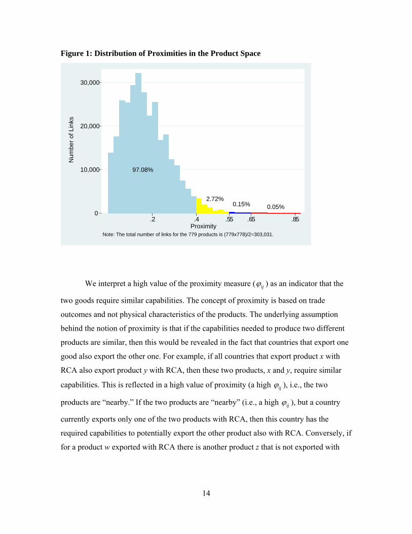
Figure 1 shows the distribution of proximities in the product space. The figure

reveals that this distribution is highly skewed, as most linkages (proximities) are very

weak, below 0.4. Table 1 shows the average proximity within and among 11 product

groups classified according to Leamer’s (1984) classification.10 “Within” proximities

measure the easiness of jumping across products in a given group. On the other hand,

“among” proximities measure the easiness of jumping from one group to the other one.11

The former are significantly higher, reflecting the fact that moving within a group is, in

general, easier than moving out.

9 One word of caution: the index of RCA can be problematic, especially if used for comparison of different products. For example, a country very well endowed with a specific natural resource can have an RCA in the thousands. However, the highest RCA in automobiles is about 3.6. 10 Appendix table 1 shows Leamer’s (1984) classification. Note that the original Leamer classification divides products into ten groups and does not classify some of the SITC (Rev. 2) 2-digit categories. These are categorized as in Hidalgo et al. (2007). Also, the Leamer (1984) category “capital-intensive products” is split into two: capital-intensive products (excluding metals) and metal products. 11 Both within and between proximities are unweighted averages and, as discussed above, they are the average of the minimum of the two possible conditional probabilities.

14

Figure 1: Distribution of Proximities in the Product Space

0

10,000

20,000

30,000

Num

ber o

f Lin

ks

.2 .4 .55 .65 .85Proximity

Note: The total number of links for the 779 products is (779x778)/2=303,031.

97.08%

2.72%0.15% 0.05%

We interpret a high value of the proximity measure ( ijϕ ) as an indicator that the

two goods require similar capabilities. The concept of proximity is based on trade

outcomes and not physical characteristics of the products. The underlying assumption

behind the notion of proximity is that if the capabilities needed to produce two different

products are similar, then this would be revealed in the fact that countries that export one

good also export the other one. For example, if all countries that export product x with

RCA also export product y with RCA, then these two products, x and y, require similar

capabilities. This is reflected in a high value of proximity (a high ijϕ ), i.e., the two

products are “nearby.” If the two products are “nearby” (i.e., a high ijϕ ), but a country

currently exports only one of the two products with RCA, then this country has the

required capabilities to potentially export the other product also with RCA. Conversely, if

for a product w exported with RCA there is another product z that is not exported with

15

RCA by any country, then exporting these two products must involve different

capabilities; this will be represented by a low proximity ( ijϕ ).

Table 1: Average Proximity within and between Leamer Groups PET RAW FOR TRO ANI CER LAB CAP MET MAC CHE

PET 0.356

RAW 0.111 0.335

FOR 0.106 0.157 0.513

TRO 0.126 0.147 0.174 0.454

ANI 0.119 0.146 0.183 0.198 0.435

CER 0.105 0.127 0.141 0.163 0.160 0.286

LAB 0.105 0.131 0.178 0.167 0.158 0.131 0.434

CAP 0.116 0.133 0.171 0.169 0.160 0.144 0.212 0.480

MET 0.135 0.170 0.221 0.175 0.169 0.149 0.204 0.223 0.568

MAC 0.109 0.113 0.158 0.110 0.121 0.108 0.168 0.169 0.205 0.447

CHE 0.145 0.140 0.162 0.147 0.160 0.141 0.157 0.166 0.204 0.198 0.485 Note: PET-Petroleum; RAW-Raw materials; FOR-Forest products;

TRO-Troical agriculture; ANI-Animal products; CER-Cereals; LAB-Labor-intensive; CAP-Capital-intensive (exc. Metals); MET-Metals; MAC-Machiner; CHE-Chemicals.

For each product, we measure the proximity of that product to all other products. This

measure is called PATH (Hausmann and Klinger 2006) and is simply the sum of all

proximities of product i to each of the other products. Algebraically:

i i jj

PATH ϕ=∑ , 0≤ PATHi≤ 778 (No. of products -1) (4)

Products with a high PATH are those that use capabilities that are similar to those used

by many other products.

To calculate the proximities, we first calculate the RCA index for a country’s

exports of commodity i using equation (3) for each of the five years from 2003 to 2007.

We then average the five values. If the averaged RCA is greater than one, then the

country has RCA in commodity i. We then obtain the proximities (as in equation (2)) of

16

each product with respect to all the other 778 products. Finally, proximities are used to

obtain the PATH of each product (equation (4)).

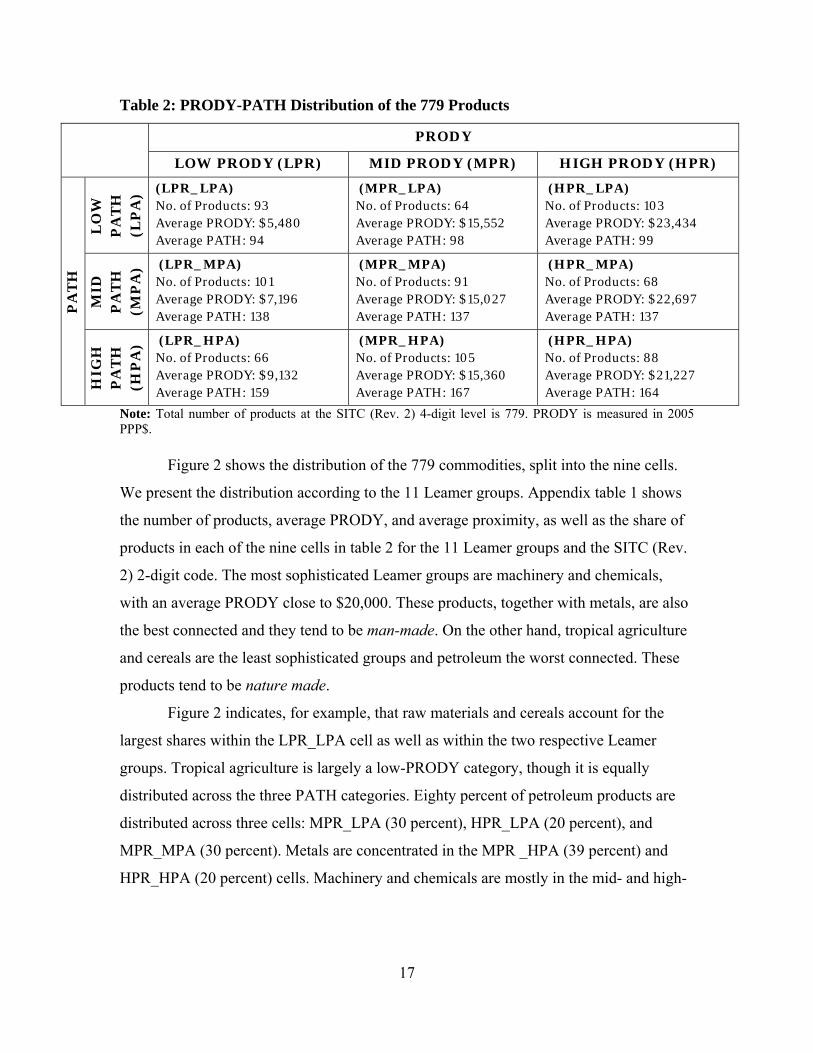
Based on the distribution of the products according to their sophistication

(PRODY), we classify all products into high-PRODY, mid-PRODY, or low-PRODY,

depending on whether they belong to the first, second, or third tercile of the PRODY

scale. Similarly, we classify each product as being high-PATH, mid-PATH, or low-

PATH. We then assign each product to one of the nine cells of the PRODY-PATH

matrix. Table 2 shows this matrix, which provides a summary of the information of the

products in each of the nine cells: the number of products in each cell, the average

PRODY, and average PATH of the products in each cell. It can be seen that PATH

increases as we move down across rows (but does not vary across columns for a given

row), while PRODY increases as one moves to the right across columns (but does not

vary across rows for a given column). Out of the 779 products that we work with, 352 (45

percent of the total) are in the four cells MPR_MPA, HPR_MPA, MPR_HPA,

HPR_HPA (“good” products), and 427 (55 percent of the total) in the other five cells

(“bad” products). It is worth noting that the LPR_LPA cell contains 93 products, most of

them cereals and raw materials. On the other hand, the cell HPR_HPA at the other

extreme contains 88 products, most of them machinery and chemicals.

17

Table 2: PRODY-PATH Distribution of the 779 Products

PRODY

LOW PRODY (LPR) MID PRODY (MPR) HIGH PRODY (HPR)

LO

W

PA

TH

(L

PA

) (LPR_LPA) No. of Products: 93 Average PRODY: $5,480 Average PATH: 94

(MPR_LPA) No. of Products: 64 Average PRODY: $15,552 Average PATH: 98

(HPR_LPA) No. of Products: 103 Average PRODY: $23,434 Average PATH: 99

MID

P

AT

H

(MP

A) (LPR_MPA)

No. of Products: 101 Average PRODY: $7,196 Average PATH: 138

(MPR_MPA) No. of Products: 91 Average PRODY: $15,027 Average PATH: 137

(HPR_MPA) No. of Products: 68 Average PRODY: $22,697 Average PATH: 137 P

AT

H

HIG

H

PA

TH

(H

PA

) (LPR_HPA) No. of Products: 66 Average PRODY: $9,132 Average PATH: 159

(MPR_HPA) No. of Products: 105 Average PRODY: $15,360 Average PATH: 167

(HPR_HPA) No. of Products: 88 Average PRODY: $21,227 Average PATH: 164

Note: Total number of products at the SITC (Rev. 2) 4-digit level is 779. PRODY is measured in 2005 PPP$.

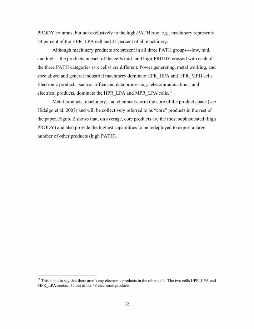
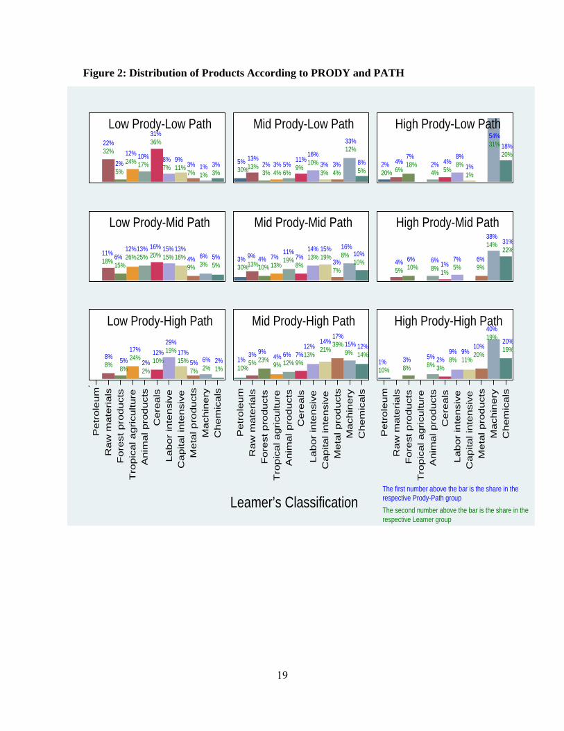
Figure 2 shows the distribution of the 779 commodities, split into the nine cells.

We present the distribution according to the 11 Leamer groups. Appendix table 1 shows

the number of products, average PRODY, and average proximity, as well as the share of

products in each of the nine cells in table 2 for the 11 Leamer groups and the SITC (Rev.

2) 2-digit code. The most sophisticated Leamer groups are machinery and chemicals,

with an average PRODY close to $20,000. These products, together with metals, are also

the best connected and they tend to be man-made. On the other hand, tropical agriculture

and cereals are the least sophisticated groups and petroleum the worst connected. These

products tend to be nature made.

Figure 2 indicates, for example, that raw materials and cereals account for the

largest shares within the LPR_LPA cell as well as within the two respective Leamer

groups. Tropical agriculture is largely a low-PRODY category, though it is equally

distributed across the three PATH categories. Eighty percent of petroleum products are

distributed across three cells: MPR_LPA (30 percent), HPR_LPA (20 percent), and

MPR_MPA (30 percent). Metals are concentrated in the MPR _HPA (39 percent) and

HPR_HPA (20 percent) cells. Machinery and chemicals are mostly in the mid- and high-

18

PRODY columns, but not exclusively in the high-PATH row, e.g., machinery represents

54 percent of the HPR_LPA cell and 31 percent of all machinery.

Although machinery products are present in all three PATH groups—low, mid,

and high—the products in each of the cells mid- and high-PRODY crossed with each of

the three PATH categories (six cells) are different. Power generating, metal working, and

specialized and general industrial machinery dominate HPR_HPA and HPR_MPH cells.

Electronic products, such as office and data processing, telecommunications, and

electrical products, dominate the HPR_LPA and MPR_LPA cells.12

Metal products, machinery, and chemicals form the core of the product space (see

Hidalgo et al. 2007) and will be collectively referred to as “core” products in the rest of

the paper. Figure 2 shows that, on average, core products are the most sophisticated (high

PRODY) and also provide the highest capabilities to be redeployed to export a large

number of other products (high PATH).

12 This is not to say that there aren’t any electronic products in the other cells. The two cells HPR_LPA and MPR_LPA contain 35 out of the 48 electronic products.

19

Figure 2: Distribution of Products According to PRODY and PATH

Pe

tro

leu

mR

aw

mate

rials

Fo

rest

pro

du

cts

Tro

pic

al a

gricu

lture

An

ima

l pro

du

cts

Cere

als

Labor

inte

nsi

veC

apita

l inte

nsi

veM

eta

l pro

du

cts

Mach

inery

Chem

icals

Low Prody-Low Path Mid Prody-Low Path High Prody-Low Path

Low Prody-Mid Path Mid Prody-Mid Path High Prody-Mid Path

Low Prody-High Path Mid Prody-High Path High Prody-High Path

Leamer’s Classification

Pe

tro

leu

mR

aw

mate

rials

Fo

rest

pro

du

cts

Tro

pic

al a

gricu

lture

An

ima

l pro

du

cts

Cere

als

Labor

inte

nsi

veC

apita

l inte

nsi

veM

eta

l pro

du

cts

Mach

inery

Chem

icals

Pe

tro

leu

mR

aw

mate

rials

Fo

rest

pro

du

cts

Tro

pic

al a

gricu

lture

An

ima

l pro

du

cts

Cere

als

Labor

inte

nsi

veC

apita

l inte

nsi

veM

eta

l pro

du

cts

Mach

inery

Chem

icals

The first number above the bar is the share in the respective Prody-Path groupThe second number above the bar is the share in the respective Leamer group

22%32%

2%5%

12%24%

10%17%

31%36%

8%7%

9%11% 3%

7%1%1%

3%3%

11%18% 6%

15%

12%26%

13%25%

16%20%

15%15%

13%18% 4%

9%6%3%

5%5%

8%8% 5%

8%

17%24%

2%2%

12%10%

29%19% 17%

15% 5%7%

6%2%

2%1%

13%13% 2%

3%3%4%

5%6%

11%9%

16%10% 3%

3%3%4%

33%12%

8%5%

5%30%

9%13%

4%10%

7%13%

11%19% 7%

8%

14%13%

15%19%

3%7%

16%8% 10%

10%3%30%

3%5%

9%23% 4%

9%6%12%

7%9%

12%13%

14%21%

17%39% 15%

9%12%14%

1%10%

4%6%

7%18% 2%

4%4%5%

8%8% 1%

1%

54%31% 18%

20%2%20%

4%5%

6%10%

6%8% 1%

1%

7%5%

6%9%

38%14% 31%

22%

1%10%

3%8%

5%8%

2%3%

9%8%

10%20%

40%19% 20%

19%9%11%

 

20

Forest products are equally distributed across the nine cells. Given that PRODY is

calculated using GDP per capita, and since some high-income countries such as Canada

export forest products, the sophistication level of some these products can come out to be

high.

Labor-intensive products are predominantly in four cells—low- and mid-PRODY

products crossed with mid- and high-PATH categories. Labor-intensive products in the

low-PRODY categories are mainly apparel, footwear, travel goods, and handbag

products. Labor-intensive products in the mid-PRODY category are mainly nonmetallic

mineral products and miscellaneous manufactures. Some of the nonmetallic minerals are

also in the high-PATH cells crossed with high- and mid-PRODY. Lastly, textiles account

for the presence of capital-intensive products in the four cells obtained from the cross of

mid- and low-PRODY with mid- and high-PATH categories.

3.2 Country Classification

Next, we classify countries according to the kind of the products they export with RCA

(an indicator of the kind of capabilities that a country has accumulated). To do so, we

calculate for each country the share of products exported with RCA (as percentage of the

country’s total number of products exported with RCA) that belong to each of the nine

cells in table 2. We assign each country to the cell with the largest share.

The LPR_MPH and MPR_HPA cells contain the largest number of countries, 86

and 25, respectively.13 Closer inspection shows that there is considerable heterogeneity

among countries within these two cells. For this reason, we split all countries into two

groups according to the share of core commodities exported with RCA in the total

number of commodities exported with RCA. “High-core” countries are those where the

share of core commodities exported with RCA in the total number of commodities

exported with RCA is above 30 percent.14 “Low-core” countries are those where the

share is less than 30 percent. As argued above, “core commodities” are, on average, the

13 The number of countries in the other cells is as follows: HPR_HPA, 9; HPR-MPA, 3; HPR_LPA, 2; MPR_MPA, 11; MPR_LPA, 0; LPR_HPA, 5; and LPR_LPA, 13. 14 Of the 779 commodities at the 4-digit SITC (Rev. 2) level of disaggregation, 41.1 percent (i.e., 320) are core commodities.

21

most sophisticated and the ones with the highest PATH. Countries that export a

significant share of core commodities face very different prospect from those of countries

with a low presence in the core. Tables 3 and 4 show the results. Appendix tables 2 and 3

show, for each of the 154 countries, the percentage of products exported with RCA in

each of the nine cells (of table 2), the total number of products exported with RCA, and

the share of core products in the total number of products exported with RCA . This

allows us to classify all 154 countries into four groups.

Table 3 (high-core countries, a total of 62) shows that there are no countries in the

LPR_LPA and MPR_LPA cells. This is an expected result because these are high-core

countries, i.e., countries where at least 30 percent of the commodities exported with RCA

are core commodities. The 34 countries in the HPR_HPA, HPR_MPA, MPR_MPA, and

MPR_HPA cells are mostly high-income countries. These countries are well-positioned.

The 28 countries in the HPR_LPA (2 countries), LPR_MPA (24 countries), and

LPR_HPA (2 countries) cells belong to what we refer to as the “middle product” trap.

Countries like China, India, Brazil, Mexico, Russia, Thailand, and Malaysia fall into this

group.

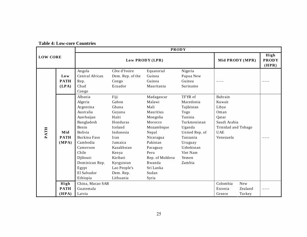
Table 4 (low-core countries, a total of 92) shows that there is no single country in

the high PRODY column as well as in the MPR_LPA cell. This is to be expected as

countries in this table are low core. Many of the oil-rich countries are in this table in the

MPR_MPA cell (9 countries). These countries, together with those in the MPR_HPA (5

countries) and in the LPR_HPA (3 countries), also suffer from a “middle-low product”

trap.15 Finally, a large number of low-core countries are in the LPR_LPA and in the

LPR_MPA cells (a total of 75 countries), i.e., their exports are concentrated in products

with low sophistication and little or average linkages with the other products. These

countries are in what we refer to as the “low product” trap. 16

15 By “worse position” we mean from the point of view of structural transformation. The cell MPR_MPA in table 4 for the low-core countries contains relatively rich oil exporters. 16 This simple criterion is not exempt of problems. While the classification of countries is easy, and in most cases the results were what one would expect a priori, it produced several cases difficult to explain. For example, high-income countries, like Australia and Iceland, are classified as LPR_MPA countries (table 4) alongside low-income countries. In contrast, Sierra Leone is classified as a MPR_HPA country along with high-income countries, such as France, the Netherlands, and Spain (table 3).

22

Collectively, we refer to the countries in the three traps as being in a “bad

product” trap, as they mostly export unsophisticated and unconnected products.17

Escaping the “bad product” trap is not straightforward or automatic. This will require

policy interventions to address market failures, many of which are prevalent in

developing countries.

Finally, appendix table 3 provides detailed information on 16 countries that we

have selected to shed light on why countries are classified in a specific cell, and why they

are in the trap. It shows the distribution of the total number of commodities exported with

RCA across the nine cells (of table 2) for the 11 Leamer categories. These countries are:

(i) High-core countries in the middle-product trap: Brazil, China, India, Malaysia,

and Thailand

All these are relatively advanced countries with a significant presence in core products,

although they also export a significant share of not too sophisticated and not too well-

connected commodities with comparative advantage.18 China’s presence in machinery is

mostly in electrical, office, and data-processing products, as well as telecommunication

products. India has significant presence in heavy machinery, and Brazil in heavy

machinery and vehicles. Malaysia and Thailand also have a significant presence in core

products largely due to the sophisticated goods they export in the machinery sector.

However, as shown in appendix table 3, most of these products are low- or mid-PATH

products.

17 We also tried an alternative classification of countries. In this alternative, we first classify countries according to sophistication (PRODY) and PATH, as above. However, PATH is now defined to include only linkages outside the product’s SITC 2-digit code, instead of including linkages to all products (i.e., including those within the same SITC 2-digit code). We find that the distribution of commodities in the nine cells is very similar to the one shown in table 2 (figure 2): 709 out of the 779 products belong to the same cell as in table 2 (figure 2). Also, the classification of countries in tables 3 and 4 does not change. 18 For detailed studies of China and India, see Felipe et al. (2010) and Felipe, Kumar, and Abdon (2010), respectively.

23

(ii) Low-core countries in the “low product” trap: Algeria, Australia, Bangladesh,

Chile, Nigeria, and Rwanda

Algeria and Nigeria export very few products with RCA, 20 and 28, respectively, and

they have very little presence in core products (6 and 4 commodities, respectively).

Limited capabilities, as well as a limited presence in core products, indicate that the

current economic structure of these two countries presents them with limited

opportunities to escape the low-product trap.

Bangladesh and Rwanda are better off, as they export a significantly higher

number of products, 81 and 69 products, respectively, with RCA, but only 6 and 12,

respectively, are core products; moreover, they do not have a presence in the high-

PRODY and high- and mid-PATH categories. Bangladesh’s exports are mainly labor-

intensive products (in Leamer’s classification), 50 percent of which are in the low-

PRODY–high-PATH cell. A closer inspection reveals that the high linkage of labor-

intensive products (specifically, apparels) is with machinery (specifically, electronics).

24

Table 3: High-core Countries

PRODY HIGH CORE

Low PRODY (LPR) Mid PRODY(MPR) High PRODY (HPR) Low

PATH (LPA)

––– ––– Guinea-Bissau Malaysia

Mid PATH (MPA)

Armenia Belize Brazil Burundi China Cyprus Gambia Georgia Hong Kong India Israel Jordan Lebanon

Liberia Mexico Niger Panama Philippines Russia Saint Kitts, Nevis and Anguilla Samoa Senegal South Africa Thailand

Malta Republic of Korea

Ireland Japan Singapore

PA

TH

High PATH (HPA)

Bulgaria Ukraine

Barbados Belarus Belgium Bosnia Herzegovina Canada Costa Rica Croatia Czech Rep. France Hungary Italy

Netherlands Poland Portugal Romania Seychelles Sierra Leone Slovakia Slovenia Spain

Austria Denmark Finland Germany Norway Sweden Switzerland USA United Kingdom

25

Table 4: Low-core Countries PRODY

LOW CORE Low PRODY (LPR) Mid PRODY (MPR)

High PRODY (HPR)

Low PATH (LPA)

Angola Central African Rep. Chad Congo

Côte d'Ivoire Dem. Rep. of the Congo Ecuador

Equatorial Guinea Guinea Mauritania

Nigeria Papua New Guinea Suriname

––– –––

Mid PATH (MPA)

Albania Algeria Argentina Australia Azerbaijan Bangladesh Benin Bolivia Burkina Faso Cambodia Cameroon Chile Djibouti Dominican Rep. Egypt El Salvador Ethiopia

Fiji Gabon Ghana Guyana Haiti Honduras Iceland Indonesia Iran Jamaica Kazakhstan Kenya Kiribati Kyrgyzstan Lao People's Dem. Rep. Lithuania

Madagascar Malawi Mali Mauritius Mongolia Morocco Mozambique Nepal Nicaragua Pakistan Paraguay Peru Rep. of Moldova Rwanda Sri Lanka Sudan Syria

TFYR of Macedonia Tajikistan Togo Tunisia Turkmenistan Uganda United Rep. of Tanzania Uruguay Uzbekistan Viet Nam Yemen Zambia

Bahrain Kuwait Libya Oman Qatar Saudi Arabia Trinidad and Tobago UAE Venezuela ––– P

AT

H

High PATH (HPA)

China, Macao SAR Guatemala Latvia

Colombia Estonia Greece

New Zealand Turkey

–––

26

Chile has been a regional powerhouse since the end of the nineteenth century and

for decades it has had a history of industrial policy. Agosin, Larrain, and Grau (2009)

note that the major thrust of the industrial policy framework in Chile is largely

“horizontal,” designed to resolve economy-wide market failures, improve productivity,

and raise the technological content of the existing sector. Although Chile does not have a

clear comparative advantage in manufactured goods, the industrial sector helped establish

an alternative sector, and the success of the Chilean salmon industry is an example of

how industrial policy can be used to resolve various market failures.

Australia is a rich country with a high income per capita. One key reason why

Australia, despite its strong tilt towards the primary sector, is a rich country (like some

other exporters of primary products) is that, aware of the dangers of specializing in the

production of raw materials, long ago it developed a national manufacturing sector, even

though it would never be able to compete with the industry of the advanced countries. It

was argued that an industrial sector would provide an alternative source of employment

and an alternative wage level that would signal that moving production to marginal lands

was not profitable. In addition, the industrial sector would help mechanize the production

of wool. This, of course, would not have happened without an active government support.

(iii) Low-core countries in the “middle-low product” trap: Saudi Arabia and the

United Arab Emirates

Saudi Arabia and the United Arab Emirates (UAE) are, like Algeria and Nigeria, oil

exporters. However, the former two countries have a much higher per capita income. One

reason is that they have a certain presence in core products (chemicals), although not as

significant as that of the middle-product countries. Also, in addition to natural resources,

what makes Saudi Arabia and the UAE (and some other oil-rich countries) rich is that

they have been able to develop the service sector.

(iv) High-core countries in the HPR_MPA cell: Ireland and Singapore

Both Singapore and Ireland export a significant number of core products with RCA, 37

(43 percent of the total) and 70 (62.5 percent of the total), respectively. Yet, a significant

27

share of their exports is not in the high-PATH cells. This makes it difficult for them to

jump to other, better-connected, and more sophisticated products. The success of

Singapore and Ireland must be understood in the context of the role played by industrial

policy. For example, Ireland’s take off in the 1980s had much to do with the government-

led strategy to succeed in the IT sector, adopted under Prime Minister Charles Haughey.

In the case of Singapore, industrial development has played a key role in the development

of the island state during the last 50 years, and the wide range of capabilities acquired as

a result of being a port has allowed it to venture into complex services.

(v) High-core countries in the HPR_HPA cell: Finland

In the 1950s, as much as 40 percent of Finland’s employment and output were in the

primary sector. The growth strategy adopted in the postwar period relied on government

intervention alongside the private sector to set up a strong manufacturing sector. Today,

Finland has a significant presence in core products. In the early 1990s, Nokia was a small

company getting out of the production of rubber boots and cement for tiles into

electronics. Nokia benefited enormously from Finland’s industrial policy programs.

4. POLICIES TO ESCAPE THE “BAD PRODUCT” TRAP

The analysis in previous sections has allowed us to classify all 154 countries into four

groups, depending on which export category (based on the PATH-PRODY analysis) is

the most important one. Accordingly, we propose policies for each of them. Necessarily,

the policies discussed are generic and, when made operational, they will have to become

country-specific.

A. High-core Countries That Are Exporters of “Good” Products (34 countries)

These are countries (table 3) with a high share of exports of core products, and,

moreover, these products are medium-high PRODY and medium-high PATH. Many of

these products: (i) are subject increasing returns to scale; (ii) have a high income

elasticity of export demand; and (iii) are produced under conditions of imperfect

28

competition. Our argument is that these countries became rich because they learned how

to export these types of products. To do this, they had to accumulate more and more of

the capabilities that are necessary to master these commodities. This was a path-

dependent process that started in the Middle Ages in some cases (e.g., United Kingdom)

and supported by a myriad of industrial policy actions, many of which would be illegal

today (Chang 2002).19 These countries need to continue upgrading through R&D and

improvements in the quality of their tertiary education.

The next three groups, comprising 120 of the 154 countries that we have

analyzed, are in need of different types of policies to move forward. These are the ones

that suffer from the “middle” or “low product” traps.

B. High-core Countries in the “Middle Product” Trap (28 countries)

These countries (table 3) are well-positioned to continue doing well. At least 30 percent

of the products that they export with RCA are core products. Many of the countries in the

so-called middle-income trap are in this group. The policies these countries require are of

two types, depending on the cell they lie in:

• Competitiveness policy for the two countries in the LPR_HPA cell: Focus on

quality upgrading of the existing products instead of jumps to new products.

• Soft parsimonious industrial policy for the twenty-four countries in the

LPR_MPA cell and for the two countries in the HPR_LPA cell:

o Facilitate horizontal jumps to nearby products.

o Develop a process whereby government, industry, and cluster-level private

organizations can collaborate on interventions that can directly increase

productivity.

o Focus on interventions that deal directly with the coordination problems

that keep productivity low in existing or raising sectors (e.g., programs

19 See Chang’s (2002) analysis of the United Kingdom, the United States, Germany, France, Sweden, Belgium, The Netherlands, Switzerland, Japan, and the NIEs.

29

and grants to help particular clusters by increasing the supply of skilled

workers; encourage technology adoption; improve regulation and

infrastructure).

C. Low-core Countries in the “Middle-low Product” Trap (17 countries)

The difference between these countries (table 4) and those in the previous group is a

matter of degree. Emphasis in these countries has to be toward increasing the number of

core products exported with RCA:

• Hard parsimonious industrial policy:20

o Facilitate horizontal jumps to far away products.

o Tariff exemptions, subsidies for infrastructure, etc. to develop an industry.

Back up all its public input needs plus some subsidies to get the private

sector going.

D. Low-core Countries in the “Low-product” Trap (75 countries)

Sadly, most countries in the world lie in this group (table 4).

• Many of the products exported by these countries are nature-made and subject to

decreasing returns. Only industrialization can create an effective agricultural

sector. None of these countries will ever get rich without an industrial and an

advanced service sector.

• In the traditional trap literature (à la Nelson and Myrdal) there were two ways to

escape from the low-level equilibrium trap. First, per capita income must be

raised, in one go, to the point where the trap would not force income per capita 20 These policies have to be consistent with World Trade Organization (WTO) rules. Amsden (2000) and Amsden and Hikino (2000) argue that the new rules of the WTO allow countries to promote their industries, including the manufacturing sector, in particular under the umbrella of advancing science and technology (e.g., by setting up technology parks). Subsidies in exchange for monitorable, results-oriented performance standards are acceptable. Countries can, for example, target national champions. The hurdles that developing countries face are the following: (i) informal political pressures by the developed countries in favor of market opening; (ii) the subjection of countries that make use of WTO rules to promote their industries to “reciprocal control mechanisms”; and (iii) their lack of “vision.”

30

down again to the subsistence level. Second, the growth rate of population must

decline (e.g., reduction in the birth rate or emigration), and/or that of national

income increase (e.g., through technical progress or capital from abroad).

Industrialization greatly increases a country’s ability to sustain a large population.

• To a certain extent and under this view, some of these countries may need a “big

push,” that is, a planned large-scale expansion of a wide range of economic

activities and achieve a “critical minimum effort” (investment requirements to

raise per capita income to the level beyond which the further growth of per capita

income will not be associated with income-depressing forces exceeding income-

raising forces).

• The above will not be enough: simply “pumping money” will not help unless a

critical mass in an increasing returns sector is created. These countries will need

their governments to take “strategic bets” by getting directly involved in the

development of new sectors (big leaps). This, however, will be difficult for many

countries in this group, as, by definition, they lack the required capabilities, as

defined in section 2.

• For this reason, it is imperative that these countries focus their efforts on

accumulating new capabilities. This will require: (i) human capital to acquire

skills, technology, and knowledge (in many cases, basic management, accounting,

and record keeping); (ii) a higher drive to diversify and to increase sophistication

by embracing a realistic industrial vision; and (iii) improvement in organizational

abilities (e.g., firm-level organization).

Many of the problems that affect countries in groups B, C, and D (in particular those in

the last group) above have been studied in the literature from different angles and provide

complementary insights to the work on structural transformation developed by Hidalgo et

al (2007). For example, Kremer’s (1993) O-Ring theory of development is an attempt at

explaining the large differences in income between developed and developing countries.

Kremer argued that production is often the result of a series of tasks, for example, on an

assembly line. These tasks can be performed at different levels of “skills,” which refer to

31

the probability of successfully completing the task. For the final product or service to be

successfully made or delivered, every single task must be completed correctly.21 This

implies that the value of each worker’s efforts depends on the quality of all other

workers’ efforts. Kremer’s theory explains why workers of similar skills have strong

incentives to match together, i.e., highly skilled workers will attempt to work with other

highly skilled workers, and low-skilled workers with other low-skilled workers. Highly

skilled workers complement each other, giving rise to increasing returns to skills and

even higher productivity; unskilled workers, when they match together, lower each

others’ productivity even more.22

O-ring effects also exist across firms. Suppose one firm builds roads and another

one automobiles. The additional value to drivers of an improvement in the quality of cars

most likely will be smaller if the roads happen to be of a poor quality, and vice versa.

When tasks are performed sequentially (as in global value chains), highly skilled workers

will perform the tasks at the later, more complex stages of production—which explains

why poor countries have higher shares of primary output in GDP—and workers will be

paid more in industries with high-value inputs. Also, under sequential production,

countries with highly skilled workers specialize in products that require expensive

intermediate goods, and countries with low-skill workers specialize in primary

production. In other words, nothing is natural about the international pattern of

specialization: comparative advantage in primary goods, manufactures, and services is

itself endogenously determined, or, in the words of Easterly: “Comparative advantage in

agriculture and manufactures is itself manufactured” (Easterly 2002: 161). The

21 An “o-ring” is a donut-shaped rubber seal. The malfunctioning of one such seal caused the explosion of the Challenger space shuttle in 1986. The shuttle had cost billions of dollars, required the cooperation of hundreds of teams, and combined a considerable number of components. All this joint effort was lost because one seal failed to function properly. 22 Kremer’s (1993) model explains why highly skilled workers, such as surgeons from India or the Philippines, want to migrate to the advanced countries, giving rise to brain drain. They will be much more productive after they have migrated, even though their individual skills remain the same. Migration allows them to match up with the skilled labor force of the developed country.22 The matching story also offers an explanation of income differences among countries. A small difference in workers’ skills leads to a proportionally larger difference in wages and output, so wages and productivity differentials between countries with different skill levels are enormous.

32

conclusion is that rich and skilled nations will produce “advanced” and “high-value”

goods” (or the final stages of a process in a global value chain), while the poor nations

will produce raw materials (primary production in general) and “low-value” goods.

Under these circumstances, the rich and skilled nations will produce “advanced”

and “high-value” goods” (or the final stages of a process in a global value chain), while

the poor nations will produce raw materials (primary production in general) and “low-

value” goods. This is also consistent with Lall’s (2000a) claim that export structures tend

to be path-dependent and difficult to change, which has important implications for

growth and development. Indeed, trade patterns are much less responsive to changing

factor prices than is commonly assumed. Export structures and trade patterns in general

are the outcome of a long, cumulative process of learning, agglomeration, increasing

returns, institution building, and business culture. This means that the world’s pattern of

specialization and trade is, fundamentally, arbitrary—what each country produces is the

result of history, accidents, and past government policies, and it is not dictated by

comparative advantage given by tastes, resources, and technology (also, Thirlwall and

Pacheco-López 2008).

In related work, Snower (1996) has argued that countries that try to progress by

exploiting low labor costs (e.g., by restricting wages or through devaluations) may end up

stuck in a vicious circle of low productivity, deficient training, and a lack of skilled jobs,

therefore preventing key sectors from competing effectively in the markets for skill-

intensive products. This situation is referred to as a “low-skill, bad-job trap.” “Bad jobs”

are associated with low wages and few opportunities to accumulate human capital. “Good

jobs” demand higher skills and command higher wages. Innovating is crucial for

developing technological capabilities, but it requires well-trained workers. Economies

can get caught in a vicious circle in which firms do not innovate because the labor force

is insufficiently skilled, and workers do not have incentives to invest in knowledge

because there is no demand for these skills. Snower (1996) argues that the relatively low

demand for and supply of skills in a country derives from rational decisions made by both

firms and individuals within the particular legal and institutional framework in which

they operate. Countries with a less-skilled workforce have greater incentives to produce

33

nontraded services rather than tradables such as manufactured goods because the former

are relatively protected from foreign competition. This pattern of specialization creates

and perpetuates the demand for less-skilled labor.

One of the most important consequences of the deficiency in training is that a lack

of skilled workers leads to the manufacture and export of relatively poor-quality and low-

value products. The manufacture of high-quality products requires highly trained

workers. But if the country does not generate enough of these workers, firms will be

forced to produce low-quality goods; likewise, workers will acquire little training because

few high-quality goods are produced, leading to a vicious circle. The choices made by

employers reflect the availability of a skilled workforce. Different outputs require

different types of training. Businesspeople aware that their workers are not highly skilled

(and thus are more likely to make mistakes) will tend to specialize in the production of

low-value products. Thus, the labor force will be more suited to the production of low-

value than high-value products. Why can this happen? The reason is that the market does

not lead to the best possible outcome because, as explained above, private and social

returns to knowledge are different. Individuals are not fully rewarded for the social

contribution they make when they invest in knowledge by increasing the stock of

knowledge available to everyone. They get no reward for this spillover, and so

contributions to social knowledge will be underprovided. In the end, firms’ decisions

about what type of products to manufacture depend on the availability of skilled labor.

The result is that “in countries that offer little support for education and training and that

contain a large proportion of unskilled workers, the market mechanism may reinforce the

existing lack of skills by providing little incentive to acquire more; whereas in countries

with well-functioning educational and training institutions and large bodies of skilled

labor, the free market may do much more to induce people to become skilled” (Snower

1996: 112).

Finally, Sutton (2001, 2005) has argued that if two countries differ in their levels

of capability, this will be reflected as a difference in their real wage levels. Low wages do

not compensate for low quality, with the consequence that the low-quality firms will be

excluded from the market. Indeed, one of the most important effects of globalization is

34

competition in “capability building.” This will lead to a shakeout of firms in low-

capability countries. Can capabilities be transferred? Maybe yes, but this is a slow,

expensive, and painstaking process,23 and from the point of view of a high-quality

producer moving to a low-wage country need not be optimal; first because it operates in

an environment where she relies on suppliers of intermediate inputs that probably are not

present in the low-wage country and, second, because the firm’s capabilities are

embodied in the tact knowledge possessed jointly by those individuals who comprise the

firm’s workforce.

5. CONCLUSIONS: IT’S THE ECONOMIC STRUCTURE…DUH!

In this paper we have argued that what sets apart countries is their productive structure

and the specific characteristics of the products that they export. These, in turn, depend on

the capabilities that the firms possess. Development in this paradigm is a process of

generating new activities and letting others disappear. The primary driver of growth is the

gradual build-up in firms’ capabilities, which raises the economy-wide real wage. Capital

accumulation is a complementary effect: the higher real wage makes it profitable for each

firm to shift to more capital-intensive techniques. As the firm makes that shift, the rise in

its capital-labor ratio further raises the marginal revenue product of labor at the firm

level, and so underpins the rising real wage.

Using measures of product sophistication and connectivity, we have shown that

not all products are the same. Using the SITC 4-digit level containing 779 products, we

have determined that 427 (about 55 percent) are not very sophisticated and/or not well-

connected to the other products. This has allowed us to split the 154 countries in our

analysis into four groups: (i) a group of 34 countries that export mostly “good” products.

These are sophisticated and well-connected products, and in general, are man-made; (ii) a

23 Sutton (2005) argues that a good proxy for the cost of transferring a capability is given by counting the number of individuals that are needed to assemble in order to form a sufficient subset of employees who can carry the capability. The important things that must be transferred relate not so much to items that can be successfully reduced to a statement in a manual, but rather to complex and interrelated patterns of working practices that are extremely difficult and time-consuming to unravel and redesign.

35

group of 28 countries that export a significant share of core products, although not as

sophisticated and well-connected as those exported by the countries in the previous

group. These countries are in a “middle product” trap; (iii) a group of 17 countries that

export few core products. They export products of that are in the middle of the

sophistication and connectedness scale. They are in a “middle-low product trap”; and (iv)

a large group of 75 countries that mostly export unsophisticated and poorly-connected

products. They are in a “low-product” trap. Countries in these two groups specialize in

nature-made products, subject to decreasing returns to scale.

The policies that the countries in the last three groups require range from

competitiveness and soft parsimonious industrial policy to aggressive policies that lead to

the rapid accumulation of relevant capabilities, as well as strategic bets with significant

government intervention. Historically, it has been impossible to become a rich country

without creating an industrial sector and an advanced service sector. Likewise,

historically, no country has become rich without explicit government interventions that

amount to industrial policy in different shapes and forms.

36

BIBLIOGRAPHY Aghion, P. and P. Howitt. 1998. Endogenous Growth Theory. Cambridge, MA: MIT

Press. Agosin, M., C. Larrain, and N. Grau. 2009. “Industrial Policy in Chile.” Working Paper

294. Santiago: Department of Economics, University of Chile. Amsden, A. 2000. “Industrialization under WTO Law.” Available at: www.unctad-

10.org/pdfs/ux_tdxrt1d7.en.pdf Amsden, A. and T. Hikino. 2000. “The Bark Is Worse Than the Bite: New WTO Law

and Late Industrialization.” American Academy of Political and Social Science. 570 (July): 104–14.

Balassa, B. 1965. “Trade Liberalization and Revealed Comparative Advantage.”

Manchester School of Economics and Social Studies 33: 99–123. Barro, R., and X. Sala-i-Martin. 1995. Economic Growth. New York: McGraw-Hill. Blomstrom, M., R. Lipsey, and M. Zejan. 1996. “Is Fixed Investment the Key to

Economic Growth?” The Quarterly Journal of Economics 111(1): 269–76. Chang, Ha-Joon. 2002. Kicking Away the Ladder. London: Anthem Press. Chenery, H., S. Robinson, and M. Syrquin (eds.). 1986. Industrialization and growth: A

comparative study. New York: Oxford University Press. De Ferranti, D., G.E. Perry, I.S. Gill., and L. Severn. 2000. Securing our future in a

global economy. Washington, DC: The World Bank. Domar, E. 1946. “Capital Expansion, Rate of Growth and Employment.” Econometrica

14: 137–47. Easterly, W. 2002. The Elusive Quest for Growth: Economists’ Adventures and

Misadventures in the Tropics. Cambridge, MA: MIT Press. Felipe, J., U. Kumar, N. Usui, and A. Abdon. 2010. “Why has China succeeded? And

Why it Will Continue to Do So.” Working Paper 611. Annandale-on-Hudson, NY: Levy Economics Institute of Bard College.

Felipe, J., U. Kumar, and A. Abdon. 2010. “Exports, Capabilities, and Industrial Policy in

India.” Mimeograph. Manila: Asian Development Bank.

37

Felipe, J., M. León-Ledesma, M. Lanzafame, and G. Estrada. 2009. “Sectoral Engines of Growth in Developing Asia: Stylized Facts and Implications.” Malaysian Journal of Economic Studies 46(2): 107–33.

Harrod, R. 1939. “An Essay in Dynamic Theory.” The Economic Journal 49: 14–33. Hausmann, R., and B. Klinger. 2007. “The Structure of the Product Space and the

Evolution of Comparative Advantage.” Working Paper 146. Cambridge, MA: Center for International Development, Harvard University.

————. 2006. “The Structure of the Product Space and the Evolution of Comparative

Advantage.” Working Paper 128. Cambridge, MA: Center for International Development, Harvard University.

Hausmann, R., and D. Rodrik. 2003. “Economic Development as Self-discovery.”

Journal of Development Economics 72(2): 603–33. Hausmann, R., J. Hwang, and D. Rodrik. 2007. “What you export matters.” Journal of

Economic Growth 12(1): 1–15.

Hidalgo, C., B. Klinger, A.L. Barabasi, and R. Hausmann. 2007. “The Product Space Conditions the Development of Nations.” Science 317: 482–7.

Kaldor, N. 1967. Strategic Factors in Economic Development. Ithaca, NY: New York

State School of Industrial and Labor Relations, Cornell University. ————. 1970. “The Case for Regional Policies.” Scottish Journal of Political

Economy 17(3): 337–48. Kremer, M. 1993. “The O-Ring Theory of Economic Development.” The Quarterly

Journal of Economics 108: 551–75. Kuznet, S. 1966. Modern Economic Growth. New Haven, CT: Yale University

Press. Lall, S. 1992. “Technological Capabilities and Industrialization.” World Development

20(2): 165–86. ————. 2000a. “The Technological Structure and Performance of Developing Country

Manufactured Exports, 1985–98.” Oxford Development Studies 28(3): 337–69.

38

————. 2000b. “Technological Change and Industrialization in the Asian Newly Industrializing Economies: Achievements and Challenges.” in L. Lim and R. Nelson (eds.), Technology, Learning and Innovation: Experiences of Newly Industrializing Economies. Cambridge, UK: Cambridge University Press.

Lall, S., M. Albaladejo, and J. Zhang. 2004. “Mapping Fragmentation: Electronics and

Automobiles in East Asia and Latin America.” Oxford Development Studies 32(3): 407–32.

Lall, S., J. Weiss, and J. Zhang. 2006. “The ‘sophistication’ of exports: A new trade

measure.” World Development 34(2): 222–37. Leamer, E. 1984. Sources of International Comparative Advantage: Theory and

Evidence. Cambridge, MA: MIT Press. Lewis, A. 1955. The Theory of Economic Growth. Homewood, IL: Irwin. Lucas, R. 1988. “On the Mechanics of Economic Development.” Journal of Monetary

Economics 22: 3–42. Myrdal, G. 1957. Economic Theory and Under-Developed Regions. London: Duckworth. Nelson, R. 1956. “A Theory of the Low-Level Equilibrium Trap in Underdeveloped

Economies.” American Economic Review 46(5): 894–908. Oulton, N., and M. O’Mahony. 1994. Productivity and Growth: A Disaggregated Study

of British Industry, 1954–86. Cambridge, UK: Cambridge University Press. Prichett, L. 2003. “A Conclusion to Cross-National Growth Research: A Foreword ‘To

the Countries Themselves’.” in Gary McMahon and Lyn Squire (eds.), Explaining Growth. London: Palgrave Macmillan.

Rodrik, D. 2004. “Industrial Policy for the 21st Century.” Discussion Paper 4767.

Washington, DC: Center for Economic and Policy Research (CEPR). Snower, D. 1996. “The low-skill, bad-job trap.” in A. Booth and D. Snower (eds.),

Acquiring Skills: Market Failures, their Symptoms and Policy Responses. Cambridge, UK: Cambridge University Press.

Solow, R. 1956. “A Contribution to the Theory of Economic Growth.” Quarterly Journal

of Economics 70: 65–94. Sutton, J. 2005. 2001. “Rich Trades, Scarce Capabilities: Industrial Development

Revisited.” Keynes Lecture, British Academy 2000.

39

————. “Competing in Capabilities: An Informal Overview.” Manuscript, April 25. London: London School of Economics.

Thirlwall, A., and P. Pacheco-Lopez. 2008. Trade Liberalisation and the Poverty of

Nations. Cheltenham: Edward Elgar.

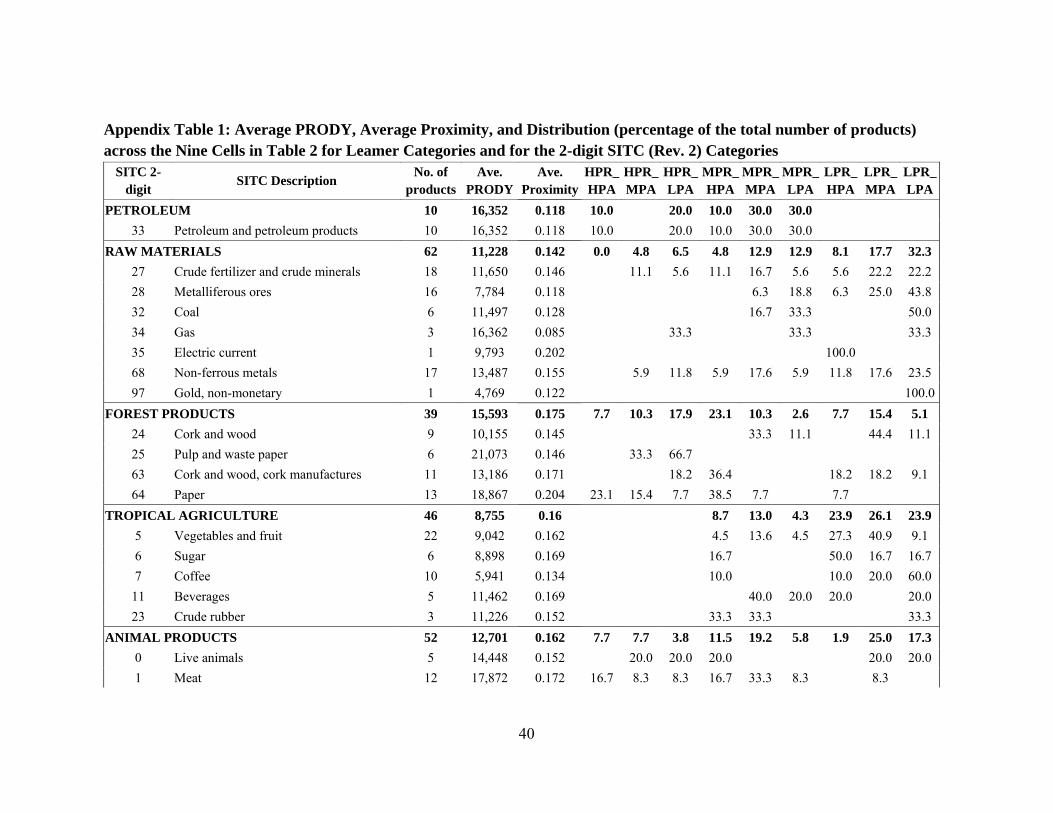
40

Appendix Table 1: Average PRODY, Average Proximity, and Distribution (percentage of the total number of products) across the Nine Cells in Table 2 for Leamer Categories and for the 2-digit SITC (Rev. 2) Categories

SITC 2-digit

SITC Description No. of

productsAve.

PRODYAve.

ProximityHPR_HPA

HPR_MPA

HPR_LPA

MPR_HPA

MPR_MPA

MPR_LPA

LPR_HPA

LPR_MPA

LPR_LPA

PETROLEUM 10 16,352 0.118 10.0 20.0 10.0 30.0 30.0 33 Petroleum and petroleum products 10 16,352 0.118 10.0 20.0 10.0 30.0 30.0

RAW MATERIALS 62 11,228 0.142 0.0 4.8 6.5 4.8 12.9 12.9 8.1 17.7 32.3 27 Crude fertilizer and crude minerals 18 11,650 0.146 11.1 5.6 11.1 16.7 5.6 5.6 22.2 22.2 28 Metalliferous ores 16 7,784 0.118 6.3 18.8 6.3 25.0 43.8 32 Coal 6 11,497 0.128 16.7 33.3 50.0 34 Gas 3 16,362 0.085 33.3 33.3 33.3 35 Electric current 1 9,793 0.202 100.0 68 Non-ferrous metals 17 13,487 0.155 5.9 11.8 5.9 17.6 5.9 11.8 17.6 23.5 97 Gold, non-monetary 1 4,769 0.122 100.0

FOREST PRODUCTS 39 15,593 0.175 7.7 10.3 17.9 23.1 10.3 2.6 7.7 15.4 5.1 24 Cork and wood 9 10,155 0.145 33.3 11.1 44.4 11.1 25 Pulp and waste paper 6 21,073 0.146 33.3 66.7 63 Cork and wood, cork manufactures 11 13,186 0.171 18.2 36.4 18.2 18.2 9.1 64 Paper 13 18,867 0.204 23.1 15.4 7.7 38.5 7.7 7.7

TROPICAL AGRICULTURE 46 8,755 0.16 8.7 13.0 4.3 23.9 26.1 23.9 5 Vegetables and fruit 22 9,042 0.162 4.5 13.6 4.5 27.3 40.9 9.1 6 Sugar 6 8,898 0.169 16.7 50.0 16.7 16.7 7 Coffee 10 5,941 0.134 10.0 10.0 20.0 60.0

11 Beverages 5 11,462 0.169 40.0 20.0 20.0 20.0 23 Crude rubber 3 11,226 0.152 33.3 33.3 33.3

ANIMAL PRODUCTS 52 12,701 0.162 7.7 7.7 3.8 11.5 19.2 5.8 1.9 25.0 17.3 0 Live animals 5 14,448 0.152 20.0 20.0 20.0 20.0 20.0 1 Meat 12 17,872 0.172 16.7 8.3 8.3 16.7 33.3 8.3 8.3

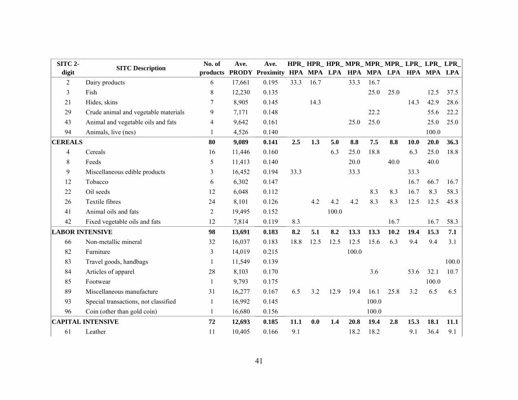
41

SITC 2-digit

SITC Description No. of

productsAve.

PRODYAve.

ProximityHPR_HPA

HPR_MPA

HPR_LPA

MPR_HPA

MPR_MPA

MPR_LPA

LPR_HPA

LPR_MPA

LPR_LPA

2 Dairy products 6 17,661 0.195 33.3 16.7 33.3 16.7 3 Fish 8 12,230 0.135 25.0 25.0 12.5 37.5

21 Hides, skins 7 8,905 0.145 14.3 14.3 42.9 28.6 29 Crude animal and vegetable materials 9 7,171 0.148 22.2 55.6 22.2 43 Animal and vegetable oils and fats 4 9,642 0.161 25.0 25.0 25.0 25.0 94 Animals, live (nes) 1 4,526 0.140 100.0

CEREALS 80 9,089 0.141 2.5 1.3 5.0 8.8 7.5 8.8 10.0 20.0 36.3 4 Cereals 16 11,446 0.160 6.3 25.0 18.8 6.3 25.0 18.8 8 Feeds 5 11,413 0.140 20.0 40.0 40.0 9 Miscellaneous edible products 3 16,452 0.194 33.3 33.3 33.3

12 Tobacco 6 6,302 0.147 16.7 66.7 16.7 22 Oil seeds 12 6,048 0.112 8.3 8.3 16.7 8.3 58.3 26 Textile fibres 24 8,101 0.126 4.2 4.2 4.2 8.3 8.3 12.5 12.5 45.8 41 Animal oils and fats 2 19,495 0.152 100.0 42 Fixed vegetable oils and fats 12 7,814 0.119 8.3 16.7 16.7 58.3

LABOR INTENSIVE 98 13,691 0.183 8.2 5.1 8.2 13.3 13.3 10.2 19.4 15.3 7.1 66 Non-metallic mineral 32 16,037 0.183 18.8 12.5 12.5 12.5 15.6 6.3 9.4 9.4 3.1 82 Furniture 3 14,019 0.215 100.0 83 Travel goods, handbags 1 11,549 0.139 100.084 Articles of apparel 28 8,103 0.170 3.6 53.6 32.1 10.7 85 Footwear 1 9,793 0.175 100.0 89 Miscellaneous manufacture 31 16,277 0.167 6.5 3.2 12.9 19.4 16.1 25.8 3.2 6.5 6.5 93 Special transactions, not classified 1 16,992 0.145 100.0 96 Coin (other than gold coin) 1 16,680 0.156 100.0

CAPITAL INTENSIVE 72 12,693 0.185 11.1 0.0 1.4 20.8 19.4 2.8 15.3 18.1 11.1 61 Leather 11 10,405 0.166 9.1 18.2 18.2 9.1 36.4 9.1

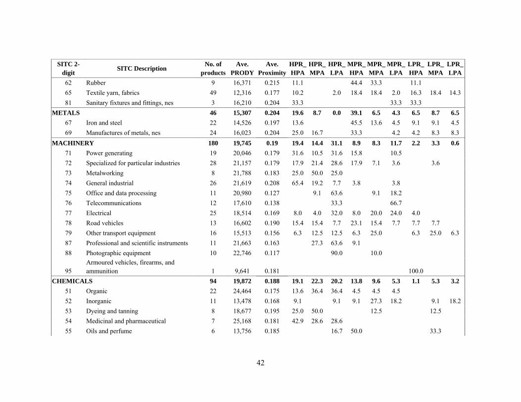
42

SITC 2-digit

SITC Description No. of

productsAve.

PRODYAve.

ProximityHPR_HPA

HPR_MPA

HPR_LPA

MPR_HPA

MPR_MPA

MPR_LPA

LPR_HPA

LPR_MPA

LPR_LPA

62 Rubber 9 16,371 0.215 11.1 44.4 33.3 11.1 65 Textile yarn, fabrics 49 12,316 0.177 10.2 2.0 18.4 18.4 2.0 16.3 18.4 14.3 81 Sanitary fixtures and fittings, nes 3 16,210 0.204 33.3 33.3 33.3

METALS 46 15,307 0.204 19.6 8.7 0.0 39.1 6.5 4.3 6.5 8.7 6.5 67 Iron and steel 22 14,526 0.197 13.6 45.5 13.6 4.5 9.1 9.1 4.5 69 Manufactures of metals, nes 24 16,023 0.204 25.0 16.7 33.3 4.2 4.2 8.3 8.3

MACHINERY 180 19,745 0.19 19.4 14.4 31.1 8.9 8.3 11.7 2.2 3.3 0.6 71 Power generating 19 20,046 0.179 31.6 10.5 31.6 15.8 10.5 72 Specialized for particular industries 28 21,157 0.179 17.9 21.4 28.6 17.9 7.1 3.6 3.6 73 Metalworking 8 21,788 0.183 25.0 50.0 25.0 74 General industrial 26 21,619 0.208 65.4 19.2 7.7 3.8 3.8 75 Office and data processing 11 20,980 0.127 9.1 63.6 9.1 18.2 76 Telecommunications 12 17,610 0.138 33.3 66.7 77 Electrical 25 18,514 0.169 8.0 4.0 32.0 8.0 20.0 24.0 4.0 78 Road vehicles 13 16,602 0.190 15.4 15.4 7.7 23.1 15.4 7.7 7.7 7.7 79 Other transport equipment 16 15,513 0.156 6.3 12.5 12.5 6.3 25.0 6.3 25.0 6.3 87 Professional and scientific instruments 11 21,663 0.163 27.3 63.6 9.1 88 Photographic equipment 10 22,746 0.117 90.0 10.0

95 Armoured vehicles, firearms, and ammunition 1 9,641 0.181 100.0

CHEMICALS 94 19,872 0.188 19.1 22.3 20.2 13.8 9.6 5.3 1.1 5.3 3.2 51 Organic 22 24,464 0.175 13.6 36.4 36.4 4.5 4.5 4.5 52 Inorganic 11 13,478 0.168 9.1 9.1 9.1 27.3 18.2 9.1 18.2 53 Dyeing and tanning 8 18,677 0.195 25.0 50.0 12.5 12.5 54 Medicinal and pharmaceutical 7 25,168 0.181 42.9 28.6 28.6 55 Oils and perfume 6 13,756 0.185 16.7 50.0 33.3

43

SITC 2-digit

SITC Description No. of

productsAve.

PRODYAve.

ProximityHPR_HPA

HPR_MPA

HPR_LPA

MPR_HPA

MPR_MPA

MPR_LPA

LPR_HPA

LPR_MPA

LPR_LPA

56 Fertilizers 4 10,867 0.151 25.0 25.0 25.0 25.0 57 Explosives 3 14,486 0.152 33.3 33.3 33.3 58 Artificial resins and plastic 23 21,815 0.183 30.4 26.1 26.1 8.7 4.3 4.3 59 Chemical materials, nes 10 18,473 0.189 20.0 10.0 10.0 50.0 10.0

Note: HPR_HPA-High PRODY-High PATH; HPR_MPA-High PRODY-Mid PATH; HPR_LPA-High PRODY-Low PATH; MPR_HPA-Mid PRODY-High PATH; MPR_MPA-Mid PRODY-Mid PATH; MPR_LPA-Mid PRODY-Low PATH LPR_HPA-Low PRODY-High PATH; LPR_MPA-Low PRODY-Mid PATH; LPR_LPA-Low PRODY-Low PATH.

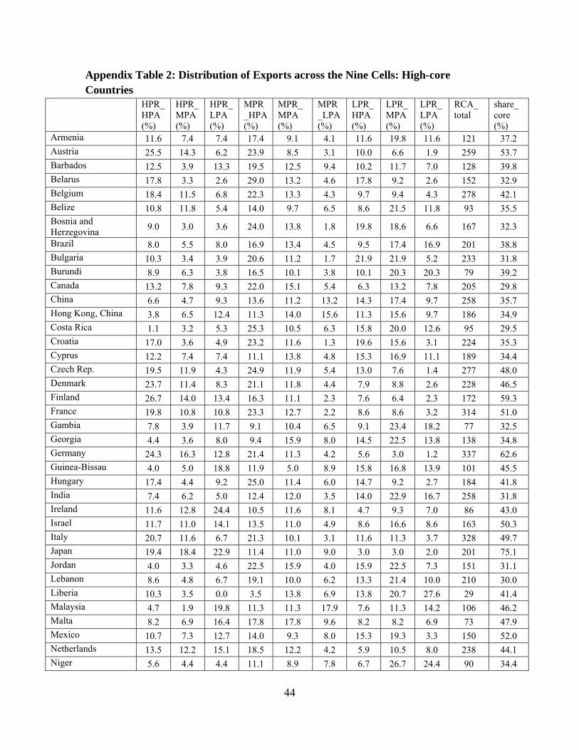
44

Appendix Table 2: Distribution of Exports across the Nine Cells: High-core Countries

HPR_HPA (%)

HPR_MPA (%)

HPR_LPA (%)

MPR_HPA (%)

MPR_MPA (%)

MPR_LPA (%)

LPR_HPA (%)

LPR_MPA (%)

LPR_LPA (%)

RCA_ total

share_ core (%)

Armenia 11.6 7.4 7.4 17.4 9.1 4.1 11.6 19.8 11.6 121 37.2 Austria 25.5 14.3 6.2 23.9 8.5 3.1 10.0 6.6 1.9 259 53.7 Barbados 12.5 3.9 13.3 19.5 12.5 9.4 10.2 11.7 7.0 128 39.8 Belarus 17.8 3.3 2.6 29.0 13.2 4.6 17.8 9.2 2.6 152 32.9 Belgium 18.4 11.5 6.8 22.3 13.3 4.3 9.7 9.4 4.3 278 42.1 Belize 10.8 11.8 5.4 14.0 9.7 6.5 8.6 21.5 11.8 93 35.5 Bosnia and Herzegovina 9.0 3.0 3.6 24.0 13.8 1.8 19.8 18.6 6.6 167 32.3

Brazil 8.0 5.5 8.0 16.9 13.4 4.5 9.5 17.4 16.9 201 38.8 Bulgaria 10.3 3.4 3.9 20.6 11.2 1.7 21.9 21.9 5.2 233 31.8 Burundi 8.9 6.3 3.8 16.5 10.1 3.8 10.1 20.3 20.3 79 39.2 Canada 13.2 7.8 9.3 22.0 15.1 5.4 6.3 13.2 7.8 205 29.8 China 6.6 4.7 9.3 13.6 11.2 13.2 14.3 17.4 9.7 258 35.7 Hong Kong, China 3.8 6.5 12.4 11.3 14.0 15.6 11.3 15.6 9.7 186 34.9 Costa Rica 1.1 3.2 5.3 25.3 10.5 6.3 15.8 20.0 12.6 95 29.5 Croatia 17.0 3.6 4.9 23.2 11.6 1.3 19.6 15.6 3.1 224 35.3 Cyprus 12.2 7.4 7.4 11.1 13.8 4.8 15.3 16.9 11.1 189 34.4 Czech Rep. 19.5 11.9 4.3 24.9 11.9 5.4 13.0 7.6 1.4 277 48.0 Denmark 23.7 11.4 8.3 21.1 11.8 4.4 7.9 8.8 2.6 228 46.5 Finland 26.7 14.0 13.4 16.3 11.1 2.3 7.6 6.4 2.3 172 59.3 France 19.8 10.8 10.8 23.3 12.7 2.2 8.6 8.6 3.2 314 51.0 Gambia 7.8 3.9 11.7 9.1 10.4 6.5 9.1 23.4 18.2 77 32.5 Georgia 4.4 3.6 8.0 9.4 15.9 8.0 14.5 22.5 13.8 138 34.8 Germany 24.3 16.3 12.8 21.4 11.3 4.2 5.6 3.0 1.2 337 62.6 Guinea-Bissau 4.0 5.0 18.8 11.9 5.0 8.9 15.8 16.8 13.9 101 45.5 Hungary 17.4 4.4 9.2 25.0 11.4 6.0 14.7 9.2 2.7 184 41.8 India 7.4 6.2 5.0 12.4 12.0 3.5 14.0 22.9 16.7 258 31.8 Ireland 11.6 12.8 24.4 10.5 11.6 8.1 4.7 9.3 7.0 86 43.0 Israel 11.7 11.0 14.1 13.5 11.0 4.9 8.6 16.6 8.6 163 50.3 Italy 20.7 11.6 6.7 21.3 10.1 3.1 11.6 11.3 3.7 328 49.7 Japan 19.4 18.4 22.9 11.4 11.0 9.0 3.0 3.0 2.0 201 75.1 Jordan 4.0 3.3 4.6 22.5 15.9 4.0 15.9 22.5 7.3 151 31.1 Lebanon 8.6 4.8 6.7 19.1 10.0 6.2 13.3 21.4 10.0 210 30.0 Liberia 10.3 3.5 0.0 3.5 13.8 6.9 13.8 20.7 27.6 29 41.4 Malaysia 4.7 1.9 19.8 11.3 11.3 17.9 7.6 11.3 14.2 106 46.2 Malta 8.2 6.9 16.4 17.8 17.8 9.6 8.2 8.2 6.9 73 47.9 Mexico 10.7 7.3 12.7 14.0 9.3 8.0 15.3 19.3 3.3 150 52.0 Netherlands 13.5 12.2 15.1 18.5 12.2 4.2 5.9 10.5 8.0 238 44.1 Niger 5.6 4.4 4.4 11.1 8.9 7.8 6.7 26.7 24.4 90 34.4

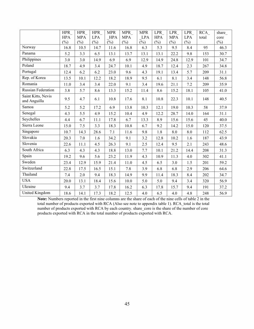
45

HPR_HPA (%)

HPR_MPA (%)

HPR_LPA (%)

MPR_HPA (%)

MPR_MPA (%)

MPR_LPA (%)

LPR_HPA (%)

LPR_MPA (%)

LPR_LPA (%)

RCA_ total

share_ core (%)

Norway 16.8 10.5 14.7 11.6 16.8 6.3 5.3 9.5 8.4 95 46.3 Panama 5.2 3.3 6.5 13.1 13.7 13.1 13.1 22.2 9.8 153 30.7 Philippines 3.0 3.0 14.9 6.9 6.9 12.9 14.9 24.8 12.9 101 34.7 Poland 18.7 4.9 3.4 24.7 10.1 4.9 18.7 12.4 2.3 267 34.8 Portugal 12.4 6.2 6.2 23.0 9.6 4.3 19.1 13.4 5.7 209 31.1 Rep. of Korea 13.5 10.1 12.2 18.2 18.9 9.5 6.1 8.1 3.4 148 56.8 Romania 11.0 3.4 3.4 22.0 9.1 3.4 19.6 21.1 7.2 209 35.9 Russian Federation 3.8 5.7 8.6 13.3 15.2 11.4 8.6 15.2 18.1 105 41.0 Saint Kitts, Nevis and Anguilla 9.5 4.7 6.1 10.8 17.6 8.1 10.8 22.3 10.1 148 40.5

Samoa 5.2 5.2 17.2 6.9 13.8 10.3 12.1 19.0 10.3 58 37.9 Senegal 4.3 5.5 4.9 15.2 10.4 4.9 12.2 28.7 14.0 164 31.1 Seychelles 4.4 6.7 11.1 17.8 6.7 13.3 8.9 15.6 15.6 45 40.0 Sierra Leone 15.0 7.5 3.3 18.3 10.8 6.7 9.2 14.2 15.0 120 37.5 Singapore 10.7 14.3 28.6 7.1 11.6 9.8 1.8 8.0 8.0 112 62.5 Slovakia 20.3 7.0 1.6 34.2 9.1 3.2 12.8 10.2 1.6 187 43.9 Slovenia 22.6 11.1 4.5 26.3 9.1 2.5 12.4 9.5 2.1 243 48.6 South Africa 6.3 4.3 4.3 18.8 13.0 7.7 10.1 21.2 14.4 208 31.3 Spain 19.2 9.6 5.6 23.2 11.9 4.3 10.9 11.3 4.0 302 41.1 Sweden 23.4 12.9 15.9 21.4 11.0 4.5 6.5 3.0 1.5 201 59.2 Switzerland 22.8 17.5 16.5 15.1 7.8 3.9 6.8 6.8 2.9 206 64.6 Thailand 7.4 2.0 9.4 18.3 14.9 9.9 11.4 18.3 8.4 202 34.7 USA 20.0 13.1 18.4 15.6 10.0 5.0 5.0 9.4 3.4 320 56.9 Ukraine 9.4 3.7 3.7 17.8 16.2 6.3 17.8 15.7 9.4 191 37.2 United Kingdom 18.6 14.1 17.3 18.2 12.5 4.0 6.5 4.0 4.8 248 56.9

Note: Numbers reported in the first nine columns are the share of each of the nine cells of table 2 in the total number of products exported with RCA (Also see note to appendix table 1). RCA_total is the total number of products exported with RCA by each country. share_core is the share of the number of core products exported with RCA in the total number of products exported with RCA.

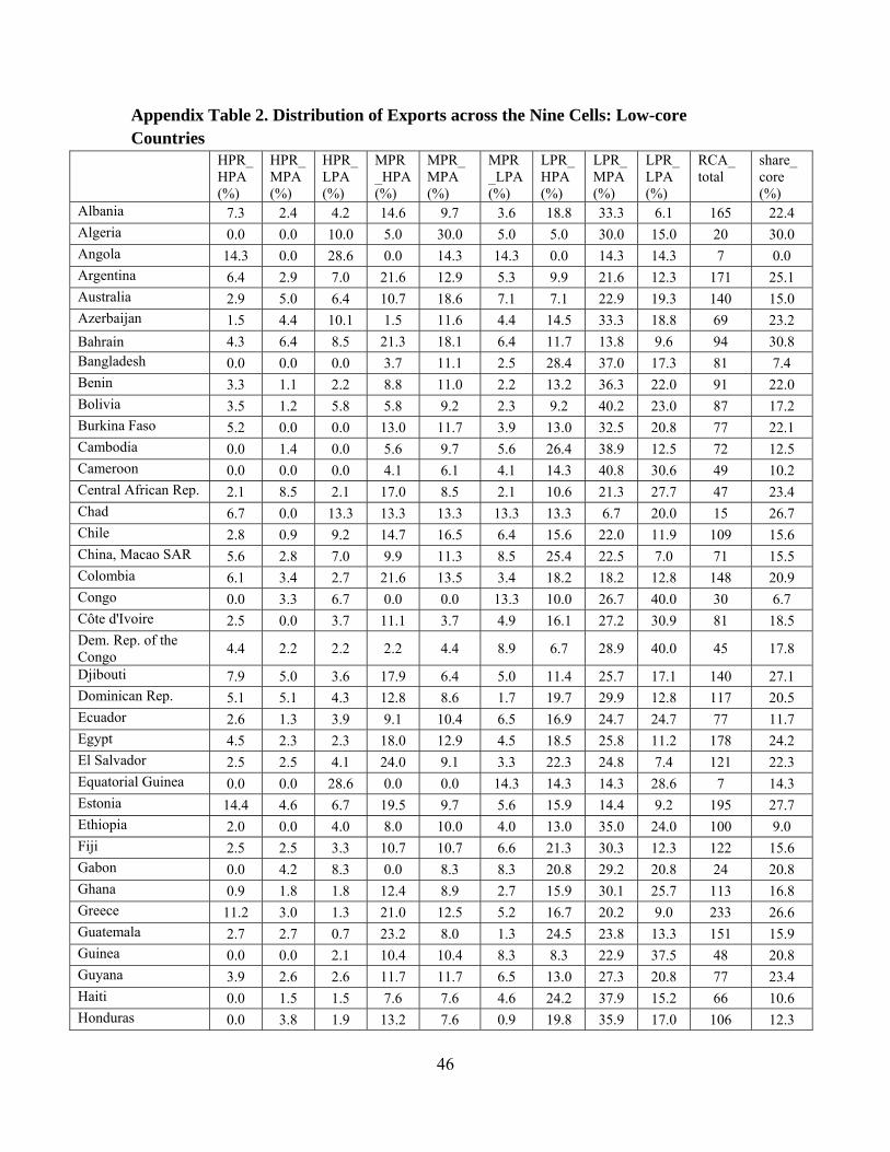
46

Appendix Table 2. Distribution of Exports across the Nine Cells: Low-core Countries

HPR_HPA (%)

HPR_MPA (%)

HPR_LPA (%)

MPR_HPA (%)

MPR_MPA (%)

MPR_LPA (%)

LPR_HPA (%)

LPR_MPA (%)

LPR_LPA (%)

RCA_ total

share_ core (%)

Albania 7.3 2.4 4.2 14.6 9.7 3.6 18.8 33.3 6.1 165 22.4 Algeria 0.0 0.0 10.0 5.0 30.0 5.0 5.0 30.0 15.0 20 30.0 Angola 14.3 0.0 28.6 0.0 14.3 14.3 0.0 14.3 14.3 7 0.0 Argentina 6.4 2.9 7.0 21.6 12.9 5.3 9.9 21.6 12.3 171 25.1 Australia 2.9 5.0 6.4 10.7 18.6 7.1 7.1 22.9 19.3 140 15.0 Azerbaijan 1.5 4.4 10.1 1.5 11.6 4.4 14.5 33.3 18.8 69 23.2 Bahrain 4.3 6.4 8.5 21.3 18.1 6.4 11.7 13.8 9.6 94 30.8 Bangladesh 0.0 0.0 0.0 3.7 11.1 2.5 28.4 37.0 17.3 81 7.4 Benin 3.3 1.1 2.2 8.8 11.0 2.2 13.2 36.3 22.0 91 22.0 Bolivia 3.5 1.2 5.8 5.8 9.2 2.3 9.2 40.2 23.0 87 17.2 Burkina Faso 5.2 0.0 0.0 13.0 11.7 3.9 13.0 32.5 20.8 77 22.1 Cambodia 0.0 1.4 0.0 5.6 9.7 5.6 26.4 38.9 12.5 72 12.5 Cameroon 0.0 0.0 0.0 4.1 6.1 4.1 14.3 40.8 30.6 49 10.2 Central African Rep. 2.1 8.5 2.1 17.0 8.5 2.1 10.6 21.3 27.7 47 23.4 Chad 6.7 0.0 13.3 13.3 13.3 13.3 13.3 6.7 20.0 15 26.7 Chile 2.8 0.9 9.2 14.7 16.5 6.4 15.6 22.0 11.9 109 15.6 China, Macao SAR 5.6 2.8 7.0 9.9 11.3 8.5 25.4 22.5 7.0 71 15.5 Colombia 6.1 3.4 2.7 21.6 13.5 3.4 18.2 18.2 12.8 148 20.9 Congo 0.0 3.3 6.7 0.0 0.0 13.3 10.0 26.7 40.0 30 6.7 Côte d'Ivoire 2.5 0.0 3.7 11.1 3.7 4.9 16.1 27.2 30.9 81 18.5 Dem. Rep. of the Congo 4.4 2.2 2.2 2.2 4.4 8.9 6.7 28.9 40.0 45 17.8

Djibouti 7.9 5.0 3.6 17.9 6.4 5.0 11.4 25.7 17.1 140 27.1 Dominican Rep. 5.1 5.1 4.3 12.8 8.6 1.7 19.7 29.9 12.8 117 20.5 Ecuador 2.6 1.3 3.9 9.1 10.4 6.5 16.9 24.7 24.7 77 11.7 Egypt 4.5 2.3 2.3 18.0 12.9 4.5 18.5 25.8 11.2 178 24.2 El Salvador 2.5 2.5 4.1 24.0 9.1 3.3 22.3 24.8 7.4 121 22.3 Equatorial Guinea 0.0 0.0 28.6 0.0 0.0 14.3 14.3 14.3 28.6 7 14.3 Estonia 14.4 4.6 6.7 19.5 9.7 5.6 15.9 14.4 9.2 195 27.7 Ethiopia 2.0 0.0 4.0 8.0 10.0 4.0 13.0 35.0 24.0 100 9.0 Fiji 2.5 2.5 3.3 10.7 10.7 6.6 21.3 30.3 12.3 122 15.6 Gabon 0.0 4.2 8.3 0.0 8.3 8.3 20.8 29.2 20.8 24 20.8 Ghana 0.9 1.8 1.8 12.4 8.9 2.7 15.9 30.1 25.7 113 16.8 Greece 11.2 3.0 1.3 21.0 12.5 5.2 16.7 20.2 9.0 233 26.6 Guatemala 2.7 2.7 0.7 23.2 8.0 1.3 24.5 23.8 13.3 151 15.9 Guinea 0.0 0.0 2.1 10.4 10.4 8.3 8.3 22.9 37.5 48 20.8 Guyana 3.9 2.6 2.6 11.7 11.7 6.5 13.0 27.3 20.8 77 23.4 Haiti 0.0 1.5 1.5 7.6 7.6 4.6 24.2 37.9 15.2 66 10.6 Honduras 0.0 3.8 1.9 13.2 7.6 0.9 19.8 35.9 17.0 106 12.3

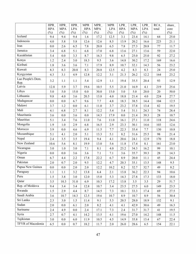
47

HPR_HPA (%)

HPR_MPA (%)

HPR_LPA (%)

MPR_HPA (%)

MPR_MPA (%)

MPR_LPA (%)

LPR_HPA (%)

LPR_MPA (%)

LPR_LPA (%)

RCA_ total

share_ core (%)

Iceland 9.4 9.4 9.4 1.6 17.2 12.5 3.1 23.4 14.1 64 25.0 Indonesia 4.0 5.8 5.8 12.6 12.6 8.5 13.9 20.2 16.6 223 21.1 Iran 0.0 2.6 6.5 7.8 20.8 6.5 7.8 27.3 20.8 77 11.7 Jamaica 3.4 6.8 5.1 6.8 17.0 6.8 13.6 27.1 13.6 59 22.0 Kazakhstan 5.4 0.0 3.3 8.7 16.3 9.8 6.5 25.0 25.0 92 27.2 Kenya 1.2 2.4 3.0 18.3 9.5 3.6 14.8 30.2 17.2 169 16.6 Kiribati 1.8 3.6 3.6 7.1 17.9 8.9 10.7 32.1 14.3 56 23.2 Kuwait 8.3 8.3 20.8 8.3 20.8 12.5 4.2 8.3 8.3 24 25.0 Kyrgyzstan 4.3 3.1 4.9 12.8 12.2 3.1 21.3 26.2 12.2 164 23.2 Lao People's Dem. Rep. 3.2 1.1 1.1 5.4 12.9 1.1 19.4 35.5 20.4 93 12.9

Latvia 12.8 5.9 3.7 19.6 10.5 5.5 21.0 16.9 4.1 219 25.6 Libya 5.0 5.0 15.0 0.0 30.0 15.0 5.0 5.0 20.0 20 50.0 Lithuania 9.8 4.0 3.6 20.5 13.8 4.0 18.8 21.4 4.0 224 27.7 Madagascar 0.0 0.0 6.7 9.6 7.7 4.8 18.3 38.5 14.4 104 12.5 Malawi 3.7 1.2 0.0 6.1 11.0 3.7 23.2 37.8 13.4 82 19.5 Mali 4.1 6.8 2.7 8.1 12.2 5.4 5.4 31.1 24.3 74 28.4 Mauritania 3.6 0.0 3.6 0.0 14.3 17.9 0.0 21.4 39.3 28 10.7 Mauritius 5.1 3.4 7.6 11.0 7.6 11.0 16.1 27.1 11.0 118 24.6 Mongolia 1.9 1.0 2.9 6.8 16.5 2.9 23.3 30.1 14.6 103 12.6 Morocco 3.9 0.0 4.6 6.9 11.5 7.7 22.3 35.4 7.7 130 10.8 Mozambique 5.1 4.1 2.0 5.1 13.3 5.1 8.2 31.6 25.5 98 21.4 Nepal 2.4 3.5 3.5 19.4 9.4 4.1 20.6 24.1 12.9 170 18.8 New Zealand 10.6 5.6 8.1 19.9 13.0 5.6 11.8 17.4 8.1 161 23.0 Nicaragua 3.0 1.0 3.0 7.1 8.1 4.0 23.2 34.3 16.2 99 10.1 Nigeria 0.0 0.0 3.6 3.6 7.1 7.1 3.6 35.7 39.3 28 14.3 Oman 6.7 4.4 2.2 17.8 22.2 6.7 8.9 20.0 11.1 45 24.4 Pakistan 2.0 0.7 2.0 9.5 12.2 4.7 20.3 35.1 13.5 148 9.5 Papua New Guinea 0.0 0.0 2.0 2.0 12.2 10.2 8.2 32.7 32.7 49 8.2 Paraguay 1.1 1.1 3.2 13.8 6.4 2.1 13.8 36.2 22.3 94 10.6 Peru 1.5 3.8 3.0 12.0 15.0 5.3 14.3 27.8 17.3 133 18.0 Qatar 3.5 10.3 31.0 6.9 10.3 17.2 13.8 3.5 3.5 29 51.7 Rep. of Moldova 9.4 3.4 3.4 12.8 10.7 3.4 23.5 27.5 6.0 149 23.5 Rwanda 1.5 2.9 4.4 8.7 14.5 7.3 10.1 33.3 17.4 69 27.5 Saudi Arabia 3.6 10.7 14.3 12.5 19.6 10.7 8.9 10.7 8.9 56 30.4 Sri Lanka 2.3 3.0 1.5 11.4 9.1 5.3 20.5 28.0 18.9 132 9.1 Sudan 2.0 0.0 6.1 2.0 8.2 4.1 4.1 42.9 30.6 49 16.3 Suriname 2.4 4.9 0.0 2.4 17.1 7.3 2.4 31.7 31.7 41 19.5 Syria 2.7 0.7 4.1 14.2 13.5 4.1 19.6 27.0 14.2 148 11.5 Tajikistan 3.0 0.0 6.0 11.9 10.5 4.5 14.9 35.8 13.4 67 22.4 TFYR of Macedonia 6.5 0.0 0.7 18.2 11.7 2.0 26.0 28.6 6.5 154 22.1

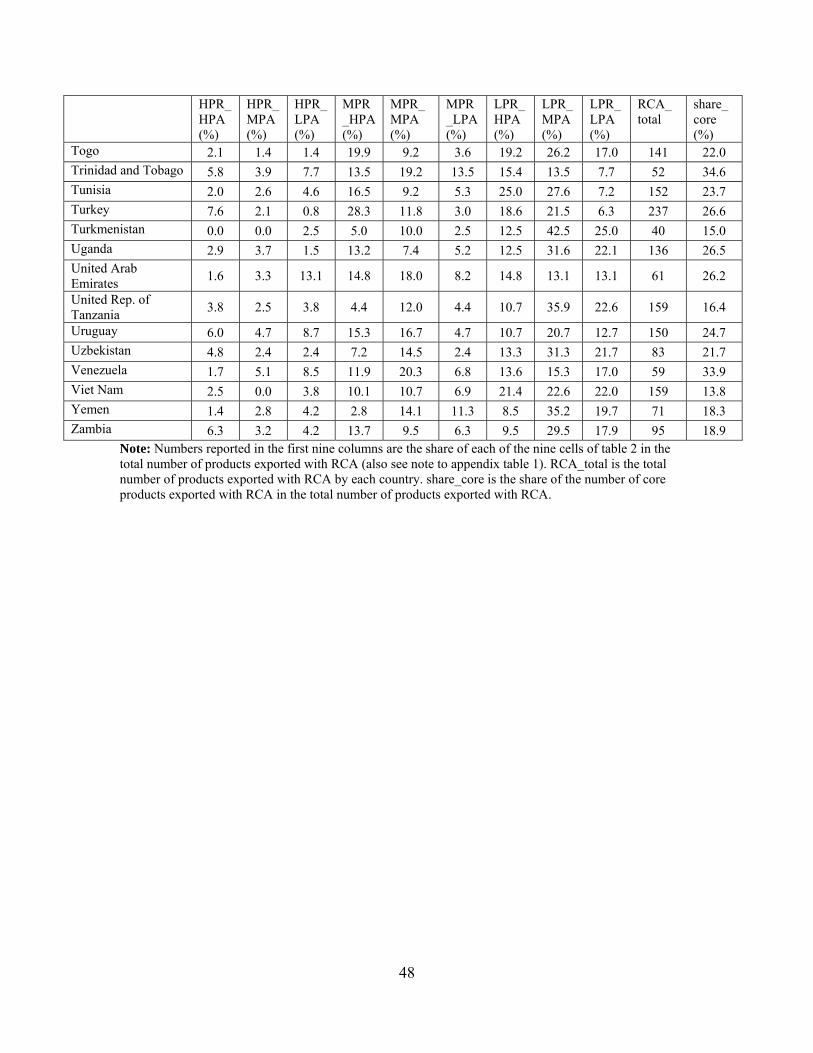
48

HPR_HPA (%)

HPR_MPA (%)

HPR_LPA (%)

MPR_HPA (%)

MPR_MPA (%)

MPR_LPA (%)

LPR_HPA (%)

LPR_MPA (%)

LPR_LPA (%)

RCA_ total

share_ core (%)

Togo 2.1 1.4 1.4 19.9 9.2 3.6 19.2 26.2 17.0 141 22.0 Trinidad and Tobago 5.8 3.9 7.7 13.5 19.2 13.5 15.4 13.5 7.7 52 34.6 Tunisia 2.0 2.6 4.6 16.5 9.2 5.3 25.0 27.6 7.2 152 23.7 Turkey 7.6 2.1 0.8 28.3 11.8 3.0 18.6 21.5 6.3 237 26.6 Turkmenistan 0.0 0.0 2.5 5.0 10.0 2.5 12.5 42.5 25.0 40 15.0 Uganda 2.9 3.7 1.5 13.2 7.4 5.2 12.5 31.6 22.1 136 26.5 United Arab Emirates 1.6 3.3 13.1 14.8 18.0 8.2 14.8 13.1 13.1 61 26.2

United Rep. of Tanzania 3.8 2.5 3.8 4.4 12.0 4.4 10.7 35.9 22.6 159 16.4

Uruguay 6.0 4.7 8.7 15.3 16.7 4.7 10.7 20.7 12.7 150 24.7 Uzbekistan 4.8 2.4 2.4 7.2 14.5 2.4 13.3 31.3 21.7 83 21.7 Venezuela 1.7 5.1 8.5 11.9 20.3 6.8 13.6 15.3 17.0 59 33.9 Viet Nam 2.5 0.0 3.8 10.1 10.7 6.9 21.4 22.6 22.0 159 13.8 Yemen 1.4 2.8 4.2 2.8 14.1 11.3 8.5 35.2 19.7 71 18.3 Zambia 6.3 3.2 4.2 13.7 9.5 6.3 9.5 29.5 17.9 95 18.9

Note: Numbers reported in the first nine columns are the share of each of the nine cells of table 2 in the total number of products exported with RCA (also see note to appendix table 1). RCA_total is the total number of products exported with RCA by each country. share_core is the share of the number of core products exported with RCA in the total number of products exported with RCA.

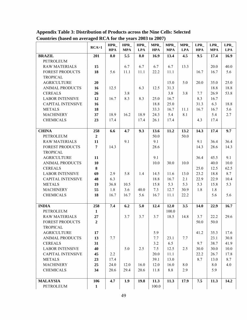
49

Appendix Table 3: Distribution of Products across the Nine Cells: Selected Countries (based on averaged RCA for the years 2003 to 2007)

RCA>1

HPR_HPA

HPR_MPA

HPR_LPA

MPR_HPA

MPR_MPA

MPR_LPA

LPR_HPA

LPR_MPA

LPR_LPA

BRAZIL 201 8.0 5.5 8.0 16.9 13.4 4.5 9.5 17.4 16.9 PETROLEUM RAW MATERIALS 15 6.7 6.7 6.7 6.7 13.3 20.0 40.0 FOREST PRODUCTS 18 5.6 11.1 11.1 22.2 11.1 16.7 16.7 5.6

TROPICAL AGRICULTURE 20 15.0 5.0 20.0 35.0 25.0

ANIMAL PRODUCTS 16 12.5 6.3 12.5 31.3 18.8 18.8 CEREALS 26 3.8 3.8 3.8 7.7 26.9 53.8 LABOR INTENSIVE 12 16.7 8.3 8.3 25.0 16.7 8.3 16.7 CAPITAL INTENSIVE 16 18.8 25.0 31.3 6.3 18.8 METALS 18 33.3 16.7 11.1 16.7 16.7 5.6 MACHINERY 37 18.9 16.2 18.9 24.3 5.4 8.1 5.4 2.7 CHEMICALS 23 17.4 17.4 26.1 17.4 4.3 17.4 CHINA 258 6.6 4.7 9.3 13.6 11.2 13.2 14.3 17.4 9.7 PETROLEUM 2 50.0 50.0 RAW MATERIALS 11 9.1 9.1 9.1 36.4 36.4 FOREST PRODUCTS 7 14.3 28.6 14.3 28.6 14.3

TROPICAL AGRICULTURE 11 9.1 36.4 45.5 9.1

ANIMAL PRODUCTS 10 10.0 30.0 10.0 40.0 10.0 CEREALS 8 25.0 12.5 62.5 LABOR INTENSIVE 69 2.9 5.8 1.4 14.5 11.6 13.0 23.2 18.8 8.7 CAPITAL INTENSIVE 48 6.3 18.8 16.7 2.1 22.9 22.9 10.4 METALS 19 36.8 10.5 15.8 5.3 5.3 5.3 15.8 5.3 MACHINERY 55 1.8 3.6 40.0 7.3 12.7 30.9 1.8 1.8 CHEMICALS 18 16.7 16.7 5.6 16.7 11.1 22.2 5.6 5.6 INDIA 258 7.4 6.2 5.0 12.4 12.0 3.5 14.0 22.9 16.7 PETROLEUM 1 100.0 RAW MATERIALS 27 3.7 3.7 3.7 18.5 14.8 3.7 22.2 29.6 FOREST PRODUCTS 2 50.0 50.0

TROPICAL AGRICULTURE 17 5.9 41.2 35.3 17.6

ANIMAL PRODUCTS 13 7.7 7.7 23.1 7.7 23.1 30.8 CEREALS 31 3.2 6.5 9.7 38.7 41.9 LABOR INTENSIVE 40 5.0 2.5 7.5 12.5 2.5 30.0 30.0 10.0 CAPITAL INTENSIVE 45 2.2 20.0 11.1 22.2 26.7 17.8 METALS 23 17.4 39.1 13.0 8.7 13.0 8.7 MACHINERY 25 24.0 12.0 16.0 12.0 16.0 8.0 8.0 4.0 CHEMICALS 34 20.6 29.4 20.6 11.8 8.8 2.9 5.9 MALAYSIA 106 4.7 1.9 19.8 11.3 11.3 17.9 7.5 11.3 14.2 PETROLEUM 1 100.0

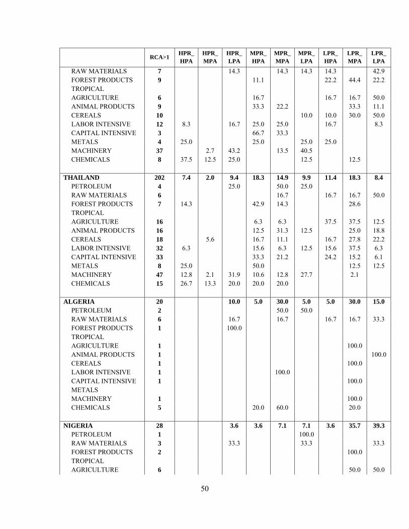
50

RCA>1

HPR_HPA

HPR_MPA

HPR_LPA

MPR_HPA

MPR_MPA

MPR_LPA

LPR_HPA

LPR_MPA

LPR_LPA

RAW MATERIALS 7 14.3 14.3 14.3 14.3 42.9 FOREST PRODUCTS 9 11.1 22.2 44.4 22.2

TROPICAL AGRICULTURE 6 16.7 16.7 16.7 50.0

ANIMAL PRODUCTS 9 33.3 22.2 33.3 11.1 CEREALS 10 10.0 10.0 30.0 50.0 LABOR INTENSIVE 12 8.3 16.7 25.0 25.0 16.7 8.3 CAPITAL INTENSIVE 3 66.7 33.3 METALS 4 25.0 25.0 25.0 25.0 MACHINERY 37 2.7 43.2 13.5 40.5 CHEMICALS 8 37.5 12.5 25.0 12.5 12.5 THAILAND 202 7.4 2.0 9.4 18.3 14.9 9.9 11.4 18.3 8.4 PETROLEUM 4 25.0 50.0 25.0 RAW MATERIALS 6 16.7 16.7 16.7 50.0 FOREST PRODUCTS 7 14.3 42.9 14.3 28.6

TROPICAL AGRICULTURE 16 6.3 6.3 37.5 37.5 12.5

ANIMAL PRODUCTS 16 12.5 31.3 12.5 25.0 18.8 CEREALS 18 5.6 16.7 11.1 16.7 27.8 22.2 LABOR INTENSIVE 32 6.3 15.6 6.3 12.5 15.6 37.5 6.3 CAPITAL INTENSIVE 33 33.3 21.2 24.2 15.2 6.1 METALS 8 25.0 50.0 12.5 12.5 MACHINERY 47 12.8 2.1 31.9 10.6 12.8 27.7 2.1 CHEMICALS 15 26.7 13.3 20.0 20.0 20.0 ALGERIA 20 10.0 5.0 30.0 5.0 5.0 30.0 15.0 PETROLEUM 2 50.0 50.0 RAW MATERIALS 6 16.7 16.7 16.7 16.7 33.3 FOREST PRODUCTS 1 100.0

TROPICAL AGRICULTURE 1 100.0

ANIMAL PRODUCTS 1 100.0 CEREALS 1 100.0 LABOR INTENSIVE 1 100.0 CAPITAL INTENSIVE 1 100.0 METALS MACHINERY 1 100.0 CHEMICALS 5 20.0 60.0 20.0 NIGERIA 28 3.6 3.6 7.1 7.1 3.6 35.7 39.3 PETROLEUM 1 100.0 RAW MATERIALS 3 33.3 33.3 33.3 FOREST PRODUCTS 2 100.0

TROPICAL AGRICULTURE 6 50.0 50.0

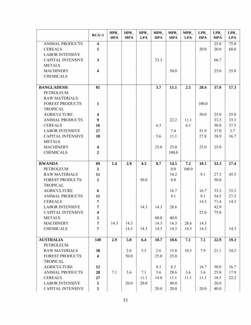
51

RCA>1

HPR_HPA

HPR_MPA

HPR_LPA

MPR_HPA

MPR_MPA

MPR_LPA

LPR_HPA

LPR_MPA

LPR_LPA

ANIMAL PRODUCTS 4 25.0 75.0 CEREALS 5 20.0 20.0 60.0 LABOR INTENSIVE CAPITAL INTENSIVE 3 33.3 66.7 METALS MACHINERY 4 50.0 25.0 25.0 CHEMICALS BANGLADESH 81 3.7 11.1 2.5 28.4 37.0 17.3 PETROLEUM RAW MATERIALS FOREST PRODUCTS 1 100.0

TROPICAL AGRICULTURE 4 50.0 25.0 25.0

ANIMAL PRODUCTS 9 22.2 11.1 33.3 33.3 CEREALS 16 6.3 6.3 50.0 37.5 LABOR INTENSIVE 27 7.4 51.9 37.0 3.7 CAPITAL INTENSIVE 18 5.6 11.1 27.8 38.9 16.7 METALS MACHINERY 4 25.0 25.0 25.0 25.0 CHEMICALS 2 100.0 RWANDA 69 1.4 2.9 4.3 8.7 14.5 7.2 10.1 33.3 17.4 PETROLEUM 2 0.0 100.0 RAW MATERIALS 11 18.2 9.1 27.3 45.5 FOREST PRODUCTS 2 50.0 0.0 50.0

TROPICAL AGRICULTURE 6 16.7 16.7 33.3 33.3

ANIMAL PRODUCTS 11 9.1 9.1 54.5 27.3 CEREALS 7 14.3 71.4 14.3 LABOR INTENSIVE 7 14.3 14.3 28.6 42.9 CAPITAL INTENSIVE 4 25.0 75.0 METALS 5 60.0 40.0 MACHINERY 7 14.3 14.3 14.3 14.3 28.6 14.3 CHEMICALS 7 14.3 14.3 14.3 14.3 14.3 14.3 14.3 AUSTRALIA 140 2.9 5.0 6.4 10.7 18.6 7.1 7.1 22.9 19.3 PETROLEUM RAW MATERIALS 38 2.6 5.3 2.6 15.8 10.5 7.9 21.1 34.2 FOREST PRODUCTS 4 50.0 25.0 25.0

TROPICAL AGRICULTURE 12 8.3 8.3 16.7 50.0 16.7

ANIMAL PRODUCTS 28 7.1 3.6 7.1 3.6 28.6 3.6 3.6 25.0 17.9 CEREALS 27 11.1 14.8 11.1 11.1 11.1 18.5 22.2 LABOR INTENSIVE 5 20.0 20.0 40.0 20.0 CAPITAL INTENSIVE 5 20.0 20.0 20.0 40.0

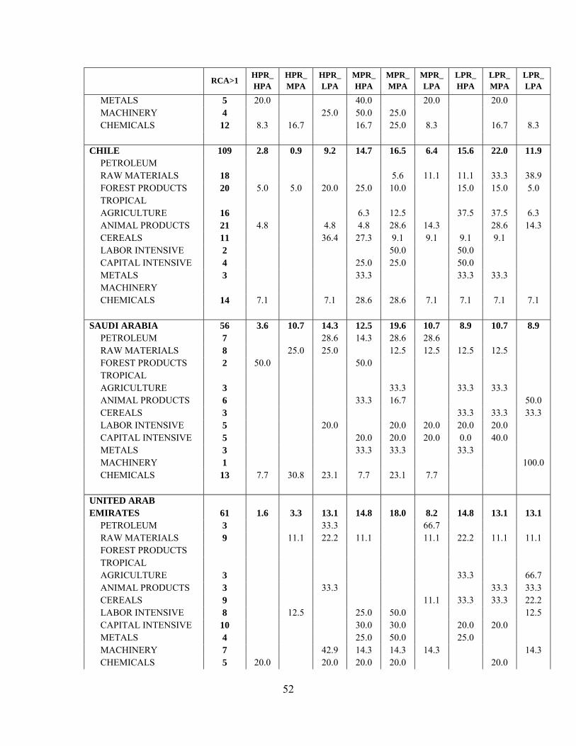
52

RCA>1

HPR_HPA

HPR_MPA

HPR_LPA

MPR_HPA

MPR_MPA

MPR_LPA

LPR_HPA

LPR_MPA

LPR_LPA

METALS 5 20.0 40.0 20.0 20.0 MACHINERY 4 25.0 50.0 25.0 CHEMICALS 12 8.3 16.7 16.7 25.0 8.3 16.7 8.3 CHILE 109 2.8 0.9 9.2 14.7 16.5 6.4 15.6 22.0 11.9 PETROLEUM RAW MATERIALS 18 5.6 11.1 11.1 33.3 38.9 FOREST PRODUCTS 20 5.0 5.0 20.0 25.0 10.0 15.0 15.0 5.0

TROPICAL AGRICULTURE 16 6.3 12.5 37.5 37.5 6.3

ANIMAL PRODUCTS 21 4.8 4.8 4.8 28.6 14.3 28.6 14.3 CEREALS 11 36.4 27.3 9.1 9.1 9.1 9.1 LABOR INTENSIVE 2 50.0 50.0 CAPITAL INTENSIVE 4 25.0 25.0 50.0 METALS 3 33.3 33.3 33.3 MACHINERY CHEMICALS 14 7.1 7.1 28.6 28.6 7.1 7.1 7.1 7.1 SAUDI ARABIA 56 3.6 10.7 14.3 12.5 19.6 10.7 8.9 10.7 8.9 PETROLEUM 7 28.6 14.3 28.6 28.6 RAW MATERIALS 8 25.0 25.0 12.5 12.5 12.5 12.5 FOREST PRODUCTS 2 50.0 50.0

TROPICAL AGRICULTURE 3 33.3 33.3 33.3

ANIMAL PRODUCTS 6 33.3 16.7 50.0 CEREALS 3 33.3 33.3 33.3 LABOR INTENSIVE 5 20.0 20.0 20.0 20.0 20.0 CAPITAL INTENSIVE 5 20.0 20.0 20.0 0.0 40.0 METALS 3 33.3 33.3 33.3 MACHINERY 1 100.0 CHEMICALS 13 7.7 30.8 23.1 7.7 23.1 7.7 UNITED ARAB EMIRATES 61 1.6 3.3 13.1 14.8 18.0 8.2 14.8 13.1 13.1 PETROLEUM 3 33.3 66.7 RAW MATERIALS 9 11.1 22.2 11.1 11.1 22.2 11.1 11.1 FOREST PRODUCTS

TROPICAL AGRICULTURE 3 33.3 66.7

ANIMAL PRODUCTS 3 33.3 33.3 33.3 CEREALS 9 11.1 33.3 33.3 22.2 LABOR INTENSIVE 8 12.5 25.0 50.0 12.5 CAPITAL INTENSIVE 10 30.0 30.0 20.0 20.0 METALS 4 25.0 50.0 25.0 MACHINERY 7 42.9 14.3 14.3 14.3 14.3 CHEMICALS 5 20.0 20.0 20.0 20.0 20.0

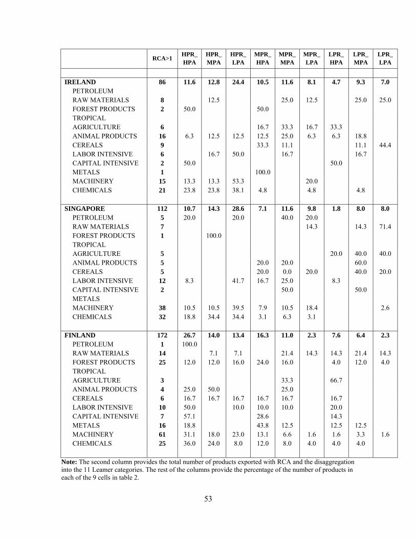
53

RCA>1

HPR_HPA

HPR_MPA

HPR_LPA

MPR_HPA

MPR_MPA

MPR_LPA

LPR_HPA

LPR_MPA

LPR_LPA

IRELAND 86 11.6 12.8 24.4 10.5 11.6 8.1 4.7 9.3 7.0 PETROLEUM RAW MATERIALS 8 12.5 25.0 12.5 25.0 25.0 FOREST PRODUCTS 2 50.0 50.0

TROPICAL AGRICULTURE 6 16.7 33.3 16.7 33.3

ANIMAL PRODUCTS 16 6.3 12.5 12.5 12.5 25.0 6.3 6.3 18.8 CEREALS 9 33.3 11.1 11.1 44.4 LABOR INTENSIVE 6 16.7 50.0 16.7 16.7 CAPITAL INTENSIVE 2 50.0 50.0 METALS 1 100.0 MACHINERY 15 13.3 13.3 53.3 20.0 CHEMICALS 21 23.8 23.8 38.1 4.8 4.8 4.8 SINGAPORE 112 10.7 14.3 28.6 7.1 11.6 9.8 1.8 8.0 8.0 PETROLEUM 5 20.0 20.0 40.0 20.0 RAW MATERIALS 7 14.3 14.3 71.4 FOREST PRODUCTS 1 100.0

TROPICAL AGRICULTURE 5 20.0 40.0 40.0

ANIMAL PRODUCTS 5 20.0 20.0 60.0 CEREALS 5 20.0 0.0 20.0 40.0 20.0 LABOR INTENSIVE 12 8.3 41.7 16.7 25.0 8.3 CAPITAL INTENSIVE 2 50.0 50.0 METALS MACHINERY 38 10.5 10.5 39.5 7.9 10.5 18.4 2.6 CHEMICALS 32 18.8 34.4 34.4 3.1 6.3 3.1 FINLAND 172 26.7 14.0 13.4 16.3 11.0 2.3 7.6 6.4 2.3 PETROLEUM 1 100.0 RAW MATERIALS 14 7.1 7.1 21.4 14.3 14.3 21.4 14.3 FOREST PRODUCTS 25 12.0 12.0 16.0 24.0 16.0 4.0 12.0 4.0

TROPICAL AGRICULTURE 3 33.3 66.7

ANIMAL PRODUCTS 4 25.0 50.0 25.0 CEREALS 6 16.7 16.7 16.7 16.7 16.7 16.7 LABOR INTENSIVE 10 50.0 10.0 10.0 10.0 20.0 CAPITAL INTENSIVE 7 57.1 28.6 14.3 METALS 16 18.8 43.8 12.5 12.5 12.5 MACHINERY 61 31.1 18.0 23.0 13.1 6.6 1.6 1.6 3.3 1.6 CHEMICALS 25 36.0 24.0 8.0 12.0 8.0 4.0 4.0 4.0

Note: The second column provides the total number of products exported with RCA and the disaggregation into the 11 Leamer categories. The rest of the columns provide the percentage of the number of products in each of the 9 cells in table 2.