How Smart Does an Agent Need to Be?

Scott Kirkpatrick1 and Johannes J. Schneider1,2

1Hebrew University of Jerusalem, Israeland

2Johannes Gutenberg University, Mainz, Germany

Abstract

The classic distributed computation is done by atoms, molecules, or spins in vastnumbers, each equipped with nothing more than knowledge of their immediateneighborhood and the rules of statistical mechanics. Such agents, 10^23 or more ofthem, are able to form liquids and solids from gases, realize extremely complex orderedstates, such as liquid crystals, and even decode encrypted messages. I'll describe a studydone for a sensor-array "challenge problem" in which we have based our approach onold-fashioned simulated annealing to accomplish target acquisition and tracking underthe rules of statistical mechanics. We believe the many additional constraints that occurin the real problem can be folded, step by step, into this stochastic approach. The resultshave applicability to other network management problems on scales where a distributedsolution will be mandatory.

Introduction

A very old idea in distributed computing and communication is the network that self-organizes to perform some local function of moderate complexity and thencommunicates its discoveries to some wider world that is interested. In militarycommunications, this might take the form of sensor arrays of simple, inexpensive units“sprinkled” behind a rapidly advancing force in battle to provide communications, oraround a sensitive installation to create a defensive perimeter. We recently participatedin a study of an application of this sort. From our experience, we concluded thatunderstanding the complexity of these self-organizing systems is critical to achievingtheir objectives, and is sorely neglected in the most popular approaches to programmingthem. The study which we joined (in midstream) had been envisioned as an exercise inmulti-agent distributed programming with negotiation protocols. These were to beemployed to resolve a difficult optimization problem, which would frequently requiresettling for locally sub-optimal results in order to meet challenging real time constraintswith acceptable solution quality.

The sensors in this array are Doppler radars, rather useless individually but capable oftracking targets if three or more of the radars can lock onto a single foreign object for asufficient time. In possible applications, such as protecting a aircraft carrier duringrefueling, one could imagine having a few thousand such antennas floating in the sea.But for research and demo purposes, controlling four to twenty such antennas wasconsidered quite challenging. Thus the temptation was strong to write very special-caseagents, and evolve very specific negotiation protocols as overloads and other problemswere discovered. One of the other groups in this study was planning to develop a target

1

selection protocol, with negotiation, that would support 64 antennas observing a dozenor so targets, and simulate it on a 32-processor server cluster, but not in real time.

Working with Bart Selman and the Intelligent Information Systems Institute of CornellUniversity, we were asked to determine if there might be phase transitions, or otherthreshold phenomena blocking the way to success in this endeavor, and if so, what to doabout it. We wrote a simulation of the target assignment and tracking problem.Because of our concern with complexity and its scaling, we treated the antennas asspins, not agents, and looked first for a Hamiltonian that would give them the rightbehavior, counting on statistical mechanics and temperature to handle the negotiationpart. It worked rather well, although there were a few inventions required to find a wayto make everything work. What follows is lightly edited from our progress reports.After describing our effort, we conclude with comments on the role of phase transitionsin this sort of large scale engineering problems as they continue to grow in scale overfuture decades.

Physics-inspired negotiation for Sensor Array self-organization

We implemented a family of models which borrow insights and techniques fromstatistical physics and use them to solve the sensor challenge problem under a series ofincreasing restrictive real-time constraints. We describe results with fairly difficultcommunications constraints and moving targets, covering the phases from targetacquisition to tracking. The method can deal with momentary overloads of targets bygracefully degrading coverage in the most congested areas, but picking up adequatecoverage as soon as the target density decreases in those areas, and holding it longenough for the target’s characteristics to be determined and a response initiated. Ourutility function-based approach could be extended to include more system-specificconstraints yet remained efficient enough to scale to larger numbers of sensors.

Our model consists of 100s of sensors attempting to track a number of targets. Thesensors are limited by their ability to communicate quickly and directly withneighboring sensors, and can see targets only over a finite range (which probablyexceeds the range over which they can communicate with one another). We take thecommunication limits to be approximately the values that arise in the Seabotdeployment by MITRE. This is modeled probabilistically. Initially we assumed thatthere is 90% probability of a communication link working between two neighboringsensors, 50% probability at twice that distance, and 10% probability at three times thatdistance, using a Fermi function for the calculation at an arbitrary distance.Subsequently, we explored other characteristic cutoff ranges for communications, usingthe same functional form for the probability of communication. At the start of eachsimulation we use this function to decide which communication links are working. Therange at which a target can be tracked is a parameter which we vary from a minimum of1.5 times a typical neighbor distance to 4 times this distance. Sensors are placed on aregular lattice, with positions varied from the lattice sites by a random displacement ofup to 0.1 times the lattice spacing. We considered three lattice arrangements to givedifferent spatial densities – honeycomb (sometimes called hexagonal) was the leastdense, then square lattice, then triangular lattice. But the precise lattice geometry madelittle difference beyond the changes in sensor density that resulted, so most work wascarried out with a square array of sensors, randomly displaced as described. Since three sensors must track a given target before an action decision can be taken, thismeans that at most 33 targets/100 sensors can be covered when no other constraints

2

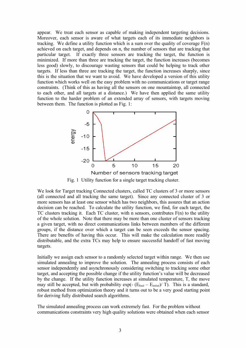
appear. We treat each sensor as capable of making independent targeting decisions.Moreover, each sensor is aware of what targets each of its immediate neighbors istracking. We define a utility function which is a sum over the quality of coverage F(n)achieved on each target, and depends on n, the number of sensors that are tracking thatparticular target. If exactly three sensors are tracking the target, the function isminimized. If more than three are tracking the target, the function increases (becomesless good) slowly, to discourage wasting sensors that could be helping to track othertargets. If less than three are tracking the target, the function increases sharply, sincethis is the situation that we want to avoid. We have developed a version of this utilityfunction which works well on the easy problem with no communications or target rangeconstraints. (Think of this as having all the sensors on one mountaintop, all connectedto each other, and all targets at a distance.) We have then applied the same utilityfunction to the harder problem of an extended array of sensors, with targets movingbetween them. The function is plotted as Fig. 1:

Fig. 1 Utility function for a single target tracking cluster.

We look for Target tracking Connected clusters, called TC clusters of 3 or more sensors(all connected and all tracking the same target). Since any connected cluster of 3 ormore sensors has at least one sensor which has two neighbors, this assures that an actiondecision can be reached. To calculate the utility function, we find, for each target, theTC clusters tracking it. Each TC cluster, with n sensors, contributes F(n) to the utilityof the whole solution. Note that there may be more than one cluster of sensors trackinga given target, with no direct communications links between members of the differentgroups, if the distance over which a target can be seen exceeds the sensor spacing.There are benefits of having this occur. This will make the calculation more readilydistributable, and the extra TCs may help to ensure successful handoff of fast movingtargets.

Initially we assign each sensor to a randomly selected target within range. We then usesimulated annealing to improve the solution. The annealing process consists of eachsensor independently and asynchronously considering switching to tracking some othertarget, and accepting the possible change if the utility function’s value will be decreasedby the change. If the utility function increases at simulated temperature, T, the movemay still be accepted, but with probability exp(- (Efinal – Einitial)/ T). This is a standard,robust method from optimization theory and it turns out to be a very good starting pointfor deriving fully distributed search algorithms.

The simulated annealing process can work extremely fast. For the problem withoutcommunications constraints very high quality solutions were obtained when each sensor

3

tried 1 to 3 target choices at each of only 3 temperatures. We have tuned our approachto the constrained problems to determine how robust this method will be at differentpoints in the “phase diagram” of sensor to target range, sensor communications rangeand delays. Our phase diagram parameters are:

• Average number of sensors communicating with a given sensor• Average number of sensors in range of an arbitrary target• Ratio of total number of targets to total number of sensors

We can use these normalized parameters to map out a phase diagram of feasiblesolutions (when the targets are uniformly distributed), and we use exact methods,limited to solving for very small numbers of sensors and targets, to identify the point atwhich a solution is 50% likely to be possible for a random, roughly uniformarrangement of targets. We then use our dynamic solution to treat a more difficult case– a swarm of targets arrive from outside the target array, then spread out, turningrandomly as they proceed. In this case we must deal at first with a load which is higherthan average, and targets which keep appearing from outside the boundaries of the array(to keep the total number constant as other targets exit). These results can be viewed intwo ways – impressionistically, as movies athttp://www.cs.huji.ac.il/~jsch/beautifulmovies/movies.html , or more quantitatively bymeasuring the actual length of time that each target is adequately covered by one ormore target connected clusters (TC clusters) in the sensor array. Each movie is actuallyan animated GIF file and rather large. When we first constructed these, each requiredabout 20 MB. Subsequently we found better encodings that reduced them to about 2MB each. They provide the raw material of our study. Finding good ways of analyzingthe performance of the whole system from the scenarios in the movies was one focus ofour research in this area. We developed arguments for using these overall performancemetrics as an assay for the rough location of the phase boundary to the region wheregood solutions could be found.

The conventions for the movies are as shown in the sample frame (Fig. 2) below. Eachsensor is identified by a blue cross. The sensors that are tracking a target and part of aTC show the antenna sector as a blue wedge. The targets are green dots, and eachtarget is surrounded with a green circle showing the range within which it can be sensed-- every sensor within that green circle can see the particular target if it chooses. Redlines connect sensors and targets tracked in a TC. The thermometer bar on the rightrepresents the fraction of targets covered by one or more TC’s. The wedgesrepresenting antenna sectors reflect a “real-world” issue that we inserted at this pointwithout actually modeling it as a constraint, and were later able to include within ouroptimization approach. Each of the prototype Doppler radars in the study had threeantenna cones, each cone capable of observing 120 degrees of azimuth. Only one conecould be active at a given time, and there were power and delay penalties for switchingthe sensor from one sector to another. We assumed that the sectors were oriented atrandom, with their angles fixed during the time that was simulated. This sort ofcomplication is extremely hard to add at late stages of an explicit programmingapproach, as would be typical of multiagent negotiation methods, but we were easilyable to explore it in our simulations.

4

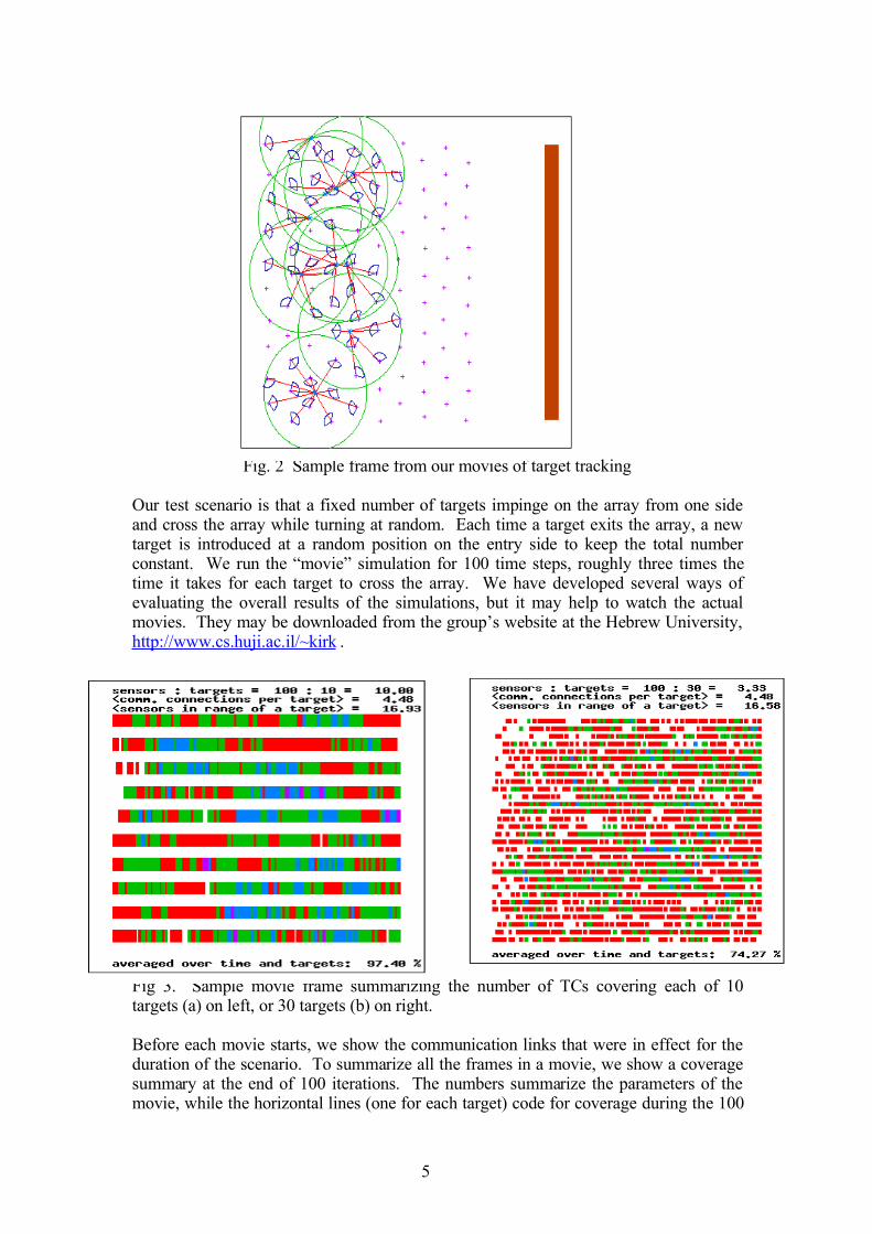
Fig. 2 Sample frame from our movies of target tracking

Our test scenario is that a fixed number of targets impinge on the array from one sideand cross the array while turning at random. Each time a target exits the array, a newtarget is introduced at a random position on the entry side to keep the total numberconstant. We run the “movie” simulation for 100 time steps, roughly three times thetime it takes for each target to cross the array. We have developed several ways ofevaluating the overall results of the simulations, but it may help to watch the actualmovies. They may be downloaded from the group’s website at the Hebrew University,http://www.cs.huji.ac.il/~kirk .

Fig 3. Sample movie frame summarizing the number of TCs covering each of 10targets (a) on left, or 30 targets (b) on right.

Before each movie starts, we show the communication links that were in effect for theduration of the scenario. To summarize all the frames in a movie, we show a coveragesummary at the end of 100 iterations. The numbers summarize the parameters of themovie, while the horizontal lines (one for each target) code for coverage during the 100

5

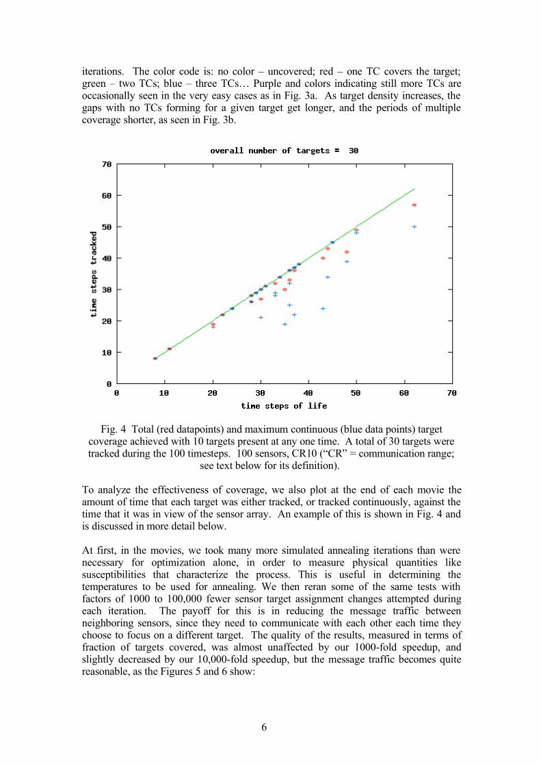
iterations. The color code is: no color – uncovered; red – one TC covers the target;green – two TCs; blue – three TCs… Purple and colors indicating still more TCs areoccasionally seen in the very easy cases as in Fig. 3a. As target density increases, thegaps with no TCs forming for a given target get longer, and the periods of multiplecoverage shorter, as seen in Fig. 3b.

Fig. 4 Total (red datapoints) and maximum continuous (blue data points) targetcoverage achieved with 10 targets present at any one time. A total of 30 targets weretracked during the 100 timesteps. 100 sensors, CR10 (“CR” = communication range;

see text below for its definition).

To analyze the effectiveness of coverage, we also plot at the end of each movie theamount of time that each target was either tracked, or tracked continuously, against thetime that it was in view of the sensor array. An example of this is shown in Fig. 4 andis discussed in more detail below.

At first, in the movies, we took many more simulated annealing iterations than werenecessary for optimization alone, in order to measure physical quantities likesusceptibilities that characterize the process. This is useful in determining thetemperatures to be used for annealing. We then reran some of the same tests withfactors of 1000 to 100,000 fewer sensor target assignment changes attempted duringeach iteration. The payoff for this is in reducing the message traffic betweenneighboring sensors, since they need to communicate with each other each time theychoose to focus on a different target. The quality of the results, measured in terms offraction of targets covered, was almost unaffected by our 1000-fold speedup, andslightly decreased by our 10,000-fold speedup, but the message traffic becomes quitereasonable, as the Figures 5 and 6 show:

6

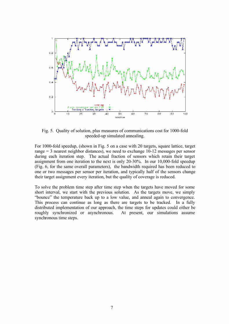
Fig. 5. Quality of solution, plus measures of communications cost for 1000-foldspeeded-up simulated annealing.

For 1000-fold speedup, (shown in Fig. 5 on a case with 20 targets, square lattice, targetrange = 3 nearest neighbor distances), we need to exchange 10-12 messages per sensorduring each iteration step. The actual fraction of sensors which retain their targetassignment from one iteration to the next is only 20-30%. In our 10,000-fold speedup(Fig. 6, for the same overall parameters), the bandwidth required has been reduced toone or two messages per sensor per iteration, and typically half of the sensors changetheir target assignment every iteration, but the quality of coverage is reduced.

To solve the problem time step after time step when the targets have moved for someshort interval, we start with the previous solution. As the targets move, we simply“bounce” the temperature back up to a low value, and anneal again to convergence.This process can continue as long as there are targets to be tracked. In a fullydistributed implementation of our approach, the time steps for updates could either beroughly synchronized or asynchronous. At present, our simulations assumesynchronous time steps.

7

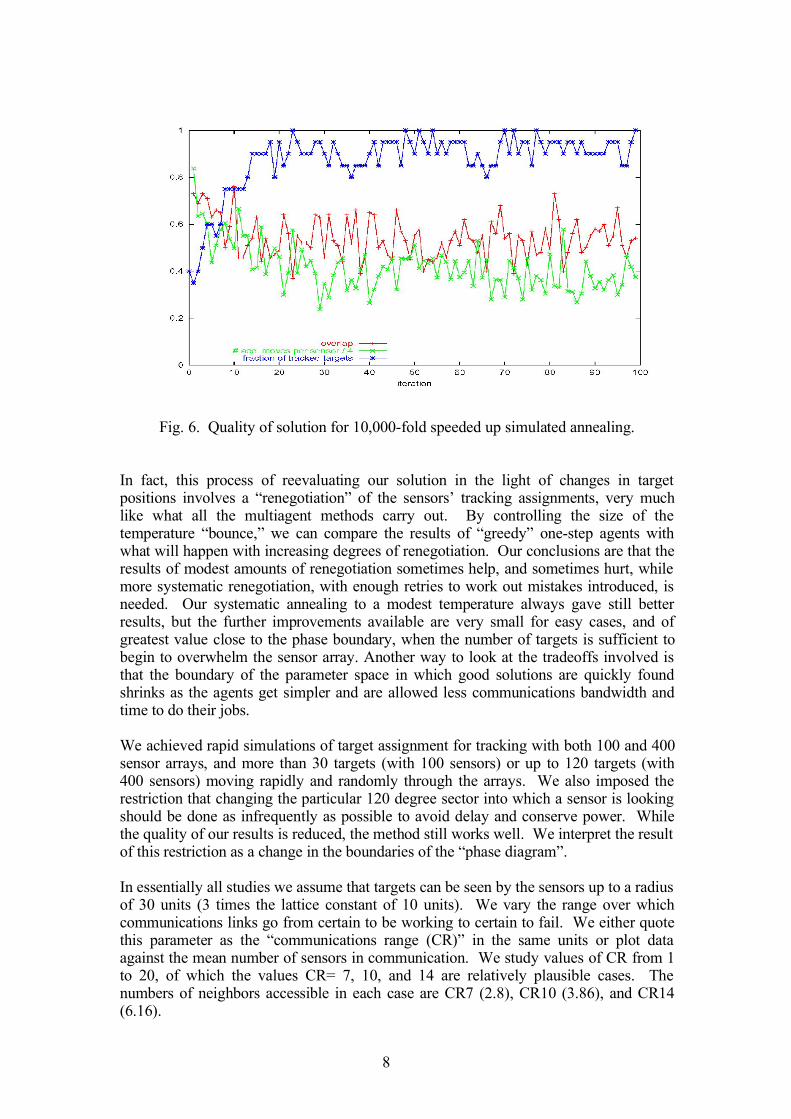
Fig. 6. Quality of solution for 10,000-fold speeded up simulated annealing.

In fact, this process of reevaluating our solution in the light of changes in targetpositions involves a “renegotiation” of the sensors’ tracking assignments, very muchlike what all the multiagent methods carry out. By controlling the size of thetemperature “bounce,” we can compare the results of “greedy” one-step agents withwhat will happen with increasing degrees of renegotiation. Our conclusions are that theresults of modest amounts of renegotiation sometimes help, and sometimes hurt, whilemore systematic renegotiation, with enough retries to work out mistakes introduced, isneeded. Our systematic annealing to a modest temperature always gave still betterresults, but the further improvements available are very small for easy cases, and ofgreatest value close to the phase boundary, when the number of targets is sufficient tobegin to overwhelm the sensor array. Another way to look at the tradeoffs involved isthat the boundary of the parameter space in which good solutions are quickly foundshrinks as the agents get simpler and are allowed less communications bandwidth andtime to do their jobs.

We achieved rapid simulations of target assignment for tracking with both 100 and 400sensor arrays, and more than 30 targets (with 100 sensors) or up to 120 targets (with400 sensors) moving rapidly and randomly through the arrays. We also imposed therestriction that changing the particular 120 degree sector into which a sensor is lookingshould be done as infrequently as possible to avoid delay and conserve power. Whilethe quality of our results is reduced, the method still works well. We interpret the resultof this restriction as a change in the boundaries of the “phase diagram”.

In essentially all studies we assume that targets can be seen by the sensors up to a radiusof 30 units (3 times the lattice constant of 10 units). We vary the range over whichcommunications links go from certain to be working to certain to fail. We either quotethis parameter as the “communications range (CR)” in the same units or plot dataagainst the mean number of sensors in communication. We study values of CR from 1to 20, of which the values CR= 7, 10, and 14 are relatively plausible cases. Thenumbers of neighbors accessible in each case are CR7 (2.8), CR10 (3.86), and CR14(6.16).

8

Finally, we explore the phase boundary for the physical modeling approach, with gentleannealing during each time step. We then compare these results with the results inwhich “renegotiation” during each time step is restricted or eliminated. We thenintroduce methods of controlling antenna sector usage more precisely, and give somemeasurements of the solution quality changes that result.

Phase boundary for target assignment:

The phase space of possible target swarm/sensor array combinations has at least threeparameters which we can study by considering sample scenarios in simulation. Theseare

• Average number of sensors that communicate with a direct single hop• Average number of sensors in range of an arbitrary target• Ratio of total number of targets to total number of sensors

We have considered the effect of target detection range, and concluded that as long astargets are detectable well outside the range of fast communications, the firstparameter, communications range, is the more critical. So in this report, we study theeffect of varying the ability to communicate from a situation where each sensor canreach only one or two neighbors in a single hop, to where a dozen or more neighborscan communicate directly.

The second summary figure (an example is shown in Fig. 4) after each movie is ascatter plot, for each of the targets that entered or crossed the sensor array, whichshows as a red data point the total number of time steps of successful tracking by thearray, and as a blue cross the longest consecutive string of time steps in which trackingwas achieved. The horizontal axis in this figure is the number of time steps that thetarget was within range of the array. When all the data points cluster close to thediagonal of this chart, we are successful in our tracking. Without an accepted model ofhow the sensors’ tracking information will be used, we do not know whether the totalfraction of the time for which a target has been accurately tracked or the time for whichtracking is continuous is more important. If we can afford the overhead of creating atarget agent to develop information about a particular target and to maintain its identityas it moves from one group of sensors to another, the total fraction of time the target isresolved is probably critical. If we want to use a simpler, more ad hoc architecture,continuous tracking may be critical. The fraction of time that a target is tracked,averaged over all targets that appear during a particular scenario, is the easiest singlemeasure of effectiveness to use in our analysis. For example, consider the loss ofsolution quality when running fewer iterations at each step in the annealing process(below). The average fraction falls only a little as we reduce the computing effort by afactor of 10^6 in an easy case (10 targets, 100 sensors, good communications). In amore difficult scenario (20 targets), the falloff of average coverage is faster at first, andthen accelerates at speedups beyond 1000 X. As a result of tests like that shown inFig. 7, we chose 100x as our standard speedup factor, to ensure reasonable results indifficult cases.

9

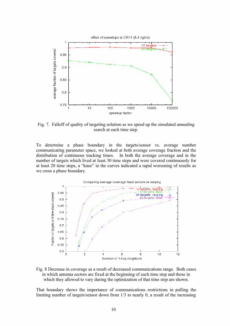
Fig. 7. Falloff of quality of targeting solution as we speed up the simulated annealingsearch at each time step.

To determine a phase boundary in the targets/sensor vs. average numbercommunicating parameter space, we looked at both average coverage fraction and thedistribution of continuous tracking times. In both the average coverage and in thenumber of targets which lived at least 30 time steps and were covered continuously forat least 20 time steps, a “knee” in the curves indicated a rapid worsening of results aswe cross a phase boundary.

Fig. 8 Decrease in coverage as a result of decreased communications range. Both casesin which antenna sectors are fixed at the beginning of each time step and those inwhich they allowed to vary during the optimization of that time step are shown.

That boundary shows the importance of communications restrictions in pulling thelimiting number of targets/sensor down from 1/3 to nearly 0, a result of the increasing

10

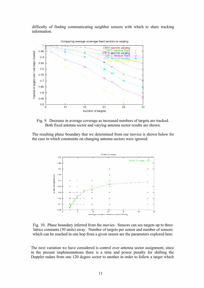
difficulty of finding communicating neighbor sensors with which to share trackinginformation.

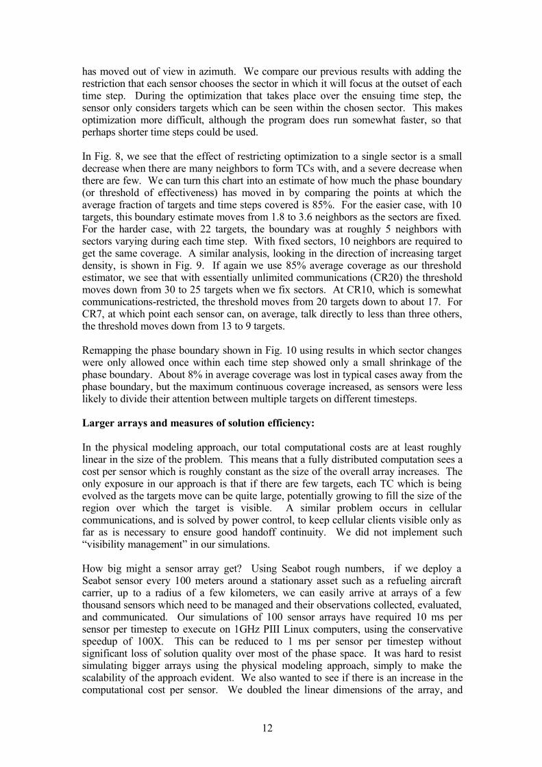
Fig. 9. Decrease in average coverage as increased numbers of targets are tracked.Both fixed antenna sector and varying antenna sector results are shown.

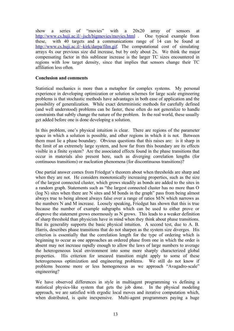
The resulting phase boundary that we determined from our movies is shown below forthe case in which constraints on changing antenna sectors were ignored:

Fig. 10. Phase boundary inferred from the movies. Sensors can see targets up to threelattice constants (30 units) away. Number of targets per sensor and number of sensorswhich can be reached in one hop from a given sensor are the parameters explored here.

The next variation we have considered is control over antenna sector assignment, sincein the present implementations there is a time and power penalty for shifting theDoppler radars from one 120 degree sector to another in order to follow a target which

11

has moved out of view in azimuth. We compare our previous results with adding therestriction that each sensor chooses the sector in which it will focus at the outset of eachtime step. During the optimization that takes place over the ensuing time step, thesensor only considers targets which can be seen within the chosen sector. This makesoptimization more difficult, although the program does run somewhat faster, so thatperhaps shorter time steps could be used.

In Fig. 8, we see that the effect of restricting optimization to a single sector is a smalldecrease when there are many neighbors to form TCs with, and a severe decrease whenthere are few. We can turn this chart into an estimate of how much the phase boundary(or threshold of effectiveness) has moved in by comparing the points at which theaverage fraction of targets and time steps covered is 85%. For the easier case, with 10targets, this boundary estimate moves from 1.8 to 3.6 neighbors as the sectors are fixed.For the harder case, with 22 targets, the boundary was at roughly 5 neighbors withsectors varying during each time step. With fixed sectors, 10 neighbors are required toget the same coverage. A similar analysis, looking in the direction of increasing targetdensity, is shown in Fig. 9. If again we use 85% average coverage as our thresholdestimator, we see that with essentially unlimited communications (CR20) the thresholdmoves down from 30 to 25 targets when we fix sectors. At CR10, which is somewhatcommunications-restricted, the threshold moves from 20 targets down to about 17. ForCR7, at which point each sensor can, on average, talk directly to less than three others,the threshold moves down from 13 to 9 targets.

Remapping the phase boundary shown in Fig. 10 using results in which sector changeswere only allowed once within each time step showed only a small shrinkage of thephase boundary. About 8% in average coverage was lost in typical cases away from thephase boundary, but the maximum continuous coverage increased, as sensors were lesslikely to divide their attention between multiple targets on different timesteps.

Larger arrays and measures of solution efficiency:

In the physical modeling approach, our total computational costs are at least roughlylinear in the size of the problem. This means that a fully distributed computation sees acost per sensor which is roughly constant as the size of the overall array increases. Theonly exposure in our approach is that if there are few targets, each TC which is beingevolved as the targets move can be quite large, potentially growing to fill the size of theregion over which the target is visible. A similar problem occurs in cellularcommunications, and is solved by power control, to keep cellular clients visible only asfar as is necessary to ensure good handoff continuity. We did not implement such“visibility management” in our simulations.

How big might a sensor array get? Using Seabot rough numbers, if we deploy aSeabot sensor every 100 meters around a stationary asset such as a refueling aircraftcarrier, up to a radius of a few kilometers, we can easily arrive at arrays of a fewthousand sensors which need to be managed and their observations collected, evaluated,and communicated. Our simulations of 100 sensor arrays have required 10 ms persensor per timestep to execute on 1GHz PIII Linux computers, using the conservativespeedup of 100X. This can be reduced to 1 ms per sensor per timestep withoutsignificant loss of solution quality over most of the phase space. It was hard to resistsimulating bigger arrays using the physical modeling approach, simply to make thescalability of the approach evident. We also wanted to see if there is an increase in thecomputational cost per sensor. We doubled the linear dimensions of the array, and

12

show a series of “movies” with a 20x20 array of sensors athttp://www.cs.huji.ac.il/~jsch/bigmovies/movies.html . One typical example fromthese, with 40 targets and a communications range of 14 can be found athttp://www.cs.huji.ac.il/~kirk/darpa/film.gif. The computational cost of simulatingarrays 4x our previous size did increase, but by only about 2x. We think the majorcompensating factor in this sublinear increase is the larger TC sizes encountered inregions with low target density, since that implies that sensors change their TCaffiliation less often.

Conclusion and comments

Statistical mechanics is more than a metaphor for complex systems. My personalexperience in developing optimization or solution schemes for large scale engineeringproblems is that stochastic methods have advantages in both ease of application and thepossibility of generalization. While exact deterministic methods for carefully defined(and well understood) problems can be faster, these often do not generalize to handleconstraints that subtly change the nature of the problem. In the real world, these usuallyget added before one is done developing a solution.

In this problem, one’s physical intuition is clear. There are regions of the parameterspace in which a solution is possible, and other regions in which it is not. Betweenthem must lie a phase boundary. Obvious questions that this raises are: is it sharp inthe limit of an extremely large system, and how far from this boundary are its effectsvisible in a finite system? Are the associated effects found in the phase transitions thatoccur in materials also present here, such as diverging correlation lengths (forcontinuous transitions) or nucleation phenomena (for discontinuous transitions)?

One partial answer comes from Friedgut’s theorem about when thresholds are sharp andwhen they are not. He considers monotonically increasing properties, such as the sizeof the largest connected cluster, which grows steadily as bonds are added to the sites ina random graph. Statements such as “the largest connected cluster has no more than O(log N) sites when there are N sites and M bonds in the graph” pass from being almostalways true to being almost always false over a range of ratios M/N which narrows asthe numbers N and M increase. Loosely speaking, Friedgut has shown that this is truebecause the number of example subgraphs which can be used to either prove ordisprove the statement grows enormously as N grows. This leads to a weaker definitionof sharp threshold than physicists have in mind when they think about phase transitions.But its generality supports the basic physical intuition. A second test, due to A. B.Harris, describes phase transitions that do not sharpen as the system size diverges. Hiscriterion is essentially that the correlation length for the type of ordering which isbeginning to occur as one approaches an ordered phase from one in which the order isabsent may not increase rapidly enough to allow the laws of large numbers to averagethe heterogeneous local environment into some more sharply characterized globalproperties. His criterion for smeared transition might apply to some of theseheterogeneous optimization and engineering problems. We still do not know ifproblems become more or less homogeneous as we approach “Avagadro-scale”engineering?

We have observed differences in style in multiagent programming vs defining astatistical physics-like system that gets the job done. In the physical modelingapproach, we are satisfied with ergodic local moves and iterative computation which,when distributed, is quite inexpensive. Multi-agent programmers paying a huge

13

constant factor in programming cost up front. They claim that they also scale due to theability to distribute the computation. However, multi-scale coordination occurs withoutexplicit effort in the statistical mechanics approach. Will it also be seen with staticallyprogrammed agents? I am skeptical, suspecting that the agents will have to invent acontrolling hierarchy as scale increases, and that this will have to be explicitlyprogrammed in or learned with awareness of their contexts.

References:

Simulated annealing science paperS. Kirkpatrick, C. D. Gelatt, Jr. and M. Vecchi, Science 200, 671 (1983).

Simulated annealing algorithms in Press’ bookW. H. Press, B. P. Flannery, S. A. Teukolsky, and W. T. Vetterling, “NumericalRecipes in C: The Art of Scientific Computing,” 2nd Edition, Canbridge Univ. Press(1993).

Bouncing and other non-monotonic annealing schedulesJ. Schneider, I. Morgenstern and J.M. Singer, Phys. Rev. E 58, 5085 (1998).P. N. Strenski and S. Kirkpatrick, Algorithmica 6, 346 (1991).

Stochastic Optimization -- Book in preparation by J. Schneider and S. Kirkpatrick(Springer 2004).

ANTS program proceedings DARPA e-book, Summer 2003.http://www.isi.edu/~szekeley/antsebook/ebook/

Friedgut’s theoremE. Friedgut, J. Am. Math. Soc. 12, 1017 (1999).

Harris criterion for smeared first order transitions A. B. Harris, J. Phys. C7, 1671 (1974).

14