how useful is bagging in forecasting economic time series ... kilian final version… · how useful...

How Useful is Bagging in Forecasting Economic Time

Series? A Case Study of U.S. CPI Inflation∗

Atsushi Inoue† Lutz Kilian‡

North Carolina State University University of Michigan

March 26, 2005

Abstract

This article explores the usefulness of bagging methods in forecasting economic time seriesfrom linear multiple regression models. We focus on the widely studied question of whetherthe inclusion of indicators of real economic activity lowers the prediction mean-squared error offorecast models of U.S. consumer price inflation. We study bagging methods for linear regressionmodels with correlated regressors and for factor models. We compare the accuracy of simulatedout-of-sample forecasts of inflation based on these bagging methods to that of alternative forecastmethods, including factor model forecasts, shrinkage estimator forecasts, combination forecastsand Bayesian model averaging. We find that bagging methods in this application are almost asacccurate or more accurate than the best alternatives. Our empirical analysis demonstrates thatlarge reductions in the prediction mean squared error are possible relative to existing methods, aresult that is also suggested by the asymptotic analysis of some stylized linear multiple regressionexamples.

KEYWORDS: Bootstrap aggregation; Bayesian model averaging; Forecast combination; Fac-tor models; Shrinkage estimation; Forecast model selection; Pre-testing.

∗We thank Bob Stine for stimulating our interest in bagging. We acknowledge helpful discussions with Todd Clark,Silvia Goncalves, Peter R. Hansen, Kirstin Hubrich, Mike McCracken, Massimiliano Marcellino, Serena Ng, BarbaraRossi, Jim Stock, Mark Watson, Jonathan Wright and Arnold Zellner. We thank seminar participants at Caltech,the CFS, the ECB, Johns Hopkins, Michigan State, Maryland, Purdue, and Tokyo. We have also benefited fromcomments received at the 2003 Triangle Econometrics Conference, the 2004 Financial Econometrics Conference inWaterloo, the 2004 Forecasting Conference at Duke, the 2004 North American Summer Econometric Society Meetingat Brown, the 2004 NBER-NSF Time Series Conference at SMU, the 2004 Midwest Econometrics Group Meeting atNorthwestern, and the 2004 CEPR Conference on Forecast Combinations in Brussels.

†Department of Agricultural and Resource Economics, Box 8109, North Carolina State University, Raleigh, NC27695-8109. E-mail: atsushi [email protected].

‡Department of Economics, University of Michigan, 611 Tappan Street, Ann Arbor, MI 48109-1220. E-mail:[email protected].

1 Introduction

A common problem in out-of-sample prediction is that the researcher suspects that many pre-dictors are potentially relevant, but few (if any) of these predictors individually are likely to havehigh predictive power. This problem is particularly relevant in economic forecasting, becauseeconomic theory rarely puts tight restrictions on the set of potential predictors. In addition,often alternative proxies of the same variable are available to the economic forecaster. A casein point are forecasts of consumer price inflation, which may involve a large number of alterna-tive measures of real economic activity such as the unemployment rate, industrial productiongrowth, housing starts, capacity utilization rates in manufacturing, or the number of help wantedpostings, to name a few.It is well known that forecasts generated using only one of these proxies tend to be unreliable

and unstable (see, e.g., Cecchetti, Chu and Steindel 2000, Stock and Watson 2003). On the otherhand, including all proxies (even if feasible) is thought to lead to overfitting and poor out-of-sample forecast accuracy. This fact suggests that we use formal statistical methods for selectingthe best subset of these predictors. Standard methods of comparing all possible combinationsof predictors by means of an information criterion function, however, become computationallyinfeasible when the number of potential predictors is moderately large.1

One strategy in this situation is to combine forecasts from many models with alternativesubsets of predictors. For example, one could use the mean, median or trimmed mean of theseforecasts as the final forecast or one could use regression-based weights for forecast combination(see Bates and Granger 1969, Stock and Watson 2003). There is no reason, however, for simpleaverages to be optimal, and the latter approach of regression-based weights tends to performpoorly in practice, unless some form of shrinkage estimation is used (see, e.g., Stock and Watson1999). More sophisticated methods of forecast model averaging weight individual forecasts bythe posterior probabilities of each forecast model (see, e.g., Min and Zellner 1993, Avramov 2002,Cremers 2002, Wright 2003a and Koop and Potter 2003 for applications in econometrics). ThisBayesian model averaging (BMA) approach has been used successfully in forecasting inflationby Wright (2003b). An alternative strategy involves shrinkage estimation of the unrestrictedmodel that includes all potentially relevant predictors. Such methods are routinely used forexample in the literature on Bayesian vector autoregressive models (see Litterman 1986). Athird strategy is to reduce the dimensionality of the regressor set by extracting the principalcomponents from the set of potential predictors. If the data are generated by an approximatefactor model, then factors estimated by principal components analysis can be used for efficientforecasting under quite general conditions (see, e.g., Stock and Watson 2002a, 2002b; Bai andNg 2004).2

A fourth strategy is to rely on a testing procedure for deciding which predictors to include inthe forecast model and which to drop. For example, we may fit a model including all potentially

1See Inoue and Kilian (2004) for a discussion of this and related approaches to ranking competing forecast models.The difficulty in using information criteria when the number of potential predictors, M , is large is that the criterionmust be evaluated for 2M combinations of predictors. For M > 20 this task tends to become computationallyprohibitive.

2A closely related approach to extracting common components has been developed by Forni et al. (2000, 2001)and applied in Forni et al. (2003).

1

relevant predictors, conduct a two-sided t-test for each predictor and discard all insignificantpredictors prior to forecasting. Such pre-tests lead to inherently unstable decision rules in thatsmall alterations in the data set may cause a predictor to be added or to be dropped. Thisinstability tends to inflate the variance of the forecasts and may undermine the accuracy of pre-test forecasts in applied work. The predictive accuracy of simple pre-test strategies, however,may be greatly enhanced by application of the bagging technique, leading to a fifth strategythat will be the focus of this paper.Bagging is a statistical method designed to reduce the out-of-sample prediction mean-squared

error of forecast models selected by unstable decision rules such as pre-tests. The term baggingis short for bootstrap aggregation (see Breiman 1996). In essence, bagging involves fitting theunrestricted model including all potential predictors to the original sample, generating a largenumber of bootstrap resamples from this approximation of the data, applying the pre-test ruleto each of the resamples, and averaging the forecasts from the models selected by the pre-teston each bootstrap sample.By averaging across resamples, bagging effectively removes the instability of the decision

rule. Hence, one would expect the variance of the bagged prediction model to be smaller thanthat of the model that would be selected based on the original data. Especially when thedecision rule is unstable, this variance reduction may be substantial. In contrast, the forecastbias of the prediction model is likely to be of similar magnitude, with or without bagging.This heuristic argument suggests that bagging will reduce the prediction mean squared errorof the regression model after variable selection. Indeed, there is substantial evidence of suchreductions in practice. There are some counterexamples, however, in which this intuition failsand bagging does not improve forecast accuracy. This fact has prompted increased interest inthe theoretical properties of bagging. Buhlmann and Yu (2002) recently have investigated theability of bagging to lower the asymptotic prediction mean-squared error (PMSE) of regressionswith a single regressor when the data are i.i.d. They show that bagging does not always improveon pre-testing, but nevertheless has the potential of achieving dramatic reductions in asymptoticforecast mean squared errors.In this article, we explore the usefulness of bagging methods in forecasting economic time

series from linear multiple regression models. Such forecasting models are routinely used bypractitioners, but no attempt has been made to utilize bagging methods in this context.3 Insection 2, we show how the bagging proposal may be adapted to applications involving mul-tiple regression models with possibly serially correlated and heteroskedastic errors. We brieflyreview the theory behind bagging, and - drawing on the analysis of the single-regressor modelin Buhlmann and Yu (2002) - provide some intuition for how and when bagging works in thesingle-regressor model with iid data. We then investigate the asymptotic properties of baggingin the multiple regressor model. We discuss applications of bagging in the correlated regressormodel as well as in factor models. Our analysis of some stylized examples shows that bagginghas the potential of reducing the asymptotic prediction mean-squared error in the multiple re-gressor model. This result holds when we apply the bagging method to theM largest estimatedfactors of a factor model, where M is treated as fixed, as well as when bagging is applied to

3In related work, Lee and Yang (2004) study the properties of bagging in binary prediction problems and quantileprediction of economic time series data.

2

the regressors of a correlated regressor model. In the latter case, the potential for asymptoticgains arises, whether the regressors have been orthogonalized or not, except when the degree ofcorrelation is very high.While these theoretical results are encouraging, they are not dispositive. First, the extent to

which the asymptotic gains in accuracy suggested by our theory translate into PMSE reductionsin finite samples is unclear. Second, our asymptotic analysis shows that the relative performanceof bagging will depend on unknown features of the data generating process, so the performanceof bagging must be assessed case by case. Third, our asymptotic results treat the regressors asexogenously given. This simplifying assumption facilitates the derivation of asymptotic results.When regressors are possibly endogenous, as seems plausible in many applications in economicsand finance, the asymptotic theory for the bagging predictor becomes intractable.4

We therefore recommend that, in practice, researchers choose between the alternative fore-casting methods based on the ranking of their recursive PMSEs in simulated out-of-sampleforecasts. In section 3, we illustrate this approach for a typical forecasting problem in eco-nomics. Specifically, we investigate whether one-month and twelve-month ahead CPI inflationforecasts for the United States may be improved upon by adding indicators of real economicactivity to models involving only lagged inflation rates. This empirical example is in the spirit ofrecent work by Stock and Watson (1999, 2003), Marcellino et al. (2003), Bernanke and Boivin(2003), Forni et al. (2003) and Wright (2003b), among others.We show that bagging is a very accurate forecasting procedure in this empirical application.

Bagging outperforms the benchmark model involving only lags of inflation, the unrestrictedmodel and factor models with rank 1, 2, 3, or 4 and different lag structures. Given thatbagging may be viewed as a shrinkage estimator, we also compare its performance to Bayesianshrinkage estimators. We find that bagging forecasts in some cases are almost as accurate as theforecast from the best Bayesian shrinkage estimator and in the others more accurate. Baggingalso is more accurate than forecast combination methods such as equal-weighted forecasts ofmodels including one indicator of real economic activity at a time or the type of BMA studiedby Wright (2003b). Finally, we show that bagging forecasts - depending on the horizon - arealmost as accurate as or somewhat more accurate than BMA forecasts generated using themethod of Raftery, Madigan and Hoeting (1997) that is based on randomly selected subsets ofthe predictors. The superior performance of bagging methods in this application is robust toincreasing the number of potential predictors by 25% and to decreasing it by 25%.We also contrast the relative performance of alternative methods of bagging in this context.

While all bagging methods perform well in this application, bagging predictors based on theorthogonalized regressors are slightly more accurate than those based on the untransformedregressors. Bagging predictors based on the M largest principal components also worked well.This finding is surprising as the cross-sectional dimension of our problem is relatively small,casting doubt on the applicability of standard asymptotic arguments for bagging factor models.An interesting avenue for future research will be the use of bagging methods on panels withlarge cross-sections that are commonly used in other forecasting applications. We conclude insection 4.

4A similar exogeneity assumption has also been used in the literature to facilitate the derivation of the PMSE offactor model forecasts (see, e.g., Bai and Ng 2004, p.4).

3

2 How Does Bagging Work?

Consider the forecasting model:

yt+h = β0xt + εt+h, h = 1, 2, 3, ... (1)

where εt+h denotes the h-step ahead linear forecast error, β is anM -dimensional column vectorof parameters and xt is a column vector of M predictors at time period t. We presume that ytand xt are stationary processes or have been suitably transformed to achieve stationarity.Let β denote the ordinary least-squares (OLS) estimator of β in (1) and let tj denote the

t-statistic for the null that βj is zero in the unrestricted model, where βj is the jth element ofβ. Further, let bγ denote the OLS estimator of the forecast model after variable selection. Notethat - unlike Buhlmann and Yu (2002) - we re-estimate the model after variable selection. Forxt ∈ <M , we define the predictor from the unrestricted model (UR), the predictor from thefully restricted model (FR), and the pre-test (PT ) predictor conditional on xT−h+1 by

yUR(xT−h+1) = β0xT−h+1,

yFR(xT−h+1) = 0,

yPT (xT−h+1) = 0, if |tj | < c ∀j and yPT (xT−h+1) = bγ0STxT−h+1 otherwise,where ST is the stochastic selection matrix obtained from the M ×M diagonal matrix with(i, i)th element I(|ti| > c) by deleting rows of zeros, and c is the critical value of the pre-test.The UR model forecast is based on the fitted values of a regression including allM potential

predictors. The FR model forecast emerges when all predictors are dropped, as in the well-known no-change forecast model of asset returns. The latter forecast sometimes is also referredto as a random walk forecast in the literature.The pre-test strategy that we analyze is particularly simple. We first fit the unrestricted

model that includes all potential predictors. We then conduct two-sided t-tests on each slopeparameter based on a pre-specified critical value c. We discard the insignificant predictorsand re-estimate the final model, before generating the PT forecast. In constructing the t-statistic we use appropriate standard errors that allow for serial correlation and/or conditionalheteroskedasticity. Specifically, when the error term follows an MA(h− 1) process, the pre-teststrategy may be implemented based on White (1980) robust standard errors for h = 1 or West(1997) robust standard errors for h > 1. For more general error structures, nonparametricrobust standard errors such as the HAC estimator proposed by Newey and West (1987) wouldbe appropriate.

2.1 Algorithm for Bagging Dynamic Regression Models

The bootstrap aggregated or bagging predictor is obtained by averaging the pre-test predictoracross bootstrap replications. Bagging can in principle be applied to any pre-testing strategy,not just to the specific pre-testing strategy discussed here, and there is no reason to believe thatour t-test strategy is optimal. Nevertheless, the simple t-test strategy studied here appears towork well in many cases.

4

Definition 1. [BA method] The bagging predictor in the standard regression framework is definedas follows:(i) Arrange the set of tuples (yt+h, x0t), t = 1, ..., T−h, in the form of a matrix of dimension

(T − h)× (M + 1):

y1+h x01...

...yT x0T−h

.

Construct bootstrap samples (y∗1+h, x0∗1 ), ..., (y

∗T , x

0∗T−h) by drawing with replacement blocks of

m rows of this matrix, where the block size m is chosen to capture the dependence in the errorterm (see, e.g., Hall and Horowitz 1996, Goncalves and White 2004).(ii) For each bootstrap sample, compute the bootstrap pre-test predictor conditional on xT−h+1

y∗PT (xT−h+1) = 0, if |t∗j | < c ∀j and y∗PT (xT−h+1) = bγ∗0S∗TxT−h+1 otherwise,where bγ∗and S∗T are the bootstrap analogues of bγand ST , respectively. In constructing |t∗j | we

compute the variance of√T bβ∗as bH∗−1 bV ∗ bH∗−1 where

bV ∗ =1

bm

bXk=1

mXi=1

mXj=1

(x∗(k−1)m+iε∗(k−1)m+i+h)(x

∗(k−1)m+jε

∗(k−1)m+j+h)

0,

bH∗ =1

bm

bXk=1

mXi=1

(x∗(k−1)m+ix∗0(k−1)m+i),

ε∗t+h = y∗t+h − bβ∗0x∗t , and b is the integer part of T/m (see, e.g., Inoue and Shintani 2003).(iii) The bagged predictor is the expectation of the bootstrap pre-test predictor across bootstrap

samples, conditional on xT−h+1:

yBA(xT−h+1) = E∗[bγ∗0S∗TxT−h+1],where E∗ denotes the expectation with respect to the bootstrap probability measure. The bootstrapexpectation in (iii) may be evaluated by simulation:

yBA(xT−h+1) =1

B

BXi=1

bγ∗i0S∗iT xT−h+1,

where B =∞ in theory. In practice, B = 100 tends to provide a reasonable approximation.

An important design parameter in applying bagging is the block size m. If the forecastmodel at horizon h is correctly specified in that E(εt+h|Ωt) = 0, where Ωt denotes the date t

5

information set, then m = h (see, e.g., Goncalves and Kilian 2004). Otherwise m > h. In thelatter case, data-dependent rules such as calibration may be used to determine m (see, e.g.,Politis, Romano and Wolf 1999).The performance of bagging will in general depend on the critical value chosen for pre-testing

not unlike the way in which shrinkage estimators depend on the degree of shrinkage. In practice,cmay be chosen by comparing the accuracy of the bagging forecast method for alternative valuesof c in simulated out-of-sample forecasts. This question will be taken up in section 3 when wediscuss the empirical application.

2.2 Asymptotic Properties of the Bagging Predictor in the Single-Regressor Model

Buhlmann and Yu (2002) have analyzed the asymptotic properties of the bagging algorithm inDefinition 1 for the special case of a linear model with only a single regressor when the dataare i.i.d. They showed that the BA predictor in many (but not all) cases has lower asymptoticPMSE than the PT predictor. It is instructive to review this evidence. Let β = δT−1/2, and,for expository purposes, suppose that xt = 1 ∀t, εt is distributed iid(0, σ2), σ2 = 1, and h = 1.In that case, the forecasts from the unrestricted (UR) model, the fully restricted (FR) modeland the pre-test (PT ) model, and the bagging (BA) forecast can be written as

yUR = β,

yFR = 0,

yPT = bβI(|T 1/2β| > c),

yBA =1

B

BXi=1

bβ∗iI(|T 1/2β∗i| > c).

We are interested in comparing the asymptotic PMSE of these predictors.

Definition 2. [APMSE] The asymptotic PMSE (or APMSE) is defined as the second-order termof the asymptotic approximation of the prediction mean squared error:

E[(y(x)− y(x))2] = σ2 +1

TAPMSE(y(x)) + o

µ1

T

¶.

Following Buhlmann and Yu (2002) it can be shown that:

APMSE(yUR(x)) = 1,

APMSE(yFR(x)) = δ2,

APMSE(yPT (x)) = E[(ξ − δ)I(|ξ| > c) + δI(|ξ| ≤ c)]2,

APMSE(yBA(x)) = E[δ − ξ + ξΦ(c− ξ)− φ(c− ξ)

−ξΦ(−c− ξ) + φ(−c− ξ)]2.

where ξ ∼ N(δ, 1).

6

How does the APMSE of the BA predictor compare to that of the PT predictor? Notethat the APMSE expression for the BA predictor does not depend on the indicator function,reflecting the smoothing implied by bootstrap aggregation. Although this smoothing shouldtypically help to reduce the forecast variance relative to the PT predictor, it is not obvious apriori whether bagging the pre-test predictor will also improve the APMSE. Figure 2 inves-tigates this question. We set c = 1.96 for expository purposes. The upper panel shows thesquared asymptotic bias of the two predictors. Although bagging does reduce the asymptoticbias somewhat for most values of δ, the gains are small. The second panel, in contrast, showsdramatic reductions in variance relative to the PT predictor for most δ, which, as shown inthe third panel, result in substantial improvements in the overall accuracy measured by theAPMSE. Figure 2 illustrates the potential of the bagging principle to improve forecast accu-racy relative to the pre-test. As noted by Buhlmann and Yu (2002), although this improvementdoes not occur for all values of δ, it does for a wide range of δ.More importantly, from our point of view, it can be shown that for some values of δ bagging

will have lower APMSE than the FR and UR predictors as well. We illustrate this fact inFigure 2, which plots the APMSEs of the UR, FR, PT and BA predictors as a function of δ.For δ > 1 the UR predictor has lower APMSE than the FR predictor, for δ = 1 both modelsare tied and for δ < 1 the FR predictor is asymptotically more accurate. Although the PTpredictor protects the user from choosing the UR forecast when δ is close to zero and the FRforecast when δ is large, the PT predictor for any given choice of δ is always dominated byeither the UR or the FR predictor.5 In contrast, the BA predictor not only dominates the PTpredictor for most values of δ, but for values of δ near one, it has the lowest APMSE of allpredictors shown in Figure 2.This stylized example based on Buhlmann and Yu (2002) conveys two valuable insights: First,

bagging under certain conditions can yield asymptotic improvements in the PMSE relative tothe UR, FR, and PT predictors. This fact suggests that it deserves further study. Second, theextent of these asymptotic improvements depends very much on unobservable features of thedata. Under some conditions bagging may actually result in a higher asymptotic PMSE thanalternative methods. This seems especially likely when the signal-to-noise ratio in the data isvery weak, as in forecasting asset returns for example. This is not a limitation of the baggingmethod alone, of course, but simply a reflection of the bias-variance trade-off in forecasting.The same type of problem would arise with any other forecasting method in the literature.

2.3 Asymptotic Properties of the Bagging Predictor in the Correlated-Regressor Model

The example of Buhlmann and Yu (2002), while instructive, is of limited relevance for applica-tions of bagging to the multiple linear regression model. In practice, predictors will inevitablybe correlated to various degrees and this correlation will affect the PMSE and potentially theranking of the forecasting methods. In this subsection, we will establish that the qualitativefindings of Buhlmann and Yu (2002) for the single-regressor model continue to hold in themultiple regressor model. We do so in the simplest possible setting when the regressors are iid.

5For a related discussion of the MSE of inequality constrained estimators see Thomson and Schmidt (1982).

7

2.3.1 Case 1: Bagging the Untransformed Predictors

We begin by deriving the APMSE for the UR, FR, PT , and BA predictors in the correlatedregressor model with iid regressors.

Assumption 1.

(a) xt and εt are iid over time with finite fourth moments and xt and εt are independent ofone another.

(b) yt = β0xt + εt where β = T−1/2δ.

(c) T−1/2PT

t=1 xtεtd→ N(0, σ2E(xtx

0t)) where σ

2 > 0 and E(xtx0t) is positive definite.

Proposition 1. Under Assumption 1

APMSE(yUR(x)) = E[(ξ − δ)0x]2,

APMSE(yFR(x)) = (δ0x)2,

APMSE(yPT (x)) = E[ξ0E(xtx0t)S

0(SE(xtx0t)S

0)−1SxI(∃j s.t. |ξj | > cqσ2[(E(xtx0t))

−1]jj)− δ0x]2,

APMSE(yBA(x)) = EE[ξ∗0E(xtx0t)S∗0(S∗E(xtx0t)S∗0)−1S∗xI(∃j s.t.|ξ∗j | > cqσ2[(E(xtx0t))

−1]jj)|ξ]− δ0x2

where ξ and ξ∗ are M -dimensional random vectors such that ξ ∼ N(δ, σ2[E(xtx0t)]−1) and

ξ∗|ξ ∼ N(ξ, σ2(E(xtx0t))−1), S is the stochastic selection matrix obtained from the M ×M

diagonal matrix with (i, i)th element I(|ξi| > cpσ2[(E(xtx0t))

−1]ii) by deleting rows of zeros,and S∗ is defined as S with ξ replaced by ξ∗.

The proof of Proposition 1 is in the Appendix.

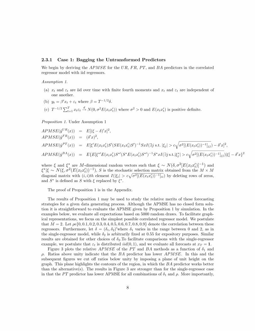
The results of Proposition 1 may be used to study the relative merits of these forecastingstrategies for a given data generating process. Although the APMSE has no closed form solu-tion it is straightforward to evaluate the APMSE given by Proposition 1 by simulation. In theexamples below, we evaluate all expectations based on 5000 random draws. To facilitate graph-ical representations, we focus on the simplest possible correlated regressor model. We postulatethatM = 2. Let ρ 0, 0.1, 0.2, 0.3, 0.4, 0.5, 0.6, 0.7, 0.8, 0.9 denote the correlation between theseregressors. Furthermore, let δ = (δ1, δ2)

0where δ1 varies in the range between 0 and 2, as inthe single-regressor model, while δ2 is arbitrarily fixed at 0.55 for expository purposes. Similarresults are obtained for other choices of δ2.To facilitate comparisons with the single-regressorexample, we postulate that εt is distributed iid(0, 1), and we evaluate all forecasts at xT = 1.Figure 3 plots the relative APMSE of the PT and BA methods as a function of δ1 and

ρ. Ratios above unity indicate that the BA predictor has lower APMSE. In this and thesubsequent figures we cut off ratios below unity by imposing a plane of unit height on thegraph. This plane highlights the contours of the region, in which the BA predictor works betterthan the alternative(s). The results in Figure 3 are stronger than for the single-regressor casein that the PT predictor has lower APMSE for all combinations of δ1 and ρ. More importantly,

8

Figure 4 establishes that there is a set of pairs of δ1 and ρ, for which the BA predictor haslower asymptotic PMSE than any of the other methods under consideration. As expected theBA predictor works best for intermediate ranges of δ1. When δ1 is very small or very large, theFR and UR predictors, respectively, will be more accurate than the BA predictor. The rangeof δ1, for which the BA predictor.has the lowest APMSE, shrinks somewhat, as ρ increases.The results in Figures 3 and 4 of course are specific to the stylized example. Here our aim

has only been to establish that there are potential asymptotic gains in accuracy from baggingeven in the correlated regressor model. How large these gains from bagging will be in practice,will depend on unknown features of the data generating process and is an empirical question.

2.3.2 Case 2: Bagging the Orthogonalized Predictors

One seeming drawback of the bagging proposal in Definition 1 is that when predictors arecorrelated the effective size of the t-tests on individual predictors will be distorted. This factsuggests an alternative approach to bagging in which the predictors are orthogonalized prior toconducting the t-tests. This may be accomplished as follows:

Definition 3. [CBA method] The bagging predictor for the orthogonalized regressors may beobtained via a Cholesky decomposition as follows:(i) Arrange the set of tuples (yt+h, x0t), t = 1, ..., T−h, in the form of a matrix of dimension

(T − h)× (M + 1):

y1+h x01...

...yT x0T−h

.

Construct bootstrap samples (y∗1+h, x0∗1 ), ..., (y

∗T , x

0∗T−h) by drawing with replacement blocks of

m rows of this matrix, where the block size m is chosen to capture the dependence in the errorterm.(ii) Compute the orthogonalized predictor ext = P 0−1xt, where P is the Cholesky decompo-

sition of E(xtx0t), i.e., the M ×M upper triangular matrix such that P 0P = E(xtx

0t). For each

bootstrap sample, compute the bootstrap pre-test predictor conditional on exT−h+1y∗PT (exT−h+1) = 0, if |t∗j | < c ∀j and y∗PT (exT−h+1) = bγ∗0S∗T exT−h+1 otherwise,

where bγ∗and S∗T are the bootstrap analogues of bγand ST , respectively, applied to the orthogo-

nalized predictor model. In constructing |t∗j | we compute the variance of√T bβ∗as bH∗−1 bV ∗ bH∗−1

where

9

bV ∗ =1

bm

bXk=1

mXi=1

mXj=1

(ex∗(k−1)m+ieε∗(k−1)m+i+h)(ex∗(k−1)m+jeε∗(k−1)m+j+h)0,bH∗ =

1

bm

bXk=1

mXi=1

(ex∗(k−1)m+iex∗0(k−1)m+i),eε∗t+h = y∗t+h − bβ∗0ex∗t , and b is the integer part of T/m.(iii) The bagged predictor is the expectation of the bootstrap pre-test predictor across bootstrap

samples, conditional on exT−h+1:yCBA(exT−h+1) = E∗[bγ∗0S∗T exT−h+1],

where E∗ denotes the expectation with respect to the bootstrap probability measure. The bootstrapexpectation in (iii) may be evaluated by simulation based on B bootstrap replications:

yCBA(exT−h+1) = 1

B

BXi=1

bγ∗i0S∗iT exT−h+1.It is unclear a priori whether the CBA method will select superior forecast models. In the

context of bagging the purpose of the pre-test is to select a forecast model with lower PMSE,not to uncover the true relationship in the data. As we have already seen, notwithstanding theexistence of size distortions, the BA method may lower the APMSE even in the presence ofcorrelated regressors. An interesting question is whether the performance of bagging may beimproved by orthogonalizing the predictors. For this purpose, we now derive the APMSE for theCBA predictor in the correlated regressor model with i.i.d. regressors, given by Assumption 1.We also derive the APMSE of the corresponding pre-test predictor based on the orthogonalizedregressors (CPT ).


APMSE(yCPT (x)) = E(ξ0S0SxI(∃ j s.t. |ξj | > cσ)− δ0x]2,

APMSE(yCBA(x)) = E[E(ξ∗0S∗0S∗xI(∃ j s.t. |ξ∗j | > cσ)|ξ)− δ0x]2

where x, ξ and ξ∗ are M -dimensional random vectors such that x = P 0−1x, ξ ∼ N(Pδ, σ2IM ),and ξ∗|ξ ∼ N(ξ, σ2IM ), S is the stochastic selection matrix obtained from the M ×M diagonalmatrix with (i, i)th element I(|ξi| > cσ) by deleting rows of zeros, S∗ is defined as S with ξreplaced by ξ∗, and P is the Cholesky decomposition of E(xtx

0t), that is, the M ×M upper

triangular matrix, P , such that P 0P = E(xtx0t).


Returning to the stylized example with M = 2, we now investigate the relative APMSE ofthe CBA predictor. Figure 5 plots the APMSE ratios of the CBA predictor relative to the

10

best alternative model. The underlying model is the same as that for Figures 3 and 4. As inFigure 4, there is a range of pairs of δ1 and ρ, for which the CBA predictor has lower APMSEthan any other method under consideration. This range is slightly smaller than for the BApredictor when ρ is large. There is no clear ranking of these two bagging methods in terms ofthe APMSE, however.Obviously, there is no reason for this stylized example to be representative. Actual gains in

accuracy may be higher or lower than shown here. Nevertheless, this example establishes thatbagging predictors, whether based on untransformed or orthogonalized predictors, may havedesirable asymptotic properties at least under some circumstances.

2.4 Asymptotic Properties of the Bagging Predictor in the FactorModel

Bagging methods for the correlated regressor model are not designed to handle situations whenthe regressor matrix is of reduced rank. A leading example of a reduced rank structure is afactor model. In that case the forecasting model reduces to:

yt+h = β0ft + εt+h, h = 1, 2, 3, ... (2)

where ft denotes a vector of the M largest factors which may be extracted from the set of Npotential predictors by principal components analysis (see, e.g., Stock and Watson 2002a,2002b).We treatM as fixed with respect to T . By construction we requireM < T . It is straightforwardto adapt the bagging method to this situation.

Definition 4. [BAF method] The bagging predictor in the factor model framework is defined asfollows:(i) Use principal components analysis to extract the M largest common factors from the

T ×N matrix X of potential predictors. Denote the date t observation of these factor estimatesby the M × 1 vector bft.(ii) Arrange the set of tuples (yt+h, bf 0t), t = 1, ..., T−h, in the form of a matrix of dimension

(T − h)× (M + 1):

y1+h bf 01...

...

yT bf 0T−h.

Construct bootstrap samples (y∗1+h,bf 0∗1 ), ..., (y∗T , bf 0∗T−h) by drawing with replacement blocks

of m rows of this matrix, where the block size m is chosen to capture the dependence in the errorterm, and subsequently orthogonalizing the bootstrap factor draws via principal components.(iii) For each bootstrap sample, compute the bootstrap pre-test predictor conditional onbfT−h+1

y∗PT ( bfT−h+1) = 0, if |t∗j | < c ∀j and y∗PT ( bfT−h+1) = bγ∗0S∗T bfT−h+1 otherwise,11

where bγ∗and S∗T are the bootstrap analogues of bγand ST , respectively, applied to the factor model.In constructing |t∗j |, compute the variance of

√T bβ∗as bH∗−1 bV ∗ bH∗−1 where

bV ∗ =1

bm

bXk=1

mXi=1

mXj=1

( bf∗(k−1)m+ibε∗(k−1)m+i+h)( bf∗(k−1)m+jbε∗(k−1)m+j+h)0,bH∗ =

1

bm

bXk=1

mXi=1

( bf∗(k−1)m+i bf∗0(k−1)m+i),bε∗t+h = y∗t+h − bβ∗0 bf∗t , and b is the integer part of T/m.(iv) The bagged predictor is the expectation of the bootstrap pre-test predictor across bootstrap

samples, conditional on bfT−h+1:yBA

F

( bfT−h+1) = E∗[bγ∗0S∗T bfT−h+1],where E∗ denotes the expectation with respect to the bootstrap probability measure. The bootstrapexpectation in (iv) may be evaluated by simulation based on B bootstrap replications:

yBAF

( bfT−h+1) = 1

B

BXi=1

bγ∗i0S∗iT bfT−h+1.We now derive the APMSE of the UR, FR, PT and BA predictors applied to the factor

model:

Assumption 2.

(a) ft and εt are iid over time with finite fourth moments and ft and εt are independent ofone another.

(b) yt = β0ft + εt where β = T−1/2δ.

(c) T−1/2PT

t=1 ftεtd→ N(0, σ2IM )) where σ

2 > 0.

(d) ft − ft = Op(T−1/2) uniformly in t and plim(1/T )

PTt=1(ft − ft)εt = 0.


APMSE(yURF(x)) = E(ξ0x− δ0x)2,

APMSE(yFRF(x)) = (δ0x)2,

APMSE(yPTF(x)) = E[ξ0S0SxI(∃ j s.t. |ξj | > cσ)− δ0x]2,

APMSE(yBAF(x)) = E[E(ξ∗0S∗0S∗xI(∃ j s.t. |ξ∗j | > cσ)|ξ)− δ0x]2,

12

where ξ and ξ∗ areM -dimensional random vectors such that ξ ∼ N(δ, σ2IM ), ξ∗|ξ ∼ N(ξ, σ2IM ),

S is the stochastic selection matrix obtained from the M ×M diagonal matrix with (i, i)thelement I(|ξi| > cσ by deleting rows of zeros, and S∗ is defined as S with ξ replaced by ξ∗.


Assumption 2(d) is satisfied if√T/N → 0 as N,T →∞ and if the factors are exogenous (see

Theorem 2 of Bai and Ng, 2004).6 The assumption that√T/N → 0 is appealing when N > T ,

as is the case in many applications of factor models. Since the estimation uncertainty about thefactors is negligible asymptotically under these assumptions, and the factors are orthogonal byconstruction, the asymptotic properties of the bagging predictor based onM < T < N estimatedfactors will be the same as for the bagging predictor in the standard regression model with Morthogonal predictors. From Figure 4 it is immediately apparent that the bagging predictormay have lower asymptotic PMSE than the UR, FR or PT models for certain combinations ofδ and ρ = 0.When T > N , as in our empirical application in the next section, one would not expect

the usual asymptotic approximation to work well. Thus, we have no reason to expect thebagging predictor based on the M largest estimated factors to be any more accurate than othermethods. We nevertheless will include the BAFmethod in the empirical section as an additionalcompetitor.

3 Application: Do Indicators of Real Economic ActivityImprove the Accuracy of U.S. Inflation Forecasts?

There are two main limitations of the asymptotic analysis in the preceding section. First, in thetheoretical analysis we have treated the regressors as exogenous, which rarely will be appropriatein applied work, and we have focused on a very stylized example. In more general settings, itis difficult to work out analytical solutions for the asymptotic PMSE of the bagging method inmultiple regression, and indeed not particularly informative since we do not know the propertiesof the data generating process and cannot consistently estimate the relevant parameter δ (orits multiple regression analogue). Second, nothing ensures that the finite-sample properties ofbagging are similar to its asymptotic properties. We therefore have no way of knowing a prioriwhether the data generating process in a given empirical application will favor bagging or someother forecasting method. It is also unclear which of the three alternative bagging methodsdiscussed in section 2 will work best in a given application.The question of whether bagging works better than the alternatives must be resolved on

a case-by-case basis. We recommend that, in practice, researchers choose between competingforecasting methods based on the ranking of their recursive PMSE in simulated out-of-sampleforecasts. The model with the lower recursive PMSE up to date T − h will be chosen forforecasting yT+1.We will illustrate this approach in this section for a typical forecasting problem

6When N diverges at a slower rate than T , the analysis becomes less tractable. We do not pursue this questionhere.

13

in economics.We investigate whether one-month and twelve-months ahead U.S. CPI inflation forecasts

may be improved upon by adding indicators of real economic activity to models involving onlylagged inflation rates. This empirical example is in the spirit of recent work by Stock andWatson(1999), Bernanke and Boivin (2003), Forni et al. (2003), and Wright (2003b), among others.The choice of the benchmark model is conventional (see, e.g., Stock and Watson 2003, Forni etal. 2003) as is the focus on the PMSE. The lag order of the benchmark model is determined bythe AIC subject to an upper bound of 12 lags. The optimal model is determined recursively inreal time, so the lag order may change as we move through the sample.Since there is no universally agreed upon measure of real economic activity we consider

26 potential predictors that can be expected to be correlated with real economic activity. Acomplete variable list is provided at the end of the paper. We obtain monthly data for theUnited States from the Federal Reserve Bank of St. Louis data base (FRED) and the FederalReserve Board. Note that measures of wage cost and productivity are not available at monthlyfrequency for our sample period. We convert all data with the exception of the interest rates intoannualized percentage growth rates. Interest rates are expressed in percent. Data are used inseasonally adjusted form where appropriate. All predictor data are standardized (i.e., demeanedand scaled to have unit variance and zero mean), as is customary in the factor model literature.We do not attempt to identify and remove outliers.

3.1 Unrestricted, Pre-Test and Dynamic Factor Model Forecasts

The alternative forecasting strategies under consideration in the first round of comparisonsinclude the benchmark model involving only an intercept and lags of monthly inflation and elevenmodels that include in addition at least some indicators of economic activity. The unrestrictedregression model (UR) includes one or more lags of all 26 indicators of economic activity asseparate regressors in addition to lagged inflation. The pre-test predictor (PT,CPT ) uses onlya subset of these additional predictors. Similarly, the pre-test predictor based on the factor model(PTF ) uses only a subset of the 26 principal components of the set of indicators. The subsetsfor the pre-test strategy are selected using 2-sided t-tests for each predictor. We experimentedwith a range of critical values c.The bagging forecast (BA,CBA,BAF ) is the average of the corresponding pre-test forecasts

across 100 bootstrap replications with M = 26. For the one-month ahead forecast model thereis no evidence of serial correlation in the unrestricted model, so we use White (1980) robuststandard errors for the pre-tests and the pairwise bootstrap. For the twelve-month ahead-forecast we use West (1997) standard errors with a truncation lag of 11 and the block bootstrapwith m = 12. Throughout this section we set B = 100.Finally, we also fit factor models with rank r 1, 2, 3, 4 to the 26 potential predictors

and generate forecasts by adding one or more lagged values of this factor to the benchmarkmodel (FM). We estimate the factors by principal components analysis as in Stock and Watson(2002a, 2002b). To summarize, the forecast methods under consideration are:

14

Benchmark : πht+h|t = bα+Xp

k=1bφkπt−k

UR : πht+h|t = bα+Xp

k=1bφkπt−k +Xq

l=1

XM

j=1bβjlxj,t−l+1

FM : πht+h|t = bα+Xp

k=1bφkπt−k +Xq

l=1bθl bft−l+1

PT : πht+h|t = bα+Xp

k=1bφkπt−k +Xq

l=1

XM

j=1bγjlI(|tjl| > c)xj,t−l+1

CPT : πht+h|t = bα+Xp

k=1bφkπt−k +Xq

l=1

XM

j=1bγjlI(|tjl| > c)exj,t−l+1

PTF : πht+h|t = bα+Xp

k=1bφkπt−k +Xq

l=1

XM

j=1bγjlI(|tjl| > c) bfj,t−l+1

BA : πht+h|t =1

100

100Xi=1

µbα∗i +Xp

k=1bφ∗ik πt−k +Xq

l=1

XM

j=1bγ∗ijl I(|t∗ijl | > c)xj,t−l+1

¶

CBA : πht+h|t =1

100

100Xi=1

µbα∗i +Xp


l=1

XM

j=1bγ∗ijl I(|t∗ijl | > c)exj,t−l+1¶

BAF : πht+h|t =1

100

100Xi=1

µbα∗i +Xp


l=1

XM

j=1bγ∗ijl I(|t∗ijl | > c) bfj,t−l+1¶

where πht+h denotes the rate of inflation over the period t to t+ h and superscript i the denotesparameter estimates for the ith bootstrap replication.The accuracy of each forecasting method is measured by the average of the squared forecast

errors obtained by recursively re-estimating the model at each point in time t and forecastingπht+h. Note that we also re-estimate the lag orders at each point in time. The evaluationperiod consists of 240 observations covering the most recent twenty years in the sample. Table1 summarizes the results for the unrestricted model, the three pre-test methods and the fourfactor models. Table 1a shows the results for one-month ahead forecasts of U.S. CPI inflation(h = 1); Table 1b the corresponding results for one-year ahead forecasts (h = 12). The bestresults for each method are shown in bold face.We compute results for each of these methods for up to three lags of the block of indica-

tor variables in the unrestricted model. Note that adding more lags tends to result in near-singularity problems, when the estimation window is short. In some cases, even with only twolags of the 26 indicator variables there are near-singularity problems at the beginning of therecursive sample. When such problems arise, the corresponding entry in the table has beenleft blank. We also show results based on the SIC with an upper bound of 2 lags. For largerupper bounds, again near-singularity problems tend to arise at the beginning of the sample. Incontrast, factor models are more parsimonious and hence allow for richer dynamics. We showresults for models including up to five additional lags of the estimated factor. We also allow thelag order q to be selected by the SIC. The SIC generally produced more accurate forecasts thanthe AIC. The results are robust to the upper bound on the lag order.Table 1a shows that somewhat surprisingly the UR model with one lag is the most accurate

15

forecasting procedure. At h = 1, factor models, in contrast, outperform the benchmark atbest by 3 percentage points. These results are robust to extending or shortening the evaluationperiod of 240 observations. One would expect that imposing the factor structure becomes moreuseful at longer forecast horizons. Table 1b shows the corresponding results for a horizon oftwelve months (h = 12). In that case, the benchmark model no longer is an autoregression. Atthis longer horizon, factor models achieve PMSE gains of up to 33 percentage points relative tothe benchmark model. Although the factor models are still outperformed by the unrestrictedpredictor when the number of lags of the extra predictors is fixed at one, allowing the factormodels more flexibility allows it to beat the unrestricted predictor by almost 3 percentage points.Using the SIC for selecting the lag order q at each point in time does not necessarily improvethe accuracy of the forecast model forecasts relative to fixed lag structures for the factor models,but it helps to keep down the PMSE of the UR and pre-test predictors that are particularlysensitive to overfitting.Tables 1a and 1b also suggest that pre-testing usually does not improve forecasting accuracy

relative to the unrestricted model. Both the PT and CPT predictors do worse than the best URpredictor. Similarly, more often than not, the PTF strategy performs worse than including asmall fixed number of principal components.7 The poor performance of pre-test based strategiesis not unexpected, given the motivation for bagging. The performance of the correspondingbagging strategies is summarized in Table 2. For the bagging methods we do not report resultsfor more lags than one to conserve space. We note, however, that the performance of baggingrarely improves with more than one lag of the extra predictors.An important question in implementing bagging is which critical value to use. Table 2

presents the results of a grid search for each of the three bagging methods that helps answerthat question. We considered c 2.575, 2.241, 1.96, 1.645, 1.440, 1.282, 0.675. Table 2 shows thatthe performance of the bagging methods is remarkably insensitive to the choice of c over thisrange. Table 2 also suggests that c = 1.96 results in the highest accuracy for the BA predictor,whereas a somewhat higher value of c = 2.575 works best for the CBA and BAF predictors.The results holds whether we focus on h = 1 or h = 12.Compared to the methods in Table 1, all three bagging predictors are far more accurate.

The bagging forecasts outperform the benchmark autoregressive model, the unrestricted model,the factor models with rank 1, 2, 3, or 4 (regardless of lag structure) and the three pre-testpredictors. The gains in accuracy relative to the benchmark model are substantial. The CBApredictor is the most accurate bagging procedure at the one-month horizon with a PMSE ratio of82% relative to the benchmark model, closely followed by the BAF and BA predictors with 83%each. At the one-year horizon, again the CBA predictor is most accurate with 56%, followedby the BAF predictor with 57% and the BA predictor with 58%. The strong performance ofthe BAF predictor is somewhat surprising, given the relatively small cross-sectional dimensionin this application.It is also worth noting the gains in accuracy relative to the best factor model. They amount

to up to 15 percentage points at h = 1 and up to 11 percentage points at h = 12. It is particularlyinteresting to compare the BAF predictor that selects a subset of the first M factors and the

7Clearly, the performance of the pre-test predictors will depend on the choice of critical value. To conserve spacewe only report the results for c = 1.96. Qualitatively similar results are obtained for other values of c.

16

factor model forecasts based on a small fixed number of factors. Whereas the performance ofthe PTF predictor in Table 1 was disappointing, its bagged version is a resounding success.The substantial gains in accuracy from bagging are even more surprising in that the dynamicsallowed for in bagging are much more restrictive than for factor models.

3.2 Sensitivity Analysis

Given the strong performance of bagging it is important to note that we did not in any wayselect our predictors based on the results of previous studies. We simply focused on series in thepublic domain that on a priori grounds would be expected to be correlated with real economicactivity. Nevertheless, it is possible that by accident we selected a set of predictors that is notrepresentative and unduly favors the bagging method. To address this concern, in Table 3 wepresent the results of a sensitivity analysis. First, we deleted at random 25% of our predictorset and recomputed the PMSE ratio for the three bagging methods relative to the benchmarkmodel that only includes lags of inflation. We report median results for 30 such draws includingM = 20 predictors each. Second, we added six more series to the baseline predictor set ofM = 26predictors (representing a 25% increase in the predictor set) and recomputed the PMSE ratio.The additional variables are listed in the Appendix. With the exception of the ISM index andthe interest rate spread all variables are expressed in percentage changes.As Table 3 shows, our results for h = 1 are remarkably robust to changes in the data set. For

h = 12, the choice of data set becomes more important. For M = 32, the PMSE ratio relativeto the benchmark model drops to 43 percent for all three bagging methods. For M = 20, thePMSE ratio rises to 59-62 percent. Even the worst results in Table 3, however, are better thanthe best results shown in Table 1. While it is possible that bagging may not perform as well inother applications, there is no evidence that the results in Table 2 are not representative for theapplication considered here.

3.3 Bayesian Shrinkage Estimators

The bagging method also has similarities with shrinkage estimators such as the Stein-typeestimator or the Bayesian shrinkage estimator used by Litterman (1986) in a different context.Thus, it is natural to compare the accuracy of bagging to that of the shrinkage estimator. ABayesian approach is convenient in this context because it allows us to treat the parametersof the benchmark model differently from the parameters of the real economic indicators. Notethat the use of prior distributions in this context does not reflect subjectively held beliefs, butsimply is a device for controlling the degree of shrinkage. To facilitate the exposition and topreserve consistency with related studies, in the remainder of the paper we will include at mostone lag of each indicator of real economic activity. The Bayesian shrinkage estimator is appliedto the model:

πht+h|t = bα+Xp

k=1bφkπt−k +XM

j=1bβjxj,t

We postulate a diffuse Gaussian prior for (α, φ1, ..., φp). The prior mean is based on the fittedvalues of a regression of inflation on lagged inflation and the intercept over the pre-sample period,

17

as proposed by Wright (2003b). In our case, the pre-sample period includes 1947.1-1971.3.The prior variance is infinity. We use a different prior mean for each combination of h and pused in the benchmark model. For the remaining parameters we postulate a Gaussian priorwith mean zero and standard deviation λ 0.01, 0.05, 0.1, 0.2, 0.3, 0.4, 0.5, 1, 2, 5, 100 for thestandardized data. For λ = ∞, the shrinkage estimator reduces to the least-squares estimatorof the unrestricted model. All prior covariances are set to zero. For further details on theimplementation of this estimator see Lutkepohl (1993, ch. 5.4).Table 4 shows selected results of the grid search over λ. We find that for h = 1 a moderate

degree of shrinkage helps reduce the PMSE. The optimal degree of shrinkage is near λ = 0.5; asλ declines further, the PMSE ratio quickly starts deteriorating. The best shrinkage estimator isslightly more accurate than the bagging estimator at the one-month horizon with a ratio of 81percent compared with 82-83 percent for bagging, depending on the method chosen. In contrast,at the one-year horizon, the unrestricted model with a ratio of 70 percent is more accurate thanany shrinkage estimator, and bagging is even more accurate than with a ratio of 56-58 percent.We conclude that bagging in this application performs almost as well or better than Bayesianshrinkage estimators, depending on the horizon.

3.4 Bayesian Model Averaging: One Extra Predictor at a Time

Recently, there has been mounting evidence that forecast combination methods are a promisingapproach to improving forecast accuracy. For example, Stock and Watson (2003) have shownthat simple methods of forecast combination such as using the median forecast from a large setof models may effectively reduce the instability of inflation forecasts and lower their predictionmean-squared errors. In its simplest form, forecast combination methods assign equal weightto all possible combinations of the benchmark model and one extra predictor at a time. Morerecently, Wright (2003b) has shown that the accuracy of forecast combination methods maybe improved upon further by weighting the individual forecast models based on the posteriorprobabilities associated with each forecast model. in this subsection, we will expand the list ofcompetitors of bagging to include Wright’s BMA method. A key difference between our papersis that Wright imposes one lag of inflation only in the benchmark model, whereas we allow forpotentially more than one lag of inflation. Otherwise our approaches are identical.As before, for the benchmark model we follow Wright (2003b) in postulating a diffuse

Gaussian prior with the prior mean based on the fitted values of a regression of inflation onlagged inflation and the intercept over the pre-sample period. For the remaining parameters wepostulate a Gaussian prior with mean zero and a prior standard deviation of φ 0, 0.01, 0.05, 0.1,0.2, 0.3, 0.4, 0.5, 1, 2, 5, 100 for the standardized data. Again the prior treats the predictors asindependent. The prior probability for each forecast model is 1/M , as in the equal-weightedforecast combination. For φ = 0, the BMA method of forecast combination reduces to theequal-weighted method. Table 5a presents selected results of the grid search over φ.We find that, as in Wright (2003b), the BMAmethod is clearly superior to the equal-weighted

forecast combination method. Table 5a also shows the PMSE ratio of the median forecast. Thisalternative combination forecast was inferior to both the BMA forecast and the equal-weightedforecast. The best results for the BMA method at the one-month horizon are achieved withφ = 0.1. At the one-year horizon an even tighter prior of φ = 0.05 works best. These results are

18

of course problem-specific. For example, for Wright’s (2003b) quarterly data set much largerprior standard deviations appear to work best.With a ratio of 90 percent the BMA method in our application is more accurate than the

factor model forecast at the one-month horizon, but somewhat less accurate than the threebagging forecasts. At the one-year horizon, the best BMA forecast with a ratio of 84 percentis inferior to the factor model forecast and much less accurate than the bagging forecasts. Weconclude that in this application bagging clearly outperforms the BMA method.

3.5 Bayesian Model Averaging: Randomly Chosen Subsets of ExtraPredictors

Papers on forecast combination methods for inflation typically restrict the forecast models underconsideration to include only one indicator of real economic activity at a time. There is noreason for this approach to be optimal, whether we use equal weights or posterior probabilityweights. In fact, a complete Bayesian solution to this problem that provides optimal predictiveability would involve averaging over all possible forecast model combinations (see Madigan andRaftery 1994). The problem is that such a systematic comparison of all possible subsets of suchindicators would be computationally prohibitive in realistic situations. In our example, thereare 226 = 67, 108, 864 possible combinations of predictors to be considered. In response to thisproblem, Raftery, Madigan and Hoeting (1997) proposed an alternative method of BMA forlinear regression models based on a randomly selected subsets of predictors that approximatesthe Bayesian solution to searching over all models.8 The random selection is based on a MarkovChain Monte Carlo (MCMC) algorithm that moves through the forecast model space. UnlikeWright’s method, this algorithm involves simulation of the posterior distribution and is quitecomputationally intensive. Our results are based on 5000 draws from the posterior distributionat each point in time.MATLAB code for the Raftery et al. algorithm is publicly available at http://www.spatial-

econometrics.com. We modified the Raftery et al. approach to ensure that the benchmarkmodel including only lags of inflation and the intercept is retained in each random selection.For the models of the benchmark model we use a diffuse Gaussian prior identical to the priorsused for the Wright (2003b) method. For the remaining parameters of the forecast prior thealgorithm involves a Gaussian prior with mean zero and hyperparameters ν = 2.58, λ = 0.28, andφ 0, 0.01, 0.05, 0.1, 0.2, 0.3, 0.4, 0.5, 1, 2, 5, 100, where φ measures the prior standard deviationof the standardized predictor data (see Raftery et al. for further details). We report a subset ofthe empirical results in Table 5b. We also experimented with φ = 2.85, the value recommendedby Raftery et al. for a generic linear model, but the results were clearly worse than for ourpreferred value of φ below.We find that a value of about φ = 0.01 works best for h = 1 and φ = 0 for h = 12. This

version of BMA produces clearly more accurate results than the restricted version involving onlyone extra predictor at a time. Compared to Table 5a, at the one-month horizon the PMSE ratiofor the best BMA predictor falls from 90 percent to 80 percent and at the one-year horizon from

8See Sala-i-Martin, Doppelhofer and Miller (2004) for a similar approach to BMA in a different context. Also seeGeorge and McCulloch (1993) for an alternative stochastic search variable selection algorithm.

19

84 percent to 62 percent. Thus, for h = 1, this BMA method is somewhat more accurate thanthe best bagging predictor; for h = 12, however, the best bagging predictor promises somewhathigher accuracy with a ratio of 56 percent.

4 Conclusion

Recently, there has been increased interest in forecasting methods that allow the user to ex-tract the relevant information from a large set of potentially relevant predictors. One suchmethod is bootstrap aggregation of forecasts (or bagging for short). Bagging is intended toreduce the out-of-sample prediction mean-squared error of forecast models selected by unsta-ble decision rules such as pre-tests. This article explored the usefulness of bagging methodsin forecasting economic time series. We first described how to implement the bagging idea inthe context of multiple regression models with possibly serially correlated and heteroskedasticerrors. We discussed three different algorithms for implementing the bagging idea: two basedon the correlated regressor model and one based on the factor model. Using asymptotic theoryand empirical evidence we showed that bagging, while no panacea, is a promising alternative toexisting forecasting methods in many cases.Whether bagging is likely to improve out-of-sample forecast accuracy in a given application

may be assessed based on a simulated out-of-sample forecast exercise. For illustrative purposes,we considered the widely studied question of whether the inclusion of indicators of real economicactivity lowers the prediction mean-squared error of forecast models of U.S. CPI inflation. Over atwenty-year period, we compared the accuracy of simulated out-of-sample forecasts based on thebagging method to that of alternative forecast methods for U.S. inflation, including forecastsfrom a benchmark model that includes only lags of inflation, forecasts from the unrestrictedmodel that includes all potentially relevant predictors, forecasts from models with a subset ofthese predictors selected by pre-tests, forecasts from estimated factor models, forecasts frommodels estimated by shrinkage estimators, standard combination forecasts and finally forecastsobtained by state-of-the-art methods of Bayesian model averaging.We found that all three bagging methods under consideration greatly reduce the prediction

mean squared error of forecasts of U.S. CPI inflation at horizons of one month and one yearrelative to the unrestricted, fully restricted and pre-test model forecasts. Bagging forecasts inthis application also were more accurate than forecasts from estimated factor models. Particu-larly striking were the improvements from applying bagging to a larger subset of the estimatedfactors relative to forecasts from a small fixed number of factors. We showed that the superiorperformance of bagging methods in this application is robust to alterations of the data set andwe addressed the important practical question of how to choose an appropriate critical value forthe bagging method.We also compared bagging methods to other methods of forecast combination. Bagging

performed better than equal-weighted or median forecasts. In addition, in this application,bagging performed better than the method of Bayesian model averaging recently proposed byWright (2003b), and - depending on the horizon - almost as well as or somewhat better thanforecasts based on Bayesian shrinkage estimators or on the method of Bayesian model averagingproposed by Raftery et al. (1997).

20

Our analysis demonstrated that significant improvements in forecasting accuracy can beobtained over existing methods, and we illustrated how researchers can determine whether suchgains are likely in a given application. We provided an empirical example in which baggingachieved substantial gains in forecasting accuracy. Whether bagging will perform equally well inother applications is an open question that calls for more research. For example, our asymptoticanalysis of a stylized regression model suggests that bagging may not work well when theregressors are highly correlated. Our asymptotic analysis also suggested that, regardless of thebagging method adopted, bagging is unlikely to work as well when the degree of predictabilityis very low, as would be the case in forecasting asset returns, for example. More research isneeded before bagging can be considered a standard tool for applied forecasters using multiplelinear regression models.We also note that the analysis of bagging presented in this paper assumes a covariance

stationary environment and abstracts from the possibility of structural change. The same istrue of the standard theory of forecast combination, which relies on information pooling in astationary environment. An interesting avenue for future research would be the development ofbagging methods that allow for smooth structural change. Another interesting avenue for futureresearch will be to compare the properties of the bagging predictor in the factor model to factormodel forecasts based on a small fixed number of factors, when the cross-sectional dimension isrelatively large.

21

Appendix

Proof of Propositions 1, 2 and 3. It follows from applications of the law of large numbers andthe central limit theorem that

T 1/2yUR(x)d→ ξ0x,

T 1/2yPT (x)d→ ξ0E(xtx

0t)S

0[SE(xtx0t)S

0]−1SxI(|ξj | > cqσ2[(E(xtx0t))

−1]jj for some j),

T 1/2yCPT (x)d→ ξ0S0SxI(∃ j s.t. |ξj | > cσ),

T 1/2yBA(x)d→ Eξ∗0E(xtx0t)S∗

0[S∗E(xtx

0t)S

∗0 ]−1S∗xI(|ξ∗j | > cqσ2[(E(xtx0t))

−1]jj for some j)|ξ,

T 1/2yCBA(x)d→ Eξ∗0S∗0S∗xI(|ξ∗j | > cσ for some j)|ξ,

and

T 1/2yUR(x)d→ ξ0x,

T 1/2yPT (x)d→ ξ0S0SxI(|ξj | > cσ for some j),

T 1/2yBA(x)d→ Eξ∗0S∗0S∗xI(|ξ∗j | > cσ for some j)|ξ.

Thus, Propositions 1 and 2 follow. Proposition 3 can be proved analogously to Proposition 2with suitable changes in notation.

22

Data Sources

All data are for the United States. The sample period for the raw data is 1971.4-2003.7.This choice is dictated by data constraints. The data are from the Federal Reserve Boardand the database of the Federal Reserve Bank of St. Louis (FRED). They are available athttp://www.economagic.com:

INDPRO industrial productionHOUST housing startsHSN1F house salesNAPM purchasing managers indexHELPWANT help wanted indexTCU capacity utilizationUNRATE unemployment ratePAY EMS nonfarm payroll employmentCIV PART civilian participation rateAWHI aggregate weekly hours, private nonfarm payrollsMORTG mortgage rateMPRIME prime rateCD1M 1-month CD rateFEDFUND Federal funds rateM1SL M1M2SL M2M3SL M3BUSLOANS business loansCONSUMER consumer loansREALN real estate loans

EXGEUSDM/USD rate

(extrapolated using the Euro/USD rate)EXJPUS Yen/USD rateEXCAUS Canadian Dollar/USD rateEXUSUK USD/British Pound rateOILPRICE WTI crude oil spot priceTRSP500 SP500 stock returns

The additional data used in the sensitivity analysis are:

NAPM ISM index of manufacturing activityTOTASS AUSA total number of motor vehicle assembliesTCM20Y − TBSM3M spread of 10-year T-bond rate over 3-month T-bill rateUEMP15OV number of civilians unemployed for more than 15 weeksUEMPLT5 number of civilians unemployed for less than 5 weeksAWHNONAG average weekly hours, private nonagricultural establishments

23

References

1. Avramov, D. (2002), “Stock Return Predictability and Model Uncertainty,” Journal ofFinancial Economics, 64, 423-458.

2. Bai, J., and S. Ng (2004), “Confidence Intervals for Diffusion Index Forecasts with a LargeNumber of Predictors” mimeo, Department of Economics, University of Michigan.

3. Bates, J.M., and C.W.J. Granger (1969), “The Combination of Forecasts,” OperationsResearch Quarterly, 20, 451-468.

4. Bernanke, B.S., and J. Boivin (2003), “Monetary Policy in a Data-Rich Environment,”Journal of Monetary Economics, 50, 525-546.

5. Breiman, L. (1996), “Bagging Predictors,” Machine Learning, 36, 105-139.

6. Buhlmann, P. and B. Yu (2002), “Analyzing Bagging,” Annals of Statistics, 30, 927-961.

7. Cecchetti, S., R. Chu, and C. Steindel (2000), “The Unreliability of Inflation Indicators,”Federal Reserve Bank of New York Current Issues in Economics and Finance, 6, 1-6.

8. Cremers, K.J.M. (2002), “Stock Return Predictability: A Bayesian Model Selection Per-spective,” Review of Financial Studies, 15, 1223-1249.

9. Forni, M., M. Hallin, M. Lippi, and L. Reichlin (2000), “The Generalized Factor Model:Identification and Estimation,” Review of Economics and Statistics, 82, 540-554.

10. Forni, M., M. Hallin, M. Lippi, and L. Reichlin (2001), “The Generalized Factor Model:One-Sided Estimation and Forecasting,” mimeo, ECARES, Free University of Brussels.

11. Forni, M., M. Hallin, M. Lippi, and L. Reichlin (2003), “Do Financial Variables HelpForecasting Inflation and Real Activity in the Euro Area,” Journal of Monetary Economics,50, 1243-1255.

12. George, E.I., and R.E.McCulloch (1993), “Variable Selection via Gibbs Sampling,” Journalof the American Statistical Association, 88, 881-890.

13. Goncalves, S. and L. Kilian (2004), “Bootstrapping Autoregressions with Conditional Het-eroskedasticity of Unknown Form,” Journal of Econometrics, 123, 89-120.

14. Goncalves, S. and H. White (2004), “Maximum Likelihood and the Bootstrap for NonlinearDynamic Models,” Journal of Econometrics, 119, 199-220.

15. Hall, P. and J.L. Horowitz (1996), “Bootstrap critical values for tests based on generalizedmethod of moments estimators,” Econometrica, 64, 891—916.

16. Inoue, A., and L. Kilian (2004), “On the Selection of Forecasting Models,” forthcoming:Journal of Econometrics.

17. Inoue, A. and M. Shintani (2003), “Bootstrapping GMM Estimators for Time Series,”forthcoming: Journal of Econometrics.

18. Koop, G., and S. Potter (2003), “Forecasting in Large Macroeconomic Panels UsingBayesian Model Averaging,” Federal Reserve Bank of New York Staff Report, 163.

19. Lee, T.-H., and Y. Yang (2004), “Bagging Binary and Quantile Predictors for Time Series,”mimeo, Department of Economics, UC Riverside.

24

20. Litterman, R.B. (1986), “Forecasting with Bayesian Vector Autoregressions - Five Yearsof Experience,” Journal of Business and Economic Statistics, 4, 25-38.

21. Lutkepohl, H. (1993), Introduction to Multiple Time Series Analysis, Springer-Verlag:Berlin.

22. Madigan, D., and A.E. Raftery (1994), “Model Selection and Accounting for Model Uncer-tainty in Graphical Models Using Occam’s Window,” Journal of the American StatisticalAssociation, 89, 1535-1546.

23. Marcellino, M., J.H. Stock and M.W. Watson (2003), “Macroeconomic Forecasting in theEuro Area: Country-Specific versus Area-Wide Information,” European Economic Review,47, 1-18.

24. Newey, W., and K. West (1987), “A Simple Positive Semi-Definite, Heteroskedasticity andAutocorrelation Consistent Covariance Matrix,” Econometrica, 55, 703-708.

25. Politis, D.N., J.P. Romano and M. Wolf (1999), Subsampling, Springer-Verlag: New York.

26. Raftery, A.E., D. Madigan, and J.A. Hoeting (1997), “Bayesian Model Averaging forLinear Regression Models,” Journal of the American Statistical Association, 92, 179-191.

27. Sala-i-Martin, G. Doppelhoffer, and R.I. Miller (2004), “Determinants of Long-Term Growth:A Bayesian Averaging of Classical Estimates (BACE) Approach,” American Economic Re-view, 94, 813-835.

28. Stock, J.H., and M.W. Watson (1999), “Forecasting Inflation,” Journal of Monetary Eco-nomics, 44, 293-335.

29. Stock, J.H., and M.W. Watson (2002a), “Forecasting Using Principal Components from aLarge Number of Predictors,” Journal of the American Statistical Association, 97, 1167-1179.

30. Stock, J.H., and M.W. Watson (2002b), “Macroeconomic Forecasting Using Diffusion In-dexes,” Journal of Business and Economic Statistics, 20, 147-162.

31. Stock, J.H., and M.W. Watson (2003), “Forecasting Output and Inflation: The Role ofAsset Prices ,” Journal of Economic Literature, 41, 788-829.

32. Thomson, M., and P. Schmidt (1982), “A Note on the Comparison of the Mean SquareError of Inequality Constrained Least-Squares and Other Related Estimators ,” Review ofEconomics and Statistics, 64, 174-176.

33. West, K. (1997), “Another Heteroskedasticity and Autocorrelation Consistent CovarianceMatrix Estimator,” Journal of Econometrics, 76, 171-191

34. White, H. (1980), “A Heteroskedasticity-Consistent Covariance Matrix Estimator and aDirect Test of Heterogeneity,” Econometrica, 48, 817-838.

35. Wright, J.H. (2003a), “Bayesian Model Averaging and Exchange Rate Forecasts,” Inter-national Finance Discussion Papers, No. 779, Board of Governors of the Federal ReserveSystem.

36. Wright, J.H. (2003b), “Forecasting U.S. Inflation by Bayesian Model Averaging,” Inter-national Finance Discussion Papers, No. 780, Board of Governors of the Federal ReserveSystem.

25

Table 1a. Out-of-Sample Forecast Accuracy:U.S. Inflation Forecasts: 1 Month Ahead

Evaluation Period: 1983.8-2003.7

Models with Indicators of Economic Activity

PMSE Relative to Benchmark at h=1

Lags of FMIndicators UR PT CPT PTF rank 1 rank 2 rank 3 rank 4

1 0.885 0.899 0.896 0.937 0.985 0.991 1.036 0.9782 1.168 0.925 0.993 1.104 0.969 0.983 1.049 1.0213 1.668 1.017 - 1.086 0.984 1.000 1.055 1.0494 - - - - 0.990 1.013 1.094 1.0895 - - - - 0.993 1.019 1.123 1.1426 - - - - 0.998 1.012 1.168 1.185SIC 0.885 0.899 0.896 0.937 0.984 1.014 1.135 1.066

Table 1b. Out-of-Sample Forecast Accuracy:U.S. Inflation Forecasts: 12 Months Ahead


Models with Indicators of Economic Activity

PMSE Relative to Benchmark at h=12

Lags of FMIndicators UR PT CPT PTF rank 1 rank 2 rank 3 rank 4

1 0.695 1.190 0.860 0.820 0.720 0.739 0.785 0.7312 0.838 1.046 - 1.045 0.674 0.691 0.746 0.7043 1.207 1.061 - 0.997 0.668 0.685 0.755 0.7434 - - - - 0.673 0.687 0.774 0.7905 - - - - 0.686 0.703 0.784 0.8296 - - - - 0.708 0.732 0.803 0.884SIC 0.695 1.190 0.867 0.907 0.776 0.700 0.738 0.830

SOURCE: The sample period of the raw data is 1971.4-2003.7. The PMSE is basedon the average of the squared recursive forecasts errors. The pre-test forecasts are allbased on c = 1.96. The pre-test results for other values of c are qualitatively similar.

26

Table 2. Out-of-Sample Forecast Accuracy:U.S. Inflation Forecasts: 1 Month and 12 Months Ahead


Alternative Bagging Predictors with Critical Value c

PMSE Relative to Benchmarkc = 2.575 c = 2.241 c = 1.96 c = 1.645 c = 1.440 c = 1.282 c = 0.675

h = 1 BA 0.835 0.834 0.833 0.839 0.844 0.854 0.860CBA 0.817 0.828 0.835 0.841 0.845 0.847 0.857BAF 0.828 0.832 0.841 0.847 0.851 0.854 0.861

h = 12 BA 0.617 0.597 0.582 0.587 0.590 0.591 0.606CBA 0.555 0.557 0.562 0.574 0.587 0.594 0.610BAF 0.567 0.578 0.588 0.600 0.605 0.608 0.614

SOURCE: See Table 1. All results based on one lag of the extra predictors only.For h = 1, all pre-tests are based on White (1980) robust standard errors. The baggingresults are based on the pairwise bootstrap. For h = 12, all pre-tests are based on West(1997) robust standard errors. The bagging results are based on blocks of length m = 12.



Sensitivity of Performance of Bagging Predictors to M

PMSE Relative to Benchmark

-25%∗ Baseline Data Set +25%

M = 20 M = 26 M = 32

h = 1 BA 0.812 0.833 0.826CBA 0.803 0.817 0.836BAF 0.821 0.828 0.847

h = 12 BA 0.621 0.582 0.430CBA 0.592 0.555 0.432BAF 0.601 0.567 0.426

SOURCE: See Table 2. All results based on optimal value of c in Table 2. ∗ Medianresult based on 30 random draws of 20 predictors from baseline predictor set.

27



Shrinkage Estimator of Unrestricted Model


Bayesian shrinkage estimator UR CBAλ = 0.5 λ = 1 λ = 2 λ = 5 λ = 100 λ =∞ c = 2.575

h = 1 0.809 0.826 0.843 0.865 0.885 0.885 0.817h = 12 0.710 0.703 0.696 0.695 0.695 0.695 0.555

SOURCE: See Table 1.



(a) Bayesian Model Averaging: One Extra Predictor at a Time


Median Equal- BMA CBAweightedφ = 0 φ = 0.01 φ = 0.05 φ = 0.1 φ = 0.2 φ = 0.3 c = 2.575

h = 1 0.993 0.974 0.970 0.910 0.904 0.915 0.919 0.817h = 12 0.947 0.871 0.852 0.843 0.885 0.948 0.958 0.555

(b) Bayesian Model Averaging: Random Sets of Extra Predictors


Equal- BMA CBAweightedφ = 0 φ = 0.01 φ = 0.05 φ = 0.1 φ = 0.2 φ = 0.5 φ = 1 φ = 2 c = 2.575

h = 1 0.820 0.804 0.817 0.819 0.827 0.828 0.832 0.839 0.817h = 12 0.622 0.643 0.676 0.681 0.666 0.656 0.645 0.646 0.555

SOURCE: See Table 1.

28

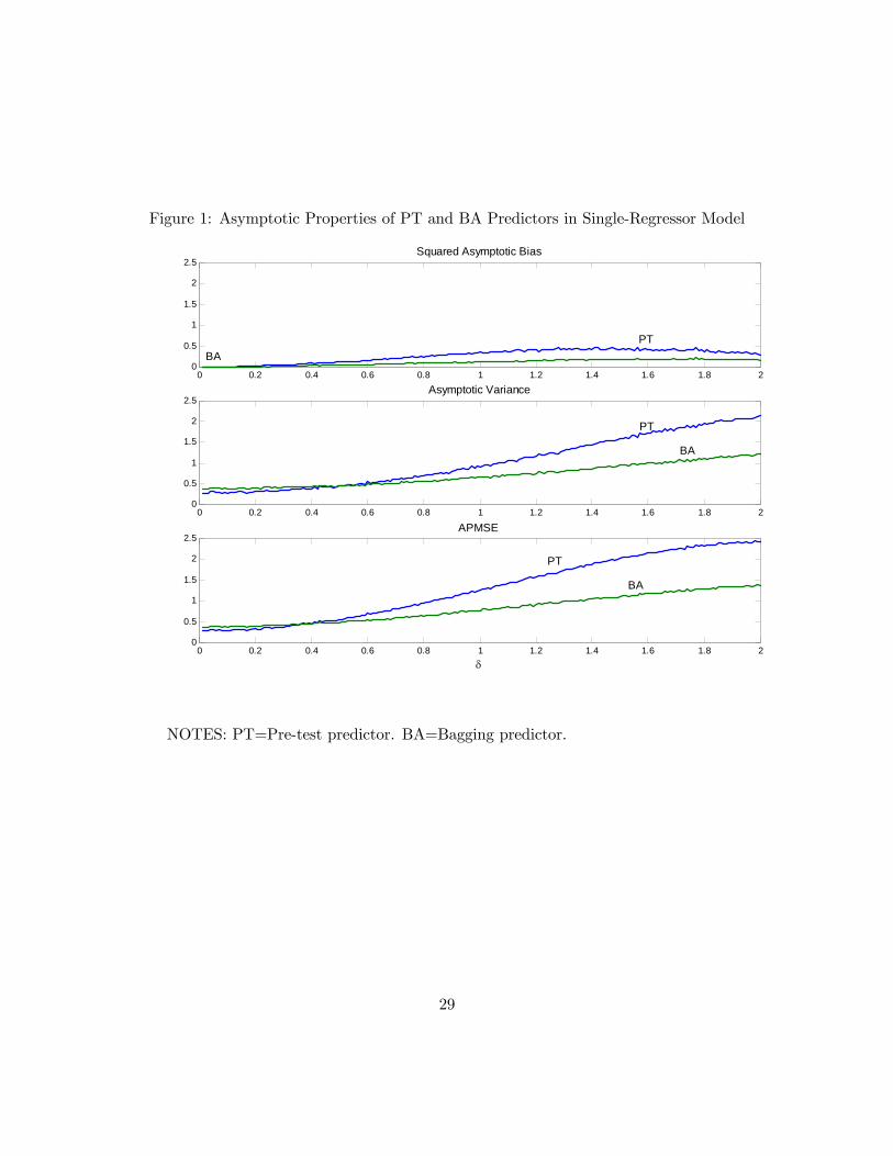
Figure 1: Asymptotic Properties of PT and BA Predictors in Single-Regressor Model

0 0.2 0.4 0.6 0.8 1 1.2 1.4 1.6 1.8 20

0.5

1

1.5

2

2.5Squared Asymptotic Bias

PTBA

0 0.2 0.4 0.6 0.8 1 1.2 1.4 1.6 1.8 20

0.5

1

1.5

2

2.5Asymptotic Variance

PT

BA

0 0.2 0.4 0.6 0.8 1 1.2 1.4 1.6 1.8 20

0.5

1

1.5

2

2.5APMSE

δ

PT

BA

NOTES: PT=Pre-test predictor. BA=Bagging predictor.

29

Figure 2: APMSE of Alternative Predictors in Single-Regressor Model

0 0.2 0.4 0.6 0.8 1 1.2 1.4 1.6 1.8 20

0.5

1

1.5

2

2.5

3

3.5

4

AP

MS

E

δ

BAUR

FR

PT

NOTES: PT=Pre-test predictor. BA=Bagging predictor. UR=Unrestricted predic-tor. FR=Fully restricted predictor

30

Figure 3: APMSE Gains of the BA Predictor Relative to the PT Predictor in Correlated RegressorModel

00.1

0.20.3

0.40.5

0.60.7

0.80.9

0

0.5

1

1.5

21

1.5

2

2.5

ρδ1

PT/

BA

31

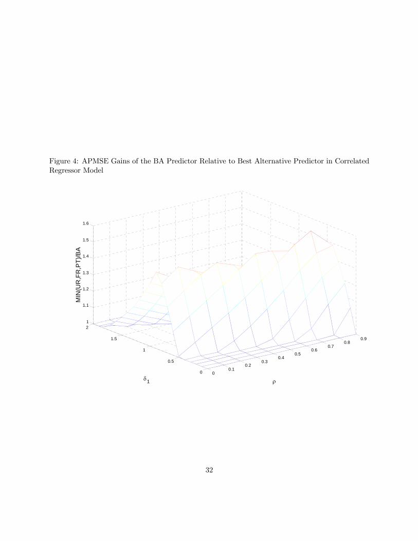
Figure 4: APMSE Gains of the BA Predictor Relative to Best Alternative Predictor in CorrelatedRegressor Model

00.1

0.20.3

0.40.5

0.60.7

0.80.9

0

0.5

1

1.5

21

1.1

1.2

1.3

1.4

1.5

1.6

ρδ1

MIN

(UR

,FR

,PT)

/BA

32

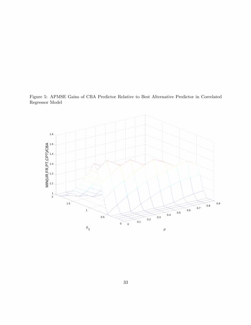
Figure 5: APMSE Gains of CBA Predictor Relative to Best Alternative Predictor in CorrelatedRegressor Model

00.1

0.20.3

0.40.5

0.60.7

0.80.9

0

0.5

1

1.5

21

1.1

1.2

1.3

1.4

1.5

1.6

ρδ1

MIN

(UR

,FR

,PT,

CP

T)/C

BA

33

how useful is bagging in forecasting economic time series ... kilian final version… · how useful...

Documents