how well do monetary fundamentals forecast exchange rates? · how well do monetary fundamentals...
TRANSCRIPT
WORKING PAPER SERIES
How well do monetary fundamentals forecast exchangerates?
Christopher J. Neely and Lucio Sarno
Working Paper 2002-007Ahttp://research.stlouisfed.org/wp/2002/2002-007.pdf
May 2002
FEDERAL RESERVE BANK OF ST. LOUISResearch Division411 Locust Street
St. Louis, MO 63102
______________________________________________________________________________________
The views expressed are those of the individual authors and do not necessarily reflect official positions ofthe Federal Reserve Bank of St. Louis, the Federal Reserve System, or the Board of Governors.
Federal Reserve Bank of St. Louis Working Papers are preliminary materials circulated to stimulatediscussion and critical comment. References in publications to Federal Reserve Bank of St. Louis WorkingPapers (other than an acknowledgment that the writer has had access to unpublished material) should becleared with the author or authors.
Photo courtesy of The Gateway Arch, St. Louis, MO. www.gatewayarch.com
How well do monetary fundamentals forecast exchange rates?
Christopher J. Neely
Lucio Sarno
May 15, 2002
Abstract: For many years after the seminal work of the Meese and Rogoff (1983a), conventionalwisdom held that exchange rates could not be forecast from monetary fundamentals. Monetarymodels of exchange rate determination were generally unable to beat even a naïve no-changemodel in out-of-sample forecasting. More recently, the use of sophisticated econometrictechniques, panel data, and long spans of data has convinced some researchers (Mark and Sul,2001) that monetary models can forecast a small, but statistically significant part of the variationin exchange rates. Others remain sceptical, however (Rapach and Wohar, 2001b; Faust, Rogers,and Wright, 2001). It remains a puzzle why even the most supportive studies find such a smallpredictable component to exchange rates. This article reviews the literature on forecastingexchange rates with monetary fundamentals and speculates as to why it remains so difficult.
Christopher J. Neely is a Research Officer in the Research Department of the Federal Reserve
Bank of St. Louis. Lucio Sarno is a Reader in Financial Economics at Warwick Business
School, the University of Warwick, and a Research Affiliate of the Centre for Economic Policy
Research (CEPR), London. The authors thank Nelson Mark and Jeremy Berkowitz for making
programs and data available and Nelson Mark, David Rapach, and Mark Wohar for helpful
comments on early drafts. Charles Hokayem provided research assistance.
Christopher J. Neely and Lucio Sarno Draft 2 / 5/15/021
INTRODUCTION
In the last decade or so exchange rate economics has seen a number of important
developments, with substantial contributions to both the theory and the empirics of exchange rate
determination. Important developments in econometrics and the increasing availability of high-
quality data have also stimulated a large amount of empirical work on exchange rates. While
this research has improved our understanding of exchange rates, a number of challenges and
questions remain. One of the most widely studied and still unanswered questions in this
literature involves why monetary models of exchange rate determination cannot forecast much of
the variation in exchange rates.
The monetary approach to exchange rate determination emerged as the dominant
exchange rate model at the outset of the recent float in the early 1970s and remains an important
exchange rate paradigm (Frenkel, 1976; Mussa, 1976, 1979; Bilson, 1978). However, Meese
and Rogoff’s (1983a) finding that monetary models’ forecasts could not outperform a simple no-
change forecast was a devastating critique of standard models and marked a watershed in
exchange rate economics. Even with the benefit of twenty years of hindsight, moreover,
evidence that monetary models can consistently and significantly outperform a naïve random
walk is still elusive (e.g. Mark and Sul, 2001; Rapach and Wohar, 2001a and 2001b; Faust,
Rogers, and Wright, 2001).
This article reviews this puzzle and discusses potential explanations for the consistent
failure of monetary models to forecast much variation in nominal exchange rates. We present
the essential elements of the monetary model in the next section, and then discuss, in Section 3,
Christopher J. Neely and Lucio Sarno Draft 2 / 5/15/022
the key empirical studies examining the out-of-sample forecasting performance of the monetary
model. Section 4 outlines possible explanations of the apparent failure of monetary model
predictions and a final section briefly concludes.
THE MONETARY APPROACH TO EXCHANGE RATE DETERMINATION
In this section we describe the main features of the monetary approach to exchange rate
determination in its flexible-price formulation (Frenkel, 1976; Mussa, 1976, 1979).1
The monetary approach starts from the definition of the exchange rate as the relative price of
two monies and attempts to model that relative price in terms of the relative supply of and
demand for those monies. In discrete time, monetary equilibria in the domestic and foreign
country respectively are given by:
(1) tttt iypm λκ −+=
(2) ******tttt iypm λκ −+=
where m, p, y, and i denote the log-levels of the money supply, the price level, income, and the
level of the interest rate, respectively; κ and λ are positive constants; asterisks denote foreign
variables and parameters. In the monetary model, the real interest rate is exogenous in the long
run and determined in world markets, because of the implicit assumption of perfect capital
mobility.
Another building block of the monetary model is absolute purchasing power parity (PPP),
which holds that goods-market arbitrage will tend to move the exchange rate to equalize prices in
Christopher J. Neely and Lucio Sarno Draft 2 / 5/15/023
two countries. For example, if U.S. goods are more expensive than Mexican goods, U.S. and
Mexican consumers will tend to purchase more goods in Mexico and fewer in the United States.
The increased relative demand for Mexican goods will tend to make the peso appreciate with
respect to the dollar and equalize the dollar-denominated prices of U.S. and Mexican goods. The
monetary model assumes that PPP holds continuously, so that:
(3) *ttt pps −=
where st is the log-level of the nominal bilateral exchange rate (the domestic price of the foreign
currency).
The domestic money supply determines the domestic price level and hence the exchange
rate is determined by relative money supplies. Subtracting equation (2) from equation (1),
solving for ( )*tt pp − , and inserting the result into equation (3) provides the solution for the
nominal exchange rate:
(4) )()()( *****ttttttt iiyymms λλκκ −+−−−= ,
which is the fundamental equation of the monetary model. The model is often simplified by
assuming that the income elasticities and interest rate semi-elasticities of money demand are the
same for the domestic and foreign country ( λ = *λ and *κκ = ) so that equation (4) reduces to:
(5) )()()( ***ttttttt iiyymms −+−−−= λκ
According to equation (5), an increase in the domestic money supply relative to the foreign
money stock, for example, induces a depreciation of the domestic currency in terms of the
foreign currency. In other words, the nominal exchange rate, st, increases. Conversely, a boost in
1 For a more comprehensive discussion of the monetary model and other models of exchange ratedetermination, see Sarno and Taylor (2002, Chapters 4 and 5).
Christopher J. Neely and Lucio Sarno Draft 2 / 5/15/024
domestic real income, ceteris paribus, creates an excess demand for the domestic money stock.
In an attempt to increase their real money balances, domestic residents reduce expenditure and
prices fall until money market equilibrium is achieved. Via PPP, the fall in domestic prices (with
foreign prices constant) implies an appreciation of the domestic currency in terms of the foreign
currency (a rise in the value of domestic currency in terms of foreign currency).
The model further assumes that the uncovered interest parity (UIP) condition holds
(6) ( ) )ii(sE *tt1tt −=∆ +
where ∆ is the first-difference operator, so that ∆xt=xt-xt-1 for any x, and Et(∆st+1) denotes the
market expectation of the change in the exchange rate.2 The expected rate of depreciation of the
domestic currency, ∆set+1, can then be substituted for the nominal interest rate differential, (it-i*
t)
in equation (5) to yield:
(7) ( )1tt*tt
*ttt sE)yy()mm(s +∆λ+−κ−−=
Using the identity ( ) ( ) t1tt1tt ssEsE −=∆ ++ , equation (7) may in turn be rewritten as:
(8) ( )1tt1*
tt1*
tt1
t sE)1()yy()1()mm()1(s +−−− λ+λ+−λ+κ−−λ+=
By iterating forward in equation (8), the rational expectations solution to (7) may be written:
(9) [ ])()(1
)1( **
0
1ititititt
i
i
t yymmEs ++++
∞
=
− −−−��
���
�
++= � κ
λλλ
2 Uncovered interest parity (UIP) states that risk-neutral arbitrage will equalize the expected return on aforeign investment—approximately ( )( )*
t1tt isE +∆ + —and the return on a domestic investment ( )ti .
Christopher J. Neely and Lucio Sarno Draft 2 / 5/15/025
where Et[·] denotes the mathematical expectation conditional on the information set available at
time t.3 It is well known from the rational expectations literature, however, that equation (9)
represents only one solution to (7) from a potentially infinite set. In general, given the exchange
rate determined according to equation (9), say sEt, (7) has multiple rational expectations solutions
conforming to:
(10) tEtt Bss +=
where the rational bubble term Bt satisfies
(11) [ ] titt BBE )1(1 λλ += −+
Therefore, sEt simply represents the rational expectations solution to the monetary model in the
absence of rational bubbles. Rational bubbles represent significant departures from the
fundamentals of the model that would not be detected in a specification such as (5). Thus,
testing for the presence of bubbles can be interpreted as an important specification test of the
model (Meese, 1986).
Assumptions of the Monetary Model
Although the simplicity of the flexible-price monetary model is very attractive, this
simplicity requires many assumptions. Open economy macroeconomics is essentially about six
aggregate markets: goods, labor, money, foreign exchange, domestic bonds (i.e. non-money
assets) and foreign bonds. The monetary model concentrates, however, directly on equilibrium
conditions in only one of these markets, the money market. This is implicitly achieved in the
3 Moving from equation (8) to equation (9) requires writing the expression for st+1 in terms of Et+1(st+2)implied by (8), taking expectations, substituting the result for Et(st+1) in (8), and then repeating theprocess for Et+2(st+3), Et+3(st+4), etc.
Christopher J. Neely and Lucio Sarno Draft 2 / 5/15/026
following fashion. By assuming perfect substitutability of domestic and foreign assets, the
domestic and foreign bond markets essentially become a single market, reducing the number of
markets to five. The exchange rate adjusts freely to equilibrate supply and demand in the foreign
exchange market. Perfectly flexible prices and wages likewise equilibrate supply and demand in
the goods and labor markets. Thus, three of the five remaining markets are cleared. Recalling
Walras’ law, according to which equilibrium in n-1 markets of an n-market system implies
equilibrium in the n-th market, equilibrium of the full system in the model is then determined by
equilibrium conditions for the money market. The flexible-price monetary model is thus,
implicitly, a market-clearing general equilibrium model in which continuous PPP among national
price levels is assumed (Sarno and Taylor, 2002 (Chapter 4)).
Sticky-Price Monetary Models
The very high volatility of real exchange rates during the 1970s float, cast serious doubts
on the assumption of continuous PPP and inspired the development of further classes of models,
including sticky-price monetary models and equilibrium models.4
The sticky-price monetary model, due originally to Dornbusch (1976), allows short-term
overshooting of the nominal and real exchange rates above their long-run equilibrium levels. In
4 Equilibrium exchange rate models, due originally to Stockman (1980) and Lucas (1982), analyze thegeneral equilibrium of a two-country model in a representative agent utility maximizing framework withsound microfoundations. Equilibrium models may be viewed as an extension or generalization of theflexible-price monetary model that allows for multiple traded goods and real shocks across countries.These models are not amenable to direct econometric testing or to the formulation of models designed toforecast exchange rates because they are based on utility functions that cannot be directly estimated.(Rather, researchers have sought to test the broad rather than specific implications of this class of models
Christopher J. Neely and Lucio Sarno Draft 2 / 5/15/027
this model, it is assumed that there are “jump variables” in the system (exchange rates and
interest rates) compensating for stickiness in other variables, notably goods prices. Consider the
effects of a cut in the nominal domestic money supply. Since goods prices are sticky in the short
run, this implies an initial fall in the real money supply and a consequent rise in interest rates to
clear the money market. The rise in domestic interest rates then leads to a capital inflow and an
appreciation of the nominal exchange rate. Investors are aware that they are artificially forcing
up the value of the domestic currency and that they may therefore suffer a foreign exchange loss
when the proceeds of their investment are used to repay liabilities in foreign currency.
Nevertheless, as long as the expected foreign exchange loss (the expected rate of depreciation of
the domestic currency) is less than the known capital market gain (the interest rate differential)
risk-neutral investors will continue to borrow abroad to buy domestic assets. A short-run
equilibrium is achieved when the expected rate of depreciation is just equal to the interest rate
differential, i.e. when UIP holds. Since the domestic currency must be expected to depreciate
because of the interest rate differential, the domestic currency must have appreciated beyond its
long-run, PPP equilibrium. In the medium-run, however, domestic prices begin to fall in
response to the fall in the money supply. This alleviates pressure in the money market (the real
money supply rises) and domestic interest rates start to decline. The exchange rate then
depreciates slowly towards long-run PPP. Thus, this model can explain the apparent paradox
that the exchange rate of currencies for countries with relatively higher interest rates tend to
depreciate: the initial interest rate rise induces a sharp exchange rate appreciation, followed by a
slow depreciation as prices adjust, which continues until long-run PPP is satisfied.
for exchange rate behavior.) Similar reasoning applies, at least at the present stage, to the literature on“new open economy macroeconomics” (see Lane, 2001; Sarno, 2001, and the references therein).
Christopher J. Neely and Lucio Sarno Draft 2 / 5/15/028
Nevertheless, it should be clear that, regardless of whether one assumes that prices are
flexible or sticky, the traditional flexible-price monetary model and its sticky-price formulation
imply exactly the same fundamental equation for the exchange rate, which is of the form (5). We
now turn to the empirical evidence on the performance of the monetary model in forecasting
exchange rates.
FORECASTING EXCHANGE RATES WITH MONETARY MODELS
The move to floating exchange rates in the 1970s spawned a wealth of theoretical efforts
to explain their observed high volatility. The monetary models discussed in the previous section
were among the most popular and intuitively appealing. It was natural to examine the empirical
fit and forecasting ability of these models. This section selectively reviews the long literature
attempting to use monetary models to forecast exchange rates.5
Meese and Rogoff (1983a and 1983b)
Meese and Rogoff (1983a, 1983b)—hereafter MR—conducted the seminal work in the
use of monetary models to forecast the exchange rate. Their procedure was straightforward:
They regressed the log of exchange rates on various combinations of relative macroeconomic
5 This paper focuses on forecasting exchange rates with monetary models. There are many non-monetarymodels available, however. Fair (1999) uses a non-monetary macro model; Clarida and Taylor (1997)and Clarida, Sarno, and Taylor (2003) use models based on the term structure; and Evans and Lyons(1999) use order flow models to explain exchange rate changes.
Christopher J. Neely and Lucio Sarno Draft 2 / 5/15/029
variables typically included in the exchange rate models of the 1970s.6 The basic prediction
equation was as follows:
(12) ( ) ( ) ( )
( ) tttte
te
ttttttkt
utbatbaaiiayyammaas
+++−+
−+−+−+=+
**
***
654
3210
ππ,
where st, mt, yt, it, πet, and tbt are the logs of the exchange rate, domestic (U.S.) money supply,
output, interest rates, expected inflation, and the trade balance, at time t. Asterisks denote
foreign variables. MR interpreted exchange rate models, such as the Frenkel-Bilson, Dornbusch-
Frankel and Hooper-Morton models, as implying different sets of restrictions on the coefficients
in the regression (Hooper and Morton, 1982). As is the case with most estimation of
macroeconomic models, little effort was made to explicitly map the model to the functional form
and estimation procedure.
The data were monthly observations from March 1973 through June 1981. MR estimated
the models on in-sample periods by several techniques, including ordinary least squares (OLS),
generalized least squares (GLS), to correct for serial correlation in the errors, and Fair’s (1970)
instrumental variables (IV), to correct for simultaneous equations bias.7 To allow the out-of-
sample forecast coefficients to change, rolling regressions with fixed sample sizes were used.
That is, coefficients were initially estimated using data until November 1976, then 1-, 3-, and 12-
month forecasts were constructed. To construct the next set of forecasts, the next month of data
(December 1976) was added, the first month of data were dropped and the coefficients were
reestimated. For the exercises in which future values of the independent variables were needed
6 MR also estimated univariate models of exchange rate changes and vector autoregressions, employingall the variables in equation (12). These models were also unsuccessful, however, and this paper focuseson efforts with monetary models.7 MR were very thorough in checking the robustness of their results to changes in procedures; because ofspace constraints, it is difficult to list all the permutations of models, estimation methods, and data in thispaper.
Christopher J. Neely and Lucio Sarno Draft 2 / 5/15/0210
to construct forecasts, MR provided the models with actual future values of the independent
variables—instead of forecasting them—to give the monetary model the best possible chance of
forecasting well.8
MR used both in-sample model evaluation criteria, such as the R2, and out-of-sample
criteria, such as the comparison of the root-mean-squared error (RMSE) of the model’s forecast
with that of a benchmark forecast, the driftless random walk. Many of the estimated models fit
the in-sample data well. In-sample evaluation techniques, which permit the use of all the data
available to the researcher, provide more precise estimates of statistics of interest and therefore
have greater power to reject the null hypothesis of no predictability of the exchange rate.9 The
advantage of out-of-sample evaluation procedures is that they implicitly test the stability of the
estimated coefficients and therefore provide a more stringent and realistic hurdle for models to
overcome.
The main conclusion of the MR paper was that none of the structural exchange rate
models were able to forecast out-of-sample better than a naive no-change forecast by mean-
squared-error (MSE) and mean-absolute-error (MAE) criteria. There was some evidence of
predictability at longer horizons, but—given the massive failure at short horizons—this did not
receive much attention.
8 Ironically, Faust, Rogers, and Wright (2001) have recently shown that real-time, Federal Reserveforecasts of future independent money and output variables actually generate better forecasts of the futureexchange rate than do actual future values of the independent variables.9 The power function of a statistical test is the probability of rejecting the null hypothesis, conditional onthe true data generating process. The size of a test is the maximum power under the null hypothesis.
Christopher J. Neely and Lucio Sarno Draft 2 / 5/15/0211
Econometric Problems
The MR exercise had a number of econometric problems, many of which they recognized
and attempted to mitigate with variations on their procedures. First, because the explanatory
variables were all endogenous—determined within the economic system—the estimated
coefficients in the equations surely suffered from simultaneous equations bias. That is, even
with an arbitrarily large amount of data, the coefficient estimates would not converge to any
structural parameters. MR (1983b) attempted to correct for this problem with IV estimation and
an in-sample grid search over possible parameter values. The IV estimation did not help and an
in-sample grid search constituted unconvincing evidence. Because the benchmark no-change
prediction is nested within the model, some combination of parameters must perform at least as
well as the no-change model within the sample. A model with all zeros for coefficients, for
example, will perform exactly as well as the no-change forecast. And, in practice, some
combination of coefficients will almost certainly outperform the no-change forecast, in-sample.
It is unclear, however, why biased coefficients would be a problem for a forecasting
exercise. If the covariance matrix of the structural errors is homoskedastic and stable over time,
forecasts from biased coefficients would be superior to those from structural parameters.
Second, problems with the persistence of the variables in the regression were not dealt
with in a convincing way. (See the boxed insert on persistence and cointegration.) In particular,
because the dependent variable, the log exchange rate, in the predictive regression was probably
Christopher J. Neely and Lucio Sarno Draft 2 / 5/15/0212
I(1), but not cointegrated with any combination of the independent variables, the error term was
probably I(1) and the coefficient estimates were inconsistent, meaningless for forecasting.
More Negative Results
The very strong negative results of the MR study spawned an enormous amount of
subsequent research that varied econometric techniques or the information set to try to rescue the
ability of fundamental models—or any models—to forecast exchange rates. For example, Wolff
(1987, 1988), Schinasi and Swamy (1989), and Canova (1993) used time varying coefficients in
an effort to compensate for instability in the model. Other authors used expanded information
sets or different functional forms for the empirical work (Meese and Rose, 1990). Such efforts,
however, proved immediately unsuccessful or were subsequently shown to be fragile to minor
changes in technique or the data. The MR result that monetary fundamentals do not help predict
exchange rates remained conventional wisdom.
Resurrecting the Monetary Approach: Mark (1995)
Some progress was made, however, in the 1990s. Mark (1995) and Chinn and Meese
(1995) focused on neglected aspects of the problem, primarily the possibility of better long-run
predictability, but also the finite sample properties of the test statistics, and the estimation
procedure implied by the theoretical model.
Mark (1995) considers an expression relating the change in the exchange rate to the
deviation of the exchange rate from a linear combination of relative money and relative output,
Christopher J. Neely and Lucio Sarno Draft 2 / 5/15/0213
which is called the fundamental value of the exchange rate. Essentially Mark exploits the
monetary model equation (5), assuming that κ=1 and the interest differential is equal to zero, so
that the fundamentals term is
(13) ( ) ( )[ ]ttttt yymmf ** −−−=
In this model, the difference between the current fundamentals and the current exchange rate—
called the error correction term ( )tt sf − —determines the k-period ahead change in the exchange
rate:
(14) ( ) tktttkktkt sfss ,++ +−+=− υβα
Using quarterly data on U.S. dollar exchange rates with Canada (CAD), Germany (DEM), Japan
(JPY), and Switzerland (CHF) from 1973:2 to 1991:4, Mark computed the forecast regression in
(14) over horizons of 1, 4, 8, 12, and 16 quarters. Out-of-sample forecasts began in 1984:1.
As did MR, Mark (1995) relied on both in-sample and out-of-sample evidence to assess
the degree of predictability in his model. In-sample evidence included both the statistical
significance of the estimated coefficients, βk, and the R2s of the regressions at various horizons,
Rk2. Out-of-sample evidence focused on the root-mean-squared-error provided by the forecasts
from the estimated model versus those from a driftless random walk, the same out-of-sample
benchmark as used by MR. Mark (1995) examined both the ratio of these RMSEs, OUT/RWk—
also called the Theil U statistic—and the statistical significance of their difference, the DM
statistic (Diebold and Mariano, 1995).10
10 Mark (2001) provides an easily readable discussion of exchange rate forecasting issues.
Christopher J. Neely and Lucio Sarno Draft 2 / 5/15/0214
In evaluating the statistical significance of the results, Mark (1995) confronted some of
the same econometric problems that beset MR. Two of the complications are well known: 1)
Because the independent variable ( )tt sf − is highly autocorrelated, the coefficients αk and βk
would be biased in finite samples (Mankiw and Shapiro, 1986; Stambaugh, 1986); and 2) for
forecast horizons (k) greater than one period, the overlapping forecast errors would have
autocorrelation of at least degree k-1, complicating the construction of functions of the forecast
errors, like coefficient standard errors.
To overcome these difficulties, Mark (1995) relied on nonparametric bootstrapping to
determine the statistical significance of his in-sample and out-of-sample results. Nonparametric
bootstrapping is a method of simulating the distribution of statistics with the distribution of
actual errors estimated by the model—rather than pseudo-random errors from a normal (or other)
distribution—under some assumption about how the data were generated (Berkowitz and Kilian,
2000). In this case, a bootstrapping exercise calculates how often an economy in which there
was no predictability would produce as much support for predictability as found in actual data.
In other words, the question is: Do the real data look like they might have been generated by a
model in which there is no predictability?
Mark (1995) assumed a null data generating process (DGP) where the exchange rate
change is simply a constant plus an error term and the error correction term (ECT) ( )tt sf −
follows an autoregressive process of order P,
(15) tt as ,10 ε+=∆ ,
Christopher J. Neely and Lucio Sarno Draft 2 / 5/15/0215
(16) ( ) ( ) t
P
jjtjtjtt sfbbsf ,2
10 ε+−+=− �
=−− .
Note that (15) implies that the change in the exchange rate is unforecastable. Mark chose the
parameters of the data generating process (DGP) to match the actual data and then constructed
bootstrapped distributions for the test statistics as follows:
1. Estimate the null DGP, which is described by equations (15) and (16).
2. Draw 2000 error samples of size 76 from the estimated null DGP covariance matrix.
3. Use the errors to compute 2000 series of st and ft-st, from equations (15) and (16).
4. Run the predictive regression, equation (14), to obtain estimates of βk, its t-statistics, and the
out-of-sample RMSEs from the estimated models and the benchmark no-change prediction.
Table 1 presents selected results from Mark’s (1995) exercise with significance levels
generated from a DGP described by (15) and (16). Out-of-sample forecasts were evaluated
against the benchmark of a driftless random walk—no change in the exchange rate. Mark (1995)
concluded that evidence of predictability, including βks, adjusted βks, t-statistics, and R2s,
increase with the forecast horizon and that there is evidence of statistically significant
forecastability at horizons of 12 and 16 quarters for the Deutsche mark (DEM) and Swiss franc
(CHF). In the German case, for example, the β1 is 0.035 and the β16 is 1.324. The t-statistics (p-
values) likewise rise (fall) with k, except for Canada. The p-values for the German β1 and β16 t-
statistics are 0.291 and 0.038, respectively. Likewise, the strongest out-of-sample evidence for
predictability is at the longest horizons. The OUT/RW statistics—which are less than one when
the monetary forecasting regression provides lower RMSEs than the no-change forecast—show
that the monetary model beats the benchmark at every horizon for the CHF and the JPY and at
Christopher J. Neely and Lucio Sarno Draft 2 / 5/15/0216
the 12- and 16-quarter horizons for the DEM. In the latter case, the regression’s RMSE is about
½ that of the no-change forecast at the 16-quarter horizon.
Unpredictability Strikes Back
Mark’s (1995) innovative use of the bootstrap solved a number of econometric problems
and appeared to show that there was greater power to predict exchange rates at long horizons
than at short horizons. And, his conclusions were largely buttressed by those of Chinn and
Meese (1995), who investigated many of the same issues and used a wider variety of explanatory
variables, including trade balance, the relative price of tradeables/nontradeables, interest rates,
and inflation, as well as nonparametric methods. Chinn and Meese (1995) found that their
fundamental-based error correction models outperformed the random walk model for long-term
prediction horizons.
Soon, however, other researchers, such as Berkowitz and Giorgianni (2001) and Kilian
(1999) began to criticize Mark’s (1995) methodology and the resultant conclusions. Berkowitz
and Giorgianni (2001) focused on how Mark’s (1995) assumptions about the long run behavior
of the data series influenced the evidence of predictability. Kilian (1999) looked more carefully
at the form of the assumed data generating process and the robustness of the results to changes in
the sample. Both criticisms focused on a disadvantage of bootstrapping and other simulation
procedures: The results can depend crucially on the assumed DGP.
Christopher J. Neely and Lucio Sarno Draft 2 / 5/15/0217
Berkowitz and Giorgianni (2001)—hereafter BG—pointed out that Mark’s (1995)
DGP—equations (15) and (16) in this paper—implicitly assumed that the exchange rate and the
macroeconomic fundamentals were cointegrated, meaning that while each of the series {st, ft}
might be individually I(1), a linear combination of them is stationary, or I(0). In other words,
even if the difference between ft and st is nonstationary in the real data, estimation of equation
(16) will tend to generate data in which the difference between ft and st is stationary. The
generated exchange rate, st, cannot diverge very far from the generated macroeconomic
fundamental, ft. Ex ante, it is not obvious that cointegration is an important issue, as
cointegration is neither a necessary nor sufficient condition for fundamentals to predict exchange
rate changes. However, in this case, BG argue that the distribution of the test statistics depends
on whether there is cointegration or not.11 If the ft and st are not cointegrated in the real data,
then the critical values generated under the assumption of cointegration will be incorrect. The
critical values will be incorrect because the forecasting regression, (14), is almost a spurious
regression (see the boxed insert on persistence) because, as the forecast horizon, k, increases, the
change in the exchange rate, ∆st+k in (14), becomes more persistent and—if there is no
cointegration between st and ft—the independent variable (ft-st) is I(1). When both sides of the
forecasting equation are highly persistent, it approaches a spurious regression, in which
estimated coefficients falsely appear to be statistically significant. More generally, the
distribution of the estimated coefficient from equation (14) will depend on the degree of
persistence in the regressor (ft-st). If the null DGP fails to model the persistence of the regressor
11 Berben and van Dijk (1998) derive the asymptotic distributions of the estimator of the regressionparameter and its t-statistic, under the null hypothesis of no cointegration. They find that the distributiondoes not depend on the forecast horizon; long-horizon regressions have no power advantages in testingfor cointegration. Their analysis shows that Mark’s (1995) results can be at least partly explained by hisassumption of cointegration.
Christopher J. Neely and Lucio Sarno Draft 2 / 5/15/0218
(ft-st) correctly, then the critical values of the forecasting statistics will be wrong and the
inference drawn from the test might be incorrect.
Table 2 presents the results of a Horvath-Watson test (see the boxed insert on persistence)
conducted by BG for cointegration of the exchange rate and macro fundamentals. BG were able
to reject the null of no cointegration for only one rate, the CHF. Kilian’s results were even more
negative toward the cointegration hypothesis; his test failed to reject the null of no cointegration
for any exchange rate.12 Unfortunately, it is often impossible to reject the null of no
cointegration, even if (ft-st) is stationary but persistent. To better evaluate the balance of the
evidence, Kilian adapts an idea of Rudebusch (1993) to weigh the balance of evidence for and
against cointegration.13 Kilian finds that the evidence favors the cointegration hypothesis for the
CHF, was indeterminate for CAD, and favored the null of no cointegration for the DEM and
JPY. Nevertheless, Kilian (1999) concludes that the data are potentially consistent with either the
assumption of cointegration between st and ft or the contrary, no cointegration. He notes that
even if the series are cointegrated, the ECT (ft – st), reverts to its mean very slowly.
Because the Horvath-Watson test results imply that Mark’s (1995) assumption of
cointegration might be incorrect and because this assumption might influence the distribution of
test statistics, BG reexamined the forecastability question without the cointegration assumption.
In particular, BG conducted two bootstrapping experiments to study the behavior of the system
under alternative assumptions about the DGP. Their first model assumed that the exchange rate
12 Kilian’s (1999) Horvath-Watson results might have been different because his sample and estimationmethods were different than BG’s.13 Rudebusch (1993) examines whether one can differentiate the short-run persistence properties under thebest stationary model and the best nonstationary model.
Christopher J. Neely and Lucio Sarno Draft 2 / 5/15/0219
is a random walk with drift—as did Mark (1995)—and that macro fundamentals (ft) follow an
AR(3) process.
(17) tt as ,10 ε+=∆ ,
(18) tj
jtjt fbbf ,2
3
10 ε++= �
=− .
This first model did not assume cointegration and, in generating data, the covariance between the
error terms ε1,t and ε2,t was set equal to zero. The exchange rate and macro fundamentals were
independent by construction.
Table 3, which is excerpted from Table 4 in BG, shows the results of Mark’s forecasting
exercise with three changes: 1) P-values were calculated with the DGP described in (17) and
(18); 2) Parametric bootstrapping was used in place of nonparametric bootstrapping to generate
data; 3) The out-of-sample benchmark included a drift term.14 BG find that many of the DEM
statistics—denoted by shaded boxes—are no longer significant.15 Only the CHF shows much
evidence of predictability.
Table 4—excerpted from Table 5 in BG—is constructed in exactly the same way as
Table 3, except that it extends the sample by three years to the end of 1994. With this change,
there is now no evidence of predictability at the 5% level, even at long horizons for any
exchange rate except the CHF.16 However, there is now evidence of predictability in the
OUT/RW statistics at shorter horizons for the CHF.
14 Kilian (1999) emphasized the importance of a drift in the out-of-sample benchmark, as discussedbelow.15 Tables 3, 4, and 5 show only a subset of the test statistics.16 The overturned results were from t(A) and DM(A, 20) statistics, some of which Table 4 does not show.
Christopher J. Neely and Lucio Sarno Draft 2 / 5/15/0220
The second BG model was an unrestricted vector autoregression (VAR) for the pair {st,
ft}. BG considered this model, which permitted but did not enforce cointegration, as an
intermediate case between the assumption of cointegration enforced by Mark and the assumption
of independence that produced Tables 3 and 4.
(19) t
P
jjtj
P
jjtjt fasaas ,1
12
110 ε+++= ��
=−
=−
(20) t
P
jjtj
P
jjtjt fbsbbf ,2
12
110 ε+++= ��
=−
=− .
The results from the unrestricted VAR—shown in Table 5—show very little evidence of
predictability except for the CHF. BG noted that for the DEM, JPY, and CAD the p-values for
the OUT/RW statistics are smaller at shorter horizons than they are at longer horizons, indicating
less evidence of predictability at longer horizons, in contrast to Mark’s basic conclusion.17
Kilian’s (1999) primary focus was the study of the power function of forecasting
regressions at short horizons versus long horizons rather than foreign exchange predictability per
se. Such a study of power requires a null DGP. Kilian (1999) carefully mapped the monetary
model to a constrained vector error correction model (VECM), which he estimated by feasible
generalized least squares (FGLS) to construct bootstrapping distributions for the forecasting
statistics.
(21) tet uvs ,1+=∆
17 The unrestricted VAR does permit predictability, so the p-values in Table 5 are the probabilities ofobtaining the test statistics, conditional on exchange rates and fundamentals following the estimatedVAR.
Christopher J. Neely and Lucio Sarno Draft 2 / 5/15/0221
(22) [ ] t
p
jjtj
p
jjtjttft ufsfshvf ,2
1
1
221
1
21112 +∆+∆+−−=∆ ��
−
=−
−
=−−− ξξ .
where the system requires h2 < 0 for stability. Kilian notes that while it is asymptotically
equivalent to Mark’s (1995) approximation, (21) and (22) will generate a different small sample
distribution because of the different lag structure and estimation procedure. The results will also
be sensitive to whether the estimated coefficients for the null DGP have been corrected for the
finite-sample bias (see the boxed insert) caused by the persistence of the regressors, which was
not compensated for in Mark’s procedure.
Kilian (1999) also emphasized the importance of the treatment of the drift term in the
forecasting procedures. Specifically, Mark’s inconsistency in permitting a drift in the bootstrap
DGP but not in the benchmark forecast biased the bootstrap critical values. In addition, to
compare a fundamental forecast with drift to a driftless random walk conflates the contributions
of the fundamentals and the drift. That is, if the out-of-sample statistics for the fundamental
model are superior to those of the driftless random walk, one cannot be certain whether it was the
contribution of the fundamentals or just the drift in the monetary model. To isolate the marginal
contribution of the fundamentals, one has to allow for a drift in the benchmark forecast.
To illustrate the importance of the treatment of the drift term, Table 6—excerpted from
the December 1997 working paper version of Kilian (1999)—presents the results from Mark’s
(1995) forecasting exercise using Kilian’s DGP—equations (21) and (22)—with and without a
drift in the random walk. The left-hand panel presents results from the driftless random walk
benchmark while the right-hand panel presents results from the random walk with drift.
Contrasting the results, using a drift in the benchmark eliminates any evidence of predictability
Christopher J. Neely and Lucio Sarno Draft 2 / 5/15/0222
from the JPY case but increases the predictability in the CAD and CHF, especially at short
horizons.
Indeed, both BG and Kilian (1999) took issue with the whole idea of finding
predictability in long-horizon regressions. BG show that there will be no more predictability at
long horizons than at short horizons with a linear model. Kilian (1999) focused on the question
of whether long-horizon regressions truly have greater power to find predictability than short-
horizon tests. In particular, he extended the analytic work done by BG with Monte Carlo
experiments that showed that increasing evidence of predictability at long horizons was due to
the fact that such tests were more likely to err in favor of finding predictability where there was
none, rather than really being better at finding latent predictability. In econometric jargon, the
results were due to size distortions rather than power gains. To summarize: Both BG and Kilian
(1999) conclude that it doesn’t help to increase the forecast horizon if the DGP is linear.
The work of BG and Kilian (1999) shows that the results of the forecasting exercise were
sensitive to a number of factors, including the data sample, the assumption of cointegration in the
DGP, the lag structure of the DGP, the benchmark for out-of-sample comparison, and whether
one corrects the DGP for bias generated by persistent regressors.19 Indeed, their conclusions on
predictability are very similar. BG conclude that failure to impose cointegration leaves only
weak evidence of predictability and that is at predominantly short horizons. Kilian (1999)
similarly concludes that with properly generated critical values, there is some evidence that
19 Groen (1999) also reports the fragility of Mark’s (1995) results to the chosen sample.
Christopher J. Neely and Lucio Sarno Draft 2 / 5/15/0223
monetary fundamentals predict foreign exchange rates but no evidence of more forecastability at
longer horizons.
Panel Studies
When alternative explanations—i.e., predictability or no predictability—seem to fit the
data equally well, employing additional data often illuminates the issue. In the present case, one
might combine evidence from many exchange rates in a panel study of predictability, under the
assumption that the exchange rates are either predictable from fundamentals for all the countries
or predictable for none of them. Groen (2000) and Mark and Sul (2001) aggregated information
about the predictability of exchange rates across countries. Rapach and Wohar (2001b) have
examined whether such aggregation is appropriate.
Groen (2000) examines the question of whether exchange rates are cointegrated with
fundamentals using both rate-by-rate Johansen (1991) cointegration tests and the Levin and Lin
(1993) panel unit root tests on 4 subsets of 14 exchange rates against the U.S. dollar (USD): 1)
all 14; 2) the G-10; 3) the G-7; and 4) the European Monetary System (EMS). The rate-by-rate
Johansen tests reject the null of no cointegration in about 1/3 of the cases using either the USD or
the DEM as numeraire currency; this suggests that “cointegration isn’t widespread.” The more
powerful Levin-Lin (1993) panel test, however, rejects the null of no cointegration jointly for all
the rates at the 5% level, using either the USD or DEM as numeraire for the 14 country panel.20
20 Taylor, Peel, and Sarno (2001) note that panel unit root tests tend to reject the null of a unit root if evenone of the series is stationary, because the null hypothesis is that all of the series have a unit root.
Christopher J. Neely and Lucio Sarno Draft 2 / 5/15/0224
While the results for smaller panels are often insignificant, the overall conclusion is that the most
powerful tests are supportive of cointegration.
The growing consensus against long-horizon prediction regressions and the econometric
complications caused by overlapping forecast errors led Mark and Sul (2001) to eschew the
search for long-run predictability in favor of a one-period ahead panel regression of quarterly
data on 18 exchange rates and fundamentals. The sample started in 1973:1 and ended in 1997:1.
Mark and Sul (2001) first test for and find evidence of cointegration with a panel dynamic OLS
framework, which controls for asymptotic bias in the forecast statistics. This cointegration
finding is used to construct the bootstrapped data that corrects coefficients for persistent
regressor bias and evaluates the statistical significance of Theil U statistics. The forecasting
equation is the multi-exchange rate analogue to those used in previous papers, a one-period
ahead panel regression, estimated by seemingly unrelated regressions (SUR) over expanding
samples.21 The system could be written as follows:
(23) ( ) 1,,,,1, ++ +−=− tititititi sfss εβ
1,11, +++ ++= tititi uθγε ,
where si,t, fi,t are the log exchange rate and the log fundamentals of exchange rate i at time t, γi is
an exchange rate specific error, θt is a time specific error and ui,t is an idiosyncratic error. Three
exchanges rates are considered as numeraire for the system: the USD, the CHF, and the JPY. In
the one-step ahead forecasting exercises, Mark and Sul (2001) find that monetary fundamentals
have a small but statistically significant amount of predictability—using Theil U statistics—
21 In expanding samples, one-period is added to the in-sample data used to estimate coefficients beforeeach forecast to give the model the maximum amount of data with which to construct out-of-sampleforecasts.
Christopher J. Neely and Lucio Sarno Draft 2 / 5/15/0225
when the USD or CHF is numeraire but none when the JPY is the standard. They also find that
monetary fundamentals predict somewhat better than PPP fundamentals.
Both the Groen (2000) and Mark and Sul (2001) studies pooled data across countries to
try to bring more power to answering the question of how well monetary models predict the
exchange rate? The practice of pooling data across countries assumes, of course, that the same
data generating process produces the data for all the countries. Such assumptions are called
“homogeneity assumptions.” If the data generating process is different across countries,
however, then falsely pooling the data can lead to incorrect inference. Using the Mark and Sul
(2001) data set, Rapach and Wohar (2001b) first confirm previous results that the monetary
model fits very poorly in country-by-country estimation during the floating rate period (1973:1-
1997:1). “It is difficult to overstate how poorly the monetary model performs…on a country by
country basis” (Rapach and Wohar, 2001b, p. 3). In contrast, however, pooled estimates do
support the monetary model, as in Mark and Sul (2001). Next, the authors formally test whether
the cross-country homogeneity assumptions are justified. That is, is it likely that one data
generating process could have produced the disparate coefficient estimates from the 14 different
exchange rates? A Wald test rejects this one-DGP hypothesis for most subsets of countries
(Mark, Ogaki, and Sul, 2000). And a Monte Carlo study shows that it is very plausible that
heterogeneous data generating processes—fit to the 14 exchange rate/fundamental processes—
could produce pooled parameter estimates similar to those found in the real data. These findings
cast doubt on the wisdom of pooling data across countries or the reliability of the conclusions.
Christopher J. Neely and Lucio Sarno Draft 2 / 5/15/0226
Arguing in favor of pooling, however, is the fact that the pooled parameter estimates are
as good as the country-by-country forecasts at short horizons and better at long horizons.
Rapach and Wohar (2001b) cite Pesaran, Shin and Smith (1999) as arguing that omitted
variables and measurement error might lead to the false rejection of homogeneity restrictions and
that pooling might still be appropriate and helpful under such circumstances. Ultimately, Rapach
and Wohar (2001b) conclude that researchers could reasonably differ about the fit of the
monetary model of exchange rates during the Post-Bretton Woods period.
Long Spans of Data
Combining evidence from many countries in a panel study is one way to increase the
available data to determine whether exchange rates are cointegrated with fundamentals. Another
approach is to simply use much longer spans of data. Rapach and Wohar (2001a) took this latter
approach, using exchange rate, money, and output data from 14 industrialized countries, over a
span as long as 115 years (1880-1995), to investigate the long run relationship between these
variables. Table 7 summarizes the results from Rapach and Wohar (2001a).
First, Rapach and Wohar (2001a) noted that if exchange rates are to be predicted from
relative money and output, some combination of the three variables {st, (mt-mt*), (yt-yt
*)} must be
stationary (I(0)). If no combination is I(0), then the error from any forecast will become
arbitrarily big as time goes on, bigger than the benchmark error. If one of these variables {st,
(mt-mt*), (yt-yt
*)} is I(1), for example, while the other 2 are I(0), then no linear combination can
be I(0) and the monetary model can be rejected. Such unit root tests alone enable the authors to
reject the monetary model for Denmark, Norway, and Sweden (Table 7, column 3).
Christopher J. Neely and Lucio Sarno Draft 2 / 5/15/0227
Second, Rapach and Wohar (2001a) go on to estimate cointegrating vectors—using 4
different methods—for the following equation:
(24) ( ) ( ) tttttt yymms εβββ +−+−+= *2
*10
and test—using 4 different cointegration tests—whether those vectors are consistent with the
vector implied by the simple monetary model {β1 = 1, β2 = -1}(Table 7, columns 4 and 5).22 All
4 tests find evidence of cointegration for France, Spain, and Italy; 2 tests find evidence for
Finland and Portugal; and 1 test finds evidence for Belgium and Switzerland. The estimated
coefficients are often close to those implied by the simple monetary model {β1 = 1, β2 = -1}.
Third, the authors use unit root tests on the residuals from the error correction term
( ) ( ){ }**ttttt yymms −+−− , which is implied by the simple monetary model. A rejection of the
unit root hypothesis is interpreted as supporting the “simple,” “long-run” monetary model. The
tests produce strong support for the monetary model for the Netherlands, France, Italy, and
Spain, moderate support for Belgium, Finland and Portugal and weak support for Switzerland
(Table 7, column 6). The authors caution, however, that deviations from monetary fundamentals
can be substantial and very persistent.
22 Rapach and Wohar (2001b) defined exchange rates to be the foreign currency price of domesticcurrency—the inverse of the definition used previously in this paper—and defined the fundamentals asthe negative of Mark’s fundamentals. For consistency, this paper will use Mark’s definitions of theexchange rate and fundamentals. Also, note that Rapach and Wohar (2001b) imposed β2 = 0 in theirestimate of the cointegrating vector for Finland and Portugal because relative output was found to be I(0)in those cases.
Christopher J. Neely and Lucio Sarno Draft 2 / 5/15/0228
Fourth, a vector error-correction model is estimated to investigate the dynamics of the
relation between exchange rates and the fundamentals. The VECM model can be written as
follows:
(25) ( ) t
p
iiti
p
iitittt fbsasfs ,11
11111 εµλ ++∆+∆+−=∆ ��
=−
=−−−
(26) ( ) t
p
iiti
p
iitittt fdscsff ,22
11112 εµλ ++∆+∆+−=∆ ��
=−
=−−−
Note that fundamentals predict exchange rates in the expected way if either λ1 > 0 or 0bP
1ii >�
=
.
Similarly, exchange rates predict fundamentals in the expected way if either λ2 < 0 or 0cP
1ii >�
=
.
Rapach and Wohar (2001a) find that the error correction term ( )11 −− − tt sf predicts exchange
rates for Belgium, Finland, and Italy ( )0 ,0 21 => λλ . In VECM jargon, monetary fundamentals
are said to be weakly exogenous for these cases. For Portugal and Spain, the exchange rate is
weakly exogenous, the error correction term predicts future fundamental changes but not
exchange rate changes ( )0 ,0 21 <= λλ . The error correction term predicts both future
fundamentals and exchange rate changes for France and Switzerland ( )0 ,0 21 <> λλ . These
results are summarized in columns 7 and 8 of Table 7.
Finally, the authors pursue the usual out-of-sample forecasting exercises and find that
their Theil U statistics, DM statistics, and encompassing regressions show evidence of
predictability—beyond the random walk with drift—for Belgium, Italy, and Switzerland, and
Christopher J. Neely and Lucio Sarno Draft 2 / 5/15/0229
some evidence for Finland (from encompassing regressions not shown in Table 7).23 Not
surprisingly, cases in which the VECM showed the exchange rate to be weakly exogenous are
out-of-sample forecasting failures. The authors note, however, that forecasting failure can still
be consistent with the long-run monetary model if deviations from fundamentals predict future
fundamentals (Table 7, column 9).
Figure 1 uses the case in the which the monetary model has the best out-of-sample fit —
the case of the U.S. dollar/Italian lira (USD/ITL)—to illustrate how little of the variation in the
one-year ahead exchange rate change the monetary model predicts. The top panel shows
exchange rate changes and recursive, out-of-sample forecasts from 1939 to the end of the sample
in 1995. The bottom panel shows the same data from the beginning of the floating exchange rate
era, 1973-1995. The chart appears to show that the monetary model forecasts best in extreme
circumstances, such as those seen during the high inflation that Italy suffered during World War
II or during 1986-1987, when the dollar weakened again after a period of unusual strength. In
almost all periods, however, the monetary model explains very little of the variation in one-year
ahead exchange rate changes.
Data revisions
Faust, Rogers, and Wright (2001) examine the impact of yet another issue: data revisions.
Previous studies had all assumed that the data they used would be fixed and known to a
forecaster. In fact, macroeconomic data such as money supply and output figures are often
extensively revised, meaning that data depends on the date on which the series were obtained. In
23 An encompassing regression evaluates the predictive content of forecasting techniques by testingwhether realized values of the exchange rate depend positively on predicted values from one or more
Christopher J. Neely and Lucio Sarno Draft 2 / 5/15/0230
other words, if one obtained U.S. output data in April 1992—as the authors infer that Mark did—
one might have a different estimate of U.S. output growth for 1991:1 than if one obtained data in
April 1993. To investigate the effect of data revisions on forecasting exercises with monetary
models, Faust, Rogers, and Wright (2001) obtained 38 data sets, representing the best estimates
of the data as it stood on different dates from April 1988 to October 2000.
With these 38 data sets, they first attempted to see if they would obtain the same
inference as Mark (1995) by holding back the final 40 quarters of data from each set for an out-
of-sample forecasting exercise. That is, each of the 38 data sets were different from each other
both because of data revisions and the fact that the final 40 quarters of data would be over
different periods. They found that the only vintages of the data that would have produced
significant long-horizon predictability were those in a 2-year window around April 1992, the
time that Mark collected his data set. The decrease in predictability for other data sets was due
to both sample periods—as noted by Kilian (1999)—and data revisions.
To isolate the marginal effect of data revisions, the authors fixed the sample period and
compared results using more and less revised data. The more-revised data showed less evidence
of predictability. Theil U-statistics rise and p-values fall as the data are revised. For example,
data revisions made the 16Q Theil U statistic rise from 0.52 to 0.64 in the German case and from
0.55 to 0.69 in the Japanese case. And the p-values for these cases rise above 0.1. Similarly, the
authors estimate a portfolio-balance model using inflation, interest rates and cumulated trade
balances—as in Chinn and Meese (1995)—and they find that data revisions have even larger
effects than in the monetary model.
forecasting techniques.
Christopher J. Neely and Lucio Sarno Draft 2 / 5/15/0231
Next Faust, Rogers, and Wright (2001) investigate the quality of “real-time” data
forecasts. Real-time forecasts use the latest revision of data available at any given point in time
to estimate the parameters of the model and make forecasts. That is, real-time exercises can use
a different set of data for each forecast period. In contrast, the other forecasting exercises (e.g.,
Mark, 1995) used one data set—the latest revisions available when the research is done—to
estimate the equation and make forecasts. Faust, Rogers, and Wright find that real-time data
provides better out-of-sample predictive power—according to out-of-sample relative RMSEs—
in almost every case than the latest data revision. Perhaps this should not surprise us. If the
exchange rate changes do depend on market participants expectations of future monetary
fundamentals (i.e., equation (14)), which are based on currently available (real-time) data, then
real-time data should provide better estimates of market expectations.
Finally, the authors find that Federal Reserve forecasts of future variables sometimes
outperform actual future values of those independent variables in a MR-type regression multi-
period forecast. This is ironic. MR sought to give the monetary models the best possible chance
to forecast well by replacing forecasts of future independent variables with actual values. But,
(at least some) forecasts of fundamentals predict exchange rates better than the future values of
those variables.
The study concludes that both the particular sample period used by Mark (1995) and the
particular vintage of data revisions combined to produce better out-of-sample forecasting
performance than most data samples and/or data revisions would have. Indeed, only data sets
Christopher J. Neely and Lucio Sarno Draft 2 / 5/15/0232
constructed in about 1992 would have shown evidence of long-horizon predictability. Faust,
Rogers, and Wright (2001) speculate that evidence of forecastability is actually an artifact of data
mining, the tendency to test multiple models on one set of data until, by chance, positive results
are found. Finally, for a given fixed sample, real-time data would have produced better forecasts
than the latest data revisions. Hindsight turns out to handicap the forecasts rather than to
improve them.
Nonlinear models
The monetary model is intuitively appealing but clearly explains very little exchange rate
variability. One explanation for the weak relation is that exchange rates are relatively insensitive
to monetary fundamentals close to equilibrium values but tend to strongly revert to those
fundamentals when the deviation is large. Taylor and Peel (2000), Taylor, Peel, and Sarno
(2001) and Kilian and Taylor (2001) investigate the plausibility of this characterization with
nonlinear models.
Taylor and Peel (2000) estimate a nonlinear error correction model of quarterly exchange
rates and monetary fundamentals for the pound/dollar (GBP/USD) and Deutchesmark/dollar
(DEM/USD) exchange rates from 1973:1 to 1996:4. They find that the exponential smooth
transition autoregressive (ESTAR) model (Granger and Terävirta, 1993) parsimoniously
describes the deviation of the exchange rate from monetary fundamentals. This model predicts
that the exchange rate change will nearly be unpredictable when the deviation from fundamentals
is small, but will strongly revert toward those fundamentals when the deviation is big. The
Christopher J. Neely and Lucio Sarno Draft 2 / 5/15/0233
authors use this to characterize the degree of over- and undervaluation of the exchange rates
during the modern period of floating exchange rates. Similarly, Taylor, Peel, and Sarno (2001)
show that the same model fits real exchange rates well and explains deviations from purchasing
power parity.
Kilian and Taylor (2001) note that a convincing explanation for the nonlinear dynamics
of the ESTAR model is lacking. The authors suggest a candidate model in which uncertainty
about the fundamental value of the exchange rate deters agents from speculating against small
deviations from fundamentals.24 Monte Carlo studies show that there is more predictability for
plausible DGPs at the one- and two-year horizons, so long horizon tests are useful in such an
environment. Further, if the ESTAR model is the true DGP, then all past tests of long-horizon
predictability are invalid because they assume a linear null data generating process, which is
incorrect. Consistent with this prediction, the authors find that in-sample evidence of
predictability from seven OECD countries increases “dramatically” with the forecast horizon.25
Yet, the authors are still unable to find evidence of out-of-sample predictability. They ascribe
this to the low power of out-of-sample tests, given the short span of post-Bretton Woods data and
the rarity of large departures from fundamentals during that time.
24 Kilian and Taylor (2001) assume that the fundamental value is a function of relative prices rather thanmoney and output, as in the monetary model.25 Mark and Sul (2002) find that long-horizon regressions can have asymptotic power advantages overone-period-ahead procedures in cases similar to those found in foreign exchange forecasting. TheirMonte Carlo experiments show that the phenomenon might be even more common in finite samples.
Christopher J. Neely and Lucio Sarno Draft 2 / 5/15/0234
WHY DOESN'T THE MONETARY MODEL PREDICT WELL?
One obvious problem is that three of the building blocks of the monetary model, money
demand equations, purchasing power parity (PPP), and uncovered interest parity (UIP) do not
work very well (Engel, 1996; Engel, 2000). Money demand equations have proven unstable,
especially in the United States (Friedman and Kuttner, 1992), but changing the numeraire
currency doesn’t seem to help the monetary model much.
But that begs the question as to why PPP and UIP perform so poorly. Why are floating
exchange rates so volatile and unrelated to prices and interest differentials? Many researchers
have claimed that volatile expectations or departures from rationality are likely to account for the
failure of exchange rate models. For example, Frankel (1999) argues that exchange rates are
detached from fundamentals by swings in expectations about future values of the exchange rate.
These fluctuations in exchange rates are essentially bubbles, of the type discussed in Section 2.
Four pieces of evidence suggest that expectations are to blame for such behavior: 1) Survey
measures of exchange rate expectations are very poor forecasters and the expectations,
themselves, are frequently not internally consistent (Frankel and Froot, 1987; Sarno and Taylor
2001); 2) Failure of expectations to be rational is often blamed for the failure of UIP (Engel,
1996); 3) Trend following trading rules appear to make risk-adjusted excess returns, in apparent
violation of the efficient markets hypothesis (Neely, 1997; Neely, Weller, and Dittmar, 1997); 4)
Switching from a fixed exchange rate to a floating rate—which changes the way expectations are
formed—changes the behavior of nominal and real exchange rates and the ability of UIP to
explain exchange rate changes.
Christopher J. Neely and Lucio Sarno Draft 2 / 5/15/0235
This latter point requires some explanation. Fixed exchange rates anchor investor
sentiment about the future value of a currency because of the government’s commitment to
stabilize its value. If expectations are based on fundamentals, rather than irrationally changing
expectations, then the relationship between fundamentals and exchange rates should be the same
under a fixed exchange rate regime as it is under a floating regime. This is not the case.
Countries that move from floating exchange rates to fixed exchange rates experience a dramatic
change in the relationship between prices and exchange rates. Specifically, real exchange rates
(exchange rates adjusted for inflation in both countries) are much more volatile under floating
exchange rate regimes, where expectations are not tied down by promises of government
intervention (Mussa, 1986). Figure 2 illustrates a typical case: When the German government
ceased to fix the DEM to the USD in March 1973, the variability in the real DEM/USD exchange
rate increased dramatically. This result suggests that, contrary to the efficient markets
hypothesis, swings in investor expectations may detach exchange rates from fundamental values
in the short run. Similarly, UIP seems to do such a poor job explaining USD exchange rates
while doing a pretty good job with semi-fixed rates such as those found in the EMS (Flood and
Rose, 1996). Indeed, Flood and Rose (1999) develop a UIP-based model of the exchange rate
that explains why UIP—and exchange rate forecasts—might perform poorly in the short term
even with perfect rational agents.
Christopher J. Neely and Lucio Sarno Draft 2 / 5/15/0236
CONCLUSION: THE BIG PICTURE
The seminal work of MR showed that monetary models were unable to forecast exchange
rates better than a no-change forecast. Since then, a small army of researchers has attempted to
forecast exchange rates with the analytically attractive monetary model. Initial attempts were
strikingly unsuccessful; Mark (1995), however, appeared to show that monetary fundamentals
could predict exchange rate changes at 3-4 year horizons. Kilian (1999), Berkowitz and
Giorgianni (2001), and Faust, Rogers, and Wright (2001) subsequently criticized the underlying
assumptions of Mark’s study with respect to the stationarity of the data, robustness to sample
period, appropriate benchmark for comparison, and the vintage of the data. Attempts to forecast
with panel studies (Mark and Sul, 2001; Rapach and Wohar, 2001b) or very long samples
(Rapach and Wohar, 2001a) have failed to establish the existence of predictability beyond
reasonable doubt.
Other research suggests that exchange rates might be nonlinearly mean reverting to
fundamentals and that the intuitively appealing monetary model might therefore provide better
predictions when exchange rates deviate substantially from fundamentals (Kilian and Taylor,
2001). Such models also imply that long-horizon regressions might be more informative than
short-horizon regressions.
How should one interpret these disparate results? The monetary model is intuitively
appealing and monetary variables likely influence exchange rate changes. But, like all models, it
simplifies reality. The literature on exchange rate forecasting has shown that the amount of
Christopher J. Neely and Lucio Sarno Draft 2 / 5/15/0237
exchange rate variation explained by monetary models is—at most—small. Further research will
doubtless continue to attempt to quantify this predictability. Other future research might
profitably explore the way that expectations of asset prices are formed and the factors—like
dispersion of belief, risk aversion, and transactions costs—that permit extreme nominal exchange
rate variability by hindering arbitrage.
Other conclusions that one might draw depend on the purpose of these forecasting
exercises, which is little discussed in the literature. Researchers have usually motivated their
work by the desire to evaluate monetary models of the exchange rate (MR) and have cautioned
that they are not trying to build the best possible forecasting model (Mark and Sul, 2001), but the
negative results for monetary models have nonetheless produced a conventional wisdom in the
profession that exchange rate changes cannot be forecast—or cannot be forecast using
macroeconomic fundamentals. It is not clear, however, that this is true.
It might seem obvious that both policy makers and firms would want to forecast
exchange rates, but it isn’t entirely clear why they would wish to do so with monetary
fundamentals. Policymakers might wish to forecast exchange rates because of their influence on
variables of more direct interest such as output and inflation. But why not directly forecast
output and inflation if that is the case? Or, firms might wish to forecast exchange rates to make
asset allocation decisions. But that would require a forecast of deviations from UIP, not of
exchange rates themselves. Surely the reason for exchange rate forecasts will influence the
method of evaluation and the value of those projections. Future research should address this
topic.
Christopher J. Neely and Lucio Sarno Draft 2 / 5/15/0238
REFERENCES
Berben, Robert-Paul and van Dijk, Dick. “Does the Absence of Cointegration Explain the
Typical Findings in Long Horizon Regressions?” Unpublished manuscript. Tinbergen
Institute, April 6, 1998.
Berkowitz, Jeremy and Giorgianni, Lorenzo. “Long-Horizon Exchange Rate Predictability?”
Review of Economics and Statistics, February 2001, 83(1), pp. 81-91.
Berkowitz, Jeremy and Kilian, Lutz. “Recent Developments in Bootstrapping Time Series.”
Econometric Reviews, February 2000, 19(1), pp. 1-48.
Bilson, John F.O. “Rational Expectations and the Exchange Rate,” in Jacob A. Frenkel and
Henry G. Johnson, eds., The Economics of Exchange Rates: Selected Studies, Reading,
MA: Addison-Wesley Press,1978.
Blough, Stephen R. “The Relationship Between Power and Level for Generic Unit Root Tests in
Finite Samples.” Journal of Applied Econometrics, July-Sept. 1992, 7(3), pp. 295-308.
Canova, Fabio. “Modelling and Forecasting Exchange Rates with a Bayesian Time-Varying
Coefficient Model.” Journal of Economic Dynamics and Control, January-March 1993,
17(1/2), pp. 233-261.
Chinn, Menzie D. and Meese, Richard A. “Banking on Currency Forecasts: How Predictable Is
Change in Money?” Journal of International Economics, February 1995, 38(1/2), pp.
161-78.
Clarida, Richard H. and Taylor, Mark P."The Term Structure of Forward Exchange Premiums
and The Forecastability of Spot Exchange Rates: Correcting the Errors." Review of
Economics and Statistics, 1997, 79(3), pp. 353-61.
Christopher J. Neely and Lucio Sarno Draft 2 / 5/15/0239
Clarida, Richard H.; Sarno, Lucio; Taylor, Mark P. and Valente, Giorgio."The Out-of-Sample
Success of Term Structure Models as Exchange Rate Predictors: A Step Beyond."
Journal of International Economics, 2003, (forthcoming).
Diebold, Francis X. and Mariano, Roberto S. “Comparing Predictive Accuracy.” Journal of
Business and Economic Statistics, July 1995, 13(3), pp. 253-63.
Dornbusch, Rudiger. “Expectations and Exchange Rate Dynamics.” Journal of Political
Economy, December 1976, 84(6), pp. 1161-76.
Engel, Charles. “Long-Run PPP May Not Hold After All.” Journal of International Economics,
August 2000, 51(2), pp. 243-73.
Engel, Charles. “The Forward Discount Anomaly and the Risk Premium: A Survey of Recent
Evidence.” Journal of Empirical Finance, June 1996, 3(2), pp. 123-92.
Evans, M.D.D. and R.K. Lyons. "Order Flow and Exchange Rate Dynamics." Unpublished
manuscript, Georgetown University, December 1999.
Fair, Ray C. “The Estimation of Simultaneous Equation Models with Lagged Endogenous
Variables and First Order Serially Correlated Errors.” Econometrica, May 1970, 38(3),
pp. 507-16.
Fair, Ray C. “Evaluating the Information Content and Money Making Ability of Forecasts from
Exchange Rate Equations.” Unpublished manuscript, Yale University, May 1999.
Faust, Jon. “Near Observational Equivalence and Unit Root Processes: Formal Concepts and
Implications.” Board of Governors of the Federal Reserve System International Finance
and Economics Discussion Paper: 447, 1993.
Faust, Jon R.; John H. Rogers, and Wright, Jonathan H. “Exchange Rate Forecasting: The Errors
We’ve Really Made.” International Finance Discussion Paper 714, December 2001.
Christopher J. Neely and Lucio Sarno Draft 2 / 5/15/0240
Flood, Robert P. and Rose, Andrew K. “Fixes: Of the Forward Discount Puzzle.” Review of
Economics and Statistics, November 1996, 78(4), pp.748-52.
Flood, Robert P. and Rose, Andrew K. “Understanding Exchange Rate Volatility Without the
Contrivance of Macroeconomics.” Economic Journal, November 1999, 109(459), pp.
F660-72.
Frankel, Jeffrey. “How Well Do Foreign Exchange Markets Work: Might a Tobin Tax Help?” in
Mahbub ul Haq, Inge Kaul, and Isabelle Grunberg, eds., The Tobin Tax: Coping with
Financial Volatility. New York and Oxford: Oxford University Press, 1996.
Frankel, Jeffrey A. and Froot, Kenneth A. “Using Survey Data to Test Standard Propositions
Regarding Exchange Rate Expectations.” American Economic Review, March 1987,
77(1), pp. 133-53.
Frenkel, Jacob A. “A Monetary Approach to the Exchange Rate: Doctrinal Aspects and
Empirical Evidence.” Scandinavian Journal of Economics, 1976, 78(2), pp. 200-224.
Friedman, Benjamin M. and Kuttner, Kenneth N.“Money, Income, Prices, and Interest Rates.”
American Economic Review, June 1992, 82(3), pp. 472-92.
Granger, C.W.J. and Newbold, P. “Spurious Regressions in Econometrics.” Journal of
Econometrics, July 1974, 2(2), pp. 111-20.
Granger, Clive W.J. and Teräsvirta, Timo. Modelling Nonlinear Economic Relationships.
Oxford: Oxford University Press, 1993.
Groen, Jan J.J. “The Monetary Exchange Rate Model as a Long-Run Phenomenon.” Journal of
International Economics, December 2000, 52(2), pp. 299-319.
Groen, Jan J.J. “Long-Run Predictability of Exchange Rates: Is It For Real?” Empirical
Economics, August 1999, 24(3), pp. 451-69.
Christopher J. Neely and Lucio Sarno Draft 2 / 5/15/0241
Hooper, Peter and Morton, John E. “Fluctuations in the Dollar: A Model of Nominal and Real
Exchange Rate Determination.” Journal of International Money and Finance, April
1982, 1, pp. 39-56.
Horvath, Michael T.K. and Watson, Mark W. “Testing for Cointegration When Some of the
Cointegrating Vectors Are Prespecified.” Econometric Theory, December 1995, 11(5),
pp. 984-1014.
Johansen, Soren. “Estimation and Hypothesis Testing of Cointegration Vectors in Gaussian
Vector Autoregressive Models.” Econometrica, November 1991, 59(6), pp. 1551-80.
Kendall, M.G. “Note on Bias in the Estimation of Autocorrelation.” Biometrika, December 1954,
41(3/4), pp. 403-4.
Kilian, Lutz. “Exchange Rates and Monetary Fundamentals: What Do We Learn From Long-
Horizon Regressions?” Journal of Econometrics, September/October 1999, 14(5), pp.
491-510.
Kilian, Lutz and Taylor, Mark. “Why Is It So Difficult to Beat Random Walk Forecasts of
Exchange Rates?” Unpublished manuscript, October 2001.
Lane, Philip R. “The New Open Economy Macroeconomics: A Survey.” Journal of
International Economics, August 2001, 54(2), pp. 235-66.
Levin, Andrew and Lin, Chien-Fu. “Unit Root Tests in Panel Data: New Results.” University of
California, San Diego Department of Economics Working Paper: 93-56, December 1993.
Lucas, Robert E. “Interest Rates and Currency Prices in a Two-Country World.” Journal of
Monetary Economics, November 1982, 10(3), pp. 335-59.

Christopher J. Neely and Lucio Sarno Draft 2 / 5/15/0242
Mankiw, N. Gregory and Shapiro, Matthew D. “Do We Reject Too Often? Small Sample
Properties of Tests of Rational Expectations Models.” Economics Letters, 1986, 20, pp.
139-45.
Mark, Nelson C. International Macroeconomics and Finance: Theory and Econometric
Methods. Malden, MA: Blackwell Publishers, 2001.
Mark, Nelson C. “Exchange Rates and Fundamentals: Evidence on Long-Horizon
Predictability.” American Economic Review, March 1995, 85(1), pp. 201-18.
Mark, Nelson C. and Sul, Donggyu. “Nominal Exchange Rates and Monetary Fundamentals:
Evidence from a Small Post-Bretton Woods Panel.” Journal of International Economics,
February 2001, 53(1), pp. 29-52.
______________ and _____________. “Asymptotic Power Advantages of Long Horizon
Regressions.” Unpublished manuscript, Ohio State University, April 2002.
Mark, Nelson C.; Ogaki, Masao and Sul, Donggyu. “Dynamic Seemingly Unrelated
Cointegrating Regression.” Unpublished manuscript, Ohio State University, July 5, 2000.
Marriott, F.H.C. and Pope, J.A. “Bias in the Estimation of Autocorrelations.” Biometrika,
December 1954, 41(3/4), pp. 390-402.
Meese, Richard A. “Testing for Bubbles in Exchange Markets: A Case of Sparkling Rates?”
Journal of Political Economy, April 1986, 94(2), pp. 345-73.
Meese, Richard A. and Rogoff, Kenneth. “Empirical Exchange Rate Models of the Seventies: Do
They Fit Out of Sample?” Journal of International Economics, February 1983a, 14(1/2),
pp. 3-24.
Christopher J. Neely and Lucio Sarno Draft 2 / 5/15/0243
______________ and _____________. “The Out-of-Sample Failure of Empirical Exchange Rate
Models: Sampling Error or Misspecification?” in Jacob Frenkel, ed., Exchange Rates and
International Macroeconomics. Chicago: NBER and University of Chicago Press, 1983b.
Meese, Richard A. and Rose, Andrew K. “Nonlinear, Nonparametric, Nonessential Exchange
Rate Estimation.” American Economic Review, May 1990, 80(2), pp.192-96.
Mussa, Michael. “The Exchange Rate, the Balance of Payments and Monetary and Fiscal Policy
under a Regime of Controlled Floating.” Scandinavian Journal of Economics, 1976,
78(2), pp. 229-48.
Mussa, Michael. “Empirical Regularities in the Behavior of Exchange Rates and Theories of the
Foreign Exchange Market,” in Karl Brunner and Allan H. Meltzer, eds., Carnegie-
Rochester Conference Series on Public Policy: Policies for Employment, Prices and
Exchange Rates, Vol. 11, 1979.
Mussa, Michael. “Nominal Exchange Rate Regimes and the Behavior of Real Exchange Rates:
Evidence and Implications,” in Karl Brunner and Allan H. Meltzer, eds., Carnegie-
Rochester, Conference Series on Public Policy: Real Business Cycles, Real Exchange
Rates, and Actual Policies, Vol. 25, Autumn 1986, pp. 117-214.
Neely, Christopher J. “Technical Analysis in the Foreign Exchange Market: A Layman’s Guide.”
Federal Reserve Bank of St. Louis Review, September/October 1997, 79(5), pp. 23-38.
Neely, Christopher; Weller, Paul; and Dittmar, Rob. “Is Technical Analysis in the Foreign
Exchange Market Profitable? A Genetic Programming Approach.” Journal of Financial
and Quantitative Analysis, December 1997, 32(4), pp. 405-26.
Christopher J. Neely and Lucio Sarno Draft 2 / 5/15/0244
Pesaran, M. Hashem; Shin, Yongcheol and Smith, Ron P. "Pooled Mean Group Estimation of
Dynamic Heterogeneous Panels." Journal of the American Statistical Association, June
1999, 94(446), pp. 621-34.
Phillips, Peter C. B. “Understanding Spurious Regressions in Econometrics.” Journal of
Econometrics, December 1986, 33(3), pp. 311-40.
Rapach, David E. and Wohar, Mark E. “Testing the Monetary Model of Exchange Rate
Determination: New Evidence from a Century of Data.” Unpublished manuscript,
November 2001a, Journal of International Economics (forthcoming).
Rapach, David E. and Wohar, Mark E. “Testing the Monetary Model of Exchange Rate
Determination: A Closer Look at Panels.” September 2001b.
Rudebusch, Glenn D. “The Uncertain Unit Root in Real GNP.” American Economic Review,
March 1993, 83(1), pp. 264-72.
Sarno, Lucio. “Toward a New Paradigm in Open Economy Modeling: Where Do We Stand?”
Federal Reserve Bank of St. Louis Review, May/June 2001, 83(3), pp. 21-36.
Sarno, Lucio and Taylor, Mark P. “The Microstructure of the Foreign Exchange Market: A
Selective Survey of the Literature.” Princeton Studies in International Economics, No. 89,
April 2001.
Sarno, Lucio and Taylor, Mark P. The Economics of Exchange Rates. Cambridge and New York:
Cambridge University Press, 2002 (forthcoming).
Schinasi, Garry J. and Swamy, P.A.V.B. “The Out-of-Sample Forecasting Performance of
Exchange Rate Models When Coefficients Are Allowed to Change.” Journal of
International Money and Finance, September 1989, 8(3), pp. 375-90.
Christopher J. Neely and Lucio Sarno Draft 2 / 5/15/0245
Stambaugh, Robert F. “Bias In Regressions With Lagged Stochastic Regressors.” Working Paper
No. 156, Center for Research in Security Prices, January 1986.
Stock, James H. and Watson, Mark W. “A Simple Estimator of Cointegrating Vectors in Higher
Order Integrated Systems.” Econometrica, July 1993, 61(4), pp. 783-820.
Stockman, Alan C. “A Theory of Exchange Rate Determination.” Journal of Political Economy,
August 1980, 88(4), pp. 673-98.
Taylor, Mark P. and Peel, David A. “Nonlinear Adjustment, Long-Run Equilibrium and
Exchange Rate Fundamentals.” Journal of International Money and Finance, February
2000, 19(1), pp. 33-53.
Taylor, Mark P.; Peel, David A. and Sarno, Lucio. "Nonlinear Mean-Reversion in Real
Exchange Rates: Towards a Solution to the Purchasing Power Parity Puzzles."
International Economic Review 2001, 42(4), pp. 1015-42.
Wolff, Christian C.P. “Time-Varying Parameters and the Out-of-Sample Forecasting
Performance of Structural Exchange Rate Models.” Journal of Business and Economic
Statistics, January 1987, 5(1), pp. 87-97.
Wolff, Christian C.P. “Exchange Rates, Innovations and Forecasting.” Journal of International
Money and Finance, March 1988, 7(1), pp. 49-61.
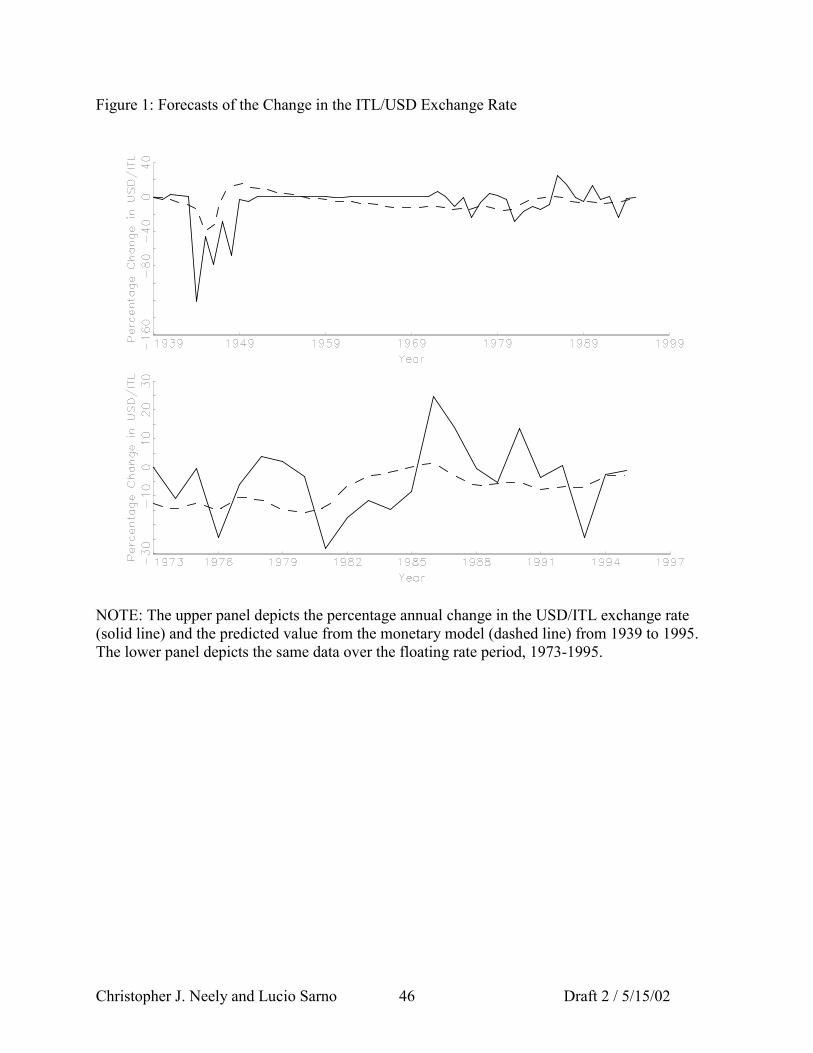
Christopher J. Neely and Lucio Sarno Draft 2 / 5/15/0246
Figure 1: Forecasts of the Change in the ITL/USD Exchange Rate
NOTE: The upper panel depicts the percentage annual change in the USD/ITL exchange rate(solid line) and the predicted value from the monetary model (dashed line) from 1939 to 1995.The lower panel depicts the same data over the floating rate period, 1973-1995.
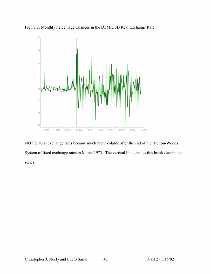
Christopher J. Neely and Lucio Sarno Draft 2 / 5/15/0247
Figure 2: Monthly Percentage Changes in the DEM/USD Real Exchange Rate.
NOTE: Real exchange rates became much more volatile after the end of the Bretton-Woods
System of fixed exchange rates in March 1973. The vertical line denotes this break date in the
series.
Christopher J. Neely and Lucio Sarno Draft 2 / 5/15/0248
Boxed Insert: A Short Primer on Persistence and Cointegration
A data series is said to be stationary if neither its mean nor any of its autocovariances
depend on the date t. An implication of this is that the series will tend to be mean-reverting, to
tend to return to its expected value when it departs from it. The longer such a series takes to
return to its mean, the more persistent it is said to be. A series that is infinitely persistent will
never tend to return to any mean value—its expected value doesn’t exist; such a series is
nonstationary.26 Note that if a variable Xt has zero mean and is uncorrelated at all leads and
lags—i.e., it is white noise—then Xt is stationary. If we define Yt as the cumulated sums of Xt
( �=
=t
iit XY
0
), then, as t → ∞, the variance of Yt becomes infinite, Yt does not tend to revert to any
value, so it is nonstationary. Yt is also said to be I(1), integrated of order one—because it is the
partial sum (or integral) of the Xis—and X is referred to as I(0). Yt is also sometimes called a
random walk because changes to it are unpredictable (random) from other
information, ttt XYY += −1 , ( ) 0=∆ tYE . Note that if Xt had a constant non-zero mean, that is
ttX εδ += , where εt is white noise, then Yt would be random walk with drift: ttt YY εδ ++= −1 ,
( ) δ=∆ tYE .
If at least one linear combination of I(1) variables is I(0), the variables are said to be
cointegrated. Economic theory often implies that a linear combination of variables will be
stationary. For example, one version of purchasing power parity says that exchange rates should
be cointegrated with relative price levels—assuming that both are I(1) variables.
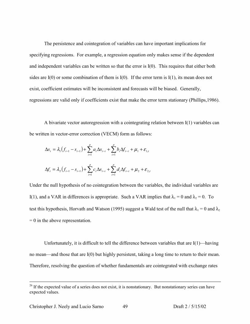
Christopher J. Neely and Lucio Sarno Draft 2 / 5/15/0249
The persistence and cointegration of variables can have important implications for
specifying regressions. For example, a regression equation only makes sense if the dependent
and independent variables can be written so that the error is I(0). This requires that either both
sides are I(0) or some combination of them is I(0). If the error term is I(1), its mean does not
exist, coefficient estimates will be inconsistent and forecasts will be biased. Generally,
regressions are valid only if coefficients exist that make the error term stationary (Phillips,1986).
A bivariate vector autoregression with a cointegrating relation between I(1) variables can
be written in vector-error correction (VECM) form as follows:
( ) t
p
iiti
p
iitittt fbsasfs ,11
11111 εµλ ++∆+∆+−=∆ ��
=−
=−−−
( ) t
p
iiti
p
iitittt fdscsff ,22
11112 εµλ ++∆+∆+−=∆ ��
=−
=−−−
Under the null hypothesis of no cointegration between the variables, the individual variables are
I(1), and a VAR in differences is appropriate. Such a VAR implies that λ1 = 0 and λ2 = 0. To
test this hypothesis, Horvath and Watson (1995) suggest a Wald test of the null that λ1 = 0 and λ2
= 0 in the above representation.
Unfortunately, it is difficult to tell the difference between variables that are I(1)—having
no mean—and those that are I(0) but highly persistent, taking a long time to return to their mean.
Therefore, resolving the question of whether fundamentals are cointegrated with exchange rates
26 If the expected value of a series does not exist, it is nonstationary. But nonstationary series can haveexpected values.
Christopher J. Neely and Lucio Sarno Draft 2 / 5/15/0250
is more difficult than one might think. In fact, it can be shown that stationary and nonstationary
processes are observationally equivalent (Blough, 1992; Faust,1993). In other words, there is a
nonstationary process that will behave arbitrarily close to any given stationary process, and vice
versa. In practice, it is frequently the case that a series of interest could be consistent with either
stationarity or nonstationarity.
The problem of spurious regression occurs when an I(1) variable is regressed on an
unrelated I(1) variable. Spurious regressions, investigated by Granger and Newbold (1974) and
analyzed further by Phillips (1986), are regressions that relate independent random walks and
produce apparently statistically significant—but inconsistent and meaningless—coefficients.
Intuitively, spurious regressions occur because the moment matrix of the regressors (X’X)
doesn’t converge to anything and so becomes arbitrarily large, making the reported standard
error of the coefficient too small and permitting false rejections of the hypothesis that the
coefficient is equal to zero.
Even a variable that is not I(1) can cause problems in a regression if it is persistent—
highly autocorrelated. It has long been understood that if the independent variable in a
regression is persistent, the coefficient estimates in that regression will be biased. Marriott and
Pope (1954) and Kendall (1954) studied the phenomenon in the autoregressive case and Mankiw
and Shapiro (1986) and Stambaugh (1986) extended the results to multiple equation models. To
understand why persistence creates finite sample bias, consider the case of an AR(1) process:
ttt yy εβ += −1 where 00 =y and ( ) 22 σε =tE and ( ) 0=tE ε . The OLS estimator is given by
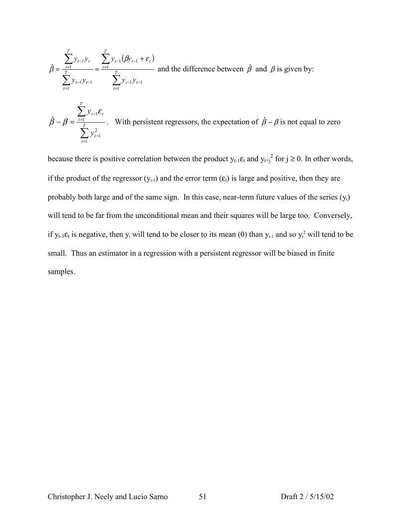
Christopher J. Neely and Lucio Sarno Draft 2 / 5/15/0251
( )
�
�
�
�
=−−
=−−
=−−
=− +
== T
ttt
T
tttt
T
ttt
T
ttt
yy
yy
yy
yy
111
111
111
11
ˆεβ
β and the difference between β̂ and β is given by:
�
�
=−
=−
=− T
tt
T
ttt
y
y
1
21
11
ˆε
ββ . With persistent regressors, the expectation of ββ −ˆ is not equal to zero
because there is positive correlation between the product yt-1εt and yt+j2 for j ≥ 0. In other words,
if the product of the regressor (yt-1) and the error term (εt) is large and positive, then they are
probably both large and of the same sign. In this case, near-term future values of the series (yt)
will tend to be far from the unconditional mean and their squares will be large too. Conversely,
if yt-1εt is negative, then yt will tend to be closer to its mean (0) than yt-1 and so yt2 will tend to be
small. Thus an estimator in a regression with a persistent regressor will be biased in finite
samples.
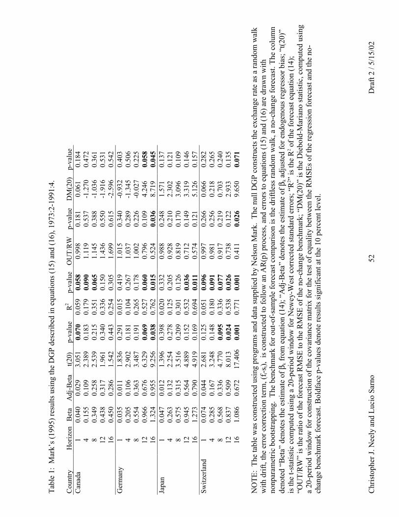
Chr
isto
pher
J. N
eely
and
Luc
io S
arno
D
raft
2 / 5
/15/
0252
Tabl
e 1:
Mar
k’s (
1995
) res
ults
usi
ng th
e D
GP
desc
ribed
in e
quat
ions
(15)
and
(16)
, 197
3:2-
1991
:4.
Cou
ntry
Hor
izon
Bet
aA
dj-B
eta
t(20)
p-va
lue
R2
p-va
lue
OU
T/R
Wp-
valu
eD
M(2
0)p-
valu
eC
anad
a1
0.04
00.
029
3.05
10.
070
0.05
90.
058
0.99
80.
181
0.06
10.
184
40.
155
0.10
92.
389
0.18
30.
179
0.09
01.
119
0.53
7-1
.270
0.47
28
0.34
90.
258
2.53
90.
215
0.35
10.
065
1.14
50.
388
-1.0
360.
361
120.
438
0.31
71.
961
0.34
00.
336
0.15
01.
436
0.55
0-1
.916
0.53
116
0.45
00.
286
1.54
20.
443
0.25
40.
305
1.69
90.
615
-2.5
960.
542
Ger
man
y1
0.03
50.
011
1.83
60.
291
0.01
50.
419
1.01
50.
340
-0.9
320.
403
40.
205
0.10
62.
902
0.18
10.
104
0.26
71.
037
0.28
9-1
.345
0.50
68
0.55
40.
363
3.48
70.
191
0.26
50.
178
1.00
20.
226
-0.0
270.
225
120.
966
0.67
66.
329
0.06
90.
527
0.06
00.
796
0.10
94.
246
0.05
816
1.32
40.
955
9.25
60.
038
0.76
20.
015
0.52
40.
036
8.71
90.
045
Japa
n1
0.04
70.
012
1.39
60.
398
0.02
00.
332
0.98
80.
248
1.57
10.
137
40.
263
0.13
22.
254
0.27
80.
125
0.20
50.
928
0.21
02.
302
0.12
18
0.57
50.
315
3.51
60.
209
0.30
10.
126
0.81
90.
170
3.09
60.
109
120.
945
0.56
44.
889
0.15
20.
532
0.03
60.
712
0.14
93.
319
0.14
616
1.27
30.
790
4.91
90.
169
0.69
40.
011
0.57
40.
121
5.12
60.
157
Switz
erla
nd1
0.07
40.
044
2.68
10.
125
0.05
10.
096
0.99
70.
266
0.06
60.
282
40.
285
0.16
73.
248
0.14
80.
180
0.09
10.
981
0.25
60.
218
0.26
58
0.56
80.
336
4.77
00.
095
0.33
60.
077
0.91
70.
219
0.70
30.
240
120.
837
0.50
98.
013
0.02
40.
538
0.02
60.
738
0.12
22.
933
0.13
516
1.08
60.
672
17.4
060.
001
0.77
10.
001
0.41
10.
026
9.65
00.
071
NO
TE:
The
tabl
e w
as c
onst
ruct
ed u
sing
pro
gram
s and
dat
a su
pplie
d by
Nel
son
Mar
k. T
he n
ull D
GP
cons
truct
s the
exc
hang
e ra
te a
s a ra
ndom
wal
kw
ith d
rift,
the
erro
r cor
rect
ion
term
, (f t-
s t),
is c
onst
ruct
ed to
follo
w a
n A
R(p
) pro
cess
, and
err
ors t
o eq
uatio
ns (1
5) a
nd (1
6) a
re d
raw
n w
ithno
npar
amet
ric b
oots
trapp
ing.
The
ben
chm
ark
for o
ut-o
f-sa
mpl
e fo
reca
st c
ompa
rison
is th
e dr
iftle
ss ra
ndom
wal
k, a
no-
chan
ge fo
reca
st. T
he c
olum
nde
note
d “B
eta”
den
otes
the
estim
ate
of β
k fro
m e
quat
ion
(14)
; “A
dj-B
eta”
den
otes
the
estim
ate
of β
k adj
uste
d fo
r end
ogen
ous r
egre
ssor
bia
s; “
t(20)
”is
the
t-sta
tistic
com
pute
d us
ing
a 20
-per
iod
win
dow
for N
ewey
-Wes
t cor
rect
ed st
anda
rd e
rror
s; “
R2 ”
is th
e R
2 of t
he fo
reca
st e
quat
ion
(14)
;“O
UT/
RW
” is
the
ratio
of t
he fo
reca
st R
MSE
to th
e R
MSE
of t
he n
o-ch
ange
ben
chm
ark;
“D
M(2
0)”
is th
e D
iebo
ld-M
aria
no st
atis
tic, c
ompu
ted
usin
ga
20-p
erio
d w
indo
w fo
r con
stru
ctio
n of
the
cova
rianc
e m
atrix
for t
he te
st o
f equ
ality
bet
wee
n th
e R
MSE
s of t
he re
gres
sion
fore
cast
and
the
no-
chan
ge b
ench
mar
k fo
reca
st. B
oldf
ace
p-va
lues
den
ote
resu
lts si
gnifi
cant
at t
he 1
0 pe
rcen
t lev
el.
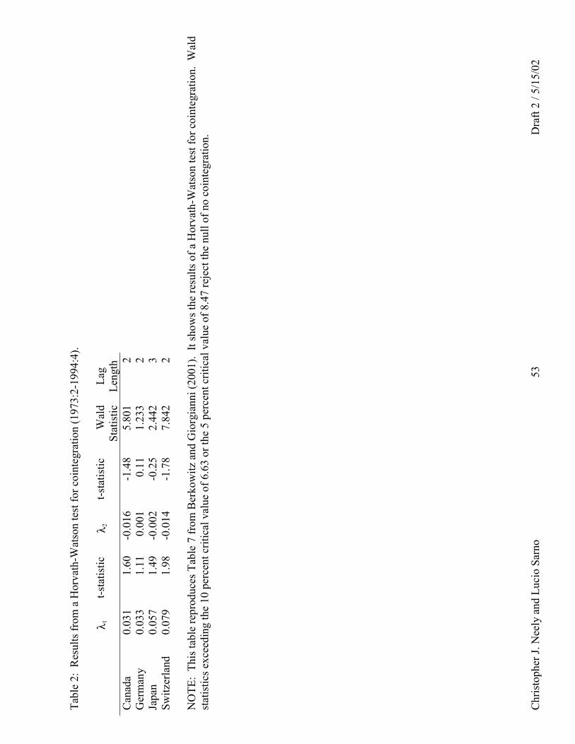
Chr
isto
pher
J. N
eely
and
Luc
io S
arno
D
raft
2 / 5
/15/
0253
Tabl
e 2:
Res
ults
from
a H
orva
th-W
atso
n te
st fo
r coi
nteg
ratio
n (1
973:
2-19
94:4
).
λ 1t-s
tatis
ticλ 2
t-sta
tistic
Wal
dSt
atis
ticLa
gLe
ngth
Can
ada
0.03
11.
60-0
.016
-1.4
85.
801
2G
erm
any
0.03
31.
110.
001
0.11
1.23
32
Japa
n0.
057
1.49
-0.0
02-0
.25
2.44
23
Switz
erla
nd0.
079
1.98
-0.0
14-1
.78
7.84
22
NO
TE:
This
tabl
e re
prod
uces
Tab
le 7
from
Ber
kow
itz a
nd G
iorg
iann
i (20
01).
It sh
ows t
he re
sults
of a
Hor
vath
-Wat
son
test
for c
oint
egra
tion.
Wal
dst
atis
tics e
xcee
ding
the
10 p
erce
nt c
ritic
al v
alue
of 6
.63
or th
e 5
perc
ent c
ritic
al v
alue
of 8
.47
reje
ct th
e nu
ll of
no
coin
tegr
atio
n.
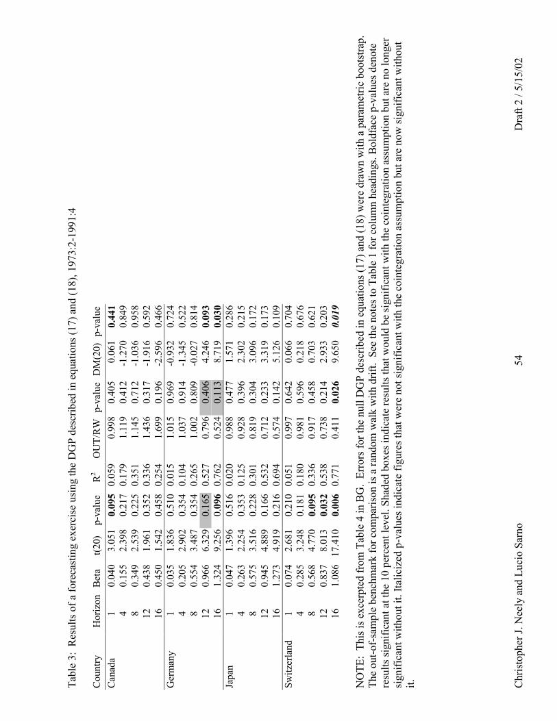
Chr
isto
pher
J. N
eely
and
Luc
io S
arno
D
raft
2 / 5
/15/
0254
Tabl
e 3:
Res
ults
of a
fore
cast
ing
exer
cise
usi
ng th
e D
GP
desc
ribed
in e
quat
ions
(17)
and
(18)
, 197
3:2-
1991
:4
Cou
ntry
Hor
izon
Bet
at(2
0)p-
valu
eR
2O
UT/
RW
p-va
lue
DM
(20)
p-va
lue
Can
ada
10.
040
3.05
10.
095
0.05
90.
998
0.40
50.
061
0.44
14
0.15
52.
398
0.21
70.
179
1.11
90.
412
-1.2
700.
849
80.
349
2.53
90.
225
0.35
11.
145
0.71
2-1
.036
0.95
812
0.43
81.
961
0.35
20.
336
1.43
60.
317
-1.9
160.
592
160.
450
1.54
20.
458
0.25
41.
699
0.19
6-2
.596
0.46
6G
erm
any
10.
035
1.83
60.
510
0.01
51.
015
0.96
9-0
.932
0.72
44
0.20
52.
902
0.35
40.
104
1.03
70.
914
-1.3
450.
522
80.
554
3.48
70.
354
0.26
51.
002
0.80
9-0
.027
0.81
412
0.96
66.
329
0.16
50.
527
0.79
60.
406
4.24
60.
093
161.
324
9.25
60.
096
0.76
20.
524
0.11
38.
719
0.03
0Ja
pan
10.
047
1.39
60.
516
0.02
00.
988
0.47
71.
571
0.28
64
0.26
32.
254
0.35
30.
125
0.92
80.
396
2.30
20.
215
80.
575
3.51
60.
228
0.30
10.
819
0.30
43.
096
0.17
212
0.94
54.
889
0.16
60.
532
0.71
20.
233
3.31
90.
173
161.
273
4.91
90.
216
0.69
40.
574
0.14
25.
126
0.10
9Sw
itzer
land
10.
074
2.68
10.
210
0.05
10.
997
0.64
20.
066
0.70
44
0.28
53.
248
0.18
10.
180
0.98
10.
596
0.21
80.
676
80.
568
4.77
00.
095
0.33
60.
917
0.45
80.
703
0.62
112
0.83
78.
013
0.03
20.
538
0.73
80.
214
2.93
30.
203
161.
086
17.4
100.
006
0.77
10.
411
0.02
69.
650
0.01
9
NO
TE:
This
is e
xcer
pted
from
Tab
le 4
in B
G.
Erro
rs fo
r the
nul
l DG
P de
scrib
ed in
equ
atio
ns (1
7) a
nd (1
8) w
ere
draw
n w
ith a
par
amet
ric b
oots
trap.
The
out-o
f-sa
mpl
e be
nchm
ark
for c
ompa
rison
is a
rand
om w
alk
with
drif
t. S
ee th
e no
tes t
o Ta
ble
1 fo
r col
umn
head
ings
. Bol
dfac
e p-
valu
es d
enot
ere
sults
sign
ifica
nt a
t the
10
perc
ent l
evel
. Sha
ded
boxe
s ind
icat
e re
sults
that
wou
ld b
e si
gnifi
cant
with
the
coin
tegr
atio
n as
sum
ptio
n bu
t are
no
long
ersi
gnifi
cant
with
out i
t. Ita
liciz
ed p
-val
ues i
ndic
ate
figur
es th
at w
ere
not s
igni
fican
t with
the
coin
tegr
atio
n as
sum
ptio
n bu
t are
now
sign
ifica
nt w
ithou
tit.
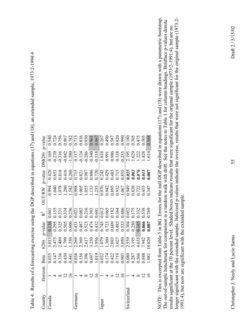
Chr
isto
pher
J. N
eely
and
Luc
io S
arno
D
raft
2 / 5
/15/
0255
Tabl
e 4:
Res
ults
of a
fore
cast
ing
exer
cise
usi
ng th
e D
GP
desc
ribed
in e
quat
ions
(17)
and
(18)
, an
exte
nded
sam
ple,
197
3:2-
1994
:4
Cou
ntry
Hor
izon
Bet
at(2
0)p-
valu
eR
2O
UT/
RW
p-va
lue
DM
(20)
p-va
lue
Can
ada
10.
035
3.01
30.
136
0.04
10.
994
0.42
80.
169
0.54
04
0.14
72.
475
0.29
50.
155
1.04
00.
853
-0.2
700.
724
80.
336
2.48
90.
325
0.33
11.
078
0.81
8-0
.316
0.75
612
0.43
01.
799
0.50
50.
334
1.28
00.
416
-0.8
420.
967
160.
441
1.35
00.
606
0.23
61.
542
0.26
0-1
.580
0.78
2G
erm
any
10.
038
2.26
90.
431
0.02
10.
998
0.71
50.
117
0.71
34
0.15
62.
369
0.48
70.
082
1.00
50.
821
-0.1
240.
836
80.
396
2.61
70.
523
0.21
61.
055
0.98
7-0
.286
0.93
012
0.69
73.
250
0.47
40.
393
1.13
30.
886
-0.3
400.
961
161.
019
3.95
60.
432
0.60
11.
235
0.72
0-0
.518
0.96
7Ja
pan
10.
032
1.07
90.
745
0.01
20.
976
0.24
21.
818
0.26
74
0.17
41.
360
0.72
30.
065
0.94
20.
429
0.99
10.
490
80.
422
2.09
30.
609
0.18
20.
895
0.48
50.
986
0.58
712
0.71
93.
027
0.48
50.
364
0.93
20.
715
0.33
80.
820
160.
907
3.05
00.
533
0.48
61.
067
0.85
5-0
.235
0.99
0Sw
itzer
land
10.
080
2.55
90.
304
0.05
20.
949
0.03
52.
195
0.18
04
0.28
73.
195
0.25
00.
175
0.83
80.
063
1.62
90.
305
80.
566
4.63
50.
165
0.33
20.
722
0.07
61.
222
0.47
512
0.84
87.
942
0.06
60.
538
0.45
50.
015
1.42
80.
505
161.
081
18.8
200.
007
0.76
90.
347
0.00
71.
614
0.56
8
NO
TE:
This
is e
xcer
pted
from
Tab
le 5
in B
G. E
rror
s for
the
null
DG
P de
scrib
ed in
equ
atio
ns (1
7) a
nd (1
8) w
ere
draw
n w
ith a
par
amet
ric b
oots
trap.
The
out-o
f-sa
mpl
e be
nchm
ark
for c
ompa
rison
is a
rand
om w
alk
with
drif
t. S
ee th
e no
tes t
o Ta
ble
1 fo
r col
umn
head
ings
. Bol
dfac
e p-
valu
es d
enot
ere
sults
sign
ifica
nt a
t the
10
perc
ent l
evel
. Sh
aded
box
es in
dica
te re
sults
that
wer
e si
gnifi
cant
for t
he o
rigin
al sa
mpl
e (1
973:
2-19
91:4
), bu
t are
no
long
er si
gnifi
cant
with
the
exte
nded
sam
ple.
Ital
iciz
ed p
-val
ues i
ndic
ate
the
reve
rse,
resu
lts th
at w
ere
not s
igni
fican
t for
the
orig
inal
sam
ple
(197
3:2-
1991
:4),
but n
ow a
re si
gnifi
cant
with
the
exte
nded
sam
ple.
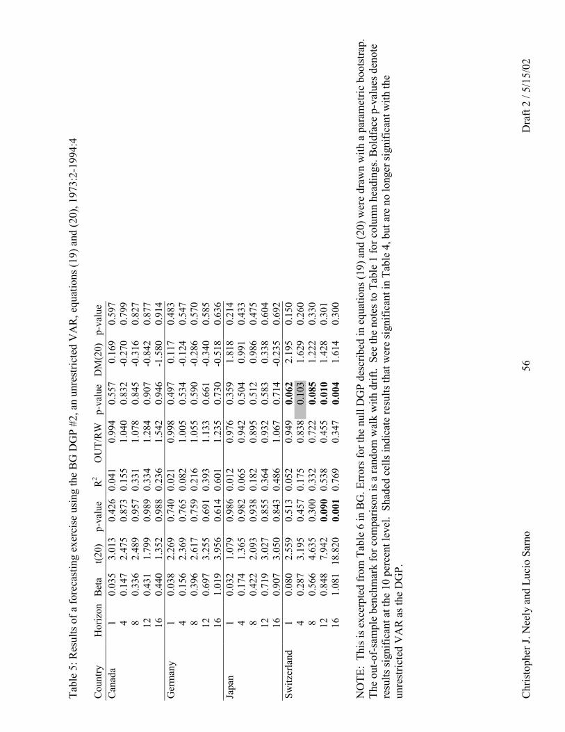
Chr
isto
pher
J. N
eely
and
Luc
io S
arno
D
raft
2 / 5
/15/
0256
Tabl
e 5:
Res
ults
of a
fore
cast
ing
exer
cise
usi
ng th
e B
G D
GP
#2, a
n un
rest
ricte
d V
AR
, equ
atio
ns (1
9) a
nd (2
0), 1
973:
2-19
94:4
Cou
ntry
Hor
izon
Bet
at(2
0)p-
valu
eR
2O
UT/
RW
p-va
lue
DM
(20)
p-va
lue
Can
ada
10.
035
3.01
30.
426
0.04
10.
994
0.55
70.
169
0.59
74
0.14
72.
475
0.87
30.
155
1.04
00.
832
-0.2
700.
799
80.
336
2.48
90.
957
0.33
11.
078
0.84
5-0
.316
0.82
712
0.43
11.
799
0.98
90.
334
1.28
40.
907
-0.8
420.
877
160.
440
1.35
20.
988
0.23
61.
542
0.94
6-1
.580
0.91
4G
erm
any
10.
038
2.26
90.
740
0.02
10.
998
0.49
70.
117
0.48
34
0.15
62.
369
0.76
50.
082
1.00
50.
534
-0.1
240.
547
80.
396
2.61
70.
759
0.21
61.
055
0.59
0-0
.286
0.57
012
0.69
73.
255
0.69
10.
393
1.13
30.
661
-0.3
400.
585
161.
019
3.95
60.
614
0.60
11.
235
0.73
0-0
.518
0.63
6Ja
pan
10.
032
1.07
90.
986
0.01
20.
976
0.35
91.
818
0.21
44
0.17
41.
365
0.98
20.
065
0.94
20.
504
0.99
10.
433
80.
422
2.09
30.
938
0.18
20.
895
0.51
20.
986
0.47
512
0.71
93.
027
0.85
50.
364
0.93
20.
583
0.33
80.
604
160.
907
3.05
00.
843
0.48
61.
067
0.71
4-0
.235
0.69
2Sw
itzer
land
10.
080
2.55
90.
513
0.05
20.
949
0.06
22.
195
0.15
04
0.28
73.
195
0.45
70.
175
0.83
80.
103
1.62
90.
260
80.
566
4.63
50.
300
0.33
20.
722
0.08
51.
222
0.33
012
0.84
87.
942
0.09
00.
538
0.45
50.
010
1.42
80.
301
161.
081
18.8
200.
001
0.76
90.
347
0.00
41.
614
0.30
0
NO
TE:
This
is e
xcer
pted
from
Tab
le 6
in B
G. E
rror
s for
the
null
DG
P de
scrib
ed in
equ
atio
ns (1
9) a
nd (2
0) w
ere
draw
n w
ith a
par
amet
ric b
oots
trap.
The
out-o
f-sa
mpl
e be
nchm
ark
for c
ompa
rison
is a
rand
om w
alk
with
drif
t. S
ee th
e no
tes t
o Ta
ble
1 fo
r col
umn
head
ings
. Bol
dfac
e p-
valu
es d
enot
ere
sults
sign
ifica
nt a
t the
10
perc
ent l
evel
. Sh
aded
cel
ls in
dica
te re
sults
that
wer
e si
gnifi
cant
in T
able
4, b
ut a
re n
o lo
nger
sign
ifica
nt w
ith th
eun
rest
ricte
d V
AR
as t
he D
GP.
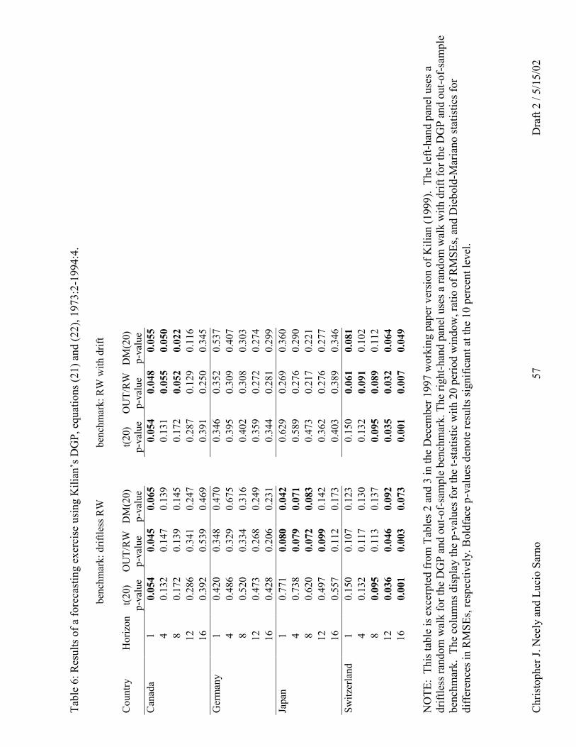
Chr
isto
pher
J. N
eely
and
Luc
io S
arno
D
raft
2 / 5
/15/
0257
Tabl
e 6:
Res
ults
of a
fore
cast
ing
exer
cise
usi
ng K
ilian
’s D
GP,
equ
atio
ns (2
1) a
nd (2
2), 1
973:
2-19
94:4
.
benc
hmar
k: d
riftle
ss R
Wbe
nchm
ark:
RW
with
drif
t
Cou
ntry
Hor
izon
t(20)
p-va
lue
OU
T/R
Wp-
valu
eD
M(2
0)p-
valu
et(2
0)p-
valu
eO
UT/
RW
p-va
lue
DM
(20)
p-va
lue
Can
ada
10.
054
0.04
50.
065
0.05
40.
048
0.05
54
0.13
20.
147
0.13
90.
131
0.05
50.
050
80.
172
0.13
90.
145
0.17
20.
052
0.02
212
0.28
60.
341
0.24
70.
287
0.12
90.
116
160.
392
0.53
90.
469
0.39
10.
250
0.34
5G
erm
any
10.
420
0.34
80.
470
0.34
60.
352
0.53
74
0.48
60.
329
0.67
50.
395
0.30
90.
407
80.
520
0.33
40.
316
0.40
20.
308
0.30
312
0.47
30.
268
0.24
90.
359
0.27
20.
274
160.
428
0.20
60.
231
0.34
40.
281
0.29
9Ja
pan
10.
771
0.08
00.
042
0.62
90.
269
0.36
04
0.73
80.
079
0.07
10.
589
0.27
60.
290
80.
620
0.07
20.
083
0.47
30.
217
0.22
112
0.49
70.
099
0.14
20.
362
0.27
60.
277
160.
557
0.11
20.
173
0.40
30.
389
0.34
6Sw
itzer
land
10.
150
0.10
70.
123
0.15
00.
061
0.08
14
0.13
20.
117
0.13
00.
132
0.09
10.
102
80.
095
0.11
30.
137
0.09
50.
089
0.11
212
0.03
60.
046
0.09
20.
035
0.03
20.
064
160.
001
0.00
30.
073
0.00
10.
007
0.04
9
NO
TE:
This
tabl
e is
exc
erpt
ed fr
om T
able
s 2 a
nd 3
in th
e D
ecem
ber 1
997
wor
king
pap
er v
ersi
on o
f Kili
an (1
999)
. Th
e le
ft-ha
nd p
anel
use
s adr
iftle
ss ra
ndom
wal
k fo
r the
DG
P an
d ou
t-of-
sam
ple
benc
hmar
k. T
he ri
ght-h
and
pane
l use
s a ra
ndom
wal
k w
ith d
rift f
or th
e D
GP
and
out-o
f-sa
mpl
ebe
nchm
ark.
The
col
umns
dis
play
the
p-va
lues
for t
he t-
stat
istic
with
20
perio
d w
indo
w, r
atio
of R
MSE
s, an
d D
iebo
ld-M
aria
no st
atis
tics f
ordi
ffer
ence
s in
RM
SEs,
resp
ectiv
ely.
Bol
dfac
e p-
valu
es d
enot
e re
sults
sign
ifica
nt a
t the
10
perc
ent l
evel
.
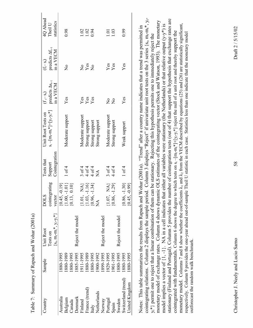
Chr
isto
pher
J. N
eely
and
Luc
io S
arno
D
raft
2 / 5
/15/
0258
Tabl
e 7:
Sum
mar
y of
Rap
ach
and
Woh
ar (2
001a
)
Cou
ntry
Sam
ple
Uni
t Roo
tTe
sts o
n{s
t, m
t-mt*
, yt-y
t*}
DO
LSco
inte
grat
ing
vect
or
Test
s tha
tSu
ppor
tC
oint
egra
tion
Uni
t Roo
t Tes
ts o
ns t
–[m
t-mt*
]+[y
t-yt*
](f
t– s t
)pr
edic
ts ∆
s t+1
in a
VEC
M
(ft–
s t)
pred
icts
∆f t+
1
in a
VEC
M
4Q A
head
Thei
l Ust
atis
tics
Aus
tralia
1880
-199
5{0
.45,
-0.1
9}B
elgi
um18
80-1
989
{1.0
0, -1
.01}
1 of
4M
oder
ate
supp
ort
Yes
No
0.98
Can
ada
1880
-199
5{0
.13,
0.1
0}D
enm
ark
1885
-199
5R
ejec
t the
mod
elFi
nlan
d19
11-1
995
{1.0
1,
NA
}3
of 4
Mod
erat
e su
ppor
tY
esN
o1.
02Fr
ance
(tre
nd)
1880
-198
9{1
.03,
-1.1
6}4
of 4
Stro
ng su
ppor
tY
esY
es1.
02Ita
ly18
80-1
995
{0.9
6, -1
.34}
4 of
4St
rong
supp
ort
Yes
No
0.94
Net
herla
nds
1900
-199
2N
AN
ASt
rong
supp
ort
Nor
way
1899
-199
5R
ejec
t the
mod
elPo
rtuga
l19
29-1
995
{1.0
7,
NA
}3
of 4
Mod
erat
e su
ppor
tN
oY
es1.
01Sp
ain
1901
-199
5{0
.86,
-1.2
9}4
of 4
Stro
ng su
ppor
tN
oY
es1.
03Sw
eden
1880
-199
5R
ejec
t the
mod
elSw
itzer
land
(tre
nd)
1880
-199
5{0
.86,
-1.3
0}1
of 4
Wea
k su
ppor
tY
esY
es0.
99U
nite
d K
ingd
om18
80-1
995
{0.4
5, -0
.99}
Not
es:
This
tabl
e su
mm
ariz
es th
e re
sults
from
Rap
ach
and
Woh
ar (2
001a
). “
Tren
d” a
fter a
cou
ntry
nam
e in
dica
tes t
hat a
tren
d w
as p
erm
itted
inco
inte
grat
ing
rela
tions
. C
olum
n 2
disp
lays
the
sam
ple
perio
d. C
olum
n 3
disp
lays
“R
ejec
t” if
uni
varia
te u
nit r
oot t
ests
on
the
3 se
ries {
s t, m
t-mt*
, yt-
y t*}
per
mit
one
to re
ject
that
a li
near
com
bina
tion
of th
em c
an b
e st
atio
nary
. R
ejec
ting
this
hyp
othe
sis p
erm
its o
ne to
imm
edia
tely
reje
ct th
em
onet
ary
mod
el o
f exc
hang
e ra
tes.
Col
umn
4 sh
ows d
ynam
ic O
LS e
stim
ates
of t
he c
oint
egra
ting
vect
or (S
tock
and
Wat
son,
199
3).
The
mon
etar
ym
odel
impl
ies a
vec
tor o
f {1,
-1}.
NA
in a
cel
l ind
icat
es th
at e
ither
all
varia
bles
wer
e st
atio
nary
(the
Net
herla
nds)
or t
hat r
elat
ive
outp
ut (y
-y*)
isst
atio
nary
(Fin
land
and
Por
tuga
l). C
olum
n 5
prov
ides
the
num
ber o
f coi
nteg
ratio
n te
sts (
out o
f 4) t
hat s
uppo
rt th
e hy
poth
esis
that
exc
hang
e ra
tes a
reco
inte
grat
ed w
ith fu
ndam
enta
ls. C
olum
n 6
show
s the
deg
ree
to w
hich
test
s on
s t –[
mt-m
t*]+
[yt-y
t*] r
ejec
t the
nul
l of a
uni
t roo
t and
ther
eby
supp
ort t
hem
onet
ary
mod
el.
Col
umns
7 a
nd 8
show
whe
ther
the
coef
ficie
nts λ
1 and
λ2 f
rom
the
VEC
M d
escr
ibed
by
equa
tions
(25)
and
(26)
are
stat
istic
ally
sign
ifica
nt,
resp
ectiv
ely.
Col
umn
9 pr
ovid
es th
e on
e-ye
ar a
head
out
-of-s
ampl
e Th
eil U
stat
istic
in e
ach
case
. St
atis
tics l
ess t
han
one
indi
cate
that
the
mon
etar
y m
odel
outfo
reca
st th
e ra
ndom
wal
k be
nchm
ark.