lecture notes 3 the monetary approach to flexible exchange ... · the monetary approach to flexible...

Lecture Notes 3

The Monetary Approach to Flexible

Exchange Rates

International Economics: Finance Professor: Alan G. Isaac

3 The Monetary Approach 1

3.1 Key Ingredients of the Monetary Approach . . . . . . . . . . . . . . . . . . . 2

3.1.1 Exogenous Real Exchange Rates . . . . . . . . . . . . . . . . . . . . . 3

3.1.2 The Classical Model of Price Determination . . . . . . . . . . . . . . 4

3.2 The Crude Monetary Approach Model . . . . . . . . . . . . . . . . . . . . . 6

3.2.1 Core Predictions . . . . . . . . . . . . . . . . . . . . . . . . . . . . . 7

3.2.2 Early Tests of the Monetary Approach Model . . . . . . . . . . . . . 12

3.2.3 Volatility Puzzle . . . . . . . . . . . . . . . . . . . . . . . . . . . . . 18

3.3 Exchange Rates and Monetary Policy . . . . . . . . . . . . . . . . . . . . . . 19

3.3.1 Money Supply Shocks . . . . . . . . . . . . . . . . . . . . . . . . . . 19

3.3.2 Money Growth Shocks . . . . . . . . . . . . . . . . . . . . . . . . . . 20

3.4 Transitory Shocks . . . . . . . . . . . . . . . . . . . . . . . . . . . . . . . . . 24

1

3.4.1 Money Supply Shock . . . . . . . . . . . . . . . . . . . . . . . . . . . 25

3.5 Anticipated Monetary Policy . . . . . . . . . . . . . . . . . . . . . . . . . . . 26

3.5.1 An Anticipated Change in the Money Supply . . . . . . . . . . . . . 26

3.5.2 An Anticipated Change in Money Growth . . . . . . . . . . . . . . . 29

3.6 Conclusion . . . . . . . . . . . . . . . . . . . . . . . . . . . . . . . . . . . . . 31

Terms and Concepts . . . . . . . . . . . . . . . . . . . . . . . . . . . . . . . 32

Problems for Review . . . . . . . . . . . . . . . . . . . . . . . . . . . . . . . 34

.1 Empirical Monetary Approach Models . . . . . . . . . . . . . . . . . . . . . 39

.1.1 Characterizing Money Demand . . . . . . . . . . . . . . . . . . . . . 39

.1.2 Testing the Monetary Approach . . . . . . . . . . . . . . . . . . . . . 41

.2 Partial Adjustment of Money Demand . . . . . . . . . . . . . . . . . . . . . 44

2 LECTURE NOTES 3. THE MONETARY APPROACH

This chapter is our first attempt to understand exchange rate determination. A good

model will help us understand the past and anticipate the future. In chapter 2 we saw that

many economic decisions are affected by expectations of future exchange rates. Yet exchange

rates are notoriously hard to predict. One way economists hope to improve our exchange

rate predictions is by discovering the fundamental determinants of exchange rate movements.

The monetary approach to flexible exchange rates focuses on domestic and foreign money

supply and money demand. Monetary policy is given the central role in exchange rate

determination. The determinants of domestic and foreign money demand also prove to be

fundamental determinants of the exchange rate.

3.1 Key Ingredients of the Monetary Approach

The monetary approach has two key ingredients: exogeneity of the real exchange rate, and

a simple Classical model of price level determination.1 Exogeneity of the real exchange rate

means that inflation at home or abroad will not affect how much foreign goods cost in terms

of domestic goods. The Classical model of price determination says roughly that the price

level is proportional to the money supply, so that monetary policy is the key determinant of

inflation rates.

Eventually, we will explore both of these constituents in some detail. Suffice it to say

that as short-run descriptions of real economies, both appear quite unrealistic. However as

long-run descriptions, they show somewhat more promise. So the monetary approach to

flexible exchange rates is best seen as a description of long-run outcomes. As a description

of short-run outcomes, it serves as a reference model that highlights some core concerns in

our attempt to understand exchange rate determination.

1Some authors treat uncovered interest parity as central to the monetary approach. We will not needthis restriction. We treat the risk premium as exogenous but possibly nonzero.

3.1. KEY INGREDIENTS OF THE MONETARY APPROACH 3

3.1.1 Exogenous Real Exchange Rates

Let P be the domestic consumer price index and P ∗ be the foreign consumer price index.

For now, we will keep things simple by thinking of each price index as the monetary cost of

a fixed consumption basket. Equation (3.1) defines the real exchange rate, Q.

Qdef=

SP ∗

P(3.1)

We call Q the real exchange rate because it tells you the rate at which domestic goods must

be given up to obtain foreign goods. The monetary approach to flexible exchange rates

assumes that Q is exogenous. This exogeneity assumption fits naturally with the Classical

model of price determination, which generally treats real variables as exogenous.

Given the real exchange rate, the nominal exchange rate and the relative price level have

a determinate relationship given by (3.2).

S = QP

P ∗(3.2)

Here S is the exchange rate, P is the domestic price index, P ∗ is the foreign price index,

and Q is the exogenous real exchange rate. For any given Q, equation (3.2) requires that ex-

change rate movements offset price level movements so that the rate at which goods actually

exchange for each other remains unchanged.

Purchasing Power Parity

Most presentations of the monetary approach to flexible exchange rates assume that the real

exchange rate is not only exogenous but that it is invariant. This is called the purchasing

power parity assumption.2 Constancy of the real exchange rate implies that the exchange

2Given a common base year and identical price index construction, the relative price level, P/P ∗, is oftencalled the purchasing power parity exchange rate (or sometimes simply the purchasing power parity). Seechapter 5 for a detailed discussion of purchasing power parity. You may simplify for now by setting Q = 1and thinking of PPP as an application of the law of one price.


rate is proportional to the relative price level. For example, suppose domestic inflation leads

to a doubling of the domestic prices, while foreign inflation is zero. Then a doubling of the

exchange rate will leave the real exchange rate unchanged. As a theory of exchange rate

determination, this is only a beginning: it does not explain the determination of relative

price levels.3 That is our next project.

3.1.2 The Classical Model of Price Determination

In the Classical model of price level determination, the supply of money determines the

(perfectly flexible) price level. In the simple Classical model, monetary policy has no influence

on real economic activity. The real interest rate and real income are determined in the goods

and labor markets independently of monetary policy. This dichotomy (i.e., independence of

the real sector from the monetary sector) is a helpful simplification when we model monetary

phenomena such as the nominal interest rate, the inflation rate, or the exchange rate. It

allows us to treat real income, the real interest rate, and even the real exchange rate as

exogenous when we are modeling the determination of the price level.

Four key assumptions of the simple Classical model are relevant to the determination of

the price level.

• real money demand (L) is a stable function of real income (Y ) and the nominal interest

rate (i).

• the money market is in continuous equilibrium.

• in addition to real income (Y ) and the real interest rate r, the nominal money supply

(H) is exogenous.

• the price level (P ), not the interest rate (i), moves to clear the money market.

3In fact some economists consider it less than a beginning, since they feel that the relevant price indices(P and P ∗) are not observable Hodrick (1978); MacDonald (1993).

3.1. KEY INGREDIENTS OF THE MONETARY APPROACH 5

The first two of these assumptions are common to almost all macroeconomic models. The

last two assumptions are specific to models in the Classical tradition.

The first assumption is implied by standard theoretical treatments of the demand for

money.4 It embodies the theoretical dependence of liquid transactions balances on the de-

sired level of transactions and the opportunity cost of liquidity. The nominal interest rate

represents the opportunity cost of holding money rather than less liquid assets, and real in-

come proxies the real value of monetized transactions in the economy. A rise in the interest

rate therefore decreases money demand, while a rise in real income increases money demand.

Our real money demand function can therefore be written as L(−i ,

+

Y ).

The second assumption is also standard to almost all macroeconomic models, and since

adjustments can take place very rapidly in asset markets, it is very reasonable. It says that

the real money supply is always equal to real money demand:

H

P= L(i, Y ) (3.3)

Equation (3.3) is a characterization of money market equilibrium, where H is the money

supply, P is the price level, i is the nominal interest rate, Y is real income, and L(·, ·) is

the real money demand function. So (3.3) says that real money supply equals real money

demand, where real money demand is a stable function of i and Y .

The third assumption lists the standard exogeneity assumptions of the simple Classical

model. For the moment we will additionally treat the nominal interest rate as exogenous—an

assumption we will soon drop. The final assumption, perfect price flexibility, is very strong.

It implies that our model of money market equilibrium can be interpreted as a model of

price level determination.

We are now ready to model our Classical theory of price determination. The theory states

that nominal money supplies and real money demand determine the price level. Specifically,

4In empirical work, however, this formulation is used for long-run real money demand. Short-run moneydemand functions are generally characterized in terms of a partial adjustment to the desired long-run level(?).


the price level is determined as the ratio of nominal money supply to real money demand,

where real money demand is determined by real income and the nominal interest rate.

Algebraically, we simply solve (3.3) for the price level, which gives us (3.4) a simple Classical

model of price determination.

P =H

L(i, Y )(3.4)

Basic Predictions of the Classical Model

Equation (3.3) suggests some immediate predictions of our simple Classical model of price

level determination. Given the interest rate, an exogenous increase in the money supply

raises the price level so as to leave the real money supply unchanged.5 This is the core

Classical story about price determination: changes in the money supply simply change the

price level proportionately without causing any real changes in the economy. Changes in

money demand also affect the price level, of course. An increase in real income raises real

money demand, and the price level falls to restore equilibrium. Similarly, an increase in the

interest rate lowers real money demand, and the price level rises to restore equilibrium.

3.2 The Crude Monetary Approach Model

The monetary approach applies our simple Classical Model to the determination of the price

level in both at home and abroad. The foreign country equivalent of (3.4) is (3.5).

P ∗ =H∗

L∗(i∗, Y ∗)(3.5)

Here an asterisk indicates a foreign value. In each county, the price level is determined by

the ratio of the nominal money supply to real money demand. It follows that the relative

price level is determined by the ratio of the relative nominal money supply to relative real

5Recall that the Classical Model treats H and Y as exogenous. Interest rate determination is consideredin section 3.3.2.

3.2. THE CRUDE MONETARY APPROACH MODEL 7

money demand.

P

P ∗=

H/H∗

L(i, Y )/L∗(i∗, Y ∗)(3.6)

This is true even if these two economies are completely closed. Our consideration of specifi-

cally open-economy considerations begins with the introduction of the exchange rate.

In the monetary approach, the exchange rate is determined directly by the relative price

level via purchasing power parity (PPP). We use (3.2) and (3.6) to write the crude monetary

approach model to exchange rate determination as (3.7).

S = QH/H∗

L(i, Y )/L∗(i∗, Y ∗)(3.7)

We call the model “crude” because it remains incomplete: we have not yet modeled the

determination of interest rates. Nevertheless, the crude monetary approach does express

the exchange rate in terms of variables for which data are readily available—interest rates,

incomes, and money supplies—and such data have been used to test it. (See section 3.2.2.)

These variables are often referred to as exchange rate fundamentals, and an implication of

the monetary approach is that these exchange rate fundamentals should help us explain and

predict the behavior of the exchange rate.

3.2.1 Core Predictions of the Monetary Approach to Flexible Ex-

change Rates

The core prediction of the monetary approach to exchange rate determination is that relative

money supplies affect the exchange rate. Looking at (3.7), we can see that an increase in

the relative money supply leads to a depreciation of the exchange rate.

↑ H/H∗ −→ ↑ S (3.8)


P/P ∗

S

6

-

LM LM′

��

��

��

��

��

��

��

��PPP

vE2

vE1

dP/P ∗

dS

Figure 3.1: Money Supply Increase

Since the monetary approach to exchange rate determination is based upon the purchasing

power parity relationship, this result is naturally expected. A change in the relative money

supply changes the exchange rate because it affects the relative price level. A higher relative

money supply implies a higher relative price level, and by PPP the exchange rate changes

with the relative price level.

The prediction is even more specific than this. If the relative money supply doubles,

so does the relative price level If the relative price level doubles, so does the spot rate. So

according to the monetary approach to flexible exchange rates, the movement in the spot rate

is proportional to the movement in the relative money supply. That is, for each percentage

change in the relative money supply, there is a one percent change in the spot rate. We say

that the elasticity of the spot rate with respect to the relative money supply is unity.

Symmetrically, an increase in relative money demand leads to an appreciation of the

exchange rate.

↑ L/L∗ −→ ↓ S (3.9)

Once again, this is simply a reflection of the effects of relative money demand on the relative

price level. We know that a rise in Y or a fall in i will raise domestic money demand,

which increases relative money demand. So the monetary approach predicts that a rise in


domestic income or a fall in the domestic interest rate will appreciate the domestic currency.

Symmetrically, a rise in Y ∗ or a fall in i∗ will raise foreign money demand, which decreases

relative money demand. So the monetary approach predicts that a rise in foreign income or

a fall in the foreign interest rate will depreciate the domestic currency.

Of course money demand can change for other reasons, such as deregulation and finan-

cial innovation. (As examples of innovation, think of the spread of credit cards or ATM

machines.) Many observers believe that such factors destabilized money demand in the

1980s and 1990s. The monetary approach predicts that financial innovation that reduces the

demand for money will cause the domestic currency to depreciate.

The exchange rate is the domestic currency price of foreign money, so it is natural that an

increase in the supply of foreign money will appreciate the domestic currency (i.e., lower the

price of foreign exchange) while an increase in the demand for foreign money will depreciate

the domestic currency (i.e., increase the price of foreign exchange). This is just what happens

in the monetary approach.

1% Increase In: H H∗ Y Y ∗ i i∗

Resulting ∆S: 1% -1% – + + –

Table 3.1: Core Predictions: Crude Monetary Approach

Inflation in Zaire

We have seen that a core prediction of the monetary approach to flexible exchange rates is

that, ceteris paribus, money supply increases cause inflation and corresponding depreciation.

Even though other factors are always changing, this theory would certainly predict that

very large, sustained increases in the money supply will produce inflation and associated

currency depreciation. This makes the experience of high inflation countries relevant to a

first assessment of the monetary approach. In particular, hyperinflations seem to offer natural

testing grounds for the monetary approach model. After all, one of its core components is

the Classical model of price determination. which emphasizes long-run relationships between


the money supply and other nominal variables (such as prices or exchange rates). In a

hyperinflation, changes in such nominal variables dwarf all the real changes in the economy.

We might therefore hope that, during a hyperinflation, the kinds of relationships emphasized

by the Classical model would be more readily exposed to view.

Consider the example of Zaire. In the mid-1990s, Zaire experienced an unusually long

and severe hyperinflation. During the late 1980s the country had experienced high inflation,

around 70% per year. At the end of 1990, things took a turn for the worse. Haughton (1998)

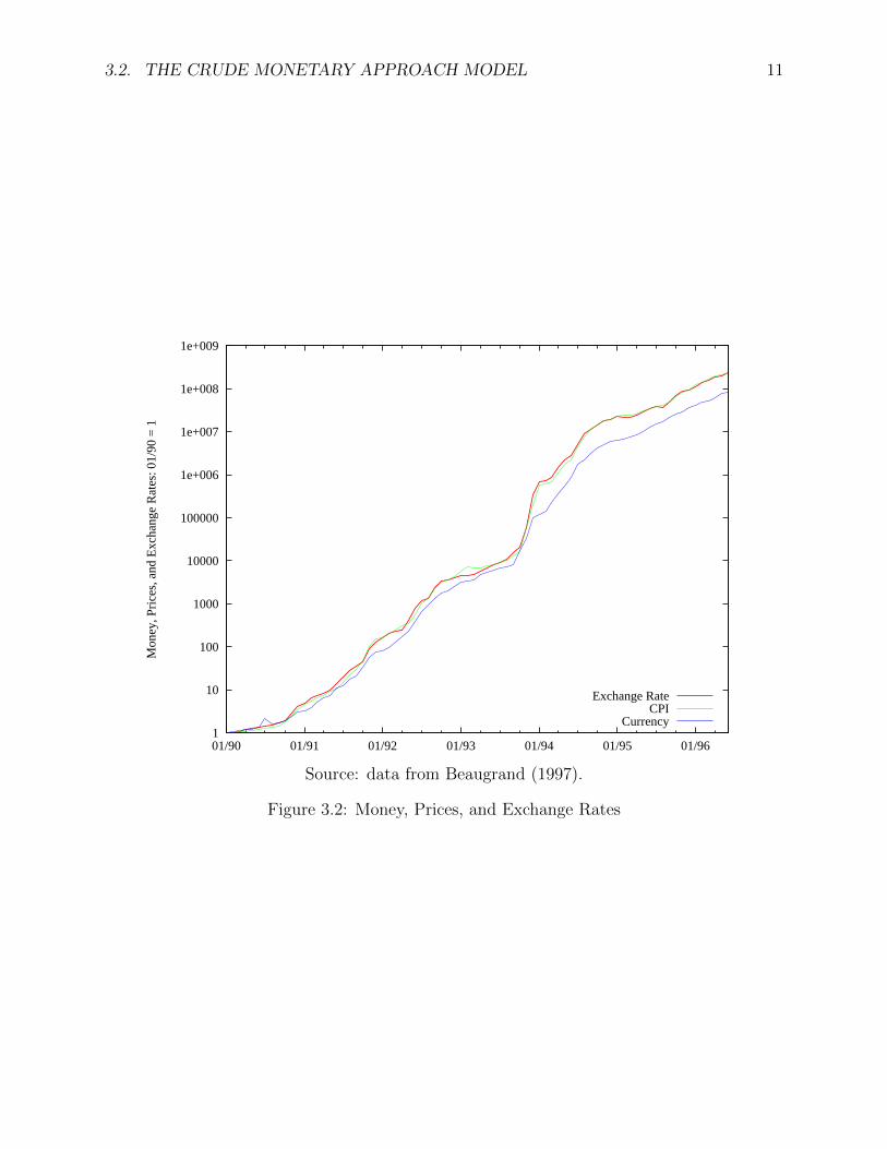
reports that in five years consumer prices rose a total of 6.3 billion percent. Beaugrand (1997)

reports inflation of nearly 10,000% in 1994. In the midst of all this was a failed currency

reform in 1993. On October 22, 1993, at the rate of one for every 3 million (old) zaire, and

was initially fixed at 3nz/$ (Beaugrand, 1997).6 By 1997, a 1-million-zaire note was worth

about $3 in Kinshasa. Figure 3.2 illustrates the simultaneous inflation and depreciation, as

predicted by the monetary approach to flexible exchange rates.

Inflation in Zimbabwe

Between early 2006 and early 2007, prices in Zimbabwe rose by more than 1,000%.

The Mugabe government nevertheless refused to devalue the Zimbabwean dollar, which

on the black market was worth only 5% of its official value. Gideon Gono, governor of the

Reserve Bank, announced plans to reduce broad money supply growth from ”over 1,000

percent to between 415 and 500 percent by December 2007 and subsequently to under 65

percent by December 2008.” While this showed a good awareness of the source of inflation,

the next month Gono offered a change in policy that was parodic: he announced that price

increases would be illegal from March through June. This policy was abandoned when

shortages quickly emerged. In July 2008, Gono estimated the inflation rate at 2.2 million

percent and was immediately challenged by analysts who calculated it at more that 12 million

percent. By one report, a loaf of bread rose in price from a billion Zimbabwean dollars to 100

6In an interesting aside (Haughton, 1998) reports: “The new notes were not accepted by residents ofKasai province, who continue to use only the old notes; inflation in the province is said to be negligible.”


1

10

100

1000

10000

100000

1e+006

1e+007

1e+008

1e+009

01/90 01/91 01/92 01/93 01/94 01/95 01/96

Mon

ey, P

rice

s, a

nd E

xcha

nge

Rat

es: 0

1/90

= 1

Exchange RateCPI

Currency

Source: data from Beaugrand (1997).

Figure 3.2: Money, Prices, and Exchange Rates


billion in about a day. The new 100 billion dollar note issued in mid-July was not enough to

buy a loaf of bread by the end of July. Dollarization, although illegal, became increasingly

common.

3.2.2 Early Tests of the Monetary Approach Model

Naturally economists wish to determine the extent to which the available data are supportive

of the core predictions of their models. Before we can develop specific tests of the monetary

approach to flexible exchange rates, we need to find data that appropriately represent the

variables in our model. We must also parameterize relationships that we have been describing

only in the most general terms, perhaps by specifying a functional form for the money demand

function. So before proceeding to the empirical test of the monetary approach, we need to

discuss relative real money demand in a bit more detail.

We have been writing our money demand functions as L(i, Y ) and L∗(i∗, Y ∗). This

represents in a general fashion our assumption that money demand is a stable function of

the nominal interest rate and real income. Monetary theory tells us that real money demand

responds positively to real income, which is a proxy for the level of transactions in the

economy, and negatively to the interest rate, which is a proxy for the opportunity cost of

holding money. The monetary approach to flexible exchange rates tells us that these money

demand responses are also relevant to exchange rate determination: the spot rate responds

negatively to real income, due to the implied rise in money demand, and negatively to the

interest rate, due to the implied fall in money demand. When we conduct an econometric

investigation of the monetary approach to flexible exchange rates, we let the data suggest

numerical values for the sizes of these responses. For example, we estimate the elasticity of

the spot rate with respect to real income. We would like to learn whether our theoretical

predictions match the relationships present in the data. We are therefore interested in the

sign and the size of our estimates.

Table 3.2 lists some of the early econometric tests of the monetary approach to flexible


exchange rates. The first study in the list is by far the most famous: Jacob Frenkel’s study of

the post-WWI German hyperinflation. As we have discussed, since nominal changes dwarf

real changes during a hyperinflation, we might hope that the kinds relationship between

money and exchange rates stressed by the monetary approach will be more readily detected

in the data. In the case of the German hyperinflation, Frenkel felt this justified ignoring

changes in domestic income and all foreign variables, since the changes in these variables

were very small compared to the huge changes in the spot rate and German money supply

that took place during the hyperinflation. He estimated the response of the spot rate to only

two variables: the German money supply, and the opportunity cost of money.

Estimated Response of the Spot Rate to:Study: Sample: H H∗ Y Y ∗ i i∗

DEM/GBP

Frenkel (1976) 1921.02–1923.08 0.975 – – – 0.591 ←Bilson (1978b) 1972.01–1976.04 1.0013 -1.0081 -1.0184 0.9990 0.0228 ←Bilson (1978a) 1970.04–1977.05 1.0026 -0.9846 -0.9009 1.0183 1.3853 ←

USD/DEM

Hodrick (1978) 1973.04–1975.09 1.52 -1.39 -2.23 0.073 2.53 1.93GBP/USD

P&W (1979) 1972–1977 0.63 ← -0.77 ← 0.14 ←Note: The reported “responses” are money supply elasticities, income elasticities, and opportunity-cost semi-elasticities of the spot rate. Opportunity costs of holding money are proxied by interest rates or forwarddiscounts. A dash indicates an omitted variable. A left arrow indicates that the domestic and foreign moneydemand parameters are constrained to equality.

Table 3.2: Early Tests of the Monetary Approach

Frenkel’s results are summarized in table 3.2. The dashes indicate responses that he

did not estimate, and the left arrow indicates that he constrained to equality the response

to the domestic and foreign interest rate.7 His estimates, using monthly German data, are

correctly signed, significantly different from zero, and of plausible magnitude. In addition,

money supply elasticity of the spot rate differs insignificantly from unity. Many economists

viewed Frenkel’s results as providing dramatic support for the monetary approach.

Bilson (1978a; 1978b) offers additional early evidence on the crude monetary approach

model. Bilson (1978b) estimated a model of the DEM/GBP exchange rate using monthly

7We discuss his opportunity cost measure in more detail below.


data for the period 1972.01–1976.04. The results are reported in table 5.8 Overall the

results look fairly good. However the coefficient on his opportunity cost measure is not

statistically different from zero, and Bilson required considerable econometric manipulation

to arrive at the reported results. The study therefore lends modest support to the crude

monetary approach. Bilson (1978a) extends this sample to 1970.04–1977.05. (Note that this

includes some years preceding the general float.) After resorting to a complicated estimation

procedure, Bilson finds the results reported in table 5.9 His estimates have the correct sign

and reasonable magnitude. All the coefficients are significantly different from zero. Again

the coefficients on money supplies are close to unity, the value implied by the monetary

approach.

Keep in mind that flexible prices, PPP, and stable money demand lie at the core of the

monetary approach. It is therefore rather surprising, in a non-hyperinflationary setting, that

the monetary approach performed so well with monthly data. Price flexibility and PPP are

most likely to hold in the longer run. Indeed, as we shall see, PPP performs very poorly

in the short run, and an important reason appears to be price stickiness. Furthermore, the

assumption of a stable money-demand function has become increasingly suspect during the

post-Bretton Woods era (?).

Hodrick (1978) and Putnam and Woodbury (1979–80) also offer early empirical tests

of (3.7) using monthly data from developed countries. Hodrick (1978, eq.7) examine the

USD/DEM exchange rate from April 1973 to September 1975. The first row of table 3.1

reports his estimated reponses of the spot rate to money, interest rates, and income.10

Recall that theory predicts that the spot rate moves proportionally to the relative money

supply, or equivalently that it is unit elastic with respect to the relative money supply. In

8The reported results are for his equation (45), which reports long-run coefficients calculated from an es-timation incorporating a partial adjustment money demand equation. (See problem 8.) He also incorporatesprior expectations about the coefficients in his estimation procedure.

9This is his equation (12). Not reported in the table is his coefficient on a time trend, which suggests ahalf a percent appreciation of the DEM per month. This adds up: over the period, it makes an importantcontribution to the model’s predicted values.

10See Hodrick’s article for a discussion of the data and of his variable definitions.


table 3.2, we therefore would hope to find numbers close to 1 in the H column and close

to -1 in the H∗ column. While we do not find a perfect match, the estimated responses

were close enough for Hodrick to conclude that the data did not reject this prediction of the

monetary approach. His results are somewhat favorable to the theory, in the sense that his

estimated responses generally have the predicted signs, are significantly different than zero,

and are of plausible magnitude. Moreover, he reports that exchange rate fundamentals are

explaining about two-thirds of the variation in the spot rate. Nevertheless, there are a couple

of noticeable problems. German income appears to have a weak influence on the exchange

rate. (The response is smaller than expected; in fact, Hodrick finds that it is insignificantly

different from zero.) Worse, the spot rate response to the German interest rate is the wrong

sign (and differs significantly from zero).11 The support for the flexprice monetary approach

model offered by Hodrick’s research is modest at best.

Putnam and Woodbury’s results are somewhat more encouraging. Their estimates are

also reported in Table 3.2.12 They use data from 1972–77 to examine the GBP/USD ex-

change rate. Table 3.2 reports their results for monthly data; they also report results for

quarterly data, which look similar. Fewer coefficients are reported because they reported

results when relative money, relative income, and the relative interest rate are the regres-

sors, thus constraining the domestic and foreign responses to be the same. (They report

that relaxing these constraints produces comparable results.) All the coefficients have the

correct sign and are significantly different from zero. The coefficient on relative income is

disappointingly far from its predicted value of zero, but the regression otherwise provides

good support for the monetary approach to flexible exchange rates.

11Hodrick suggests that German capital controls adopted in February 1973 might offer an explanation,but in the context of the monetary approach this is not evident.

12The estimated “responses” are money supply elasticities, income elasticities, and interest rate elasticitiesof the spot rate. They have corrected for first order autocorrelation with a Hildreth-Lu procedure. See theirarticle for a discussion of the data and for variable definitions.


Using the Forward Discount

When we begin to think about empirical applications of the monetary approach, we have

to decide what measured quantities will represent each of the variables in our exchange

rate equation (3.7). For example, there are many different foreign and domestic interest

rates: which are appropriate for our purposes? Rather than choose an interest rate, some

researchers have turned to the forward discount on domestic currency.

Use of the forward discount instead of domestic and foreign interest rates requires a

special assumption, which is fairly standard in the empirical literature testing the monetary

approach to flexible exchange rates. This is the assumption of a common interest rate

response in foreign and domestic money demand. Relative real money demand is given a

special form:

L(i, Y )/L∗(i∗, Y ∗) = L(i− i∗, Y, Y ∗) (3.10)

With this assumption, we can write

S = QH/H∗

L(i− i∗, Y, Y ∗)(3.11)

In this version of the crude monetary approach, the foreign and domestic interest rates enter

only as an interest rate differential (i − i∗). Recall that chapter 2 developed the covered

interest parity condition.

fd = i− i∗ (3.12)

With high capital mobility, covered interest parity should hold closely for assets that are

good substitutes. So one natural way to measure the interest rate differential in the monetary

approach model is with the forward discount. This yields (3.13).

S = QH/H∗

L(fd , Y, Y ∗)(3.13)


Frenkel (1976) used this approach in his study of the post-WWI German hyperinflation.13

Bilson 1978a; 1978b also uses the forward discount to proxy the relative opportunity costs

of holding domestic and foreign money.

In-Sample Fit and Out-of-Sample Forecasting

Later studies proved less supportive of the crude monetary approach to flexible exchange

rates. It turns out that the in-sample fit of monetary approach models depends on the choice

of exchange rate and the sample period. This is rather discouraging news. In addition, only

a small fraction of the actual variation in the exchange rate is explained by the monetary

approach model. However in-sample fit is only one criterion for model performance, and

arguably it is not the most interesting criterion. Since the mid-1980s, economists have been

more interested in evidence of the predictive power of their models. In particular, exchange

rate research has concentrated on the out-of-sample forecasting ability of existing models.

A model that is capable of improving our exchange rate forecasts can be very useful even if

its in-sample fit is disappointing.

The classic study of the out-of-sample forecasting ability of modern exchange rate models

is Meese and Rogoff (1983). Meese and Rogoff pit a one-step-ahead random-walk model

against the core inflation and other models. Using monthly data (1973.03-1981.06) for several

countries, they found that the one-step-ahead random walk model outperforms the structural

models in forecasting the exchange rate. However Schinasi and Swamy (1987) argue that

the one step ahead forecasts favor the random walk model, which uses the lagged exchange

rate. They find much greater forecast error in the multi-step random walk forecasts. And

indeed, adding a lagged dependent variable to the structural models greatly improves their

forecasting performance.14

13Frenkel’s justification of using the forward discount was somewhat different than that offered here.14Other studies finding some advantages from including the lagged spot rate include Woo (1985), Somanath

(1986), Boughton (1987), Driskill et al. (1992), and MacDonald and Taylor (1994).


3.2.3 Volatility Puzzle

Recall that the crude monetary approach to flexible exchange rates, as represented by (3.7),

explains the exchange rate in terms of a small number of exchange rate fundamentals: inter-

est rates, incomes, and money supplies. Although we expect short-run deviations from this

relationship, we might hope that such deviations are not large relative to the volatility of the

exchange rate. However the exchange rate is surprisingly volatile relative to these fundamen-

tals. In order to highlight this volatility puzzle for the monetary approach, Flood and Rose

(1999) aggregate these fundamentals in order to offer a rough comparison of the variability

of the exchange rate and the variability of the fundamentals.15 Two problems emerge. First,

for the 1980s and 1990s Flood and Rose (1999) find no link across countries between the

volatility of aggregate fundamentals and exchange-rate volatility. Second, they can find no

evidence that countries tend to experience periods of volatile exchange rates at the same

time as they experience volatility in the aggregate fundamentals. For example, the collapse

of the Bretton Woods system of pegged exchange rates produced a tremendous increase in

exchange-rate volatility without noticeably increasing the volatility of the aggregate funda-

mentals. To explain this, it seems we need to discover a new exchange rate fundamental that

behaves entirely differently under pegged and floating exchange-rate regimes.

15In addition to identical interest rate semi-elasticities, much empirical work assumes identical incomeelasticities as well. Constraining these to unity yields the Flood and Rose (1999) aggregate measure ofexchange rate fundamentals. Relative money demand becomes

L(i, Y )/L(i∗, Y ∗) = L(i− i∗, Y/Y ∗)

=Y/Y ∗

exp i− i∗

and the aggregate fundamentals are therefore

M/M∗

Y/Y ∗ exp i− i∗ (3.14)

3.3. EXCHANGE RATES AND MONETARY POLICY 19

3.3 Exchange Rates and Monetary Policy

It should be clear at this point that a basic contention of the monetary approach is that

monetary policy is an important determinant of the behavior of the exchange rate. We might

represent a change in monetary policy by a change in the level of the money supply or by a

change in its growth rate. This suggests two monetary policy “thought experiments” we can

consider in order to explore the basic predictions of the monetary approach.

3.3.1 Money Supply Shocks

An unanticipated exogenous disturbance of the economy is called a shock. Our first thought

experiment concerns a money supply shock: a one-time, permanent, unanticipated increase

in the domestic money supply, with no associated change in the expected growth rate of

the money supply over time. Keeping in mind this is a Classical style model, we expect the

domestic price level to increase proportionally (so that the real money supply is unchanged).

Keeping in mind the purchasing power parity condition, the exchange rate must increase

in proportion to the price level. So the model predicts a depreciation of the exchange rate

proportional to the increase in the money supply. This is easily seen in equation (3.7): if we

double H on the right hand side, we must double S on the left hand side to maintain the

equality.

The behavior of the money supply, the real money supply, the price level, and the spot

rate are illustrated in figure 3.3.16 The rise in the nominal money supply, H, takes place at

time t0. The change in the spot rate and the price level proportional to the change in the

nominal money supply, so the real money supply remains unchanged.

This first thought experiment illustrates what would happen in a Classical economy where

the money supply followed a “random walk”. This is the situation when each month the

money supply is just as likely to rise as to fall. Suppose you are asked to offer a single number

16Absolute heights are meaningless in the graphs: only relative changes matter. To keep the presentationas simply as possible, we have plotted P and S in the same graph. (This may be seen as a harmlessnormalization, where Q = 1 and P ∗ = 1.)


tt0

H

0 tt0

P,S

0 tt0

H/P

0

Figure 3.3: Increase H at t0

as your forecast of the next month’s money supply in such circumstances. To be as right

as possible on average, you should predict that the money supply will remain at its present

level. Next month you will be in the same position. The money supply may be higher or

lower than you had expected, but you should predict that it will stay at its new level. In

this sense, changes in the level of the money supply are permanent. However, changes in

the growth rate of the money supply tell us nothing about the future money supply growth

rate, which is always expected to be zero.17

3.3.2 Money Growth Shocks

The next experiment we want to consider is a one-time, permanent, unanticipated change in

the growth rate of the money supply. As a preliminary, we need to think a bit more carefully

about the role of interest rates in the monetary approach model.

Interest Rates and Inflation

The Classical model of interest rate determination begins with the following definition of the

real interest rate.

rdef= i− πe (3.15)

The real interest rate is the expected real rate of return from holding an interest bearing

asset. In an inflationary environment, part of the nominal rate of return on an asset simply

compensates for rises in the price level. For example, if an individual holds his wealth in

17Nothing is changed if the expected growth rate is some other constant, say 0.5%/month, except that wemust include this expected growth in our forecasts.


assets paying 10% per year when inflation is 10% per year, then the nominal interest rate

of 10% per year simply maintains the purchasing power of wealth but does not augment

it. The Classical model treats the real interest rate as exogenous, which turns (3.15) into a

theory of interest rate determination.

i = r + πe (3.16)

Equation (3.16) is often called the Fisher equation. It decomposes the nominal interest

rate into the real interest rate r and expected inflation πe. Since the real interest rate is

exogenous in the Classical model, variations in expected inflation imply variations in the

nominal interest rate. We can use the Fisher equation (3.16) to substitute for the nominal

interest rate in our representation of money market equilibrium (3.3). The result is (3.17).

H

P= L(r + πe, Y ) (3.17)

The representation of money market equilibrium in equation (3.17) predicts a decline in real

balances when expected inflation is higher. Expected inflation should be high when actual

inflation is persistently high, this is a prediction that we should be able to roughly test

simply by looking at real money balances in high inflation economies. Consider table 3.3,

which is based on data from several hyperinflations. The dates are the first and last months

for which the inflation rate exceeded 50%/month. The inflation rates in the third column

are the average monthly inflation rates for the period. The final column shows the smallest

level of real balances reached during the hyperinflation as a ratio of the level of real balances

held at the beginning of the hyperinflation. Despite tremendous growth in the money supply

during these hyperinflations, the real money supply is declining. High inflation raises the

expected cost of holding money. The table shows that the decline in real balances during

hyperinflations is dramatic, which supports the prediction of equation (3.17).


Country Dates %∆P/month (H/P )min/(H/P )0

Austria 1921.10–1922.08 47 0.350Germany 1922.08–1923.11 322 0.030Greece 1943.11–1944.11 365 0.007Hungary 1923.03–1924.02 46 0.390Hungary 1945.08–1946.07 19,800 0.003Poland 1923.01–1924.01 81 0.340Russia 1921.12–1924.01 57 0.270Source: McCallum (1989, p.135), based on data in Cagan (1956).

Table 3.3: Inflation and Real Money Demand

Additional Predictions of the Monetary Approach

While monetary policy is sometimes characterized in terms of changes in terms of changes in

the level of the money supply, it is more often characterized in terms of the rate of growth of

the money supply. Our next thought experiment determines the predictions of the monetary

approach for changes in money supply growth rates.

The simplest case to consider is a one-time, permanent increase in the rate of growth of

the money supply. Suppose such a change takes place today. Given our previous work on

the monetary approach to flexible exchange rates, we might expect that the rate of inflation

immediately adjusts to the new growth rate of the money supply, and that by purchasing

power parity this becomes the new rate of depreciation as well. This is basically correct, but

there must be an additional one time adjustment of the price level. This is because a higher

inflation rate implies a higher nominal interest rate, which lowers real money demand.

Recall the Fisher equation for the domestic interest rate.

i = r + πe

Similarly, the foreign interest rate can be written as

i∗ = r∗ + π∗e


Substituting for the nominal interest rates in (3.7) allows us to write our exchange rate

determination equation as (3.18).

S = QH/H∗

L(r + πe, Y )/L∗(r∗ + π∗e, Y ∗)(3.18)

Equation (3.18) is known as the core-inflation formulation of the monetary approach to

exchange rate determination because it focuses attention on the determinants of expected

inflation. This equation is particularly useful for developing the more detailed predictions of

the monetary approach to flexible exchange rates.

Too see this, apply (3.18) to our monetary policy experiment. Looking at (3.18), it

is clear that unless we say something specific about the behavior of expectations, we will

have little to say about the behavior of the exchange rate. Let expectations adjust very

quickly to the policy change. For any level of inflation expectations, we know from our

previous monetary policy experiment that the price level must rise proportionately to the

money supply increases. It is therefore natural to set expected as well as actual inflation

equal to the new money supply growth rate. The higher expected inflation rate lowers

domestic money demand. Prices must rise not only because the money supply is increasing

but also because real money demand has fallen. Thus we have a brief magnification effect :

the inflation rate measured over a period near the time of the policy change will actually

exceed the new money supply growth rate. Since exchange rate movements are determined

by purchasing power parity, the rate of depreciation must display a similar magnification

effect (Frenkel, 1976).

tt0

H

0 tt00

P ,S

tt0

H/P

0

Figure 3.4: Increase H at t0


Figure 3.4 illustrates these outcomes. The change in the money supply growth rate takes

place at time t0. We plot the time path of the growth rate of the money supply (H), the rate

of inflation (P ), and the rate of depreciation (S). We also graph the level of real balances

over time. Note that although the level of the money supply does not jump, the spot rate

and price level do jump. This jump is the source of the “magnification effect”. In contrast

with our previous experiment, the real money supply is changed by this experiment. This

change derives from the higher interest rate implied by higher expected inflation, which in

turn is a result of the change in monetary policy.

3.4 Transitory Shocks

We now consider how the exchange rate responds to transitory shocks, by which we will

mean exogenous changes that last for a single period.

Recall that our monetary approach model consists of two key ingredients: purchasing

power parity, and the Classical model of price determination.

S = QP/P ∗ (3.19)

P/P ∗ =H/H∗

L(3.20)

We have been working with a very simple model of money demand, where L depends on the

interest differential and relative income.

L = L(i− i∗, Y/Y ∗) (3.21)

In turn, we recognized that covered interest parity holds under perfect capital mobility, so

that

i− i∗ = fd = ∆se + rp (3.22)

3.4. TRANSITORY SHOCKS 25

So our model of the spot rate involves relative money demand, which depends on expected

depreciation. This suggests that any discussion of transitory shocks will require careful

attention to the role of expectations. In this section, our approach will be to treat individuals

as understanding that they are dealing with a transitory shock, which allows them to form

correct expectations about the future. Since individuals know that the exchange-rate will

return to its long-run equilibrium level next period, we have

∆se = (S+1 − S)/S = (S − S)/S (3.23)

This must affect our description of short run equilibrium in the money market, since we

must allow for the effects of interest rates on money demand, and in the short run interest

rates must move with the spot rate. The relative price level is now determined as

P/P ∗ =H/H∗

L(S−SS

+ rp, Y/Y ∗) (3.24)

and therefore must be negatively related to the current spot rate. This manifests as down-

ward slope to the LM curve, which we label LMsr to emphasize its dependence on the given

level of S.

Our monetary approach model to temporary shocks is therefore

S = QH/H∗

L(S−SS

+ rp, Y/Y ∗) (3.25)

3.4.1 Money Supply Shock

Suppose that the economy is initially in a long-run equilibrium, with spot rate S, when it

receives an unanticipated transitory shock to level of money supply. Since individuals know

that the exchange-rate will return to its long-run equilibrium level next period, we have

∆se = (S+1 − S)/S = (S − S)/S (3.26)


P/P ∗

S

6

-

@@@@@@@@@@@@@@

LMsr

@@@@@@@@@@@@@@

LM ′sr

��

��

��

��

��

��

��

��PPP

svEsrv

Elr

dP/P ∗

dS

S

Figure 3.5: Transitory Money Supply Increase

As with a permanent shock, the domestic currency must depreciate in response to the increase

in H. But individuals anticipate that there will be a subsequent appreciation, which lowers

the interest differential and increases the relative demand for money. This moderates the

short-run movement of the exchange rate, which is therefore less than in the case of a

permanent shock.

3.5 Anticipated Monetary Policy

In section 3.3 we considered two changes in monetary policy: a change in the level of the

money supply, and a change in its growth rate. In both cases we considered an unantici-

pated change in policy. We now consider what happens when these changes in policy are

anticipated.

3.5.1 An Anticipated Change in the Money Supply

Consider a one-time, permanent, anticipated increase in the level of the money supply. The

behavior of the money supply is identical to the first monetary policy experiment we con-

sidered in section 3.3. However, the increase in the money supply at time t0 is now known

at the earlier time ta. That is, at time ta we correctly anticipate an increase in the money

3.5. ANTICIPATED MONETARY POLICY 27

supply, which will take place at time t0.

Since the behavior of the money supply is identical to our earlier experiment with an

unanticipated change in the money supply, we might think that prices, exchange rates, and

real balances should also behave in the same fashion. And indeed, if expected inflation were

unaffected by the anticipated increase in the money supply—for example, if expectations were

“static” in the sense of being exogenously fixed—the outcomes would in fact be identical. But

when the increase in the money supply is anticipated, it is not plausible to treat expectations

as static.

When we expect the money supply to increase, we predict an increase in the price level.

This must show up immediately in the nominal interest rate, which is the real interest rate

plus expected inflation. The rise in the nominal interest rate decreases money demand, and

this in turn increases the equilibrium price level. By the purchasing power parity relation-

ship, the increase in the domestic price level shows up as a proportional depreciation of

the exchange rate. So an anticipated future money supply increase leads to inflation and

depreciation today. This is true no matter how far in the future is the anticipated change,

although the farther away it is the smaller today’s response will be.

tt0ta

H

0 tt0ta

P,S

0 tt0ta

HP

0

Figure 3.6: Anticipated Increase in H

Figure 3.6 characterizes the outcomes when we anticipate at time ta the increase in the

level of the money supply that does not take place until time t0. We can easily charac-

terize economic outcomes before ta and after t0. Before ta there is no expected inflation,

corresponding to the constant money supply. In line with this, actual inflation is zero, as is

exchange rate depreciation. After t0 expected inflation will be correct if it again matches the

zero money supply growth rate. So after t0 we should have expected inflation, actual infla-


tion, and exchange rate depreciation each at 0% per year. The difficulty lies in determining

what happens between ta, the time the policy is anticipated, and t0, the time the policy is

implemented.

Expectations play a critical role between ta and t0. To aid us in working through the eco-

nomic outcomes during this period, we will work with expectations that are very accurate:

the actual and anticipated economic outcomes are the same. One crucial key to understand-

ing the outcomes lies in the recognition that there cannot be any anticipated jumps in the

price level.

Here is why. Suppose you expected an upward jump in the price level next Friday. This

jump will lower the value of any money balances you are holding, so you would like to get

rid of your money balances the day before. But so would everyone else, and knowing this

you expect money demand to fall on Thursday, with the implication that you must expect

the jump in the price level to take place on Thursday instead of Friday. Of course you face

the same difficulty in expecting the price level to jump on Thursday. Or Wednesday. Or

any future day. The conclusion is that if there is to be a jump in the price level, it must be

unanticipated. So any jump in the price level must take place at ta, as soon as the policy

change is anticipated.

One implication of this analysis is that, in the case of anticipated changes in the money

supply, the contemporaneous link between expected inflation and expected changes in the

money supply is broken. Consider price determination in the Classical model, solving (3.17)

for (3.27). A rise in expected inflation causes an immediate jump in the price level and the

exchange rate.

P =H

L(r + πe, Y )(3.27)

Now we have enough information to predict the economic outcomes between ta and t0.

At ta, the price level rises. Since the money supply has not yet changed, this determines

an initial fall in real balances. The lower real balances are compatible with money market

equilibrium because of the increase in expected inflation. Remember, expected inflation

3.5. ANTICIPATED MONETARY POLICY 29

tracks actual inflation. But since the money supply has not yet increased, the rise in prices

implies a fall in real balances. Inflation expectations must rise over time so as to maintain

money market equilibrium at the falling level of real balances. Until the money supply

actually increases, the price level and the exchange rate keep rising. Correspondingly, real

balances keep falling.

In the middle graph you can see the changes in the price level: the actual inflation. In the

last graph, you can see the changes in real balances, which are due to changes in expected

inflation. Since actual and expected inflation are tied together by our assumption that

individuals form very accurated expectations, we need the inflation implied by the middle

graph to be consistent with the expected inflation implied by the last graph.

If individuals are very good at predicting the money supply increase, prices should have

risen just enough by the time of this increase that no further changes are necessary to restore

equilibrium in the money market. That is, the total change in the price level over the period

ta to t0 will be just proportional to the increase in the money supply that takes place at

time t0. At this new price level, the increased money supply is just adequate to raise real

balances back to their old level, which is the equilibrium level of real balances when expected

inflation is zero.

3.5.2 An Anticipated Change in Money Growth

In section 3.3.2, we characterized changes in monetary policy in terms of the rate of growth of

the money supply. Our final monetary policy thought experiment determines the predictions

of the monetary approach for anticipated changes in money supply growth rates.

Suppose at time ta we correctly anticipate a one-time, permanent, increase in the rate of

growth of the money supply, which will take place at time t0. Suppose annual money growth

will rise from zero to ten per cent. Once again, the price level and the inflation rate must

respond immediately to our expectations of a future policy change. Correspondingly, via the

purchasing power parity condition, the exchange rate also responds. Recall that increases


in expected inflation immediately increase the exchange rate (by reducing relative money

demand and thereby increasing the relative price level).

In figure 3.7, we can once again easily characterize economic outcomes before ta and

after t0. Before ta there is constant expected inflation, corresponding to the constant money

supply growth rate. Let us say this growth rate is 5% per year. In line with this, actual

inflation is 5% per year, as is exchange rate depreciation. After t0 expected inflation will

be correct if it matches the new money supply growth rate of 10% per year. So after t0 we

should find expected inflation, actual inflation, and exchange rate depreciation each to be

10% per year. The difficulty once again lies in determining what happens between ta, the

time the policy is anticipated, and t0, the time the policy is implemented.

tt0ta

H

0 tt0ta

P ,S

0 tt0ta

H/P

0

Figure 3.7: Anticipated Increase in H

As before, we rule out anticipated jumps in the price level. This allows us to predict

the economic outcomes between ta and t0. At ta, the price level rises. Since the money

supply has not yet changed, this determines an initial fall in real balances. The lower real

balances are compatible with money market equilibrium because of the increase in expected

inflation. Expected and actual inflation rise together over time so as to maintain money

market equilibrium. The price level and the exchange rate are rising faster than the money

supply. Correspondingly, real balances keep falling. If individuals are very good at predicting

the monetary policy change, prices should have risen just enough by the time of the policy

change so that no further changes are necessary to restore equilibrium in the money market.

That is, the total change in the price level over the period ta to t0 will reduce the real money

supply to the level that is compatible with an expectation of 10% annual inflation. At time

t0 the money supply starts growing by 10% per year, and the economy is in equilibrium with

3.6. CONCLUSION 31

10% per year in (actual and expected) inflation and exchange rate depreciation.

3.6 Conclusion

The monetary approach to flexible exchange rates has two key constituents: purchasing

power parity and a simple Classical model of price determination. The result is a very simple

model of exchange rate determination that, like the Classical model of price determination,

should have interest primarily as a long run description of exchange rate determination.

Early empirical tests yielded encouraging support for the monetary approach. Later

tests proved much less satisfactory. However much of the empirical work on the monetary

approach has been conducted with small samples of monthly data for countries with low

average inflation rates. The failure of the monetary approach in such tests does not bear

on its usefulness as a description of the fundamental long-run influences on the exchange

rate. These can be better tested over long periods of time or in situations, such as the

German hyperinflation, where the sheer magnitude of the monetary changes ensure that

their influence will be felt even in the short run.

Predictions of the monetary approach include the following. An increase in the domestic

money supply leads to a proportional depreciation of the spot exchange rate. An increase

in domestic income generates an exchange rate appreciation. An increase in the domestic

interest rate causes an exchange rate depreciation, and for this reason there is a “magnifi-

cation effect” of changes in the money supply growth rate. It is natural to wonder how we

might test these predictions, which require a characterization of expected inflation and its

links to monetary policy. The next chapter addresses this.

Expansionary monetary policy might be represented either as a change in the level or as

a change in the growth rate of the money supply. In each case, the policy change may be a

complete surprise or it may be anticipated. This leads to four possible scenarios. A primary

lesson is that any effort to model exchange rates must pay careful attention to the role of


expectations.

Terms and Concepts

Classical model

dichotomy, 5

price determination, 5, 7

assumptions, 5

exchange rate

real

defined, 4

exogenous, 4

Fisher equation, 23

fundamentals

exchange rate, 3, 9, 20

income

real

transactions proxy, 6

interest rate

nominal

exogenous, 7

opportunity cost of liquidity, 6

real, 23

magnification effect, 26

monetary approach

realism of, 3

to flexible rates, 3

core-inflation formulation, 26

crude, 9, 42

predictions, 9, 21, 24, 27

monetary policy

anticipated, 27

unanticipated, 21

PPP, see purchasing power parity

price level

Classical model, 7

relative, 8

purchasing power parity, 5

real exchange rate, see exchange rate, real

real interest rate, see interest rate, real

shock

defined, 21

money growth, 23

money supply, 21

volatility puzzle, 20

33

34 TERMS AND CONCEPTS

Problems for Review

1. Let S be the USD/GBP exchange rate, P ∗ be the pound cost of a consumption basket

in the U.K., and P be the dollar cost of a consumption basket in the U.S. Using the

units of S, P ∗, and P , find the units of the real exchange rate, Q = SP ∗/P .

2. Suppose you are a U.S. resident with fifteen thousand dollars (USD 15k) for living

expenses. You are contemplating a year abroad. Let the dollar-franc exchange rate be

USD/FFR 0.2. Is this enough information to determine your relative material standard

of living in the U.S. and France? Why or why not?

3. Given our discussion of the crude monetary approach model, what variables did Frenkel

(1976) “dump” into the constant terms of his key exchange rate regression? How about

Bilson (1978a)?

4. Consider a French resident who invests FFR 10,000 for one year at an annual interest

rate of 10%. What is the nominal value of the investment at the end of the year?

Suppose the French CPI rises from 100 to 110 that year. What is the real value of the

investment at the beginning of the year? What is the real value of the investment at

the end of the year? What is the inflation rate? What is the real rate of return on the

investment over the year?

5. Produce graphs similar to those in figure 3.3 to illustrate the effects of a one-time,

permanent increase in Y .


permanent increase in i. (You may assume this increase is due to a one-time, permanent

increase in the exogenous real interest rate.)


permanent increase in Y . (Assume a unitary income elasticity of money demand.)

TERMS AND CONCEPTS 35

8. Bilson (1978b) gets reasonable results for the crude monetary approach model only

by adopting a partial adjustment formulation for money demand. In this formulation,

domestic money market equilibrium obtains when

h− p = β0 + β1y + β2i+ β3(ht−1 − pt−1)

Assume the same formulation for the foreign country, and derive the new spot rate

equation. (Specifically, show that the current spot rate depends on its own past value.)

9. Suppose news at time ta leads to the expectation that money supply growth will fall to

zero at time t0. Assuming expectations are correct, graph the behavior of the money

supply, real balances, the price level, and the spot rate. [Comment: although the price

level falls at ta, it may end up higher than it started by t0.]

36 TERMS AND CONCEPTS

Bibliography

Beaugrand, Philippe (1997). “Zare’s Hyperinflation, 1990–96.” IMF Working Paper

WP/97/50, International Monetary Fund, Washington, DC.

Bilson, John F. O. (1978a, March). “The Monetary Approach to The Exchange Rate—Some

Empirical Evidence.” International Monetary Fund Staff Papers 25, 48–75.

Bilson, John F. O. (1978b). “Rational Expectations and the Exchange Rate.” See Frenkel

and Johnson (1978), Chapter 5, pp. 75–96.

Boughton, James M. (1987). “Tests of the Performance of Reduced-Form Exchange Rate

Models.” Journal of International Economics 23, 41–56.

Cagan, Phillip (1956). “The Monetary Dynamics of Hyperinflation.” In Milton Friedman,

ed., Studies in the Quantity Theory of Money, Chapter 2, pp. 25–117. Chicago: University

of Chicago Press.

Driskill, Robert A., Nelson C. Mark, and Steven M. Sheffrin (1992, February). “Some Evi-

dence in Favor of a Monetary Rational Expectations Exchange Rate Model with Imperfect

Capital Substitutability.” International Economic Review 33(1), 223–37.

Flood, Robert P. and Andrew K. Rose (1999, November). “Understanding Exchange Rate

Volatility without the Contrivance of Macroeconomics.” Economic Journal 109(459),

F660–72.

37

38 BIBLIOGRAPHY

Frenkel, Jacob A. (1976, May). “A Monetary Approach to the Exchange Rate: Doctrinal

Aspects and Empricial Evidence.” Scandinavian Journal of Economics 78(2), 200–224.

Reprinted in Frenkel and Johnson (1978).

Frenkel, Jacob A. and Harry G. Johnson, eds. (1978). The Economics of Exchange Rates:

Selected Studies. Reading, MA: Addison-Wesley.

Goldfeld, S. (1973). “The Demand for Money Revisited.” Brookings Papers on Economic

Activity 3, 577–638.

Haughton, Jonathan (1998). “Reconstruction of a War-torn Economy: The Next Steps in

the Democratic Republic of Congo.” CAER II Discussion Paper 24, Consulting Assistance

on Economic Reform II, Cambridge, MA.

Hodrick, Robert J. (1978). “An Empirical Analysis of the Monetary Approach to the De-

termination of the Exchange Rate.” See Frenkel and Johnson (1978), Chapter 6, pp.

97–116.

MacDonald, Ronald (1993, November). “Long-Run Purchasing Power Parity: Is It For

Real?” Review of Economics and Statistics 75(4), 690–695.

MacDonald, Ronald and Mark P. Taylor (1994, June). “The Monetary Model of the Exchange

Rate: Long-Run Relationships, Short-Run Dynamics, and How to Beat a Random Walk.”

Journal of International Money and Finance 13(3), 276–290.

McCallum, Bennett T. (1989). Monetary Economics: Theory and Policy. New York: Macmil-

lan.

Meese, Richard A. and Kenneth Rogoff (1983). “Empirical Exchange Rate Models of the

Seventies: Do They Fit Out of Sample?” Journal of International Economics 14, 3–24.

Putnam, Bluford H. and John R. Woodbury (1979–80, Winter). “Exchange Rate Stability

and Monetary Policy.” Review of Economic and Business Research 15(2), 1–10.

.1. EMPIRICAL MONETARY APPROACH MODELS 39

Schinasi, Garry J. and P.A.V.B. Swamy (1987). “The Out-of-Sample Forecasting Perfor-

mance of Exchange Rate Models when Coefficients are Allowed to Change.” Special

Studies Paper 22, Federal Reserve Board, Washington,D.C. check.

Somanath, V.S. (1986). “Efficient Exchange Rate Forecasts: Lagged Models Better than the

Random Walk.” Journal of International Money and Finance 5, 195–220.

Woo, W.T. (1985). “The Monetary Approach to Exchange Rate Determination under Ratio-

nal Expectations: The Dollar-Deutschmark Rate.” Journal of International Economics 18,

1–16.

.1 Empirical Monetary Approach Models

In this section, we develop the popular log-linear representation of the monetary approach

to the determination of flexible exchange rates.

.1.1 Characterizing Money Demand

Recall that our money demand function, L(i, Y ), represents in a general fashion the de-

pendence of money demand on the interest rate and income. When we move to empirical

considerations, we will need to be more specific about the form of these influences. A popular

and convenient functional form for money demand is

L(i, Y ) = Y φe−λi (28)

where e is the “natural base” (see the appendix to chapter 2). There are two parameters:

φ is the income elasticity of money demand, and −λ is the interest rate semi-elasticity of

money demand. These determine the response of real money demand to real income and to

the interest rate. The most important thing to note is that φ and λ are positive, so that

40 BIBLIOGRAPHY

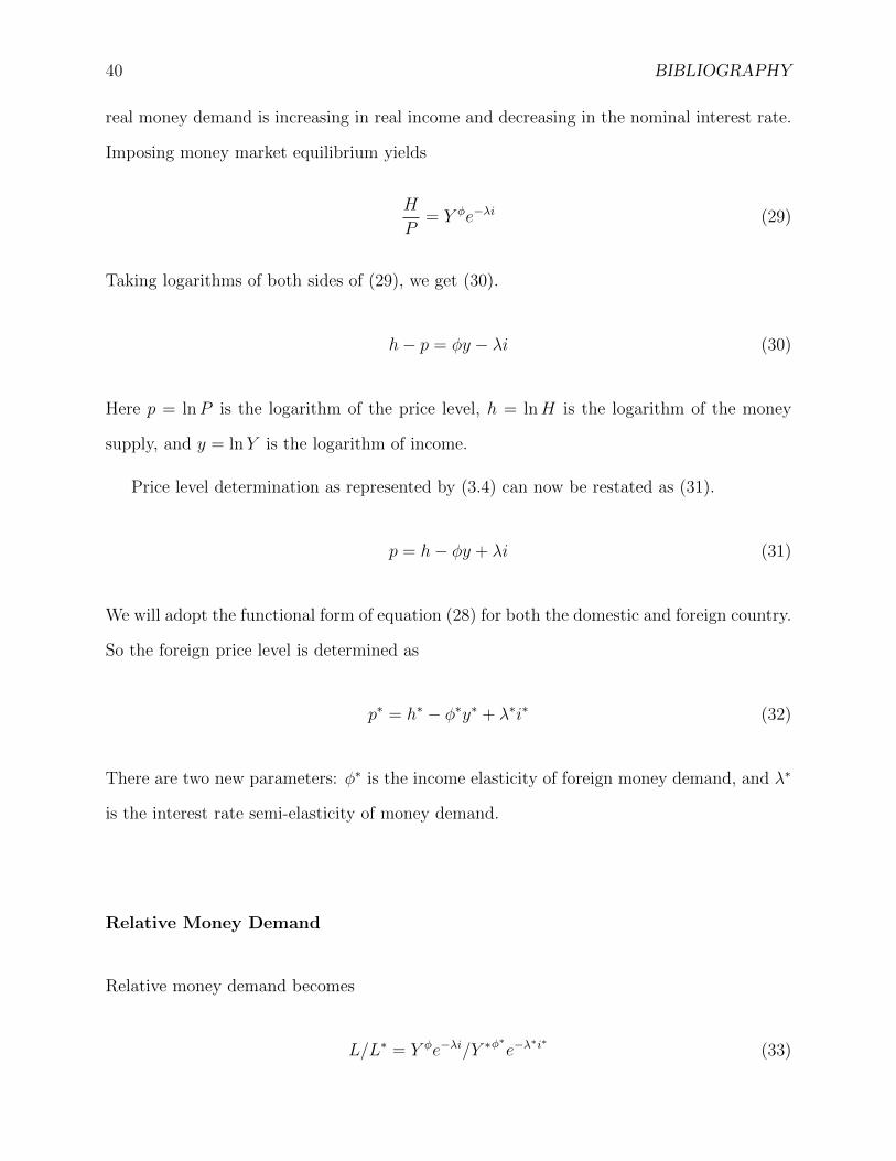
real money demand is increasing in real income and decreasing in the nominal interest rate.

Imposing money market equilibrium yields

H

P= Y φe−λi (29)

Taking logarithms of both sides of (29), we get (30).

h− p = φy − λi (30)

Here p = lnP is the logarithm of the price level, h = lnH is the logarithm of the money

supply, and y = lnY is the logarithm of income.

Price level determination as represented by (3.4) can now be restated as (31).

p = h− φy + λi (31)

We will adopt the functional form of equation (28) for both the domestic and foreign country.

So the foreign price level is determined as

p∗ = h∗ − φ∗y∗ + λ∗i∗ (32)

There are two new parameters: φ∗ is the income elasticity of foreign money demand, and λ∗

is the interest rate semi-elasticity of money demand.

Relative Money Demand

Relative money demand becomes

L/L∗ = Y φe−λi/Y ∗φ∗e−λ

∗i∗ (33)


With this specification of relative money demand, if we take the logarithm of (3.7), we get

the following restatement of the crude monetary approach.

st = q + ht − h∗t − (φyt − φ∗y∗t ) + (λit − λ∗i∗t ) (34)

Here p∗ = lnP ∗ is the logarithm of the foreign price level, h∗ = lnH∗ is the logarithm of the

foreign money supply, y∗ = lnY ∗ is the logarithm of foreign income, and i∗ is the foreign

interest rate.

.1.2 Testing the Monetary Approach

Of course we do not expect (34) to hold exactly. When we test the monetary approach, we

allow for temporary deviations from purchasing power parity and from our representation of

relative money demand to add an “error term” to (34). This lack of perfect fit forces us to

consider statistically based tests of the monetary approach, such as the early regression tests

of Hodrick (1978) and Putnam and Woodbury (1979–80) discussed in section 3.2.2. Using

monthly data from April 1973 to September 1975, Hodrick (1978, eq. 7) found the following

for the USD/DEM exchange rate.

s = 7.85 + 1.52h− 1.39h∗ + 2.53i+ 1.93i∗ − 2.23y + 0.073y∗ (35)

In section 3.2.2, we also noted that the monetary approach is usually developed under

the further assumption that the foreign and domestic countries have identical interest rate

semi-elasticities. In our log-linear specification, this implies that λ = λ∗, yielding (36).18

st = q + ht − h∗t − (φyt − φ∗y∗t ) + λ(it − i∗t ) (36)

18We also noted that some work assumes identical income elasticities (φ = φ∗) as well as identical interestrate semi-elasticities. Here is a quick way to develop the crude monetary approach under these assumptions.Note that by taking the logarithm of (3.2), purchasing power parity can be characterized by

st = q + pt − p∗t

42 BIBLIOGRAPHY

In this version of the crude monetary approach, the foreign and domestic interest rates enter

only as an interest rate differential (it−i∗t ), allowing us to substitute the the forward discount

from interest parity condition fd = i− i∗. This yields (37).

st = q + ht − h∗t − (φyt − φ∗y∗t ) + λfd t (37)

The numbers reported in table 5 are the estimated coefficients from equation 37, as we see

more explicitly in table 4.

Estimated Coefficient onStudy: Sample: fd h h∗ y y∗

Frenkel (1976) 1921.02–1923.08 0.591 0.975 – – –Bilson (1978b) 1972.01–1976.04 0.0228 1.0013 -1.0081 -1.0184 0.9990Bilson (1978a) 1970.04–1977.05 1.3853 1.0026 -0.9846 -0.9009 1.0183

Table 4: Germany/U.K.: Early Estimates of Equation (37)

Implicitly, Frenkel dumped domestic income and all foreign variables into the constant

term. His equation (4′′) is

s = −5.135 + 0.975h+ 0.591fd

As discussed in section 3.2.2, all the estimated coefficients are statistically significant, and

the coefficient on the money supply differs insignificantly from unity. This was viewed as

dramatic support for the monetary approach. The table reports equation (45) of Bilson

(1978b), which estimates a model of the DEM/GBP exchange rate using monthly data for

When domestic and foreign money demands have identical parameters, we have

ht − pt = φyt − λith∗t − p∗t = φy∗t − λi∗t

Solving these money market equilibrium conditions for prices and substituting into the PPP equation yields

st = q + ht − h∗t − φ(yt − y∗t ) + λ(it − i∗t )


the period 1972.01–1976.04. Despite considerable econometric manipulation to arrive at the

reported results, Bilson found the coefficient on fd not to be statistically different from zero.

Bilson (1978a) extends this sample to 1970.04–1977.05. The results reported in table 4 are

from his equation (12), which includes a time trend intended to capture trends in relative

money demand. His equation (12) is

s = −1.3280 + 1.0026h− 0.9846h∗ + 1.3853fd − 0.9009yt + 1.0183y∗t − 0.0049t

Although the estimated coefficient of -0.0049 on t appears small, a half a percent appreciation

of the DEM per month adds up. As discussed previously, all the coefficients are statistically

significant, and the coefficients on money supplies are close to unity.

44 BIBLIOGRAPHY

.2 Partial Adjustment of Money Demand

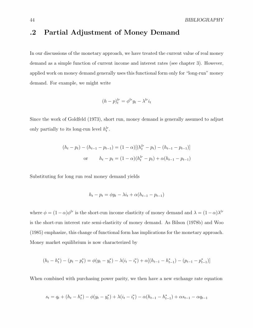
In our discussions of the monetary approach, we have treated the current value of real money

demand as a simple function of current income and interest rates (see chapter 3). However,

applied work on money demand generally uses this functional form only for “long-run” money

demand. For example, we might write

(h− p)lrt = φlryt − λlrit

Since the work of Goldfeld (1973), short run, money demand is generally assumed to adjust

only partially to its long-run level hlrt .

(ht − pt)− (ht−1 − pt−1) = (1− α)[(hlrt − pt)− (ht−1 − pt−1)]

or ht − pt = (1− α)(hlrt − pt) + α(ht−1 − pt−1)

Substituting for long run real money demand yields

ht − pt = φyt − λit + α(ht−1 − pt−1)

where φ = (1−α)φlr is the short-run income elasticity of money demand and λ = (1−α)λlr

is the short-run interest rate semi-elasticity of money demand. As Bilson (1978b) and Woo

(1985) emphasize, this change of functional form has implications for the monetary approach.

Money market equilibrium is now characterized by

(ht − h∗t )− (pt − p∗t ) = φ(yt − y∗t )− λ(it − i∗t ) + α[(ht−1 − h∗t−1)− (pt−1 − p∗t−1)]

When combined with purchasing power parity, we then have a new exchange rate equation

st = qt + (ht − h∗t )− φ(yt − y∗t ) + λ(it − i∗t )− α(ht−1 − h∗t−1) + αst−1 − αqt−1

.2. PARTIAL ADJUSTMENT OF MONEY DEMAND 45

Of course the inflation rate depends on many variables in the short run. In the monetary

approach model, however, attention centers on the rate of growth of the money supply, and

money supply growth rates (∆h and ∆h∗) are treated as exogenously set by the central

bank. The expected inflation differential is therefore treated as deriving from perceived

monetary policy. Recalling that for simplicity we are holding income constant, this implies

that when money growth rates are expected to be constant πe − π∗e = ∆he −∆h∗e. Under

such conditions, we can write our exchange rate determination equation as

S =H/H∗

L(∆he −∆h∗e, Y/Y ∗)(38)

However, when changes in monetary policy are anticipated, we cannot use (38).

We might try to avoid choosing an interest rate by turning to the Fisher equation, which

allows us to rewrite this as

st = λ(rt − r∗t ) + ht − h∗t − φ(yt − y∗t ) + λ(πet − π∗et )

If we treat the real interest rate differential as fixed, we no longer have to worry about

picking the right interest rate. But now we must worry about finding proxies for unobserved

expectations.

Capital Mobility

Suppose you are considering the purchase of an asset denominated in foreign currency. For

example, you might be a U.S. citizen contemplating the purchase of a Canadian bond. If

you expect the U.S. dollar to lose value (depreciate) against the Canadian dollar while you

hold the bond, this will raise your expected dollar returns from holding the Canadian bond.

Let us calculate the real returns, from the domestic perspective, to holding the domestic

46 BIBLIOGRAPHY

and foreign interest bearing asset. The real return from holding the domestic interest bearing

asset is i−π. The real return from holding the domestic interest bearing asset is i∗+∆s−π.

If the two assets are expected to have the same real return, then

i = i∗ + ∆se (39)

This is “uncovered interest parity” (UIP). When UIP holds, the interest differential equals

the expected rate of depreciation.

i− i∗ = ∆se (40)

The difference in the nominal rates of return is offset by an expected change in the price of

foreign exchange.

Uncovered interest parity is not implied by covered interest parity. Ensuring UIP requires

more than just frictionless financial markets. However, we can imagine special conditions

under which UIP should hold, so that the assets of two different currency denominations

should be expected to yield the same real returns. Suppose for example that investors are

indifferent as to the currency denomination of their assets as long as they have the same

expected return. That is, although investors care about their average returns they do not

care about the volatility of these return. In particular, they do not care about “currency

risk”. This situation is often referred to as perfect substitutability or risk neutrality, and it

implies that the expected real rate of return on the domestic asset equals the expected real

rate of return from holding the foreign asset: i−πe = i∗+ ∆se−πe. Perfect substitutability

implies uncovered interest parity (UIP):

i− i∗ = ∆se (41)

Note the UIP is an equilibrium condition, not a theory of interest rate determination.

It is a relationship that must hold when foreign and domestic assets are perfect substitutes.


This is a very strong condition on international capital markets. An even stronger condition

arises when we add a condition known as ex ante relative purchasing power parity, which

just says that changes in the real exchange rate cannot be anticipated. The idea that real

exchange rate changes cannot be anticipated is captured by treating the expected change in

the real exchange rate as zero: ∆qe = 0. From the definition of the real exchange rate, this

implies

∆se + π∗e − πe = 0 (42)

We will refer to this condition as expected PPP. It says that there is no expected change in

the real exchange rate. This may be because the real exchange rate has been constant and is

expected to stay that way. More realistically, expected PPP results when any past changes

in the real exchange rate are expected to be permanent.

Perfect substitutability and expected PPP together imply a very strong condition on

world capital markets. Combining expected (41) with (42), we see that the expected real

returns earned by domestic resident on domestic assets will equal the real returns expected

by foreign residents on foreign assets.

i− πe = i∗ − π∗e

This situation is known as real interest parity. Most empirical work on the monetary ap-

proach assumes expected PPP and UIP. However, some early tests of the monetary approach

took place under weaker assumptions than real interest parity, and we will begin by looking

at those.

48 BIBLIOGRAPHY

Real Interest Parity

Risk Neutrality

We now add a fourth standard component of the monetary approach to exchange rate de-

termination: the uncovered interest rate parity condition.

it − i∗t = ∆set

Substituting this into the crude monetary approach solution yields the standard flex-price

monetary approach solution for the behavior of the exchange rate:

st = ht − h∗t − φ(yt − y∗t ) + λ(∆set ) (43)

Immediately, we see that exchange rate expectations are a crucial determinate of the current

exchange rate. Unfortunately, these expectations are not directly observable. Empirical

tests of the monetary approach must therefore grapple with the problem of finding a useful

proxy for these expectations. We consider three approaches to modeling expectations in our

exchange rate models: the core inflation approach (Frenkel 1979), regressive expectations,

and rational expectations.

Expected PPP

Note that if purchasing power parity is expected to hold next period, then consistency

requires

set = pet − p∗et


This can be combined with the purchasing power parity condition for the current period to

yield a link between expected depreciation and the expected inflation differential.

∆set = πet − π∗et

We can therefore rewrite the standard monetary approach solution as the core inflation

approach.

st = ht − h∗t − φ(yt − y∗t ) + λ(πet − π∗et ) (44)

Comparing (44) with (43) makes it clear that this formulation just assumes away the contri-

bution of the real interest differential. Thus if we include a constant term in our empirical

work, say because we wish to allow for constant terms in the money demand equations, (44)

and (43) are not readily distinguishable.

Comment: some work has been done under the assumption of interest inelastic money

demand (e.g., Florentis et al. 1994). This yields the same models as above, with λ = 0.19

Comment: We have written

it − i∗t = ∆set

= πet − π∗et

Implying

it − πet = i∗t − π∗et

That is, open interest rate parity plus expected PPP implies real interest rate parity.

19The result is identical to that implied by the standard monetary approach when fundamentals follow arandom walk. (See the next chapter.)

50 BIBLIOGRAPHY

As discussed in the last chapter, this model is incomplete in that it does not include a

characterization of interest rate determination. We therefore introduced the Fisher equation

it = rt + πet

in order to characterize the interest rate differential as

it − i∗t = rt − r∗t + πet − π∗et (45)

Combining (.2) and (45) yields (46), the core-inflation characterization of the monetary

approach model.

st = q + ht − h∗t − φ(yt − y∗t ) + λ(rt − r∗t + πet − π∗et ) (46)

Equation (46) highlights some key insights of the monetary approach to flexible exchange

rates. Most important is the observation that, ceteris paribus, doubling the domestic money

supply doubles the exchange rate.20

So far we have simply reviewed the derivation of the core-inflation version of the monetary

approach model. We now observe that if PPP holds every period then informed individuals

should expect it to hold. That is, the expected depreciation of the exchange rate should

equal the expected-inflation differential.

∆se = πe − π∗e

This condition is known as expected purchasing power parity (EPPP). Under EPPP, the

20Note that among the ceteris held paribus is expected inflation. Note too that doubling the money supplyadds ln 2 to the log of the money supply.


monetary approach model of flexible exchange rates can be summarized as

s = h− h∗ − φ(y − y∗) + λ(se − s) (MAFE)

The key difference in this approach is that the real interest differential is constrained to zero.

But if we wish to determine absolute price levels in the two countries as well as their relative

price level, we need to explicitly add the Fisher effect and exogenous real interest rates. We

also need the assumption that (3.2) is expected to hold every period.

L(i, Y )

L∗(i∗, Y ∗)= L(i− i∗, Y/Y ∗)

This allows us to rewrite (3.7), the determination of the exchange rate, as (36).

S = QH/H∗

L(i− i∗, Y/Y ∗)(47)

The implied characterization of the foreign price level is given in (48), which is the foreign

country equivalent of (31).

p∗ = h∗ + φ∗y∗ − λ∗i∗ (48)

t

S

0

((((

tt0

h

0

((((

tt0

p,s

0 tt0

h−p

0

Figure 8: Increase H at t0

52 BIBLIOGRAPHY

lnX(t) − lnX(t − 1) = %∆X Application: Let us write real GDP as output per hour,

A, times the number of hours worked, H.

Y = AH (49)

This allows us to break real GDP growth into productivity growth and growth in hours

worked.

Y = A+ H (50)

For example, conventional wisdom places the potential growth rate of the U.S. economy

between 2.0 and 2.5 percent per annum. Labor force growth causes hours worked to rise

about 1% per year, and productivity growth makes up the other 1%–1.5% per year. In

the postwar period before 1973, productivity grew at an average of 3.2% per annum, which

yielded a much higher growth rate of GDP.

We can add some detail, when it is useful Hours worked can be written as the average

number of hours worked per worker, h, times the number of workers employed, N .

Y = AhN (51)

The number of workers employed is the labor force, L, times the employment rate, 1− u.

Y = Ah(1− u)L (52)

This allows us to break real GDP growth into productivity growth, labor force growth, and

reduction in unemployment.

Y = A+ h− u

1− uu+ L (53)

For example, conventional wisdom places the potential growth rate of the U.S. economy

between 2.0 and 2.5 percent per annum. The idea is that the labor force grows about 1%


per year, and productivity growth makes up the other 1%–1.5% per year. In the postwar

period before 1973, productivity grew at an average of 3.2% per annum, which yielded a

much higher growth rate of GDP.

Estimated Sensitivity of the Spot Rate to:Study: Sample: H H∗ Y Y ∗ fdFrenkel (1976) 1921.02–1923.08 0.975 – – – 0.591Bilson (1978b) 1972.01–1976.04 1.0013 -1.0081 -1.0184 0.9990 0.0228Bilson (1978a) 1970.04–1977.05 1.0026 -0.9846 -0.9009 1.0183 1.3853

Table 5: Germany/U.K.: Early Estimates of Equation (3.13)

lecture notes 3 the monetary approach to flexible exchange ... · the monetary approach to flexible...

Documents