monetary policy in the monetary approach to the …
TRANSCRIPT
MONETARY POLICY IN THE MONETARY APPROACH TO THE
BALANCE OF PAYMENTS: THE CASE OF ZAMBIA (1980-2011).
By
Yenda Goodwell Shamabobo
Computer #: 513803085
A Dissertation Submitted to the University of Zambia in Partial Fulfillment of the
Requirements of the Master of Arts Degree in Economics
THE UNIVERSITY OF ZAMBIA
2015

i | P a g e
DECLARATION
I (Yenda Goodwell Shamabobo) hereby declare that this dissertation:
1. Represents my bona fide work;
2. Has never been done by another researcher at this, or any other institution; and
3. Does not incorporate any other previous work without acknowledgement.
Signature: …………………………………………….
Date: ……………………………………………………..

ii | P a g e
COPYRIGHT
All rights reserved. No part of this dissertation must be produced and/ or stored in
any form without prior permission (in writing) from the author or the University of
Zambia.

iii | P a g e
CERTIFICATE OF APPROVAL
This dissertation of Yenda Goodwell Shamabobo has been approved as partial
fulfilment of the requirements for the award of Master of Arts Degree in
Economics by the University of Zambia;
Signature: …………………….. Date: ……………………………
Signature: …………………….. Date: ……………………………
Signature: …………………….. Date: ……………………………

iv | P a g e
ABSTRACT
The Zambian economy has been grappling with Balance of Payment (BoP)
problems since the mid-1970s. This led the country to resort to seeking support
from multilateral institutions and subsequently, the adoption of the IMF’s
structural adjustment programmes as a solution. The Monetary Approach to the
Balance of Payments (MABP) as an alternative to the Elasticities and Absorption
approaches, was generated by the Chicago School in the late 1960s and adopted by
the IMF in the 1970s as a means of solving BoP problems. Therefore, the IMF
prescribed policy solutions for BoP problems to Zambia and other countries were
largely based on the MABP. This study tried to establish the relevance and
significance of the MABP theory in the Zambian economy during the period 1980
to 2011. The research tested the MABP in Zambia by estimating the Reserve Flow
Equation (RFE) using OLS regression and joint hypotheses testing of the
preconditions outlined by the MABP using the F-Statistic. The research also
investigated the implications of monetary variables in the MABP in Zambia by
employing the SVAR model and estimating the underlying impulse reaction
functions (IRF). The hypothesis testing of both estimations, based on annual data
for the period 1980-2011 and monthly data for 1995 to 2011, led to the conclusion
that the MABP did not hold in Zambia for the study period. This implies that the
Zambian BoP is not purely a monetary phenomenon. It is worth noting that the
domestic price level (CPI) and domestic credit were found to be highly significant
in both the monthly and annual data regressions. The IRF analysis revealed that
changes in the domestic price level (CPI), domestic credit, and income (real GDP)
had significant impact on the BoP. A 1 percent shock in the CPI led to a positive
response from the BoP in the first 2 months then negative by the 5th
month, while a
1 percent shock in domestic credit resulted in a negative shock in the BoP in the
first 3 months, then positive by 5th
month and negative by the 7th
month. It was
also revealed that interest rates and the money multiplier did not have significant
impact on the BoP. Therefore, the research recommends that monetary authorities
in Zambia should consider using domestic credit as a tool for inducing stability in
the BoP, alongside other policies. This could be done through increased credit to
the private sector for production purposes at a lower cost as one of the strategies
for restoring (stabilising) positive performance of the BoP. The study also
recommends that the domestic price level could be used as an anchor not only in
managing domestic performance of the economy but also external performance.

v | P a g e
DEDICATION
To my father, Mr. Goodwell Shamabobo, who has given me unflinching support
throughout my education and my son, Kelvin Shibeu Bob Shamabobo, who was
born on the first day of classes of my Master’s Degree.
vi | P a g e
ACKNOWLEDGEMENTS
I would like to sincerely thank my Principle Supervisor, Dr. Chiselebwe
Ng’andwe, for the invaluable input and guidance rendered to me during this study.
My sincere gratitude also goes to my Econometrics mentor and Co-Supervisor, Dr.
Chrispin Mphuka, for the advanced analytical techniques he imparted in me
through the Master’s training and his immense contribution towards this study.
I would also like to thank my Supervisor at work, Mr. Kelvin Mpembamoto,
Assistant Director-Research and Planning Department at the Zambia Revenue
Authority for allowing me time to pursue my study amidst a busy work schedule.
In addition, I would like to thank the entire staff in the Research and Planning
Department at Zambia Revenue Authority for the support they rendered during the
time of my study.
My sincere gratitude also goes to members of staff of the Economics Department
at Bank of Zambia in particular, Mr. Joe Sichalwe, Statistical Assistant, Mr.
Chungu Kapembwa, Senior Researcher, and Mr. Peter Zgambo, Assistant
Director-Research, for the immeasurable support offered to me during data
collection. Let me also thank Mr. Litia Simbangala, Head-National Statistics at the
Central Statistics Office, for all the help rendered during the study.
The list would not be complete without thanking my parents for the moral support
during the Master’s programme. Special thanks to my wife, Mrs. Diana M.
Shamabobo, for the understanding and unquantifiable support rendered to me
during the entire duration of my study. Let me take this opportunity to also thank
my young brother, Hambweka Kelvin Shamabobo and cousin, Gideon Nsando as
well as the rest of the family for their moral support during the study.
I would like to convey my heartfelt gratitude to the Department of Economics at
the University of Zambia for hosting me as their student for the 2 year Master
Degree Programme. My acknowledgement would be incomplete if I did not thank
all the people that I have not mentioned as their part was critical to the success of
this study.
Above all, I would like to thank the Almighty Jehovah God for the guidance,
direction and good health that I have enjoyed throughout my entire academic life,
and for bringing close all those I have cited and those I have not cited (as the list is
endless) in this acknowledgement.
vii | P a g e
TABLE OF CONTENTS LIST OF FIGURES……………………………………………………..…..... ix
LIST OF TABLES……………………………………………………………. ix
ABBREVIATIONS AND ACRONYMS…………………………………….. x
CHAPTER 1 BACKGROUND AND INTRODUCTION ……..…………... 1
1.0 Overview………………………………………………………………. 1
1.1 About the Zambian Economy…………………………………………. 1
1.2 Statement of Problem………………….……………………………… 6
1.3 Study Objectives………………………………………………………. 7
1.3.1 General objective……………………..………..……………………. 7
1.3.2 Specific Objectives…………………………….……………………. 8
1.4 Hypotheses…………………………………………………………….. 8
1.5 Significance of Study……………………….…………………………. 8
1.6 Scope of the study……………………….….………………………….. 9
CHAPTER 2 EVOLUTION OF MACROECONOMIC POLICY IN
ZAMBIA……………………………………………………………………… 11
2.1 Overview………………………………………………………………. 11
2.2 Exchange Rate Policy……...……………………….………………….. 12
2.3 Monetary Policy………………………………….……………………. 14
CHAPTER 3 LITERATURE REVIEW………….…………………………. 17
3.0 Overview…………………..……………………………….………….. 17
3.1 The elasticity approach…………………..…………………………….. 17
3.2 The absorption approach………………………………………………. 18
3.3 The monetary approach………………………..………………………. 20
3.4 Empirical Evidence of MABP…………………...…………………….. 24
CHAPTER 4 METHODOLOGY……..…………………………………….. 28
4.1 Theoretical Framework…………………..……………………………. 28
4.2 The Reserve Flow model………...……………………………………. 29
4.2.1 The price level and the exchange rate in the model…………………. 33
4.3 The Structural Vector Autoregressive (SVAR) model……................... 34
4.4 Data Sources and Analysis……………………….…………………… 35
4.5 The Model Variables……………………………….…….…………… 36
CHAPTER 5 EMPIRICAL RESULTS…………………………..…………. 39
5.0 Overview…………………………………………………..…………… 39
5.1 Unit Root Tests…………………………………………..……………. 39
5.2 OLS Regression Results………………………………….…………… 41
5.3 Hypothesis Testing for the MABP…………………………………….. 45
5.4 SVAR and Impulse Response Functions………………………………. 48
5.6 Discussion………………………………………………..…………….. 53
CHAPTER 6 POLICY IMPLICATIONS AND CONCLUSION…………... 56
REFERENCES……………….………………………………………….……. 58

viii | P a g e
APPENDICES…………………..………………………………………..…… 65
Appendix 1: Unit Root Test Results……………..……….………………... 65
Appendix 2: OLS Regression Estimation Results…………………………. 66
Appendix 3: OLS Post Regression Diagnostic Tests………………………. 67
Appendix 4: VAR Outputs…………………………………………………. 67
Appendix 5: VAR Post Estimation Diagnostics……………….................... 70
Appendix 6: SVAR Outputs……………………………………………….. 74

ix | P a g e
LIST OF FIGURES
Figure 1: Real GDP Growth Rate in Zambia, 1966 to 2011……………………….... 2
Figure 2: Nominal Tax Revenue and Revenue Growth in Zambia, 1968 to 2011…. 3
Figure 3: Balance of Payments Developments in Zambia, 1970 to 2011…………… 5
Figure 4: Exchange Rate Development in Zambia, 1970 to 2011 (Nominal)……… 13
Figure 5: Movements in Monetary Variables, 1970 to 2011……………………….. 14
Figure 6: Developments in Money Supply, 1970 to 2011………………………….. 14
Figure 7: Response of International Reserves to a one percent shock in CPI………. 49
Figure 8: Response of International Reserves to a one percent shock in Domestic
Credit……………………………………………………………………………….. 50
Figure 9: Response of International Reserves to a one percent shock in Metal
Production (Real GDP)……………………………………………………………… 51
Figure 10: Response of International Reserves to a one percent shock in Multiplier.. 52
Figure 11: Response of International Reserves to a one percent shock in Wlbrate
(Interest Rates)……………………………………………………………………… 52
LIST OF TABLES
Table 1: Zambia's Per Capital Growth Rates in Comparison With Average of SSA.. 4
Table 2: Exchange Rate Regimes in Zambia, 1964 to 2011…………………..…… 12
Table 3: Unit Root Test Results, Monthly Data……………………………………. 40
Table 4: Unit Root Test Results, Annual Data………………………………………. 40
Table 5: Regression Estimates, Monthly Data………………………………………. 42
Table 6: Regression Estimates, Annual Data……………………...………………… 44
Table 7: Unit Root Test Results, Monthly Data………………….………………… 65
Table 8: Unit Root Test Results, Annual Data….……………….…………………. 65
Table 9: Regression Estimates, Monthly Data……………….…………………….. 66
Table 10: Regression Estimates, Annual Data…………………………………….. 66
Table 11: Summary of Post Regression Diagnostic Test Results………….………. 67

x | P a g e
ABBREVIATIONS AND ACRONYMS
BoP Balance of Payments
BoZ Bank of Zambia
CPI Consumer Price Index
CSO Central Statistics Office
DC Domestic Credit
FEMAC Foreign Exchange Management Committee
GDP Gross Domestic Product
IIP Index of Industrial Production
IMF International Monetary Fund
LDCs Least Developed Countries
MABP Monetary Approach to The Balance of Payments
NTEs Non-Traditional Exports
OGL Open General Licence
OLS Ordinary Least Squares
RCCs Reserve Currency Country
RFE Reserve Flow Equation
SAPs Structural Adjustment Programmes
SDR Special Drawing Rights
SSA Sub-Saharan Africa
SVAR Structural Vector Auto- Regression
WALBR Weighted Average Lending Base Rate
ZCCM Zambia Consolidated Copper Mines
ZRA Zambia Revenue Authority
1 | P a g e
CHAPTER 1
BACKGROUND AND INTRODUCTION
1.0 Overview
The International Monetary Fund (IMF) attaches a great deal of attention to the stability
of the balance of payments (BoP) for its member countries (Fleermuys 2005). Many
developing countries, Zambia inclusive, have been facing overall BoP problems. This is a
cause of concern because any country should aim at maintaining a stable equilibrium in
the balance of payments as one of the core objectives of macroeconomic policy. Several
factors account for the persistent balance of payments disequilibrium including: poor
export performance, huge service account deficits, external debt amortization, low inflow
of foreign direct investment, misappropriation of external funding support, excessive
domestic monetary and credit expansion, large fiscal deficits, price distortions and a
deterioration in the terms of trade (Ogiogio 1996; Obioma 1998).
1.1 About the Zambian Economy
The Zambian economy has gone through several cycles since independence which can be
categorized into six stages namely the pre-colonisation stage, colonization stage, post-
independence boom, economic decline of the 1970s and 1980s, economic reforms of the
1990s, and the most recent economic adjustments in the 2000s (World Bank, 2004).
Following independence Zambia adopted a Socialist economic model within an African
context. There was large-scale nationalisation of the mining industry and the creation of
large state owned conglomerates such as the Zambia Consolidated Copper Mines
(ZCCM). A considerable degree of central planning involving the setting up of a large
civil service followed as the government aimed to ensure self-sufficiency coupled with
industrial diversification. This period was relatively prosperous as the earnings from
mineral exploitation grew due to favourable copper prices. In the ten years following
2 | P a g e
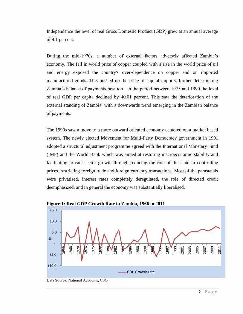
Independence the level of real Gross Domestic Product (GDP) grew at an annual average
of 4.1 percent.
During the mid-1970s, a number of external factors adversely affected Zambia’s
economy. The fall in world price of copper coupled with a rise in the world price of oil
and energy exposed the country's over-dependence on copper and on imported
manufactured goods. This pushed up the price of capital imports, further deteriorating
Zambia’s balance of payments position. In the period between 1975 and 1990 the level
of real GDP per capita declined by 40.01 percent. This saw the deterioration of the
external standing of Zambia, with a downwards trend emerging in the Zambian balance
of payments.
The 1990s saw a move to a more outward oriented economy centered on a market based
system. The newly elected Movement for Multi-Party Democracy government in 1991
adopted a structural adjustment programme agreed with the International Monetary Fund
(IMF) and the World Bank which was aimed at restoring macroeconomic stability and
facilitating private sector growth through reducing the role of the state in controlling
prices, restricting foreign trade and foreign currency transactions. Most of the parastatals
were privatised, interest rates completely deregulated, the role of directed credit
deemphasized, and in general the economy was substantially liberalised.
Figure 1: Real GDP Growth Rate in Zambia, 1966 to 2011
Data Source: National Accounts, CSO
(10.0)
(5.0)
-
5.0
10.0
15.0
19
66
19
68
19
70
19
73
19
75
19
77
19
80
19
82
19
84
19
86
19
88
19
90
19
93
19
95
19
97
19
99
20
01
20
03
20
05
20
07
20
09
20
11
%
GDP Growth rate
3 | P a g e
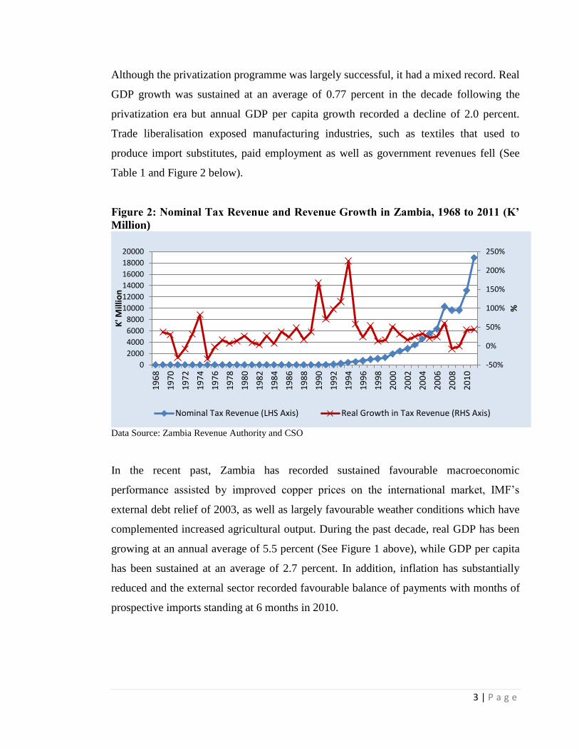
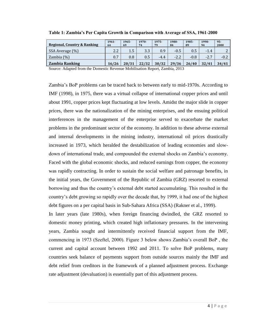
Although the privatization programme was largely successful, it had a mixed record. Real
GDP growth was sustained at an average of 0.77 percent in the decade following the
privatization era but annual GDP per capita growth recorded a decline of 2.0 percent.
Trade liberalisation exposed manufacturing industries, such as textiles that used to
produce import substitutes, paid employment as well as government revenues fell (See
Table 1 and Figure 2 below).
Figure 2: Nominal Tax Revenue and Revenue Growth in Zambia, 1968 to 2011 (K’
Million)
Data Source: Zambia Revenue Authority and CSO
In the recent past, Zambia has recorded sustained favourable macroeconomic
performance assisted by improved copper prices on the international market, IMF’s
external debt relief of 2003, as well as largely favourable weather conditions which have
complemented increased agricultural output. During the past decade, real GDP has been
growing at an annual average of 5.5 percent (See Figure 1 above), while GDP per capita
has been sustained at an average of 2.7 percent. In addition, inflation has substantially
reduced and the external sector recorded favourable balance of payments with months of
prospective imports standing at 6 months in 2010.
-50%
0%
50%
100%
150%
200%
250%
0
2000
4000
6000
8000
10000
12000
14000
16000
18000
20000
19
68
19
70
19
72
19
74
19
76
19
78
19
80
19
82
19
84
19
86
19
88
19
90
19
92
19
94
19
96
19
98
20
00
20
02
20
04
20
06
20
08
20
10
%
K' M
illio
n
Nominal Tax Revenue (LHS Axis) Real Growth in Tax Revenue (RHS Axis)
4 | P a g e
Table 1: Zambia’s Per Capita Growth in Comparison with Average of SSA, 1961-2000
Source: Adapted from the Domestic Revenue Mobilisation Report, Zambia, 2013
Zambia’s BoP problems can be traced back to between early to mid-1970s. According to
IMF (1998), in 1975, there was a virtual collapse of international copper prices and until
about 1991, copper prices kept fluctuating at low levels. Amidst the major slide in copper
prices, there was the nationalization of the mining enterprises, and the ensuing political
interferences in the management of the enterprise served to exacerbate the market
problems in the predominant sector of the economy. In addition to these adverse external
and internal developments in the mining industry, international oil prices drastically
increased in 1973, which heralded the destabilization of leading economies and slow-
down of international trade, and compounded the external shocks on Zambia’s economy.
Faced with the global economic shocks, and reduced earnings from copper, the economy
was rapidly contracting. In order to sustain the social welfare and patronage benefits, in
the initial years, the Government of the Republic of Zambia (GRZ) resorted to external
borrowing and thus the country’s external debt started accumulating. This resulted in the
country’s debt growing so rapidly over the decade that, by 1999, it had one of the highest
debt figures on a per capital basis in Sub-Sahara Africa (SSA) (Rakner et al., 1999).
In later years (late 1980s), when foreign financing dwindled, the GRZ resorted to
domestic money printing, which created high inflationary pressures. In the intervening
years, Zambia sought and intermittently received financial support from the IMF,
commencing in 1973 (Szeftel, 2000). Figure 3 below shows Zambia’s overall BoP , the
current and capital account between 1992 and 2011. To solve BoP problems, many
countries seek balance of payments support from outside sources mainly the IMF and
debt relief from creditors in the framework of a planned adjustment process. Exchange
rate adjustment (devaluation) is essentially part of this adjustment process.
Regional, Country & Ranking 1961-64
1965-69
1970-74
1975-79
1980-84
1985-89
1990-94
95-2000
SSA Average (%) 2.2 1.5 3.3 0.9 -0.5 0.5 -1.4 2
Zambia (%) 0.7 0.8 0.5 -4.4 -2.2 -0.8 -2.7 -0.2
Zambia Ranking 16/26 20/31 22/32 30/32 29/36 26/40 32/41 34/41

5 | P a g e
Figure 3: Balance of Payments Developments in Zambia, 1992 to 2011 (US$
Millions)
Data Source: Bank of Zambia
There are three key approaches followed in prescribing solutions for balance of payments
problems, namely, the Elasticities Approach, the Absorption Approach and the Monetary
Approach. This research concentrates on the latter approach but will also briefly discuss
the first two in the subsequent chapters. The origin of what has come to be known as the
Monetary Approach to the Balance of Payments (MABP) may be traced back to Hume's
specie flow mechanism which was rediscovered, revived and popularised in the 1960s as
an alternative approach to the BoP adjustment mechanisms. The approach is usually used
in financial programming as a sine qua non for the diagnosis of macroeconomic
problems, for example in the design and implementation of stabilization programmes
pursued under the auspices of the IMF (Khan, Montiel and Haque, 1986). Therefore, the
IMF support and prescribed solutions to the BoP problems that Zambia began facing in
the mid-1970s were somewhat based on the MABP.
The MABP basically explains the elimination of payments disequilibrium in terms of
factors bringing the demand and supply of money into equality. It treats the supply of
money as endogenous by assuming a feedback from the balance of payments through
-2500
-2000
-1500
-1000
-500
0
500
1000
1500
19
92
19
93
19
94
19
95
19
96
19
97
19
98
19
99
20
00
20
01
20
02
20
03
20
04
20
05
20
06
20
07
20
08
20
09
20
10
20
11
US$
Mill
ion
s
Overal BoP Current Account Capital Account

6 | P a g e
changes in international reserves to changes in the monetary liabilities of the central bank
and government (IMF, 1997). One of the important questions of monetary policy is the
extent to which the monetary authority (central bank) of an open economy can affect the
price level or the other arguments of the demand for money, such as the level of real
output and the interest rate. If it were the case that these could not be changed, then any
increase in monetary liabilities of the authority would be met by an equal and offsetting
outflow of international reserves (or an equi-proportionate rise in the price of home
goods and foreign exchange), and one would have to argue that monetary policy had no
influence on the real responses of the system.
Policy makers and scholars usually argue that the major cause of external imbalance that
Zambia has been experiencing for some time now is the adverse external development in
the international economy of the mid 1970s which saw the drastic drop in copper prices,
steep rise in oil prices and recession in western industrialised economies. It is also argued
that the socialist era between 1973 and 1985 in the country accounted for a significant
share of the BoP problems. It is however, noted that less empirical argument has been
forwarded on the extent to which valuation of the price level, the Kwacha exchange rate,
growth in domestic credit and other monetary variables in Zambia have explained the
external imbalance.
The aim of this study is therefore to establish the relevance of MABP in the Zambian
context during the period 1980 to 2011 and to study the significance of the roles of the
domestic price level, the money multiplier and credit policies in the determination of
balance of payments within the MABP by applying the Structural Vector Auto-
Regression (SVAR) method.
1.2 Statement of Problem
Zambia’s BoP problems emanated during the world economic recession of the mid-1970s
which saw the slump in copper prices and a sharp increase in oil prices on the
international market. In order to help curb these problems, Zambia resorted to seeking
7 | P a g e
policy and financial support from the IMF. Since the 1960s, the IMF BoP policies and
solutions have been monetary based (MABP) (IMF, 2004). Therefore, the BoP policy
solutions that there were prescribed to Zambia and other countries by the IMF were based
on the MABP. Hence, it was expected that after following these policies, Zambia’s BoP
would improve and stabilise and in the long-run reduce the occurrence of these problems.
However, for most of the period that the country was actively pursuing the MABP
policies, Zambia’s BoP was negative (See Figure 3 above). This discrepancy of the
validity of the MABP in solving Zambia’s BoP problems forms the motivation of this
research.
In literature, many arguments have been advanced as to why the country was still having
problems even after implementing the MABP policies; common among these are that the
long term effects of the 1970s world economic recession and those of the country’s
socialist era that existed between 1973 and 1985, still accounted for a significant share of
the Bop problems. Nevertheless, it is noted that less empirical studies have been carried
out to ascertain the extent to which the MABP has helped in alleviating Zambia’s BoP
problems, let alone to examine the extent to which movements of the price level, growth
in domestic credit, interest rates and other monetary variables in Zambia have explained
the external imbalance.
1.3 Study Objectives
1.3.1 General objective
The study aims at establishing the relevance of MABP in Zambia. This is done by
investigating the significance of the roles of the domestic price level and monetary policy
in the determination of balance of payments within the MABP in the Zambian context
and consequently,
8 | P a g e
1.3.2 Specific Objectives
1. To investigate the role of the domestic price level in the MABP in Zambia
2. To assess the impact of interest rates in the MABP in Zambia.
3. To establish the effect of domestic credit in the MABP in Zambia.
4. To establish the role of income in the MABP in Zambia.
1.4 Hypotheses
1. The domestic price level has no impact on the BoP in the MABP in Zambia.
2. Interest rates have no effect on the BoP in the MABP in Zambia.
3. Domestic credit has no impact on the BoP in the MABP in Zambia.
4. Income has no effect on the BoP in the MABP in Zambia.
1.5 Significance of Study
From around the 1970s, most least developed countries (LDCs), those in Africa
inclusive, implemented and continue to implement the IMF supported programmes such
as the Structural Adjustment Programmes (SAPS) and other financial system monitory
strategies (World Bank, 2004). Most of these programmes are based on MABP. Although
extensive studies to assess the relevance and significance of the MABP have been done
in other LDCs especially those in Latin America, little or no studies have been conducted
in the context of SSA.
A large research gap still exists in evaluating the approach against the African
experience. It should however be noted that, over the past decade, studies have emerged
in countries like Ghana, Nigeria, Malawi and Zimbabwe which have analysed the MABP
in the context of the respective economies. Similar empirical work on the subject known
to the researcher in the Zambian context is that of Peter Fairman (1986) who analysed the
applicability of the monetary approach in the balance of payments using 1970 to 1983

9 | P a g e
data and found that the approach holds up well in Zambia and that the monetary
processes despite the economic shocks in the said period were relatively stable.
This research is therefore significant as it tries to bridge the knowledge gap that exists in
evaluating the MABP significance in the Zambian and SSA context. Most importantly,
the study’s relevance and uniqueness is reinforced by the following; i) unlike other
studies in the Zambian and other African context, the study employs the SVAR model in
the determination of the roles of monetary policy variables in the MABP which will
make the findings empirically robust and theoretically consistent, ii) the study period
closely corresponds to the period when Zambia was actively receiving BoP support from
the IMF, and iii) the study offers a more recent examination of the MAPB in Zambia.
Given the BoP problems that Zambia has been experiencing, there is need to provide
more recent evidence to the monetary policy officials on the significance and
implications of the MABP in our economy. By examining the MABP, the research offers
a basis for understanding the relationship between monetary policy and BoP problems in
Zambia. The results will in this way provide renewed knowledge to policy makers on the
required mix of monetary policy instruments when trying to spur growth in the economy
while at the same time maintaining a healthy BoP (external balance), which is important
in the solving of BoP problems that the country may face in future. The study also adds
to the existing pool of knowledge for students of modern open macroeconomics and will
provide a basis for future research in the area in the Zambian context.
1.6 Scope of the study
The study will aim at evaluating the implications of the Zambian monetary policy within
the MABP over the period 1980 to 2011. The period has been chosen because it
coincides with the period when Zambia was actively receiving BoP support from the
IMF.

10 | P a g e
The rest of the research is outlined as follows; Chapter 2 reviews literature on the MABP
and alternative BoP approaches and Chapter 3 gives an account of the evolution of
macroeconomic policy in Zambia. Chapter 4 describes the methodology, followed by
Chapter 5 which gives the empirical findings of the study and also discusses the results.
Lastly but not the least, policy implications and conclusions are given in Chapter 6.

11 | P a g e
CHAPTER 2
EVOLUTION OF MACROECONOMIC POLICY IN ZAMBIA
2.0 Overview
Zambia’s macroeconomic policy has been largely shaped by the evolving political
system. Since independence, the country has seen three episodes, namely; the immediate
post-independence market-based policy under the Multi-Party political system (1964-
1973), the socialist policy under the One-Party State political system (1975-1990) and the
capitalist policy under the Multi-Party political system (1991 to date).
Due to the existing One-Party system with a socialist ideology, the period prior to 1991
was featured by a controlled economy. Consumer prices, interest rates, exchange rates
and credit allocation were administratively fixed by the State without any consideration
for market forces of demand and supply. In addition, the State owned all the companies
including mining firms which culminated into inefficiency in production and allocation
of national resources. In 1991 after the insurgence of a Multi-Party state, the economy
was liberalised and the macroeconomic policy was reformed to one characterised by
capitalist practices. During this period, markets and institutions were restructured with
Government influence being limited to policy direction. The economy reacted favourably
to the reforms resulting in restoration of stability in macroeconomic variables including
growth, tax revenues, money supply and inflation. Capital formation has increased
substantially (as a percentage of GDP) since 1992, and non-traditional exports and
services have been growing fast since the early 1990s and with copper production and
export increasing significantly (IMF, 2000). In addition, the international reserves
position has strengthened. The general business environment has also improved, with
increased volumes of foreign direct and portfolio investments driving resurgent private
sector led growth.
12 | P a g e
2.2 Exchange Rate Policy
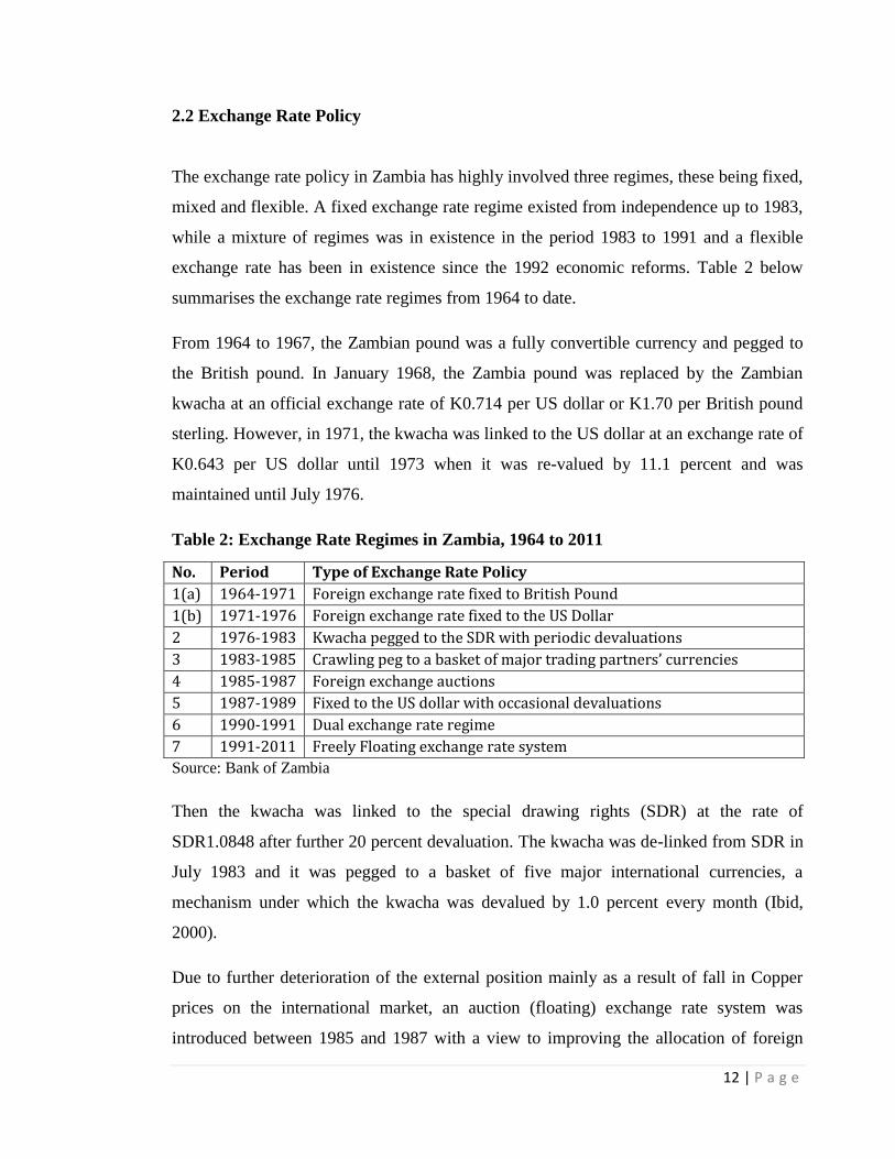
The exchange rate policy in Zambia has highly involved three regimes, these being fixed,
mixed and flexible. A fixed exchange rate regime existed from independence up to 1983,
while a mixture of regimes was in existence in the period 1983 to 1991 and a flexible
exchange rate has been in existence since the 1992 economic reforms. Table 2 below
summarises the exchange rate regimes from 1964 to date.
From 1964 to 1967, the Zambian pound was a fully convertible currency and pegged to
the British pound. In January 1968, the Zambia pound was replaced by the Zambian
kwacha at an official exchange rate of K0.714 per US dollar or K1.70 per British pound
sterling. However, in 1971, the kwacha was linked to the US dollar at an exchange rate of
K0.643 per US dollar until 1973 when it was re-valued by 11.1 percent and was
maintained until July 1976.
Table 2: Exchange Rate Regimes in Zambia, 1964 to 2011
Source: Bank of Zambia
Then the kwacha was linked to the special drawing rights (SDR) at the rate of
SDR1.0848 after further 20 percent devaluation. The kwacha was de-linked from SDR in
July 1983 and it was pegged to a basket of five major international currencies, a
mechanism under which the kwacha was devalued by 1.0 percent every month (Ibid,
2000).
Due to further deterioration of the external position mainly as a result of fall in Copper
prices on the international market, an auction (floating) exchange rate system was
introduced between 1985 and 1987 with a view to improving the allocation of foreign
No. Period Type of Exchange Rate Policy
1(a) 1964-1971 Foreign exchange rate fixed to British Pound
1(b) 1971-1976 Foreign exchange rate fixed to the US Dollar
2 1976-1983 Kwacha pegged to the SDR with periodic devaluations
3 1983-1985 Crawling peg to a basket of major trading partners’ currencies
4 1985-1987 Foreign exchange auctions
5 1987-1989 Fixed to the US dollar with occasional devaluations
6 1990-1991 Dual exchange rate regime
7 1991-2011 Freely Floating exchange rate system

13 | P a g e
exchange and eliminating the parallel underground exchange rate market that was
emerging at the time. Amidst significant depreciations and soaring inflation, the auction
system was abandoned in mid-1987 and replaced by a fixed exchange rate system with
careful devaluations administered by the Foreign Exchange Management Committee
(FEMAC). This system was in operation until 1990.
In 1990, a dual exchange rate system managed by FEMAC was adopted with a retail
window for importers, an Open General Licence (OGL) system, and an official window
with a lower rate. The OGL retail and official exchange rate were unified in 1991 with
the commencement of economic liberalisation. Foreign exchange bureaus were licenced
to operate in mid-1992 and allowed to determine their exchange rate freely. The supply
of foreign exchange to the export retention and bureau markets was increased
significantly by raising the non-traditional export retention entitlement to 100 percent and
by permitting others to sell foreign exchange to the bureaus (IMF, 1993). Figure 4 below
depicts the exchange rate movements from 1970 to 2011.
Figure 4: Exchange Rate Developments in Zambia, 1970 to 2011 (Nominal)
Data Source: Bank of Zambia
-
1,000.00
2,000.00
3,000.00
4,000.00
5,000.00
6,000.00
K/USD (Nominal)
14 | P a g e
After liberalisation, Zambia Consolidated Copper Mines (ZCCM) earnings were now
exchanged at the market rate as a way of integrating the foreign exchange market. The
official exchange rate was devalued by 30 percent and the rate of crawl accelerated to 8
percent per month. Further modifications of the OGL system were made in 1993 with
most exchange controls transferred to commercial banks and a dealing system was
established. To pave way for the full convertibility of the kwacha, the Exchanged Control
Act of 1965 was suspended in January 1994 resulting in the liberalisation of both the
current and capital accounts. To date the exchange rate system remains liberalised and
floating but under the sparing control by the Central Bank (Bank of Zambia, 2014).
2.3 Monetary Policy
In the period 1964 t0 1991, Zambia’s monetary policy was characterised by the
implementation of direct instruments for controlling monetary aggregates which saw
administratively fixing of interest rates, credit allocation control, and the use of core
liquid assets and statutory reserves requirements. In addition, the consumer prices were
fixed (Ibid, 2014). This resulted in deterioration of the economy evidenced by the
period’s high inflation, negative real interest rates, predominantly negative real GDP
growth, an unsustainable balance of payments position, increasing foreign debt and
shortage of essential commodities. In 1991, after heeding to the advice of the IMF and
World Bank, the economy was liberalised which brought in macroeconomic reforms
oriented towards the development of the private sector and the use of market-based
instruments to maintain price and financial systems’ stability (See Figure 5 and Figure 6).

15 | P a g e
Figure 5: Movements in Monetary Variables, 1970 to 2011
Data Source: Bank of Zambia and CSO
Figure 6: Developments in Money Supply, 1970 to 2011
Data Source: Bank of Zambia and CSO
0.0
500.0
1000.0
1500.0
2000.0
2500.0
0.0
20.0
40.0
60.0
80.0
100.0
120.0
140.0
160.0
180.0
200.0
19
70
19
72
19
74
19
76
19
78
19
80
19
82
19
84
19
86
19
88
19
90
19
92
19
94
19
96
19
98
20
00
20
02
20
04
20
06
20
08
20
10
Ind
ex
%
Inflation % BOZ Rate, % CPI (RHS Y-axis)
0
500
1000
1500
2000
2500
0
5000000
10000000
15000000
20000000
25000000
19
70
19
72
19
74
19
76
19
78
19
80
19
82
19
84
19
86
19
88
19
90
19
92
19
94
19
96
19
98
20
00
20
02
20
04
20
06
20
08
20
10
US$
Mill
ion
s
K' M
illio
ns
M2 (LHS Axis) Total Loans & Advances (LHS Axis)
International Reserves, $ (RHS Axis)
16 | P a g e
The liberalisation of the economy was initially accompanied by a sharp rise in inflation
due to the lack of a nominal anchor for monetary policy. Inflation, driven by a sharp
increase in broad money and domestic credit (predominantly to the government),
accelerated rapidly reaching a record high of 240 percent in July 1993. As the country
was implementing the policy prescriptions under the IMF and World Bank’s SAPs,
inflation rapidly declined to below 50 percent by mid-1994. Key policy adjustments
undertaken included (i) tightening of monetary policy that reduced broad money growth
from more than 200 percent in 1990 to around 70 percent in 1992 and sharply increased
nominal interest rates; and (ii) the introduction of a new fiscal policy rule designed to
commit the government to a balanced domestic budget, the “cash budget” that helped
reduce the deficit from around 10 percent in 1989 and 1990 to below 3 percent in 1992
(IMF, 2000).
17 | P a g e
CHAPTER 4
LITERATURE REVIEW
3.0 Overview
According to Fleermuys (2005), the balance of payments account records a country’s
international economic performance, with the two most significant accounts being the
current account and capital account. Whereas the current account records all transactions
of goods and services and unrequited transfers in a country, the capital account records
all exchanges and money capital for various kinds of real or financial assets. The latter
account is important as it relates domestic transactions to international transactions.
There are three key approaches to the balance of payments namely the elasticities
approach, the absorption approach and the monetary approach which is the main concern
of this research. Differences among these approaches have occasionally been the focus of
sharp controversy, most notably in the case of elasticity and absorption, and recently in
the case of the monetary approach as contrasted with the others.
3.1 The elasticity approach
The elasticity approach focuses on the current account of the balance of payments and is
concerned with the condition under which exchange rate changes can compensate for
price distortions in international trade, which are assumed to be the major cause of the
value of imports exceeding exports. The Marshallian partial equilibrium analysis is
applied to markets for exports and imports. Capital movements are assumed away and the
domestic price level varies with respect to the world price level. Whether an
improvement in the balance of payments occurs as a result of devaluation depends
crucially on the foreign elasticity of demand for exports and home elasticity of demand
for imports denoted ex and em, respectively. If the elasticity condition, that is, ex + em >
1 held, devaluation would improve the balance of payments (assuming of course that the
foreign exchange market was stable). This is called the Marshall-Lerner condition. If the
sum is equal to unity, a change in the exchange rate will leave the balance of trade

18 | P a g e
unchanged. If the sum is smaller than unity, depreciation will make the balance
unfavourable and an appreciation will make it more favourable (Harbeler, 1949).
There are considerable doubts about the efficacy of devaluation in developing countries.
It is argued that the elasticities of exports and imports are sufficiently low, therefore
devaluation cannot be expected to lead to an improvement of the balance of payments
(see, for instance, Miles, 1979; Kincaid, 1984; and Saidi, 1987). A similar source of
pessimism surrounds the lags in the response of the current account to relative price
changes. The argument is that trade volumes respond sluggishly to price changes because
of the inertia of importers switching domestic expenditure away from imports, and the
existence of contracts. Thus, in the short run, it is unlikely that domestic export earnings
following devaluation will increase by enough to offset the initial increase in the value of
expenditure on imports. This is the "J Curve effect" on the current account, where,
following devaluation, the balance of trade appears worse before it improves. Moreover,
the elasticity approach ignores any direct effects devaluation may have on the domestic
price level and domestic nominal wages.
3.2 The absorption approach
We have seen that in the elasticity approach to the analysis of devaluation, the effect of
exchange rate adjustments on BoP depends principally on the elasticities of imports for
home and foreign goods. This means that the relative price changes due to devaluation
will be a pointer to the substitution effects that will happen. In this analysis income is
assumed fixed. Thus, the income multiplier effects of devaluation are ignored. Alexander
(1952) criticizes the elasticity approach as a partial equilibrium analysis. Instead, he
proposes the absorption approach as an alternative. The central tenet of the absorption
approach is that a favourable configuration of price elasticities may not be sufficient to
produce a positive balance of payments effect resulting from devaluation, if devaluation
does not succeed in reducing domestic absorption. The starting point of the absorption
approach is the national income identity:

19 | P a g e
Y=C + I + G + X- M ………(1)
where Y = national income;
C = private consumption of goods and services purchased at home and
from abroad;
I = total investment, by firms as well as by government;
G = government expenditure on goods and services
X = exports of goods and services; and
M = imports of goods and services.
It should be noted that recently this national income identity has been used to explain the
current account as the difference between optimal savings and investment decisions
(Rosensweig, 1994). Combining C +1 + G expenditure terms into a single term, A,
representing domestic absorption (i.e., total domestic expenditure) and X - M terms into
B, net exports/trade balance, we get:
Y = A + B………. (2)
Equation 2 states that national income equals absorption plus the trade balance, or
alternatively
B = Y-A …….(2')
Equation 2' can be expressed in changes as shown below:
dB = dY - dA …….(2")
But changes in absorption depend on real income and other factors related to devaluation.
Taking these into account, changes in absorption dA can be expressed as:
dA = cdY – dD…….. (3)
where c = the propensity to absorb; and
d = the direct effect of devaluation on absorption.
Substituting Equation 3 into Equation 2 the result is:
20 | P a g e
dB = (l- c) dY + dD…… (4)
Machlup (1943) postulates that the principal effect of devaluation on income is
associated with the increased exports of the devaluing country and the induced
stimulation of domestic demand through the multiplier effect, provided the economy is
operating below full capacity. Alexander (1952) postulates two effects of the income
effect, namely the idle resources effect and the terms of trade effect. The idle resources
effect will result in an improvement in the balance of payments as long as the marginal
propensity to absorb, c, is less than unity. If c is equal to or greater than unity, the foreign
balance will not be improved as a result of improved output. Under such circumstances,
the devaluation will be effective in stimulating recovery, but not improving the foreign
balance except possibly through direct effects (Alexander, 1952). On the other hand, the
effect of income on the change in terms of trade is assumed to worsen the balance of
payments. Thus, when the devaluing country is at full employment, or c is equal to or
greater than unity, devaluation will improve the balance of payments through the direct
effect on absorption, that is, the expenditure reducing effect of devaluation. This
expenditure reducing effect occurs through three channels, namely, the real cash balance
(the most important effect), income redistribution and money illusion effects. The real
balance effect occurs when money holders accumulate cash due to the increase in the
general price level as a result of devaluation. This will result in a fall in real expenditure.
This increase in demand for cash holdings will also result in a rise in interest rates,
further reducing absorption through a reduction in investment. Thus, the real balance
effect has a direct and indirect effect. The redistribution of income effect occurs when
wages lag behind prices, such that prices increase at the expense of profit. If income is
shifted from individuals with high propensity to those with low propensity, absorption
will decline, and the balance of payments will improve.
3.3 The monetary approach
The monetary approach to the balance of payments is said to have been developed in the
1950s and 1960s by the IMF Research Department under Jacques J. P. Polak, and Harry

21 | P a g e
G. Jonson, Robert A. Mundell and their students at University of Chicago1. Empirical
work on the fundamental basis of the MABP has been conducted by scholars such as
Dornbusch (1971), Frenkel (1971), Johnson (1972), Laffer (1969), and Mundell (1968,
1971). Mundell (ibid.) emphasised that monetary factors, not real factors, exert the most
influence on the balance of payments through their effects on the currency and capital
accounts of a country. This approach contends that disequilibrium in a country’s balance
of payments shows an equivalent discrepancy between that economy’s money demand
and supply (Alawode, 1997).
In the monetary approach to the balance of payments, money market disequilibrium is
seen as a crucial factor that provokes balance of payments disequilibrium. The stock
imbalance between the demand for and supply of money causes external disequilibrium
or balance of payments disequilibrium. If people demand more money than is being
supplied by the central bank, then the excess demand for money would be satisfied by
inflows of money from abroad. On the other hand, if the central bank is supplying more
money than is demanded, the excess supply of money is eliminated by outflows of
money to other countries. In this approach, balance of payments imbalances will restore
equality between the demand for and supply of money in the absence of official
intervention. In other words, external disequilibrium is transitory and will self-equilibrate
in the long-run. The approach therefore looks beyond merchandise trade and incorporates
the important role of financial assets (Melvin, 1992).
The MABP, which regards the balance of payments as a “monetary phenomenon”,
expresses the relationship between a country’s balance of payments and its money supply
(Chacholiades, 1990). Furthermore, it argues that there is disequilibrium in the money
market if there are surpluses and deficits in the balance of payments. Deficits are caused
by money supply exceeding money demand, while surpluses are caused by money
demand exceeding money supply (Howard & Mamingi, 2002). The MABP, therefore,
largely emphasizes the monetary implications of balance of payments disequilibria. In
1 http://wps.aw.com/wps/media/objects/11358/11631194/Appendix_18.pdf

22 | P a g e
terms of prices, the MABP regards the general price level as the determinant of the real
value of nominal assets, money and international debt. Relative prices seem to play a
secondary role as they are considered to have only a transitory effect on the balance of
payments (Umer, et al., 2010).
The MABP specifies a money supply identity, money demand identity, and an
equilibrium condition. The model consists of the following equations:
Ms = (R+D) ··· ··· ··· (1)
Md = F(Y, P, I) ··· ··· ··· (2)
Ms = Md ··· ··· ··· (3)
Where; Ms = Money supply
R = International Reserves
D = Domestic credit
Md = Money demand
Y = Level of real domestic income
P = Price level
I = Rate of interest
The monetary theory holds that there is a positive relationship between money demand
and income (∂Md /∂Y>0), and between money demand and the price level (∂Md /∂P>0).
However, there is a negative relationship between money demand and the interest rate
(∂Md /∂I<0). If interest rates are increased, people will demand less money as the
opportunity cost of holding cash balances is increased, thus creating incentives for
investing in interest-bearing securities.
Then the reserve flow equation is written as :
ΔR = Δ [F(Y, P, I)] - ΔD ··· ··· ··· (4)
23 | P a g e
Equation (4) is the basic equation of the MABP, stating that the balance of payments is
the result of divergence between the growth of money demand and the growth of
domestic credit, whilst the monetary consequences of the balance of payments bring the
money market into equilibrium. With money demand being stable, an increase in
domestic credit will cause an equal and opposite change in international reserves. The
coefficient of ΔD is, therefore, known as an offset coefficient: it shows the extent to
which changes in domestic credit are offset by changes in international reserves. The
MABP envisages a value of minus unity for this coefficient in the reserve flow equation
(Dhliwayo, 1996). The MABP claims that balance of payments deficits result in
decreases in the money supply as a consequence of a loss in international reserves. This
loss in reserves will only be temporary, however, provided that monetary authorities do
not completely sterilise them. Many small economies experience persistent deficits in
their balance of payments because authorities use “credit policies and expenditure
policies to maintain levels of output and employment” (Howard & Mamingi, 2002).
The MABP regards money demand as a demand for a stock; therefore, the inflows or
outflows of money are regarded as the disequilibrium between desired and actual stocks,
which can be adjusted through an excess of income over expenditure or vice versa. The
differences between income and expenditure will be corrected when the flow of money
brings the desired and actual money stock back into equilibrium (Fleermuys 2005).
Monetary authorities only have an influence on the flow supply of money. They do not
have control over the stock of money supply. Therefore, it is assumed that, in the case of
countries with fixed exchange rates, money supply is endogenous. Monetary policy only
has an influence on the balance of payments through its control over credit creation. In
the modern, demand-determined world, where money supply is credit-driven and loans
make deposits, this argument has gained ground, especially as the banking systems of
countries develop (Fleermuys 2005). It is important for researchers to understand the
underlying propositions of the MABP. Kemp (1975) outlines the key characteristics of
the MABP as: the MABP maintains that the transactions recorded in the balance of
payments are essentially a reflection of monetary phenomena; only those BoP
24 | P a g e
transactions which have an influence on domestic and foreign monetary bases and thus
on domestic and foreign money supplies are considered in the MABP; the model assumes
efficient world market for goods, services, and securities; it is a theory of an automatic
adjustment; and it provides a framework within which one is able to assess the
differential impact of monetary disturbances which occur in a world in which there is at
least one Reserve Currency Country (RCC) as opposed to those occurring in a world with
no RCCs.
In terms of which of the three approaches to the BoP is better, MABP is often presented
as superior to the other two because of its unique feature that the money market is stable
and if there is any disequilibrium in the money market, an automatic adjustment process
is initiated, which restores equilibrium in the long-run. According to the MABP, any dis-
equilibrium in the money market is expected to be adjusted through changes in the
international reserve flows or in the exchange rate or both, depending on the existing
exchange rate regime (Chaudhary and Shabbir, 2004).
3.4 Empirical Evidence of MABP
A number of studies have been undertaken to test the MABP using data from both the
developed market economies and LDCs. Kreinin and Officer (1978) surveyed 37 studies
that tested the MABP in general and found that the number of studies they considered
yielded negative results and the number of studies that supported the MABP were
approximately equal, suggesting that the empirical evidence then was inconclusive. In the
same survey, 14 studies tested the reserve-flow model. Three (3) studies produced
negative, seven (7) mixed and four (4) positive results. Out of these 14 studies, five (5)
used data from LDCs and one study reported negative (Cheng and Sargen, 1975), three
mixed (Connolly and Taylor, 1975 and 1979; and Aghevli and Khan, 1977) and one
reported positive (Cox and Wilford, 1978) results. Further examination of these five
studies reveals that the Cheng and Sargen study, which produced negative results, and the
Cox and Wilford study, which produced positive results, used annual time series data
while those with mixed results used cross-section data. All of them applied ordinary least
25 | P a g e
squares (OLS) regression technique, except Aghevli and Khan (1977) who, in one of
their two specifications, used correlation analysis. Rivera-Batiz and Rivera-Batiz (1985)
have also concluded that even though a large number of empirical studies exists on the
monetary approach, covering a wide range of countries and time periods, the weight of
this evidence does not overwhelmingly support or reject the monetary approach. In
support of the proponents, Duasa (2007) employed the bound testing approach to
cointegration and error correction models developed within the Autoregressive
Distributed Lag (ARDL) framework and found a significant long-run relationship
between monetary variables and the Malaysian trade balance. Gulzar (2008) who
econometrically tested the significance of the MABP in Pakistan using data for the period
1990 to 2008, established that the MABP did not hold in Pakistan. He however, found
that the exchange rate and inflation had positive significant impacts on the BoP in
Pakistan.
As to the predictions of the MABP, some unanimity has been reported on the existence
of a demand for money function as hypothesised by the approach. Johnson (1977 ), for
example, points out, following Mundell (1968), that: 'The most robust specific
proposition is that, contrary to Keynesian predictions, the fastest-growing countries will
have the strongest (surplus) balance-of-payments positions because their demand for
money will tend to grow faster than the supply of domestic credit.' This observation is
supported by the studies reviewed by Kreinin and Officer (1978) who find that the
evidence on the effect of exogenous movements in income and the price level supports
the monetary approach. They, however, observe that the approach is less favourably
supported on the other predictions. Others, however, conclude that the signs of the
estimated coefficients confirm the postulated ones, that is, inflation and income growth
turn out to be positively associated with the balance of payments while domestic credit
creation, multiplier growth and interest rate increases are negatively related to the
balance of payments. Further, while the signs turn out as predicted, the magnitudes of the
coefficients are different from those predicted by the approach as specified in Equation
(5) (Rivera-Batiz and Rivera- Batiz, 1985).

26 | P a g e
In the African context, Silumbu D.E (1995) examined the roles of the exchange rate and
monetary policy in the MABP in Malawi through the reserve flow mechanism and found
that devaluation of the Malawian Kwacha led to loss of international reserves. He also
observed that domestic credit had a positive coefficient as expected from the MABP
model implying effective use of credit policy by the monetary officials. In Zimbabwe's
investigation of the MABP, it was revealed that money played a significant role in
determining the balance of payments during the period 1980 to 1991. It was also found
that there was a one-to-one negative relationship and strong link between domestic credit
and the flow of international reserves (Dhliwayo, 1996). Danjuma, F (2013) and Boateng
and Ayentimi (2013) econometrically analysed the applicability of MABP to Nigeria and
Ghana, respectively. The general conclusion in both papers was that the balance of
payments in both economies was a monetary phenomenon in line with similar studies in
other countries. In Zambia, Mutale (1983) in his MABP related study which focused on
money supply as influenced by domestic credit and international reserves using OLS on
Zambian data for the period 1970 to 1980, observed that international reserves did not
have a significant effect on the growth of money supply but domestic credit. He further
revealed that monetary policy was essentially determined by developments in the BoP
with a payment surplus leading to higher Government revenue collections and the
converse to a deficit.
Although the monetary approach has been commended for explaining the balance of
payments well, it has prompted criticism from other scholars as an approach that ignores
other parts of international trade in determining the balance of payments. The MABP has
been blamed for disregarding the fiscal and real factors that influence changes in the
balance of payments, whilst concentrating only on monetary factors (Umer, et al., 2010).
Contrary to these views, it can be stated that the monetary approach does not ignore these
factors. Valinezhad (1992) contends that “the MABP only asserts that the effect on the
balance of payments of a higher rate of economic growth should be analysed with the
tools of monetary theory”. Further, Bilquees (1989) who followed up the Aghevli and
Khan (1977) study of cross-section data on 39 LDCs including Pakistan, by applying the
same model to a single country Pakistan, found that the MABP failed to explain
international reserve movements in countries like Pakistan and India as monetary policy
27 | P a g e
as well as foreign exchange and capital markets were restrictive and highly controlled in
these economies. Bilquees (Ibid) went on to argue that in the majority of LDCs, financial
and commodity markets were very different from those in developed economies because
of features such as strict exchange controls which rendered currencies of these countries
almost inconvertible, in addition to which the capital markets are extremely limited and
governed by factors including political stability and approval of the developmental and
financial programmes of these countries by the IMF.
28 | P a g e
CHAPTER 4
METHODOLOGY
4.1 Theoretical Framework
The theoretical framework that was adopted in this thesis is the analysis of MABP model
based on the basic Reserve Flow Equation (RFE) as used by Silumbu (1995) in his paper
“Roles of exchange rate and monetary policy in the MABP in Malawi” and by Bilquees
(1989) in his study “MABP: The Evidence on Reserve Flow from Pakistan”. This model
is outlined in detail below. The key advantage of using the RFE is that it enables the
single-equation analysis of the MABP as opposed to using a macro-model. Thus, the
RFE is appropriate for this research as it is argued that for a small2 country such as
Zambia, the results from a single-equation analysis of the MABP and those from a
macro-model analysis are the same (Miller, 1986).
However, the econometric specification of the model that is employed is the Structural
Vector Auto-Regression (SVAR) model of the RFE in the MABP. The SVAR has been
chosen because of the method’s enrichment in the econometric analysis of fluctuations in
economic variables as result of policy changes. Two key strengths highlighted in all
studies that utilize SVAR models are that i) SVAR allows for the time varying variance
of monetary policy shocks via stochastic volatility specification and ii) it allows a
dynamic interaction between the level of endogenous variables in the VAR and line
varying volatility (Mumtaz and Zanetti, 2013). After the SVAR, an impulse-response
analysis of the model will be conducted.
Since the early 1980s, VAR models have become a standard tool for empirical analysis
by macroeconomists. They are easy to use, they are often more successful in predictions
than complex simultaneous models (Bahovec and Erjavec, 2009) and they are a priori
non-restrictive, that is, they do not require “incredible identification restrictions” (the
2 A small country is one which has no significant influence of the world prices, interest rate or incomes and
as such is a price taker on international markets (Miller, 1986).
29 | P a g e
often used phrase of Sims (Enders, 2003)). Models of structural vector auto-regressions
(SVAR) use the restrictions imposed by economic theory to identify the system, that is,
from a reduced form of shocks to obtain an economic interpretative function of the
impulse response.
Mumtaz and Zanetti (2013) employed a structural vector auto-regression (SVAR) model
to analyse the impact of the volatility of monetary policy. In their analysis they
established that the nominal interest rate, output growth, and inflation fall in reaction to
an increase in the volatility of monetary policy. Ravnik and Zilic (2010) in their paper on
the effects of fiscal policy in Croatia used the multivariate Blanchard-Perotti SVAR
methodology to analyze disaggregated short-term effects of fiscal policy on economic
activity, inflation and short-term interest rates where they found that the effects of
government expenditure shocks and the shock of government revenues are relatively the
highest on interest rates and the lowest on inflation.
4.2 The Reserve Flow model
The research employs the SVAR model of the basic reserve flow equation (RFE) variant
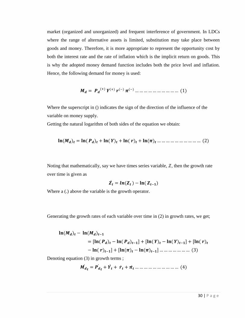
of the MABP. The basic MABP model assumes that there is a stable long-run demand for
money ( ) which positively depends on the domestic price level ( ) and real income
( ), negatively depends on the interest rate ) as the opportunity cost of holding cash
balances or as an inducement to wealth accumulation and is negatively related to the
domestic inflation rate3 ( ). As argued by Chaudhary and Shabbir (2004), the specific
features of underdeveloped economies, like Zambia, in terms of an impact of different
monetary variables are different from the case of developed countries. In less developed
economies, interest rate is included in money demand function as an opportunity cost
variable which remains one of the most controversial issues because in such economies,
interest rate is not determined by market forces due to the existence of dual money
3 It should be noted that although the interest rate embodies inflation, some scholars argue that in the case
of LDCs, where interest rates are generally fixed, the inflation rate is a better measure of opportunity cost
of holding cash balances (Haudhary and Habbir , 2004 and Bilqees, 1989). On this basis, the researcher
will in some cases interpret the two variables interchangeably.
30 | P a g e
market (organized and unorganized) and frequent interference of government. In LDCs
where the range of alternative assets is limited, substitution may take place between
goods and money. Therefore, it is more appropriate to represent the opportunity cost by
both the interest rate and the rate of inflation which is the implicit return on goods. This
is why the adopted money demand function includes both the price level and inflation.
Hence, the following demand for money is used:
Where the superscript in () indicates the sign of the direction of the influence of the
variable on money supply.
Getting the natural logarithm of both sides of the equation we obtain:
Noting that mathematically, say we have times series variable, , then the growth rate
over time is given as
Where a (.) above the variable is the growth operator.
Generating the growth rates of each variable over time in (2) in growth rates, we get;
Denoting equation (3) in growth terms ;

31 | P a g e
On the supply side of the money market, the supply of money ( ) is a multiple of the
high powered money (monetary base, ) and the money multiplier ( ). In turn, the high
powered money has two components: the domestic, which comprises domestic credit
( ), and the external, which comprises international reserves ( ). Thus:
Getting the natural logarithm of both sides of the equation, we get;
Using the growth rate principle outlined above to express (6) in growth terms we obtain;
(
)
Monetary equilibrium requires that supply of money equals demand for money, that is,
equating (4) to (7):
(
)
Expressing the balance of payments as a reserve-flow equation (that is, making term with
growth in international reserves as subject) under the assumptions of the MABP, relation
(8) becomes:
Under the assumptions of the MABP theory, the increase in the rate of growth of prices
( ) and real income ( ) will lead to an improvement in the balance of payments
(increase in stock of international reserves), while the increases in the growth rates of
inflation ( ), the interest rate ( ), the money multiplier ( ) and domestic credit ( )
will lead to loss of international reserves, holding all other factors constant (Bilquees,
1989).

32 | P a g e
Adding a constant, coefficients and the disturbance term to equation (9), the MABP is
empirical tested by the equation:
Where, , is a disturbance term.
According to the MABP, it is expected that:
i)
ii)
iii)
iv)
v) .
The joint MABP conditions (hypotheses) in i), ii) and iii) are joint tested using the F-
Statistic which is expresses as the ratio of a Wald statistic to the respective degrees of
freedom (Greene, 2012) defined as:
𝑭 𝒒 𝑿 𝑿 𝒒
𝒗˜𝑭 𝒗 𝒌
Where;
is a k*k variable matrix
𝑠 is k*k covariance matrix
is a v*k vector of restrictions
is a k*1 vector of parameters
𝑞 is the resultant v*1 vector from
is the number of restrictions
is the number of observations
33 | P a g e
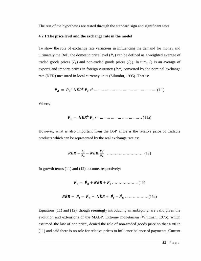
The rest of the hypotheses are tested through the standard sign and significant tests.
4.2.1 The price level and the exchange rate in the model
To show the role of exchange rate variations in influencing the demand for money and
ultimately the BoP, the domestic price level ( ) can be defined as a weighted average of
traded goods prices ( ) and non-traded goods prices ( ). In turn, is an average of
exports and imports prices in foreign currency ( *) converted by the nominal exchange
rate (NER) measured in local currency units (Silumbu, 1995). That is:
Where;
11a)
However, what is also important from the BoP angle is the relative price of tradable
products which can be represented by the real exchange rate as:
………………………..(12)
In growth terms (11) and (12) become, respectively:
……………….. (13)
………………(13a)
Equations (11) and (12), though seemingly introducing an ambiguity, are valid given the
evolution and extensions of the MABP. Extreme monetarism (Whitman, 1975), which
assumed 'the law of one price', denied the role of non-traded goods price so that a =0 in
(11) and said there is no role for relative prices to influence balance of payments. Current

34 | P a g e
monetarist thinking has incorporated the role of non-traded goods price in two respects.
From the money demand side, a rise in any component of the domestic price level
(due to devaluation and/or exogenous rise in ( *) raises the nominal demand for money,
other things being equal, relative to the domestic monetary base, and therefore leading to
an improvement in the BoP. This is the real balance effect.
The MABP model adopted in this study does not allow for distinguishing between
exports and imports or terms of trade movements as a separate relative price. However, to
gauge the empirical role of prices of tradable products and non-tradable product in
influencing BoP within the RFE of the MABP, the inflation components of (13) and
(13a) are substituted for the domestic price in (10). It should be recognized that a positive
coefficient for , as in (13), implies money demand effect while its negative coefficient,
as in (13a), means relative price effect on BoP.
4.3 The Structural Vector Autoregressive (SVAR) model
The general representation of a VAR(p) is
Where;
is a vector of k endogenous variables in the model.
is a k*k matrix of contemporaneous effects.
; and
is the error term satisfying;
i)
ii)
iii) ( )
From this VAR, the following Structural VAR may be obtained (Lutkepohl, 2005);
Where;

35 | P a g e
is a k*k matrix of contemporaneous effects
is a 1*k vector of shocks at time t, satisfying;
i)
ii)
iii) ( )
We can get the reduced form of the SVAR by pre-multiplying equation (15) by ;
Or
Where;
;
is the lag operator;
,
for all ; and
and is a vector of structural shocks that underlies the impulse reaction
functions.
Further, the research conducted times series unit root tests and other auxiliary statistical
tests as per econometric requirements. In addition, impulse response functions for the
variables at hand were generated.
4.4 Data Sources and Analysis
The study used secondary time series data for the period 1980 to 2011 obtained from the
Bank of Zambia (BoZ) and Central Statistical Office (CSO). The data obtained from the
Bank of Zambia included international reserves, nominal and real exchange rates,
market interest rates, Bank of Zambia interest rates, money supply, money demand,
commercial banks loans and advances, statutory reserves, currency in circulation, balance
36 | P a g e
of payments (BoP) and metal production. The data sourced from CSO included inflation,
real and nominal gross domestic product (GDP), consumer price index (CPI) and the
index of industrial production (IIP). The World Bank and IMF web based data sources,
and ZRA database were also consulted on a number of occasions. The data variables
were chosen in accordance to the requirements of the MABP model and other related
work done. Data analysis and management was conducted by use of statistical software
namely STATA and Excel.
4.5 The Model Variables
i) Domestic Credit
Under the assumptions of the MABP, increase in net domestic assets of the central bank
or domestic credit will lead to reduction in the stock of international reserves, holding all
other factors constant. Domestic credit is collated through the monetary survey conducted
by the Bank of Zambia on a monthly basis. The study could not access the full dataset on
domestic credit for period under consideration due to data unavailability and
unreliability. Therefore, the level of commercial bank loans and advances in kwacha
loans was used as a proxy for domestic credit.
ii) Gross Domestic Product (GDP)
The theory postulates that increases in the rate of growth of real income ( ) will lead to
an improvement in the balance of payments, ceteris paribus. For the estimations based on
monthly data, the study used the total production of Copper and Cobalt in Zambia as a
proxy for real GDP for the period under consideration. This is because real GDP and
mineral production (Copper and Cobalt) were seen to be moving together in the same
direction in the period under review and thus it was concluded that metal production
would be a good proxy for GDP. It is worth noting that Zambia’s GDP was largely
driven by mining activities during the period 1980 to 2005 (CSO, 2010). For the
37 | P a g e
estimations based on annual data, the actual real GDP series as recorded by CSO were
used.
iii) Interest rates
The MABP postulates that growth in the interest rate has a negative impact on
international reserves, holding all other factors constant. In Zambia, the Central Bank
Rate (BoZ rate) has traditionally formed the basis upon which commercial banks set their
interest rates. Commercial banks are the conduits of monetary policy. The desire of the
study was to use the Weighted Average Lending Base Rate (WALBR) for the
commercial banks as a proxy for the market interest rate. The monthly WLBR was
however not available for the period prior to 1994. Therefore, in the estimations based on
annual data, the study proxied the market interest rate using the BoZ rate.
iv) The Money Multiplier
Under the MABP, it is assumed that the increase in the rate of the money multiplier will
lead to less international reserves, holding all other factors constant. The money
multiplier is expressed as the ratio of reserve money in the domestic currency to money
supply (IMF, 2014). The researcher was able to access reliable and complete (both
monthly and annual) data on money supply in Zambia, at the M2 level. According to
Mishkin (2004), M2 can be defined as the total summation of currency in circulation,
traveller’s checks, demand deposits, other checkable deposits, small-denomination time
deposits and repurchase agreements, savings deposits and money market deposit
accounts, and money market mutual fund shares (non-institutional) in the economy.
Therefore, the study assumed money supply at M2 level. In this regard, the multiplier
was computed by dividing the M2 into Kwacha reserves held by commercial banks at
BoZ.
v) Price level and inflation
Data on both Consumer Price Index (CPI or price level) and inflation was available on
both monthly and annual basis for the entire study period. The MABP assumes that

38 | P a g e
increase in the growth of the price level (inflation) will lead to increase in the growth of
international reserves, holding all other factors constant, while increase in the rate of
growth of inflation (depreciation) leads to deterioration in the stock of international
reserves, ceteris paribus.
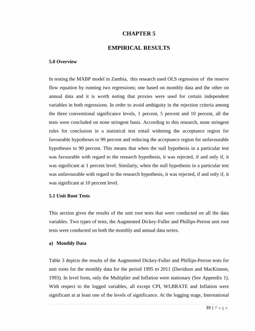
39 | P a g e
CHAPTER 5
EMPIRICAL RESULTS
5.0 Overview
In testing the MABP model in Zambia, this research used OLS regression of the reserve
flow equation by running two regressions; one based on monthly data and the other on
annual data and it is worth noting that proxies were used for certain independent
variables in both regressions. In order to avoid ambiguity in the rejection criteria among
the three conventional significance levels, 1 percent, 5 percent and 10 percent, all the
tests were concluded on none stringent basis. According to this research, none stringent
rules for conclusion in a statistical test entail widening the acceptance region for
favourable hypotheses to 99 percent and reducing the acceptance region for unfavourable
hypotheses to 90 percent. This means that when the null hypothesis in a particular test
was favourable with regard to the research hypothesis, it was rejected, if and only if, it
was significant at 1 percent level. Similarly, when the null hypothesis in a particular test
was unfavourable with regard to the research hypothesis, it was rejected, if and only if, it
was significant at 10 percent level.
5.1 Unit Root Tests
This section gives the results of the unit root tests that were conducted on all the data
variables. Two types of tests, the Augmented Dickey-Fuller and Phillips-Perron unit root
tests were conducted on both the monthly and annual data series.
a) Monthly Data
Table 3 depicts the results of the Augmented Dickey-Fuller and Phillips-Perron tests for
unit roots for the monthly data for the period 1995 to 2011 (Davidson and MacKinnon,
1993). In level form, only the Multiplier and Inflation were stationary (See Appendix 1).
With respect to the logged variables, all except CPI, WLBRATE and Inflation were
significant at at least one of the levels of significance. At the logging stage, International
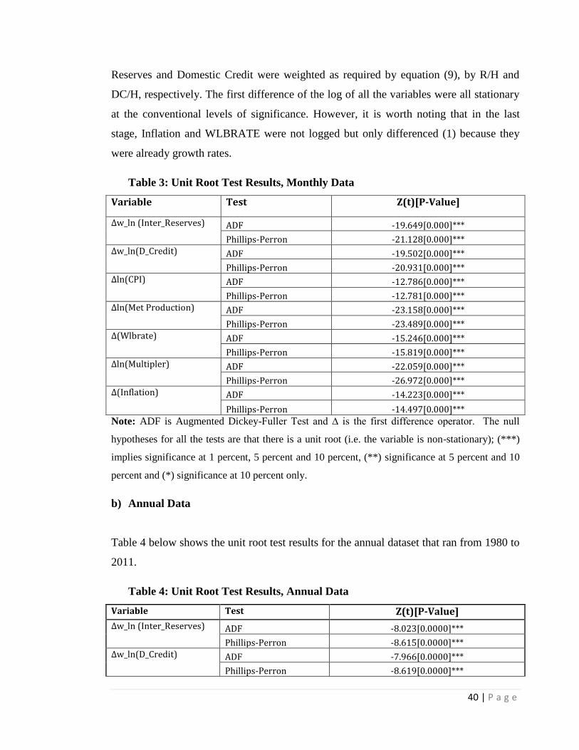
40 | P a g e
Reserves and Domestic Credit were weighted as required by equation (9), by R/H and
DC/H, respectively. The first difference of the log of all the variables were all stationary
at the conventional levels of significance. However, it is worth noting that in the last
stage, Inflation and WLBRATE were not logged but only differenced (1) because they
were already growth rates.
Table 3: Unit Root Test Results, Monthly Data
Variable Test Z(t)[P-Value]
∆w_ln (Inter_Reserves) ADF -19.649[0.000]***
Phillips-Perron -21.128[0.000]*** ∆w_ln(D_Credit) ADF -19.502[0.000]***
Phillips-Perron -20.931[0.000]*** ∆ln(CPI) ADF -12.786[0.000]***
Phillips-Perron -12.781[0.000]*** ∆ln(Met Production) ADF -23.158[0.000]***
Phillips-Perron -23.489[0.000]*** ∆(Wlbrate) ADF -15.246[0.000]***
Phillips-Perron -15.819[0.000]*** ∆ln(Multipler) ADF -22.059[0.000]***
Phillips-Perron -26.972[0.000]*** ∆(Inflation) ADF -14.223[0.000]***
Phillips-Perron -14.497[0.000]***
Note: ADF is Augmented Dickey-Fuller Test and ∆ is the first difference operator. The null
hypotheses for all the tests are that there is a unit root (i.e. the variable is non-stationary); (***)
implies significance at 1 percent, 5 percent and 10 percent, (**) significance at 5 percent and 10
percent and (*) significance at 10 percent only.
b) Annual Data
Table 4 below shows the unit root test results for the annual dataset that ran from 1980 to
2011.
Table 4: Unit Root Test Results, Annual Data
Variable Test Z(t)[P-Value]
∆w_ln (Inter_Reserves) ADF -8.023[0.0000]***
Phillips-Perron -8.615[0.0000]*** ∆w_ln(D_Credit) ADF -7.966[0.0000]***
Phillips-Perron -8.619[0.0000]***

41 | P a g e
∆(CPI) ADF 11.115[0.000]***
Phillips-Perron 7.092[0.000]*** ∆ln(GDP) ADF -5.397[0.0000]***
Phillips-Perron -5.438[0.0000]*** ∆(BoZrate) ADF -6.545[0.0000]***
Phillips-Perron -6.572[0.0000]*** ∆ln(Multiplier) ADF -6.949[0.000]***
Phillips-Perron -7.708[0.000]*** ∆(Inflation) ADF -5.211[0.0000]***
Phillips-Perron -5.231[0.0000]***
Note: ADF is Augmented Dickey-Fuller Test and ∆ is the first difference operator. The null
hypotheses for all the tests are that there is a unit root (i.e. the variable is non-stationary); (***)
implies significance at 1 percent, 5 percent and 10 percent, (**) significance at 5 percent and 10
percent and (*) significance at 10 percent only.
In level form, all variables with exception of Inflation and BoZ rate were stationary at the
three (3) levels of significance. The log of the values of the weighted Domestic Credit
and the Multiplier were stationary at all levels of significance under both tests, whereas
real GDP was found to be stationary under the Phillips-Perron test. The first differences
of log of all variables except for CPI were stationary at the three (3) levels of significance
(See Appendix 1). Therefore, in regression based on annual data, CPI was taken in its
level form while the logged values of the rest of the variable were used.
5.2 OLS Regression Results
The MABP model was estimated by running equation 10 (the RFE) using both monthly
and annual data with the purpose of adequately evaluating whether the MABP theory was
holding in Zambia. In the monthly regression, metal production (met production was
used as proxy for real GDP due to the non-measurement of GDP on either a quarterly or
monthly basis during the period under consideration. In the annual regression, the Bank
of Zambia rate (bozrate was used as a proxy for interest rates due to the unavailability
of the long series for the study period.

42 | P a g e
a) Monthly
The results of the regression based on monthly data with the dependent variable being the
growth rate in weighted international reserves, ∆w_ln(ireserves , are presented in the
table below. It is worth noting that for the rest of the paper, international reserves and
BoP are taken to mean one and the same thing, so the two terms are used
interchangeably.
Table 5: Regression Estimates, Monthly Data
Dependent Variable: :∆w_ln(ireserves Independent Variable Coefficient
(Standard Error) 1. ∆ln(cpi 1.323241***
(.1056806) 2. ∆ln(met production 0.0493561
(0.0312613) 3. ∆(wlbrate 0.0022921
(0.002262) 4. ∆(inflation 0.0020388
(.0018203) 5. ∆ln(multiplier 0.0662149**
(0. 0276548) 6. ∆w_ln(dcredit -1.032645***
(0. 0031031) 7. constant 0.0024493
(0. 0064445) Adjusted R-Squared=0.9983 Note: Figure in brackets is standard error, *** implies significance at 1 percent, 5 percent and 10
percent, ** significance at 5 percent and 10 percent and * significance at 10 percent only.
The estimation results reveal that the coefficient for CPI is highly significant at all
conventional levels of significance. The CPI coefficient of approximately 1.32 implies
that for a 1 percent increase in the rate of growth of the CPI (inflation), the rate of change
in the International Reserves increases by 1.32 percent. We can therefore conclude that
the rate of change in the domestic price level in Zambia has a significant positive impact
on the rate of change of International Reserves.

43 | P a g e
Metal Production which was a proxy for GDP in the regression was found to be
insignificant at all conventional levels. Nonetheless, the sign of the coefficient of 0.049
on metal production was positive thus in accordance with the expectations of the MABP.
Similarly, the third variable in the regression, WLBRATE (weighted average lending
base rate) was also found to be insignificant at all levels of significance but of the correct
sign as postulated by the MABP.
The rate of growth of Inflation (depreciation rate of local currency) was also found to be
insignificant at all levels of significance in the monthly data regression. In addition, the
sign of the coefficient for Inflation was also not consistent with expectation of the
MABP.
The coefficient on the Multiplier was significant at 5 percent level of significance. The
coefficient of approximately 0.066 meant that for every 1 percent increase in the rate of
growth of the money multiplier, there is a 0.066 percent increase in the rate of growth of
International Reserves .Put differently, for every 100 percent increase in the rate of
growth of the multiplier, there is a 6.6 percent increase in the rate of growth of
International Reserves. This therefore implies that growth in the Multiplier has a positive
influence in the rate of growth of International Reserves in Zambia.
More importantly, the coefficient on Domestic Credit (total loans and advances in the
economy) was found to be highly significant as evidenced by its P-Value of
0.000***.The coefficient of -1.033 on Domestic Credit implies that for every 1 percent
increase in the rate of growth of the Domestic Credit, there is a 1.033 percent reduction in
the rate of growth of International Reserves. It is worth noting that the negative sign of
the coefficient is in agreement with the expectation of the MABP. The finding implies
that changes in Domestic Credit (commercial banks loans and advances) have a negative
impact on the changes in Zambia’s International Reserves.
The constant was found to be insignificant at all conventional levels of significance. This
implies that if all other factors were fixed (zero), the increase in the growth of
International Reserves would be zero.

44 | P a g e
The adjusted R-Squared of approximately 99.8 percent means that the independent
variables in the model together or that the model, accounts for about 99.8 percent of the
variations that take place in International Reserves.
b) Annual
The results of the regression based on monthly with the dependent variable being the
growth rate in weighted international reserves, ∆w_ln(ireserves , are presented in the
table below.
Table 6: Regression Estimates, Annual Data
Dependent Variable: :∆w_ln(ireserves Independent Variable Coefficient 1. ∆(cpi 0.5455456***
(0.1824094) 2. ∆ln(cgdp -0.3361475
(1.208522) 3. ∆(bozrate 0.0019394
(0.0045635) 4. ∆(inflation -0.0003117
(0. 0019005) 5. ∆ln(multiplier 0.0196897
(0. 0862556) 6. ∆w_ln(dcredit -1.026496***
(0 .0106947) 7. constant 0.1704661**
(.0807734) Adjusted R-Squared =99.70%
The CPI was revealed to be significant at all conventional levels of significance. The
coefficient of approximately 0.546 on CPI implies that for every 1 percent increase in the
growth rate of CPI there is a 0.546 percent increase in the growth rate of International
Reserves. This finding is in tandem with the finding in the estimation that used monthly
data.
The real GDP, BoZ rate, Inflation and the Multiplier were all found to be insignificant in
the estimation using annual data. This implies that each of these variables did not have
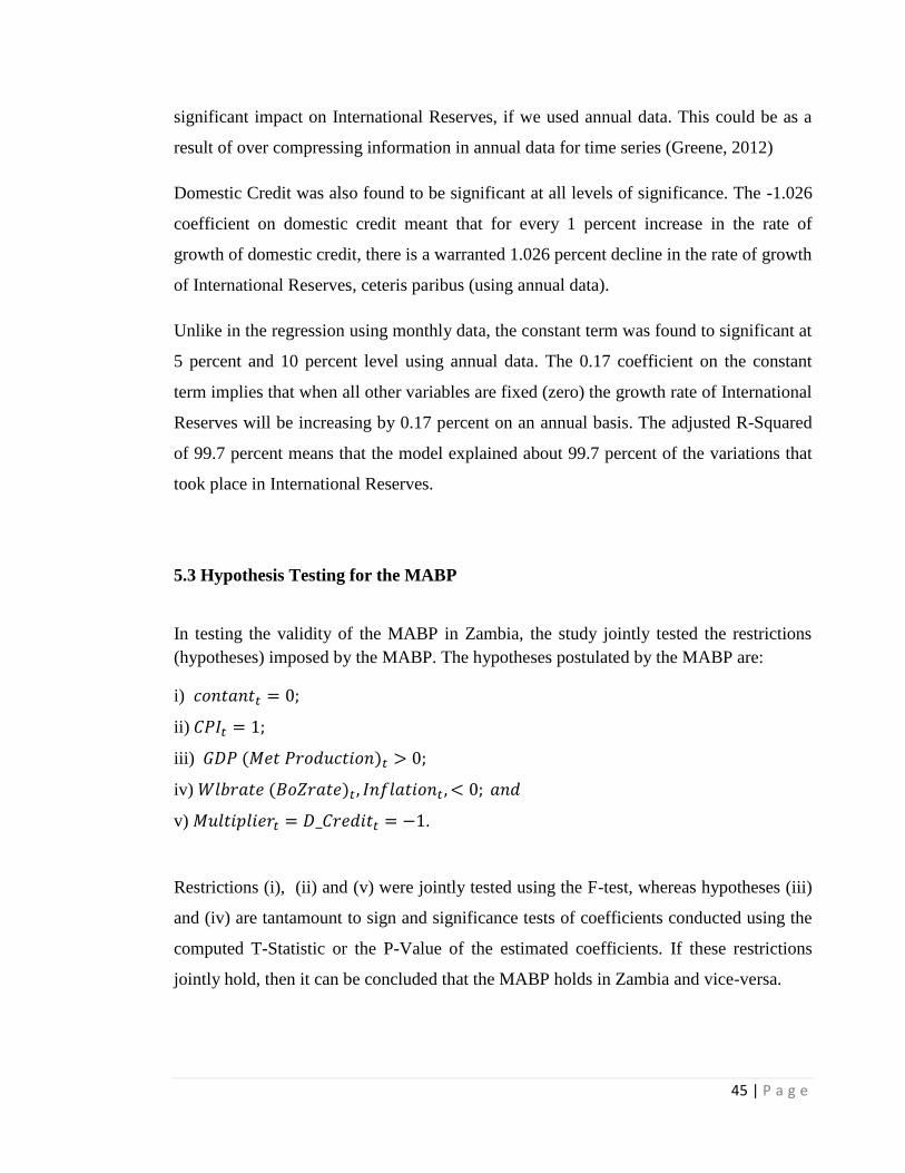
45 | P a g e
significant impact on International Reserves, if we used annual data. This could be as a
result of over compressing information in annual data for time series (Greene, 2012)
Domestic Credit was also found to be significant at all levels of significance. The -1.026
coefficient on domestic credit meant that for every 1 percent increase in the rate of
growth of domestic credit, there is a warranted 1.026 percent decline in the rate of growth
of International Reserves, ceteris paribus (using annual data).
Unlike in the regression using monthly data, the constant term was found to significant at
5 percent and 10 percent level using annual data. The 0.17 coefficient on the constant
term implies that when all other variables are fixed (zero) the growth rate of International
Reserves will be increasing by 0.17 percent on an annual basis. The adjusted R-Squared
of 99.7 percent means that the model explained about 99.7 percent of the variations that
took place in International Reserves.
5.3 Hypothesis Testing for the MABP
In testing the validity of the MABP in Zambia, the study jointly tested the restrictions
(hypotheses) imposed by the MABP. The hypotheses postulated by the MABP are:
i)
ii)
iii)
iv)
v) .
Restrictions (i), (ii) and (v) were jointly tested using the F-test, whereas hypotheses (iii)
and (iv) are tantamount to sign and significance tests of coefficients conducted using the
computed T-Statistic or the P-Value of the estimated coefficients. If these restrictions
jointly hold, then it can be concluded that the MABP holds in Zambia and vice-versa.
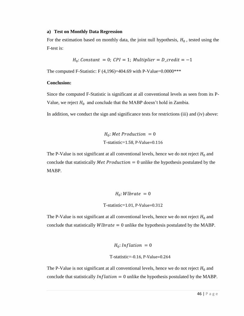
46 | P a g e
a) Test on Monthly Data Regression
For the estimation based on monthly data, the joint null hypothesis, tested using the
F-test is:
𝑠
The computed F-Statistic: F (4,196)=404.69 with P-Value=0.0000***
Conclusion:
Since the computed F-Statistic is significant at all conventional levels as seen from its P-
Value, we reject and conclude that the MABP doesn’t hold in Zambia.
In addition, we conduct the sign and significance tests for restrictions (iii) and (iv) above:
T-statistic=1.58, P-Value=0.116
The P-Value is not significant at all conventional levels, hence we do not reject and
conclude that statistically unlike the hypothesis postulated by the
MABP.
T-statistic=1.01, P-Value=0.312
The P-Value is not significant at all conventional levels, hence we do not reject and
conclude that statistically unlike the hypothesis postulated by the MABP.
T-statistic=-0.16, P-Value=0.264
The P-Value is not significant at all conventional levels, hence we do not reject and
conclude that statistically unlike the hypothesis postulated by the MABP.

47 | P a g e
On the basis of the test results revealed above, it can be concluded that the MABP does
not hold when tested using Zambian monthly data.
b) Test on Annual Data Regression
For the estimation based on annual data, the joint null hypothesis, tested using the F-
test is:
𝑠
The computed F-Statistic: F (4,24)=49,000,000 with P-Value=0.0000***
Conclusion:
Since the computed F-Statistic is significant at all levels as seen from its P-Value, we
reject and conclude that the MABP does not hold in Zambia.
Similarly, we conduct the sign and significance tests for restrictions (iii) and (iv):
T-statistic=-0.28, P-Value=0.783
The P-Value is not significant at all conventional levels, hence we do not reject and
conclude that statistically unlike the hypothesis postulated by the MABP.
T-statistic=0.42, P-Value=0.675
The P-Value is not significant at all conventional levels, hence we do not reject and
conclude that statistically unlike the hypothesis postulated by the MABP.
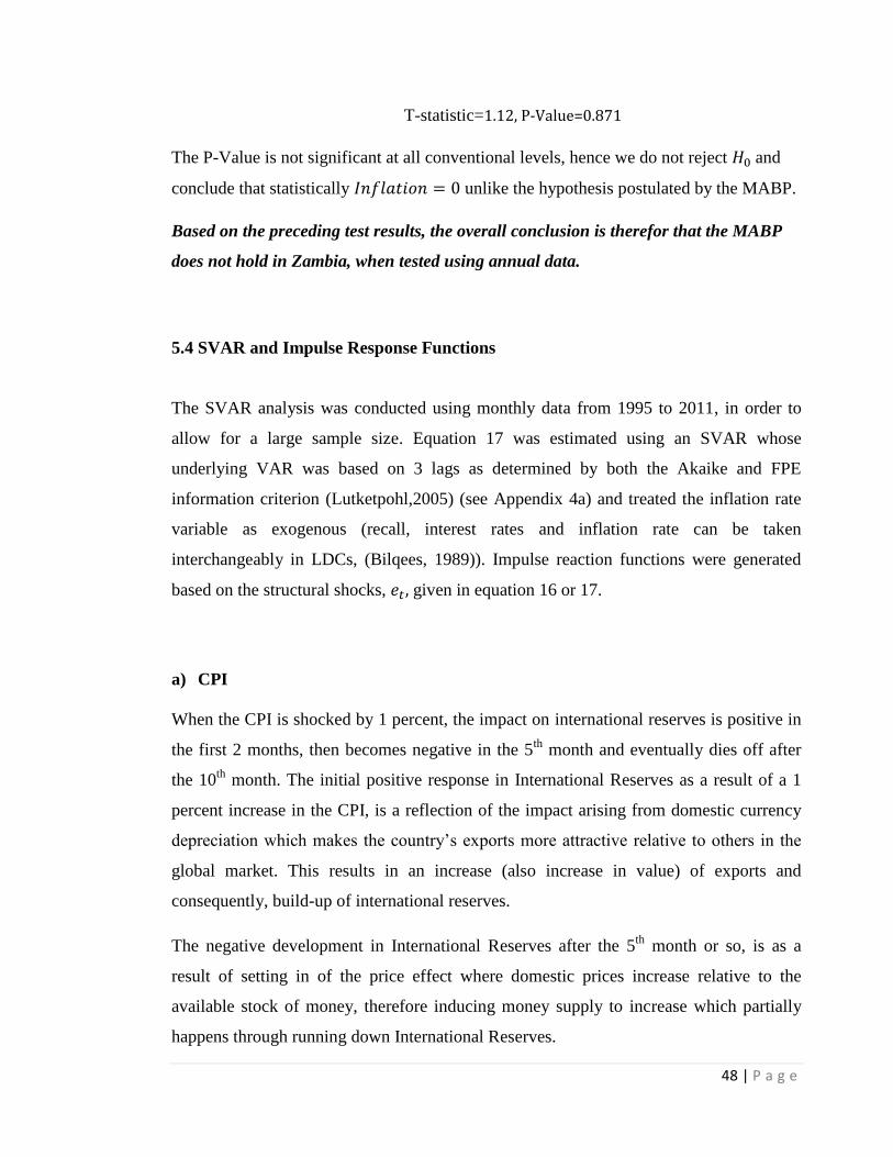
48 | P a g e
T-statistic=1.12, P-Value=0.871
The P-Value is not significant at all conventional levels, hence we do not reject and
conclude that statistically unlike the hypothesis postulated by the MABP.
Based on the preceding test results, the overall conclusion is therefor that the MABP
does not hold in Zambia, when tested using annual data.
5.4 SVAR and Impulse Response Functions
The SVAR analysis was conducted using monthly data from 1995 to 2011, in order to
allow for a large sample size. Equation 17 was estimated using an SVAR whose
underlying VAR was based on 3 lags as determined by both the Akaike and FPE
information criterion (Lutketpohl,2005) (see Appendix 4a) and treated the inflation rate
variable as exogenous (recall, interest rates and inflation rate can be taken
interchangeably in LDCs, (Bilqees, 1989)). Impulse reaction functions were generated
based on the structural shocks, given in equation 16 or 17.
a) CPI
When the CPI is shocked by 1 percent, the impact on international reserves is positive in
the first 2 months, then becomes negative in the 5th
month and eventually dies off after
the 10th
month. The initial positive response in International Reserves as a result of a 1
percent increase in the CPI, is a reflection of the impact arising from domestic currency
depreciation which makes the country’s exports more attractive relative to others in the
global market. This results in an increase (also increase in value) of exports and
consequently, build-up of international reserves.
The negative development in International Reserves after the 5th
month or so, is as a
result of setting in of the price effect where domestic prices increase relative to the
available stock of money, therefore inducing money supply to increase which partially
happens through running down International Reserves.
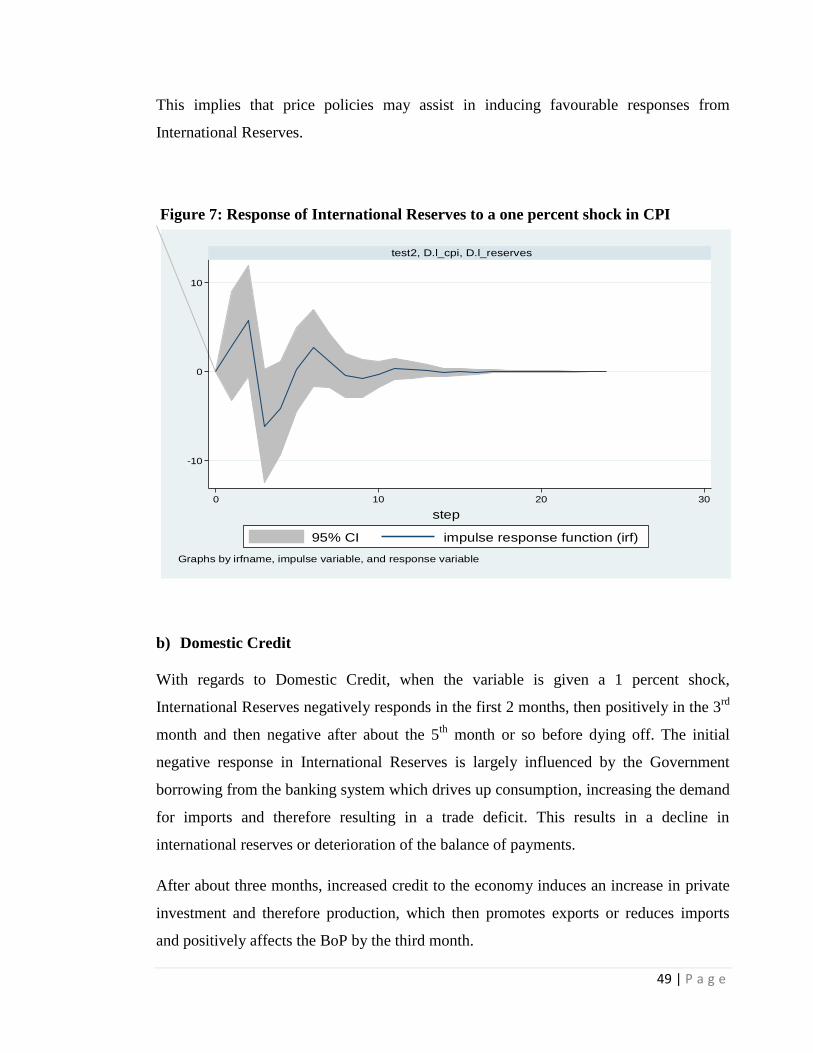
49 | P a g e
This implies that price policies may assist in inducing favourable responses from
International Reserves.
Figure 7: Response of International Reserves to a one percent shock in CPI
b) Domestic Credit
With regards to Domestic Credit, when the variable is given a 1 percent shock,
International Reserves negatively responds in the first 2 months, then positively in the 3rd
month and then negative after about the 5th
month or so before dying off. The initial
negative response in International Reserves is largely influenced by the Government
borrowing from the banking system which drives up consumption, increasing the demand
for imports and therefore resulting in a trade deficit. This results in a decline in
international reserves or deterioration of the balance of payments.
After about three months, increased credit to the economy induces an increase in private
investment and therefore production, which then promotes exports or reduces imports
and positively affects the BoP by the third month.
-10
0
10
0 10 20 30
test2, D.l_cpi, D.l_reserves
95% CI impulse response function (irf)
step
Graphs by irfname, impulse variable, and response variable
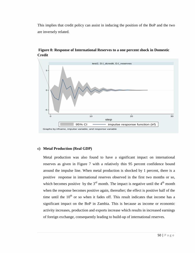
50 | P a g e
This implies that credit policy can assist in inducing the position of the BoP and the two
are inversely related.
Figure 8: Response of International Reserves to a one percent shock in Domestic
Credit
c) Metal Production (Real GDP)
Metal production was also found to have a significant impact on international
reserves as given in Figure 7 with a relatively thin 95 percent confidence bound
around the impulse line. When metal production is shocked by 1 percent, there is a
positive response in international reserves observed in the first two months or so,
which becomes positive by the 3rd
month. The impact is negative until the 4th
month
when the response becomes positive again, thereafter; the effect is positive half of the
time until the 10th
or so when it fades off. This result indicates that income has a
significant impact on the BoP in Zambia. This is because as income or economic
activity increases, production and exports increase which results in increased earnings
of foreign exchange, consequently leading to build-up of international reserves.
-5
0
5
0 10 20 30
test2, D.l_dcredit, D.l_reserves
95% CI impulse response function (irf)
step
Graphs by irfname, impulse variable, and response variable

51 | P a g e
Figure 9: Response of International Reserves to a one percent shock in Metal
Production (Real GDP)
d) The Money Multiplier
Similar to metal production (income), the money multiplier is found to have little impact
on International Reserves (BoP), with observes wide regions of the 95 percent confidence
bound around te impulse line (See Figure 7). The multiplier is observed to have an
insignificant impact on the BoP in the first 10 months or so which fades off afterwards.
-5
0
5
0 10 20 30
test2, D.l_metprxn, D.l_reserves
95% CI impulse response function (irf)
step
Graphs by irfname, impulse variable, and response variable
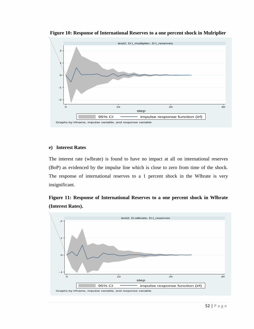
52 | P a g e
Figure 10: Response of International Reserves to a one percent shock in Mulriplier
e) Interest Rates
The interest rate (wlbrate) is found to have no impact at all on international reserves
(BoP) as evidenced by the impulse line which is close to zero from time of the shock.
The response of international reserves to a 1 percent shock in the Wlbrate is very
insignificant.
Figure 11: Response of International Reserves to a one percent shock in Wlbrate
(Interest Rates).
-2
-1
0
1
2
0 10 20 30
test2, D.l_multiplier, D.l_reserves
95% CI impulse response function (irf)
step
Graphs by irfname, impulse variable, and response variable
-.1
0
.1
.2
0 10 20 30
test2, D.wlbrate, D.l_reserves
95% CI impulse response function (irf)
step
Graphs by irfname, impulse variable, and response variable
53 | P a g e
5.6 Discussion
The research has first of all tested the applicability of the MABP in Zambia using the
OLS regression of the Reserve Flow Equation (RFE) for both monthly and annual data
during the 1980 to 2011 period when Zambia was actively pursuing the IMF support
programs for BoP problems. In both regressions, it is established that the conditions
provided by the MABP theory do not jointly hold in Zambia. The joint F-test of the null
hypothesis that constant =0, CPI =1, and multiplier=Domestic Credit = -1, do not hold at
all conventional levels of significance. In addition, the hypothesis that GDP >0, inflation
and interest rates<0 do not hold in monthly data as all the coefficients on these variables
are not significant at all conventional levels and the results are the same in annual data.
These results indicate that the MABP does not hold in Zambia.
Nevertheless, in the monthly regression it is revealed that CPI and Domestic Credit are
highly significant in influencing the BoP in Zambia. In particular, a 1 percent increase in
the growth of the CPI was found to induce a 1.32 percent increase in the rate of growth of
International Reserves, while a 1 percent rise in the growth of Domestic Credit was
estimated to lead to a 1.03 percent reduction in the growth of International Reserves. This
is similar to findings by Duasa (2007) who established that there was long-run
relationship between the Malaysian trade balance and monetary variables particularly,
prices and domestic credit. Further, in the regression using monthly data, the Money
Multiplier was found to be significant at a 5 percent level of significance, although the
negative sign of the coefficient contradicted a priori expectation. The rest of the variables
were insignificant.
Results from the regression using annual data were largely in line with those in the one
based on monthly data. Again, the CPI and Domestic Credit were observed to be highly
significant repressors. A 1 percent rise in the rate of growth of the CPI was found to
result in a 0.55 rise in the growth of International Reserves, where as a 1 percent increase
in the growth of Domestic Credit was revealed to induce a 1.03 percent reduction in the
rate of growth of International Reserves. The constant was also significant at a 5 percent
level of significance and the rest of the variables were insignificant. The regression

54 | P a g e
findings suggest that key influencing monetary variables for Zambia’s BoP are the CPI
and Domestic Credit. This implies that as far as monetary policy is concerned policies
around these two variables are more effective in influencing positive performance of
Zambia’ BoP.
Reinforcing the regression findings are the long run and short run estimations conducted
using the SVARs which indicated that three variables particularly, CPI, Domestic Credit
and Income have significant influence on International Reserves in Zambia. This is in
line with findings by Silumbu (1995) and Dhiliwayo (1996) who employed approaches
similar to the one used by this study and established that Domestic Credit and Inflation
hold significant effect on the balance of payments for Malawi and Zimbabwe
respectively.
The largest significant impact on International Reserves (or BoP) in Zambia is exerted by
CPI whose 1 percent shock has a positive impact in the first two months or so. The
response thereafter becomes negative from about 5 months and dies off after the 10th
month or so. The positive influence that 1 percent shock in CPI imposes on the BoP, is as
a result of the Kwacha depreciation relative to other currencies (exchange rate effect) that
is experienced as the price level increases. This depreciation makes local products more
attractive and more valuable on the international market which results in increased
earnings of foreign exchange from exports. By the 5th
month or so, the response of
international reserves becomes negative due to the price effect that sets in after inflation
as when domestic prices increase, residents resort to imported commodities which
increases the volumes of imports and exerts pressure on international reserves. The
reaction fades off after the 10th
step indicating that there is no long-run relationship
between CPI and international reserves.
A 1 percent shock in Domestic Credit has a significant negative impact on International
Reserves in the first 2 months which becomes positive after 5 months or so, then is
negative after 7 months and fades off after the 11th
month. The negative initial impulse in
International Reserves is an indication of increased consumption as credit increases,
which leads to the rise in imports thereby negatively affecting the trade balance.
Increased consumption in the initial stage reflects the significant participation of
55 | P a g e
Government in the borrowing market which crowds out private borrowing and
consequently adversely affects private investment. Part of the credit would have initially
gone to the private sector which eventually increases investment and production which
favourably affects the BoP, consequently resulting in the positive impact on the BoP in
the 5th
month.
The impulse reaction function results from the conducted SVAR reveals that Income
level or GDP does have a significant impact on International Reserves. This result is not
surprising, because as income levels increase, there is both increased local production
increased consumption which induce rises in exports and imports, which positively and
negatively respectively impact the BoP. The initial effect of a 1 percent shock on income
has a positive effect on the BoP largely through the trade balance as local production and
therefore exports increases. By the second month or so, the income shock also leads to
increased consumption which results in a rise imports, thereby negatively affecting the
BoP. The effects of the shock keep alternating in this manner until about the 10th
month
or so when it fades off.
The Interest Rate was also found to have no significant impact on the BoP in Zambia.
This is attributed to the fact that a rise in interest rate may have a double impact on the
BoP largely through the trade balance. High interest rates discourage borrowing and
therefore negatively affect output and exports while at the same time, high interest rates
will discourage consumption and possibly imports, therefore resulting in a neutral impact
on the external position.
Further, the impulse reaction function results indicate that the Money Multiplier does not
have significant impact on international reserves through the MABP channel. Changes in
the Money Multiplier induce changes in the money supply with the transmission of the
impacts continuing to other variables including interest rates, prices and output.
However, changes in the money multiplier have a double impact on the BoP transmitted
through the trade account just like in the case of interest rates. The resultant effect of a
shock in the Money Multiplier is neutral effect on the BoP.
56 | P a g e
CHAPETR 6
POLICY IMPLICATIONS AND CONCLUSION
The study successfully tested the MABP in Zambia for the period that the country was
actively receiving technical support on the BoP from the IMF and established that the
model does not hold implying that Zambia’s BoP is not purely a monetary phenomenon.
This is similar to findings by studies from other LDCs including Malawi (Silumbu 1995),
Nigeria (Bobai, 2013) and Zimbabwe (Dhiliwayo, 1996). In addition, Gulzar (2008) had
similar findings using Pakistan data.
Notwithstanding, it was established that the domestic price level and Domestic Credit
have highly significant effects on the BoP in Zambia. In this regard, the study suggests
that policy makers can work towards stabilising inflation as a way of maintaining a
balanced BoP. Changes in inflation exert both an exchange rate and price effect on the
domestic economy which impose turbulences in the overall BoP. However, stabilising
the price level is often a challenge as the variable is vulnerable to many other economic
phenomena both in the domestic and external environment that may lie outside the
control of monetary authorities.
Further, Domestic Credit whose impact on the BoP is negative reflecting a large
proportion of credit going to consumption, offers the best opportunity for monetary
authorities to influence the BoP as they have reasonably high control over the variable.
The study results indicate that if properly managed, domestic credit can be utilised to
turnaround the negative impact it may exert on the BoP to a positive one. Economic
prudence requires that most of the credit goes towards production especially that related
to non-traditional exports (NTEs) rather than consumption. Therefore, monetary
authorities in Zambia can take advantage of this by designing deliberate policy that
directs more credit towards the private sector, particularly industry involved in the
production of NTEs, which will result in a positive impact on the BoP. In addition, the
Government can also reduce its borrowing from the banking system to avoid crowding
out of the private sector, which will go a long way towards maintaining a healthy BoP.
57 | P a g e
Furthermore, following the finding that Income (GDP) also has a significant impact on
the BoP, the study recommends that policy makers should encourage growth policy
biased towards export oriented sectors, especially NTEs. The increased production
(activity) that may arise from increased incomes may lead to increased exports thus
posing a positive impact on the BoP. This could be used together with the interest rate
which can be a tool for inducing output and exports by promoting policy that offers lower
interest rates to producers of NTEs. In this regard, the Bank of Zambia may further
lower the policy rate in order to induce lower market interest rates and also promote
lending to the private sector involved in NTEs, in efforts to spur output and therefore
increase the country’s share on the international market and positively affect the BoP.
58 | P a g e
REFERENCES
Adamu, P. A. & Itsede, C. O. (2009). “Balance of adjustments: the West Africa
Monetary zone experience”. Journal of Monetary and Economic Integration.Vol.10 No.
2.
Aghevli, B. B. & Khan, M. S. (1977). The Monetary Approach to Balance of Payments
Determination: An empirical text. In International Monetary Fund (Eds.). The monetary
approach to the balance of payments. Washington, DC:
Alexander, S.S. 1952. "Effects of devaluation on a trade balance". IMF Staff Papers.
2(2):263-78.
Bank of Zambia, Annual Report 2010.
Bank of Zambia, Annual Report 2011.
Bank of Zambia, Annual Report 2012.
Bank of Zambia, Fortnightly Statistical Bulletin, (1995 to 2011)
Bank of Zambia, Jubilee Celebrations Booklet 2014.
Barbone, L. and F. Rivera-Batiz. 1987. "Foreign capital and contractionary impact of
currency devaluation, with application to Jamaica". Journal of Development
Economics. 26:1-15.
Bevan, D., P. Collier and P. Horsnell, 1990, Controlled Open Economies: A Neoclassical
Approach to Structuralism, Clarendon Press, Oxford.
Bilquees, F. (1989). “Monetary Approach to Balance of Paymens: The Evidence on
Reserve Flow from Pakistan.” The Pakistan Developmemt Review 28:3 (Autumn 1989)
195-206.

59 | P a g e
Blackwell, Carl P., 1978, 'Reflections on the Monetary Approach to the Balance of
Payments', IMF Survey, February 20, pp. 52-55 and March 6, pp. 7 1-73.
Blades, D.W., 1972, 'Devaluation and the Direction of Malawi 's Import Trade', East
African Economic Review, Vol. 4, No. 1, June, pp. 63-70.
Bobai, F. D. (2013). “An Empirical Analysis of the Balance of Payments as a Monetary
Phenomenon: Nigeria’s Experience.” Journal of Emerging Issues in Economics, Finance
and Banking, Vol. 1, No. 2.
Boateng, C. and Ayentimi, D. T. (2013). “An Empirical Analysis of Balance of Payment
in Ghana using the Monetary Approach.” European Journal of Business and
Management, Vol. 5, No. 8.
Breusch, T. S. (1978). “Testing for autocorrelation in dynamic linear models”. Australian
Economic Papers 17: 334–355.
Caves, R.E., J.A. Frankel, and R.W. Jones, 1990, World Trade and Payments, Scott,
Foresman/Little Brown Higher Education, Gensview.
Central Statistics Office, Monthly Statistical Bulletins (1995 to 2012).
Central Statistics Office, (2010). “Living Conditions Monitoring Survey.” CSO Zambia.
Chacholiades, M. (1990). International Economics. New York: McGraw-Hill Publishers.
Chaudhary, M.A. and Shabbir, G. (2004). “The Impact of Domestic Credit, Deficit and
Changing Exchange Rate Regimes on Foreign Reserves in Pakistan”. Pakistan Economic
and Social Review. 42 (1&2): 1-20.

60 | P a g e
Cheng, Hang-Sheng and Nicholas P. Sargen, 1975, 'Central-Bank Policy Towards
Inflation', Federal Reserve Bank of San Francisco Business Review, Spring, pp. 3 1-40.
Connolly, Michael and Dean Taylor, 1976, 'Testing the Monetary Approach to
Devaluation in Developing Countries', Journal of Political Economy, Vol. 84, pp. 849-
859.
Cooper, R., 1971, 'Currency Devaluation in Developing Countries' ,Essays in
International Finance, University Press, Princeton.
Coppin, A. (1994). “The Determinants of International Reserves in Barbados: A test of
the Monetarist Approach”.Journal of Social and Economic Studies, Vol. 43, No. 2,
pp.75–89.
Davidson, R., and MacKinnon J. G. (1993). “Estimation and Inference in Econometrics”.
New York: Oxford University Press.
Dhliwayo, R. (1996). “The Balance of Payments as a Monetary Phenomenon: An
Econometric Study of Zimbabwe’s Experience”. African Economic Research
Consortium, Research Paper 46.
Dhliwayo, R. and T. Moyo. 1990. "The Monetary Approach to Balance Of Payments: a
case study of Zimbabwe". Final Report. African Economic Research Consortium.
Nairobi.
Duasa, J. (2007). “Determinants of the Malaysian Trade Balance: An ARDL Bound
Testing Aproach”. Journal of Economic Co-operation 28 (3): 21-40.
61 | P a g e
Durbin, J. and G. S. Watson, (1950). Testing for serial correlation in least squares
regression”. I. Biometrika 37: 409–428.. 1951. Testing for serial correlation in least
squares regression. II. Biometrika 38: 159–177.
Durbin, J. (1970). “Testing for serial correlation in least-squares regressions when some
of the regressors are lagged dependent variables”. Econometrica 38: 410–421.
Dornbush, R. 1973. "Currency depreciation, hoarding and relative prices," Journal of
Political Economy. 81(4):893-915.
Enders, W., 2003. Applied Econometric Time Series. New York: John Wiley &
Sons, Inc.
Fleermuys, F. N. (2005). “The Balance of Payments as a Monetary Phenomenon: An
Econometric Study of Namibia”. DEA Research Discussion Paper No.72.
Gould,W.W. (1996). “Wald test of nonlinear hypotheses after model estimation”. Stata
Technical Balletin 29:2-4. College Station. TX: Stata Press.
Gulzar, A. (2008).”Pakistan’s Balance of Payments as a Monetary Phenomenon:
(Econometric Evidence)”. Journal of Managerial Sciences, 5(2):167-178.
Greene,W.H. (2012): “Econometric Analysis.” Seventh Edition, Upper Suddle Rirre,NJ:
Prentice Hall.
Howard, M. & Mamingi, N. (2002). “The Monetary Approach to the Balance of
Payments: An Application to Barbados”. The Singapore Economic Review, 47(2):213–
228.
62 | P a g e
International Monetary Fund, (1977). The monetary approach to balance of payments.
International Monetary Fund. Washington DC.
International Monetary Fund (1992). “IMF Conditionality 1980-1991”. Arlington, VA:
Alexis de Tocqueville Institution.
International Monetary Fund (1997):”Zambia - Selected Issues Statistical
Appendix”.Washington D.C.:International Monetary Fund.
International Monetary Fund, 2000: The IMF Approach to Economic Stabilization,
NBER Macroeconomics Annual 1999, Volume 14, MIT Press.
Inoue, T. and Hamori, S. (2009). “What Explains Real and Nominal Exchange Rate
Fluctuations? Evidence from SVAR Analysis for India.” IDE Discussion Paper No. 216.
Kannan, R. 1989. "Monetary approach to balance of payments- a case study of India,
1968-1985". Economic and Political Weekly. 15(4):627-636.
Kreinin, M.E. and Officer, L.H. 1978. "The monetary approach to balance of payments:
a survey". Study in International Finance. No. 43. Princeton University. Princeton.
Kremers, J.J.M. N.R. Eriscsson. and J.J. Dolado. 1992. "The power of cointegration
tests". Oxford Bulletin of Economics and Statistics. 54:325-48.
Lutkepohl, H. (2005). “New Introduction to Multiple Time Series Analysis”. New York:
Springer.

63 | P a g e
Machlup, F. 1955. "Relative prices and aggregate spending in the analysis of
devaluation". The American Economic Review. 45(3):255-78.
Magee, S.P. 1976. "The empirical evidence of the monetary approach to the balance of
payments and exchange rates". The American Economic Review. 66:163-70.
Miles, A.M. 1979. "The effects of devaluation on the trade balance and the balance of
payments". Journal of Political Economy. 87(3):600-19.
Miller, C. N. (1986). “A General Approach to the Balance of Payments and Exchange
Rates”. Journal of Economic Integration. 1(1):85-122.
Mishkin, F. (2004): “The Economics of Money, Banking and Financial Markets.”
Seventh Edition. Pearson.
Mundell, R.A. 1968. "International Economics". Macmillan. London.
Ranis, G. ed. 1971. "Government and Economic Development". Yale University. New
Haven.
Mutale, O. H. (1983): “Money Supply, Inflation and the Balance of Payments, Zambia
(1970-1980).” Master of Arts in Economics Dissertation, University of Zamabia.
Obioma, E. C. (1998). “Balance of Payments and Exchange Rate Management in
Nigeria: Empirical Evidence from the Monetary Approach”. NCEMA Policy Analysis
Series. 4 (2).
Ogiogio, G. O. (1996). “Exchange Rate Policy, Trade Policy Reform and the Balance of
Payments”.
Phillips, P. C. B. (1988). “The ET Interview: Professor James Durbin”. Econometric
Theory 4: 125–157.
64 | P a g e
Ravnik, R. and Zilic, I. (2010). “The use of SVAR Analysis in Determining the effects of
Fiscal Shocks in Croatia.”
Rivera-Batiz, F. and Rivera-Batiz, L. (1985). “International Finance and Open Economy
Macroeconomics”. MacMillan Publishing Company, New York.
Rosensweig, J.A. and E.W. Tallman. 1993. "Fiscal policy and trade adjustment: are the
deficits really twins?" Economic Inquiry. 31 (4):580-94.
Silumbu, E. B. D. (1995). “The role of Exchange Rate and Monetary Policy in the
Monetary Approach to the Balance of Payments: Evidence from Malawi.” Economic
Research Consortium, research paper 37.
Szeftel, M. (2000) “Eat With Us”: Managing Corruption and Patronage Under Zambia's
Three Republics, 1964-99. Journal of Contemporary African Studies, 18 (2), 207-224.
Taylor, Mark P., 1987, 'Testing the Exogeneity Specification underlying the Monetary
Approach to the Balance of Payments: Some UK Evidence', Applied Economics,
Vol. 19, No. 5, May, pp. 557-661.
The World Bank (2004) Zambia Country Economic Memorandum (In Two Volumes)
Umer, M., Muhammad, S. D., Abro, A. A., Sheikh, Q. A. & Ghazali, A. (2010). “Balance
of Payments as a Monetary Phenomenon: Econometric Evidence from Pakistan”,
International Research Journal of Finance and Economics, ISS 38.
Valinezhad, M. (1992). “A Comment on Lascaux’s Critique of the Monetary Approach
to the Balance of Payments”. Journal of Economic Issues, 26(1):262–270.
Whitman, Maria N., 1975, 'Global Monetarism and the Monetary Approach to the
Balance of Payments', Brookings Papers on Economic Activity, No. 3, pp. 491-536.

65 | P a g e
APPENDICES
Appendix 1: Unit Root Test Results
Table 7: Unit Root Test Results, Monthly Data
Variable Test Level: Z(t)[P-Value]
Logged Value: Z(t)[P-Value]
First Difference of Logged Value: Z(t)[P-Value]
Inter_Reserves ADF 0.255[0.9752] Weighted-4.240[0.0006]*** Weighted-19.649[0.000]***
Phillips-Perron 0.913[0.9933] Weighted-3.782[0.0031]*** Weighted-21.128[0.000]*** D_Credit ADF 0.565[0.9867] Weighted-4.795[0.0001]*** Weighted-19.502[0.000]***
Phillips-Perron 0.870[0.9927] Weighted-4.442-[0.003]*** Weighted-20.931[0.000]*** CPI ADF 0.555[0.9865] 1.903[0.3305] -12.786[0.000]***
Phillips-Perron 0.623[0.9882] -1.954[0.3069] -12.781[0.000]*** Met Production ADF -2.000 [0.2864] -3.158[0.0225]** -23.158[0.000]***
Phillips-Perron 0.768 [0.8285] -2.107[0.2416] -23.489[0.000]*** Wlbrate ADF 1.590[0.4884] -1.205[0.6714] not logged-15.246[0.000]***
Phillips-Perron -1.245[0.6541] -0.898[0.7888] not logged-15.819[0.000]*** Multipler ADF -4.444[0.0002]*** -5.444[0.000]*** -22.059[0.000]***
Phillips-Perron -4.438[0.0003]*** -5.774[0.000]*** -26.972[0.000]*** Inflation ADF -2.837[0.0535]* -2.386[0.1457] not logged-14.223[0.000]***
Phillips-Perron -2.587[0.0957]* -2.045[0.2674] not logged-14.497[0.000]***
Recall: ADF is Augmented Dickey-Fuller Test. The null hypotheses for all the tests are that
there is a unit root (i.e. the variable is non-stationary); (***) implies significance at 1 percent, 5
percent and 10 percent, (**) significance at 5 percent and 10 percent and (*) significance at 10
percent only.
Table 8: Unit Root Test Results, Annual Data
Variable Test Level:
Z(t)[P-Value]
Logged Value:
Z(t)[P-Value]
First Difference of Logged Value;
Z(t)[P-Value]
Inter_Reserves ADF 4.1489[0.000]*** Weighted (2.502)[0.1151] Weighted (8.023)[0.0000]***
Phillips-Perron 5.873[0.000]*** Weighted (2.390)[0.1446] Weighted (8.615)[0.0000]*** D_Credit ADF 5.818[0.000]*** Weighted(4.473[0.0002]*** Weighted (7.966)[0.0000]***
Phillips-Perron 7.451[0.000]*** Weighted (4.4441)[0.0003]*** Weighted (8.619)[0.0000]*** CPI ADF 11.115[0.000]*** (2.087)[0.2497) (1.665)[0.4490]
Phillips-Perron 7.092[0.000]*** (1.444)[0.5609] (1.695)[0.4336] GDP ADF 3.849[0.000]*** 2.180[0.9989] (5.397)[0.0000]***
Phillips-Perron 5.184[0.000]*** 3.134[1.000]*** (5.438)[0.0000]*** BoZrate ADF (1.986)[0.292] (1.646)[0.4589] not logged (6.545)[0.0000]***
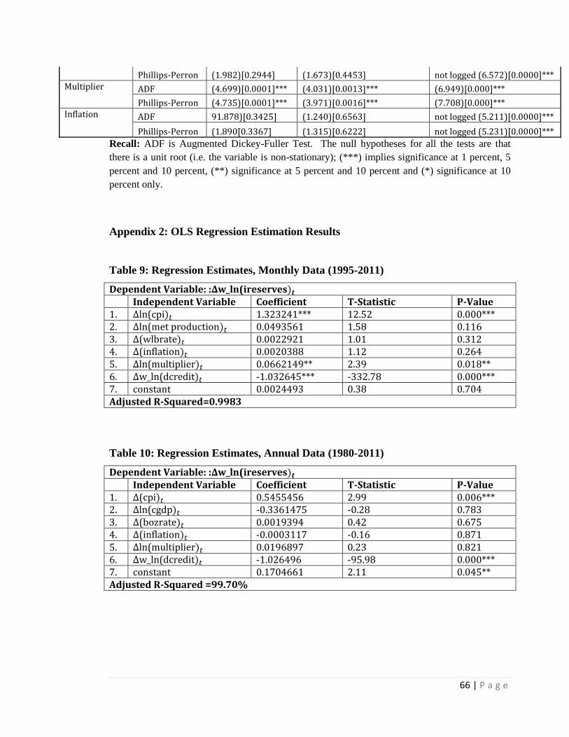
66 | P a g e
Phillips-Perron (1.982)[0.2944] (1.673)[0.4453] not logged (6.572)[0.0000]*** Multiplier ADF (4.699)[0.0001]*** (4.031)[0.0013]*** (6.949)[0.000]***
Phillips-Perron (4.735)[0.0001]*** (3.971)[0.0016]*** (7.708)[0.000]*** Inflation ADF 91.878)[0.3425] (1.240)[0.6563] not logged (5.211)[0.0000]***
Phillips-Perron (1.890[0.3367] (1.315)[0.6222] not logged (5.231)[0.0000]***
Recall: ADF is Augmented Dickey-Fuller Test. The null hypotheses for all the tests are that
there is a unit root (i.e. the variable is non-stationary); (***) implies significance at 1 percent, 5
percent and 10 percent, (**) significance at 5 percent and 10 percent and (*) significance at 10
percent only.
Appendix 2: OLS Regression Estimation Results
Table 9: Regression Estimates, Monthly Data (1995-2011)
Dependent Variable: :∆w_ln(ireserves Independent Variable Coefficient T-Statistic P-Value 1. ∆ln(cpi 1.323241*** 12.52 0.000*** 2. ∆ln(met production 0.0493561 1.58 0.116 3. ∆(wlbrate 0.0022921 1.01 0.312 4. ∆(inflation 0.0020388 1.12 0.264 5. ∆ln(multiplier 0.0662149** 2.39 0.018** 6. ∆w_ln(dcredit -1.032645*** -332.78 0.000*** 7. constant 0.0024493 0.38 0.704 Adjusted R-Squared=0.9983
Table 10: Regression Estimates, Annual Data (1980-2011)
Dependent Variable: :∆w_ln(ireserves Independent Variable Coefficient T-Statistic P-Value 1. ∆(cpi 0.5455456 2.99 0.006*** 2. ∆ln(cgdp -0.3361475 -0.28 0.783 3. ∆(bozrate 0.0019394 0.42 0.675 4. ∆(inflation -0.0003117 -0.16 0.871 5. ∆ln(multiplier 0.0196897 0.23 0.821 6. ∆w_ln(dcredit -1.026496 -95.98 0.000*** 7. constant 0.1704661 2.11 0.045** Adjusted R-Squared =99.70%

67 | P a g e
Appendix 3: OLS Post Regression Diagnostic Tests
Table 11: Summary of post regression diagnostic tests results
Test Monthly Data
Annual Data
H0:there is Conclusion
Breush-Pagan/ Cook-Weisberg (P-Value)
0.3034 0.227 Heteroscedesticity There is Homostedasticity in all models
Vif 1.06 1.82 There is Multicollinearity
There is no Multicollinearity in both models
Durbin-Watson (d-statistic)
2.2354≈2 2.2784≈2 No Serial Correlation
There is no serial correlation in both models
Dickey-Fuller Predicted Residuals (P-Value)
0.0000*** 0.0000*** Unit root in predicted redsiduals
There is no Unit root in the predicted residuals
Following the above positive result of the post estimation diagnostics, it was concluded
that the estimations based on both monthly and annual data were statistically valid to be
used for inference.
Appendix 4: VAR Outputs
a) Lag-order selection
Exogenous: D.inflationrates _cons D.l_dcredit Endogenous: D.l_reserves D.l_cpi D.l_metprxn D.wlbrate D.l_multiplier 4 -82.4013 61.362* 36 0.005 4.5e-07 2.39599 3.44087 4.97768 3 -113.082 128.26 36 0.000 4.2e-07* 2.34253* 3.14628 4.32845 2 -177.213 88.733 36 0.000 5.6e-07 2.62526 3.18789 4.0154 1 -221.58 140.69 36 0.000 6.1e-07 2.70935 3.03085* 3.50371 0 -291.925 8.5e-07 3.05452 3.13489 3.25311* lag LL LR df p FPE AIC HQIC SBIC Sample: 1960m7 - 1977m1 Number of obs = 199 Selection-order criteria
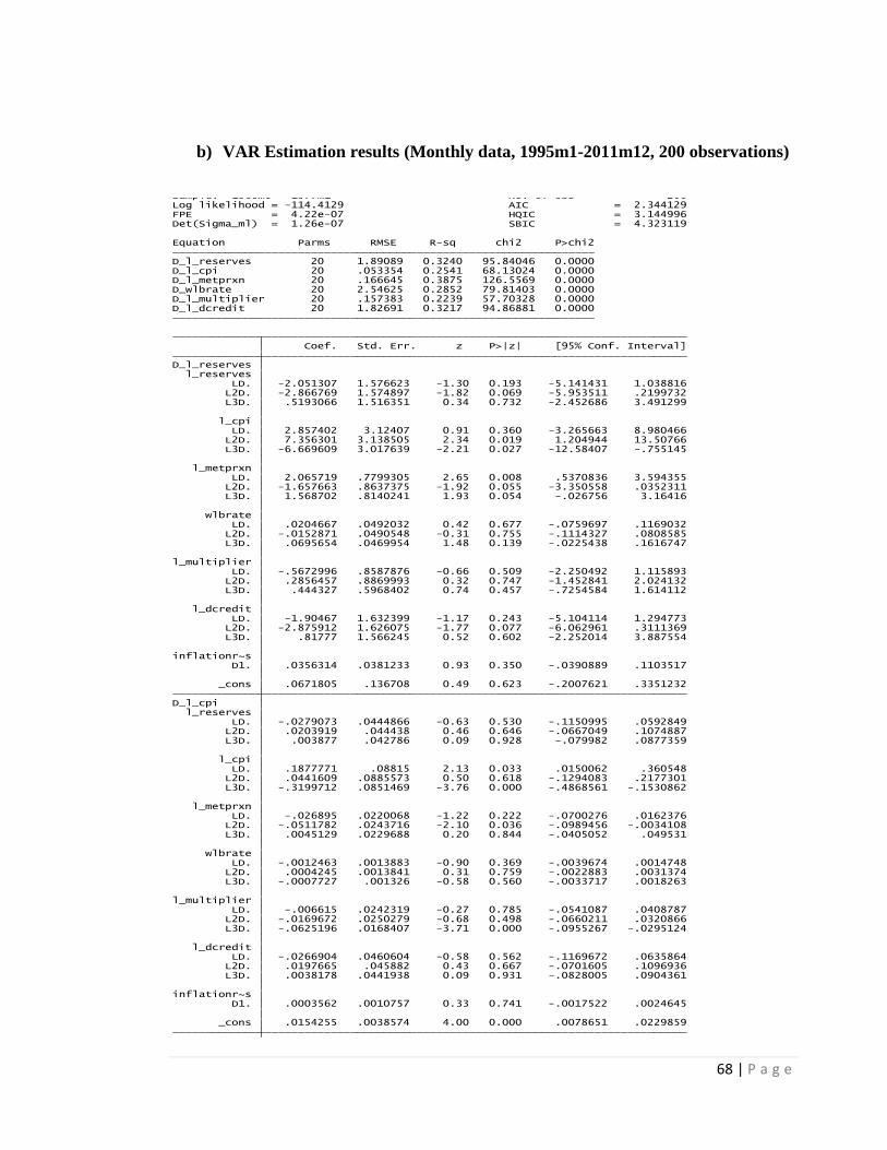
68 | P a g e
b) VAR Estimation results (Monthly data, 1995m1-2011m12, 200 observations)
_cons .0154255 .0038574 4.00 0.000 .0078651 .0229859 D1. .0003562 .0010757 0.33 0.741 -.0017522 .0024645inflationr~s L3D. .0038178 .0441938 0.09 0.931 -.0828005 .0904361 L2D. .0197665 .045882 0.43 0.667 -.0701605 .1096936 LD. -.0266904 .0460604 -0.58 0.562 -.1169672 .0635864 l_dcredit L3D. -.0625196 .0168407 -3.71 0.000 -.0955267 -.0295124 L2D. -.0169672 .0250279 -0.68 0.498 -.0660211 .0320866 LD. -.006615 .0242319 -0.27 0.785 -.0541087 .0408787l_multiplier L3D. -.0007727 .001326 -0.58 0.560 -.0033717 .0018263 L2D. .0004245 .0013841 0.31 0.759 -.0022883 .0031374 LD. -.0012463 .0013883 -0.90 0.369 -.0039674 .0014748 wlbrate L3D. .0045129 .0229688 0.20 0.844 -.0405052 .049531 L2D. -.0511782 .0243716 -2.10 0.036 -.0989456 -.0034108 LD. -.026895 .0220068 -1.22 0.222 -.0700276 .0162376 l_metprxn L3D. -.3199712 .0851469 -3.76 0.000 -.4868561 -.1530862 L2D. .0441609 .0885573 0.50 0.618 -.1294083 .2177301 LD. .1877771 .08815 2.13 0.033 .0150062 .360548 l_cpi L3D. .003877 .042786 0.09 0.928 -.079982 .0877359 L2D. .0203919 .044438 0.46 0.646 -.0667049 .1074887 LD. -.0279073 .0444866 -0.63 0.530 -.1150995 .0592849 l_reserves D_l_cpi _cons .0671805 .136708 0.49 0.623 -.2007621 .3351232 D1. .0356314 .0381233 0.93 0.350 -.0390889 .1103517inflationr~s L3D. .81777 1.566245 0.52 0.602 -2.252014 3.887554 L2D. -2.875912 1.626075 -1.77 0.077 -6.062961 .3111369 LD. -1.90467 1.632399 -1.17 0.243 -5.104114 1.294773 l_dcredit L3D. .444327 .5968402 0.74 0.457 -.7254584 1.614112 L2D. .2856457 .8869993 0.32 0.747 -1.452841 2.024132 LD. -.5672996 .8587876 -0.66 0.509 -2.250492 1.115893l_multiplier L3D. .0695654 .0469954 1.48 0.139 -.0225438 .1616747 L2D. -.0152871 .0490548 -0.31 0.755 -.1114327 .0808585 LD. .0204667 .0492032 0.42 0.677 -.0759697 .1169032 wlbrate L3D. 1.568702 .8140241 1.93 0.054 -.026756 3.16416 L2D. -1.657663 .8637375 -1.92 0.055 -3.350558 .0352311 LD. 2.065719 .7799305 2.65 0.008 .5370836 3.594355 l_metprxn L3D. -6.669609 3.017639 -2.21 0.027 -12.58407 -.755145 L2D. 7.356301 3.138505 2.34 0.019 1.204944 13.50766 LD. 2.857402 3.12407 0.91 0.360 -3.265663 8.980466 l_cpi L3D. .5193066 1.516351 0.34 0.732 -2.452686 3.491299 L2D. -2.866769 1.574897 -1.82 0.069 -5.953511 .2199732 LD. -2.051307 1.576623 -1.30 0.193 -5.141431 1.038816 l_reserves D_l_reserves Coef. Std. Err. z P>|z| [95% Conf. Interval]
D_l_dcredit 20 1.82691 0.3217 94.86881 0.0000D_l_multiplier 20 .157383 0.2239 57.70328 0.0000D_wlbrate 20 2.54625 0.2852 79.81403 0.0000D_l_metprxn 20 .166645 0.3875 126.5569 0.0000D_l_cpi 20 .053354 0.2541 68.13024 0.0000D_l_reserves 20 1.89089 0.3240 95.84046 0.0000 Equation Parms RMSE R-sq chi2 P>chi2
Det(Sigma_ml) = 1.26e-07 SBIC = 4.323119FPE = 4.22e-07 HQIC = 3.144996Log likelihood = -114.4129 AIC = 2.344129Sample: 1960m6 - 1977m1 No. of obs = 200
Vector autoregression
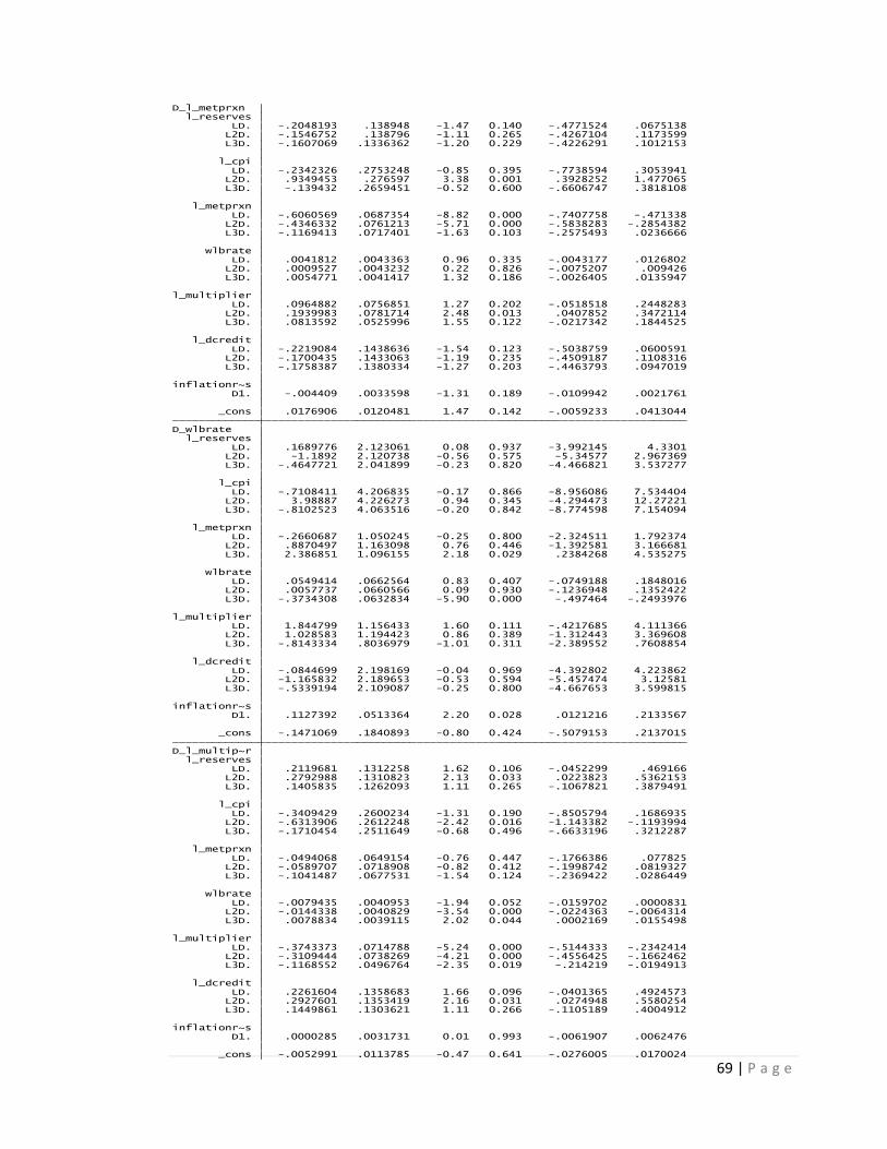
69 | P a g e
_cons -.0052991 .0113785 -0.47 0.641 -.0276005 .0170024 D1. .0000285 .0031731 0.01 0.993 -.0061907 .0062476inflationr~s L3D. .1449861 .1303621 1.11 0.266 -.1105189 .4004912 L2D. .2927601 .1353419 2.16 0.031 .0274948 .5580254 LD. .2261604 .1358683 1.66 0.096 -.0401365 .4924573 l_dcredit L3D. -.1168552 .0496764 -2.35 0.019 -.214219 -.0194913 L2D. -.3109444 .0738269 -4.21 0.000 -.4556425 -.1662462 LD. -.3743373 .0714788 -5.24 0.000 -.5144333 -.2342414l_multiplier L3D. .0078834 .0039115 2.02 0.044 .0002169 .0155498 L2D. -.0144338 .0040829 -3.54 0.000 -.0224363 -.0064314 LD. -.0079435 .0040953 -1.94 0.052 -.0159702 .0000831 wlbrate L3D. -.1041487 .0677531 -1.54 0.124 -.2369422 .0286449 L2D. -.0589707 .0718908 -0.82 0.412 -.1998742 .0819327 LD. -.0494068 .0649154 -0.76 0.447 -.1766386 .077825 l_metprxn L3D. -.1710454 .2511649 -0.68 0.496 -.6633196 .3212287 L2D. -.6313906 .2612248 -2.42 0.016 -1.143382 -.1193994 LD. -.3409429 .2600234 -1.31 0.190 -.8505794 .1686935 l_cpi L3D. .1405835 .1262093 1.11 0.265 -.1067821 .3879491 L2D. .2792988 .1310823 2.13 0.033 .0223823 .5362153 LD. .2119681 .1312258 1.62 0.106 -.0452299 .469166 l_reserves D_l_multip~r _cons -.1471069 .1840893 -0.80 0.424 -.5079153 .2137015 D1. .1127392 .0513364 2.20 0.028 .0121216 .2133567inflationr~s L3D. -.5339194 2.109087 -0.25 0.800 -4.667653 3.599815 L2D. -1.165832 2.189653 -0.53 0.594 -5.457474 3.12581 LD. -.0844699 2.198169 -0.04 0.969 -4.392802 4.223862 l_dcredit L3D. -.8143334 .8036979 -1.01 0.311 -2.389552 .7608854 L2D. 1.028583 1.194423 0.86 0.389 -1.312443 3.369608 LD. 1.844799 1.156433 1.60 0.111 -.4217685 4.111366l_multiplier L3D. -.3734308 .0632834 -5.90 0.000 -.497464 -.2493976 L2D. .0057737 .0660566 0.09 0.930 -.1236948 .1352422 LD. .0549414 .0662564 0.83 0.407 -.0749188 .1848016 wlbrate L3D. 2.386851 1.096155 2.18 0.029 .2384268 4.535275 L2D. .8870497 1.163098 0.76 0.446 -1.392581 3.166681 LD. -.2660687 1.050245 -0.25 0.800 -2.324511 1.792374 l_metprxn L3D. -.8102523 4.063516 -0.20 0.842 -8.774598 7.154094 L2D. 3.98887 4.226273 0.94 0.345 -4.294473 12.27221 LD. -.7108411 4.206835 -0.17 0.866 -8.956086 7.534404 l_cpi L3D. -.4647721 2.041899 -0.23 0.820 -4.466821 3.537277 L2D. -1.1892 2.120738 -0.56 0.575 -5.34577 2.967369 LD. .1689776 2.123061 0.08 0.937 -3.992145 4.3301 l_reserves D_wlbrate _cons .0176906 .0120481 1.47 0.142 -.0059233 .0413044 D1. -.004409 .0033598 -1.31 0.189 -.0109942 .0021761inflationr~s L3D. -.1758387 .1380334 -1.27 0.203 -.4463793 .0947019 L2D. -.1700435 .1433063 -1.19 0.235 -.4509187 .1108316 LD. -.2219084 .1438636 -1.54 0.123 -.5038759 .0600591 l_dcredit L3D. .0813592 .0525996 1.55 0.122 -.0217342 .1844525 L2D. .1939983 .0781714 2.48 0.013 .0407852 .3472114 LD. .0964882 .0756851 1.27 0.202 -.0518518 .2448283l_multiplier L3D. .0054771 .0041417 1.32 0.186 -.0026405 .0135947 L2D. .0009527 .0043232 0.22 0.826 -.0075207 .009426 LD. .0041812 .0043363 0.96 0.335 -.0043177 .0126802 wlbrate L3D. -.1169413 .0717401 -1.63 0.103 -.2575493 .0236666 L2D. -.4346332 .0761213 -5.71 0.000 -.5838283 -.2854382 LD. -.6060569 .0687354 -8.82 0.000 -.7407758 -.471338 l_metprxn L3D. -.139432 .2659451 -0.52 0.600 -.6606747 .3818108 L2D. .9349453 .276597 3.38 0.001 .3928252 1.477065 LD. -.2342326 .2753248 -0.85 0.395 -.7738594 .3053941 l_cpi L3D. -.1607069 .1336362 -1.20 0.229 -.4226291 .1012153 L2D. -.1546752 .138796 -1.11 0.265 -.4267104 .1173599 LD. -.2048193 .138948 -1.47 0.140 -.4771524 .0675138 l_reserves D_l_metprxn

70 | P a g e
Appendix 5: VAR Post Estimation Diagnostics
a) Granger Causality
_cons -.0384369 .1320821 -0.29 0.771 -.2973129 .2204392 D1. -.0321747 .0368333 -0.87 0.382 -.1043667 .0400172inflationr~s L3D. -1.021194 1.513247 -0.67 0.500 -3.987103 1.944715 L2D. 2.614226 1.571052 1.66 0.096 -.4649797 5.693432 LD. 1.517639 1.577162 0.96 0.336 -1.573542 4.60882 l_dcredit L3D. -.5380936 .5766444 -0.93 0.351 -1.668296 .5921088 L2D. -.2537142 .8569852 -0.30 0.767 -1.933374 1.425946 LD. .6607755 .8297281 0.80 0.426 -.9654617 2.287013l_multiplier L3D. -.0650626 .0454052 -1.43 0.152 -.1540551 .0239299 L2D. .0173354 .0473949 0.37 0.715 -.0755568 .1102276 LD. -.0213589 .0475383 -0.45 0.653 -.1145322 .0718143 wlbrate L3D. -1.544729 .7864792 -1.96 0.050 -3.0862 -.0032581 L2D. 1.554868 .8345105 1.86 0.062 -.0807421 3.190479 LD. -2.081201 .7535393 -2.76 0.006 -3.558111 -.6042909 l_metprxn L3D. 6.361704 2.915529 2.18 0.029 .6473728 12.07604 L2D. -6.923163 3.032305 -2.28 0.022 -12.86637 -.9799553 LD. -2.093446 3.018358 -0.69 0.488 -8.009319 3.822427 l_cpi L3D. -.7247859 1.46504 -0.49 0.621 -3.596212 2.146641 L2D. 2.616835 1.521606 1.72 0.085 -.3654583 5.599129 LD. 1.663613 1.523273 1.09 0.275 -1.321947 4.649174 l_reserves D_l_dcredit
D_l_dcredit ALL 41.73 15 0.000 D_l_dcredit D.l_multiplier 1.8497 3 0.604 D_l_dcredit D.wlbrate 2.3451 3 0.504 D_l_dcredit D.l_metprxn 31.199 3 0.000 D_l_dcredit D.l_cpi 10.178 3 0.017 D_l_dcredit D.l_reserves 4.5241 3 0.210 D_l_multiplier ALL 30.704 15 0.010 D_l_multiplier D.l_dcredit 6.1589 3 0.104 D_l_multiplier D.wlbrate 21.631 3 0.000 D_l_multiplier D.l_metprxn 2.4497 3 0.484 D_l_multiplier D.l_cpi 7.7165 3 0.052 D_l_multiplier D.l_reserves 5.9151 3 0.116 D_wlbrate ALL 18.031 15 0.261 D_wlbrate D.l_dcredit .30919 3 0.958 D_wlbrate D.l_multiplier 4.4361 3 0.218 D_wlbrate D.l_metprxn 5.7486 3 0.125 D_wlbrate D.l_cpi .96542 3 0.810 D_wlbrate D.l_reserves .38073 3 0.944 D_l_metprxn ALL 29.606 15 0.013 D_l_metprxn D.l_dcredit 3.8126 3 0.282 D_l_metprxn D.l_multiplier 7.3604 3 0.061 D_l_metprxn D.wlbrate 2.5187 3 0.472 D_l_metprxn D.l_cpi 12.634 3 0.005 D_l_metprxn D.l_reserves 3.426 3 0.330 D_l_cpi ALL 28.071 15 0.021 D_l_cpi D.l_dcredit .70384 3 0.872 D_l_cpi D.l_multiplier 13.837 3 0.003 D_l_cpi D.wlbrate 1.1767 3 0.759 D_l_cpi D.l_metprxn 6.6178 3 0.085 D_l_cpi D.l_reserves .82019 3 0.845 D_l_reserves ALL 41.636 15 0.000 D_l_reserves D.l_dcredit 4.8889 3 0.180 D_l_reserves D.l_multiplier 1.2848 3 0.733 D_l_reserves D.wlbrate 2.4179 3 0.490 D_l_reserves D.l_metprxn 30.558 3 0.000 D_l_reserves D.l_cpi 10.921 3 0.012 Equation Excluded chi2 df Prob > chi2 Granger causality Wald tests
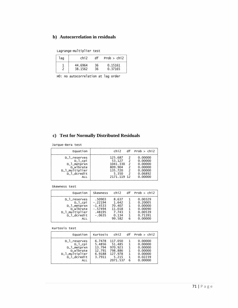
71 | P a g e
b) Autocorrelation in residuals
c) Test for Normally Distributed Residuals
H0: no autocorrelation at lag order 2 38.1562 36 0.37165 1 44.6964 36 0.15161 lag chi2 df Prob > chi2 Lagrange-multiplier test
ALL 2071.537 6 0.00000 D_l_dcredit 3.7911 5.215 1 0.02239 D_l_multiplier 6.9188 127.978 1 0.00000 D_wlbrate 12.791 798.886 1 0.00000 D_l_metprxn 13.794 970.923 1 0.00000 D_l_cpi 5.4856 51.485 1 0.00000 D_l_reserves 6.7478 117.050 1 0.00000 Equation Kurtosis chi2 df Prob > chi2 Kurtosis test
ALL 99.582 6 0.00000 D_l_dcredit -.0635 0.134 1 0.71391 D_l_multiplier .48195 7.743 1 0.00539 D_wlbrate -.57494 11.018 1 0.00090 D_l_metprxn -1.4533 70.407 1 0.00000 D_l_cpi -.22194 1.642 1 0.20005 D_l_reserves .50903 8.637 1 0.00329 Equation Skewness chi2 df Prob > chi2 Skewness test
ALL 2171.119 12 0.00000 D_l_dcredit 5.350 2 0.06892 D_l_multiplier 135.720 2 0.00000 D_wlbrate 809.904 2 0.00000 D_l_metprxn 1041.330 2 0.00000 D_l_cpi 53.127 2 0.00000 D_l_reserves 125.687 2 0.00000 Equation chi2 df Prob > chi2 Jarque-Bera test

72 | P a g e
d) Stability of Condition of Estimates
VAR satisfies stability condition. All the eigenvalues lie inside the unit circle. -.1352674 .135267 -.5803376 .580338 -.5723139 - .1320154i .587343 -.5723139 + .1320154i .587343 -.2130745 - .5584171i .597688 -.2130745 + .5584171i .597688 .1955638 - .566566i .599368 .1955638 + .566566i .599368 .3685901 - .4948176i .617011 .3685901 + .4948176i .617011 .04730609 - .6277224i .629502 .04730609 + .6277224i .629502 .3438828 - .6114582i .701524 .3438828 + .6114582i .701524 .314921 - .6360795i .709769 .314921 + .6360795i .709769 -.7627449 - .09282677i .768373 -.7627449 + .09282677i .768373 Eigenvalue Modulus Eigenvalue stability condition
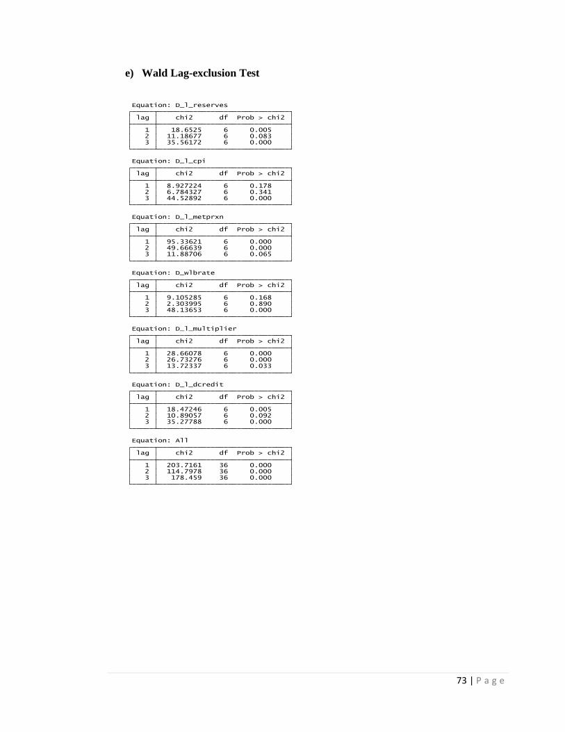
73 | P a g e
e) Wald Lag-exclusion Test
3 178.459 36 0.000 2 114.7978 36 0.000 1 203.7161 36 0.000 lag chi2 df Prob > chi2 Equation: All
3 35.27788 6 0.000 2 10.89057 6 0.092 1 18.47246 6 0.005 lag chi2 df Prob > chi2 Equation: D_l_dcredit
3 13.72337 6 0.033 2 26.73276 6 0.000 1 28.66078 6 0.000 lag chi2 df Prob > chi2 Equation: D_l_multiplier
3 48.13653 6 0.000 2 2.303995 6 0.890 1 9.105285 6 0.168 lag chi2 df Prob > chi2 Equation: D_wlbrate
3 11.88706 6 0.065 2 49.66639 6 0.000 1 95.33621 6 0.000 lag chi2 df Prob > chi2 Equation: D_l_metprxn
3 44.52892 6 0.000 2 6.784327 6 0.341 1 8.927224 6 0.178 lag chi2 df Prob > chi2 Equation: D_l_cpi
3 35.56172 6 0.000 2 11.18677 6 0.083 1 18.6525 6 0.005 lag chi2 df Prob > chi2 Equation: D_l_reserves
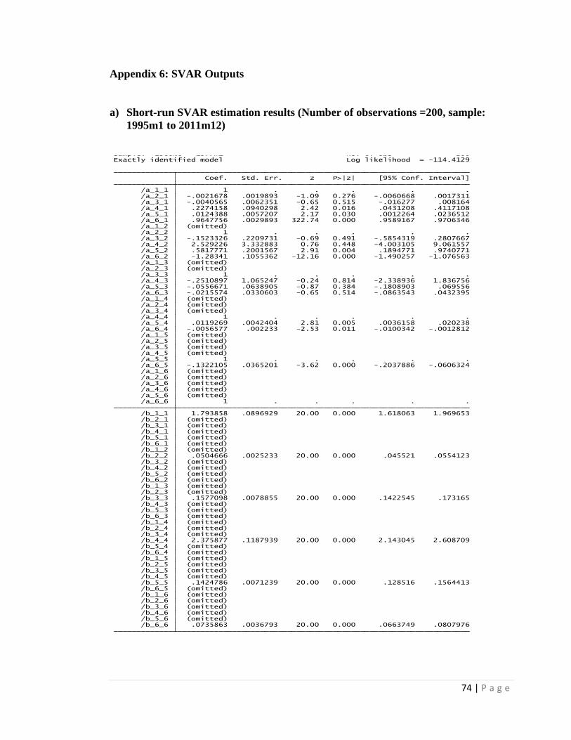
74 | P a g e
Appendix 6: SVAR Outputs
a) Short-run SVAR estimation results (Number of observations =200, sample:
1995m1 to 2011m12)
/b_6_6 .0735863 .0036793 20.00 0.000 .0663749 .0807976 /b_5_6 (omitted) /b_4_6 (omitted) /b_3_6 (omitted) /b_2_6 (omitted) /b_1_6 (omitted) /b_6_5 (omitted) /b_5_5 .1424786 .0071239 20.00 0.000 .128516 .1564413 /b_4_5 (omitted) /b_3_5 (omitted) /b_2_5 (omitted) /b_1_5 (omitted) /b_6_4 (omitted) /b_5_4 (omitted) /b_4_4 2.375877 .1187939 20.00 0.000 2.143045 2.608709 /b_3_4 (omitted) /b_2_4 (omitted) /b_1_4 (omitted) /b_6_3 (omitted) /b_5_3 (omitted) /b_4_3 (omitted) /b_3_3 .1577098 .0078855 20.00 0.000 .1422545 .173165 /b_2_3 (omitted) /b_1_3 (omitted) /b_6_2 (omitted) /b_5_2 (omitted) /b_4_2 (omitted) /b_3_2 (omitted) /b_2_2 .0504666 .0025233 20.00 0.000 .045521 .0554123 /b_1_2 (omitted) /b_6_1 (omitted) /b_5_1 (omitted) /b_4_1 (omitted) /b_3_1 (omitted) /b_2_1 (omitted) /b_1_1 1.793858 .0896929 20.00 0.000 1.618063 1.969653 /a_6_6 1 . . . . . /a_5_6 (omitted) /a_4_6 (omitted) /a_3_6 (omitted) /a_2_6 (omitted) /a_1_6 (omitted) /a_6_5 -.1322105 .0365201 -3.62 0.000 -.2037886 -.0606324 /a_5_5 1 . . . . . /a_4_5 (omitted) /a_3_5 (omitted) /a_2_5 (omitted) /a_1_5 (omitted) /a_6_4 -.0056577 .002233 -2.53 0.011 -.0100342 -.0012812 /a_5_4 .0119269 .0042404 2.81 0.005 .0036158 .020238 /a_4_4 1 . . . . . /a_3_4 (omitted) /a_2_4 (omitted) /a_1_4 (omitted) /a_6_3 -.0215574 .0330603 -0.65 0.514 -.0863543 .0432395 /a_5_3 -.0556671 .0638905 -0.87 0.384 -.1808903 .069556 /a_4_3 -.2510897 1.065247 -0.24 0.814 -2.338936 1.836756 /a_3_3 1 . . . . . /a_2_3 (omitted) /a_1_3 (omitted) /a_6_2 -1.28341 .1055362 -12.16 0.000 -1.490257 -1.076563 /a_5_2 .5817771 .2001567 2.91 0.004 .1894771 .9740771 /a_4_2 2.529226 3.332883 0.76 0.448 -4.003105 9.061557 /a_3_2 -.1523326 .2209731 -0.69 0.491 -.5854319 .2807667 /a_2_2 1 . . . . . /a_1_2 (omitted) /a_6_1 .9647756 .0029893 322.74 0.000 .9589167 .9706346 /a_5_1 .0124388 .0057207 2.17 0.030 .0012264 .0236512 /a_4_1 .2274158 .0940298 2.42 0.016 .0431208 .4117108 /a_3_1 -.0040565 .0062351 -0.65 0.515 -.016277 .008164 /a_2_1 -.0021678 .0019893 -1.09 0.276 -.0060668 .0017311 /a_1_1 1 . . . . . Coef. Std. Err. z P>|z| [95% Conf. Interval]
Exactly identified model Log likelihood = -114.4129Sample: 1960m6 - 1977m1 No. of obs = 200
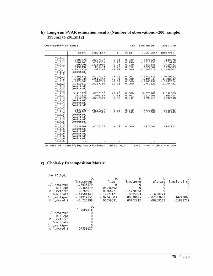
75 | P a g e
b) Long-run SVAR estimation results (Number of observations =200, sample:
1995m1 to 2011m12)
c) Cholesky Decomposition Matrix
LR test of identifying restrictions: chi2( 6)= 3943 Prob > chi2 = 0.000 /c_6_6 1 . . . . . /c_5_6 (omitted) /c_4_6 (omitted) /c_3_6 (omitted) /c_2_6 (omitted) /c_1_6 (omitted) /c_6_5 .2956908 .0707107 4.18 0.000 .1571004 .4342812 /c_5_5 1 . . . . . /c_4_5 (omitted) /c_3_5 (omitted) /c_2_5 (omitted) /c_1_5 (omitted) /c_6_4 .0047021 .0737371 0.06 0.949 -.13982 .1492243 /c_5_4 -.0133597 .0707107 -0.19 0.850 -.1519501 .1252307 /c_4_4 1 . . . . . /c_3_4 (omitted) /c_2_4 (omitted) /c_1_4 (omitted) /c_6_3 -.0347778 .0737379 -0.47 0.637 -.1793014 .1097458 /c_5_3 .0271123 .070717 0.38 0.701 -.1114905 .165715 /c_4_3 3.413779 .0707107 48.28 0.000 3.275189 3.552369 /c_3_3 1 . . . . . /c_2_3 (omitted) /c_1_3 (omitted) /c_6_2 1.119817 .0737789 15.18 0.000 .9752126 1.264421 /c_5_2 -.6774061 .070743 -9.58 0.000 -.8160598 -.5387524 /c_4_2 -4.001635 .2515342 -15.91 0.000 -4.494633 -3.508637 /c_3_2 -.2165835 .0707107 -3.06 0.002 -.3551739 -.0779931 /c_2_2 1 . . . . . /c_1_2 (omitted) /c_6_1 -.9715529 .1082279 -8.98 0.000 -1.183676 -.7594302 /c_5_1 -.0198192 .085434 -0.23 0.817 -.1872667 .1476283 /c_4_1 .0290098 .3785959 0.08 0.939 -.7130246 .7710441 /c_3_1 .0202201 .0723501 0.28 0.780 -.1215835 .1620238 /c_2_1 .0009876 .0707107 0.01 0.989 -.1376028 .139578 /c_1_1 1 . . . . . Coef. Std. Err. z P>|z| [95% Conf. Interval]
Overidentified model Log likelihood = -2085.759Sample: 1960m6 - 1977m1 No. of obs = 200
D.l_dcredit .07358627D.l_multip~r 0 D.wlbrate 0 D.l_metprxn 0 D.l_cpi 0D.l_reserves 0 l_dcredit D.
D.l_dcredit -1.730398 .06059691 .00472212 .00969559 .01883717D.l_multip~r -.01917851 -.02743303 .00830695 -.02833687 .14247863 D.wlbrate -.41581143 -.12571121 .0395993 2.3758771 0 D.l_metprxn .00786911 .00768771 .15770978 0 0 D.l_cpi .00388879 .05046662 0 0 0D.l_reserves 1.7938579 0 0 0 0 l_reserves l_cpi l_metprxn wlbrate l_multiplier D. D. D. D. D.choll2[6,6]

76 | P a g e
d) SVAR Impulse Response Functions Graphs
-10
0
10
-10
0
10
-10
0
10
-10
0
10
-10
0
10
-10
0
10
0 5 10 15 0 5 10 15 0 5 10 15 0 5 10 15 0 5 10 15 0 5 10 15
test2, D.l_cpi, D.l_cpi test2, D.l_cpi, D.l_dcredit test2, D.l_cpi, D.l_metprxn test2, D.l_cpi, D.l_multiplier test2, D.l_cpi, D.l_reserves test2, D.l_cpi, D.wlbrate
test2, D.l_dcredit, D.l_cpi test2, D.l_dcredit, D.l_dcredit test2, D.l_dcredit, D.l_metprxn test2, D.l_dcredit, D.l_multiplier test2, D.l_dcredit, D.l_reserves test2, D.l_dcredit, D.wlbrate
test2, D.l_metprxn, D.l_cpi test2, D.l_metprxn, D.l_dcredit test2, D.l_metprxn, D.l_metprxn test2, D.l_metprxn, D.l_multiplier test2, D.l_metprxn, D.l_reserves test2, D.l_metprxn, D.wlbrate
test2, D.l_multiplier, D.l_cpi test2, D.l_multiplier, D.l_dcredit test2, D.l_multiplier, D.l_metprxn test2, D.l_multiplier, D.l_multiplier test2, D.l_multiplier, D.l_reserves test2, D.l_multiplier, D.wlbrate
test2, D.l_reserves, D.l_cpi test2, D.l_reserves, D.l_dcredit test2, D.l_reserves, D.l_metprxn test2, D.l_reserves, D.l_multiplier test2, D.l_reserves, D.l_reserves test2, D.l_reserves, D.wlbrate
test2, D.wlbrate, D.l_cpi test2, D.wlbrate, D.l_dcredit test2, D.wlbrate, D.l_metprxn test2, D.wlbrate, D.l_multiplier test2, D.wlbrate, D.l_reserves test2, D.wlbrate, D.wlbrate
95% CI impulse response function (irf)
step
Graphs by irfname, impulse variable, and response variable