WP/06/80

A Practical Model-Based Approach to Monetary Policy Analysis—Overview

Andrew Berg, Philippe Karam, and Douglas Laxton

© 2006 International Monetary Fund WP/06/80

IMF Working Paper

Policy Development and Review Department, Research Department, and IMF Institute

A Practical Model-Based Approach to Monetary Policy Analysis—Overview

Prepared by Andrew Berg, Philippe Karam, and Douglas Laxton1

Authorized for distribution by Andrew Berg, Gian Maria Milesi-Ferretti, and Ralph Chami

March 2006

Abstract

This Working Paper should not be reported as representing the views of the IMF. The views expressed in this Working Paper are those of the author(s) and do not necessarily represent those of the IMF or IMF policy. Working Papers describe research in progress by the author(s) and are published to elicit comments and to further debate.

This paper motivates and describes an approach to forecasting and monetary policy analysis based on the use of a simple structural macroeconomic model, along the lines of those in use in a number of central banks. It contrasts this approach with financial programming and its emphasis on monetary aggregates, as well as with more econometrically driven analyses. It presents illustrative results from an application to Canada. A companion paper provides a more detailed how-to guide and introduces a set of tools designed to facilitate this approach. JEL Classification Numbers: E52, E47, C51 Keywords: Monetary policy, forecasting and simulation, model construction, and estimation Author(s) E-Mail Address: aberg@imf.org, pkaram@imf.org, dlaxton@imf.org

1 The framework outlined here is being used by several IMF desk economists who meet regularly to share experiences, solve problems, and present results—Ricardo Adrogue, Zsofia Arvai, Roberto Benelli, Natan Epstein, Thomas Harjes, Ben Hunt, Jorge Canales Kriljenko, Irineu Evangelista de Carvalho Filho, Roberto Garcia-Saltos, Eva Jenkner, Meral Karasulu, Daniel Leigh, Rodolfo Luzio, Vincent Moissinac, Susanna Mursula, Papa N’Diaye, Anton Nakov, Hang Thi Thu Nguyen, Luca Ricci, Pau Rabanal, and Ivan Tchakarov. We would like to thank Alin Mirestean and Kexue Liu for providing support to new members of the team. We thank Jamie Armour, André Binette, and Patrick Perrier (Bank of Canada), and David Reifschneider (Federal Reserve Board) who generously shared data and simulation results. We also thank Shekhar Aiyar, Andrew Feltenstein, Charles Freedman, Peter Isard, Gian Maria Milesi-Ferretti, G. Russell Kincaid, Tohkir Mirzoev, and Carlo Sdralevich for their helpful comments on an earlier draft, Pille Snydstrup for editorial assistance, and Asmahan Bedri and Lei Lei Myaing for their work on the graphs and tables.

- 2 -

Contents Page I. Introduction ........................................................................................................................... 3 II. Monetary Policy Analysis at the Fund ................................................................................. 5

A. Financial Programming as a Tool for Monetary Policy Analysis.................................... 5 B. Econometric Models ........................................................................................................ 8

III. Macroeconomic Modeling .................................................................................................. 9 A. The Role of Macroeconomic Models............................................................................... 9 B. The Model ...................................................................................................................... 11

IV. Building the Model ........................................................................................................... 17 V. Forecasting and Policy Analysis ........................................................................................ 20 VI. An Example. ..................................................................................................................... 22

A. Overview........................................................................................................................ 22 B. Building the model ......................................................................................................... 23 C. Using the Model for Forecasting and Policy Analysis at the IMF................................. 25

VII. Caveats and Future Work ................................................................................................ 27 VIII. Conclusions.................................................................................................................... 29 References............................................................................................................................... 39 Tables 1. Baseline Forecast with Desk Judgment – WEO Scenario...................................................36 2. Canada: Canadian Interest Rate Shock – One Quarter Increase of 100 b.p. .....................37 3. United States: U.S. Interest Rate Shock – One Quarter Increase of 100 b.p. ....................38 Figures 1. Output Growth, Inflation, Interest Rates, and Exchange Rates: Canada and the United

States………………………………………………………………………………………31 2. Model Variables for Canada................................................................................................32 3. Model Variables for the United States.................................................................................33 4. Dynamic Responses of Output, Inflation, and Short-Term Interest Rates: Comparing

SMPMOD and QPM............................................................................................................34 5. Dynamic Responses of Output, Inflation, and Short-Term Interest Rates: Comparing

SMPMOD and FRBUS........................................................................................................35

- 3 -

"All models are wrong! Some are useful" –George Box2

I. INTRODUCTION

Twenty years ago, standard academic treatments of monetary policy analysis did not satisfy policymakers' needs. The focus was on building microeconomic foundations for various features of the monetary transmission mechanism, for example capturing the implications of a cash-in-advance constraint for money demand. Modeling efforts centered on real business cycle dynamic general equilibrium frameworks in which markets continuously cleared and there was little scope for monetary policy. Policymakers had to rely on ad hoc models such as IS/LM and Mundell-Fleming that lacked adequate treatment of expectations and stock-flow relationships.3 In recent years, economists have learned how to build simple, coherent, and plausible models of the monetary transmission mechanism. In the New Keynesian synthesis, there has been a convergence between the useful empirically motivated IS/LM models developed in several policymaking institutions and dynamic stochastic general equilibrium approaches that take expectations seriously and are built on solid microeconomic foundations. The simple workhorse model now consists of an aggregate demand (or IS) curve, a price-setting (or Phillips) curve, and a policy reaction function relating the policy interest rate to variables like output and inflation. These sorts of models embody the basic principle that the fundamental role for monetary policy is to provide an anchor for inflation and inflation expectations. They are consistent with a view of the world familiar to policymakers, a world in which: because of nominal and real rigidities, aggregate demand determines output in the short run; expectations matter for inflation and output; and monetary policy is expressed in terms of a rule for setting the nominal interest rate.4 Small (or for that matter large) structural models themselves do not produce accurate forecasts. Any good baseline forecast is based mostly on judgment.5 Rather, these models are useful because they assemble various understandings about how the economy works into a coherent whole, so that joint implications can be assessed. Forecasts can be explicit about policy reactions, the source of shocks, and risks resulting from different assumptions about the functioning of the economy. For example, is the inflation target expected to be met in the 2George E.P. Box and Norman R. Draper, “Empirical Model-Building and Response Surfaces” (Wiley 1987) pp. 424. 3In a popular graduate textbook by Blanchard and Fischer (1989), the presentation of these types of models was relegated to the last chapter entitled "Some Useful Models." 4We have obviously not done justice to this story here. Recent surveys include Clarida, Gertler and Gali (1999), Lane (2001), and Woodford (2003a).

5 For a description about the role of judgment in the macro forecasts that are used in central banks see Sims (2002) and Svennson and Tetlow (2005). Romer and Romer (2000) and Sims (2002) show that the judgemental forecasts made at the Fed are better than pure model-based forecasts.

- 4 -

future given the current stance of monetary policy and the output gap? What if exchange rate pass-through is lower than in the past? They can also shed light on the implications of following different sorts of policy rules. If the authorities "lean against the wind" with respect to exchange rate movements, what happens to output and inflation volatility? Moreover, above all these things, the use of macro models can provide a systematic methodology for assessing the policy implications of uncertainty by providing a framework for analyzing and characterizing the risks around any conditional baseline macroeconomic projection path. Macroeconomic models such as those we discuss here have become important tools for many central banks.6 This reflects the models’ ability to help policymakers structure their thinking, discussions, and forecasting exercises. For inflation targeting central banks, there is an extra bonus. A key feature of inflation targeting is the communication with the public of the rationale for the monetary policy stance, so as to coordinate expectations around the desired outcome. A small, coherent, and sensible economic model is a useful vehicle for this sort of communication.7 This paper is motivated by the impression that the approach presented here would be a useful addition to the standard toolkit of. IMF economists, who produce a large number of modern analyses of various aspects of monetary policy, including those using methods more sophisticated than those we discuss in this paper.8 This has not, however, systematically influenced the standard analytic tools used by most country teams in their nuts-and-bolts operational work. In several instances in recent years, staff teams have in their country work applied analyses broadly of the sort we are advocating here. However, in the absence of easily available tools and a community of like-minded analysts, these initiatives have remained isolated. Our goal is to try to generalize and strengthen these efforts. The typical country application of this approach would be to a country with a floating exchange rate regime and a formal or implicit inflation targeting monetary framework. The framework can be applied to countries in which the float is managed, either in the sense that monetary policy reacts to the exchange rate or that there is substantial foreign exchange intervention.

6The degree of complexity and sophistication of macroeconomic models varies considerably across central banks. Models broadly along the lines of that presented here have often formed the basis of successful modeling efforts. Several institutions are building a new generation of core workhorse models with stronger choice-theoretic foundations. However, it is wise to start with simpler models to begin with and then develop more sophisticated systems over time—see Laxton and Scott (2000).

7Laxton and Scott (2000) and Canales-Kriljenko and others (2005) discuss the role of models as well as the full range of related issues in operationalizing an inflation targeting framework.

8 See for example Leigh (2005), Parrado (2004), and Eggertson and Woodford (2003).

- 5 -

A key feature of this approach is that the economic structure of the model is more important than purely fitting the data. Indeed, we suggest following the practice of most central banks and taking an eclectic approach to determining the parameters of the model. A purely econometric approach, in which a general set of equations is fit to the data, does not generally result in a useful model. The economy is characterized by a high degree of simultaneity and forward-looking behavior, while data series are generally short and subject to structural change, for example in the monetary policy regime. In this context, it is not possible to reliably estimate parameters and infer cause and effect. More fundamentally, purely empirically based models do not permit the analysis of changes in policy rules or changes in the assumptions about how the economy works. For purposes of policy analysis, the model must first of all be identified, in that each of the equations has a clear economic interpretation. Thus, rather than estimate a reduced-form empirically based model whose structural interpretation is doubtful, we suggest using a broader collection of information to help parameterize a structural macroeconomic model. The goal of this paper is to motivate and describe a macro-model based approach to forecasting and monetary policy analysis. The next section reviews the current practice of monetary policy analysis at the Fund and discusses various alternative approaches. Section III introduces and discusses a simple benchmark New Keynesian model. Section IV discusses how to match the model with reality. Section V describes how to conduct a forecasting and monetary policy analysis with the model. Section VI puts the model through its paces, parameterizing it for Canada and carrying out a forecasting and risk assessment exercise. Section VII provides caveats and suggestions for future work. Section VIII concludes. A companion paper (Berg, Karam, and Laxton, 2006) enters into more detail and introduces a set of tools designed to facilitate the implementation of this approach.9 We hope that many economists engaged in applied policy analysis at the IMF will adopt and eventually develop and enrich these tools, moving on to richer models as necessary. We also expect that insights these economists gain will in turn be useful to the broader academic community.

II. MONETARY POLICY ANALYSIS AT THE IMF

A. Financial Programming as a Tool for Monetary Policy Analysis

The central analytic framework for IMF program design and policy analysis remains financial programming, whose central task is the design of a consistent set of policies intended to move an economy toward internal and external balance. Macroeconomic aggregates are traditionally derived from an interconnected set of macroeconomic accounts: the national income and product accounts, the balance of payments, government finance 9The two papers overlap substantially. This paper targets mainly newcomers to modern structural macroeconomic modeling and potential consumers. The “how-to-guide” contains more nuts-and bolts details for modelers. It thus abbreviates the material contained in sections II and IIIA of this paper and expands on the rest.

- 6 -

statistics and the monetary accounts. Financial programming combines these accounts and formulates internally consistent macroeconomic forecasts of the economy under consideration. This framework has value as a consistency check and when it is applied in combination with an appealing set of behavioral relations and assumptions.10 As a guide to the analysis and conduct of monetary policy, however, the framework has limited applicability. The standard analytic framework for the analysis of monetary policy has concentrated on monetary aggregates.11 At the core is a key relation for monetary policy analysis known as the quantity equation: pymv = where m is an appropriate monetary aggregate (such as base money), p is the relevant price level, y is real output, and v is (by definition) the velocity of money. The economics comes from the thought that velocity is a function of interest rates and other factors. In practice, the analyst provides a set of forecasts for p and y. An assumption made about the path of v then implies an appropriate path for m. The balance sheet identity of the central bank equates m to the level of international reserves, R, plus net domestic assets, NDA. Typically, a Fund program would embody a floor for the path of R and a ceiling for the path of NDA consistent with the appropriate path for m. In the broader academic and policy making community, the move away from a focus on monetary aggregates has been dramatic and is now nearly complete. Monetary policy without money is the benchmark in standard undergraduate and graduate texts, reflecting analytic developments and, most importantly, central bank practice around the world. In the words of Benjamin Friedman (2003), "One of the most significant changes in monetary economics in recent years has been the virtual disappearance of what was once a dominant focus on money . . . as part of the analytical framework that economists use to think about issues of monetary policy."12 The financial programming approach to monetary policy analysis may remain relevant when direct central-bank financing of the fiscal deficit is a central policy concern, particularly for a fixed exchange rate regime. In this context, financial programming usefully emphasizes that more credit to government, and thus NDA, implies fewer reserves, given a path for money balances. In middle-income and developed countries, however, monetary policy is more frequently being formulated in a context of a managed floating exchange rate and a formal or informal 10IMF (2004a) provides a recent official description and assessment of financial programming, emphasizing its usefulness as an organizing framework and the need to supplement it with other tools in particular circumstances.

11See IMF (2004b).

12Leeper and Roush (2003) also make this point and cite as examples Romer (2000), Stiglitz and Walsh (2002), and Woodford (2003a). Clarida, Gali and Gertler (1999) estimate monetary policy reaction functions for several countries and argue that even avowed money targeters such as the Bundesbank did not in fact practice targeting monetary aggregates. Stone and Bhundia (2004) survey large and more developed countries (75-85 countries) and point out that money targets were used by only five countries in 1990, and by 2000 this regime became extinct.

- 7 -

inflation-targeting regime, and largely independently of the fiscal authorities. In this situation, financial programming provides little guidance for the conduct of monetary policy. First, money demand rarely serves as an anchor for the conduct of monetary policy. As has been widely recognized, money demand is often too unstable to be relied upon as a framework for setting the stance of monetary policy. More importantly, even a stable money demand curve typically implies large idiosyncratic movements in money demand. It is rarely possible to isolate the shocks to money demand from the policy shocks that are of interest.13 Most fundamentally, this framework does not provide a useful framework for talking about monetary policy. Central questions involve issues such as whether the policy interest rate is set correctly, how the authorities should react to exchange rate movements, how the forecast depends on various economic assumptions, and so on. The financial-programming framework buries this entire discussion in the determination of velocity and its relationship to interest rates. Discussions frequently revolve around explanations, largely ex post rationalizations, for observed movements of money aggregates. Where central banks have ceased to employ a financial programming framework, the value of the Fund relying on this procedure to frame discussions is particularly low. Staff cannot easily engage with the counterparts on a technical level, nor do interactions with Fund staff serve to sharpen the technical discussions within the central bank—a lost opportunity.14 The staff is aware of these problems. Moreover, as Mussa and Savastano (2000) emphasize, financial programming is an accounting framework only and does not in itself force Fund economists into particular policy conclusions. The implications remain serious, nonetheless. The excessive reliance on financial programming implies that staff may not have sufficient analytic support in thinking about monetary policy issues. And financial programming, as the only readily available tool, often receives too much weight. This may be a reflection of the well-documented phenomenon known in the behavioral finance literature as the "anchoring heuristic," in which decision processes are often dominated by available pieces of information even if they are obviously of no relevance.15 13IMF (2004a) provides an in-depth discussion of analytic frameworks and program design in Fund-supported programs. It notes the usefulness of financial programming as an organizing framework as well as the need to supplement it with other tools in particular circumstances. IMF (2004b) analyzes the experience with monetary aggregates in Fund-supported programs. It concludes that the high correlation between monetary aggregates and inflation reaffirms the importance of nominal anchors for controlling inflation. Berg and others (2003) discuss monetary policy in post-crisis situations and argue that, even in those cases, there is little practical role for monetary aggregates in the assessment of monetary policy in practice.

14The question of the role of financial programming in Fund conditionality is a related but distinct question that is outside the scope of this paper. In IMF programs, the value of traditional monetary aggregate conditionality resides partly in its “safety” features. In this case, the monetary aggregate targets are not meant to structure thinking or policy with respect to “everyday” monetary policy choices but rather to identify gross breaches of the policy. Blejer and others (2001) discuss the difficulties involved in applying standard Fund quantitative performance criteria for monetary policy to countries that follow an inflation-targeting regime.

15 Bofinger and Schmidt (2004) rely on the anchoring heuristic to explain the otherwise puzzling tendency of professional foreign exchange forecasters to perform substantially worse than a naïve random walk and, in particular, to pay too much attention to actual changes in the exchange rate.

- 8 -

B. Econometric Models

Fund staff has in recent years sought more useful analytic frameworks for thinking about monetary policy. One approach has been to estimate empirically-motivated inflation equations, often in the context of a VAR with equilibrium correction.16 While sometimes useful, this approach has several major drawbacks. First, there are rarely enough data for reliable inference. In most countries, the current monetary policy regime has been in place for only a few years. In an economy in which expectations play a key role and everything tends to depend on everything else, inference in such samples is unreliable. A more fundamental problem with econometric approaches for our purposes is that the nonstructural data-based approach does not lend itself to answering the questions of interest to policymakers. For example, where countries are seeking to better anchor inflation expectations in order to reduce inflation persistence and real volatility, it makes little sense to employ a statistical methodology that hard wires policy parameters in reduced-form equations and provides no direct role for policy to change them. An emphasis on data fitting can lead, in practice, to models that lack critical features such as forward-looking inflation expectations, on the grounds that such features are much harder to implement empirically. The absence of such features makes estimated models misspecified and, of course, also more vulnerable to the Lucas critique, in that changes in the monetary policy reaction function, for example, lose a channel through which they influence other equations. Similarly, classical hypothesis testing asks the wrong sorts of questions. For example, an econometric estimation of the equation for output determination might start by testing the null hypotheses that the interest rate does not affect the output gap or the exchange rate. In small samples, we might well not be able to reject the nulls. In thinking about the monetary policy transmission mechanism, though, these are uninteresting hypotheses. In practice, this methodology has sometimes produced models with very weak monetary transmission mechanisms, where extremely large changes in interest rates would be necessary to anchor inflation to the target in response to shocks that continuously disturb the economy. The structural vector autoregression (SVAR) approach attempts to make explicit identifying assumptions in order to be able to give the estimates structural interpretations. These identifying assumptions usually take the form of restrictions in contemporaneous reaction of one variable to shocks emanating from another variable. Unfortunately, in a simultaneous economy in which expectations are important, it is extremely difficult to credibly identify the key equations, in other words to assert with any confidence that one equation is really an "inflation" equation and the shocks are shocks to the price level, while another equation is a monetary policy equation. The identification problem is particularly difficult when the model includes two asset prices, for example the interest rate and the exchange rate. In this situation, each is likely to depend on the other at any frequencies, rendering dubious any identification depending on the typical contemporaneous exclusion restrictions. 16Garratt and others (2003) estimate a small quarterly model for the United Kingdom.

- 9 -

A related approach estimates a vector equilibrium correction model and avoids making explicit assumptions to identify the equations. An equation normalized so that inflation is on the left-hand side is considered to represent the underlying economic process for inflation, based on the plausibility of the estimated signs and parameter stability in the face of shocks to other equations (“super-exogeneity”). This approach may serve in forecasting but, even more than the SVAR strategy, cannot be relied on to produce reliable structural models of the economy.17 The most fundamental problem with econometrically-driven approaches is that policy-makers need first of all a model that is economically meaningful and transparent, and that allows them to study the implications of various economic assumptions and policy interventions. In other words, they need a structural macro model. In the next section, we discuss alternatives. We do not suggest eschewing econometrics entirely, and in Section IV we return to the uses of econometrics in the context of the question of how to parameterize simple structural models.

III. MACROECONOMIC MODELING

A. The Role of Macroeconomic Models Macroeconomic models for monetary policy analysis are designed to describe the interactions of key macroeconomic variables over the medium term. The main purpose is not to produce a forecast understood as best guess of the values of the main variables. In practice, models do not produce the forecast, economists do. What models can do is provide a coherency check on the judgment that produces the main forecast. They allow the systematic analysis of risks to the forecast, including sensitivity to various assumptions, shocks, and policy responses. Most importantly, they provide a framework that can help to ask the right questions. We propose here that analysis center around a small core model with only four key behavioral equations. This model attempts to allow for consistent projections for real GDP, inflation, the real interest rate, and the real exchange rate, all in terms of deviations from equilibrium levels. Its advantage is that it can be relatively transparent and simple and still allow consideration of the key features of the economy for monetary policy analysis.

17 See Faust and Whiteman (1997).

- 10 -

Such a model is silent on a number of critical issues. It abstracts from issues related to aggregate supply and fiscal solvency and does not explore the determinants of the current account, the equilibrium levels of real GDP, the real exchange rate or the real interest rate. These considerations are of course essential to policy analysis and forecasting. The framework described below allows judgment about them to be incorporated into the model’s forecasts and the implications of different assumptions explored. But the model itself provides little direct help in articulating their determinants. Because the model abstracts from so many issues, there may be a tendency to add various features to the model. Models such as those we propose below are, in somewhat more complicated form, at the heart of both central bank practice and enormous current research efforts worldwide. Thus, there is great scope to develop the model further. It is important, though, that additions not detract from the clarity of the model. Where the skills and resources are available, the model may be extended to include full microeconomic foundations, stock-flow dynamics, non-traded sectors, and other features that allow explicit treatment of a number of additional issues.18 The model should not be allowed to become a “black box” however. One intermediate approach may be to build an auxiliary model for, say, fiscal policy, which considers the expenditure component of government spending, the implications for households’ intertemporal savings decisions, and ways of thinking about Ricardian Equivalence, the debt stock, and so on. The overall implications of fiscal policy for aggregate demand could then be integrated into the core model.19 The model presented here blends the New Keynesian emphasis on nominal and real rigidities and a role of aggregate demand in output determination, with the real business cycle tradition methods of dynamic stochastic general equilibrium (DSGE) modeling with rational expectations. The model is structural because each of its equations has an economic interpretation. Causality and identification are not in question. Policy interventions have counterparts in changes in parameters or shocks, and their influence can be analyzed by studying the resulting changes in the model’s outcomes. It is general equilibrium because the main variables of interest are endogenous and depend on each other. It is stochastic in that random shocks affect each endogenous variable and it is possible to use the model to derive measures of uncertainty in the underlying baseline forecasts. It incorporates rational expectations because expectations depend on the model's own forecasts, so there is no way to consistently fool economic agents.20 18The IMF’s Global Economy Model (GEM), described in Laxton and Pesenti (2003), for example, represents such a model. The set of tools that we rely upon for our simple model, described in an Appendix in the companion paper, are similar to those required to work with GEM.

19Coats, Laxton and Rose (2003) describe how such an approach is practiced in the Czech Republic, based on a core model along the lines described in this paper. The IMF has developed a multi-country, new-open-economy macro model to study the medium-term and long-term implications of fiscal policies. See Botman and others (2006).

20We say “consistently” because it may be appropriate to extend the model to incorporate an element of adaptive expectations.

- 11 -

Such models are often derived explicitly from microeconomic foundations in the literature.21 The core elements include consumers who maximize expected utility and firms that are subject to monopolistic competition who adjust prices only periodically. Such micro-foundations are ultimately critical and should play a central role in determining the model's specification insofar as the model itself must be coherent and embody the economic ideas the modeler wishes to emphasize. However, we do not derive our baseline model below from microeconomic foundations. We allow for adaptive as well as rational expectations and substantial inertia in the equations. We could appeal to theory to justify these features, but we do not believe that, in practice, appealing to specific micro foundations serves to tie down magnitudes. We believe that this pragmatic approach to modeling represents the current state of the art in many policymaking institutions, where modelers “engage but don’t marry theory.”22

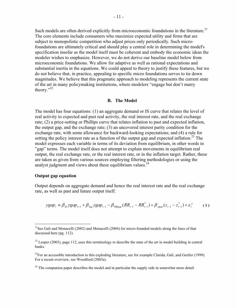
B. The Model The model has four equations: (1) an aggregate demand or IS curve that relates the level of real activity to expected and past real activity, the real interest rate, and the real exchange rate; (2) a price-setting or Phillips curve that relates inflation to past and expected inflation, the output gap, and the exchange rate; (3) an uncovered interest parity condition for the exchange rate, with some allowance for backward-looking expectations; and (4) a rule for setting the policy interest rate as a function of the output gap and expected inflation.23 The model expresses each variable in terms of its deviation from equilibrium, in other words in ”gap” terms. The model itself does not attempt to explain movements in equilibrium real output, the real exchange rate, or the real interest rate, or in the inflation target. Rather, these are taken as given from various sources employing filtering methodologies or using the analyst judgment and views about these equilibrium values.24 Output gap equation

Output depends on aggregate demand and hence the real interest rate and the real exchange rate, as well as past and future output itself.

ytttzgapttRRgaptlagtldt zzRRRRygapygapygap εββββ +−+−−+≡ −−−−−+ )()( *

11*

1111 ( 1 )

21See Gali and Monacelli (2002) and Monacelli (2004) for micro-founded models along the lines of that discussed here (pg. 112).

22 Leeper (2003), page 112, uses this terminology to describe the state of the art in model building in central banks.

23For an accessible introduction to this exploding literature, see for example Clarida, Gali, and Gertler (1999). For a recent overview, see Woodford (2003a).

24 The companion paper describes the model and in particular the supply side in somewhat more detail.

- 12 -

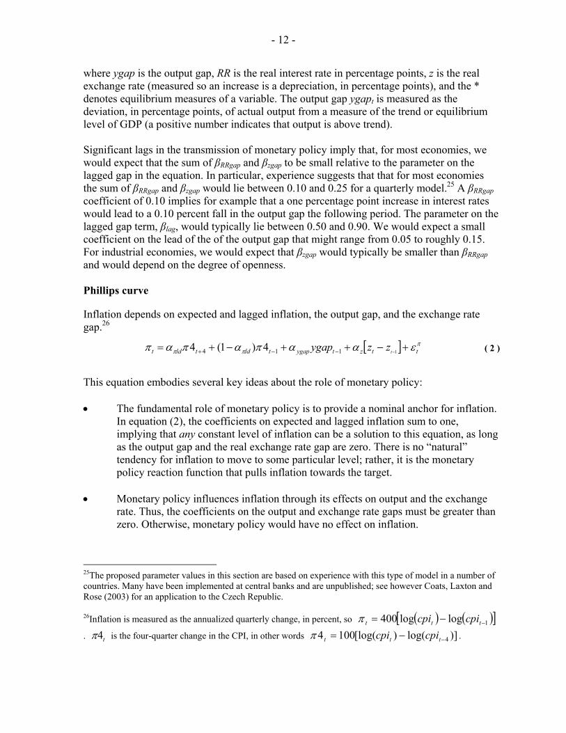
where ygap is the output gap, RR is the real interest rate in percentage points, z is the real exchange rate (measured so an increase is a depreciation, in percentage points), and the * denotes equilibrium measures of a variable. The output gap ygapt is measured as the deviation, in percentage points, of actual output from a measure of the trend or equilibrium level of GDP (a positive number indicates that output is above trend). Significant lags in the transmission of monetary policy imply that, for most economies, we would expect that the sum of βRRgap and βzgap to be small relative to the parameter on the lagged gap in the equation. In particular, experience suggests that that for most economies the sum of βRRgap and βzgap would lie between 0.10 and 0.25 for a quarterly model.25 A βRRgap coefficient of 0.10 implies for example that a one percentage point increase in interest rates would lead to a 0.10 percent fall in the output gap the following period. The parameter on the lagged gap term, βlag, would typically lie between 0.50 and 0.90. We would expect a small coefficient on the lead of the of the output gap that might range from 0.05 to roughly 0.15. For industrial economies, we would expect that βzgap would typically be smaller than βRRgap and would depend on the degree of openness. Phillips curve

Inflation depends on expected and lagged inflation, the output gap, and the exchange rate gap.26

[ ] πππ εααπαπαπ ttztygaptldtldt tzzygap +−++−+= −−−+ 1114 4)1(4 ( 2 )

This equation embodies several key ideas about the role of monetary policy: • The fundamental role of monetary policy is to provide a nominal anchor for inflation.

In equation (2), the coefficients on expected and lagged inflation sum to one, implying that any constant level of inflation can be a solution to this equation, as long as the output gap and the real exchange rate gap are zero. There is no “natural” tendency for inflation to move to some particular level; rather, it is the monetary policy reaction function that pulls inflation towards the target.

• Monetary policy influences inflation through its effects on output and the exchange

rate. Thus, the coefficients on the output and exchange rate gaps must be greater than zero. Otherwise, monetary policy would have no effect on inflation.

25The proposed parameter values in this section are based on experience with this type of model in a number of countries. Many have been implemented at central banks and are unpublished; see however Coats, Laxton and Rose (2003) for an application to the Czech Republic.

26Inflation is measured as the annualized quarterly change, in percent, so ( ) ( )[ ]1loglog400 −−= ttt cpicpiπ

. t4π is the four-quarter change in the CPI, in other words )]log()[log(1004 4−−= ttt cpicpiπ .

- 13 -

• The central bank cannot consistently fool people. To ensure this, the coefficient on expected inflation must be positive. If instead απld is zero, then the central bank could keep output permanently above equilibrium by constantly “surprising” agents with higher-than-expected inflation.

A standard derivation from microeconomic foundations assuming optimizing firms with rational expectations implies that expectations depend only on future inflation, so απld = 1. A value less than 1 can be rationalized as resulting from the idea that there is a component of backward-looking expectations based for example on learning, imperfect credibility of the central bank, or indexation. The behavior of the economy depends critically on the value of απld. If inflation expectations are entirely forward looking (απld is equal to 1), then inflation is equal to the sum of all future output and exchange rate gaps. A small but persistent increase in interest rates will have a large and immediate effect on current inflation. In this “speedboat” economy, small recalibrations of the monetary-policy wheel, if perceived to be persistent, will cause large jumps in inflation through forward-looking inflation expectations. If expectations are largely backward-looking, on the other hand (απld is close to 0), then current inflation is a function of lagged values of the gaps, and only an accumulation of many periods of interest rate adjustments can move current inflation toward some desired path. In this “aircraft carrier” economy, the wheel must be turned well in advance of the date at which inflation will begin to change substantially. Where price-setting is flexible and the monetary authorities are fully credible, high values of απld might be reasonable, but for most countries values of απld significantly below 0.50 seem to produce results that are usually considered to be more consistent with data. The value of αz determines the effects of exchange rate changes on inflation. αz would typically be larger in economies that are very open. Higher exchange rate pass-through is generally also observed in countries where monetary policy credibility is low and where the value-added of the distribution sector is low. There is significant evidence of pricing-to- market behavior in many economies, suggesting that αz would be considerably smaller than the import weight in the CPI basket.27 Exchange rate

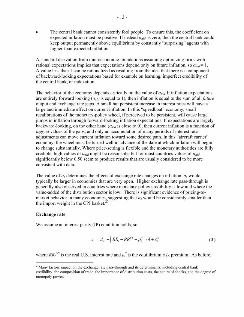
We assume an interest parity (IP) condition holds, so:

*1 / 4e US z

t t t t t tz z RR RR ρ ε+ ⎡ ⎤= − − − +⎣ ⎦ ( 3 )

where RRt

US is the real U.S. interest rate and ρt* is the equilibrium risk premium. As before,

27Many factors impact on the exchange rate pass-through and its determinants, including central bank credibility, the composition of trade, the importance of distribution costs, the nature of shocks, and the degree of monopoly power.

- 14 -

RRt is the policy real interest rate and zt is the real exchange rate. The interest rate term is divided by 4 because the interest rates and the risk premium are measured at annual rates, where zt is quarterly.28 We assume a coefficient of one on the interest rate differential, as implied by the IP condition. This result has been frequently challenged empirically. In defense of this assumption, the simultaneity involving interest rates and exchange rates makes any effort to estimate this coefficient particularly difficult. The estimated coefficient on the interest rate differential will be biased downward to the extent that the monetary authorities “lean against the wind” of exchange rate movements.29

We allow but do not impose (model-consistent) rational expectations for the exchange rate:

( ) 111 1 −++ −+= tztzet zzz δδ ( 4 )

When δz = 1, we recover Dornbusch (1976) overshooting dynamics. In practice, overshooting often seems to take place in slower motion, and a value of δz somewhat less than 1 may provide more realistic dynamics. Unfortunately, there is little consensus across countries or observers on a reasonable value for δz .30 Monetary policy rule

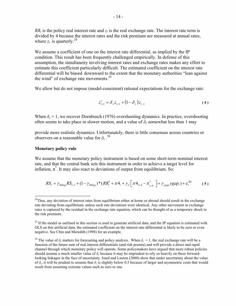
We assume that the monetary policy instrument is based on some short-term nominal interest rate, and that the central bank sets this instrument in order to achieve a target level for inflation, π*. It may also react to deviations of output from equilibrium. So:

* *1 4 4

(1 )*( 4 4 ) RSt RSlag t RSlag t t t ygap t tt

RS RS RR ygapπγ γ π γ π π γ ε− + +⎡ ⎤= + − + + − + +⎣ ⎦ ( 5 )

28Thus, any deviation of interest rates from equilibrium either at home or abroad should result in the exchange rate deviating from equilibrium, unless such rate deviations were identical. Any other movement in exchange rates is captured by the residual in the exchange rate equation, which can be thought of as a temporary shock to the risk premium.

29 If the model as outlined in this section is used to generate artificial data, and the IP equation is estimated with OLS on this artificial data, the estimated coefficient on the interest rate differential is likely to be zero or even negative. See Chin and Meredith (1998) for an example.

30 The value of δz matters for forecasting and policy analysis. When δz = 1, the real exchange rate will be a function of the future sum of real interest differentials (and risk premia) and will provide a direct and rapid channel through which monetary policy will operate. Some policymakers have argued that more robust policies should assume a much smaller value of δz because it may be imprudent to rely so heavily on these forward-looking linkages in the face of uncertainty. Isard and Laxton (2000) show that under uncertainty about the value of δz, it will be prudent to assume that δz is slightly below 0.5 because of larger and asymmetric costs that would result from assuming extreme values such as zero or one.

- 15 -

The structure and parameters of this equation have a variety of implications.31 An important conclusion from assessments of monetary policy in the 1970s, and one embedded in the structure of this model, is that a stable inflation rate requires a positive πγ .32 Beyond this, our framework does not allow explicit discussion of optimality, in the absence of microeconomic foundations.33 But it may be useful to note that how strongly the authorities should react depends on the other features of the economy. If the economy is very forward-looking, for example, as implied by the “speedboat” version of the Phillips curve, then moderate but persistent reactions to expected inflation should be enough to keep inflation close to target. If, on the other hand, the Phillips curve is of the “aircraft carrier” type, then a forward-looking approach to monetary policy may require a more aggressive reaction. Following Woodford (2003b), we allow for the possibility that the central bank smoothes interest rates, adjusting them fairly slowly to the desired value based on deviations of inflation and output from equilibrium. In typical empirically-based reaction functions the value for RSlagγ falls between 0.50 and 1.0. Arguments other than inflation and output may belong in the reaction function.34 A variety of papers have explored in particular the question of whether the exchange rate belongs in the reaction function. In general, adding the exchange rate typically makes little difference when uncovered interest parity holds, because in this case the exchange rate is purely a function of expected future interest rates and so contains little information not already contained in other variables. When exchange rate volatility itself matters to policy makers, or when the exchange rate expectations contain an element of adaptive expectations, there may be an additional role for monetary policy to respond directly to the exchange rate.35 In a broader departure from the canonical model, the monetary policy instrument may be something other than the interest rate. In countries where the exchange rate is the nominal

31 For a brief introduction to the vast literature evaluating alternative monetary policy rules see Hunt and Orr (1999) and Taylor (1999).

32 This restriction, which is necessary to provide an anchor for the system, has come to be known as the Taylor principle, after John Taylor who popularized the idea of using interest rate reaction functions as guidelines for evaluating the stance of monetary policy. The original 1993 Taylor rule imposed a zero weight on interest rate smoothing ( RSlagγ = 0) and implied a πγ (a backward-looking, year-on-year measure of inflation in that case)

of 0.5 and a value for ygapγ of 0.5. After specifying a loss function it is straightforward technically either to optimize the parameters in a simple rule or to compute the path of interest rates with optimal control techniques—see Laxton and Pesenti (2003) and Svensson and Tetlow (2005) for examples of both approaches.

33 The analyst could create a loss function, for example one that depends on the variance of output and inflation and possibly interest rates and then simulate the model to determine how, in the face of a given pattern of shocks, a particular rule performs.

34 For a recent review of interest rate rules for developing economies, see IMF Research Bulletin, June 2005, Volume 6, Number 2.

35 See Hunt, Isard and Laxton (2003) as well as Elekdag and Tchakarov (2004).

- 16 -

anchor, for example, the instrument could be nominal exchange rate instead of the nominal interest rate.36 The supply side

This model has only a rudimentary supply side. Output and the real interest rate appear in all the behavioral equations in gap terms, implying that only deviations from equilibrium levels for output and the real interest rate are modeled. The supply-side variables are assumed to follow simple stochastic processes; in practice this means that the analyst must make assumptions about their values. Then, to take one variable as an example, output itself will depend on the output gap from equation (1) and equilibrium output:

*ttt yygapy +≡ ( 6 )

This reflects a choice for simplicity, and in particular recognition that only a much more complicated model would provide a useful supply side. The implications of a positive permanent supply shock for the output gap and inflation, for example, are complex. The increase in capacity may reduce the output gap and prices. On the other hand, an investment boom will tend to result until the capital stock has adjusted to the higher level of productivity.37 Each key supply-side variable is assumed to depend only on its own lagged values and shocks. This specification serves to provide a set of residuals that can be manipulated so the resulting response of the economy can be examined. • Potential output is assumed to grow at some steady state growth rate, with potentially

serially correlated shocks to both the level and growth rate (thus permanent shocks to the level) of potential output.

• The equilibrium real interest rate and the equilibrium real exchange rate are assumed

to follow a stationary process, with temporary but possibly persistent shocks around some steady-state level.

• The equilibrium risk premium is calculated as the value of the risk premium that

keeps the real exchange rate on its equilibrium trajectory, given that interest rates are 36 Parrado (2004) estimates a reaction function for Singapore in which the instrument is the change in the exchange rate. It would in principle also be possible to extend the model to a situation in which a monetary aggregate serves as the instrument, though as discussed above substantial consideration should be given to the question of whether this is a sensible or realistic reaction function. Alternatively, if monetary aggregates carry information about future inflation not otherwise captured in the model, they could be included in the inflation equation; the authorities would then react to monetary aggregates through their effect on expected inflation.

37 Many models have interesting treatments of the supply side and address these issues. The IMF’s GEM represents one approach.

- 17 -

at their equilibrium values. Temporary shocks to the exchange rate are equivalent to and can be interpreted as temporary shocks to the risk premium.

• The inflation target is assumed to be equal to its lagged value, with only permanent

shocks. In a forecasting and policy analysis exercise, the equilibrium values for the domestic real interest rate, the foreign (U.S.) real interest rate, potential output, and the inflation target may come, as usual, from a variety of sources, including judgmental estimates of the authorities or econometric analyses. The programs described in the companion paper provide a flexible filter that extracts long-run values from actual data. Care must be taken in interpreting the effects of these supply-shock residuals. For example, permanent and temporary shocks to potential output have no effects on the output gap and inflation (of course they move output itself). The analyst could model richer implications “by hand,” by adding a set of shocks that move potential output, the output gap, and the inflation rate, according to her sense of how the underlying supply shock will manifest itself. Similarly, permanent shocks to the equilibrium real interest rate are reflected one-for-one in movements of the actual real interest rate to achieve equilibrium in the IS curve.38 The risk premium will also shift by the same amount in order to achieve equilibrium in the exchange rate equation. There is also no long-run effect on potential output, simply because this is not modeled. The supply side could be enriched with a model in which capital accumulation depends on productivity and the cost of capital, so that potential output would fall in response to an equilibrium real interest rate increase.

In shocking or forecasting the exchange rate, the analyst must decide whether to adjust the actual exchange rate and/or the equilibrium real exchange rate. A depreciation of the actual exchange rate will be expansionary because it opens up a positive exchange rate gap, though the effect is mitigated by the resulting inflation and monetary policy response. A depreciation of the equilibrium exchange rate will result in a corresponding move of the actual exchange rate. There will be an inflationary impact but no direct expansionary effect on aggregate demand.

IV. BUILDING THE MODEL The answers a model gives depend crucially on the parameter values. How does the analyst choose them? We suggest taking an eclectic approach to capturing the key economic features of policy interest, following the practice in most model-using policymaking institutions. The basic idea is to choose coefficients that seem reasonable based on economic principles, available econometric evidence, and an understanding of the functioning of the economy, and

38If the central bank smoothes interest rates, then there are some transitional dynamics until the nominal rate adjusts to the new equilibrium.

- 18 -

then to look at how sensible the properties of the resulting model are. An iterative calibration process results in which reasonable coefficient values are chosen, the properties of the model examined, and changes made to the coefficient values, or the structure of the model, until the model behaves appropriately. Why not just estimate the model econometrically? After all, econometric estimates of the entire model can be viewed as a systematic version of this suggested procedure, in that they involve choosing parameters to minimize residuals. The answer lies in the need for a more eclectic approach. We have emphasized the need to choose the structure of the model based on economic and not econometric considerations. For similar reasons, useful parameter values will typically not come from a purely econometric approach. As discussed above, the data are inadequate, time series too short, and structural changes abound. More fundamentally, to be useful to policymakers, a model-based approach needs to readily accommodate their views about the economy that derive from a variety of sources, including simply experience, other models or countries, and discussions with other observers.39 The use of calibration does not mean that conventional estimation exercises are to be abandoned. Indeed, a structural model can provide a useful organizing device for posing questions that might be answered in part by looking at the data, and for integrating the answers into a coherent framework. A potential advantage of a model-oriented approach is that it forces attention on a few basic economic questions and places less emphasis on technical econometric issues. Two questions immediately emerge: how do we choose reasonable coefficients, and how do we judge the resulting performance of the model? The accumulated experience with similar models as well as theory can provide some guidance in choosing parameters, as discussed in Section III above. A variety of more systematic tools are also available. In traditional calibration exercises of models with explicit micro-foundations, estimates of structural parameters such as the elasticity of substitution between different types of goods (say for example domestically produced tradables and imported goods) can be drawn from microeconomic studies. The model we use is reasonably well-grounded in theory, so that an understanding of the underlying structural determinants of the main parameters may help with parameterization. However, the above model is not explicitly micro-founded. In part this is because theory can rationalize many of the observed features of the economy but does not (yet) serve to tie down precise magnitudes.40 39Experience with use within the IMF to date suggests that, where the authorities are willing and able to discuss their own views on the properties of the economy and of their own models, the process of using the model to solicit the judgment of policymakers has worked particularly well.

40Of course, an enormous amount of research is now directed at improving the microeconomic foundations of these sorts of models to make them more consistent with the inertia in the data. It is likely that, over time, reference to larger micro-founded structural models will become a more important part of designing and calibrating smaller policy models.

- 19 -

A variety of econometric techniques can be useful in parameterizing the model. Single equation estimates can sometimes shed substantial light. For example, Orphanides (2003) estimates the monetary policy reaction function of the U.S. Federal Reserve. He uses survey measures and the Federal Reserve’s own real-time forecasts of expected inflation and the output gap to avoid the endogeneity and measurement problems usually associated with estimating forward-looking monetary policy reaction functions.41 The model is not to be judged primarily by how well the parameters themselves are chosen or how well the model fits the data, however. Rather, the adequacy of a model for policy analysis will depend on how well it captures key aspects of the monetary policy transmission mechanism. For example, the model should provide reasonable estimates of: how long it takes a shock to the exchange rate to feed into the price level; the size of the sacrifice ratio—in other words, the amount of output that must be foregone to achieve a given permanent reduction in the rate of inflation, and how the inflation rate responds to the output gap. Some of this feel may come from an examination of natural experiments, in which the analyst effectively identifies a shock based on specialized knowledge of the policy process and can trace out its effects. For example, a look at past disinflation episodes may shed some light on measures of the historical sacrifice ratio. Another approach is to examine the properties of models that have been developed over time in central banks and other policy institutions. In cases where such models are used for day-to-day policy analysis the results may correspond with the collective judgment of the policymakers and thus may represent a convenient insight into that judgment.42 A comparison with well-established models from similar countries may also be helpful. Finally, econometric analyses can shed light on some of these questions; for example, the model’s properties could be compared to the impulse responses of a VAR. Of course, the choice of parameters and examination of model properties are two sides of the same coin. A practical approach is to develop an initial working version of the model, choosing coefficients that seem reasonable based on economic principles, available econometric evidence, and an understanding of the functioning of the economy, and then assess the system properties of the resulting model. An iterative process evolves in which reasonable coefficient values are chosen, the properties of the model are examined, and changes are made to the structure of the model where this is required for the model to behave appropriately. The main disadvantage of calibration is that it does not lend itself easily to formal statistical inference, which has always been an important priority in both academic and policymaking circles. The use of various system estimation techniques to parameterize DSGE models and

41The Orphanides (2003) monetary policy reaction function is implemented as an option in the example program discussed below.

42Schmidt-Hebbel and Tapia (2002) have compiled views about the monetary policy transmission mechanism and other features of the economy from twenty central banks.

- 20 -

assess their performance is an active area of research. 43 Recent developments in the application of Bayesian estimation techniques represent a particularly promising way to bring data and statistical tests to bear in a way that is consistent with the practical approach we suggest.44 These techniques provide answers to the question: to what extent are the data consistent with prior views about parameter values to permit the data to speak in a way that is consistent with the practical approach we suggest.45 We do not see the Bayesian estimation, or any econometric techniques, as alternatives to the parameterization techniques described above but rather as complements. Rather, one piece of the puzzle will be to ask what the data say about the parameters. The analyst incorporates this information into the model and moves on to the next step.

V. FORECASTING AND POLICY ANALYSIS46 A model of the sort we have described, simplified as it may be, can be very helpful in the process of forecasting and analyzing monetary policy, based on the successful experience of a large number of central banks that started with similar models. The model itself does not make the central forecast. The forecast itself may come from some combination of several sources: forecasting models of various sorts; market expectations; judgments of senior policymakers; and, most importantly for the IMF, interactions with the country authorities themselves. The model can serve, however, to frame the discussion about the forecast, risks to the forecast, appropriate responses to a variety of shocks, and dependencies of the forecast and policy recommendations on various sorts of assumptions about the functioning of the economy. In this section we outline a three-step procedure for creating and using model-based forecasts for monetary policy analysis, given that a model has already been developed.

43For a discussion of estimation issues of models designed for monetary policy analysis, see Coletti and others (1996), Hunt, Rose, and Scott (2000), Benes and others (2003), Faust and Whiteman (1997), and Kapetanios, Pagan and Scott (2005). For a critical assessment of approaches that are based excessively on letting the data speak for designing policy models see Coletti and others (1996), Faust and Whiteman (1997), Hunt, Rose, and Scott (2000) and Coats, Laxton and Rose (2003).

44 These Bayesian techniques can be thought of as a more formal version of the calibration/parameterization method described here. An Appendix in the companion paper refers to details of a particular software called DYNARE (Juillard, 2004) which presents tools these techniques.

45 We have developed examples of programs for these types of models and shared them with desk economists. For example, Hunt, Tchaidze, and Westin (2005) estimate the model discussed in this paper in the case of Iceland using Bayesian techniques. See Smets and Wouters (2004) and Juillard and others (2005) for other recent applications to DSGE macroeconomic models.

46 The companion paper (Berg, Karam, and Laxton 2006b) contains a similar but somewhat more detailed version of this section.

- 21 -

1. The analyst starts with historical data on output, inflation and other selected key variables. It is also useful to include in the database purely judgmental forecasts out several quarters for these same variables. There are two distinct reasons for including pure judgment forecasts in this database. • It is usually appropriate to treat judgmental near-term forecasts as actual data,

allowing the model forecasts to “kick in” only subsequently. For example, in many central banks, it is recognized that the model cannot do remotely as well as experts at forecasting the first one or two quarters. These are often based on preliminary related data (e.g. GDP may lag several months, but retail sales, industrial production etc. come out much more quickly).

• The database may contain a much longer judgmental forecast, for example several

years out, which may be interesting to analyze in light of the model. This could be a forecast provided by the authorities to IMF staff, for example.

2. The analyst creates forecasts of key equilibrium variables that are taken as given in the model, notably the inflation target, potential output, and equilibrium real interest and exchange rates. These estimates should be based on a variety of sources. The monetary authorities may announce an inflation target. Estimates for the other series may come from including smoothing the original series and/or judgment-based assessments, for example imposing on the smoothed series a view about potential output in a particular quarter or about structural changes in equilibrium values not captured by smoothing. 3. We now turn to generating the forecasts. Three types of forecasts may be interesting: • A pure judgment forecast results from imposing the judgmental forecasts from step

1 on the model. The residuals are a measure of how much “twisting” of the model this requires. The model is a gross simplification of reality, and the existence of residuals should not be a surprise. But sizable, serially correlated errors might suggest that the forecast may be ignoring the tensions inherent in the normal dynamic processes of the economy. It may be interesting to see under what assumptions the forecasts make more sense.

• A pure model-based forecast results from solving the model under the assumption

that all future residuals are zero.

• A hybrid forecast is a mix of these two pure forms. The analyst manipulates the future residuals (these judgmental residuals are often called add-factors or temps) or directly sets certain future values of endogenous variables (“tunes”) to create a forecast that combines judgment with the model. For example, the residuals for the current period are a measure of how far the current situation is away from the predictions of the model. It may be prudent to allow these residuals to shrink over a few quarters to zero rather than jump to the model forecasts in one step, on the grounds that the model is missing something about the current situation and whatever this is should not be expected to disappear overnight. More generally, the analyst may

- 22 -

be interested in fixing a path for, say, the policy interest rate temporarily for two or three quarters and observing the outcome of the model. Or, the analyst may believe that the model is underestimating growth and adjust the forecasts accordingly.

The hybrid forecast is at the heart of the forecasting and policy analysis exercise. First, it is in this context that the central forecast emerges, given that this forecast will rarely be purely model based but will involve substantial judgment about the evolution of the economy. Second, alternative scenarios, policies, and shocks can be examined. These would typically include: • Sensitivities to alternative assumptions. For example, the analyst might consider

alternative paths for the exchange rate and examine the effects of these alternative assumptions on the forecast, under the view that the link between interest rates and exchange rates is both difficult to predict and not well captured by the model. The analyst might also explore sensitivities to changes in the parameters or structure of the model or assumptions about equilibrium values such as potential output.

• Implications of various shocks. Where the model explicitly incorporates the shock in

question, such as with aggregate demand, prices, or the exchange rate, this is straightforward. Otherwise, substantial judgment is required to decide how, say, a supply shock might manifest itself in terms of the model.

• Alternative policy responses, including add-factors or tunes to the interest rate or

changes in the monetary policy reaction function.

VI. AN EXAMPLE

A. Overview

We now demonstrate the entire process. First, we design, parameterize and test a model of the Canadian and U.S. economy. Second, we carry out a forecasting exercise. We base our forecasting exercise on a set of judgmental forecasts for Canadian and U.S. variables that extend through 2009. We will use the model to assess and carry out sensitivity analysis with respect to this purely judgmental forecast. In this vein, we choose the Canadian and U.S. economies in part to emphasize that calibration and use of this sort of model is not a mechanical exercise. Two of us have significant experience working on these economies, as is required to develop and use any model wisely.47 The key equations of the model are the same as the canonical model presented in Section III, except that they have been modified to reflect two key features of the Canadian economy: its dependence on the U.S. economy and the importance of oil prices. The simple canonical

47The companion paper goes into substantially more detail. A more extensive example of the implementation of a similar model can be found in Coats, Laxton and Rose (2003).

- 23 -

model has been extended so that the Canadian output gap also depends on the U.S. output gap. In addition, the real oil price is added to the inflation equation and the equation that determines potential output in both countries.48 In order to capture some of the key issues surrounding the effects of oil price changes, we also include a variable measuring “core inflation,” which excludes volatile items such as energy prices.49 The equation for core inflation excludes the direct effects of oil prices but allows some pass-through from the overall CPI to core inflation.

B. Building the model

Some history and data

The top three panels of Figure 1 report year-on-year output growth, CPI inflation and short-term interest rates for Canada, and, for reference, the United States. The bottom panel of Figure 1 reports the bilateral exchange rate between Canada and the United States. The close connection with U.S. GDP, interest rates, and inflation is evident. This sample covers a period of a flexible exchange rate regime, transitions between low (high) and high (low) inflation regimes in both countries, as well as a period for Canada that includes a formal inflation-targeting regime that started in 1991. Figure 2 plots the trend and detrended measures of output, real interest rates and the real exchange rate that will be used in the model for Canada. Similarly, Figure 3 plots the measures of output and the real interest rates for the United States. The trend measures of output in both countries were constructed using a filter that smoothes the original series. In addition, we imposed the staff view that the trend value of output was 1.7 percent above actual output in 2004Q2 in the United States and 0.4 percent in the case of Canada.50 The trend real exchange rate is based on smoothed historical data as well as the assumption that it was equal to the actual real exchange rate in 2004Q1. The equilibrium short-term real interest rate is assumed to be constant at 2.5 percent in Canada and 2.25 percent in the United States implying a steady-state small-country risk premium of 25 basis points.

48This very simple specification roughly mimics the properties of the GEM and other models like FRB-US that model oil as a factor of production. See Hunt (2005).

49We had to add a measure of core inflation to the model because the Bank of Canada’s Quarterly Projection Model (QPM) uses this as its key inflation variable, and we wanted to do some comparisons across the two models.

50Obviously, there is considerable uncertainty about these estimates. The implications of different estimates for the output gap can be easily and quickly analyzed, however.

- 24 -

Parameterization

The parameters of the models for Canada and the United States were calibrated on the basis of the model’s system properties and by comparing the dynamics of our Small Monetary Policy Model (dubbed SMPMOD) with other models of the U.S. and Canadian economies.51 To give a flavor for the exercise, consider the equation for headline inflation (equation 2 above). We set the weight on the lead terms in the inflation equation (απld) to 0.20 in both economies. This implies weights on the lagged inflation terms (1-απld) of 0.80, implying significant intrinsic inertia in the inflation process. These parameters, combined with the weight on the output gap (αygap), will be the principal determinants of the output costs of disinflation. We set the weights on the output gaps in both countries at 0.30, yielding a sacrifice ratio of around 1.3 in both countries.52 This sacrifice ratio is significantly lower than reduced-form econometric estimates of the sacrifice ratio that were estimated over sample periods that included transitions from low to high inflation in the late 1960s and early 1970s, or from high to low inflation in the early 1980s. Using quarterly data from 1964 to 1988 Cozier and Wilkinson (1990) estimate the sacrifice ratio to be around 2. A very similar sacrifice ratio is embodied in the Department of Finance’s NAOMI model and an even larger estimate of 3 is in the Bank of Canada’s QPM model. The smaller sacrifice ratios in SMPMOD are by design, given our belief that the econometric estimates above are biased estimates of the current sacrifice ratio as they reflect the experiences of slow learning associated with moving between high and low levels of inflation regimes in the 1980s. Responses of the model to interest rate shocks

To assess the speed and strength of the monetary transmission mechanism, we compare the responses of output and core inflation to monetary-induced interest rate shocks with the Bank of Canada’s QPM model and the Fed’s FRB-US model. Figure 4 reports the implications for core inflation of a temporary 100 basis point hike in the short-term interest rate in Canada. After the 100 basis point hike in the first quarter, interest rates are then governed by the interest rate reaction function. SMPMOD has a slightly stronger and faster monetary transmission mechanism than models that were calibrated (or estimated) based on sample periods that include transitions between high and low inflation regimes. The output gap responds a bit more rapidly and inflation comes down quicker. The 51For the model of the Canadian economy we mainly examined the simulation properties of the Bank of Canada’s QPM model, although we also looked at the properties of a model called NAOMI developed by Steve Murchison then at the Department of Finance, Canada. See Coletti and others (1996) and Murchison (2001). For the model of the U.S. economy, we looked at the properties of the Fed’s FRB-US model. Good overviews of the structure and properties of FRB/US can be found in Reifschneider, Tetlow and Williams (1999) and Brayton and others (1997), but for a more complete description of the FRB-US model see Brayton and Tinsley (1996).

52The sacrifice ratio is defined as the cumulative output losses associated with a permanent one percentage point decline in inflation. In quarterly models, this is computed by doing an experiment where the inflation target is reduced by one percentage point forever and then cumulating the effects on the annual output gap.

- 25 -

larger response of inflation reflects the smaller sacrifice ratio, that is a smaller output cost to achieving a given degree of disinflation.53 Figure 5 reports the results for a temporary 100 basis point hike in the short-term interest rate in the United States. A very similar picture emerges, with SMPMOD having a slightly stronger and faster monetary transmission mechanism than FRB-US.

C. Using the Model for Forecasting and Policy Analysis at the Fund

In this section we show how the model can be used for forecasting and policy analysis at the Fund. The first part discusses how baseline forecast scenarios can be created with the model, while the second section discusses some experiments that can be conducted after a baseline scenario is constructed. We relate the process to the existing procedures whereby country teams provide forecasts for the World Economic Outlook quarterly forecasts, producing the so-called “WEO Baseline” forecast. Replicating the WEO baseline

The current WEO baseline is constructed mainly on the basis of judgment by the desks. Table 1 provides an example of a report that is generated from a solution to the model where the results for the main variables (GDP, inflation, interest rates, the price of oil and the Canadian dollar) have been ‘tuned’ so that the model exactly replicates the WEO solution. This is done by computing the residuals of all the behavioral equations such that the model forecast are the same as the WEO baseline. The bottom panel of Table 1 reports the values of the historical residuals as well as the implicit judgment that has been added to the model over the forecast horizon to make it consistent with the WEO baseline.54 This is an example of how the desks could use a model as a consistency check on their own judgment, by examining the future values of the residuals that are consistent with their judgment. All of the residuals tend toward zero, suggesting that the desk’s judgment is not inconsistent with the structure of the model, at least in the long run. However, the model is calling for larger hikes in interest rates (negative implicit judgment is being added to the interest rate reaction function). This should not be surprising, as the timing of recent hikes in both Canada and the United States has reflected concerns about the real economy that are not captured in the model (notably concerns with respect to risks of deflation and more recently of weak consumer and business sentiment).

53There are two additional reasons why inflation may be more responsive now to current and future output gaps. One is that the level of competition has risen over time in both the labor market and product market. As shown in Bayoumi, Laxton and Pesenti (2004), in the Fund’s Global Economy Model this will work to reduce the sacrifice ratio and increase the sensitivity of inflation to current and future output gaps. Second, the weight on the forward-looking inflation terms in the inflation equation may have increased, which will have a similar type of effect. For some empirical evidence on the latter for the United States, see Bayoumi and Sgherri (2004).

54We emphasize ”implicit” in the sense that the desk has not used SMPMOD to arrive at her forecasts. But had SMPMOD been used, this is what the residuals would have implied.

- 26 -

Creating a new baseline scenario

In inflation-targeting central banks, the judgmental scenario is often considered to be an initial starting point from which further judgment can be added to the residuals, in order to create a baseline scenario. The main purpose is usually to use the model to make the baseline more consistent with agreed underlying assumptions, thereby making the process of developing the forecast more systematic and transparent. For example, if the judgmental forecast implies large and persistent positive residuals in the output gap, and an adequate rationalization cannot be found in terms of factors ignored in the model, the analyst might want to consider an alternative scenario with declining residuals in the output gap equation in order to examine the implications for inflation and interest rates. In central banks that use similar types of models for building forecast scenarios, the final baseline scenarios are usually a combination of model solutions and judgmental input. Typically, the residuals are set to converge to zero over time, so that the weight on the judgmental input is much larger at the beginning of the forecast than over the medium term. This reflects a view that near-term forecasting accuracy can be improved substantially over pure-model based forecasts by looking at a broad array of information that is not included in the model. A simple step forward would be to continue to determine the baseline on the basis of judgmental input, and to use models more intensively on the desk for risk assessments to quantify the importance of shocks as deviations from the last WEO baseline. As institutional views develop on the effects of shocks, and as the models start to be used more by IMF desk economists, such an approach may result in an improvement in consistency over time even if a model is not used formally to construct the exact numbers in the WEO baseline. Using the model for risk assessments

Putting the construction of the baseline aside, the model and supporting programs can easily generate risk assessments around the WEO baseline. For illustrative purposes, we consider 100 basis point shocks to interest rates in Canada and the United States. Table 2 illustrates the implications of an interest rate shock in Canada. This tightening results in an excess supply position with potential remaining above actual output for about 2 years. Core inflation troughs at 0.11 percent below target at the end of the second year and the decline is slightly longer for inflation than for output.55 To counter the slowdown in the economy, the interest rates are lowered with a -0.3 percentage point below control (equilibrium) in year 2006 following immediately the conclusion of the positive shock in year (2005). Aggregate demand reacts upwards to about 0.15 percent by the third year. The exchange rate appreciates on impact of the rise in the interest rate before depreciating in the

55This is consistent with results reported in Schmidt, Hebbel, and Tapia (2002), where inflation response is slower than the output response, as many channels of monetary policy transmission to inflation go through the expenditure and the output gap.

- 27 -

following years in response to the decline in the interest rates. This depreciation is combined with the effects of a loose monetary policy to return the output gap to equilibrium in a relatively shorter period compared to a more closed economy. Table 3 discusses the effects of a similar one-quarter interest rate shock in the United States. Again, the tightening in policy creates a negative gap and reduces inflation below target before policy is loosened again to close the gap, with inflation taking longer to return to equilibrium compared to the Canadian scenario. The absence of a direct exchange rate channel in the U.S. output gap equation results in a smaller peak increase in aggregate demand. This exercise and others like it, conducted under varying assumptions with respect to the initial and equilibrium conditions in the economy, can be used to gain a sense of the uncertainties surrounding the baseline forecast and the nature of some of the alternatives. These scenarios can include alternative assumptions about the sorts of shocks, the coefficient values or structure of the model, and the values of equilibrium variables such as potential output or the equilibrium real exchange rate. These alterative scenarios are a critical tool to evaluate the forecast in the face of pervasive and irreducible uncertainty about all of these elements. Ongoing Assessment of Forecasting and Model Performance

An important part of developing a structured FPAS is not only recording past forecasts, but the models and parameter values that were used to construct the forecasts. This information can serve an important role in identifying weaknesses in the model's structure and parameter estimates, which can be improved over time. The system that has been developed will need to be extended so that past forecasting performance can be studied easily by the users.

VII. CAVEATS AND FUTURE WORK

The limitations of the model we have presented are significant. First, we have emphasized the simplicity of the model, but this has its costs; the model has only a rudimentary supply side and does not contain stock-and-flow relationships, so for example there is no treatment of the current account or debt. The model consists of economic, not reduced-form, relationships, but it is not derived from micro-foundations or “deep parameters.” Again, we have emphasized the advantages this brings, but there are costs, including perhaps a greater vulnerability to the “Lucas Critique” that policy regime changes may also change parameters of the model, and probably more importantly that the model provides little help in analyzing economic features that are not explicitly modeled, such as optimality of policy, credibility, or implication of changes in the degree of competitiveness in goods markets. Another set of weaknesses is more intrinsic to the use of structural models for policy analysis. Parameterization and the evaluation of the model’s descriptive success will remain a challenge. Reasonable estimates of important parameters will cover a wide range, and it will be difficult to know when the properties of the resulting model are indeed good representations of the economy. Model builders may be tempted to rely too much on

- 28 -

arbitrary calibration and other country experiences. They should never treat one particular parameterization of one particular model too seriously. The models should help in the ways we have emphasized, most importantly in discussing and assessing various risks to the forecast, but they are no substitute for understanding the data and the economy. Some limitations of the models can be addressed with minor modifications. Relatively simple extensions could integrate more complicated expectational dynamics, account for official price increases, or add modules for monetary aggregates, fiscal policy, trade flows, and unemployment.56 The optimality of the authorities’ policy responses can be discussed more directly in the context of the model. The analyst can derive an optimal reaction function (and compare it to that of the authorities) by assuming a loss function, for example one that depends on the variance of output and inflation and possibly interest rates and then simulating the model to determine how, in the face of a given pattern of shocks, a particular rule performs.57 Other extensions would require major surgery. Explicit modeling of productivity shocks, nonlinearities, explicit micro-foundations, and an explicit treatment of stock-and-flow relationships, such as the current account and external debt, would all require major revisions. Care must be taken in complicating the model, however. It should retain its conceptual clarity, as a muddy model will not produce a clear discussion of the issues. More generally, it should not be a black box, impenetrable to policymakers, as a theoretically coherent but excessively complex model can become. The further adaptation of the model to emerging market economies should be a priority. The application of the model in this paper is to developed countries, Canada and the United States. This is just a first step, however.58 A set of modifications that are important for emerging markets has to do with the role of exchange rates and the modeling of countries that practice a managed floating regime. It would be easy to include the exchange rate as one of the variables in the monetary policy reaction function. Foreign exchange intervention can be handled through setting the path of shocks to the exchange rate. For a country that manages the exchange rate very tightly, the model might be modified so that the exchange rate is the policy instrument, rather than the nominal interest rate. For countries with a closed capital account, the uncovered interest parity condition that underlies the exchange rate equation would have to be jettisoned. Most of these countries have some sort of a pegged

56See Coats, Laxton and Rose (2003) for a similar model with term structure, administratively set prices, richer expectation dynamics and unemployment, for example.

57Hunt, Tchaidze, and Westin (2005) analyze the optimal monetary policy reaction function in this framework for Iceland.

58A number of country teams are now exploring the application of the framework to emerging market economies. For example, Epstein and others (2006) apply the framework to Israel. The model could be a useful addition to the toolkit in the IMF’s analysis of advanced economies, however, as even here there is no systematic use of modern modeling techniques.

- 29 -

regime. For these, the exchange rate could be treated as an exogenous determinant of aggregate demand in the IS curve. Another feature of emerging markets that deserves attention is vulnerability to capital market shocks such as to risk premia. It would also be useful to explore in more detail the role of the exchange rate in the output equation, in view of contractionary effects of devaluations in the context of balance sheet mismatches. Application to most low-income countries would also be useful, particularly given the critical role the Fund often plays in the provision of advice on monetary policy in these countries and the frequently relatively weak local technical capacity. However, this presents challenges less well addressed in the literature or by central banks and not discussed further here, notably the role of the central bank in financing the fiscal deficit and the absence of developed capital and foreign exchange markets.

VIII. CONCLUSIONS

This paper motivates and describes an approach to forecasting and monetary policy analysis based on the use of a simple structural macroeconomic model, along the lines of those in use in a number of central banks. It contrasts this approach with financial programming and its emphasis on monetary aggregates, as well as with more econometrically driven analyses. It presents illustrative results from an application to Canada. Berg, Karam, and Laxton (2006) provides a more detailed how-to guide and introduces a set of tools designed to facilitate this approach. We have argued that such an approach can aid in the day-to-day work of monetary policy analysis in policy institutions, including at the IMF. After a decade or more of enormous advance in the creation and use of simple, theoretically coherent, and policy-relevant macro models, it should be feasible to apply them in day-to-day practice at the IMF. We propose the use of a simple dynamic general equilibrium New Keynesian macroeconomic model for forecasting and policy analysis. This model focuses on the nominal interest rate as the policy instrument and embodies the key principle that the role of monetary policy is to anchor inflationary expectations. It captures most of the channels through which policymakers believe monetary policy acts in a small open economy with a managed floating exchange rate. The most important use of the model is not produce one forecast—economists, not models, produce forecasts. Rather, it should help structure the discussion about policy and provide a framework for assessing risks and alternative scenarios. The specification and parameterization of the model is not data-driven. It does not attempt to recover “the data generating process.” Rather, it provides a framework within which all available information, judgmental and econometric, can be used to make sense of the behavior of the economy. The resulting model does not pretend to be a complete picture of the economy but rather to capture many of the key features that matter for monetary policy. Model-building projects can also contribute to the development of institutional knowledge.

- 30 -

This process of building a model and then using this for forecasting and policy analysis usually evolves over a period of years. Without models that embody the basic economic principles, policy advice runs the risk of being inconsistent across time in ways that sometimes defy logic and reason. The model does not have to be perfect to be useful. A very useful strategy is to start simple initially and then to extend the model as suggested by experience. The approach described here is a complement to financial programming, not a substitute. It imposes much more economic structure. In both a program and a surveillance context, it should help inform discussions and emphasize economically more meaningful questions. But it is much more limited in scope; the identities that make up financial programming cover all interesting macroeconomic variables. Our approach is also not a substitute for econometrics. Rather, we see structural policy models as helping formulate empirical questions and organize the answers. Forecasting and policy analysis based on structural macroeconomic models of course has its own pitfalls. Analysts should start with an understanding of how the data are constructed and of some of the basic features of the data and should pay attention to empirical realities, using whatever information and tools they have to understand the economy better. Above all, they should avoid the urge to take any specific parameterization of any specific model too seriously. The companion paper provides the full specification of the model, a more complete guide to its use, and a full set of tools. The two papers together are only an introduction to the issues associated with macroeconomic modeling for monetary policy analysis. However, a key potential advantage of the approach we propose that, unlike financial programming, it is fully embedded in the booming modern academic literature and policymaking practice. The IMF’s wealth of experience in the conduct of monetary policy in a large number of economies, particularly in emerging markets, has allowed its staff to both benefit from and contribute substantially to thinking about monetary policy analysis. A spread of the techniques such as we discuss here into more general practice within the Fund would surely accelerate this process. The challenges associated with using models to support policy analysis are daunting. The startup costs to begin using even relatively simple models are large. Meanwhile, IMF desk economists must cover a wide variety of issues, leaving little time for the investment required. On the other hand, the IMF’s Research Department is the center of an important modeling tradition, and desk economists represent a large stock of practical policy knowledge. Our hope is the provision of tools in support of a practical and tested approach will leverage these advantages and make the start-up costs manageable by allowing a critical mass of country teams to apply common techniques to similar countries. With this unique cross-country applied perspective, IMF economists can make important contributions to the policy dialogue in member countries and the broader professional community.

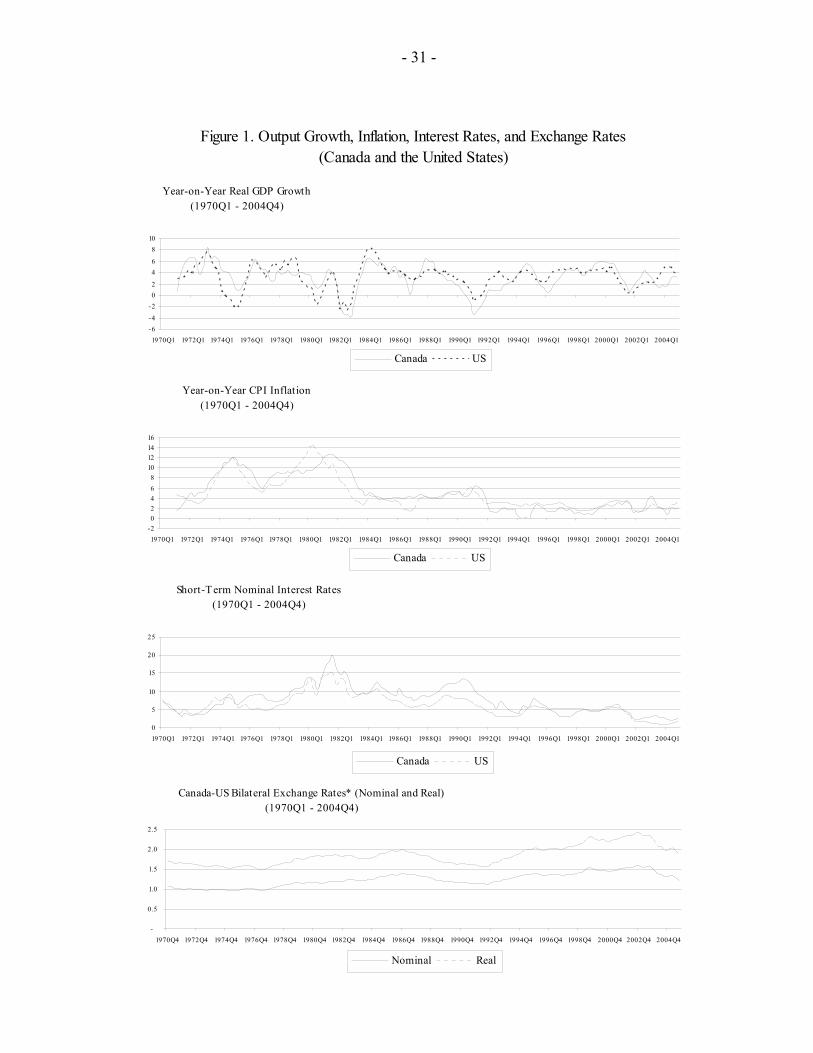
- 31 -

Figure 1. Output Growth, Inflation, Interest Rates, and Exchange Rates(Canada and the United States)

Year-on-Year Real GDP Growth(1970Q1 - 2004Q4)

-6-4

-202

46

810

1970Q1 1972Q1 1974Q1 1976Q1 1978Q1 1980Q1 1982Q1 1984Q1 1986Q1 1988Q1 1990Q1 1992Q1 1994Q1 1996Q1 1998Q1 2000Q1 2002Q1 2004Q1

Canada US

Year-on-Year CPI Inflation (1970Q1 - 2004Q4)

-202468

10121416

1970Q1 1972Q1 1974Q1 1976Q1 1978Q1 1980Q1 1982Q1 1984Q1 1986Q1 1988Q1 1990Q1 1992Q1 1994Q1 1996Q1 1998Q1 2000Q1 2002Q1 2004Q1

Canada US

Short-Term Nominal Interest Rates(1970Q1 - 2004Q4)

0

5

10

15

20

25

1970Q1 1972Q1 1974Q1 1976Q1 1978Q1 1980Q1 1982Q1 1984Q1 1986Q1 1988Q1 1990Q1 1992Q1 1994Q1 1996Q1 1998Q1 2000Q1 2002Q1 2004Q1

Canada US

Canada-US Bilateral Exchange Rates* (Nominal and Real)(1970Q1 - 2004Q4)

-

0.5

1.0

1.5

2.0

2.5

1970Q4 1972Q4 1974Q4 1976Q4 1978Q4 1980Q4 1982Q4 1984Q4 1986Q4 1988Q4 1990Q4 1992Q4 1994Q4 1996Q4 1998Q4 2000Q4 2002Q4 2004Q4

Nominal Real

- 32 -

Figure 2. Model Variables for Canada (Actual, Trend, and Detrended Series)

* An increase denotes a real depreciation

CANADA log of GDP (solid=actual, dashed=trend)

5.5

6

6.5

7

7.5

CANADAGDP (gap)

-6.0

-5.0

-4.0

-3.0

-2.0

-1.0

0.0

1.0

2.0

3.0

4.0

1970Q1 1975Q1 1980Q1 1985Q1 1990Q1 1995Q1 2000Q1

CANADA Real Interest Rate (solid=actual, dashed=trend)

-8

-6

-4

-2

0

2

4

6

8

10

12

1970Q1 1975Q1 1980Q1 1985Q1 1990Q1 1995Q1 2000Q1

CANADA Real Interest Rate (gap)

-12

-10

-8

-6

-4

-2

0

2

4

6

8

10

1970Q1 1975Q1 1980Q1 1985Q1 1990Q1 1995Q1 2000Q1

CANADA Real Exchange Rate* (solid=actual,

dashed=trend)

0

10

20

30

40

50

60

70

80

90

100

1970Q1 1975Q1 1980Q1 1985Q1 1990Q1 1995Q1 2000Q1

CANADA Real Exchange Rate (gap)

-15.0

-10.0

-5.0

0.0

5.0

10.0

15.0

1970Q1 1975Q1 1980Q1 1985Q1 1990Q1 1995Q1 2000Q1

- 33 -

Figure 3. Model Variables for the United States (Actual, Trend, and Detrended Series)

US log o f GDP (solid=actual, dashed=trend)

8

8.2

8.4

8.6

8.8

9

9.2

9.4

1970Q1 1975Q1 1980Q1 1985Q1 1990Q1 1995Q1 2000Q1

USGDP (gap)

-8 .0

-6 .0

-4 .0

-2 .0

0 .0

2 .0

4 .0

6 .0

1970Q1 1975Q1 1980Q1 1985Q1 1990Q1 1995Q1 2000Q1

US Real Interest Rate (solid=actual, dashed=trend)

-6

-4

-2

0

2

4

6

8

10

1970Q1 1975Q1 1980Q1 1985Q1 1990Q1 1995Q1 2000Q1

US Real Interest Rate (gap)

-8

-6

-4

-2

0

2

4

6

8

1970Q1 1975Q1 1980Q1 1985Q1 1990Q1 1995Q1 2000Q1

- 34 -

Figure 4. Dynamic Responses of Output, Inflation, and Short-Term Interest Rates in Canada100-basis-point rise in the policy rate for one quarter

(shock-minus-control responses for Canada)Comparing SMPMOD and the Bank of Canada Model (QPM)

-0.15

-0.10

-0.05

0.00

0.05

0.10

2005q

1

2005q

2

2005q

3

2005q

4

2006q

1

2006q

2

2006q

3

2006q

4

2007q

1

2007q

2

2007q

3

2007q

4

2008q

1

2008q

2

2008q

3

2008q

4

2009q

1

2009q

2

2009q

3

2009q

4

SMPMOD Core Inflation (year-on-year)

Bank of Canada QPM Core Inflation (year-on-year)

-0.40

-0.30

-0.20

-0.10

0.00

0.10

0.20

2005q

1

2005q

2

2005q

3

2005q

4

2006q

1

2006q

2

2006q

3

2006q

4

2007q

1

2007q

2

2007q

3

2007q

4

2008q

1

2008q

2

2008q

3

2008q

4

2009q

1

2009q

2

2009q

3

2009q

4

SMPMOD output gap Bank of Canada QPM output gap

-0.40-0.200.000.200.400.600.801.001.201.40

2005q

1

2005q

2

2005q

3

2005q

4

2006q

1

2006q

2

2006q

3

2006q

4

2007q

1

2007q

2

2007q

3

2007q

4

2008q

1

2008q

2

2008q

3

2008q

4

2009q

1

2009q

2

2009q

3

2009q

4

SMPMOD short-term interest rate Bank of Canada QPM short-term interest rate

- 35 -

Figure 5. Dynamic Responses of Output, Inflation , and Short-Term Interest Rates in the United States

100-basis-point rise in the policy rate for four quarters(shock-minus-control responses for the United States)

-2-1.5

-1-0.5

00.5

11.5

2005q

1

2005q

2

2005q

3

2005q

4

2006q

1

2006q

2

2006q

3

2006q

4

2007q

1

2007q

2

2007q

3

2007q

4

2008q

1

2008q

2

2008q

3

2008q

4

2009q

1

2009q

2

2009q

3

2009q

4

SMPMOD short-term interest rate FRBUS short-term interest rate

-0.6

-0.4

-0.2

0

0.2

0.4

0.6

2005q

1

2005q

2

2005q

3

2005q

4

2006q

1

2006q

2

2006q

3

2006q

4

2007q

1

2007q

2

2007q

3

2007q

4

2008q

1

2008q

2

2008q

3

2008q

4

2009q

1

2009q

2

2009q

3

2009q

4

SMPMOD output gap FRBUS output gap

-0.6

-0.5

-0.4

-0.3

-0.2

-0.1

0

2005q

1

2005q

2

2005q

3

2005q

4

2006q

1

2006q

2

2006q

3

2006q

4

2007q

1

2007q

2

2007q

3

2007q

4

2008q

1

2008q

2

2008q

3

2008q

4

2009q

1

2009q

2

2009q

3

2009q

4

SMPMOD core inflation (year-on-year) FRBUS core inflation (year-on-year)

- 36 - Ta

ble

1. B

asel

ine

Fore

cast

with

Des

k Ju

dgm

ent –

WEO

Sce

nario

20

03q1

2003

q220

03q3

2003

q420

04q1

2004

q220

04q3

2004

q420

05q1

2005

q220

05q3

200

5q4

2006

q120

06q2

2006

q320

06q4

2007

q120

07q2

2007

q320

07q4

Shor

t-T

erm

Inte

rest

Rat

es

Can

ada

2.9

3.2

2.8

2.7

2.2

22.

22.

52.

62.

72.

9 3.

23.

53.

84.

14.

34.

54.

74.

74.

7U

nite

d St

ates

1.

21.

11

0.9

0.9

1.1

1.5

1.8

22.

53

3.5

44.

54.

84.

84.

84.

84.

84.

8D

iffer

entia

l 1.

72.

11.

81.

71.

30.

90.

70.

80.

60.

2-0

.1

-0.3

-0.5

-0.7

-0.7

-0.4

-0.2

-0.1

00

Exc

hang

e R

ates

Val

ue o

f US

Dol

lar

(in C

anad

ian$

)

Lev

el

1.50

91.

397

1.38

1.31

61.

318

1.36

1.30

81.

219

1.22

11.

222

1.22

1.

217

1.21

31.

211.

207

1.20

51.

203

1.20

11.

198

1.19

4%

y-o

-y

-5.3

-10.

1-1

1.7

-15.

9-1

2.7

-2.6

-5.3

-7.4

-7.3

-10.

2-6

.7

-0.2

-0.7

-1-1

-0.9

-0.8

-0.7

-0.8

-0.9

% q

-o-q

-1

3.6

-26.

6-4

.7-1

7.4

0.6

13.6

-14.

6-2

4.6

0.8

0.3

-0.5

-1

.2-1

.2-0

.9-0

.8-0

.8-0

.7-0

.7-1

-1.2

Val

ue o

f Can

adia

n D

olla

r (in

US$

)

Lev

el

0.66

30.

716

0.72

50.

760.

759

0.73

50.

765

0.82

10.

819

0.81

90.

82

0.82

20.

825

0.82

60.

828

0.83

0.83

10.

833

0.83

50.

837

Rea

l Exc

hang

e R

ate

Gap

Can

ada

8.72

2.5

2.4

-1.6

80

3.94

0.81

-5.5

3-4

.61

-4.0

5-3

.7

-3.5

4-3

.37

-3.1

4-2

.92

-2.7

1-2

.5-2

.32

-2.2

3-2

.23

Rea

l GD

P G

row

th

Can

ada

%

y-o

-y

3.1

21.

31.

71.

62.

83.

33.

13.

12.

82.

7 2.

92.

93

3.1

3.1

3.2

3.2

3.1

3.1

% q

-o-q

2.

8-0

.71.

43.

32.

73.

93.

22.

52.

82.

82.

9 3

33.

13.

33.

23.

23.

13.

13

Uni

ted

Stat

es

%

y-o

-y

1.9

2.3

3.5

4.4

54.

84

3.7

3.6

3.7

3.6

3.8

3.7

3.7

3.7

3.7

3.7

3.7

3.6

3.6

% q

-o-q

1.

94.

17.

44.

24.

53.

34

3.1

3.8

3.8

3.7

3.7

3.6

3.7

3.7

3.6

3.6

3.6

3.6

3.5

CPI

Infla

tion

Can

ada

%

y-o

-y

4.4

2.8

2.1

1.7

0.8

2.2

22.

32.

52.

12.

4 2.

22.

12.

12.

12

22

22

% q

-o-q

4.

8-1

.61.

82

1.3

3.8

12.

92.

22.

42

2.2

22

22

22

22

Uni

ted

Stat

es

%

y-o

-y

2.9

2.2

2.2

1.9

1.8

2.8

2.7

3.4

3.2

2.7

2.7

2.4

2.3

2.3

2.4

2.5

2.5

2.5

2.5

2.5

% q

-o-q

3.

90.

62.

30.

73.

64.

71.

93.

43

2.4

2 2.

42.

42.

52.

52.

52.

52.

52.

52.

5C

ore

CPI

Infla

tion

Can

ada

%

q-o

-q

3.1

2.2

1.7

1.9

1.3

1.7

1.7

1.6

1.9

1.9

2.1

2.2

2.1

2.1

2.1

22

22

2U

nite

d St

ates

% y

-o-y

2.

11.

81.

51.

51.

31.

92.

83.

14.

13.

83.

1 2.

82.

32.

32.

42.

52.

52.

52.

52.

5Pr

ice

of O

il ($

)

Wor

ld m

arke

t 31

.326

.528

.429

.432

.135

.640

.642

.741

.341

40.3

39

.538

.838

.337

.837

.336

.836

.335

.835

.3O

utpu

t Gap

Can

ada

0.4

-0.4

-0.8

-0.7

-0.7

-0.4

-0.3

-0.4

-0.4

-0.3

-0.3

-0

.3-0

.3-0

.2-0

.10

00.

10.

10.

1U

nite

d St

ates

-3

.3-3

.1-2

.2-2

-1.7

-1.7

-1.5

-1.6

-1.4

-1.3

-1.2

-1

.1-1

-0.9

-0.7

-0.6

-0.5

-0.4

-0.3

-0.2

Pote

ntia

l Out

put G

row

th (%

q-o

-q)

C

anad

a 2.

92.

82.

82.

82.

82.

82.

82.

82.

82.

82.

8 2.

82.

92.

92.

92.

92.

92.

92.

92.

9U

nite

d St

ates

3.

43.

43.

43.

43.

43.

33.

33.

33.

33.

23.

2 3.

23.

23.

23.

23.

23.

23.

23.

23.

2M

odel

Res

idua

ls a

nd J

udgm

ent

Can

ada

In

flatio

n 1.

6-4

.6-0

.20.

5-0

.62.

1-1

.21.

50.

20.

20

0.2

0.1

0.1

0.1

0.1

0.1

0.1

0.1

0.1

Cor

e In

flatio

n 0.

4-2

-0.7

0.8

-0.9

1.3

-0.5

0.3

0.5

0.4

0.1

0.2

-0.1

00

00

00

0O

utpu

t Gap

-0

.1-0

.20

0.3

0.3

0.2

0.1

00.

40.

30.

3 0.

30.

30.

30.

30.

30.

30.

30.

20.

2N

omin

al In

tere

st R

ate

-1-0

.7-0

.8-0

.6-0

.8-1

.4-1

.2-1

.0-1

.2-0

.9-0

.8

-0.5

-0.4

-0.2

-0.1

0.1

0.1

0.1

0.1

0.1

Rea

l Exc

hang

e R

ate

(per

cent

age

poin

ts)

6.5

-13.

74.

4-1

1.8

-5.7

13.4

5-1

5.5

-1-1

.5-1

.5

-1.8

-1.9

-1.8

-1.6

-1.3

-0.9

-0.6

-0.4

-0.4

Uni

ted

Stat

es

In

flatio

n 2.

2-1

.21.

3-1

.31.

72.

8-0

.90.

80.

3-0

.1-0

.1

0.2

0.4

0.6

0.5

0.4

0.3

0.3

0.2

0.2

Out

put G

ap

-1.0

-0.3

0.3

-0.2

-0.3

-0.7

-0.2

-0.5

-0.3

-0.2

-0.1

-0

.1-1

.0-0

.00.

00.

00.

00.

.10.

00.

0N

omin

al In

tere

st R

ate

-0.3

-0.8

-1.5

-1.8

-2.2

-2.1

-1.5

-1.5

-1-0

.4-0

.3

00.

30.

50.

40.

20.

20.

20.

10.

1O

il eq

uatio

n (p

erce

ntag

e po

ints

) 12

-16.

62

0.1

5.4

8.2

13.6

8.2

0.6

2.5

1.0

0.3

-0.2

-0.1

-0.5

-0.8

-1.0

-1.3

-1.6

-1.8

- 37 -

Table 2. Canada: Canadian Interest Rate Shock – One Quarter Increase of 100 b.p. Summary Table

Deviations from a WEO Baseline (percent deviation) or [percentage point deviation]

Quarterly Annual

2004 2005

Q1 Q2 Q3 Q4 Q1 Q2 Q3 Q4 2003 2004 2005 2006 2007 2008 2009

Short-term Interest Rate 2.2 2.0 2.2 2.5 3.6 3.0 2.9 3.0 2.9 2.2 3.1 3.7 4.6 4.8 4.8 [ +1.0] [ +0.4] [ +0.0] [ -0.2] [ +0.3] [ -0.3] [ -0.1] [ +0.1] [ +0.1]

Value of C$ (in US$) 0.759 0.735 0.765 0.821 0.823 0.822 0.821 0.821 0.716 0.770 0.822 0.823 0.832 0.847 0.851 ( +0.5) ( +0.4) ( +0.1) ( -0.2) ( +0.2) ( -0.5) ( -0.2) ( +0.4) ( +0.5)

Real GDP Growth

% y-o-y 1.6 2.8 3.3 3.1 3.1 2.7 2.5 2.7 2.0 2.7 2.7 3.1 3.4 2.9 2.8 [ -0.0] [ -0.2] [ -0.2] [ -0.2] [ -0.2] [ +0.1] [ +0.2] [ -0.0] [ -0.1]

% q-o-q 2.7 3.9 3.2 2.5 2.7 2.2 2.6 3.1 [ -0.1] [ -0.6] [ -0.2] [ +0.0]

CPI Inflation

% y-o-y 0.85 2.22 2.02 2.25 2.47 2.10 2.34 2.15 2.74 1.83 2.27 1.99 1.94 2.00 2.05 [ -0.02] [ -0.03] [ -0.04] [ -0.06] [ -0.03] [ -0.08] [ -0.08] [ -0.02] [+0.02]

% q-o-q 1.31 3.84 0.97 2.92 2.17 2.37 1.90 2.15 [ -0.07] [ -0.03] [ -0.05] [ -0.07]

Core CPI Inflation 1.31 1.69 1.66 1.57 1.93 1.90 2.07 2.14 2.21 1.56 2.01 1.96 1.94 2.03 2.07 % y-o-y [ -0.01] [ -0.02] [ -0.04] [ -0.06] [ -0.03] [ -0.11] [ -0.08] [+0.01] [+0.04] 0.76 2.51 1.19 1.83 2.21 2.37 1.87 2.11 % q-o-q [ -0.03] [ -0.03] [ -0.08] [ -0.11]

Price of oil (US$) 32.1 35.6 40.6 42.7 41.3 41.0 40.3 39.5 28.9 37.8 40.5 38.0 36.0 35.0 34.5 ( -0.0) ( +0.0) ( +0.0) ( +0.0) ( +0.0) ( +0.0) ( +0.0) ( +0.0) ( -0.0)

Output Gap -0.67 -0.40 -0.29 -0.35 -0.37 -0.50 -0.55 -0.50 -0.36 -0.43 -0.48 -0.22 0.23 0.23 0.03 [ -0.02] [ -0.16] [ -0.22] [ -0.21] [ -0.15] [ -0.07] [+0.14] [+0.13] [ -0.00]

Potential Output Growth % y-o-y 2.8 2.8 2.8 2.8 2.8 2.8 2.8 2.8 2.9 2.8 2.8 2.9 2.9 3.0 3.0 [ +0.0] [ +0.0] [ +0.0] [ +0.0] [ +0.0] [ -0.0] [ -0.0] [ +0.0] [ +0.0] % q-o-q 2.8 2.8 2.8 2.8 2.8 2.8 2.8 2.8

[ +0.0] [ +0.0] [ +0.0] [ +0.0]

- 38 -

Table 3. United States: U.S. Interest Rate Shock – One Quarter Increase of 100 b.p. Summary Table

Deviations from a WEO Baseline (percent deviation) or [percentage point deviation]

Quarterly Annual

2004 2005

Q1 Q2 Q3 Q4 Q1 Q2 Q3 Q4 2003 2004 2005 2006 2007 2008 2009

Short-term Interest Rate 0.9 1.1 1.5 1.8 3.0 2.9 3.0 3.3 1.0 1.3 3.0 4.1 4.4 4.6 4.8 [ +1.0] [ +0.4] [ -0.0] [ -0.2] [ +0.3] [ -0.4] [ -0.3] [ -0.1] [ +0.1]

Value of C$ (in US$) 0.759 0.735 0.765 0.821 0.814 0.813 0.815 0.819 0.716 0.770 0.816 0.828 0.835 0.845 0.848 ( -0.6) ( -0.7) ( -0.5) ( -0.3) ( -0.5) ( +0.1) ( +0.2) ( +0.2) ( +0.2) Real GDP Growth

% y-o-y 5.0 4.8 4.0 3.7 3.5 3.6 3.4 3.6 3.0 4.4 3.5 3.7 3.8 3.6 3.3

[ -0.0] [ -0.1] [ -0.2] [ -0.2] [ -0.1] [ +0.0] [ +0.1] [ +0.1] [ -0.0]

% q-o-q 4.5 3.3 4.0 3.1 3.7 3.3 3.6 3.7 [ -0.1] [ -0.5] [ -0.2] [ +0.0] CPI Inflation

% y-o-y 1.80 2.84 2.71 3.39 3.24 2.65 2.67 2.39 2.27 2.69 2.74 2.27 2.36 2.41 2.49 [ -0.00] [ -0.01] [ -0.03] [ -0.06] [ -0.03] [ -0.12] [ -0.14] [ -0.09] [ -0.01]

% q-o-q 3.58 4.73 1.85 3.42 2.98 2.37 1.92 2.29

Core CPI Inflation [ -0.02] [ -0.03] [ -0.08] [ -0.11]

% y-o-y 1.29 1.87 2.84 3.12 4.07 3.79 3.09 2.74 1.73 2.28 3.42 2.24 2.36 2.41 2.49 [ -0.00] [ -0.01] [ -0.03] [ -0.06] [ -0.03] [ -0.12] [ -0.14] [ -0.09] [ -0.01]

% q-o-q 0.72 3.58 4.73 3.50 4.48 2.47 1.92 2.09 [ -0.02] [ -0.03] [ -0.08] [ -0.11] Price of oil (US$) 32.1 35.6 40.6 42.7 41.2 41.0 40.2 39.5 28.9 37.8 40.5 37.9 35.9 34.9 34.4 ( -0.0) ( -0.0) ( -0.0) ( -0.1) ( -0.0) ( -0.1) ( -0.3) ( -0.4) ( -0.4)

Output Gap -1.69 -1.70 -1.53 -1.56 -1.45 -1.43 -1.35 -1.23 -2.63 -1.62 -1.37 -0.89 -0.34 0.03 0.15 [ -0.01] [ -0.13] [ -0.17] [ -0.17] [ -0.12] [ -0.09] [+0.04] [+0.10] [+0.09]

Potential Output Growth % y-o-y 3.4 3.4 3.3 3.3 3.3 3.3 3.3 3.2 3.4 3.3 3.3 3.2 3.2 3.2 3.2 [ +0.0] [ +0.0] [ +0.0] [ +0.0] [ +0.0] [ +0.0] [ +0.0] [ +0.0] [ +0.0]% q-o-q 3.4 3.3 3.3 3.3 3.3 3.2 3.2 3.2 [ +0.0] [ +0.0] [ +0.0] [ +0.0]

- 39 -

REFERENCES

Bayoumi, T., and S. Sgherri, 2004, “Monetary Magic? How the Fed Improved Flexibility of the Economy,” CEPR Discussion Paper No. 4696 (London: Centre for Economic Policy Research).

Berg, A., C. Jarvis, M. Stone, and A. Zanello, 2003, "Re-Establishing Credible Nominal Anchors

after a Financial Crisis: A Review of Recent Experience" in Managing Financial Crises: Recent Experience and Lessons for Latin America, ed. by Charles Collyns and Russell Kincaid, IMF Occasional Paper No. 217 (Washington: International Monetary Fund)

Berg, A., P. Karam, and D. Laxton, 2006, “A Practical Model-Based Approach to Monetary Policy

Analysis—How-to-Guide,” IMF Working Paper 06/81 (Washington: International Monetary Fund).

Blanchard, O., and S. Fischer, 1989, Macroeconomics (Cambridge, Massachusetts: MIT Press). Blejer, M., A. Leone, P. Rabanal, and G. Schwartz, 2001, "Inflation Targeting in the Context of

IMF-Supported Adjustment Programs," in Ten Years of Inflation Targeting: Design, Performance, Challenges, ed. by N. Loayza and R. Soto (Santiago: Central Bank of Chile).

Bofinger, P., and R. Schmidt, 2004, "Should One Rely on Professional Exchange Rate Forecasts?

An Empirical Analysis of Professional Forecasts for the Euro/US$ Rate," CEPR Discussion Paper No. 4235 (London: Centre for Economic Policy Research).

Botman, D., D. Muir, D. Laxton, and A. Romanov, 2006, “A New-Open-Economy-Macro Model

for Fiscal Policy Evaluation” (unpublished, Washington: International Monetary Fund). Canales-Kriljenko, Jorge Evan, Turgut Kisinbay, Rodolfo Maino, and Eric Parrado, 2006, “Setting

the Operational Framework for [Inflation Targeting],” IMF working paper, forthcoming (Washington: International Monetary Fund).

Cespedes L., M. Kumhof, and E. Parrado, 2003, “Pricing Policies and inflation inertia,” IMF

Working Paper 03/87 (Washington: International Monetary Fund). Chin, M., and G. Meredith, 1998, “Long-Horizon Uncovered Interest Rate Parity,” NBER Working

Paper No. 6797 (Cambridge, Massachusetts: National Bureau of Economic Research). Choi, W. G., and Y. Jung, 2003, "Optimal Monetary Policy in a Small Open Economy with Habit

Formation and Nominal Rigidities," IMF Working Paper 03/5 (Washington: International Monetary Fund).

Clarida, R., J. Gali, and M. Gertler, 1999, "The Science of Monetary Policy: A New Keynesian

Perspective," Journal of Economic Literature, Vol. 37, No. 4, pp. 1661–707. Coats, W., D. Laxton, and D. Rose, 2003, The Czech National Bank’s Forecasting and Policy

Analysis System, (Prague: Czech National Bank).

- 40 -

Coletti, D., B. Hunt, D. Rose, and R. Tetlow, 1996, "Bank of Canada's New Quarterly Projection Model. Part 3, The Dynamic Model: QPM," Bank of Canada Technical Report No. 75 (Ottawa: Bank of Canada).

Cozier, B. and G. Wilkinson, 1990, "How Large Are the Costs of Disinflation in Canada," Bank of

Canada Working Paper No. 90-6 (Ottawa: Bank of Canada). Debelle, G., 2000, “Inflation Targeting and Output Stabilization in Australia,” ed. by M. Blejer,

A. Ize, A. Leone, and S. Werlang, in Inflation Targeting in Practice (Washington: International Monetary Fund).

Eggertsson, Gauti and Michael Woodford, 2003, “The Zero Bound on Interest Rates and Optimal

Monetary Policy," Brookings Papers on Economic Activity 2003:1, pp. 139-211. Elekdag, S. and I. Tchakarov, 2004, “Balance Sheet Effects, Exchange Rate Policy and Welfare,”

IMF Working Paper 04/63 (Washington: International Monetary Fund). Epstein, N., P. Karam, D. Laxton, and D. Rose, 2006, “A Simple Forecasting and Policy Analysis

System for Israel: Structure and Applications,” in Israel: Selected Issues, ed. by Rick Haas, Country Report No. 06/121 (Washington: International Monetary Fund), available at http://www.imf.org/external/pubs/cat/longres.cfm?sk=19088.0

Erceg, C. and A. Levin, 2001, "Imperfect Credibility and Inflation Persistence," Working Paper,

Board of Governors of the Federal Reserve System (Washington: U.S. Federal Reserve). Faust, J., E. Swanson, and J. Wright, 2004, “Identifying VARS based on high frequency futures

data,” Journal of Monetary Economics, Vol. 51 (September), pp. 1107-1131. Faust, J., and C. Whiteman, 1997, “General-to-Specific Procedures for Fitting a Data-Admissible,

Theory-Inspired, Congruent, Parsimonious, Encompassing, Weakly-Exogenous, Identified, Structural Model to the DGP: A Translation and Critique,” Carnegie-Rochester Conference Series on Public Policy, Vol. 47 (December), pp. 121-126.

Friedman, Benjamin, 2003, “The LM Curve: A Not-So-Fond Farewell”, NBER Working Paper

No. 10123 (Cambridge: National Bureau of Economic Research). Gali, J. and T. Monacelli, 2002, “Monetary Policy and Exchange Rate Volatility in a Small Open

Economy,” NBER Working Paper No. 8905, pp. 1-43 (Cambridge, Massachusetts: National Bureau of Economic Research).

Garratt, A., K. Lee, H. Pesaran, and Y. Shin, 2003, “A Long Run Structural Macroeconometric

Model of the UK,” The Economic Journal, Vol. 113 (April), pp. 412 – 27. Gueorguiev, N., 2003, “Exchange Rate Pass-Through in Romania,” IMF Working Paper

03/130 (Washington: International Monetary Fund).

- 41 -

Ho, C., and R. McCauley, 2003, “Living with Flexible Exchange Rates: Issues and Recent Experience in Inflation Targeting Emerging Market Economies,” BIS Working Paper No. 130 (Basel, Switzerland: Bank for International Settlements).

Hunt, B., 2005, “Oil Price Shocks: Can They Account for the Stagflation in the 1970s?” IMF

Working Paper (forthcoming; Washington: International Monetary Fund). Hunt, B., D. Rose, and A. Scott, 2000, "The Core Model of the Reserve Bank of New Zealand's

Forecasting and Policy System," Economic Modelling, Vol. 17, pp. 247-74. Hunt, B., and A. Orr, 1999, Monetary Policy Under Uncertainty, Reserve Bank of New Zealand

Conference Volume (Wellington: Reserve Bank of New Zealand). Hunt, B., P. Isard, and D. Laxton, 2003, “Inflation Targeting and the Role of the Exchange Rate,”

(unpublished, Washington: International Monetary Fund) Hunt, B., Robert Tchaidze, and Ann-Margret Westin, 2005, Iceland: Selected Issues, Country Report

No. 05/366 (Washington: International Monetary Fund), available at http://www.imf.org/external/pubs/cat/longres.cfm?sk=18623.0.

International Monetary Fund, 2004a, “Policy Formulation, Analytic Frameworks, and Program

Design,”, prepared by the Policy Development and Review Department, (Washington: International Monetary Fund), http://www.imf.org/external/np/pdr/2004/eng/policy.htm

———, 2004b, “Macroeconomic and Structural Policies in Fund-Supported Programs: Review of

Experience,”, prepared by the Policy Development and Review Department, IMF (Washington: International Monetary Fund), http://www.imf.org/external/np/pdr/2004/eng/design.htm

Isard, P., and B. Hunt, 2003, “Some Implications for Monetary Policy of Uncertain Passthrough,”

IMF Working Paper 03/25 (Washington: International Monetary Fund). Isard, P., and D. Laxton, 1998, “Monetary Policy with NAIRU Uncertainty and Endogenous

Credibility: Perspectives on Policy Rules and the Gains from Experimentation and Transparency,” in Monetary Policy Under Uncertainty, ed. by Benjamin Hunt and Adrain Orr, Reserve Bank of New Zealand Conference Volume, pp. 33-65 (Wellington: Reserve Bank of New Zealand).

———, 2000, “Issues Related to Inflation Targeting,” IMF Staff Country Report No. 00/106

(Washington: International Monetary Fund). Juillard, M., P. Karam, D. Laxton, and P. Pesenti, 2005, “A Simple Welfare-Based Monetary Policy

Rule in an Estimated DSGE Model of the US Economy,” European Central Bank Working Paper. (forthcoming; Frankfurt: European Central Bank). Also available at http://www.ny.frb.org/research/economists/pesenti/jukalape.pdf.

- 42 -

Kapetanios, G., A. Pagan, and A. Scott, 2005, “Making a Match: Combining Theory and Evidence in Policy-Oriented Macroeconomic Modeling,” Centre for Applied Macroeconomic Analysis Working Paper No. 2005-1 (Canberra Australian National University).

Lane, P., 2001, "The New Open Economy Macroeconomics: A Survey," Journal of International

Economics (August).

Laxton, D., and P. N'Diaye, 2002, "Monetary Policy Credibility and the Unemployment-Inflation Tradeoff: Some Evidence from 17 Industrial Countries," IMF Working Paper 02/220 (Washington: International Monetary Fund).

Laxton, D., and P. Pesenti, 2003,"Monetary Policy Rules for Small, Open, Emerging Economies,"

Journal of Monetary Economics, Vol. 50 (July), pp. 1109-46.

Laxton, D., and A. Scott, 2000, "On Developing a Structured Forecasting and Policy Analysis System Designed to Support Inflation-Forecast Targeting (IFT)," in Inflation Targeting Experiences: England, Finland, Poland, Mexico, Brazil, Chile (Ankara: The Central Bank of the Republic of Turkey), pp. 6-63.

Leeper, E., 2003, "An Inflation Reports Report," Sveriges Riksbank Economic Review No. 3,

pp. 94-118. ________, and J. Roush, 2003, "Putting 'M' Back in Monetary Policy," NBER Working Paper No.

9552 (Cambridge Massachusetts: National Bureau of Economic Research). Leigh, D., 2005, “Estimating the Implicit Inflation Target: An Application to U.S. Monetary Policy,”

IMF Working Paper 05/77 (Washington: International Monetary Fund). Monacelli, T., 2004, “Into the Mussa Puzzle: Monetary Policy Regimes and the Real Exchange Rate

in a Small Open Economy,” Journal of International Economics, Vol. 62, pp. 191-217. Murchison S., 2001, "NAOMI, A New Quarterly Model. Part II: A Guide to Canadian NAOMI,"

Department of Finance Working Paper No. 2001/25 (Ottawa: Department of Finance). __________, 2004, “Exchange Rate Pass-through and Monetary Policy: How Strong Is the Link?,

Bank of Canada Working Paper (Ottawa: Bank of Canada). Mussa, M., and M. Savastano, 2000, "The IMF Approach to Economic Stabilization." in NBER

Macroeconomics Annual 1999, ed. by B. Bernanke and J. Rotemberg, (Cambridge, Massachusetts: MIT Press), pp. 79-122.

Orphanides, A., 2003, "Historical Monetary Policy Analysis and the Taylor Rule." Journal of

Monetary Economics, Vol. 50, pp. 983-1022.

- 43 -

Parrado, E., 2004, “Inflation Targeting and Exchange Rate Rules in an Open Economy,” IMF Working Paper 04/21 (Washington: International Monetary Fund).

Romer, C.D., and D.H. Romer, 2000, “Federal Reserve Information and the Behavior of Interest

Rates,” American Economic Review, Vol. 90 (3), pp. 429-457. Romer, D., 2000, "Keynesian Macroeconomics without the Lm Curve," Journal of Economic

Perspectives, Vol. 14, Issue 2 (Spring), pp. 149-69.

Rudebusch, Glenn D., 2002, “Term Structure Evidence on Interest Rate Smoothing and Monetary Policy Inertia,” Journal of Monetary Economics, Vol. 49, pp. 1161–87.

Schmidt-Hebbel, K., and M. Tapia, 2002, “Monetary Policy Implementation and Results in Twenty

Inflation Targeting Countries,” Working Paper No. 166 (Santiago: Central Bank of Chile). Sims, C., 2002, “The Role of Models and Probabilities in the Monetary Policy Process,” Brookings

Papers on Economic Activity, 2. Smets, F., and R. Wouters, 2004, "Comparing Shocks and Frictions in US and Euro Area Business

Cycles: A Bayesian DSGE Approach." European Central Bank Working Paper, No. 391 (September) (Frankfurt: European Central Bank).

Stiglitz, J., and C. Walsh, 2002, Principles of Macroeconomics, (New York: W.W. Norton, 3rd ed.). Stone, M., and A. Bhundia, 2004, “A New Taxonomy of Monetary Regimes,” IMF Working

Paper 04/191 (Washington: International Monetary Fund). Svensson, L., and R. Tetlow, 2005, “Optimal Policy Projections,” International Journal of Central

Banking, Vol. 1(3), pp. 177-207. Taylor, J., 1999, Monetary Policy Rules (Chicago: University of Chicago Press).

Truman, E., 2003, Inflation Targeting in the World Economy (Washington: Institute for International

Economics). Woodford, M., 2001, “Imperfect Common Knowledge and the Effects of Monetary Policy,”

ed. by P. Aghion, R. Frydman, J. Stiglitz, and M. Woodford, in Knowledge, Information and Expectations in Modern Macroeconomics: In Honor of Edmund S. Phelps (Princeton, New Jersey: Princeton University Press).

_________, 2003a, Interest and Prices: Foundations of a Monetary Theory (Princeton: Princeton

University Press). ________, 2003b, "Optimal Monetary Policy Inertia," Review of Economic Studies, Vol. 70,

pp. 861-86.