hpfbench: a high performance fortran benchmark suiteychu/publications/hpfbench.pdf · ......

HPFBench: A High Performance FortranBenchmark Suite

Y. CHARLIE HUHarvard UniversityGUOHUA JINRice UniversityandS. LENNART JOHNSSON, DIMITRIS KEHAGIAS, and NADIA SHALABYHarvard University

The High Performance Fortran (HPF) benchmark suite HPFBench is designed for evaluatingthe HPF language and compilers on scalable architectures. The functionality of the bench-marks covers scientific software library functions and application kernels that reflect thecomputational structure and communication patterns in fluid dynamic simulations, funda-mental physics, and molecular studies in chemistry and biology. The benchmarks are charac-terized in terms of FLOP count, memory usage, communication pattern, local memoryaccesses, array allocation mechanism, as well as operation and communication counts periteration. The benchmarks output performance evaluation metrics in the form of elapsedtimes, FLOP rates, and communication time breakdowns. We also provide a benchmark guideto aid the choice of subsets of the benchmarks for evaluating particular aspects of an HPFcompiler. Furthermore, we report an evaluation of an industry-leading HPF compiler from thePortland Group Inc. using the HPFBench benchmarks on the distributed-memory IBM SP2.

Categories and Subject Descriptors: D.3.2 [Programming Languages]: Language Classifica-tions—Concurrent, distributed, and parallel languages; G.1.3 [Numerical Analysis]: Numer-ical Linear Algebra—Linear systems (direct and iterative methods); G.4 [Mathematics of

The programs in HPFBench suite were developed by Thinking Machines Corp. in ConnectionMachine Fortran with partial support from ARPA under subcontract DABT63-91-C-0031 withthe Computer Science Department of Yale University and the Northeast Parallel Architec-tures Center (NPAC) at Syracuse University. Verification, debugging, and documentationwere made in part by the Parallel Computation Research Group at Harvard University withsupport from Thinking Machines Corp. Porting to High Performance Fortran was partiallysupported by the Computer Science Department and the Center for Research and ParallelComputation of Rice University.Authors’ addresses: Y. C. Hu, Division of Engineering and Applied Sciences, Harvard Univer-sity, 33 Oxford Street, Cambridge, MA 02138; G. Jin, Computer Science Department, RiceUniversity, 6100 Main Street, Houston, TX 77005; S. L. Johnsson, D. Kehagias, and N.Shalaby, Division of Engineering and Applied Sciences, Harvard University, 33 Oxford Street,Cambridge, MA 02138.Permission to make digital / hard copy of part or all of this work for personal or classroom useis granted without fee provided that the copies are not made or distributed for profit orcommercial advantage, the copyright notice, the title of the publication, and its date appear,and notice is given that copying is by permission of the ACM, Inc. To copy otherwise, torepublish, to post on servers, or to redistribute to lists, requires prior specific permissionand / or a fee.© 2000 ACM 0098-3500/00/0300–0099 $5.00

ACM Transactions on Mathematical Software, Vol. 26, No. 1, March 2000, Pages 99–149.

Computing]: Mathematical Software—Efficiency; Parallel and vector implementations; I.6.3[Simulation and Modeling]: Applications; J.2 [Computer Applications]: Physical Sciencesand Engineering—Astronomy; Chemistry; J.3 [Computer Applications]: Life and MedicalSciences—Biology and genetics

General Terms: Languages, Measurement, Performance

Additional Key Words and Phrases: Benchmarks, compilers, High Performance Fortran

1. INTRODUCTIONHigh Performance Fortran (HPF) [High Performance Fortran Forum 1993;1997] is the first widely supported, efficient, and portable parallel program-ming language for shared- and distributed-memory systems. It continuesthe Fortran tradition of providing a balanced mix of features for writingportable but efficient programs, and is realized by defining a set ofstandard extensions to Fortran 90. High-level constructs such as FORALLare provided where advanced compilers are believed capable of generatingefficient code for different hardware. Programmer control (such as arraylayout directives) is provided in areas for which compiler optimizationremains a challenging problem. Thus, HPF enables application developersto write portable and efficient software that will compile and execute ontraditional vector multiprocessors, shared-memory machines, distributedshared-memory machines, message passing distributed-memory machines,and distributed systems, such as networks of workstations.

Since the first release of the HPF specification in 1994, a growingnumber of vendors have made commercially available HPF compilers, withmore vendors announcing plans to join the effort. However, there has notbeen a systematically designed HPF benchmark suite for evaluating thequalities of the HPF compilers, and the HPF compiler vendors have mostlyrelied on individual application programmers to feedback their experienceoften with some particular type of applications on a particular type ofarchitecture (for example, see Hu et al. [1997]). The development of theHPFBench benchmark suite was a first effort to produce a means forevaluating HPF compilers on all scalable architectures.

The functionality of the HPFBench benchmarks covers linear algebralibrary functions and application kernels. The motivation for includinglinear algebra library functions is for measuring the capability of compilersin compiling the frequently time-dominating computations in applications.

One motivation for building libraries, in particular in the early years ofnew architectures, is that they may offer significantly higher performanceby being implemented, at least in part, in lower-level languages to avoiddeficiencies in compiler technology, or in the implementation of compilersand run-time systems. However, though the functionality of libraries islimited compared to that of applications being run on most computers,implementing libraries in low-level languages tend to be very costly, andoften means that high or even good performance may not be available until

100 • Y. C. Hu et al.

ACM Transactions on Mathematical Software, Vol. 26, No. 1, March 2000.

late in the hardware product cycle. This in turn implies that following therapid advances in hardware technology is very difficult, since the oldergeneration hardware often competes successfully with the new generationbecause of the difference in the quality of software. Thus, it is important tominimize the amount of low-level code also in software libraries, and shiftthe responsibility of achieving high efficiency to the compiler.

In addition to some of the most common linear algebra functions that arefrequently occurring in many science and engineering applications, theHPFBench benchmark suite also contains a set of small application codescontaining typical “inner loop” constructs that are critical for performance,but that are typically not found in libraries. An example is stencil evalua-tions in explicit finite difference codes. The benchmarks were chosen tocomplement each other, such that a good coverage would be obtained oflanguage constructs and idioms frequently used in scientific applications,and for which high performance is critical for good performance of theentire application. Much of the resources at supercomputer centers areconsumed by codes used in fluid dynamic simulations, in fundamentalphysics, and in molecular studies in chemistry or biology. The selection ofapplication codes in the HPFBench benchmark suite reflects this fact.

The two groups of HPFBench are listed as follows. The names by whichwe refer to the codes are given in parenthesis.

Linear algebra library functions(1) Triangular solvers:

(a) Conjugate Gradient (conj-grad )(b) Parallel cyclic reduction (pcr )

(2) Fast Fourier transform (fft )(3) Gauss-Jordan matrix inversion (gauss-jordan )(4) Jacobi eigenanalysis (jacobi )(5) LU factorization (lu )(6) Matrix-Vector multiplication (matrix-vector )(7) QR factorization and solution (qr )

Applications kernels cover the following applications and methods:(1) Boson: many-body simulation (boson )(2) Diffusion equation: in three dimensions using an explicit finite

difference algorithm (diff-3d )(3) Poisson’s equation by the Conjugate Gradient method (ellip-2d )(4) Solution of the equilibrium equations in three dimensions by the

finite-element method (fem-3d )(5) Seismic processing: generalized moveout (gmo)(6) Spectral method: integration of Kuramoto-Sivashiniski equations

(ks-spectral )(7) Molecular dynamics, Leonard-Jones force law:

(a) with local forces only (mdcell )(b) with long-range forces (md)

(8) Generic direct N-body solvers with long-range forces (for vortices)(n-body )

HPFBench: A High Performance Fortran Benchmark Suite • 101


(9) Particle-in-cell in two dimensions:(a) straightforward implementation (pic-simple )(b) sophisticated implementation (pic-gather-scatter )

(10) QCD kernel: staggered fermion Conjugate Gradient method (qcd-kernel )

(11) Quantum Monte-Carlo (qmc)(12) Quadratic programming (qptransport )(13) Solution of nonsymmetric linear equations using the Conjugate

Gradient Method (rp )(14) Euler fluid flow in two dimensions using an explicit finite difference

scheme (step4 )(15) Wave propagation in one dimension (wave-1d )

The concept of measuring performance using benchmark codes is notnew. Earlier efforts on benchmarking supercomputer performance (see, forexample Wueller-Wichards and Gentzsch [1982], Lubeck et al. [1985], andDongarra et al. [1987]) focused on ad hoc approaches to the evaluation ofsystems rather than on potential standardization of the benchmark pro-cess. Later benchmarking efforts emphasized more on the methodology andmetrics applied to the evaluation of supercomputing systems. In particular,the well-known sets include the Livermore Fortran kernels [McMahon1988], the LINPACK [Dongarra 1989], and the NAS kernels from NASA/Ames [Bailey and Barton 1985]. Each of these benchmark sets containscodes that closely relate to one particular type of science and engineeringresearch in a particular environment. Furthermore, the benchmarks aremostly designed for measuring uniprocessors though the NAS parallelbenchmarks [Bailey et al. 1994] are “paper and pencil” benchmarks thatspecify the task to be performed and allow the implementor to choosealgorithms as well as programming model, and the newer NAS parallelbenchmarks 2.0 [Bailey et al. 1995] consists of MPI-based source imple-mentations. The Perfect Club benchmarks [Berry et. al. 1989; Cybenko etal. 1990; Sinvhal-Sharma et al. 1991] is a collection of Fortran 77 applica-tion codes originally designed for the evaluation of sequential architec-tures, though there have been efforts in porting the codes to parallelmachines [Cybenko et al. 1990]. Different from earlier benchmarks, thePerfect Club benchmarks focus on whole application codes from severalareas of engineering and scientific computing.

The benchmark package most closely related to HPFBench is the PARK-BENCH benchmark suite [Hockney and Berry 1994], which represents aninternational collaborative effort on providing a focused parallel machinebenchmarking activities and setting standards for benchmarking method-ologies. PARKBENCH suite defines four areas of benchmarking focus, andis collecting actual benchmarks from existing benchmarks suites or fromusers’ submissions. The programming models of the benchmark codes areplanned to be both message passing and HPF. The four benchmarkingfocuses include low-level benchmarks for measuring basic computer charac-teristics, kernel benchmarks to test typical scientific subroutines, compact

102 • Y. C. Hu et al.


applications to test complete problems, and HPF kernels to test thecapabilities of HPF compilers. The motivation for kernel benchmarks andcompact applications resembles that of the linear algebra functions andapplications kernels in our HPFBench suite, while the HPF kernels inPARKBENCH are for testing different phases of compilations rather thanbenchmarking whole HPF codes. At the release of the first PARKBENCHreport in 1994, the suite contained very few actual codes, and the compactapplications were largely missing. The HPFBench efforts were first startedin 1990 and therefore overlapped with the PARKBENCH effort. Further-more, to our knowledge, the HPFBench suite is the first benchmark suitethat focuses entirely on the High Performance Fortran programming envi-ronments.

In this article, we strive to provide sufficient insight into the benchmarkcodes for prospective users to choose one or a subset of codes that wouldbest expose and measure specific features of a compiler or system. Thesource code and the details required for the use of the suite are coveredonline at http://dacnet.rice.edu/Depts/CRPC/HPFF/benchmarks. The onlinedocumentation gives information about how to run the programs and, foreach code, the meaning of the arguments, memory requirements as derivedfrom array declarations and layout directives (excluding temporary arraysgenerated by the compiler and the run-time system), and floating-pointoperations as a function of input arguments in order to allow for anestimate of the resources and time required to run the code. In all, thereare 25 benchmarks in the suite, comprising about 16,000 lines of sourcecode. The full HPFBench benchmark suite (including the sample data files)occupies 2.64MB.

Section 2 describes the methodology of HPFBench. Section 3 summarizes,for each of the HPFBench benchmarks, the employed data structures andtheir layout, the floating-point operation count, the dominating communi-cation patterns, and some characteristics of the implementation. Section 4reports on an evaluation of an industry-leading HPF compiler from thePortland Group Inc. using the HPFBench benchmarks on the distributed-memory IBM SP2. Finally, Section 5 summarizes the article.

2. THE HPFBENCH METHODOLOGY

2.1 Language Aspects

The HPFBench benchmark codes are written entirely in High PerformanceFortran 1.0 standard [High Performance Fortran Forum 1993]. High Per-formance Fortran is an extension of Fortran 90. The main differences are aset of data-mapping compiler directives for explicit management of datadistribution among processor memories and some parallel constructs forexpressing additional parallelism.

2.1.1 Fortran 90. Compared to constructs in Fortran 77, some of thenew constructs in Fortran 90 specify data references on whole arrays, orsegments thereof, such as CSHIFT, EOSHIFT, SPREAD, and SUM. In the



context of distributed-memory architectures, these functions define collec-tive communication patterns, and are often implemented as library func-tions, whether explicitly available to the user (as part of the run-timesystem supporting the compiler) or only callable by the compiler. Byspecifying the collective communication explicitly, path selection andscheduling can be optimized without sophisticated code analysis. AnotherFortran 90 construct is the triplet notation for array sectioning in expres-sions, which, in general, imply both local memory data motion and commu-nication.

Fortran 90 memory management is more complex than in Fortran 77,and its effective handling is critical for any compiler and associatedrun-time system for high-performance systems. Thus, Fortran 90 offersboth heap- and stack-based dynamic array allocation, and allows theprogrammer to declare arrays as static, allocatable, or automatic. Dummyarray arguments passed in subroutine calls allow for run-time memorymanagement in the form of adjustable, assumed-shape, and assumed-sizearrays. The HPFBench codes all declare explicit-shape arrays that eitherare static or automatic, and the dummy arrays are all adjustable, except ina few cases where static arrays are declared.

In some execution models, like vector architectures, one processor, theControl Processor, (for vector architectures the scalar processor) performsscalar operations and instruction storage and broadcast. Therefore, the useof scalar variables in array expressions often implies communication be-tween the Control Processor and the processing elements. Since thiscommunication is critical for all operations, the communication networkbetween the Control Processor and the processing elements is often of ahigher capacity than the network between the processing elements, but notof as high a capacity as that between individual processing elements andtheir associated memory. Several of the HPFBench codes contain con-structs that imply communication between the Control Processor and theprocessing elements. The HPFBench n-body code contains constructs thatallow for a clear comparison between the two networks: Control Processorto and from processing elements, and between processing elements.

2.1.2 HPF Extensions. The main extensions of HPF on top of Fortran 90are

(1) data-mapping directives,

(2) parallel FORALL statements and constructs and INDEPENDENT DO,

(3) a set of library procedures, and

(4) interfaces to extrinsic procedures.

Data-mapping directives, including data alignment and distribution di-rectives, allow the programmer to advise the compiler how to assign arrayelements to processor memories. HPF 1.0 standard defines three kinds ofdistributions for each array axis: local to a processor, block, and cyclic.Tables V and IX list the distribution of arrays used in dominating compu-

104 • Y. C. Hu et al.


tations of the linear algebra and application kernel codes, respectively. Allcodes using arrays of two or more dimensions include layout directives,which affect the storage-to-sequence association.

Parallel FORALL statements and constructs and INDEPENDENT DOallow fairly general array sectioning and specifications of parallel computa-tions. The HPFBench benchmark suite contains the FORALL construct in avariety of situations: applied to data within individual processors only (i.e.,no communication required), applied to a mixture of local and remote data,with and without masks, etc.

HPF also defines a set of library procedures which serve as interfaces torun-time systems for collective communications. A subset of HPF library

Table I. Summary of Fortran 90 Constructs in the HPFBench Benchmark Codes

LanguageConstructs

Array Data Structures

1D 2D 3D (4-7)-D

CSHIFT fft-1d fft-2d fft-3d mdcellconj-grad ks-sprectral boson qcd-kerneljacobi jacobi rppcr(1) pcr(2) pcr(3)qptransport ellip-2dwave-1d n-body

step4, pic-simple

Array Sections diff-3d

SPREAD matrix-vector(1) matrix-vector(2,3,4)qr:factor/qr:solvegauss-jordanjacobilu:nopivot/lu:pivotmd, n-body

SUM matrix-vector(1) matrix-vector(2,3,4)qr:factor/qr:solve rpellip-2dks-spectralmdqmc

MAXVAL,MINVAL mdcell qmc

MAXLOC gauss-jordanlu:pivot

WHERE fft-1d fft-2d fft-3djacobi fem-3dqr:factor/qr:solve mdcell

pic-gather-scatter

Mask in SUM qr:factor/qr:solve

Mask in MAXLOC gauss-jordan



procedures are tested in a few HPFBench codes. These include scatter andvector scatter operations, parallel prefix operations, and the sort operation.

Lastly, HPF defines extrinsic mechanism by which an HPF program caninteroperate with program units written in other programming paradigms,such as explicit message-passing SPMD style. Extrinsic procedures are notused by any of the HPFBench benchmark codes.

The Fortran 90 and HPF unique language constructs used in the HPF-Bench benchmark suite are summarized in Tables I and II.

2.2 Performance Metrics

The primary performance metrics that are output by each HPFBenchbenchmark code are as follows:

—Elapsed time (in seconds): total wall clock time spent in executing thebenchmark.

—Elapsed FLOP rate (in MFLOPs): number of million floating-point oper-ations per second obtained by dividing the stated FLOP count for thebenchmark by the elapsed time.

—Communication time breakdowns: the amount of wall clock time spent ineach of the different communications performed in the benchmark.

A frequently used performance measurement, arithmetic efficiency, iscomputed by dividing the FLOP rate by the peak FLOP rate of all the

Table II. Summary of HPF Language Constructs in the HPFBench Benchmark Codes

LanguageConstructs

Array Data Structures

1D 2D 3D (4-7)-D

Layout Directives All Codes

FORALL jacobi mdcelldiff-2d pic-gather-scattergmopic-simple

INDEPENDENT DO mdcell

Mask in FORALL boson pic-simple pic-gather-scatter

sum_prefix/copy_prefix qptransport qmc pic-gather-scatter

sum_scatter pic-simple pic-gather-scatter

copy_scatter wave-1d lu:pivotgauss-jordanmdcellpic-simple, qmc

grade_up pic-gather-scatterqptransport

106 • Y. C. Hu et al.


participating processors. Since the peak FLOP rate varies with the under-lying machines and can be easily calculated once fixing a target machine,we leave this measurement out from the output of the benchmarks.

For benchmarks with different subroutines, performance metrics fordifferent modules of a benchmark are reported separately. For instance, thefactorization and solution times for qr are reported separately.

In addition to the above performance metrics that each benchmarkoutputs at the run-time, the following metrics of the benchmarks aredetailed in Section 3 which gives the benchmark descriptions. Such metricscharacterize the benchmarks in the HPFBench suite and can be used toassist a user in choosing appropriate benchmarks for his or her specificevaluation needs.

—FLOP count: In counting the number of FLOPs we adopt the operationcounts suggested in Hennessy and Patterson [1990] which were also usedin Livermore Fortran kernels [McMahon 1988] and PARKBENCH [Hock-ney and Berry 1994], and summarized in Table III, for addition, subtrac-tion, multiplication, division, square root, logarithms, exponentials, andtrigonometric functions. For reduction and parallel prefix operations,such as the intrinsic SUM and segmented Scans, we use the sequentialFLOP count, i.e., N 2 1 for N element one-dimensional arrays.The performance evaluation and analysis are based on the executionsemantics of HPF. Thus, the execution of the statement vtv 5sum(v*v, mask) implies that the self inner product of the vector v isexecuted for all elements, rather than only the unmasked ones. As for thesummation that is performed under mask, we only count operationsassociated with mask elements being true when the mask is data inde-pendent (predictable at compile time). Otherwise, we count operations asif all elements of the mask were true.

—Memory usage (in bytes): The reported memory usage only covers user-declared data structures including all the auxiliary arrays required bythe algorithm’s implementation, given the data type sizes of Table IV.Temporary variables and arrays that may be generated by the compilerare not accounted for.In the case where a lower-dimensional array L is aligned with a higher-dimensional array H, L effectively takes up the storage of size$H %, andwe report the collective memory of L and H to be 2 p size$H %.

—Communication pattern: We specify the types of communication analgorithm exhibits, as well as the language constructs with which they

Table III. Number of FLOPs Accounted for Each Operation Type

Operation Type FLOPs

1, 2 , 3 14 , Î 4

log, exp, sin, cos, ... 8



are expressed. These communication types include stencils, gather, scat-ter, reduction, broadcast (SPREAD), all-to-all broadcast (AABC) [Johns-son and Ho 1989], all-to-all personalized communication (AAPC) [Johns-son and Ho 1989], butterfly, Scan, circular shift (CSHIFT), send, get, andsort. It should be noted that more complex patterns (such as stencils andAABC) can be implemented by more than one simpler communicationfunction (for instance CSHIFTs, SPREADs, etc.).

—Operation count per iteration (in FLOPs): We give the number of floating-point operations for one iteration in the main loop. This metric serves asthe first order approximation to the computational grain size of thebenchmark, giving insight into how the program scales with increasingproblem sizes.

—Communication count per loop iteration: We group the communicationpatterns invoked by this benchmark and specify exactly how many suchpatterns are used within the main computational loop. This metric,together with the operation count per iteration, give the relative ratiobetween computation and communication in the benchmark.

2.3 Benchmark Guide

In this section, we provide some guidelines on how to select benchmarksfrom the HPFBench suite for evaluating specific features of an HPFcompiler.

First, the salient features of the HPFBench benchmark listed in theprevious section codes are summarized in a set of tables through out thearticle as follows.

—Language constructs: Tables I and II.

—Data Layout: Table V for linear algebra functions and Table IX forapplication kernels.

—Collective communications: The use of certain types of collective commu-nications is covered by Tables VI and X for linear algebra and applicationkernels, respectively. Implementation techniques for some of the commu-nications in the application kernels are covered in Table XI.

—Computation/communication ratio, memory usage: The number of arith-metic operations per communication as well as the benchmark’s memoryusage is listed in Table VII for library codes and in Table XII forapplication kernels.

Table IV. Data Type Sizes (in bytes) for Standard 32–Bit-Based Arithmetic Architectures

Data Type Size

integer 4logical 4

double-precision real 8double-precision complex 16

108 • Y. C. Hu et al.


We now discuss how one can use the features summarized in varioustables to help choosing appropriate benchmarks to evaluate specific fea-tures of a compiler.

Since individual processor performance is critical for high performanceon any scalable architecture, the HPFBench benchmark suite includes twocodes that do not invoke any interprocessor communication: matrix-vector(3) and gmo.

Broadcast, reduction, and nearest-neighbor array communication areimportant programming primitives that appear in several benchmarks,some of which largely depend on these primitives for efficient execution.For instance, on most architectures, the matrix-vector multiplicationbenchmark will be dominated by the time for broadcast (SPREAD) andreduction (SUM). SPREAD is also likely to dominate the execution time forthe Gauss-Jordan matrix inversion benchmark, while CSHIFT is expectedto have a significant impact on the performance for both tridiagonal systemsolvers, the FFT, and several of the application kernels implementingstencils through CSHIFTs, such as boson , ellip-2d , mdcell , rp , andwave-1d .

The linear algebra subset of the HPFBench benchmark suite is providedto enable testing the performance of compiler-generated code against thatof a highly optimized library, such as the ESSL and PESSL [IBM 1996] forthe IBM SP2. Performance attributes for the linear algebra codes arepresented in Tables V–VII, tabulating the data representation and layoutfor dominating kernel computations, the communication pattern along withtheir associated array ranks, and the computation-to-communication ratioin the main loop. These tables can be used to decide on an appropriatebenchmark code according to a given testing criteria. For instance, if a userdesires to evaluate how a particular compiler implements CSHIFT on atwo-dimensional array, Table VII indicates that there are three choices:jacobi , fft-2d , and pcr(2) . If having local axis (and therefore localmemory addressing) in the main computational kernel is desired (or not),then by Tables V and VII the pcr(2) is picked (or ruled out). In the lattercase, to decide between the jacobi and fft-2d codes, Table VII shows theother communication patterns associated with each. Hence, if minimizingother communication patterns is the goal, the fft-2d code would beselected. Conversely, if evaluating broadcasts and sends is also of interest,then jacobi would be the appropriate choice.

The application kernels of the benchmark suite are intended to cover awide variety of scientific applications typically implemented on parallelmachines. Table VIII captures some of the essential features by whichmany application codes are classified. Many finite difference codes usingexplicit solvers require emulation of grids on one or several dimensions.Depending on the layout of the associated arrays, the interprocessor may ormay not correspond directly to the dimensionality of the data arrays. TableVIII specifies the interprocessor communication implied in the applicationkernels. The application kernels contain one code for unstructured gridcomputations (fem-3d ), pure particle codes (n-body and md), and codes



that make use of both regular grid structures and particle representations(mdcell , pic-simple , and pic-gather-scatter ). Tables VIII–XII can beused to aid in the selection of one code or a subset of benchmark codes for aspecific task. If, for example, an application code with an AABC is desired,then Table X yields the codes md and n-body . Table IX shows that onlyn-body is guaranteed to perform an AABC with respect to the processingelements, since one of the axes is local while both are distributed in md.Both codes perform AABC communication with respect to the index space.On the other hand, Table XI states that if the implementation of AABC inthe form of SPREADs is of interest, then md is the code of choice.Alternatively, n-body ’s AABC includes CSHIFTs and a Broadcast from oneprocessor or the Control Processor.

2.4 Performance Evaluation

The HPFBench benchmarks are entirely written in HPF. To measure theoverhead of HPF compiler-generated code on a single processor, we alsoprovide an Fortran 77 version for each of the HPFBench benchmarks. Onparallel machines, an ideal evaluation of performance of the compiler-generated code is to compare with that of a message-passing version of thesame benchmark code, as message-passing codes represent the best perfor-mance tuning effort from low-level programming. Message passing imple-mentations of LU, QR factorizations, and matrix-vector multiplication areavailable from IBM’s PESSL library [IBM 1996], and in other libraries suchas ScaLAPACK [Blackford et al. 1997] from University of Tennessee,among others. However, the functions in such libraries often use blockedalgorithms for better communication aggregation and BLAS performance.A fair comparison with such library implementations thus requires sophis-ticated HPF implementations of the blocked algorithms.

In the absence of message-passing counterparts that implement the samealgorithms as the HPFBench codes, we adopt the following two-step meth-odology in benchmarking different HPF compilers.

—First, we compare the single-processor performance of the code generatedby each HPF compiler versus that of the sequential version of the codecompiled under a native Fortran 77 compiler on the platform. Such acomparison will expose the overhead of the HPF compiler-generatedcodes.

—Second, we measure the speedups of the HPF code on parallel processorsrelative to the sequential code. This will provide a notion on how well thecodes generated by an HPF compiler scale with the parallelism availablein a scalable architecture.

2.5 Benchmarking Rules and Submission of Results

We encourage online submission of benchmarking results for the HPF-Bench codes. The ground rule for performance measurement is as follows:only HPF directives, including data layout for arrays and computation

110 • Y. C. Hu et al.


partitionings, and source code segments for collective communications suchas those listed in Tables VI and X can be modified (but still using HPF/F90language features) so that maximum performance can be achieved bycompiler-generated codes on a particular machine.

We encourage the submission of performance measured on both single-processor and parallel systems. The relative single-processor performanceon the same architecture would measure the overhead of different HPFcompilers, while the parallel performance reflects the scalability of thegenerated code.

Benchmark results can be submitted through the HPF Forum Web serveraccessible from the HPFBench Web page http://dacnet.rice.edu/Depts/CRPC/HPFF/benchmarks. A complete submission of benchmarking resultsshould include

—a detailed description of the hardware configuration including machinemodel, CPU, memory, cache, interconnect, and software support includ-ing operating system, compiler, and run-time libraries used for thebenchmark runs;

—directive and source code changes to the original benchmark codes; and

—problem size used and output results from the benchmarks.

Due to the large numbers of benchmark codes in the HPFBench suite, wedefine a subset of representative benchmarks, or core benchmarks, inSection 3.4. Results for the core benchmarks are encouraged as the mini-mum required test set for benchmarking.

3. THE HPFBENCH BENCHMARK SUITE

The functionality of the HPFBench benchmarks covers linear algebralibrary functions that frequently appear as the time-dominant computationkernels, and application kernels that contain time-dominant computationkernels that are not linear algebra kernels. This section gives a briefdescription of each of the benchmark codes, together with the main datastructures used, the algorithms employed, and the communication pat-terns.

3.1 Library Functions for Linear Algebra

Linear algebra functions frequently appear as the time-dominant computa-tion kernels of large applications, and often hand-optimized as mathemati-cal library functions by the supercomputer vendors (e.g., ESSL and PESSL[IBM 1996] from IBM). These hand-optimized implementations attempt tomake efficient use of the underlying system architecture through efficientimplementation of interprocessor data motion and management of localmemory hierarchy and data paths in each processor. Since these areprecisely the issues investigated in modern compiler design for parallellanguages and on parallel machine architectures, the library subset of theHPFBench benchmark suite is provided to enable testing the performance



of compiler-generated code against that of any highly optimized library,such as the PESSL.

The linear algebra library functions subset included in the HPFBenchsuite is comprised of matrix-vector multiplication, dense matrix solvers,two different tridiagonal system solvers (based on parallel cyclic reductionand the Conjugate Gradient method respectively), a dense eigenanalysisroutine, and an FFT routine. Most of them support multiple instances, e.g.,multiple instances of tridiagonal systems are solved concurrently by callingthe appropriate pcr function once.

We summarize some of the important properties of our implementationsof the linear algebra benchmarks by means of three tables. Table V givesan overview of the data representation and layout for the dominatingcomputations. Table VI shows the communication operations used alongwith their associated array ranks. Table VII tabulates the computation-to-communication ratio in the main loop of each linear algebra benchmark.

3.1.1 Conjugate Gradient (conj-grad) . This benchmark uses the Con-jugate Gradient method [Golub and van Loan 1989] for the solution of a

Table V. Data Distributions of Arrays in Dominating Computations of the Linear AlgebraFunctions, as Specified Using the DISTRIBUTE Directive. The distribution of an axis iseither local to a processor, denoted as “*”, or sliced into uniform blocks and distributed

across the processors, denoted as “b”, short for “block,” or distributed across the processorsin a round-robin fashion, denoted as “c”, short for “cyclic. Benchmarks lu and qr are the

only benchmarks that would benefit from “Cyclic” data distribution from better loadbalancing.

Code

Arrays

1D 2D 3D 4D

conj-grad X(b)

fft: 1d X(b)2d X(b,b)3d X(b,b,b)

gauss-jordan X(b) X(b,b)

jacobi X(b) X(b,b)

lu X(b,b) or X(c,c)

matrix-vector: (1) X(b) X(b,b)(2) X(b,b) X(b,b,b)(3) X(*,b) X(*,*,b)(4) X(b,b) X(*,b,b)

pcr: (1) X(b) X(*,b)(2) X(b,b) X(*,b,b)(3) X(b,b,b) X(*,b,b,b)

qr X(b,b) or X(c,c)

112 • Y. C. Hu et al.


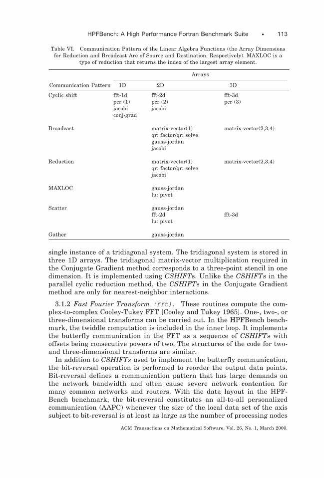
single instance of a tridiagonal system. The tridiagonal system is stored inthree 1D arrays. The tridiagonal matrix-vector multiplication required inthe Conjugate Gradient method corresponds to a three-point stencil in onedimension. It is implemented using CSHIFTs. Unlike the CSHIFTs in theparallel cyclic reduction method, the CSHIFTs in the Conjugate Gradientmethod are only for nearest-neighbor interactions.

3.1.2 Fast Fourier Transform (fft) . These routines compute the com-plex-to-complex Cooley-Tukey FFT [Cooley and Tukey 1965]. One-, two-, orthree-dimensional transforms can be carried out. In the HPFBench bench-mark, the twiddle computation is included in the inner loop. It implementsthe butterfly communication in the FFT as a sequence of CSHIFTs withoffsets being consecutive powers of two. The structures of the code for two-and three-dimensional transforms are similar.

In addition to CSHIFTs used to implement the butterfly communication,the bit-reversal operation is performed to reorder the output data points.Bit-reversal defines a communication pattern that has large demands onthe network bandwidth and often cause severe network contention formany common networks and routers. With the data layout in the HPF-Bench benchmark, the bit-reversal constitutes an all-to-all personalizedcommunication (AAPC) whenever the size of the local data set of the axissubject to bit-reversal is at least as large as the number of processing nodes

Table VI. Communication Pattern of the Linear Algebra Functions (the Array Dimensionsfor Reduction and Broadcast Are of Source and Destination, Respectively). MAXLOC is a

type of reduction that returns the index of the largest array element.

Communication Pattern

Arrays

1D 2D 3D

Cyclic shift fft-1d fft-2d fft-3dpcr (1) pcr (2) pcr (3)jacobi jacobiconj-grad

Broadcast matrix-vector(1) matrix-vector(2,3,4)qr: factor/qr: solvegauss-jordanjacobi

Reduction matrix-vector(1) matrix-vector(2,3,4)qr: factor/qr: solvejacobi

MAXLOC gauss-jordanlu: pivot

Scatter gauss-jordanfft-2d fft-3dlu: pivot

Gather gauss-jordan



along the axis subject to bit-reversal. A detailed analysis of the parallelFFT can be found in Johnsson et al. [1992].

The FFT is one of the most widely used algorithms in science, engineer-ing design, and in signal processing. Being a very efficient algorithm, FFThas relatively low operation count per data point, namely, O~logn!, but itscommunication is global and extensive. Hence, FFTs tend to expose weak-nesses in communication systems, in particular a low bisection bandwidth.It is also a good benchmark for the handling of complex arithmetic, and(local) memory hierarchies.

3.1.3 Gauss-Jordan Matrix Inversion (gauss-jordan) . Given a squarematrix A, the Gauss-Jordan routines compute the inverse matrix of A, A21,via the Gauss-Jordan elimination algorithm with partial pivoting [Goluband van Loan 1989; Wilkinson 1961]. Pivoting is required if the system isnot symmetric positive definite. The pivot element is chosen from the pivotrow, and the columns are permuted. At each pivoting iteration, this variantof the algorithm subtracts multiples of the pivot row from the rows aboveas well as below the pivot row. Thus, both the upper and lower triangular

Table VII. Computation-to-Communication Ratio and Memory Usage in the Linear AlgebraFunctions. In general, 1D, 2D, and 3D arrays are of size n, n2, and n3, respectively, exceptmatrix-vector and qr which use 2D arrays of size mn. matrix-vector , lu , qr , and pcroperate on multiple instances of matrices or linear systems, and the number of instances isdenoted using i. Finally, r denotes the number of right-hand sides of linear systems as in

lu , pcr , and qr .

FLOP Count Memory Usage CommunicationCode (per iteration) (in bytes) (per iteration)

conj-grad 26n 40n 4 CSHIFTs, 3 Reductions

fft-1d 5n 100n 2 CSHIFTsfft-2d 10n2 115n2 4 CSHIFTsfft-3d 15n3 136n3 6 CSHIFTs

gauss-jordan n~n 1 2 1 2n2! 32n2116n n Reduction, 3n Sends,2n Gets, 2n Broadcasts

jacobi n~6n2126n! 88n214n 2n CSHIFTs on 1D arrays,2n CSHIFTs on 2D arrays,2n Sends, 4n 1D to 2DBroadcasts

lu: nopivot 2 / 3n3i 8n~n 1 2r!i n Reduction, n Broadcastlu: pivot 2 / 3n3i 8n~n 1 2r!i n Reduction, n Broadcast

matrix-vector 2nmi 8~n 1 nm 1 m!i 1 Broadcast, 1 Reduction

pcr ~5r 1 12!ni 8~r 1 4!ni ~2r 1 4! CSHIFTs

qr: factor ~5.5m 2 0.5n!n2 36mn 2n Reductions, 2n Broadcastsqr: solve ~8m 2 1.5n!n2 44mn 1 8m~r 1 1! 2n Reductions, 4n Broadcasts

114 • Y. C. Hu et al.


matrices are brought to zero. An analysis of the numerical behavior of thealgorithm can be found in Dekker and Hoffman [1989]. Rather thanreplacing the original matrix with the identity matrix, this space is used toaccumulate the inverse solution.

Since there is no alignment between the layout of 1D arrays used astemporary arrays in swapping rows and columns of the 2D arrays duringtotal pivoting, data motion occurs in the swappings. SPREAD communica-tion is used for spreading pivot rows and columns to 2D temporary arrays.

3.1.4 Jacobi Eigenanalysis (jacobi) . The HPFBench routines are onlyvalid for real symmetric matrices. Given a real symmetric matrix A of sizen 3 n, the benchmark uses the Jacobi method to compute the eigenvaluesof the matrix A. Eigenvectors are not computed within the benchmark. TheJacobi method makes iterative sweeps through the matrix. In each sweep,successive rotations are applied to the matrix to zero out each off-diagonalelement. A sweep consists of the application of n~n 2 1! / 2 rotations. Aseach element is zeroed out, the elements previously zeroed out generallybecome nonzero again. However, with each step, the square root of the sumof the squares of the off-diagonal elements decreases, eventually approach-ing zero. Thus, the matrix approaches a diagonal matrix, and the diagonalelements approach the eigenvalues. For a detailed description of thismethod see Golub and van Loan [1989] and Schroff and Schreiber [1988].

The Jacobi eigenanalysis benchmark is interesting in that it uses both1D and 2D arrays with an extraction of the diagonal taking place incomputing rotation factors and an alignment and broadcast taking place inapplying the rotation factors. Aligning the 1D arrays with the 2D arrays

Table VIII. Characterization of the Application Kernels

Function HPFBench Code

Embarrassingly parallel gmo

Structured grid emulation 1D wave-1d2D boson, ellip-2d, step43D diff-3d, rp, mdcell4D qcd-kernel

Unstructured grid emulation fem-3d

Particle-particle interactionglobal 2D n-body

3D mdlocal 3D mdcell

Particle-grid interaction 2D pic-simple3D pic-gather-scatter, mdcell

FFT 1D wave-1d2D ks-spectral, pic-simple



result in poor load balance for the computation of rotation factors, while notaligning the arrays yields good load balance, but results in a potentiallyhigh communication cost.

The main communication patterns include nearest-neighbor CSHIFTsunder masks on 1D rotation vectors, SPREADs for duplicating 1D rotationvectors into 2D arrays, and CSHIFTs on 2D arrays.

3.1.5 LU Factorization (lu) . Given a dense square matrix A of size n3 n, and, a right-hand-side vector of size n, these routines solve the densesystem of equations AX 5 B by factoring the matrix A into a lowertriangular matrix L and an upper triangular matrix U, such that A 5LU. The factorization method is Gaussian elimination with or withoutpartial pivoting. Load balance is a well-known issue for LU factorization,and the desired array layout is cyclic distribution. Thus the lu benchmarkcodes uses two-dimensional arrays with cyclic distributions.

3.1.6 Matrix-Vector Multiplication (matrix-vector) . This HPFBenchbenchmark is a collection of routines computing one or more matrix-vectorproducts. Given arrays x, y, and A containing multiple instances [Johnssonet al. 1989] of the vectors x and y and the matrix A, respectively, thematrix-vector routines perform the operation y 4 y 1 Ax for each in-stance. The matrix-vector multiplication is implemented for the followingarray layouts:

Table IX. Data distributions of arrays in Dominating Computations of the ApplicationKernels, as Specified Using the DISTRIBUTE Directive. The distribution of an axis is eitherlocal to a processor, denoted as “*”, or sliced into uniform blocks and distributed across theprocessors, denoted as “b”, short for “block.” “Cyclic” distribution is not used in any of the

applications benchmarks.

Code

Arrays

Unstructured Grid1D 2D 3D 4D, 6D, 7D

boson X(*,b,b)diff-3d X(b,b,b)ellip-2d X(b,b)fem-3d X(*,b,b), X(*,*,b)gmo X(b) X(*,b)ks-spectral X(b,b)mdcell X(*,b,b,b)md X(b) X(b,b)n-body X(*,b)pic-simple X(*,b) X(*,b,b)pic-gather-scatter X(*,b) X(*,b,b)qcd-kernel X(*,b,b,b,b,b)

X(*,*,b,b,b,b,b)qmc X(b,b) X(*,*,b,b)qptransport X(b)rp X(b,b,b)step4 X(*,b,b)wave-1d X(b)

116 • Y. C. Hu et al.


(1) one instance of the three operands with each instance spread over allthe processors,

(2) multiple instances with each instance of each operand occupying asubset of the processors,

(3) multiple instances with each instance of the corresponding operandsallocated to the memory unit associated with one processor. This layoutrequires no communication and represents a truly embarrassinglyparallel case,

(4) multiple instances with the row axis (the axis crossing different rows)of array A allocated local to the processors, and the other axis of A aswell as the axes of the other operands spread across the processors.This layout only requires communication during the reduction.

For all cases, the spread-and-reduction algorithm is used, i.e., y 5sum~A p spread~x, dim 5 dim2!, dim 5 dim1!. Since a compiler typi-cally allocates some temporary arrays to store the intermediate resultswhen compiling the expression, the execution time for this implementationwill on most architectures be dominated by the SPREAD and SUM opera-tions, and the implicit alignments of the temporary arrays with inputarrays x and A and output array y.

Matrix-vector multiplication is a typical level-2 BLAS operation. It is thedominating operation in iterative methods for the solution of linear systemsof equations. It only requires two floating-point operations per matrixelement, and its performance is very sensitive to data motion. In case oneabove, each operand is distributed across all nodes such that the inputvector must be aligned with the matrix, and the result vector aligned withthe output vector as part of the computation.

3.1.7 Parallel Cyclic Reduction (pcr) . Parallel Cyclic Reduction is oneof the two tridiagonal solvers in HPFBench. It is different from the othertridiagonal solver, cond-grad , both in the systems to be solved and in themethods used. While cond-grad solves a single-instance tridiagonal sys-tem, this code handles multiple instances of the system AX 5 B. The threediagonals representing A have the same shape and are 2D arrays. One ofthe two dimensions is the problem axis of extent n, i.e., the axis alongwhich the system will be solved. The other dimension is the instance axis.For multiple right-hand sides, B is 3D. In this case, its first axis representsthe right-hand sides, is of extent r, and is local to a processor. Excludingthe first axis, B is of the same shape as each of the arrays for the diagonalA. The HPFBench code tests two situations, with the problem axis beingthe left and the right parallel axis, denoted as coef_inst and inst_coef ,respectively.

While cond-grad uses Conjugate Gradient method to solve tridiagonalsystems, the pcr benchmark solves the irreducible tridiagonal system oflinear equations AX 5 B using the parallel cyclic reduction method [Golub



and van Loan 1989; Hockney 1965; Hockney and Jesshope 1988], whichperforms the reduction and obtains the solution in one pass. Parallelimplementation issues are discussed in Johnsson [1985] and Johnsson andHo [1990]. The communication consists of circular shifts with offsets beingconsecutive powers of two and implemented by the intrinsic CSHIFT.

Like matrix-vector multiplication, few operations per data element areperformed. Each element in each solution vector is updated log n timesbefore its final value is available. However, only a few operations areperformed on an element after each CSHIFT communication, regardless ofn, and no replication or reduction is performed. Tridiagonal solvers exposecommunication overhead to a much greater extent than dense matrix-vector multiplication. In the latter case, the number of operations percommunicated element scales as O~ ÎM!, where M is the number ofelements of each submatrix residing on each processor [Johnsson et al.1989].

3.1.8 QR Factorization and Solution (qr) . This benchmark solvesdense linear systems of equations using Householder transformations[Dahlquist et al. 1974; Golub and van Loan 1989]. Given an m 3 ncoefficient matrix A, where m $ n, and a set of r right-hand-side vectors inthe form of an m 3 r matrix B, the QR routines factorize and solve thesystem of equations AX 5 B. The matrix A is factored into an orthogonalmatrix Q and an upper triangular matrix R, such that A 5 QR. Then, thesolver uses the factors Q and R to calculate the least squares solution tothe system AX 5 B, i.e., to compute the set of r vectors in array X (eachcorresponding to a particular right-hand side). The HPFBench version ofthe QR routines only supports single-instance computation and performsthe Householder transformations without column pivoting.

Both the factorization and the solution routines make use of masks. Analternative would be to use array sections. Whichever approach yields thehighest performance and requires the least memory depends upon how thecompiler handles masked operations, the penalty for carrying out opera-tions under masks, and how array sections are implemented, in particularwith respect to temporary storage.

The communication patterns appearing are SPREADs and reductions.The reductions are performed within the intrinsic function SUM. In thesolution routines, the right-hand-side matrix B is aligned with A throughassignment to another array (rhs ) of the same shape as A. Therefore, themisalignment overhead is reduced, at the expense of additional memoryspace. Due to this alignment, n $ r must hold. Thus the matrix sizes mustsatisfy the inequality m $ n $ r.

3.2 Application Kernels

The application kernel benchmarks are intended to cover computations(including communication) that dominate the running time of a wide

118 • Y. C. Hu et al.


variety of scientific applications frequently implemented on scalable archi-tectures. We characterize these benchmarks to assess their performanceaccording to some inherent properties that inevitably dictate their compu-tational structure and communication pattern.

Single-node performance is at least as important as the communicationrelated performance on most architectures. The HPFBench applicationkernels contain one “embarrassingly parallel” code, gmo, which does notinclude any interprocessor communication.

A large number of production codes are based on structured (regular)discretizations of space or time. Many solution methods imply data refer-ences along the axes of grids resulting from such discretizations. Formethods of relatively low order with respect to accuracy, the data refer-ences associated with updating variables at grid points are confined toneighborhoods that extends one or two grid points in all directions. Forcomputations of this nature, the efficient support of communication asdefined by the grid is often crucial. The HPFBench application kernelscontain codes that depend on the emulation of grids distributed acrossprocessors as follows: one-dimensional grids: wave-1d ; two-dimensionalgrids: boson , ellip-2d , and step4 ; three-dimensional grids: diff-3d , rp ,and mdcell ; four-dimensional grids: qcd-kernel .

Since the geometries involved are often complex, unstructured (irregular)grids are the most common form of spatial discretizations in engineeringapplications, and the finite-element method is a common solution tech-nique. The collection of elements is typically represented as a list ofelements with arrays describing the connectivity or adjacency. The fem-3dHPFBench benchmark is intended to cover some of the aspects of this typeof codes. This benchmark uses an iterative solver for the equilibriumequations. The execution time is dominated by matrix-vector multiplica-tion, which is in turn dominated by gather and scatter operations on theunstructured grid (unassembled stiffness matrix).

In addition to codes solving field problems for a variety of domain shapesand media, many computations also involve discrete entities, like particles.The so-called N-body codes solve field equations based on particle-particleinteractions with or without spatial discretizations. Traditional N-bodycodes do not use a spatial discretizations and have an arithmetic complex-ity of O~N 2!. The so-called particle-in-cell (pic) codes make explicit use of agrid for long-range interaction and require the representation of bothparticle attributes and grid-point data. Hierarchical N-body codes of arith-metic complexity O~N log N ! or O~N ! construct a hierarchy of grids.

The HPFBench benchmark suite contains two codes that carry out directinteraction between all particles: md for particle interaction in three-dimensional space, and n-body for particle interaction in two-dimensionalspace.

The HPFBench codes involving both grid and particle representations arepic-gather-scatter and mdcell (with three-dimensional grids) as wellas pic-simple (with a two-dimensional grid).



A particularly important computational kernel is the FFT, for whichefficient implementations appear in many libraries. The HPFBench suiteincludes three application kernels that make extensive use of the FFT:ks-spectral and pic-simple perform FFTs on two-dimensional grids,while wave-1d performs FFTs on a one-dimensional grid.

Several benchmarks (pic-simple , qmc, qptransport , and wave-1d )rely on a random-number generator for problem initialization. AlthoughFortran 90 provides an intrinsic function (RANDOM NUMBER) for ran-dom-number generation, the sequence the intrinsic function generatesseems to vary with different F90 compilers. To ensure the same problem issolved for these benchmarks under different HPF compilers and on differ-ent platforms, we provide our random-number generator wrapper as anHPFBench utility function. The wrapper calls the UNIX C library functiondrand48() which is both compiler- and architecture-independent. Oneconsequence of this change is that initializing a distributed array will beserialized. Since a random-number generator is only called during initial-ization, we consider this serialization to be acceptable.

The above characterization of the application kernels is summarized inTable VIII. Table IX lists the data representation and layout for the arraysused in the dominating computations in the application kernels, and TableX summarizes the communication patterns in the codes. Table XI tabulatesthe implementation techniques for the stencil, gather/scatter, and AABCcommunication patterns, whereas Table XII lists the computation-to-com-munication ratio for the main loop of application codes, as well as thememory usage.

3.2.1 Boson: Many-Body Simulation (boson) . This benchmark per-forms quantum many-body computations for bosons on a two-dimensionallattice using a grid-based Monte Carlo technique. The code uses a Carte-sian lattice with periodic boundary conditions and uniform site connectivityresulting in stencil communication. The algorithms are outlined and dem-onstrated in Batrouni and Scalettar [1992], Hirsch et al. [1982], andTobochnik et al. [1992].

The implementation uses 3D arrays, with the first axis representing thetime axes, and the other two axes representing the two spatial axes of thegrid. Nearest-neighbor CSHIFTs are heavily used along the spatial axes.The CSHIFTs are interleaved with computations in a way that precludesthe use of a linear stencil formulation as well as the use of polyshift(PSHIFT [George et al. 1994]). The main computations are scalar opera-tions among 2D parallel arrays, i.e., the 3D arrays with the time axeslocally (and sequentially) indexed.

3.2.2 3D Diffusion Equation: Explicit Finite Difference (diff-3d) .This diffusion equation simulation is the integration of the three-dimen-sional heat equation using an explicit finite difference algorithm, which isstable subject to the Courant condition dt , dx2 / D, where D is thediffusivity. The benchmark code fully exploits the fact that the stencil

120 • Y. C. Hu et al.


coefficients are the same for all grid points (constant coefficients). Thusneither left-hand-side nor right-hand-side matrices are stored explicitly in

Table X. Communication Patterns in the Application Kernels

CommunicationPattern

Arrays

1D 2D 3D (4,5,6,7)-D

Stencil wave-1d ellip-2d rp, diff-3d

step4

Gather pic-simple fem-3dpic-gather-scatter

Scatter qptransport pic-gather-scatter mdcell

Scatterw/combine

qmc fem-3d

pic-gather-scatter

Reduction qptransport ellip-2dks-spectralmdqmcrp

Broadcast ellip-2d,md qmcn-body,rp

AABC md, n-body

Butterfly (FFT) wave-1d pic-simpleks-spectral

Scan qptransport qmc pic-gather-scatter

Cyclic shift wave-1d ellip-2d boson mdcelln-body rp qcd-kernelstep4

Sort pic-gather-scatterqptransport



this benchmark. Only the solution variables F~x, y, z, t! are stored inarray form for one time step as a 3D array of shape nx 3 ny 3 nz.

The operations in this benchmark are dominated by the evaluation of aseven-point centered difference stencil in three dimensions. The communi-cation is implemented by array sections. Instead of array sections,CSHIFTs could have been used. This implementation technique is used inellip-2d , which evaluates five-point stencils in two dimensions, and therp benchmark which also performs a seven-point centered stencil in threedimensions, just as diff-3d . Stencil evaluations are interesting from acompiler evaluation perspective because they occur frequently in a varietyof application codes, and there are many opportunities for optimization ofdata motion between processing elements, and between memory and regis-ters. Some of these issues, related to the data-parallel programmingparadigm, are explored in Hu and Johnsson [1996], while some compilertechniques are explored in Brickner et al. [1993].

This benchmark is an example of applications with structured Cartesiangrids, solving homogeneous linear differential equations with constantboundary conditions.

3.2.3 Solution of Poisson’s Equation by the Conjugate Gradient Method(ellip-2d) . This benchmark uses the preconditioned Conjugate Gradi-ent method to solve Poisson’s equation on a regular two-dimensional grid

Table XI. F90/HPF Constructs Used in Implementing Some Common CommunicationPatterns in the Application Kernels

CommunicationPattern Code Implementation Techniques

Stencil boson CSHIFTellip-2d CSHIFTmdcell CSHIFTrp CSHIFTwave-1d CHSIFTstep4 chained CSHIFTsdiff-3d Array sections

Gather fem-3d FORALL with indirect addressingpic-gather-scatter FORALL with indirect addressingpic-simple FORALL with indirect addressing

Scatter mdcell INDEPENDENT DO w/indirect addressingpic-gather-scatter FORALL with indirect addressingqptransport indirect addressing

Scatter w/combine fem-3d HPF sum_scatter library procedurepic-gather-scatter HPF sum_scatter library procedureqmc HPF copy_scatter library procedure

AABC md SPREADn-body CSHIFT, SPREAD, scalar to array assignment

122 • Y. C. Hu et al.


with Dirichlet boundary conditions. The Poisson’s equation is discretizedwith a centered five-point stencil. The matrix-vector product in the Conju-gate Gradient algorithm [Dahlquist et al. 1974; Golub and van Loan 1989;Press et al. 1992] takes the form of a stencil evaluation on the two-dimensional grid. In addition, one reduction and one broadcast is requiredfor the Conjugate Gradient method.

Compared to diff-3d , this HPFBench benchmark is dominated by theevaluation of a two-dimensional stencil instead of a three-dimensionalstencil. Hence, for a given subgrid size, the optimum computation-to-communication ratio (volume/surface) is higher for ellip-2d . However,the inner products and broadcast require some communication, but it can

Table XII. Computation-to-Communication Ratio and Memory Usage in Main Loop ofApplication Kernels. In applications involving structured grids, nx, ny, nz denote the number

of mesh points along x-, y-, and z-axes. In particle simulation applications, np denotes thenumber of particles. nt denotes the extent of time axis in quantum dynamics applicationsboson and qcd . In fem-3d , nve and ne denote the number of vertices per element and the

number of elements in an unstructured mesh. Problem sizes in gmo and qmc are moreinvolved and are detailed in the code.

CodeFLOP Count Memory Usage Communication

(per iteration) (in bytes) (per iteration)

boson 4~258 1 36 / nt! z

ntnxny

40nxny 1 128nt 112000 1 4000mb

1 1536ntnxny

38 CSHIFTs

diff-3d 9~nx 2 2! z 8nxnynz 1 7-point Stencil~ny 2 2!~nz 2 2!

ellip-2d 38nxny 96nxny 4 CSHIFTs, 3 Reductions

fem-3d 18nvene 56nvene 1 140nv

11200ne

1 Gather, 1 Scatter w/combine

gmo 6000nvec 2nvec z ~8 z nsout z N/A~ntrout11! 18 1 8 z nvec)

ks-spectral ~76 1 40log2nx! z 144nxny 8 1D FFTs on 2D arraysnxny

mdcell ~101 1 392np! z ~184 1 160np! z 195 CSHIFTs,npnxnynz nxnynz 7 Scatters on local axis

md ~23 1 51np!np 160np 1 80np2 6 1D to 2D SPREADs,

3 1D to 2D sends,3 2D to 1D Reductions

n-bodyBroadcast 17np

2 72np 3 BroadcastsSPREAD 17np

2 72np 3 SPREADs, 3 SPREADsCSHIFT 17np~np 2 1! 72np 3 CSHIFTs, 3 CSHIFTsCSHIFT-sym. 13.5np~np 2 1! 96np 3 CSHIFTs



be made very efficient. The three dominating operations with respect toperformance on many scalable architectures in this benchmark are thereduction (SUM), broadcast, and the evaluation of the five-point centereddifference stencil.

This benchmark is an example of a class of applications with structuredgrids, involving the solution of linear nonhomogeneous differential equa-tions with Dirichlet boundary conditions by means of an iterative solver.From a performance point of view, like diff-3d , this benchmark isinteresting, since it discloses how efficiently stencil communication andevaluation are handled by the compiler.

3.2.4 Finite-Element Method in Three Dimensions (fem-3d) . Thisbenchmark uses the finite-element method on trilinear brick elements tosolve the equilibrium equations in three dimensions. The mesh is repre-sented as an unstructured mesh. Specifically, this code evaluates theelemental stiffness matrices and computes the displacements and thestresses at the quadrature points using the Conjugate Gradient method onunassembled stiffness matrices [Johnson 1987; Johnson and Szepessy1987].

Table XII. Continued

CodeFLOP Count Memory Usage Communication

(per iteration) (in bytes) (per iteration)

pic-simple np 1 15nxny z 64np 1 72nxny 1 Scatter w/ add 1D to 2D,~lognx 1 logny! 3 FFT, 1 Gather 3D to 2D

pic-gather-scatter

270 np 12nxnynz 1 88np 81 Scans, 27 Scatters w/add,27 1D to 3D Scatters,27 3D to 1D Gather

qcd-kernel 606nxnynznt 720nxnynznti 4 CSHIFTs

qmc @~42 1 2nonmaxw! z

npndnwne 1~142no 1 251! z

nwne#nb

16npnd 1 96nwne nmaxw SPREADs 3D to 1D,5 Reductions 2D to 1D,~npnd 1 4! Scans on 2D,~npnd 1 1! Sends,3 Reductions 2D to scalar

qptransport 34n 160n 10 Scatters 1D to 1D,1 Sort, 5 Scans, 1 CSHIFT,1 EOSHIFT, 3 Reductions

rp 44nxnynz 120nxnynz 2 Reductions, 12 CSHIFTs(2 7-point Stencils)

step4 2500nxny 1000nxny 128 CSHIFTs(8 16-point Stencils)

wave-1d 29nx 1 10nxlognx 64nx 12 CSHIFTs, 2 1D FFTs

124 • Y. C. Hu et al.


The unstructured mesh is read from a file and stored in the elementnodes array. A partitioning of the unstructured mesh is performed in anattempt to minimize the surface area (communication) for the collection ofelements stored in the memory of a processor. The partitioning is carriedout by Morton ordering (implemented in HPF as a general partitioningmethod in Hu et al. [1997]) of the elements using the coordinates of theelement centers. The array of pointers derived from the unstructured meshis reordered so that the communication required by the subsequent gatherand scatter operations is reduced. The nodes are also reordered via Mortonordering. The nodes of the mesh are stored in a 2D array whose first axis islocal to a processing element. It represents the coordinates of each node.The computations of the benchmark are dominated by the sparse matrix-vector multiplication required for the Conjugate Gradient method. It isperformed in three steps: a gather, a local elementwise dense matrix-vectormultiplication, and a scatter. The elementwise matrix-vector multiplicationexploits the fact that the elemental stiffness matrices are symmetric.

The fem-3d is a good example of finite-element computations on unstruc-tured grids. In order to preserve locality of reference and allow for blocking,and the use of dense matrix optimization techniques, finite-element codesare often based on unassembled stiffness matrices. Moreover, by exploitingsymmetry in the elemental stiffness matrices, this code is a good test casefor compiler optimizations with respect to local memory references for asomewhat more complex situation than a dense nonsymmetric matrix.Through the use of the reordering of the mesh points and nodes to improvelocality, the gather and scatter operations are expected to be efficient.

3.2.5 Seismic Processing (gmo) . This benchmark is a highly optimizedHPF code for a generalized moveout seismic kernel for all forms of Kirchhoffmigration and Kirchhoff DMO (also known as x 2 t migration and x 2 tDMO). For each vector unit, the code explicitly strip-mines the maincomputational loop into vector chunks of length nvec. In order to performthe strip-mining, the indices isamp , ksamp, and the real variable del havea local axis of extent equal to the vector length nvec. independent doloops are used to express each calculation in the loop for one whole vectorchunk and across all the vector units. An outer do-loop steps through allthe vector chunks sequentially.

The gmo benchmark is a good test case of a compiler’s local memorymanagement. The code is written explicitly with efficient local memorymanagement in mind.

3.2.6 Spectral Method: Integration of Kuramoto-Sivashiniski Equations(ks-spectral) . This benchmark uses a spectral method to integrate theKuramoto-Sivashiniski equations on a two-dimensional regular grid. Thetwo-dimensional grid is stored in a two-dimensional array with blockdistribution. The code performs the integration using a fourth-order Runga-Kutta integration of the equation dX / dt 5 f~ X, t! with step size dt.Within an integration step, the core computation is a 2D FFT performed on



the grids. In fact, all the communication in the benchmark happens insidethe 2D FFT.

3.2.7 Molecular Dynamics, Lennard-Jones Force Law (md, mdcell) .Many molecular dynamics codes make use of the Lennard-Jones force lawfor particle interaction. With few exceptions, this force law is applied with acut-off radius. A grid is superimposed on the domain of particles, and thecell size of the grid is chosen such that the cut-off radius is smaller than thecell size. This guarantees that interaction only involves particles in adja-cent cells. Furthermore, if the cell size is only moderately larger than thecut-off radius, then, for simplicity in implementation, all particles inadjacent cells are assumed to interact, and no separate interaction lists aremaintained. The loss of efficiency is modest. The HPFBench mdcell code isdesigned with these assumptions. Accurate modeling of electrostatic forcesdoes, however, require long-range interaction between particles, in whichcase the radius cannot be cut off. Thus, molecular dynamics codes thatattempt to include electrostatic forces must evaluate interactions betweenall particles, i.e., such codes have many aspects in common with generalN-body codes. The HPFBench code md carries out an evaluation of interac-tions between all particles using a Lennard-Jones potential without cut-off.The mdcell and the md codes both use a Maxwell initial distribution and aVerlet integration scheme. Both benchmarks make heavy use of parallelindirection.

—Local forces only: In the mdcell code particles only interact with parti-cles in nearby cells; thus no neighbor tables are required. The benchmarkassumes periodic boundary conditions and initializes particles with theMaxwell distribution.The particles are initialized and manipulated in 4D arrays, i.e., the firstaxis is local and is used for storing particles in the same cell, while theother axes are parallel, representing the 3D grid of cells. Utilizing thesymmetry, each cell only needs to fetch directly 13 neighbor cells insteadof all 26 in the neighbor-cell interaction. The fetching of neighbor cells isperformed via CSHIFT. No linear ordering [Lomdahl et al. 1993] isimposed on the order of fetching the 13 neighbors; therefore the numberof CSHIFTs is not minimized. The migration of particles are imple-mented by slicing through the 4D particle arrays and copying particlesthat need to move to different cells out to a newly allocated slice of the4D array, followed by a scatter operation within the local axis of the 4Darray to squeeze out the “bubbles” in the array. Since particle can at mostmove to a neighboring cell, the copying operation is implemented using aCSHIFT.

—Long-range forces: The md code carries out a Lennard-Jones force lawwithout cut-off. The interaction is evaluated directly through an O~N 2!method. The all-to-all communication is implemented with a send-spread-reduce algorithm. Each particle attribute is implemented as a 1Darray. For instance, particle positions are implemented as three 1D

126 • Y. C. Hu et al.


arrays with a location for each particle. The all-to-all communicationmakes use of 2D temporary n 3 n arrays, where n is the number ofparticles. The particle information is spread across both dimensionsusing SPREAD operations.

3.2.8 A Generic Direct N-Body Solver, Long-Range Forces (N-Body) .This benchmark consists of a suite of two-dimensional N-body solvers all ofwhich directly compute all pairwise interactions [Hockney and Eastwood1988]. The different codes in the suite allows for a comparison of differentways of programming the all-to-all communication. The different ways ofprogramming the direct method are described in detail with code listings inGreenberg et al. [1992]. The data structures consist of 2D arrays with thefirst dimension local to a node, holding the particle information, and thesecond parallel, representing the number of particles. The all-to-all commu-nication for the direct method is implemented with four different commu-nication patterns:

(1) Broadcast, implemented as an assignment of a single array element toan array,

(2) SPREAD, implemented using SPREAD,

(3) CSHIFT, implemented using CSHIFT,

(4) CSHIFT, implemented using CSHIFT, and exploiting symmetry.

3.2.9 Particle-in-Cell Codes (pic-simple, pic-gather-scatter) .The HPFBench benchmark suite contains two codes for particle-in-cellmethods. Both codes represent a structured grid in the form of 3D arrays,but differ in their representation of particle attributes. The pic-simplecode implements a two-dimensional spatial grid with a third local axis forvector values at the grid points and a 2D array for particles, with theattributes for each particle forming a local axis. The pic-gather-scattercode implements a three-dimensional spatial grid for a scalar field, whileeach particle attribute is represented by its own 1D array.

The long-range particle interaction in particle-in-cell codes is determinedby solving field equations on the grid by some efficient method, like theFFT, interpolating the field to particles in a cell, moving the particles, andthen projecting back to the grid points. The pic-simple code scatters fielddata from the particles to the grid with send-with-add, whereas thepic-gather-scatter code accomplishes this task with both send-with-add and sort-scan-with-add.

—Straightforward implementation: The pic-simple benchmark repre-sents a two-dimensional electrostatic plasma simulation. It is meant tobe a naive implementation of the method, representative of the sort ofparallel code that users would write on their first attempt.The particle information is represented by 2D arrays, with the first axisbeing local to a processing element and storing the relevant attributes foreach particle. Initially, the particles are placed randomly according to a



uniform distribution inside a square box of shape cr 3 cr. This box iscentered in the domain. Each particle is given a random velocity in therange @2cv / 2, cv / 2# along the x- and y-axes, which is modified with acomponent normal to, and proportional to, the vector from the box centerto the particle. The magnitude of this modification vector is cl. Thetwo-dimensional grids are represented by 3D arrays, again with the firstaxis being local and representing the 2D vector field at each gridpoint.The computations consist of scattering the charge data from the particlesto the grid points using sum_scatter. Charge data sent to the samegridpoint are combined on-the-fly, and no sophisticated interpolationscheme is used. Then, a two-dimensional FFT is used to solve Poisson’sequation for the electrostatic field on the two-dimensional grid. This isfollowed by invoking a gather operation to determine the field at theparticles. Then, the particle positions and velocities are advanced intime, using a leap-frog method.

—Sophisticated implementation: The pic-gather-scatter benchmarktests the gather/scatter operations between data structures for particlesand for cells in a typical 3D particle-in-cell application. The solver for thefield equations on the grid is not included. Two different techniques forparticle-grid interactions are used: send-with-add and sort-scan-send.The sort-scan-send version avoids congestion, which occurs in the send-with-add version. The sort-scan-send version also uses a more sophisti-cated interpolation function in distributing the charges (masses, etc.) tothe grid.The particle positions are stored in a 2D array, with the first axis beinglocal and representing the three coordinates of a particle position. Thefield at the grid points is stored in 3D arrays, the first axis of which islocal while the other two are parallel. Hence, this layout does notminimize the surface to volume ratio.The benchmark makes extensive use of HPF library code for manycommunication and the sorting functions, including sum_scatter, sum_prefix, copy_ prefix, and grade_up.The scan-and-send sorts particles into canonical ordering using theconcatenated coordinates of a particle, i.e., ~z?y?x!, as its key. Thisordering differs from the ordering of the cells and gridpoints in that theaddress space for the cells and grid points is three-dimensional. Using acoordinate-sort for the particles as described in Hu and Johnsson [1996]should improve the locality in the send and get operations between the1D particle arrays the 3D grid arrays.

3.2.10 QCD Kernel: Staggered Fermion Conjugate Gradient Method(qcd-kernel) . This benchmark represents the kernel of a staggeredfermion Conjugate Gradient algorithm for Quantum Chromo-Dynamics(QCD). The operation performed is

128 • Y. C. Hu et al.


r~x! 5 mc 1 Om51

4

@u~x!†c~x 1 m! 2 u~x 2 m!c~x 2 m!#

where all the entities are double complex, except m which is a doubleconstant. r and c represent three-element “vectors” (the three colors), and urepresents a 3 3 3 operator between colors; † denotes the adjoint operator.The aforementioned operation is carried out on a four-dimensional lattice ofshape nx 3 ny 3 nz 3 nt (three spatial and one time dimension). Theinteger m loops over the four dimensions of the lattice, so x 6m is aneighboring lattice point along dimension m. This method is described indetail in Aoki et al. [1991], which is also an excellent source of bibliographyon the subject.

The qcd-kernel benchmark is implemented as a multiple-instance code,with 5D arrays for lattice data, or more for nonscalar fields. The kernel ishighly optimized in the following ways:

—All the complex entities are declared as a pair of real values (real andimaginary parts separately) to avoid operations on complex data types(and relying on the compiler to translate them).

—The 3 3 3 operator u is represented as a vector of length nine, so thatboth u and its transpose can be accessed without any extra space ormapping overheads.

—Matrix operations are calculated element by element by straight-linecode; the only loop overhead is the sequential loop for m over the fourdimensions.

—Only the five dimensions for the multiple-instance lattice (four dimen-sions for space and time and one dimension for the nins instances) areparallel; other dimensions are local. Thus, the only communication is thecircular shifts x 6m.

The qcd-kernel benchmark is interesting as an example of how efficientlocal arithmetic can be carried out on small matrices, and it is a goodreference for compiler optimizations local to a node.

3.2.11 Quantum Monte-Carlo (qmc) . This benchmark evaluates theground-state energy for two fermions confined in a one-dimensional squarepotential well using a Green’s function quantum Monte Carlo method. Thebasic algorithm consists of moving random walkers in configuration space(two-dimensional in this model problem) by sampling their steps from theGreen’s function for the Helmholtz equation, and multiplying their weightsby a factor that is a function of configuration space position. For a thoroughdescription of the algorithmic methodology see Anderson et al. [1991].

To load balance the calculation high-weight particles are split, andlow-weight particles are killed at each step. This kill-and-split algorithm is



implemented with scans and sends and is described in Traynor et al.[1991].

The manifestation of the fermion sign problem in this calculation is thetendency of large numbers of walkers of opposite sign to collect in the sameregion of configuration space. To mitigate this problem, a walker-cancella-tion scheme is used, as described in Anderson et al. [1991]. This amounts toan N-body problem on the walkers, and it is implemented using thesequential spread algorithm every nc (cancellation number) iteration steps.Thus, by making nc large, this code is a good test of the scan-and-sendload-balancing algorithm. By making nc small, it is a good test of thesequential SPREAD N-body algorithm. Both limits are examined in thistest suite.

The main data structures of the code are 4D arrays, with the first twoaxes being local to a node and representing a walker, and the other twoaxes being parallel, representing the independent ensembles of walkers.Most computations, however, are performed on 2D arrays corresponding tothe two parallel axes of the 4D arrays. The communication includesreductions along one axis of these 2D arrays, scatter with combine on 2Darrays implemented via copy_scatter, and scan operations by calling theHOF intrinsic functions copy_ prefix and sum_ prefix along one dimension ofthe 2D arrays.

3.2.12 Quadratic Programming Problem (qptransport) . This bench-mark is an optimization code for finding optimum paths on a bipartitegraph with a quadratic cost function. The benchmark generates randomsparse quadratic transportation problems and solves them using an un-usual alternating direction method. Each problem is based on a large,sparse, bipartite graph. The graph vertices are either “sources” (with anexogenous supply of some commodity) or “sinks” (with a demand). Theedges of the graph connect the sources and sinks, and each one has aquadratic cost function. The problem is to route the commodity from thesource nodes to the sink nodes so as to exactly use all of the supplies andsatisfy all demands with the minimum possible total cost. The examplecode generates problems, solves them, and checks that the solutions seemapproximately correct. However only the solution phase is timed. It repre-sents the graph as one long vector with many short segments of averagelength 16.

The code performs very few FLOPs and is dominated by many rank, scan,and scatter operations on 1D arrays by calling the HPF library functions,grade_up, sum_ prefix, min_ prefix, copy_ prefix, and indirect addressing. Itis believed that rank and scan operations that could recognize and takeadvantage of all the short segments being short would substantially speedup this benchmark.

3.2.13 Solution of Nonsymmetric Linear Equations Using the ConjugateGradient Method (rp) . This benchmark solves a nonsymmetric linearsystem of equations that result from seven-point centered difference ap-proximations of the differential operators in the following equation:

130 • Y. C. Hu et al.


d2u

dx21

d2u

dy21

d2u

dz21 d~x!

du

dx1100.0

du

dy1100.0

du

dz5 F

where d~x! is a polynomial function of x. F is never explicity specified.Instead, a solution vector u is set up as a vector of all ones, and then theright-hand-side vector is derived from the linear system of equations. ThePDE assumes Dirichlet boundary condition, and the domain is descretizedby a regular grid in three dimensions. The particular method employeduses the single-node version of Conjugate Gradient accelerated Cimminorow projections [Bramley and Sameh 1992; Cimino 1939]. That is, theConjugate Gradient method is applied to the normal equations ATAx 5ATb, where A is a nonsymmetric matrix with seven diagonals. Eachunknown in the equation corresponds to a gridpoint in the three-dimen-sional grid, and the matrix A is represented in seven 3D arrays.

The multiplication ATAx is implemented as two matrix-vector multiplica-tions, i.e., AT~Ax!. Since the matrix A is represented in seven 3D arrays,each matrix-vector multiplication becomes a seven-point stencil evaluation.The stencil is implemented using CSHIFTs, which involve movement ofdata interior to the subgrid on each processor, as well as actual interpro-cessor communication of data on the boundary of each subgrid. The localdata movement can be eliminated via restructuring the code using thearray aliasing feature of CMF [Hu and Johnsson 1999].

This code is dominated by two seven-point centered stencils in threedimensions, global reduction, and broadcast. One of the two stencil evalua-tions has variable coefficients with a single-source array, while the otherstencil evaluation has a different source array for each shift. Stencils withmultiple sources are common in the solution of Navier-Stokes equations.

3.2.14 Explicit Finite Difference in Two Dimensions (step4) . Thisbenchmark solves a subsonic Euler flow over a backward-facing step. Themethod employed uses fourth-order accurate finite difference equations.Artificial viscosity is used to stabilize the numerical method.

The communication pattern for the difference operations involves a16-point stencil with four stencil points coming from each direction: north,east, south, and west, as shown in Table X. The 16-point stencil isimplemented as four four-point stencils, one along each axis. Each four-point stencil is in turn implemented using chained CSHIFTs. For boundarypoints, some stencil points are truncated at the boundary, and fewer stencilpoints are employed. As a consequence, a combination of third-orderaccurate (for boundary points) and sixth-order accurate (for interior points)local approximations is used which guarantees fourth-order global conver-gence [Olsson 1994; 1995a; 1995b].

3.2.15 Wave Equation (wave-1d) . This benchmark simulates the inho-mogeneous one-dimensional wave equation using the method of character-istics. It does a spline fit to the function at every time step and makes



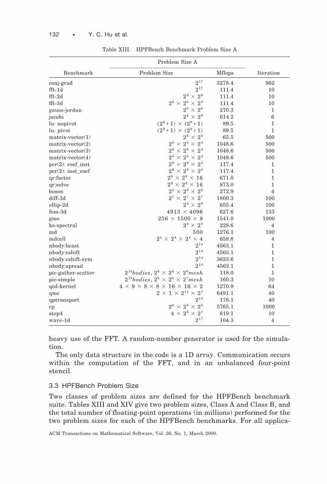
heavy use of the FFT. A random-number generator is used for the simula-tion.

The only data structure in the code is a 1D array. Communication occurswithin the computation of the FFT, and in an unbalanced four-pointstencil.

3.3 HPFBench Problem Size

Two classes of problem sizes are defined for the HPFBench benchmarksuite. Tables XIII and XIV give two problem sizes, Class A and Class B, andthe total number of floating-point operations (in millions) performed for thetwo problem sizes for each of the HPFBench benchmarks. For all applica-

Table XIII. HPFBench Benchmark Problem Size A

Problem Size A

Benchmark Problem Size Mflops Iteration

conj-grad 217 3278.4 962fft-1d 217 111.4 10fft-2d 29 3 28 111.4 10fft-3d 26 3 26 3 25 111.4 10gauss-jordan 29 3 29 270.3 1jacobi 28 3 28 614.2 6lu: nopivot ~2911! 3 ~2911! 89.5 1lu: pivot ~2911! 3 ~2911! 89.5 1matrix-vector(1) 28 3 28 65.5 500matrix-vector(2) 28 3 28 3 24 1048.6 500matrix-vector(3) 28 3 28 3 24 1048.6 500matrix-vector(4) 28 3 28 3 24 1048.6 500pcr(2): coef_inst 29 3 29 3 23 117.4 1pcr(2): inst_coef 29 3 29 3 23 117.4 1qr:factor 29 3 29 3 16 671.0 1qr:solve 29 3 29 3 16 873.0 1boson 25 3 26 3 26 272.9 4diff-3d 27 3 27 3 27 1800.3 100ellip-2d 29 3 29 655.4 100fem-3d 4913 3 4096 627.6 133gmo 256 3 1500 3 8 1541.0 1000ks-spectral 29 3 28 228.6 4md 500 1276.1 100mdcell 24 3 24 3 24 3 4 658.8 4nbody:bcast 214 4563.1 1nbody:cshift 214 4563.1 1nbody:cshift-sym 214 3623.6 1nbody:spread 214 4563.1 1pic-gather-scatter 218bodies, 26 3 26 3 26mesh 118.0 1pic-simple 218bodies, 26 3 26 3 27mesh 160.3 10qcd-kernel 4 3 9 3 8 3 8 3 16 3 16 3 2 1270.9 64qmc 2 3 1 3 211 3 27 6491.1 40qptransport 213 178.1 40rp 26 3 26 3 25 5765.1 1000step4 4 3 28 3 27 819.1 10wave-1d 217 104.3 4

132 • Y. C. Hu et al.


tions, the problem sizes are chosen so that the total memory requirementwould be around 50MB for Class A and 200MB for Class B. Therefore, theClass B problem sizes approach the capacity of the main memory in asingle processor of most modern distributed-memory machines. Largerproblem sizes will be added in the future when there is a significantincrease of the main memory in the processors of parallel machines. Formost mesh-based codes, the 200MB total memory requirement of Class Btranslates into about 220 mesh points, i.e., 210 3 210 in 2D or 27 3 27 3

26 in 3D. For Class A, the 50MB requirement translates into about 217

mesh points.

Table XIV. HPFBench Benchmarks Problem Size B

Problem Size B

Benchmark Problem Size Mflops Iteration

conj-grad 220 26227.2 962fft-1d 220 1048.6 10fft-2d 210 3 210 1048.6 10fft-3d 27 3 27 3 26 1048.6 10gauss-jordan 210 3 210 2148.5 1jacobi 29 3 29 4872.7 6lu: nopivot ~21011! 3 ~21011! 717.9 1lu: pivot ~21011! 3 ~21011! 717.9 1matrix-vector(1) 210 3 210 1048.6 500matrix-vector(2) 210 3 210 3 24 8388.6 500matrix-vector(3) 210 3 210 3 24 8388.6 500matrix-vector(4) 210 3 210 3 24 8388.6 500pcr(2): coef_inst 210 3 210 3 23 521.1 1pcr(2): inst_coef 210 3 210 3 23 521.1 1qr:factor 210 3 210 3 16 5369.0 1qr:solve 210 3 210 3 16 6979.0 1boson 25 3 27 3 27 2173.7 4diff-3d 28 3 28 3 28 14402.4 100ellip-2d 210 3 210 2621.4 100fem-3d 4913 3 4096 627.57 133gmo 1024 3 1500 3 8 6162.0 1000ks-spectral 210 3 29 998.2 4md 1372 9603.2 100mdcell 25 3 25 3 25 3 4 5270.4 4nbody:bcast 215 18253.6 1nbody:cshift 215 18253.6 1nbody:cshift-sym 215 14495.1 1nbody:spread 215 18253.6 1pic-gather-scatter 220bodies, 27 3 27 3 27mesh 471.9 1pic-simple 220bodies, 27 3 27 3 27mesh 718.2 10qcd-kernel 4 3 9 3 16 3 16 3 16 3 16 3 2 1270.8 64qmc 2 3 1 3 213 3 27 25963.0 40qptransport 216 1426.1 40rp 27 3 27 3 27 46140.0 1000step4 4 3 210 3 29 13107.0 10wave-1d 220 960.5 4



3.4 Core HPFBench Benchmarks

The large number of benchmarks included in the HPFBench suite strive tocover a wide variety of computational structures and communication pat-terns found in differnet disciplines. Nevertheless, it can be too strenuousfor vendors to evaluate an HPF compiler using the full set of benchmarks.Therefore, we pick a subset of eight benchmarks to form the core HPF-Bench Suite. The criteria in picking the core benchmarks are to cover asmany F90/HPF constructs, array distributions, computational structures,communication patterns, and different implementations of them as possi-ble. The core suite consists of two from the linear algebra subset—fft andlu —and six from application kernels—ellip-2d , fem-3d , mdcell , pic-simple , pic-gather-scatter , and rp .

4. EVALUATION RESULTS OF PGHPF ON THE IBM SP2

We report on the results of evaluating an industry-leading HPF compiler,pghpf , from the Portland Groups, Inc., on the distributed-memory IBMSP2, using all 25 benchmarks in the HPFBench suite. Version 2.2-2 ofpghpf with compiler switch -O3 -W0,-O4 was used and linked with -Mmpl .To measure the overhead of HPF compilers on a single node, we alsomeasure the performance of the HPF versions of the codes compiled underpgf90 with the same compiler switchs as above plus -Mf90 and linked with-rpm1, and the performance of the sequential code compiled using thenative Fortran 77 compiler, xlf, with compiler flag -O4 .

Our evaluation was performed on an IBM SP2 with 16 uniprocessornodes. Each node has a RS6000 POWER2 Super Chip processor runningAIX 4.3 at 120MHz and has 128MB of main memory. The nodes arecommunicating through IBM’s MPL library on the IBM SP2 high-perfor-mance switch network with a peak node-to-node bandwidth of 150MB/second. All results were collected under dedicated use of the machines.

We use Class A problem sizes of the benchmarks as listed in Table XIIIfor the evaluation, due to the relative small main memory on each node ofthe IBM SP2.

4.1 Linear Algebra Functions

4.1.1 Sequential Performance. Table XV compares the the performanceof the linear algebra benchmark codes compiled using pgf90 and pghpf,respectively, versus that of the sequential versions of the same codescompiled using xlf, on a single node of the SP2. For lu using pghpf, blockdistribution is used, since using cyclic distribution gives much worseperformance than using block distribution on one node and on multiplenodes, as reported in more detail in Section 4.3. Table XV shows that theHPF and the F90 compilers incur significant overhead to the generatedcode when running on a single processor. Specifically, codes compiled usingpgf90 and pghpf are 1.07 to 3.02 times slower than the sequential codes forall benchmarks except fft-3d , lu:nopivot , pcr:coef_inst , and pcr:inst_coef . Benchmarks fft-3d and lu:nopivot under pgf90 are about

134 • Y. C. Hu et al.


5% and 15% faster than under xlf, respectively. Benchmarks pcr:coef_inst and pcr:inst_coef are 41–43% faster than their sequential coun-terparts. A close look at these benchmarks shows that the improvement isdue to the default padding (-Moverlap 5size:4 ) by pghpf along all paral-lel dimensions of an array which reduces cache conflict misses by from amoderate amount in fft-3d and lu:nopivot to a significant amount inpcr:inst_coef and pcr:coef_inst .

To understand the overhead incurred on the codes generated by thepgf90 and pghpf compilers, we measured the time spent on segments of thecode that would cause communication when running on parallel nodes, andcompared them with those of the sequential codes. Table XVI lists the timebreakdowns for the three versions of each benchmark. Table XVI showsthat the overhead of the HPF and F90 compilers occurs mainly in codesegments corresponding to cshift, spread, sum, and scatter. First, cshift isup to four times slower when compiled using pgf90 or pghpf, compared withthe sequential versions of the codes. This contributed to the longer totaltime for conj-grad , jacobi , and pcr . Second, scatter under pgf90 andpghpf is about nine (for lu:pivot ) to 44 times (for fft-2d and fft-3d )slower than under xlf. Third, sum under pgf90 and pghpf is 2.3 to 14 timesslower than under xlf, which contributed to the significant slowdown formatrix-vector(4) and qr under the pgf90 and pghpf compilers. Lastly,spread is about 10% faster than xlf for all four of the matrix-vectorbenchmarks, but is 1.1 to 2.6 times slower than xlf for gauss-jordan ,jacobi , lu , and qr .

4.1.2 Parallel Performance. Figure 1 shows the parallel speedups of thelinear algebra benchmarks compiled using pghpf on up to 16 nodes of theSP2, using the performance of the sequential codes as the base. Overall,

Table XV. Single-Node Performance of the Linear Algebra Kernels

Code

xlf pgf90 pghpf

Time(sec.)

FLOP Rate(Mflops/s)

Time(vs. xlf )

Time(vs. xlf )

conj-grad 176.7 18.56 1.08 1.17fft-2d 52.5 2.12 1.07 1.08fft-3d 68.1 1.65 0.95 1.00gauss-jordan 28.3 9.49 1.24 1.46jacobi 54.5 11.27 2.20 1.98lu: nopivot 23.2 3.88 0.85 1.03lu: pivot 19.6 4.60 1.14 1.16matrix-vector(1) 3.62 18.2 3.02 2.92matrix-vector(2) 57.2 18.3 2.86 2.93matrix-vector(3) 56.3 18.6 2.90 2.94matrix-vector(4) 56.4 18.6 2.93 2.93pcr: coef_inst 25.3 0.57 1.23 0.59pcr: inst_coef 25.3 0.57 1.22 0.57qr: factor 83.7 8.01 1.30 1.34qr: solve 75.3 11.58 1.53 1.47



pghpf achieves a linear speedup for pcr:inst_coef and moderate speed-ups for conj-grad , fft-2d , qr:solver , and lu:pivot . But for jacobi ,gauss-jordan , and matrix-vector(4) , there is little speedup beyondeight nodes.

To understand the contributing factors that limit the scalability of thebenchmarks under pghpf, we further measure, for each benchmark, the

Table XVI. Breakdown of the Single-Node Time of the Linear Algebra Benchmarks

Code Breakdown xlf pgf90 pghpf

conj-grad total 176.66 190.45 207.13cshift 44.81 61.77 65.57

fft-2d total 52.5 56.0 56.7scatter 1.01 9.31 9.52cshift 18.7 15.3 17.7

fft-3d total 67.6 64.8 68.8scatter 2.22 17.3 18.0cshift 27.1 11.0 13.5

gauss-jordan total 28.31 35.18 41.36spread 4.72 4.91 5.06maxloc 9.65 17.73 18.27scatter 0.03 0.03 0.09

jacobi total 54.5 119.9 107.77cshift 14.49 58.57 50.37spread 7.93 14.31 15.08

lu: nopivot total 23.2 19.8 23.8spread 9.68 9.91 10.0

lu: pivot total 19.6 22.3 22.7spread 9.49 9.80 10.0maxloc 0.05 0.08 0.20scatter 0.01 0.44 0.44

matrix-vector(1) total 3.61 10.9 10.5sum 0.61 8.21 7.71spread 1.23 1.12 1.14




pcr: coef_inst total 25.3 31.2 15.0cshift 2.38 3.25 3.07

pcr: inst_coef total 25.3 30.77 14.50cshift 2.44 2.63 2.59

qr: factor total 83.77 108.5 112.4sum 5.48 16.11 17.06spread 9.99 21.7 10.0

qr: solve total 75.31 115.5 110.51sum 6.91 15.92 20.62spread 11.71 30.55 19.86

136 • Y. C. Hu et al.


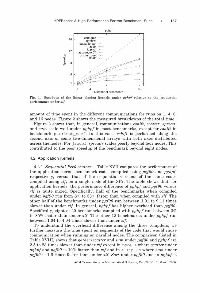
amount of time spent in the different communications for runs on 1, 4, 8,and 16 nodes. Figure 2 shows the measured breakdowns of the total time.

Figure 2 shows that, in general, communications cshift, scatter, spread,and sum scale well under pghpf in most benchmarks, except for cshift inbenchmark pcr:inst_coef . In this case, cshift is performed along thesecond axis of some two-dimensional arrays with both axes distributedacross the nodes. For jacobi , spreads scales poorly beyond four nodes. Thiscontributed to the poor speedup of the benchmark beyond eight nodes.

4.2 Application Kernels

4.2.1 Sequential Performance. Table XVII compares the performance ofthe application kernel benchmark codes compiled using pgf90 and pghpf,respectively, versus that of the sequential versions of the same codescompiled using xlf, on a single node of the SP2. The table shows that, forapplication kernels, the performance difference of pghpf and pgf90 versusxlf is quite mixed. Specifically, half of the benchmarks when compiledunder pgf90 run from 8% to 53% faster than when compiled with xlf. Theother half of the benchmarks under pgf90 run between 1.01 to 9.11 timesslower than under xlf. In general, pghpf has higher overhead than pgf90.Specifically, eight of 20 benchmarks compiled with pghpf run between 3%to 85% faster than under xlf. The other 12 benchmarks under pghpf runbetween 1.04 to 4.04 times slower than under xlf.

To understand the overhead difference among the three compilers, wefurther measure the time spent on segments of the code that would causecommunication when running on parallel nodes. The comparison (listed inTable XVIII) shows that gather/scatter and sum under pgf90 and pghpf are2.5 to 23 times slower than under xlf except in mdcell where scatter underpghpf and pgf90 is 10% faster than xlf and in ellip-2d where sum underpgf90 is 1.6 times faster than under xlf. Sort under pgf90 and in pghpf is

1

4

8

12

16

1 4 8 16

Spe

edup

Number of processors

pghpf

conj-gradqr:solve

gauss-jordanjacobi

lu:pivotmatrix-vector(4)

pcr:inst_coeffft-2D

Fig. 1. Speedups of the linear algebra kernels under pghpf relative to the sequentialperformance under xlf.



0

50

100

150

200

250

1 4 8 16

Tim

e (s

ec.)


conj-grad

totalcshift

10

20

30

40

50

60

1 4 8 16

Tim

e (s

ec.)


fft-2D

totalcshift

scatter

0

5

10

15

20

25

30

35

40

45

50

1 4 8 16

Tim

e (s

ec.)


gauss-jordan

totalspreadmaxloc

gather/scatter

0

20

40

60

80

100

120

1 4 8 16

Tim

e (s

ec.)


jacobi

totalspread

cshift

0

5

10

15

20

1 4 8 16

Tim

e (s

ec.)


lu:pivot

totalspreadmaxlocscatter

50

100

150

200

1 4 8 16

Tim

e (s

ec.)


matrix-vector(4)

totalsum

spread

0

2

4

6

8

10

12

14

16

1 4 8 16

Tim

e (s

ec.)


pcr:inst_coef

totalcshift

0

20

40

60

80

100

120

1 4 8 16

Tim

e (s

ec.)


qr:solve

totalsum

spread

Fig. 2. Total running time and the communication breakdowns for linear algebra bench-marks. For benchmarks with multiple cases only one case is shown.

138 • Y. C. Hu et al.


about 4 times slower than under xlf in qptransport , but is about the samein pic-gather/scatter under all three compilers.

4.2.2 Parallel Performance. Figure 3 shows the parallel speedups of theapplication benchmarks compiled using pghpf on up to 16 nodes of the SP2,using the performance of the sequential codes as the base. The applicationscan be divided into four groups according to their speedups. The first groupconsists of ellip-2d , which achieves better than linear speedup as aconsequence of 6.7 times better performance under pghpf than under xlfwith both running on one node. The much better performance with pghpf isdue much less cache conflicts from padding. The second group consists ofgmo, which achieves a linear speedup because of no communication. Thethird group consists of boson , ks-spectral , mdcell , md, pic-simple ,fem-3d , wave-1d, n-body:cshift-sym , n-body:cshift , step4 , qcd-kernel , and qmc. These benchmarks achieve from moderate to almostlinear speedups on up to 16 nodes. The last group consists of diff-3d ,pic-gather-scatter , n-body:bcast , n-body:spread , qptransport ,and rp . These benchmarks achieve fairly poor speedups. Among these fiveapplications, qptransport , pic-gather-scatter , and rp achieve poorspeedups as a result of their poor sequential performance when comparedwith xlf. The poor sequential performance is a result of the poor perfor-mance of gather/scatter, cshift, sort, and sum under pghpf than under xlf,as shown in Table XVIII.

Table XVII. Single-Node Performance of the Application Kernels

xlf pgf90 pghpf

Time FLOP Rate Time TimeCode (sec.) (Mflops/s) (vs. xlf) (vs. xlf)

boson 57.8 9.40 0.86 1.04diff-3d 43.7 41.2 0.47 1.42ellip-2d 96.5 6.79 0.88 0.15fem-3d 159.0 3.95 1.01 1.48gmo 107.0 14.4 0.94 0.99ks-spectral 116.0 1.97 0.70 0.85md 49.0 26.0 1.13 1.51mdcell 86.1 4.62 1.04 1.13n-body:bcast 100.0 45.5 0.62 0.97n-body:cshift 98.9 46.1 1.05 0.98n-body:cshift-sym 75.9 47.7 1.16 0.86n-body:spread 100.0 45.4 0.78 1.12pic-gather-scatter 24.6 4.80 2.22 4.03pic-simple 83.9 1.91 0.92 1.22qcd-kernel 37.9 33.5 1.11 1.37qmc 107.0 60.7 1.32 2.10qptransport 337.0 5.29 2.80 4.04rp 80.5 71.6 9.11 3.49step4 56.6 14.5 0.85 0.81wave-1d 54.9 1.90 0.70 0.90



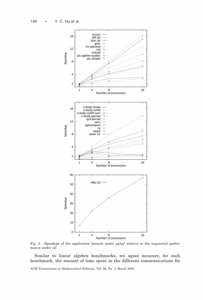
Similar to linear algebra benchmarks, we again measure, for eachbenchmark, the amount of time spent in the different communications for

1

4

8

12

16

1 4 8 16

Spe

edup


bosondiff-3d

fem-3dgmo

ks-spectralmd

mdcellpic-gather-scatter

pic-simple

1

4

8

12

16

1 4 8 16

Spe

edup


n-body:bcastn-body:cshift

n-body:cshift-symn-body:spread

qcd-kernelqmc

qptransportrp

step4wave-1d

0

10

20

30

40

50

60

1 4 8 16

Spe

edup


ellip-2d

Fig. 3. Speedups of the application kernels under pghpf relative to the sequential perfor-mance under xlf.

140 • Y. C. Hu et al.


runs on 1, 4, 8, and 16 nodes. Figures 4–6 show the measured breakdownsof the total time. For most applications, communications cshift, gather/scatter, sort, and sum scale well under pghpf till eight nodes. On the otherhand, communications broadcast and spread achieve slowdown beyond fournodes, as shown in n-body:bcast and n-body:spread .

4.3 Effect of Data Layouts

We also evaluate the effects of different data layouts on the benchmarkperformance under the HPF compiler pghpf. Specifically, the LU decompo-sition used in the lu benchmark and and QR factorization used in the qrbenchmark is well known to achieve better load balance with the cyclicarray layout than with block array layout. We measure the overall runningtime as well as the communication time breakdowns for lu:pivot andqr:solve with three distributions: block, cyclic, and block-cyclic with ablock size 4, respectively. The measurements are shown in Figures 7 and 8.

Table XVIII. Breakdown of the Single-Node Time of the Application Kernel Benchmarks


boson total 57.8 50.1 60.2cshift 2.90 9.44 3.57

diff-3d total 43.7 20.4 61.8ellip-2d total 96.5 84.6 14.4

cshift 87.7 49.5 5.86sum 2.46 1.54 2.55

fem-3d total 159.0 160.0 235.0gather 0.77 0.52 41.6scatter 3.02 32.7 39.3

gmo total 107.0 101.0 106.0ks-spectral total 116.2 81.6 98.5

scatter 0.41 6.15 7.46cshift 54.9 21.7 32.9

md total 49.0 55.1 74.1spread 5.91 5.53 6.03sum 3.11 24.1 34.7

mdcell total 86.1 89.2 97.7cshift 9.03 13.6 15.0scatter 2.27 1.99 2.06

n-body:bcast total 100.0 62.2 96.9broadcast 15.2 15.4 15.7

n-body:cshift total 98.9 103.0 97.2cshift 15.5 57.3 15.8

n-body:cshift-sym total 75.9 88.4 65.2cshift 13.0 43.0 13.4

n-body:spread total 100.0 77.6 112.4spread 15.6 31.0 31.3

pic-gather-scatter total 24.6 54.5 99.0sort 0.91 0.68 0.95scan 0.93 2.64 3.80gather 2.77 7.43 14.32scatter 1.06 12.5 18.5



Overall, The total running time using block-cyclic(4) distribution is about 2to 5.5 times longer than using block distribution on 1, 4, 8, and 16 nodes forboth benchmarks. Using pure cyclic distribution, the total running time isalmost identical to that using block distribution for qr:solve and is about2 to 2.5 times for lu:pivot . The fact that the performance gap on parallelnodes is consistent with that on one node suggests that the cause of the gapis again due to poor nodal compilation for cyclic distributions.

A close look at the communication time breakdowns shows that block-cyclic(4) distribution loses to block and cyclic distributions mainly in thespread communication on one node as well as on parallel nodes. Theblock-cyclic(4) distribution actually beats the pure cyclic distribution formaxloc and scatter communications as shown by lu:pivot . For qr:solve ,the pure cyclic distribution only loses to the block distribution on spread bya factor of two on parallel nodes.

5. SUMMARY

The HPFBench benchmark suite is a set of High Performance Fortrancodes intended for evaluating HPF compilers on scalable parallel architec-tures. The codes contain new constructs of Fortran 90 and HPF. Thebenchmarks cover several aspects of the array syntax of Fortran 90 andHPF, scientific software library functions, and application kernels thatreflect the computational structure and communication patterns in typicalscientific applications, particularly fluid dynamic simulations, fundamental

Table XVIII. Continued


pic-simple total 83.9 77.3 102.0sum_scatter 0.80 4.22 7.41copy_scatter 0.31 7.11 7.14cshift 32.1 21.2 24.1gather 1.11 1.11 19.3

qcd-kernel total 37.9 41.9 52.0cshift 6.00 8.82 9.13

qmc total 107.0 141.0 225.0scan 16.1 11.5 13.4scatter 3.71 33.8 87.9reduction 0.72 0.80 0.91

qptransport total 33.7 94.5 136.0sort 13.8 55.4 61.5scan 4.11 10.9 14.4scatter 7.42 18.8 40.4

rp total 80.5 735.0 282.0sum 4.01 67.1 6.01cshift 60.5 645.0 262.0

step4 total 56.6 48.0 46.0cshift 27.7 30.6 28.4

wave-1d total 54.9 38.6 49.2cshift 16.6 8.66 12.3scatter 0.72 1.93 2.84

142 • Y. C. Hu et al.


0

10

20

30

40

50

60

70

1 4 8 16

Tim

e (s

ec.)


boson

totalcshift

0

10

20

30

40

50

60

70

1 4 8 16

Tim

e (s

ec.)


diff-3d

total

0

2

4

6

8

10

12

14

16

1 4 8 16

Tim

e (s

ec.)


ellip-2d

totalcshift

reduction

0

50

100

150

200

1 4 8 16

Tim

e (s

ec.)


fem-3d

totalgatherscatter

20

40

60

80

100

120

1 4 8 16

Tim

e (s

ec.)


gmo

total

0

20

40

60

80

100

1 4 8 16

Tim

e (s

ec.)


ks-spectral

totalscatter

cshift

10

20

30

40

50

60

70

80

1 4 8 16

Tim

e (s

ec.)


md

totalspread

sum

0

20

40

60

80

100

1 4 8 16

Tim

e (s

ec.)


mdcell

totalcshift

scatter

Fig. 4. Total running time and the communication breakdowns for application kernelsboson , diff-3d , ellip-2d , fem-3d , gmo, ks-spectral , md, and mdcell .



0

20

40

60

80

100

120

1 4 8 16

Tim

e (s

ec.)


n-body

nb:bcast: totalnb:bcast: bcast

nb:cshift: totalnb:cshift: cshift

0

20

40

60

80

100

120

1 4 8 16

Tim

e (s

ec.)


n-body

nb:cshift-sym: totalnb:cshift-sym: cshift

nb:spread: totalnb:spread: spread

0

20

40

60

80

100

1 4 8 16

Tim

e (s

ec.)


pic-gather-scatter

totalsort

scanscattergather

20

40

60

80

100

1 4 8 16

Tim

e (s

ec.)


pic-simple

totalcshift

sum_scattercopy_scatter

gather

0

10

20

30

40

50

1 4 8 16

Tim

e (s

ec.)


qcd-kernel

totalcshift

50

100

150

200

250

1 4 8 16

Tim

e (s

ec.)


qmc

totalscan

scatterreduction

20

40

60

80

100

120

140

1 4 8 16

Tim

e (s

ec.)


qptransport

totalsort

scatterscan

50

100

150

200

250

300

1 4 8 16

Tim

e (s

ec.)


rp

totalcshiftsum

Fig. 5. Total running time and the communication breakdowns for application kernelsn-body , pic-gather-scatter , pic-simple , qcd-kernel , qmc, qptransport , and rp .

144 • Y. C. Hu et al.


physics, and molecular studies in chemistry or biology. We provide perfor-mance evaluation metrics in the form of elapsed times, FLOP rates, andcommunication time breakdowns, and quantify performance according tothe FLOP count, memory usage, communication pattern, local memoryaccess, as well as operation and communication counts per iteration. Wealso provide a benchmark guide to aid the choice of subsets of the bench-marks for evaluating particular aspects of an HPF compiler. We expect the

10

20

30

40

50

1 4 8 16

Tim

e (s

ec.)


step4

totalcshift

0

5

10

15

20

25

30

35

40

45

50

1 4 8 16

Tim

e (s

ec.)


wave-1d

totalcshift

scatter

Fig. 6. Total running time and the communication breakdowns for application kernels step4and wave-1d .

0

20

40

60

80

100

120

1 4 8 16

Tim

e (s

ec.)


block(4)-cyclic: totalcyclic: totalblock: total

0

10

20

30

40

50

60

1 4 8 16

Tim

e (s

ec.)


block(4)-cyclic: spreadcyclic: spreadblock: spread

0

2

4

6

8

10

1 4 8 16

Tim

e (s

ec.)


block(4)-cyclic: maxloccyclic: maxlocblock: maxloc

0

0.5

1

1.5

2

2.5

3

3.5

4

1 4 8 16

Tim

e (s

ec.)


block(4)-cyclic: scattercyclic: scatterblock: scatter

Fig. 7. Total running time and communication time breakdowns of lu:pivot under differentarray layouts. Note the different scale of the y-axis for the breakdowns.



HPFBench benchmark suite to be a valuable asset in the development andevaluation of Fortran 90 and HPF compilers.

We have reported a performance evaluation of an industry-leading HPFcompiler, pghpf, from the Portland Group Inc. using the HPFBench bench-marks on the distributed-memory IBM SP2. While with respect to runningthe HPF benchmarks on one node, most of the benchmarks achieved goodspeedups on up to 16 nodes of the SP2, over half of the 25 benchmarkscompiled using pghpf run over 10% slower than their Fortran 77 counter-parts compiled using the native F77 compiler xlf. Among these bench-marks, the gap is over a factor of two for five benchmarks. The measure-ment of communication time breakdowns shows that the high overheadwith pghpf when running on a single node mainly comes from the poornodal performance of these communications segments of the codes; thoughon one node, the data movement is all within the node.

ACKNOWLEDGMENTS

We would like to thank the anonymous referees and the Editor-in-ChiefRonald Boisvert for careful reading of the manuscript and providing uswith detailed comments which have greatly improved both the content andthe presentation of the article.

0

50

100

150

200

250

300

1 4 8 16T

ime

(sec

.)


block(4)-cyclic: totalcyclic: totalblock: total

0

20

40

60

80

100

1 4 8 16

Tim

e (s

ec.)


block(4)-cyclic: sumcyclic: sumblock: sum

0

10

20

30

40

50

60

1 4 8 16

Tim

e (s

ec.)


block(4)-cyclic: spreadcyclic: spreadblock: spread

Fig. 8. Total running time and communication time breakdowns of qr:solve under differentarray layouts. Note the different scale of the y-axis for the breakdowns.

146 • Y. C. Hu et al.


REFERENCES

ANDERSON, J., TRAYNOR, C., AND BOGHOSIAN, B. 1991. Quantum chemistry by random walk:Exact treatment of many-electon systems. J. Chem. Phys. 95, 10 (Nov.), 7418–7425.

AOKI, S., SHROCK, R., BERG, B., OGILVIE, M., PETCHER, D., BHANOT, G., ROSSI, P., BITAR, K.,EDWARDS, R., HELLER, U. M., KENNEDY, A., SANIELEVICI, S., BROWER, R., POTVIN, J., REBBI, C.,BROWN, F. R., CHRIST, N., MAWHINNEY, R., DETAR, C., DRAPER, T., LIU, K., GOTTLIEB, S.,HAMBER, H., KILCUP, G., SHIGEMITSU, J., KOGUT, J., KRONFELD, A., LEE, I. H., NEGELE, J.,OHTA, S., SEXTON, J. C., SHURYAK, E., SINCLAIR, D. K., SONI, A., AND WILCOX, W.1991. Physics goals of the QCD teraflop project. Int. J. Mod. Phys. C 2, 4 (Dec.), 829–947.

BAILEY, D. H. AND BARTON, J. 1985. The NAS kernel benchmark program. Tech. Memo.86711. RIACS, NASA Ames Research Center, Moffett Field, CA.

BAILEY, D., BARSZCZ, E., BARTON, E., BROWNING, D., CARTER, R., DAGUM, L., FATOOHI, R.,FINEBERG, S., FREDERICKSON, P., LASINSKI, T., SCHREIBER, T., SIMON, R., VENKATAKRISHNAN, V.,AND WEERATUNGA, S. 1994. The NAS parallel benchmarks. Tech. Rep.RNR-94-007. RIACS, NASA Ames Research Center, Moffett Field, CA.

BAILEY, D., HARRIS, T., SAPHIR, W., WIJNGAARTAND, R., WOO, A., AND YARROW, M. 1995. TheNAS parallel benchmarks 2.0. Tech. Rep. NAS-95-020. RIACS, NASA Ames ResearchCenter, Moffett Field, CA.

BATROUNI, G. AND SCALETTAR, R. 1992. World-line quantum Monte Carlo algorithm for aone-dimensional Bose model. Phys. Rev. B46, 14 (Oct.), 9051–9062.

BERRY, M., CHEN, D., KOSS, P., KUCK, D., LO, S., PANG, Y., POINTER, L., ROLOFF, R., SAMEH, A.,CLEMENTI, E., CHIN, S., SCHNEIDER, D., FOX, G., MESSINA, P., WALKER, D., HSIUNG, C.,SCHWARZMEIER, J., LUE, K., ORSZAG, S., SEIDL, F., JOHNSON, O., GOODRUM, R., AND MARTIN, J.1989. The PERFECT Club benchmarks: Effective performance evaluation of super-computers. Int. J. Supercomput. Appl. High Perform. Eng. 3, 1, 5–30.

BLACKFORD, L. S., CHOI, J., CLEARY, A., D’AZEVEDO, E., DEMMEL, J., DHILLON, I., DONGARRA, J.,HAMMARLING, S., HENRY, G., PETITET, A., STANLEY, K., WALKER, D., AND WHALEY, R. C.1997. Scalapack: A linear algebra library for message-passing computers. In Proceedings ofthe SIAM Conference on Parallel Processing (Mar.), SIAM, Philadelphia, PA.

BRAMLEY, R. AND SAMEH, A. 1992. Row projection methods for large nonsymmetric linearsystems. SIAM J. Sci. Stat. Comput. 13, 1 (Jan. 1992), 168–193.

BRICKNER, R. G., GEORGE, W., JOHNSSON, S. L., AND RUTTENBERG, A. 1993. A stencil compilerfor the Connection Machine models CM-2/200. In Proceedings of the 4th InternationalWorkshop on Compilers for Parallel Computers, H. Sips, Ed. Delft University of Technology,Delft, The Netherlands, 68–78.

CIMMINO, G. 1939. Calcolo approssimato per le soluzioni dei sistemi di equazioni lineari. Ric.Sci. Progr. Tecn. Econom. Naz. 9, 326–333.

COOLEY, J. C. AND TUCKEY, J. 1965. An algorithm for the machine computation of complexFourier series. Math. Comput. 19, 291–301.

CYBENKO, G., KIPP, L., POINTER, L., AND KUCK, D. 1990. Supercomputer performanceevaluation and the Perfect Benchmarks. In Proceedings of the 1990 ACM InternationalConference on Supercomputing (ICS ’90, Amsterdam, The Netherlands, June 11–15), A.Sameh and H. van der Vorst, Eds. ACM Press, New York, NY, 254–266.

DAHLQUIST, G., BJÖRCK, A., AND ANDERSON, N. 1974. Numerical Methods. Prentice-Hall Seriesin Automatic Computation. Prentice-Hall, Englewood Cliffs, NJ.

DEKKER, T. AND HOFFMAN, W. 1989. Rehabilitation of the Gauss-Jordan algorithm. Numer.Math. 54, 4, 591–599.

DONGARRA, J. J. 1989. Performance of various computers using standard linear equationssoftware. Tech. Rep. CS-89-85. Department of Computer Science, University of Tennessee,Knoxville, TN.

DONGARRA, J., MARTIN, J., AND VORLTON, J. 1987. Computer benchmarking: Paths andpitfalls. IEEE Spectrum 24, 7 (July 1987), 38–43.

GEORGE, W., BRICKNER, R. G., AND JOHNSSON, S. L. 1994. POLYSHIFT communicationssoftware for the connection machine system CM-200. Sci. Program. 3, 1 (Spring), 83–99.



GOLUB, G. AND VAN LOAN, C. F. 1989. Matrix Computations. 2nd ed. Johns HopkinsUniversity Press, Baltimore, MD.

GREENBERG, A., MESIROV, J., AND SETHIAN, J. 1992. Programming direct N-body solvers onConnection Machines. Tech. Rep. 245. Thinking Machines Corp., Bedford, MA.

HENNESSY, J. L. AND PATTERSON, D. A. 1990. Computer Architecture: A QuantitativeApproach. Morgan Kaufmann Publishers Inc., San Francisco, CA.

HIGH PERFORMANCE FORTRAN FORUM. 1993. High Performance Fortran; language specifica-tion, version 1.0. Sci. Program. 2, 1-2, 1–170.

HIGH PERFORMANCE FORTRAN FORUM. 1997. High Performance Fortran language specification,version 2.0. Rice University, Houston, TX. http://dacnet.rice.edu/Depts/CRPC/HPFF/versions/hpf2/hpf2-v20/index.html.

HIRSCH, J., SUGAR, R., SCALAPINO, D., AND BLANKENBECLER, R. 1982. Monte Carlo simulationsof one-dimensional Fermion systems. Phys. Rev. B26, 9 (Nov.), 5033–5055.

HO, C.-T. AND JOHNSSON, S. L. 1990. Optimizing tridiagonal solvers for alternating directionmethods on Boolean cube multiprocessors. SIAM J. Sci. Stat. Comput. 11, 3 (May 1990),563–592.

HOCKNEY, R. W. 1965. A fast direct solution of Poisson’s equation using Fourier analysis. J.ACM 12, 1, 95–113.

HOCKNEY, R. AND BERRY, M. 1994. Public international benchmarks for parallel computers:Parkbench committee report-1. Tech. Rep. Oak Ridge National Laboratory, Oak Ridge, TN.

HOCKNEY, R. W. AND EASTWOOD, J. W. 1988. Computer Simulation Using Particles. Taylorand Francis, Inc., Bristol, PA.

HOCKNEY, R. W. AND JESSHOPE, C. 1988. Parallel Computers 2. Adam Hilger.HU, Y. AND JOHNSSON, S. L. 1996. Implementing O~N! N-body algorithms efficiently in

data-parallel languages. Sci. Program. 5, 4, 337–364.HU, Y. C. AND JOHNSSON, S. L. 1999. Data parallel performance optimizations using array

aliasing. In Algorithms for Parallel Processing, M. Heath, A. Ranade, and R. Schreiber, Eds.IMA Volumes in Mathematics and Its Applications, vol. 105. Springer-Verlag, Vienna,Austria, 213–245.

HU, Y. C., JOHNSSON, S. L., AND TENG, S.-H. 1997. High Performance Fortran for highlyirregular problems. In Proceedings of the 6th ACM Symposium on Principles and Practice ofParallel Programming (SIGPLAN ’97, Las Vegas, NV, June 18–21), M. A. Berman, Ed.ACM Press, New York, NY.

IBM. 1996. IBM Parallel Engineering and Scientific Subroutine Library Release 2, Guide andReference. IBM Corp., Riverton, NJ.

JOHNSON, C. 1987. Numerical Solutions of Partial Differential Equations by Finite ElementMethod. Cambridge University Press, New York, NY.

JOHNSON, C. AND SZEPESSY, A. 1987. On the convergence of a finite element method for anonlinear hyperbolic conservation law. Math. Comput. 49, 180, 427–444.

JOHNSSON, S. L. 1985. Solving narrow banded systems on ensemble architectures. ACMTrans. Math. Softw. 11, 3 (Sept. 1985), 271–288.

JOHNSSON, S. L. AND HO, C.-T. 1989. Optimum broadcasting and personalized communicationin hypercubes. IEEE Trans. Comput. 38, 9 (Sept.), 1249–1268.

JOHNSSON, S. L., HARRIS, T., AND MATHUR, K. K. 1989. Matrix multiplication on the connectionmachine. In Proceedings of the 1989 Conference on Supercomputing (Reno, NV, Nov. 13–17,1989), F. R. Bailey, Ed. ACM Press, New York, NY, 326–332.

JOHNSSON, S. L., JACQUEMIN, M., AND KRAWITZ, R. L. 1992. Communication efficientmulti-processor FFT. J. Comput. Phys. 102, 2 (Oct.), 381–387.

LOMDAHL, P. S., TAMAYO, P., GRØNBECH-JENSEN, N., AND BEAZLEY, D. M. 1993. 50 GFlopsmolecular dynamics on the Connection Machine 5. In Proceedings of the Conference onSupercomputing (Supercomputing ’93, Portland, OR, Nov. 15–19), B. Borchers and D.Crawford, Eds. IEEE Computer Society Press, Los Alamitos, CA, 520–527.

LUBECK, O., MOORE, J., AND MENDEZ, R. 1985. A benchmark comparison of three supercom-puters: Fujitsu vp-200, hitachi s810/20, and cray x-mp/2. IEEE Computer 18, 12, 10–24.

148 • Y. C. Hu et al.


MCMAHON, F. 1988. The Livermore Fortran kernels: A test of numerical performancerange. In Performance Evaluation of Supercomputers, J. L. Martin, Ed. Elsevier North-Holland, Inc., New York, NY, 143–186.

OLSSON, P. 1994. The numerical behavior of high-order finite difference methods. J. Sci.Comput. 9, 4 (Dec. 1994), 445–466.

OLSSON, P. 1995a. Summation by parts, projections, and stability. I. Math. Comput. 64, 211(July 1995), 1035–1065.

OLSSON, P. 1995b. Summation by parts, projections, and stability. II. Math. Comput. 64, 212(Oct. 1995), 1473–1493.

PRESS, W. H., TEUKOLSKY, S. A., VETTERLING, W. T., AND FLANNERY, B. P. 1992. NumericalRecipes in C: The Art of Scientific Computing. 2nd ed. Cambridge University Press, NewYork, NY.

SCHROFF, G. AND SCHREIBER, R. 1988. On the convergence of the cyclic Jacobi method forparallel block orderings. Tech. Rep. 88-11. Computer Science Deptartment, RensselaerPolytechnic Institute, Troy, NY.

SINVHAL-SHARMA, P., RAUCHWERGER, L., AND LARSON, J. 1991. Perfect benchmarks: Instru-mented version. Tech. Rep. CSRD-TR-1152.

TOBOCHNIK, J., BATROUNI, G. G., AND GOULD, H. 1992. Quantum Monte Carlo on alattice. Comput. Phys. 6, 6 (Nov.-Dec.), 673–680.

TRAYNOR, C., ANDERSON, J., AND BOGHOSIAN, B. 1991. A quantum Monte Carlo calculation ofthe ground state energy of the hydrogen molecule. J. Chem. Phys. 94, 5 (Mar.), 3567–3664.

WILKINSON, J. 1961. Error analysis of direct methods of matrix inversion. J. ACM 8, 3 (July),281–330.

WUELLER-WICHARDS, D. AND GENTZSCH, W. 1982. Performance comparisons among severalparallel and vector computers on a set of fluid flow problems. Tech. Rep. IB 262-82 R01.

Received: November 1996; revised: July 1998, October 1999, and November 1999; accepted:November 1999



hpfbench: a high performance fortran benchmark suiteychu/publications/hpfbench.pdf · ......

Documents