hspice essentials workshop - iran university of science ...een.iust.ac.ir/profs/abrishamifar/analog...
TRANSCRIPT

C U S TO ME R E D U C A TI O N S E R V I C E S
HSPICE Essentials
Workshop
Student Guide 60-I-031-BSG-008 2007.03
Synopsys Customer Education Services
700 East Middlefield Road
Mountain View, California 94043
Workshop Registration: 1-800-793-3448
www.synopsys.com

Synopsys Customer Education Services
Copyright Notice and Proprietary Information Copyright 2007 Synopsys, Inc. All rights reserved. This software and documentation contain confidential and proprietary information that is the property of Synopsys, Inc. The software and documentation are furnished under a license agreement and may be used or copied only in accordance with the terms of the license agreement. No part of the software and documentation may be reproduced, transmitted, or translated, in any form or by any means, electronic, mechanical, manual, optical, or otherwise, without prior written permission of Synopsys, Inc., or as expressly provided by the license agreement.
Right to Copy Documentation The license agreement with Synopsys permits licensee to make copies of the documentation for its internal use only. Each copy shall include all copyrights, trademarks, service marks, and proprietary rights notices, if any. Licensee must assign sequential numbers to all copies. These copies shall contain the following legend on the cover page: “This document is duplicated with the permission of Synopsys, Inc., for the exclusive use of __________________________________________ and its employees. This is copy number __________.”
Destination Control Statement All technical data contained in this publication is subject to the export control laws of the United States of America. Disclosure to nationals of other countries contrary to United States law is prohibited. It is the reader’s responsibility to determine the applicable regulations and to comply with them.
Disclaimer SYNOPSYS, INC., AND ITS LICENSORS MAKE NO WARRANTY OF ANY KIND, EXPRESS OR IMPLIED, WITH REGARD TO THIS MATERIAL, INCLUDING, BUT NOT LIMITED TO, THE IMPLIED WARRANTIES OF MERCHANTABILITY AND FITNESS FOR A PARTICULAR PURPOSE.
Registered Trademarks (®) Synopsys, AMPS, Cadabra, CATS, CRITIC, CSim, Design Compiler, DesignPower, DesignWare, EPIC, Formality, HSIM, HSPICE, iN-Phase, in-Sync, Leda, MAST, ModelTools, NanoSim, OpenVera, PathMill, Photolynx, Physical Compiler, PrimeTime, SiVL, SNUG, SolvNet, System Compiler, TetraMAX, VCS, Vera, and YIELDirector are registered trademarks of Synopsys, Inc.
Trademarks (™) AFGen, Apollo, Astro, Astro-Rail, Astro-Xtalk, Aurora, AvanWaves, Columbia,Columbia-CE, Cosmos, CosmosEnterprise, CosmosLE, CosmosScope, CosmosSE, DC Expert, DC Professional, DC Ultra, Design Analyzer, Design Vision, DesignerHDL, Direct Silicon Access, Discovery, Encore, Galaxy, HANEX, HDL Compiler, Hercules, Hierarchical Optimization Technology, HSIMplus, HSPICE-Link, iN-Tandem, i-Virtual Stepper, Jupiter, Jupiter-DP, JupiterXT, JupiterXT-ASIC, Liberty, Libra-Passport,Library Compiler, Magellan, Mars, Mars-Rail, Milkyway, ModelSource, Module Compiler, Planet, Planet-PL, Polaris, Power Compiler, Raphael, Raphael-NES,Saturn, Scirocco, Scirocco-i, Star-RCXT, Star-SimXT, Taurus, TSUPREM-4, VCS Express, VCSi, VHDL Compiler, VirSim, and VMC are trademarks of Synopsys, Inc.
Service Marks (SM) MAP-in, SVP Café, and TAP-in are service marks of Synopsys, Inc. SystemC is a trademark of the Open SystemC Initiative and is used under license. ARM and AMBA are registered trademarks of ARM Limited. Saber is a registered trademark of SabreMark Limited Partnership and is used under license. All other product or company names may be trademarks of their respective owners. Document Order Number: 60-I-031-BSG-008 HSPICE Essentials Student Guide

Table of Contents
Synopsys 60-I-031-BSG-008 i HSPICE Essentials
Unit i: Introduction & Overview
Introductions ..................................................................................................................... i-2
Facilities............................................................................................................................ i-3
Workshop Goal ................................................................................................................. i-4
Target Audience................................................................................................................ i-5
Agenda: Day 1................................................................................................................... i-6
Workshop Objectives: Day 1 ............................................................................................ i-7
Agenda: Day 2................................................................................................................... i-8
Workshop Objectives: Day 2 ............................................................................................ i-9
Icons Used in this Workshop .......................................................................................... i-10
Unit 1: Introduction
Unit Objectives ................................................................................................................ 1-2
Introduction...................................................................................................................... 1-3
History of SPICE ............................................................................................................. 1-4
History of SPICE ............................................................................................................. 1-5
History of HSPICE........................................................................................................... 1-6
Rules of Simulation ......................................................................................................... 1-7
Simulation Goals.............................................................................................................. 1-8
Simulation Takes Place.................................................................................................... 1-9
Silicon to HDL............................................................................................................... 1-10
Simulation and Analysis ................................................................................................ 1-11
HSPICE Fundamentals .................................................................................................. 1-12
Files and Suffixes........................................................................................................... 1-13
Starting HSPICE ............................................................................................................ 1-14
Netlist Structure ............................................................................................................. 1-15
Netlist Structure: Overview ........................................................................................... 1-16
Netlist Structure: Topology............................................................................................ 1-17
Node Naming Conventions (1/2) ................................................................................... 1-18
Node Naming Conventions (2/2) ................................................................................... 1-19
Element Naming Conventions ....................................................................................... 1-20
Units and Scale Factors.................................................................................................. 1-21
Passive Components: Resistor ....................................................................................... 1-22
Passive Components: Inductor....................................................................................... 1-23
Passive Components: Capacitor..................................................................................... 1-24
Sources ......................................................................................................................... 1-25
Independent Sources: DC, AC (1/2) .............................................................................. 1-26
Independent Sources (2/2) ............................................................................................. 1-27
Independent Transient Sources: Pulse .......................................................................... 1-28
Pulse Example................................................................................................................ 1-29
Independent Transient Sources: PWL........................................................................... 1-30

Table of Contents
Synopsys 60-I-031-BSG-008 ii HSPICE Essentials
PWL Example................................................................................................................ 1-31
Independent Transient Sources: PAT ............................................................................ 1-32
Independent Transient Sources: PRBS .......................................................................... 1-33
Independent Transient Sources: SIN.............................................................................. 1-34
Mixed Independent Sources........................................................................................... 1-35
Dependent Sources (1/3)................................................................................................ 1-36
Dependent Sources (2/3)................................................................................................ 1-37
Dependent Sources (3/3)................................................................................................ 1-38
Dependent Source Examples ......................................................................................... 1-39
Discovery AMS Simulation Interface Basics................................................................. 1-40
Discovery AMS Simulation Interface............................................................................ 1-41
Discovery AMS Simulation Interface – Project Management....................................... 1-42
Discovery AMS Simulation Interface – Project Management....................................... 1-43
Discovery AMS Simulation Interface – Setup............................................................... 1-44
Discovery AMS Simulation Interface – Netlist & Simulation....................................... 1-45
Discovery AMS Simulation Interface – Netlist & Simulation....................................... 1-46
Discovery AMS Simulation Interface – HSPICE Setup ................................................ 1-47
Discovery AMS Simulation Interface – HSPICE Setup ................................................ 1-48
Discovery AMS Simulation Interface – Run ................................................................. 1-49
Discovery AMS Simulation Interface – Run ................................................................. 1-50
Discovery AMS Simulation Interface - Output ............................................................. 1-51
Discovery AMS Simulation Interface - Simulation ....................................................... 1-52
Invoking CosmosScope.................................................................................................. 1-53
CosmosScope Basics ..................................................................................................... 1-54
CosmosScope Pulldown Menu Bar ............................................................................... 1-55
CosmosScope Icon Bar .................................................................................................. 1-56
CosmosScope Tool Bar.................................................................................................. 1-57
CosmosScope Mouse Usage .......................................................................................... 1-58
Opening a Plotfile .......................................................................................................... 1-59
CosmosScope File/Signal Control Forms...................................................................... 1-60
Scope Plotting Techniques (1/2) .................................................................................... 1-61
Scope Plotting Techniques (2/2) .................................................................................... 1-62
CosmosScope Measurements......................................................................................... 1-63
CosmosScope Measurements......................................................................................... 1-64
CosmosScope Measurements......................................................................................... 1-65
CosmosScope Calculator ............................................................................................... 1-66
Using the Calculator ...................................................................................................... 1-67
Lab 1: HSPICE............................................................................................................... 1-68
Unit 2: Active Devices / Analysis
Unit Objectives ................................................................................................................ 2-2

Table of Contents
Synopsys 60-I-031-BSG-008 iii HSPICE Essentials
Active Devices and Analysis Types................................................................................. 2-3
Components: Diodes (1/2) ............................................................................................... 2-4
Components: Diodes (2/2) ............................................................................................... 2-5
Components: MOS Transistor ......................................................................................... 2-6
Components: MOS Transistor Model.............................................................................. 2-7
Components: JFET/MESFET .......................................................................................... 2-8
Components: JFET/MESFET Model............................................................................... 2-9
Components: BJT Transistor ......................................................................................... 2-10
BJT Transistor Model .................................................................................................... 2-11
Components: Subcircuits ............................................................................................... 2-12
Components: Subcircuit Calls ....................................................................................... 2-13
Components: Subcircuit Example ................................................................................. 2-14
Global Statement............................................................................................................ 2-15
Introduction to Verilog-A .............................................................................................. 2-16
Feature Overview .......................................................................................................... 2-17
Verilog-A Usage Overview ........................................................................................... 2-18
Loading Verilog-A Files ............................................................................................... 2-19
Instantiation Syntax........................................................................................................ 2-20
Verilog-A Model Cards ................................................................................................ 2-21
Instantiation Examples (1/2) .......................................................................................... 2-22
Instantiation Examples (2/2) .......................................................................................... 2-23
Parameter Case Sensitivity............................................................................................. 2-24
Output Control ............................................................................................................... 2-25
Output Control Examples ............................................................................................. 2-26
Verilog-A Examples .................................................................................................... 2-27
Analysis Types: Types and Order .................................................................................. 2-28
Analysis Types: DC Operating Point (1/2) .................................................................... 2-29
Analysis Types: DC Operating Point (2/2) .................................................................... 2-30
Analysis Types: DC Analysis ........................................................................................ 2-31
Analysis Types: DC Analysis Syntax (1/2).................................................................... 2-32
Analysis Types: DC Analysis Syntax (2/2).................................................................... 2-33
Analysis Types: AC Analysis ........................................................................................ 2-34
Analysis Types: AC Analysis Syntax ............................................................................ 2-35
Analysis Types: Other AC Analyses.............................................................................. 2-36
Analysis Types: Transient Analysis (1/3) ...................................................................... 2-37
Analysis Types: Transient Analysis (2/3) ...................................................................... 2-38
Analysis Types: Transient Analysis (3/3) ...................................................................... 2-39
Analysis Types: Other Transient Analyses .................................................................... 2-40
Analysis Types: Temperature Analysis.......................................................................... 2-41
Analysis Types: Temperature Analysis Example .......................................................... 2-42
Output and Formatting................................................................................................... 2-43
Output Commands (1/2) ................................................................................................ 2-44
Output Commands (2/2) ................................................................................................ 2-45
Output and Formatting: .PROBE/.PRINT (1/2)............................................................. 2-46

Table of Contents
Synopsys 60-I-031-BSG-008 iv HSPICE Essentials
Output and Formatting: .PROBE/.PRINT (2/2)............................................................. 2-47
Using .PROBE/.PRINT with Subcircuits ...................................................................... 2-48
Output Format: Analysis Data (1/2)............................................................................... 2-49
Output Format: Analysis Data (2/2)............................................................................... 2-50
Output Waveform Display............................................................................................. 2-51
Output Variables ............................................................................................................ 2-52
Output Variables: DC and Transient (1/2)..................................................................... 2-53
Output Variables: DC and Transient (2/2)..................................................................... 2-54
Output Variables: AC .................................................................................................... 2-55
Using ACOUT Option (1/3) .......................................................................................... 2-56
Using ACOUT Option (2/3) .......................................................................................... 2-57
Using ACOUT Option (3/3) .......................................................................................... 2-58
Output Variables: Element Templates ........................................................................... 2-59
Output Variables: .MEASURE...................................................................................... 2-60
Output Variables: Parametric Output............................................................................. 2-61
LAB 2: Devices and Subcircuits .................................................................................... 2-62
Unit 3: Controls and Options
Unit Objectives ................................................................................................................ 3-2
Overview of Options........................................................................................................ 3-3
Commonly Used Options ................................................................................................ 3-4
Understanding Options (1/2)............................................................................................ 3-5
Understanding Options (2/2)............................................................................................ 3-6
General Options: Listing File Options (1/5) .................................................................... 3-7
General Options: Listing File Options (2/5) .................................................................... 3-8
General Options: Listing File Options (3/5) .................................................................... 3-9
General Options: Listing File Options (4/5) .................................................................. 3-10
General Options: Listing File Options (5/5) .................................................................. 3-11
General Options: Netlist Options SCALE (1/2) ........................................................... 3-12
General Options: Netlist Options SCALE (2/2) .......................................................... 3-13
General Options: Model Options SCALM (1/2)........................................................... 3-14
General Options: Model Options SCALM (2/2)........................................................... 3-15
General Options: Output Control (1/2) .......................................................................... 3-16
General Options: Output Control (2/2) .......................................................................... 3-17
General Options: Performance Improvement (1/3)........................................................ 3-18
General Options: Performance Improvement (2/3)........................................................ 3-19
General Options: Performance Improvement (3/3)........................................................ 3-20
OP and DC Simulation Controls (1/3) ........................................................................... 3-21
OP and DC Simulation Control (2/3) ............................................................................ 3-22
OP and DC Simulation Controls (3/3) ........................................................................... 3-23
Transient Simulation Controls: RUNLVL (1/2) ............................................................ 3-24
Transient Simulation Controls: RUNLVL (2/2) ............................................................ 3-25

Table of Contents
Synopsys 60-I-031-BSG-008 v HSPICE Essentials
Transient Simulation Controls ....................................................................................... 3-26
LAB 3: Simulation Controls and Options...................................................................... 3-27
Unit 4: How Simulation Works
Unit Objectives ................................................................................................................ 4-2
Simulation Controls and Convergence ............................................................................ 4-3
How Simulation Works (1/2)........................................................................................... 4-4
How Simulation Works (2/2)........................................................................................... 4-5
The Matrix (1/2)............................................................................................................... 4-6
The Matrix (2/2)............................................................................................................... 4-7
Introduction of Nonlinear Elements (1/3) ........................................................................ 4-8
Introduction of Nonlinear Elements (2/3) ........................................................................ 4-9
Introduction of Nonlinear Elements (3/3) ...................................................................... 4-10
Linear vs. Small Signal Model....................................................................................... 4-11
Linearization (1/2).......................................................................................................... 4-12
Linearization (2/2).......................................................................................................... 4-13
Newton-Raphson: Solving the Matrix (1/2) .................................................................. 4-14
Newton-Raphson: Solving the Matrix (2/2) .................................................................. 4-15
Newton-Raphson Method .............................................................................................. 4-16
Newton-Raphson: Solving the Matrix (1/2) .................................................................. 4-17
Newton-Raphson: Solving the Matrix (2/2) .................................................................. 4-18
Newton-Raphson: Termination Criteria (1/2)................................................................ 4-19
Newton-Raphson: Termination Criteria (2/2)................................................................ 4-20
What is Non-convergence? ............................................................................................ 4-21
Non-convergence ........................................................................................................... 4-22
Non-convergence - General Aids (1/2) .......................................................................... 4-23
Non-convergence - General Aids (2/2) .......................................................................... 4-24
Convergence: Tolerances (1/3) ...................................................................................... 4-25
Convergence: Tolerances (2/3) ...................................................................................... 4-26
Convergence: Tolerances (3/3) ...................................................................................... 4-27
Convergence: Conductance Values (1/2)....................................................................... 4-28
Convergence: Conductance Values (2/2)....................................................................... 4-29
Convergence: Diode Resistance (1/2)............................................................................ 4-30
Convergence: Diode Resistance (2/2)............................................................................ 4-31
Non-convergence-General Aids: Summary ................................................................... 4-32
Four Basic Simulation Types......................................................................................... 4-33
DC Bias Point ................................................................................................................ 4-34
DC Non-Convergence.................................................................................................... 4-35
DC Bias Point Convergence Aids.................................................................................. 4-36
DC Auto-convergence Process (1/5).............................................................................. 4-37
DC Auto-convergence Process (2/5).............................................................................. 4-38
DC Auto-convergence Process (3/5).............................................................................. 4-39
Table of Contents
Synopsys 60-I-031-BSG-008 vi HSPICE Essentials
DC Auto-convergence Process (4/5).............................................................................. 4-40
DC Auto-convergence Process (5/5).............................................................................. 4-41
DC Bias Point: .NODESET and .IC (1/2)...................................................................... 4-42
DC Bias Point: .NODESET and .IC (2/2)...................................................................... 4-43
DC Bias Point: Symbolic Operating Point..................................................................... 4-44
DC Bias Point: Model Related (1/2).............................................................................. 4-45
DC Bias Point: Model Related (2/2).............................................................................. 4-46
Analysis Options: DIAGNOSTIC.................................................................................. 4-47
DC Bias Point: Summary............................................................................................... 4-48
LAB 4: DC Bias Point ................................................................................................... 4-49
Unit 5: Convergence
Unit Objectives ................................................................................................................ 5-2
DC Sweep and Convergence Aids ................................................................................... 5-3
DC Sweep: Rapid Transitions.......................................................................................... 5-4
DC Iteration Controls....................................................................................................... 5-5
DC Sweep: Discontinuities (1/3) ..................................................................................... 5-6
DC Sweep: Discontinuities (2/3) ..................................................................................... 5-7
DC Sweep: Discontinuities (3/3) ..................................................................................... 5-8
DC Sweep Analysis: Summary........................................................................................ 5-9
AC Sweep and Convergence Aids ................................................................................. 5-10
Transient and Convergence Aids ................................................................................... 5-11
Transient Analysis: General........................................................................................... 5-12
Transient Analysis: Timestep Control ........................................................................... 5-13
Dynamic Timestep Control Algorithms (1/3) ................................................................ 5-14
Dynamic Timestep Control Algorithms (2/3) ................................................................ 5-15
Dynamic Timestep Control Algorithms (3/3) ................................................................ 5-16
Transient: Non-convergence (1/2) ................................................................................. 5-17
Transient: Non-convergence (2/2) ................................................................................. 5-18
Transient Analysis: Corrective Actions (1/4) ................................................................ 5-19
Transient Analysis: Corrective Actions (2/4) ............................................................... 5-20
Transient Analysis: Corrective Actions (3/4) ............................................................... 5-21
Transient Analysis: Corrective Actions (4/4) ................................................................ 5-22
Transient Analysis: Summary........................................................................................ 5-23
Numeric Integration ....................................................................................................... 5-24
Numeric Integration Methods ........................................................................................ 5-25
Numeric Integration Issues (1/4).................................................................................... 5-26
Numeric Integration Issues (2/4).................................................................................... 5-27
Numeric Integration Issues (3/4).................................................................................... 5-28
Numeric Integration Issues (4/4).................................................................................... 5-29
Selecting Integration Methods ....................................................................................... 5-30
Numeric Integration Comparisons (1/3) ........................................................................ 5-31

Table of Contents
Synopsys 60-I-031-BSG-008 vii HSPICE Essentials
Numeric Integration Comparisons (2/3) ........................................................................ 5-32
Numeric Integration Comparisons (3/3) ........................................................................ 5-33
LAB 5: HSPICE Converges........................................................................................... 5-34
Unit 6: Advanced Input Elements
Unit Objectives ................................................................................................................ 6-2
Advanced Input File Elements ......................................................................................... 6-3
Parameters........................................................................................................................ 6-4
Parameters: Rules (1/2) ................................................................................................... 6-5
Parameters: Rules (2/2) .................................................................................................. 6-6
Using Parameters (1/2) .................................................................................................... 6-7
Using Parameters (2/2)..................................................................................................... 6-8
Parameters: Passing .IC to Subcircuits ............................................................................ 6-9
Parameters: Flexibility and Productivity........................................................................ 6-10
Corner Process Model Example..................................................................................... 6-11
Algebraics (1/2).............................................................................................................. 6-12
Algebraics (2/2).............................................................................................................. 6-13
Functions........................................................................................................................ 6-14
.MEASURE ................................................................................................................... 6-15
.MEASURE: Rise/Fall (1/2) ......................................................................................... 6-16
.MEASURE: Rise/Fall (2/2) ......................................................................................... 6-17
.MEASURE: AVG, RMS, MIN, MAX, PP (1/2) .......................................................... 6-18
.MEASURE: AVG, RMS, MIN, MAX, PP (2/2) .......................................................... 6-19
.MEASURE: FIND-WHEN........................................................................................... 6-20
.MEASURE: FIND-WHEN Examples .......................................................................... 6-21
.MEASURE: Equation Evaluation................................................................................. 6-22
.MEASURE: Derivative Function ................................................................................. 6-23
.MEASURE: Integral Function...................................................................................... 6-24
Standalone Measure Utility............................................................................................ 6-25
Measure File Example ................................................................................................... 6-26
.ALTER: Description ..................................................................................................... 6-27
.ALTER: Limitations ..................................................................................................... 6-28
.ALTER: .option ALTCC (1/2)...................................................................................... 6-29
.ALTER: .option ALTCC (2/2)...................................................................................... 6-30
.ALTER: Example ......................................................................................................... 6-31
Worst Case Analysis (1/2) ............................................................................................. 6-32
Worst Case Analysis (2/2) ............................................................................................. 6-33
.BIASCHK Statement .................................................................................................... 6-34
.BIASCHK Options ....................................................................................................... 6-35
.BIASCHK Keywords (1/3) ........................................................................................... 6-36
.BIASCHK Keywords (2/3) ........................................................................................... 6-37
.BIASCHK Keywords (3/3) ........................................................................................... 6-38

Table of Contents
Synopsys 60-I-031-BSG-008 viii HSPICE Essentials
.BIASCHK Element and Model Monitor Syntax .......................................................... 6-39
.BIASCHK Expression Monitor Syntax ........................................................................ 6-40
.BIASCHK MOS Region Monitor Syntax..................................................................... 6-41
.BIASCHK MOS Device Size Monitor Syntax ............................................................. 6-42
.BIASCHK Report – Minimum Bias Value (1/2).......................................................... 6-43
.BIASCHK Report – Minimum Bias Value (2/2).......................................................... 6-44
Lab 6: Advanced Input File Elements ........................................................................... 6-45
Customer Support
Synopsys Support Resources ........................................................................................ CS-2
SolvNet Online Support Offers:.................................................................................... CS-3
SolvNet Registration is Easy......................................................................................... CS-4
Support Center: AE-based Support............................................................................... CS-5
Other Technical Sources ............................................................................................... CS-6
Summary: Getting Support ........................................................................................... CS-7

Introduction & OverviewHSPICE Essentials
i-1© 2007
HSPICE Essentials
Synopsys Customer Education Services© 2007 Synopsys, Inc. All Rights Reserved Synopsys 60-I-031-BSG-008
The Golden Standard for Accurate Circuit Simulation
Introduction & OverviewHSPICE Essentials
i-2© 2007
2i-
Introductions
� Name
� Company
� Job responsibilities
� EDA experience
� Main goals and expectations for this course
EDA = Electronic Design Automation
Introduction & OverviewHSPICE Essentials
i-3© 2007
3i-
Facilities
Building Hours
Restrooms
Meals
Messages
Smoking
Recycling
Phones
Emergency EXIT
Please turn off cell phones and pagers

Introduction & OverviewHSPICE Essentials
i-4© 2007
4i-
Workshop Goal
Prepare the student to useHSPICE for analog simulation and analysis in a silicon to HDL flow.
Introduction & OverviewHSPICE Essentials
i-5© 2007
5i-
Target Audience
Analog designers and engineers who
perform circuit simulation and analysis at the transistor level.

Introduction & OverviewHSPICE Essentials
i-6© 2007
6i-
Agenda: Day 1
Introduction1
Active Devices / Analysis2
Controls and Options3
DAY
1111
How Simulation Works4

Introduction & OverviewHSPICE Essentials
i-7© 2007
7i-
Workshop Objectives: Day 1
� List the goals of simulation
� Explain the HSPICE file structure
� List the HSPICE output files
� Use passive components and independent sources to construct a netlist
� Use active devices and subcircuits in a netlist
� Name the available types of analysis
� Explain how to output the simulation results
� Invoke and use CosmosScope andthe Discovery AMS Simulation Interface
� Use simulation controls and options
� Describe convergence and non-convergence
� Explain how the DC operating point is calculated

Introduction & OverviewHSPICE Essentials
i-8© 2007
8i-
Agenda: Day 2
Convergence5
Advanced Input Elements6
DAY
2222
Customer SupportCS

Introduction & OverviewHSPICE Essentials
i-9© 2007
9i-
Workshop Objectives: Day 2
� Describe DC sweep and transient analysis
� List the causes of non-convergence and the possible solutions
� Describe numeric integration
� Use parameter statements and functions
� Use .MEASURE statements to verify circuit specifications
� Use .ALTER statements to repeat an analysis
� Use .BIASCHK statements to report transistor operating parameters

Introduction & OverviewHSPICE Essentials
i-10© 2007
10i-
Lab Exercise Caution
RecommendationDefinition of
Acronyms
For Further Reference
“Under the Hood”
InformationGroup Exercise
Question
Icons Used in this Workshop
Lab Exercise: A lab is associated with this unit, module, or concept.
Recommendation: Recommendations to the students, tips, performance boost, etc.
For Further Reference: Identifies pointer or URL to other references or resources.
Under the Hood Information: Information about the internal behavior of the tool.
Caution: Warnings of common mistakes, unexpected behavior, etc.
Definition of Acronyms: Defines the acronym used in the slides.
Question: Marks questions asked on the slide.
Group Exercise: Test for Understanding (TFU), which requires the students to work in groups.

IntroductionHSPICE Essentials
1-1© 2007
11-
Agenda
Synopsys 60-I-031-BSG-008 © 2007 Synopsys, Inc. All Rights Reserved
DAY
1111Introduction1
Active Devices / Analysis2
Controls and Options3
How Simulation Works4

IntroductionHSPICE Essentials
1-2© 2007
21-
Unit Objectives
After completing this unit, you should be able to:
� Describe the goals of simulation
� Explain the HSPICE file structure
� List the files HSPICE outputs
� Demonstrate how to start HSPICE
� Use passive components and independent sources to construct a netlist
� Use the Discovery AMS Simulation Interface
� Use CosmosScope

IntroductionHSPICE Essentials
1-3© 2007
31-
Introduction
SPICESimulation Program with Integrated Circuit Emphasis

IntroductionHSPICE Essentials
1-4© 2007
41-
History of SPICE
� Developed By U.C. Berkeley in the Late 1960’s
� Originally called CANCER by Larry Nagel
� Was limited to C, R, L, junction diodes and bipolar transistors:
� 100 node maximum

IntroductionHSPICE Essentials
1-5© 2007
51-
SPICE 11971
Added MOS, JFETs, Gummel-Poon,
subcircuits. SPICE 21975
Added “E” and “G” elements Improved both speed and
accuracy of transient analysis
Released as version 2G.6 in 1983. SPICE 3
1991
A superset of 2G.6, rewritten in C
Includes multiple netlists,
polynomial capacitors and inductors, inline resistor TC’s,
temperature sweep analysis, topology checking, and more.
History of SPICE
IntroductionHSPICE Essentials
1-6© 2007
61-
History of HSPICE
� Founded in 1976 by Shawn Hailey as “The Hailey Co”
� Became Meta-software in 1980
� 1981 - HSPICE introduced
� 1985 - Meta-labs established
� Oct. 1996 - Meta-software merges with Avant!
� June 2002 - Avant! merges with Synopsys

IntroductionHSPICE Essentials
1-7© 2007
71-
Rules of Simulation
� Know what to expect before running it!
� Simulation is NO substitute for THINKING!

IntroductionHSPICE Essentials
1-8© 2007
81-
Simulation Goals
� Verify design objectives
� Quickly test the circuit under various operation conditions
� Set up a worst-case analysis
� Verify functionality for post-layout designs

IntroductionHSPICE Essentials
1-9© 2007
91-
Simulation Takes Place
� During the design phase
� Accuracy
� Speed
� I/O interface:
� Cross-probing with schematics capture tools
� During post-layout phase:
� Capacity
� Speed
� Integration of tools:
� Post parasitic-extraction
– Format and I/O

IntroductionHSPICE Essentials
1-10© 2007
101-
Silicon to HDL
Synopsys
Synthesis Library
Circuit
Library
Verilog HDL
Model Library
Vital
VHDL Library
Device
Model Library
Schematic
LinksHSPICE
NanoChar

IntroductionHSPICE Essentials
1-11© 2007
111-
Abstraction
High
Low
Accuracy
Low
High
System SimulationSystem SimulationSystem SimulationSystem Simulation
Behavioral Simulation (VHDL, Verilog)Behavioral Simulation (VHDL, Verilog)Behavioral Simulation (VHDL, Verilog)Behavioral Simulation (VHDL, Verilog)
Behavioral RTL Simulation (Verilog, VHDL)Behavioral RTL Simulation (Verilog, VHDL)Behavioral RTL Simulation (Verilog, VHDL)Behavioral RTL Simulation (Verilog, VHDL)
Gate Simulation/Timing (Verilog)Gate Simulation/Timing (Verilog)Gate Simulation/Timing (Verilog)Gate Simulation/Timing (Verilog)
Switch Simulation/Timing (NanoSim)Switch Simulation/Timing (NanoSim)Switch Simulation/Timing (NanoSim)Switch Simulation/Timing (NanoSim)
Circuit Simulation (HSPICE, SPICE, NanoSim)Circuit Simulation (HSPICE, SPICE, NanoSim)Circuit Simulation (HSPICE, SPICE, NanoSim)Circuit Simulation (HSPICE, SPICE, NanoSim)
Process Simulation (Medici, Pisces)Process Simulation (Medici, Pisces)Process Simulation (Medici, Pisces)Process Simulation (Medici, Pisces)
Top-
Down
Bottom-
Up
High
Low
Performance
Simulation and Analysis

IntroductionHSPICE Essentials
1-12© 2007
121-
HSPICE Fundamentals
� Files and Suffixes
� Netlist Structure
� Naming Conventions
� Units and Scale Factors
� Components:
� Passive
� Sources:
� Independent
� Dependent

IntroductionHSPICE Essentials
1-13© 2007
131-
Files and Suffixes
.ft# (e.g. .ft0)FFT
.lisOutput listing
All analysis data files
CosmosScope Input
.m*# (e.g. .mt0)Measure output
.ac# (e.g. .ac0)Analysis data, ac
.sw# (e.g. .sw0)Analysis data, dc
.tr# (e.g;. .tr0)Analysis data, transient
.st0Run Status
HSPICE Output
.inc, .libModel/libraries
.spInput netlist
HSPICE Input

IntroductionHSPICE Essentials
1-14© 2007
141-
Starting HSPICE
� Typical command line invocations:
� hspice design.sp > design.lis (Unix only)
� hspice –i design.sp -o design.lis (Windows and Unix)
� .lis file contains results of:
� .op (operating point)
� .options (results)
IntroductionHSPICE Essentials
1-15© 2007
151-
Netlist Structure
� One main program and one or more optional submodules:
� .ALTER
� High-level call statements can restructure netlist file modules:
� .INCLUDE
� .LIB
� Calls to external data files:
� .DATA
� Order independent:
� Last definition is used for parameters and options

IntroductionHSPICE Essentials
1-16© 2007
161-
Netlist Structure: Overview
Title First line is always the title
Comment character * - comment for a line
$ - comment after a command
Options .option post
Print/Probe/Analysis .print v(d) i(rl)
.probe v(g)
.tran .1n 5n
Initial Conditions .ic v(b) = 0 $ input state
Sources Vg g 0 pulse 0 1 0 0.15 0.15 0.42
* example of a voltage source
Circuit Description MN d g gnd n nmos
RL vdd d 1K
Model Libraries .model n nmos level = 49
+ vto = 1 tox = 7n
* ‘+’ continuation character
End .end $ terminates the simulation

IntroductionHSPICE Essentials
1-17© 2007
171-
+
-
V
Every node must have a DC path to ground
+
-
V
No dangling nodes
+
-
V
+
-
V
No voltage loops
+
-
I
No ideal current source in closed capacitor loop
Netlist Structure: Topology
No ideal voltage source in closed inductor loop
+
-
V
No stacked current sources
+
-
I
+
-
I

IntroductionHSPICE Essentials
1-18© 2007
181-
Node Naming Conventions (1/2)
� Node Names:
� Can be up to 1024 characters
� Either names or numbers (e.g. n1, 33, in1, 100)
� Numbers: 1 to 9999999999999999 (1 to 1e16)
� Nodes with number followed by letter are all the same (e.g. 1a=1b)
� Leading zeros in node names are ignored
� Can begin with these characters: # _ ! %
� 0 is ALWAYS ground
� Global vs. local

IntroductionHSPICE Essentials
1-19© 2007
191-
Node Naming Conventions (2/2)
� Guidelines for Node naming:
� Do not begin with a “/”
� May contain: + - * / : ; $ # . [ ] ! < > _ %
� May NOT contain: ( ) , = ‘ <space>
� Ground may be either 0, GND, !GND or GROUND
� The period (.) is reserved to indicate hierarchy
� TIME, TEMPER, HERTZ, TRANSFORMER, VCVS, CCCS, VCCAP, VCR, CCVS, DELAY and OPAMP are reserve keywords
� Every node must have at least two connections:
� Except Tline or MOS substrate

IntroductionHSPICE Essentials
1-20© 2007
201-
Element Naming Conventions
� Element Names:
� Names must begin with an alphabetic character, but thereafter can contain numbers and the following characters: ! # $ % * + - / < > [ ] _
� Names can be up to 1024 characters long
� Names are not case sensitive
� Element instances begin with the element key letter
� Subcircuit instance names begin with X
� Parameter Names:
� Follow the name syntax rules except that names must begin with an alphabetic character
� The other characters must be either a number, or one of these characters: ! # $ % [ ] _

IntroductionHSPICE Essentials
1-21© 2007
211-
Units and Scale Factors
� Units:
� R - ohm
� C - Farad
� L - Henry
� Technology Scaling:
� SCALE and SCALM
� ALL lengths and widths are in METERS
� Scale Factors
A = 1e-18
F = 1e-15
P = 1e-12
N = 1e-9
U = 1e-6
M = 1e-3
K = 1e3
MEG = X = 1e6
G = 1e9
T = 1e12
MIL(S) = 25.4e-6
FT = .3048 (METERS)
DB = 20log10

IntroductionHSPICE Essentials
1-22© 2007
221-
Passive Components: Resistor
� R – Resistors:
� Syntax
Rxxx n1 n2 <mname> rval <options>
Examples:
R1 1 0 100
RC1 12 17 1K TC=0.001, 0
RE1 23 24 R=‘1.5*RREF’

IntroductionHSPICE Essentials
1-23© 2007
231-
Passive Components: Inductor
� L – Inductors:
� Syntax
Lxxx n1 n2 lval <options>
Examples:
LSHUNT 23 51 10U
LLD1 10 15 1.5U IC=5MA

IntroductionHSPICE Essentials
1-24© 2007
241-
Passive Components: Capacitor
� C – Capacitors:
� Syntax
Cxxx n1 n2 <mname> cval <options>
Examples:
C1 1 2 100p
C12 40 0 47u TC=0.005, 0.001
IntroductionHSPICE Essentials
1-25© 2007
251-
Sources
� Independent Voltage and Current:
� DC
� AC
� Transient (time varying):
� Pulse
� PWL
� PAT
� PRBS
� SIN
� AM (single frequency AM)
� SFFM (single frequency FM)
� EXP (exponential function)
� Mixed (composite)
� Digital input element

IntroductionHSPICE Essentials
1-26© 2007
261-
Independent Sources: DC, AC (1/2)
� Syntax:
Vxxx n+ n- <<DC=> dcval> <tranfun>
+<AC=acmag,acphase>
Iyyy n+ n- <<DC=> dcval> <tranfun>
+<AC=acmag, acphase> <M=val>
� DC Source:
� DC sweep range is specified in the .DC analysis statement
Examples:
V1 1 0 DC=5V
I1 1 0 5ma

IntroductionHSPICE Essentials
1-27© 2007
271-
Independent Sources (2/2)
� AC Source:
� AC frequency sweep range is specified in the .AC analysis statement
Examples:
V1 1 0 AC=10v,90
ISRC IN 0 AC 10V 90
IntroductionHSPICE Essentials
1-28© 2007
281-
Independent Transient Sources: Pulse
� Pulse Source
� Syntax
PULSE v1 v2 <tdelay <trise <tfall
+ <pulse_width <period>>>>
Examples:
V1 1 0 pulse 0 5v 5ns 5ns 5ns 10ns 30ns
V1 2 0 PULSE 1v hiv tdlay tris tfall tpw tper
� Pulse value parameters defined in the .PARAM statement

IntroductionHSPICE Essentials
1-29© 2007
291-
Pulse Example
V1 1 0 pulse 0 5v 5ns 5ns 5ns 10ns 30ns
5 10 15 20 25 30 35
0
5 per
td
tr tf
pw

IntroductionHSPICE Essentials
1-30© 2007
301-
Independent Transient Sources: PWL
� Piecewise Linear (PWL)
� Syntax:
PWL t1 v1 <t2 v2 t3 v3...> <R <=repeat>>
+ <TD=delay>
� Time-voltage or time-current pairs
� Repeats “from” repeat to last point
� Repeat time must be a time point of the function
� Intermediate values determined by linear interpolation
IntroductionHSPICE Essentials
1-31© 2007
311-
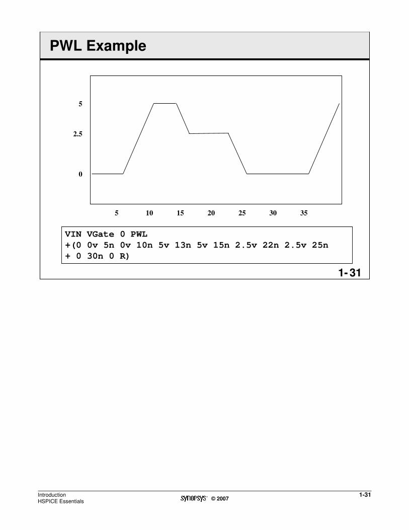
VIN VGate 0 PWL
+(0 0v 5n 0v 10n 5v 13n 5v 15n 2.5v 22n 2.5v 25n
+ 0 30n 0 R)
5 10 15 20 25 30 35
0
5
PWL Example
2.5

IntroductionHSPICE Essentials
1-32© 2007
321-
Independent Transient Sources: PAT
� Pattern Source
PAT <(> vhi vlo td tr tf tsample data
+ <RB=val> <R=repeat> <)>
� Uses four states
� '1‘ – high
� '0‘ – low
� 'm‘ – middle
� 'z' – high impedance
� The series of these four states is called a “bstring”
Examples:
V1 1 0 PAT (5 0 0n 1n 1n 5n b1011 rb=2)
VIN 1 0 PAT (2 0 40p 20p 80p 400p b1010110 r=1)

IntroductionHSPICE Essentials
1-33© 2007
331-
Independent Transient Sources: PRBS
� Pseudo Random Bit Generator Source
LFSR <(> vlow vhigh tdelay trise tfall rate
+ seed <[> taps <]> <rout=val> <)>
� seed is the initial value loaded into the shift register
� taps are the bits used to generate feedback
Example:
vin in gnd LFSR (0 1 1m 1n 1n 10meg 1 [5, 2] rout=10)

IntroductionHSPICE Essentials
1-34© 2007
341-
Independent Transient Sources: SIN
� SIN
� Syntax:
SIN vo va <frequency <tdelay <damping
+ <phasedelay>>>>
Example:
VIN 3 0 SIN (0 1 100MEG 1ns 1e10)
� Damped sinusoidal source
� Connected between nodes 3 and 0
� Offset of 0v
� Peak amplitude of 1v
� Frequency of 100 MHz
� Time delay of 1ns
� Damping factor of 1e10
� Phase delay of 0 degrees (default)

IntroductionHSPICE Essentials
1-35© 2007
351-
Mixed Independent Sources
� Mixed (composite) sources
� Specify source values for more than one type of analysis
� Depending on the analysis performed, the associated analysis sources are used
� Zero time value of transient source overrides the value of the DC source when transient operating point is calculated
Examples:VH 3 6 DC=2 AC=1,90
VCC 10 0 VCC PWL 0 0 10n VCC 15n VCC 20n 0
VIN 13 2 0.001 AC 1 SIN (0 1 1Meg)

IntroductionHSPICE Essentials
1-36© 2007
361-
Dependent Sources (1/3)
� Controlled Elements:
� High-level of abstraction
� Used for behavioral modeling and to simplify circuit descriptions
� Faster execution time
� Based on an arbitrary algebraic equation as the transfer function for a voltage or current source
� Common method used to create function libraries of subcircuits containing behavioral elements
� Types:
� G -- Voltage and/or current controlled current source
� E -- Voltage and/or current controlled voltage source
� H -- Current controlled voltage source
� F -- Current controlled current source

IntroductionHSPICE Essentials
1-37© 2007
371-
Dependent Sources (2/3)
� G and E sources can have several forms:
� Voltage Controlled Resistor and Capacitor
� Linear
� Polynomial
� PWL
� Multi-Input Gates
� Delay Element
� G and E sources are recommended over H and F sources

IntroductionHSPICE Essentials
1-38© 2007
381-
Dependent Sources (3/3)
� With dependent sources you can model:
� AND, NAND, OR, NOR gates
� MOS, bipolar transistors
� OP amps, summers, comparators
� Switched capacitor circuits, etc.
� Switches (using VCR)
� Syntax:
� Linear
� Exxx n+ n- <VCVS> in+ in- gain <options>
� Polynomial
� Exxx n+n- <VCVS>POLY(NDIM) in1+in1- …
+ inndim+ inndim- <options>

IntroductionHSPICE Essentials
1-39© 2007
391-
Dependent Source Examples
� Linear:
Egain 3 0 Vp Vn 1E3
V(3,0) = V(p,n)*1000
� Polynomial:
E1 1 0 POLY(2) 3 2 7 6 0 3 0 0 0 4
+FV=P0+P1*FA+P2*FB+P3*FA^2+P4⋅FA⋅FB+P5*FB2^2
+P6*FA^3+P7*FA^2*FB+P8*FA*FB^2+P9*FB^3+…
V (1,0) = 3 * V(3,2) + 4 * V(7,6)^2

IntroductionHSPICE Essentials
1-40© 2007
401-
Discovery AMS Simulation Interface Basics
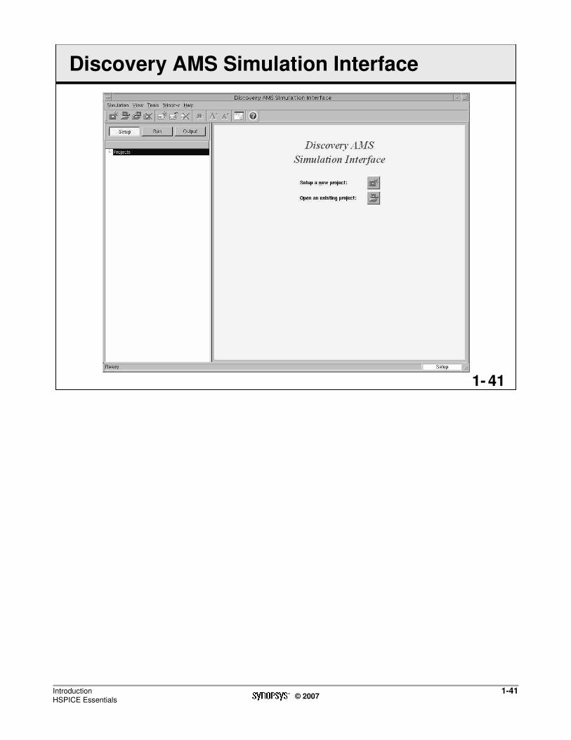
� To start the Discovery AMS Simulation Interface
% simif
� Setup a new project
� Project name
� New directory for all project test benches
� Project location
� Location of project directory
� Open an existing project
IntroductionHSPICE Essentials
1-41© 2007
411-
Discovery AMS Simulation Interface

IntroductionHSPICE Essentials
1-42© 2007
421-
Discovery AMS Simulation Interface – Project Management
� Manage the project test benches
� Close the project
� Delete the project
� Create a new test
� Import an older simulation (.wrk) file

IntroductionHSPICE Essentials
1-43© 2007
431-
Discovery AMS Simulation Interface – Project Management

IntroductionHSPICE Essentials
1-44© 2007
441-
Discovery AMS Simulation Interface – Setup
� HSPICE simulation is divided into 3 major tasks
� Setup
� Netlist and Simulation
� HSPICE Setup
� Run
� Output
� Selected by buttons near the top, left of the workbench
� Each button selects a new set of screens
� The GUI always starts in the Setup mode
� Each task contains either tabs or buttons that allow the user to enter specific information and data required by HSPICE

IntroductionHSPICE Essentials
1-45© 2007
451-
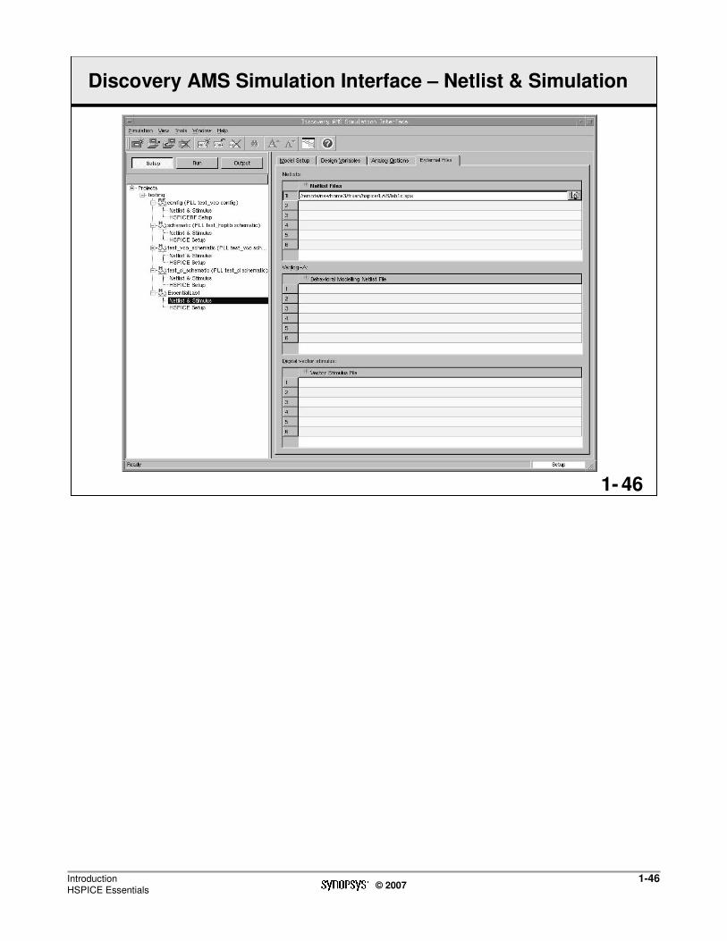
Discovery AMS Simulation Interface – Netlist & Simulation
� Netlist & Simulation is select from the tree on the left of the GUI
� Model Setup
� Name and corner of any model files used by the design
� Design Variables
� Design parameters
� Analog Options
� Set SCALE and TNOM options
� External Files
� Specify the netlist file(s) used by the design
� Specify the Verilog-A behavioral model files by the design
� Specify the name of any vector file(s) used by the design
IntroductionHSPICE Essentials
1-46© 2007
461-
Discovery AMS Simulation Interface – Netlist & Simulation

IntroductionHSPICE Essentials
1-47© 2007
471-
Discovery AMS Simulation Interface – HSPICE Setup
� Analysis
� Supports all HSPICE analyses
� Waveform
� Output waveforms setup� supports both .PROBE and .PRINT
� Select waveform viewer� Cosmos Scope (default)
� AvanWaves
� Post Proc
� Setups for .MEAS, .STIM and .BIASCHK statements
� Convergence
� .IC and .NODESET setup
� .SAVE and .LOAD
� Options
� Frequently used HSPICE options in its own category
� Commands
� Setup any options or commands not available from the setup screens
� Behavioral
� Verilog-A

IntroductionHSPICE Essentials
1-48© 2007
481-
Discovery AMS Simulation Interface – HSPICE Setup

IntroductionHSPICE Essentials
1-49© 2007
491-
Discovery AMS Simulation Interface – Run
� Run any simulation that is setup
� View listing (.lis) file
� Errors and warnings are highlighted
� View run script and header file
� Start waveform viewer
� CosmosScope

IntroductionHSPICE Essentials
1-50© 2007
501-
Discovery AMS Simulation Interface – Run

IntroductionHSPICE Essentials
1-51© 2007
511-
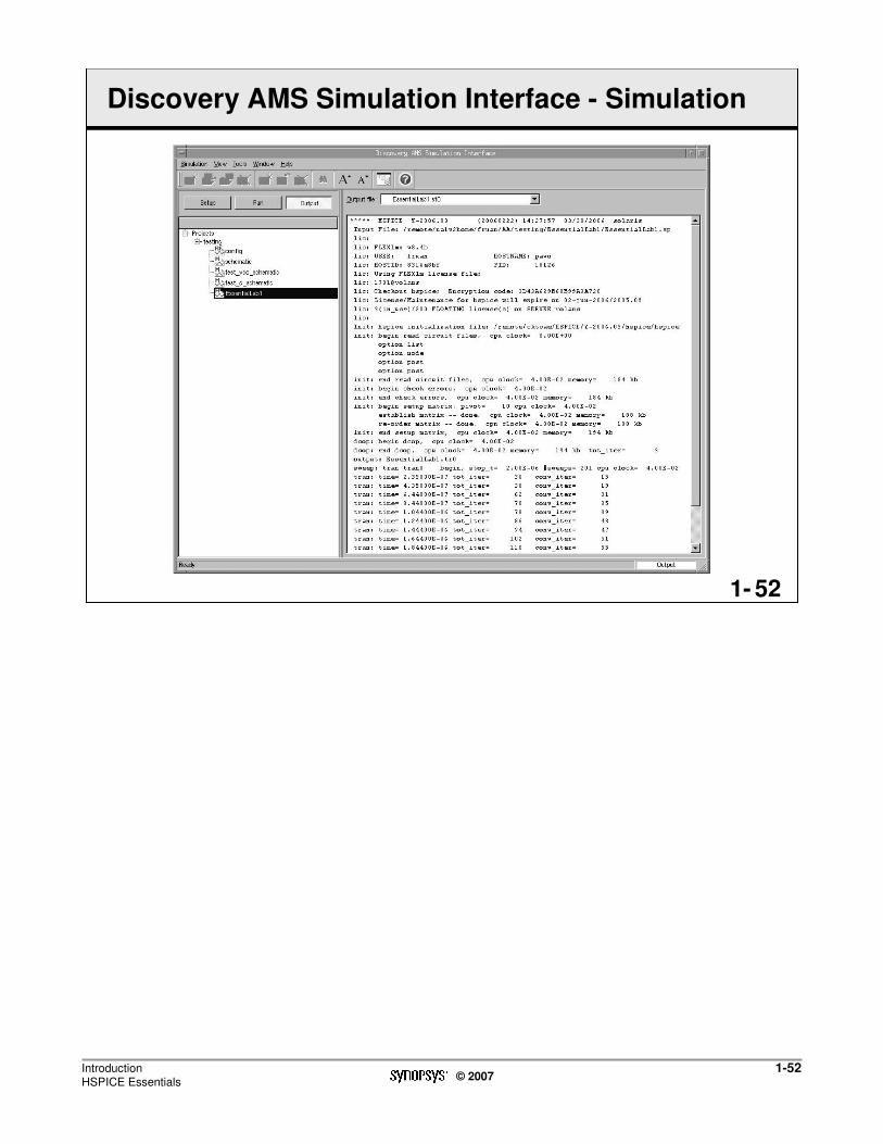
Discovery AMS Simulation Interface - Output
� View Status file (*.st#)
� View Subcircuit cross-listing (*.pa#)
� View Initial condition (*.ic#)
� View .MEASURE results
� AC measures (*.ma#)
� DC measures (*.ms#)
� Transient measures (*.mt#)
� .MEASURE file processing
IntroductionHSPICE Essentials
1-52© 2007
521-
Discovery AMS Simulation Interface - Simulation

IntroductionHSPICE Essentials
1-53© 2007
531-
Invoking CosmosScope
� UNIX/Linux Users
� Type cscope at the command prompt:
% cscope
� Windows Users:
� Select Start>Programs>Synopsys>2005.09>Cosmos-Scope>CosmosScope
IntroductionHSPICE Essentials
1-54© 2007
541-
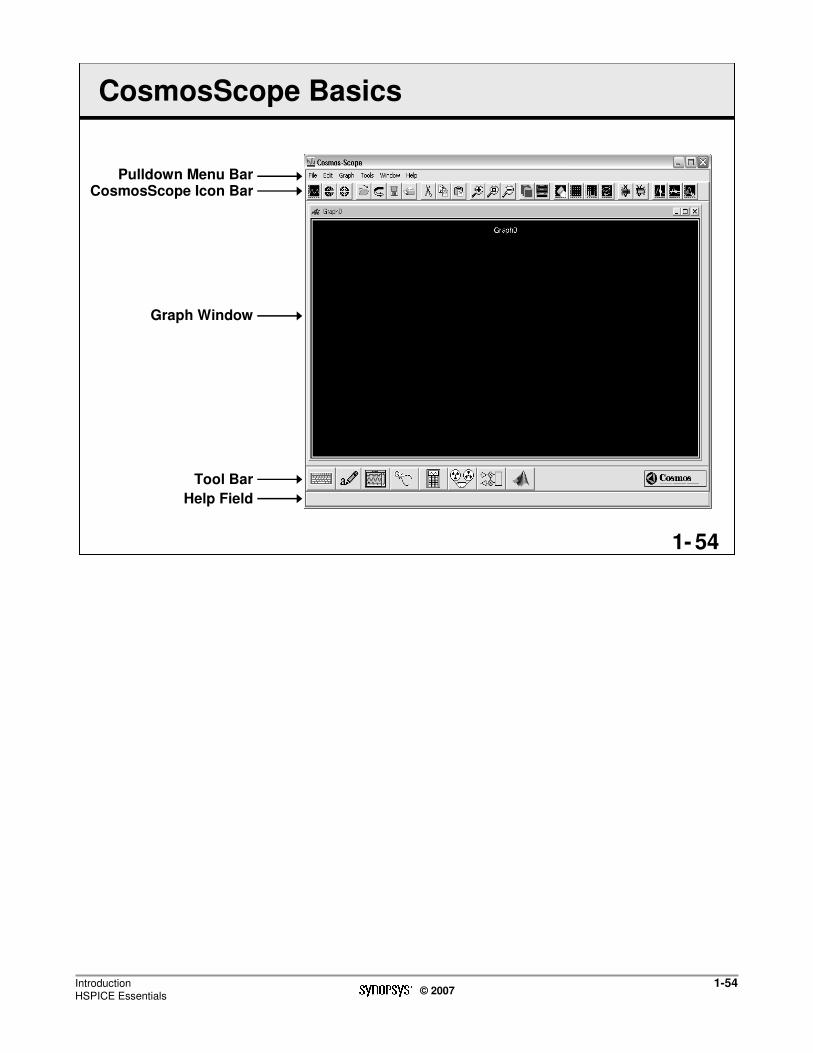
CosmosScope Basics
Pulldown Menu BarCosmosScope Icon Bar
Graph Window
Tool Bar
Help Field

IntroductionHSPICE Essentials
1-55© 2007
551-
CosmosScope Pulldown Menu Bar
Edit/Preferences
Graph/Plot
File Control
Graph Window
Control
Alternate Tool Bar
Icon Control
CosmosScope
Window Control
CosmosScope
Help

IntroductionHSPICE Essentials
1-56© 2007
561-
CosmosScope Icon Bar
New XY
Graph
New Smith
Chart
New Polar
Chart
Open
Reload
Save
Cut
Copy
Paste
Zoom
In
Zoom
to Fit
Zoom
Out
Cascade
Windows
Tile
Windows
Toggle
Grid
Toggle
Signal Grid
Configure
Dynamic
Waveform Display
Create
Bus
Burst
Bus
At X
Meas.
At Y
Meas.
Point to
Point Meas.
Clear

IntroductionHSPICE Essentials
1-57© 2007
571-
CosmosScope Tool Bar
Drawing Tool
AIM Command
LineSignal Manager
Measurement
Tool
Waveform
CalculatorMacro
Recorder
RF Tool
Matlab
Command
Line

IntroductionHSPICE Essentials
1-58© 2007
581-
CosmosScope Mouse Usage
� Left-click to select (buttons, objects, etc.)
� Right-click on anything to get a context-sensitive menu
� Middle-click to paste what is selected in the pointed-to location
� Drag with the middle button held down for panning
� For a two-button mouse, middle-click can be emulated by clicking the right and left mouse buttons simultaneously
� Shift-click the left mouse button to add to your selection if working with graphical objects; in list boxes, shift-click adds everything from your current selection to the click point
� Control-click the left mouse button to add to your selection
� Drag with the left mouse button held down to zoom (expand) the contents inside the box

IntroductionHSPICE Essentials
1-59© 2007
591-
Opening a Plotfile
� In the Scope Window
select File >Open > Plotfiles or click
the button
� Navigate to the directory where the
desired plotfile is located
� In the Files of type field, select the type of plotfile you would
like to open
� Select the plotfile and
click

IntroductionHSPICE Essentials
1-60© 2007
601-
CosmosScope File/Signal Control Forms
PlotfileManager
SignalManager
Graphic liberality

IntroductionHSPICE Essentials
1-61© 2007
611-
Scope Plotting Techniques (1/2)
� Plot one signal at a time:
� Method 1
� Left click the signal name in the signal manager
� Click the plot button
� Method 2
� Double-click the signal name
� Plot multiple consecutive signals:
� Method 1
� Click on the first signal
� Hold and drag to the last signal
� Click the plot button
� Method 2
� Click on the first signal and release
� Hold down the shift key and click on the last desired signal
� Click the plot button

IntroductionHSPICE Essentials
1-62© 2007
621-
Scope Plotting Techniques (2/2)
� Plot multiple non-consecutive signals:
� Click on the first signal
� Hold down the control key while clicking on other signals
� Then click the plot button
� Plot signals overlaying each other:
� Plot the first signal using any of the above approaches
� Select the signal to plot on top of the first signal
� Middle-click in the region of the first signal

IntroductionHSPICE Essentials
1-63© 2007
631-
CosmosScope Measurements
� Measurements are the the key to design analysis
� Over 50 built-in measurements at your fingertips
� Can be applied graphically in CosmosScope or in "Batch" mode for automatic data collection
� You can add custom measurements

IntroductionHSPICE Essentials
1-64© 2007
641-
CosmosScope Measurements

IntroductionHSPICE Essentials
1-65© 2007
651-
CosmosScope Measurements
� General Measurements:
� At X, at Y, delta X, delta Y, length, slope, local min/max, crossing, horiz. level, vert. level, vert. cursor, point marker, point to point
� Time Domain:
� Duty cycle, frequency, period, pulsewidth, risetime, falltime, slew rate, delay, overshoot, undershoot, settle time, eye diagram
� Reference or level measurements:
� Max, min, X at max, X at min, peak to peak, topline, baseline, amplitude, average, RMS, AC-coupled RMS
� Frequency Domain:
� Lowpass, highpass, bandpass (Q, ripple, etc.), stopband, phase margin, gain margin, slope, magnitude, dB, phase, real, imaginary, Nyquist plot frequency
� S Domain
� Damping ratio, natural frequency, quality factor
� Statistics:
� Max, min, range, mean, median, std. deviation, mean (+/- 3 std dev), histogram, yield, Dpu, Cpk, pareto

IntroductionHSPICE Essentials
1-66© 2007
661-
CosmosScope Calculator
Entry Field (Register)
Icon Bar
Pulldown Menus
Programmable Buttons
Stack Display
Extended Operation Buttons
Keypad

IntroductionHSPICE Essentials
1-67© 2007
671-
Using the Calculator
� To get a waveform into the Register:
� Select the waveform name on the graph window (or in the Plot File Window)
� Middle-click in the Register
� You can also select Edit > Paste in the calculator to accomplish this task
� Select either input mode: Reverse Polish Notation (RPN) or Algebraic
� To plot results from the calculator:
� Click the left-most icon in the Icon Bar

IntroductionHSPICE Essentials
1-68© 2007
681-
Lab 1: HSPICE
During this lab, you will:
1. Create a HSPICE netlist
2. Use the Discovery AMS Simulation Interface to set up and start HSPICE to simulate the netlist
3. View the results in CosmosScope
Netlist
Setup
Simulation
CosmosScope
90 minutes
Active Devices / AnalysisHSPICE Essentials
2-1© 2007
12-
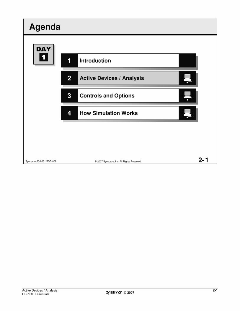
Agenda
© 2007 Synopsys, Inc. All Rights ReservedSynopsys 60-I-031-BSG-008
DAY
1111Introduction1
Active Devices / Analysis2
Controls and Options3
How Simulation Works4

Active Devices / AnalysisHSPICE Essentials
2-2© 2007
22-
Unit Objectives
After completing this unit, you should be able to:
� Use active devices and subcircuits in a netlist
� Use Verilog-A models
� Set up each analysis type
� Output the simulation results

Active Devices / AnalysisHSPICE Essentials
2-3© 2007
32-
Active Devices and Analysis Types
� Components:
� Active devices defined by element statements and models
� D - Diodes
� M - MOS Transistors
� Q - BJTs
� J - JFETs and MESFETs
� Subcircuits and Verilog-A modules
� Analysis Types:
� DC Operating Point
� DC Analysis
� AC Analysis
� Transient Analysis
� Temperature Analysis

Active Devices / AnalysisHSPICE Essentials
2-4© 2007
42-
Components: Diodes (1/2)
� D – Diodes
� Element Syntax:
Dxxx nplus nminus mname <options>
Example:
D1 3 0 DMOD IC=0.2v
Voltage of 0.2v at time 0
Diode model parameters contained in a model statement, DMOD

Active Devices / AnalysisHSPICE Essentials
2-5© 2007
52-
Components: Diodes (2/2)
� Model Syntax:
� .MODEL mname D <LEVEL=val> <keyname=val> …
Example:
.MODEL DMOD D (is=1e-14 rs=0.1 cjo=2pf)
� Three types of models:
� Level=1, Non-geometric - discrete (standard and Zener)
� Level=2, Fowler-Nordheim - nonvolatile EEPROM memory
� Level=3, Geometric - ic based standard Si diffused diodes

Active Devices / AnalysisHSPICE Essentials
2-6© 2007
62-
Components: MOS Transistor
� M - MOSFET
� Element Syntax:
Mxxx nd ng ns <nb> mname <L=val> <W=val>+ <options...>
Mxxx nd ng ns <nb> mname lval wval …
Examples:
M1 3 4 5 0 nch 5u 10u
M31 2 17 6 10 MODM l=5u w=2u
Mabc 2 9 3 0 mymod l=10u w=5u
+ ad=100p as=100p pd=40u ps=40u
� SCALING:
� Default units of length and width are METERS!
� Units are controlled by .OPTION SCALE and MODEL parameter SCALM

Active Devices / AnalysisHSPICE Essentials
2-7© 2007
72-
Components: MOS Transistor Model
� Model Syntax:
.MODEL mname PMOS (<level=val>
+ <keyname1=val1>...)
.MODEL mname NMOS (<level=val>
+ <keyname1=val1>...)
Examples:
.MODEL MODP PMOS (level=3 vto=-3.25 gamma=1.0)
.MODEL MODN NMOS (level=2 vto=1.85
+ tox=735e-10)
.MODEL nchan.1 nmos level=2 vto=2.0 uo=800
+ tox=500 nsub=1e15 rd=10 rs=10 capop=5

Active Devices / AnalysisHSPICE Essentials
2-8© 2007
82-
Components: JFET/MESFET
� J – JFET/MESFET
� Element Syntax:
Jxxx nd ng ns <nb> mname <W=val> <L=val>
+ <options>
Examples:
J1 7 2 3 JM1
jmes xload gdrive common jmodel
� SCALING:
� Default units of length and width are METERS!
� Units are controlled by .OPTION SCALE and MODEL parameter SCALM

Active Devices / AnalysisHSPICE Essentials
2-9© 2007
92-
Components: JFET/MESFET Model
� Model Syntax:
.MODEL mname NJF (<level=val>
+ <pname1=val1>...)
.MODEL mname PJF (<level=val>
+<pname1=val1>...)
Example:
.MODEL nj_acmo njf level=3
+ capop=1 sat=3 acm=0
+ is=1e-14 cgs=1e-15 cgd=.3e-15
+ rs=100 rd=100 rg=5 nd=1
Active Devices / AnalysisHSPICE Essentials
2-10© 2007
102-
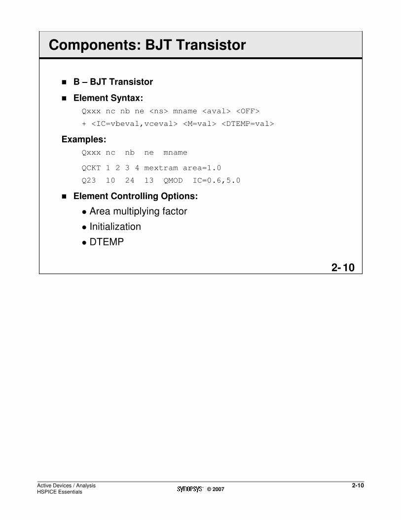
Components: BJT Transistor
� B – BJT Transistor
� Element Syntax:
Qxxx nc nb ne <ns> mname <aval> <OFF>
+ <IC=vbeval,vceval> <M=val> <DTEMP=val>
Examples:
Qxxx nc nb ne mname
QCKT 1 2 3 4 mextram area=1.0
Q23 10 24 13 QMOD IC=0.6,5.0
� Element Controlling Options:
� Area multiplying factor
� Initialization
� DTEMP

Active Devices / AnalysisHSPICE Essentials
2-11© 2007
112-
BJT Transistor Model
� MODEL Syntax:
.MODEL mname NPN <pname1=val1>…
.MODEL mname PNP <pname1=val1>…
Example:
.MODEL QMOD NPN ISS = 0 XTF=1 NS=1.0 CJS=0

Active Devices / AnalysisHSPICE Essentials
2-12© 2007
122-
Components: Subcircuits
� Subcircuit definition syntax:
.SUBCKT subnam n1 <n2 n3 …><parnam=val …>
� subnam – Reference name for the subcircuit model call
� n1, n2 … - Node numbers for external reference
� Any element nodes appearing in the subcircuit, but not included in this list, are strictly local, EXCEPT
� Ground node (0)
� Nodes assigned using BULK (MOSFET) or SUBSTRATE (BJT)
� Nodes assigned using the .GLOBAL statement
� parnam=val - A parameter name set to a value
� For use only in the subcircuit
� Overridden by an assignment in the subcircuit call or by a valueset in a .PARAM statement that is external to the subcircuit

Active Devices / AnalysisHSPICE Essentials
2-13© 2007
132-
Components: Subcircuit Calls
� X Element Syntax:
Xyyy n1 <n2 n3 …> subnam <parnam=val …>
+ <M=val>
� ALL subcircuit names begin with an X
Examples:
Xnand1 in1_1 in2_1 clk out_1 nand3
+ wn=10 ln=1
� Calls subckt named “nand3”
� Assigns parameters WN=10 and LN=1
– parameters WN and LN within the .SUBCKTXinv1 in out inv
� Calls subckt named “inv”
Active Devices / AnalysisHSPICE Essentials
2-14© 2007
142-
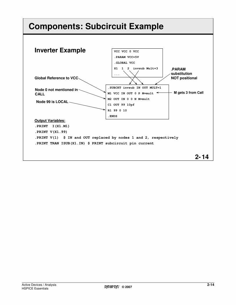
Components: Subcircuit Example
Inverter Example
Output Variables:
.PRINT I(X1.M1)
.PRINT V(X1.99)
.PRINT V(1) $ IN and OUT replaced by nodes 1 and 2, respectively
.PRINT TRAN ISUB(X1.IN) $ PRINT subcircuit pin current
M gets 3 from Call
VCC VCC 0 VCC
.PARAM VCC=5V
.GLOBAL VCC
X1 1 2 invsub Mult=3
...
.SUBCKT invsub IN OUT MULT=1
M1 VCC IN OUT 0 P M=mult
M2 OUT IN 0 0 N M=mult
C1 OUT 99 10pf
R1 99 0 10
.ENDS
Global Reference to VCC
Node 0 not mentioned in CALL
Node 99 is LOCAL
.PARAM substitution NOT positional

Active Devices / AnalysisHSPICE Essentials
2-15© 2007
152-
Global Statement
� .GLOBAL:
� Syntax
.GLOBAL node1 node2 node3 …
.GLOBAL VBIAS VCC
� Usage� When subcircuits are included in the data file
� Assigns common node name to subcircuit nodes
� Power supply connection of all subcircuits often done this way
.GLOBAL VCC
– Connects all nodes named VCC, including subcircuits with the internal node named VCC
Note:
� Do not specify power pins in subcircuit calls
� Use .GLOBAL VCC
Active Devices / AnalysisHSPICE Essentials
2-16© 2007
162-
Introduction to Verilog-A
� What is Verilog-A
� Standard analog hardware description language
� The analog-only subset of Verilog-AMS
� Verilog-AMS LRM, version 2.2, released in November 2004
� Verilog-A applications
� Multi-level design simulation
� Compact models
� Analog test benches
� Verilog-A in HSPICE
� Compiled Verilog-A Solution
� Single kernel simulation

Active Devices / AnalysisHSPICE Essentials
2-17© 2007
172-
Feature Overview
� Industry standard compliant Verilog-A language support
� Compatible with Verilog-AMS LRM 2.2
� Users should be able to use existing Verilog-A code without changes
� HSPICE Verilog-A device are supported with existing syntax
� Verilog-A modules are instantiated in the same manner as HSPICE subcircuits
� Features available on HSPICE will be supported in Verilog-A based devices
� Users do not lose any significant simulator functionality with Verilog-A based devices

Active Devices / AnalysisHSPICE Essentials
2-18© 2007
182-
Verilog-A Usage Overview
� Verilog-A modules are loaded into the system via “.hdl”command
� Modules are instantiated with the same syntax as HSPICE subcircuits
� Verilog-A device data can be output using conventional output commands
•Simple Verilog-A amplifier
.hdl my_amp.va
vs 1 0 1
rs 1 0 1
x1 1 2 my_amp gain=10
rl 2 0 1
.print tran V(x1.in) I(x1.out) x1:gain
module my_amp(in, out);
electrical in, out;
parameter real gain = 1.0;
analog begin
V(out) <+ gain * V(in);
end
endmodule

Active Devices / AnalysisHSPICE Essentials
2-19© 2007
192-
Loading Verilog-A Files
� Two ways to load Verilog-A files
� .hdl netlist command
� Follows the syntax of NanoSim
Example:
.hdl “my_amp.va”
� -hdl command line option
� Allows simulations to choose whether Verilog-A modules are used or not
� Verilog-A modules can be changed without netlist modification
Example:
hspice test.sp –hdl pll.va –vamodel –o test
� The Verilog-A file is assumed to have the .va extension when only prefix is supplied

Active Devices / AnalysisHSPICE Essentials
2-20© 2007
202-
Instantiation Syntax
� Verilog-A devices are X devices in HSPICE netlist
� SyntaxX<inst> <nodes>* moduleName|modelName <param=value>*
Example:Xva_r plus minus va_r res=100
� Verilog-A module may be instantiated directly or instantiated via an associated Verilog-A model card

Active Devices / AnalysisHSPICE Essentials
2-21© 2007
212-
Verilog-A Model Cards
� Model card is a parameter sharing mechanism
� When parameter sets are almost the same they can be shared among many instances
� Advantage to compact model
� Syntax is the same for Verilog-A devices as for built-in devices
� Verilog-A model syntax
.model modelName modelType param=value
modelType - Verilog-A module name, cannot conflict with built-in model types (e.g., R, C, D, etc.)
modelName - model name reference used by the instance
Example:
.model my_bjt_va bjt_va rb=6.5 rc=6.3 re=0.15

Active Devices / AnalysisHSPICE Essentials
2-22© 2007
222-
Instantiation Examples (1/2)
// Verilog-A module example
module va_amp(in, out);
electrical in,out;
parameter real gain=1.0, fc=100e6;
analog begin
…
endmodule
** Associate model cards of va_amp can be:
. model myamp va_amp gain=2 fc=200e6
. model myamp2 va_amp gain=10

Active Devices / AnalysisHSPICE Essentials
2-23© 2007
232-
Instantiation Examples (2/2)
** Instantiations of Verilog-A module ‘va_amp’
x1 n1 n2 myamp
x2 n3 n4 myamp gain=2.0
x3 n5 n6 myamp2 fc=150e6
x4 n7 n8 va_amp
� x1 inherits model ‘myamp’ parameters gain=2, fc=200e6
� x2 inherits ‘fc=200e6’ from ‘myamp’ and overrides ‘gain’
� x3 inherits parameter “gain=10” from model ‘myamp2’ and overrides parameter ‘fc’ which is an implicit parameter in ‘myamp2’
� x4 directly instantiates the Verilog-A module ‘va_amp’

Active Devices / AnalysisHSPICE Essentials
2-24© 2007
242-
Parameter Case Sensitivity
� Verilog-A is case sensitive
� HSPICE is case insensitive
� Module parameters that differ by case only cannot be redefined in its netlist instantiations
Example:
module my_amp(in, out);
electrical in, out;
parameter real gain = 1.0;
parameter real Gain = 1.0;
analog V(out) <+ (Gain+gain)*V(in);
endmodule
� If the user instantiates the module as:
x1 n1 n2 my_amp Gain=1
� The simulator cannot uniquely define which parameter is to be set
� A warning message regarding the ambiguity is issued and the definition of the parameter is ignored

Active Devices / AnalysisHSPICE Essentials
2-25© 2007
252-
Output Control
� Output for Verilog-A devices:
� Direct port voltage access
� Direct port current probing
� Internal node voltage access
� Internal named branch probing
� Module parameter value
� Module variable value

Active Devices / AnalysisHSPICE Essentials
2-26© 2007
262-
Output Control Examples
� To print the current on Verilog-A device port name plus for the instance x1:
.print I(x1.plus)
� To print the Verilog-A module internal node named int1 for the instance x1:
.print V(x1.int1)
� In this module there is an internal branch name br1 declared, then the branch current can be probed as:
.print I(x1.br1)
� If the module va_fnc is hierarchical and has a child instance called c1 with an internal node c_int1 then the node c_int1 can be output as:
.print V(x1.c1.c_int1)

Active Devices / AnalysisHSPICE Essentials
2-27© 2007
272-
Verilog-A Examples
Examples of typical Verilog-A modules with HSPICE netlists are located at:
$installdir/demo/hspice/veriloga/

Active Devices / AnalysisHSPICE Essentials
2-28© 2007
282-
Analysis Types: Types and Order
� Types and Order of Execution:
� DC Operating Point
� First and most important job is to determine the DC steady stateresponse (called the DC operating point)
� DC Bias Point and DC Sweep Analysis
� .DC, .OP, .TF, .SENS
� AC Bias Point and AC Frequency Sweep Analysis
� .AC, .LIN, .NET, .NOISE, .DISTO
� Transient Bias Point and Transient Sweep Analysis
� .TRAN, .FFT, .Fourier, .OP <time>
� Temperature Analysis
� .TEMP
� Advanced Modifiers: Monte Carlo, Optimization, Variability

Active Devices / AnalysisHSPICE Essentials
2-29© 2007
292-
Analysis Types: DC Operating Point (1/2)
� Syntax
.OP <format> <time> <format> <time>
� format – all, current, voltage, brief, debug or none
� Default is all
� time – specifies the time at which HSPICE prints the report
� Default is time=0
� The DC Operating Point (bias point) is calculated first for ALL analysis types:
� Caps OPEN
� Inductors SHORT
� Initialized by .IC, .NODESET, and voltage sources at their time=0 values
� For Transient analysis, the operating point can be disabled with the UIC option in the .TRAN statement

Active Devices / AnalysisHSPICE Essentials
2-30© 2007
302-
Analysis Types: DC Operating Point (2/2)
� Operating point analysis prints:
� Node voltages
� Source currents
� Power dissipation at the operating point
� Semiconductor device currents, conductances, capacitances
� Initialization:
� .NODESET
� Initial conditions released before final DC Operating Point
� .IC
� Initial conditions held and become part of the DC Operating Point Solution

Active Devices / AnalysisHSPICE Essentials
2-31© 2007
312-
Analysis Types: DC Analysis
� DC and Operating Point Analysis Statements:
� .DC Sweeps for power supply, temperature, parameter, transfer curves
� .PZ Pole/Zero Analysis
� .TF DC small-signal transfer function
� .DC Statement Sweeps:
� Any parameters
� Any source value
� Temperature
� DC Monte Carlo (random sweep)
� DC circuit optimization
� DC model characterization

Active Devices / AnalysisHSPICE Essentials
2-32© 2007
322-
Analysis Types: DC Analysis Syntax (1/2)
� Syntax:
.DC var1 start1 stop1 incr1+ <var2 start2 stop2 incr2>
.DC var1 start1 stop1 incr1+ <SWEEP var2 type np start2 stop2>
Examples:
.DC VIN 0.25 5.0 0.25
� Sweep VIN from .25 to 5v by .25v increments
.DC VDS 0 10 .5 VGS 0 5 1
� Sweep VDS from 0 to 10v by .5 incr at VGS values of 0, 1, 2, 3, 4 and, 5v
.DC TEMP -55 125 10
� Sweep TEMP from -55°C to 125°C in 10 degree increments

Active Devices / AnalysisHSPICE Essentials
2-33© 2007
332-
Analysis Types: DC Analysis Syntax (2/2)
Examples continued:
.DC xval 1k 10k 0.5k SWEEP TEMP LIN 5 25 125
� DC analysis performed at each temperature value
� Linear TEMP sweep from 25°C to 125°C (5 points) while sweeping a resistor value called ‘xval’ from 1K to 10K in 0.5K increments
.DC DcSrc START=0 STOP=srcval+ STEP=‘srcval/100’
� Parameterize start, stop, incr values
� Several Forms depending on the application:
� Single or double sweep
� Monte Carlo
� Parameterized Sweep
� Optimization

Active Devices / AnalysisHSPICE Essentials
2-34© 2007
342-
Analysis Types: AC Analysis
� AC Analysis:
� Compute output variables as a function of frequency
� Requires an AC source (v2 n1 n2 5 ac 1...)
� Set to 1 volt for normalized db plot
� First solves DC operating point
� Vary the frequency and observe the performance of the circuit
� .AC Statement Sweeps:
� Frequency
� Element value
� Temperature
� Model parameter value
� Random sweep (Monte Carlo)
� Optimization and AC design analysis

Active Devices / AnalysisHSPICE Essentials
2-35© 2007
352-
Analysis Types: AC Analysis Syntax
� Syntax:
.AC var1 start1 stop1 incr1+ <SWEEP var2 type np start2 stop2>
.AC type np fstart fstop+ <SWEEP var start stop incr>
� Examples:
.AC DEC 10 1K 100MEG
� Frequency sweep 10 points per decade from 1kHz to 100MHz
.AC LIN 100 1 100hz
� Linear sweep 100 points from 1Hz to 100Hz
.AC DEC 10 1 10K SWEEP cload LIN 20 1pf 10pf
� AC analysis for each value of cload, with a linear sweep of cload between 1pf and 10pf (20 points), sweeping frequency 10 points per decade from 1Hz to 10kHz
.AC DEC NPOINT=<expr> START=<expr> STOP=<expr>
� Must be ascending
� Parameterize np, start, stop values

Active Devices / AnalysisHSPICE Essentials
2-36© 2007
362-
Analysis Types: Other AC Analyses
� Other AC Analyses:
� .LIN Linear analysis
� .NOISE Noise analysis
� .LIN:
� Extracts multi-port [S, Y, Z, or H] parameters, group delay values and noise parameters for a general multi-port network
� .NOISE:
� Each noise source is calculated independently
� Total output noise voltage is the RMS sum of the individual noise contributions
� Can use .LIN to calculate noise

Active Devices / AnalysisHSPICE Essentials
2-37© 2007
372-
Analysis Types: Transient Analysis (1/3)
� Transient Analysis Statements:
� Calculate a DC operating point, the time=0 value of the circuit
� Compute circuit solution as a function of time
� The DC operating point is skipped if UIC is specified in the .tran statement
� .TRAN statement can be used for:
� Operating point (e.g., .OP 20n)
� Temperature sweep
� Monte Carlo analysis
� Parameter sweep
� Optimization
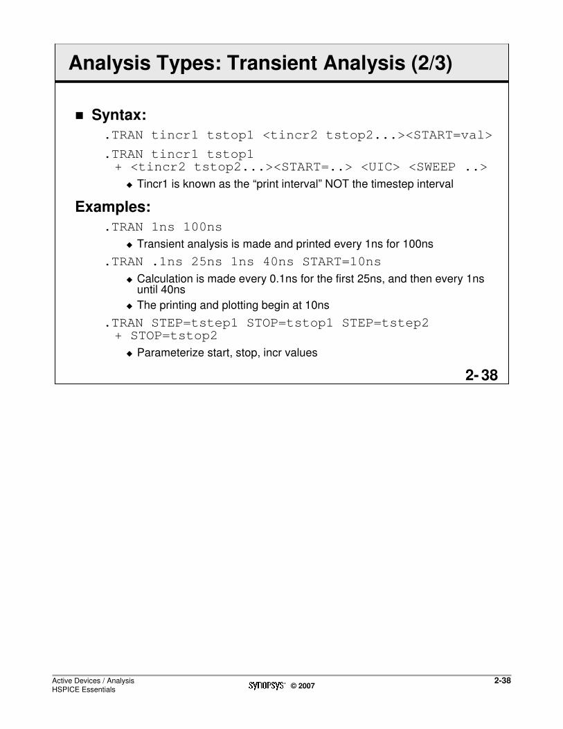
Active Devices / AnalysisHSPICE Essentials
2-38© 2007
382-
Analysis Types: Transient Analysis (2/3)
� Syntax:
.TRAN tincr1 tstop1 <tincr2 tstop2...><START=val>
.TRAN tincr1 tstop1+ <tincr2 tstop2...><START=..> <UIC> <SWEEP ..>
� Tincr1 is known as the “print interval” NOT the timestep interval
Examples:
.TRAN 1ns 100ns
� Transient analysis is made and printed every 1ns for 100ns
.TRAN .1ns 25ns 1ns 40ns START=10ns
� Calculation is made every 0.1ns for the first 25ns, and then every 1ns until 40ns
� The printing and plotting begin at 10ns
.TRAN STEP=tstep1 STOP=tstop1 STEP=tstep2+ STOP=tstop2
� Parameterize start, stop, incr values

Active Devices / AnalysisHSPICE Essentials
2-39© 2007
392-
Analysis Types: Transient Analysis (3/3)
Examples:
.TRAN 10ns 1us SWEEP cload POI 3 1pf 5pf 10pf
� Analysis will be performed for each cload value (1pf, 5pf and 10pf)
� Keyword POI - Points of Interest
� Several Forms depending on the application:
� Single or double sweep
� Random Monte Carlo
� Parameterized Sweep
� Optimization

Active Devices / AnalysisHSPICE Essentials
2-40© 2007
402-
Analysis Types: Other Transient Analyses
� Other Transient Analyses:
� .FOUR
� Fourier decomposition analysis
� Performed on 501 points of transient analysis date of the last 1/f time period
� Output is DC component and first 9 harmonics
� .FFT
� Fast Fourier Transform
� Uses internal time point values
� By default the entire waveform is analyzed
– Can set start and stop times
� Can specify windowing functions
– Reduce spectral leakage
� Default number of waveform points is 1024
– Can be set by user but, must be a power of 2
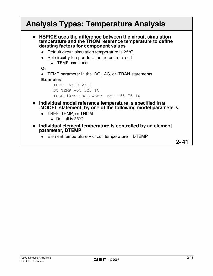
Active Devices / AnalysisHSPICE Essentials
2-41© 2007
412-
Analysis Types: Temperature Analysis
� HSPICE uses the difference between the circuit simulation temperature and the TNOM reference temperature to define derating factors for component values
� Default circuit simulation temperature is 25°C
� Set circuitry temperature for the entire circuit� .TEMP command
Or
� TEMP parameter in the .DC, .AC, or .TRAN statements
Examples:
.TEMP -55.0 25.0
.DC TEMP -55 125 10
.TRAN 10NS 1US SWEEP TEMP -55 75 10
� Individual model reference temperature is specified in a .MODEL statement, by one of the following model parameters:
� TREF, TEMP, or TNOM� Default is 25°C
� Individual element temperature is controlled by an element parameter, DTEMP
� Element temperature = circuit temperature + DTEMP

Active Devices / AnalysisHSPICE Essentials
2-42© 2007
422-
Analysis Types: Temperature Analysis Example
.TEMP 100
D1 N1 N2 DMOD DTEMP=30
D2 NA NC DMOD
.MODEL DMOD D IS=1E-15 VJ=0.6 CJA=1.2E-13
+ CJP=1.3E-14 TREF=60.0
� Circuit simulation temperature is 100°C (.TEMP)
� Element Temperature for D1 = 100°C + 30°C = 130°C
� Element Temperature for D2 = 100°C
� Diode model statement specifies TREF at 60°C
� The derating of the model parameters is based on the difference between circuit simulator temperature and TREF
� Model derating factor for D1 = 70°C (130°C - 60°C)
� Model derating factor for D2 = 40°C (100°C - 60°C)

Active Devices / AnalysisHSPICE Essentials
2-43© 2007
432-
Output and Formatting
� Output Commands
� Output Variables

Active Devices / AnalysisHSPICE Essentials
2-44© 2007
442-
Output Commands (1/2)
� Output Commands:
� .PROBE
� .MEASURE
� Each statement specifies:
� Output variable
� Simulation result to be displayed

Active Devices / AnalysisHSPICE Essentials
2-45© 2007
452-
Output Commands (2/2)
� .PROBE:
� Save output variables in analysis data file without additional output in the output listing file
� With option probe, can limit *.TR# file size
� .PRINT:
� Numeric analysis results printed to output listing file
� .MEASURE:
� Print numeric results of measured electrical specifications for specified analysis
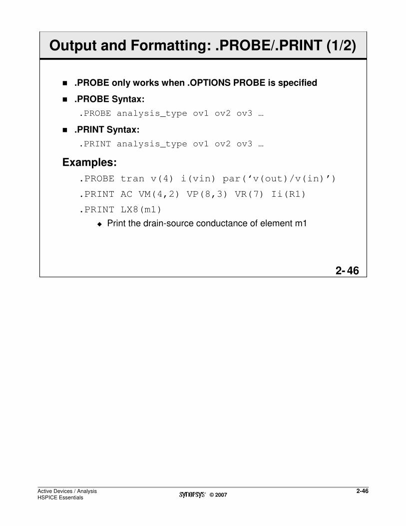
Active Devices / AnalysisHSPICE Essentials
2-46© 2007
462-
Output and Formatting: .PROBE/.PRINT (1/2)
� .PROBE only works when .OPTIONS PROBE is specified
� .PROBE Syntax:
.PROBE analysis_type ov1 ov2 ov3 …
� .PRINT Syntax:
.PRINT analysis_type ov1 ov2 ov3 …
Examples:
.PROBE tran v(4) i(vin) par(‘v(out)/v(in)’)
.PRINT AC VM(4,2) VP(8,3) VR(7) Ii(R1)
.PRINT LX8(m1)
� Print the drain-source conductance of element m1

Active Devices / AnalysisHSPICE Essentials
2-47© 2007
472-
Output and Formatting: .PROBE/.PRINT (2/2)
� When using .PROBE with Subcircuits (Xnnn):
� Specify nodes ‘local’ to a subcircuit
� Nodes on ‘calling’ line replace local nodes
� Concatenate circuit pathname with the node name through the ‘.’
X1.XBIAS.M5
� Based on unique number automatically assigned to each subcircuit (.OPTION LIST)
56:M5
� In this case, HSPICE assigned 56 to X1.XBIAS

Active Devices / AnalysisHSPICE Essentials
2-48© 2007
482-
Using .PROBE/.PRINT with Subcircuits
Subcircuit Example:
X1 1 2 INV
.subckt INV 36 34
m1 35 36 34 34 pp w=4u l=10u
m2 34 36 37 37 nn w=2u l=10u
R1 35 99 10K
R2 99 37 10K
R3 99 36 100K
.ends
.print DC v(2) I(X1.M2)
.print DC v(X1.99)
.option post probe

Active Devices / AnalysisHSPICE Essentials
2-49© 2007
492-
Output Format: Analysis Data (1/2)
� Specifying analysis data format:
� .OPTION POST
� Creates binary file
� Same as POST=1
� .OPTION POST=2
� Creates ASCII file
� Platform independent
� Limiting the size of the analysis data file:
� .OPTION PROBE
� ALL nodes plotted by default
� Limit data in analysis data file to that specified in .PRINT and .PROBE statements

Active Devices / AnalysisHSPICE Essentials
2-50© 2007
502-
Output Format: Analysis Data (2/2)
� Limiting the size of the analysis data file:
� .OPTION INTERP
� Limit the number of points stored to step size specified in .tran statement
� Pre-interpolates the output to the interval specified on the .TRAN statement
� Usually results in smaller graph data files
� .PROBE:
� Write directly to the analysis data file

Active Devices / AnalysisHSPICE Essentials
2-51© 2007
512-
Output Waveform Display
How to limit the size of the waveform files:
Netlist Input File, *.sp Waveform File, *.tr0
.option post All nodes and points
.option post probe Fewer nodes
.option post interp Fewer points per node

Active Devices / AnalysisHSPICE Essentials
2-52© 2007
522-
Output Variables
� Five Groups of Output Variables:
� DC and transient analysis
� Displays individual nodal voltages, branch currents, element power dissipation
� AC analysis
� Displays imaginary and real components of nodal voltage, branch current. Also phase, impedance parameters
� Element templates
� Displays element specific nodal voltages, branch currents, element parameters, and the derivatives of element voltage, current, or charge
� .MEASURE
� Displays user-defined variables as specified in the .MEASURE statement
� Parametric statements
� Displays mathematically, user-defined expressions operating on nodal voltages, etc

Active Devices / AnalysisHSPICE Essentials
2-53© 2007
532-
Output Variables: DC and Transient (1/2)
� DC and Transient output examples:
� Standard form is V(node) or I(element)
v(1)
� Voltage at node 1
i(Rin)
� Current through Rin (direction of I is n1 to n2)
v(1,2)
� Voltage between node 1 and node 2 (differential)
� Complex addressing
i1(xinv1.m3)
� Drain current of transistor m3 in subcircuit inv1

Active Devices / AnalysisHSPICE Essentials
2-54© 2007
542-
Output Variables: DC and Transient (2/2)
� DC and Transient output examples (cont.)
p(rload)
� Power dissipated in rload at point of analysis
p(m1)
� Power dissipated in transistor m1 at point of analysis
Power
� Total power dissipation output at point of analysis
v(x3.5)
� Voltage at INTERNAL node 5 of subckt x3
par(‘p(x1.m1)+p(x2.m2)’)
� Sum of power in m1 of x1 and m2 of x2
i3(2:q2)
� Emitter current of q2 in second subcircuit called

Active Devices / AnalysisHSPICE Essentials
2-55© 2007
552-
Output Variables: AC
� AC analysis output examples:
vi(2)
� Imaginary voltage component at node 2
ip1(q4)
� The phase of the collector current in q4
vdb(2,8)
� The voltage ratio between node 2 and 8 in decibels
vp(4,6)
� The arctangent [vi(4,6)/vr(4,6)]
vp(6)
� Phase at node 6

Active Devices / AnalysisHSPICE Essentials
2-56© 2007
562-
Using ACOUT Option (1/3)
� ACOUT controls the AC output calculation method, for the difference in values of magnitude, phase, and decibels:
� ACOUT = 1 (default) selects HSPICE method, which calculates the difference of the magnitudes of the values
� Real and imaginaryVR(N1,N2) = REAL [V(N1,0)] - REAL [V(N2,0)]
VI(N1,N2) = IMAG [V(N1,0)] - IMAG [V(N2,0)]
� MagnitudeVM(N1,0) = [VR(N1,0)2 + VI(N1,0)2]0.5
VM(N2,0) = [VR(N2,0)2 + VI(N2,0)2]0.5
VM(N1,N2) = VM(N1,0) - VM(N2,0)
� PhaseVP(N1,0) = ARCTAN[VI(N1,0)/VR(N1,0)]
VP(N2,0) = ARCTAN[VI(N2,0)/VR(N2,0)]
VP(N1,N2) = VP(N1,0) - VP(N2,0)
� Decibel
VDB(N1,N2) = 20 · LOG10(VM(N1,0)/VM(N2,0))
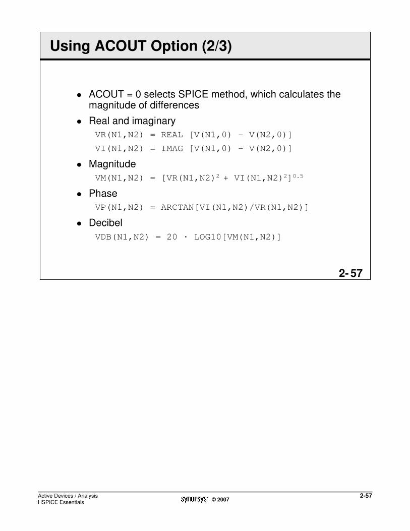
Active Devices / AnalysisHSPICE Essentials
2-57© 2007
572-
Using ACOUT Option (2/3)
� ACOUT = 0 selects SPICE method, which calculates the magnitude of differences
� Real and imaginary
VR(N1,N2) = REAL [V(N1,0) - V(N2,0)]
VI(N1,N2) = IMAG [V(N1,0) - V(N2,0)]
� Magnitude
VM(N1,N2) = [VR(N1,N2)2 + VI(N1,N2)2]0.5
� Phase
VP(N1,N2) = ARCTAN[VI(N1,N2)/VR(N1,N2)]
� Decibel
VDB(N1,N2) = 20 · LOG10[VM(N1,N2)]

Active Devices / AnalysisHSPICE Essentials
2-58© 2007
582-
Using ACOUT Option (3/3)
� Example of .option ACOUT = 1 or 0 (default=1):
.option ACOUT=1
v1 1 0 ac .5
v2 0 2 ac .5
r1 1 0 1k
r2 2 0 1k
.print ac Vm(1) vm(2) vm(1,2) vp(1,2)
� Output
� .5 .5 0 180
� If you change to ACOUT=0 then
� .5 .5 1 0

Active Devices / AnalysisHSPICE Essentials
2-59© 2007
592-
Output Variables: Element Templates
� Element Templates:
� Display element specific nodal voltages, branch currents, element parameters and the derivatives of element voltage, current, and charge
� Examples:
.print tran lv16(m3)
� Prints the effective drain conductance (1/rdeff)
.probe tran lx5(x23.m55)
� Prints the DC source-bulk diode current (CBSO)
� Can also use name instead of element template
� VTH(m1) vs. LV9(m1)
� GMO(m1) vs. LX7(m1)
� GDSO(m1) vs. LX8(m1)
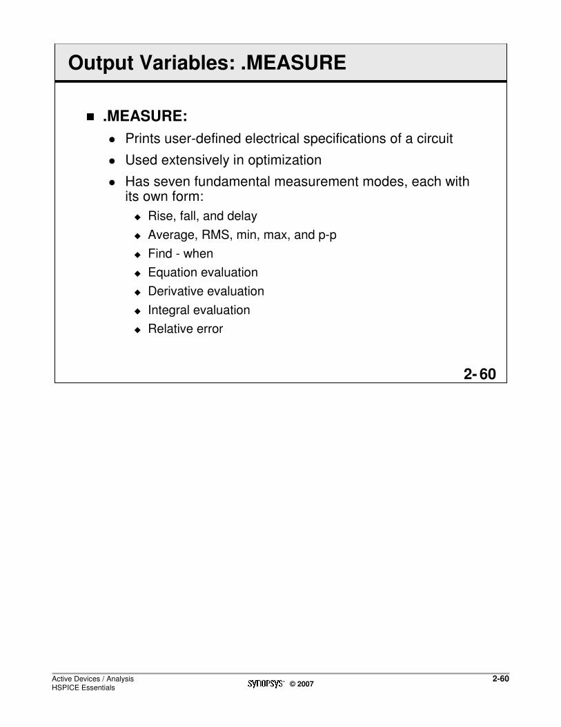
Active Devices / AnalysisHSPICE Essentials
2-60© 2007
602-
Output Variables: .MEASURE
� .MEASURE:
� Prints user-defined electrical specifications of a circuit
� Used extensively in optimization
� Has seven fundamental measurement modes, each with its own form:
� Rise, fall, and delay
� Average, RMS, min, max, and p-p
� Find - when
� Equation evaluation
� Derivative evaluation
� Integral evaluation
� Relative error

Active Devices / AnalysisHSPICE Essentials
2-61© 2007
612-
Output Variables: Parametric Output
� Parametric Output Variables:
.PRINT tran PAR(‘algebraic expression’)
.PRINT tran out_var=PAR(‘algebraic expression’)
Examples:
.PRINT dc conductance=PAR(‘i(m1)/v(22)’)
.PROBE tran PAR(‘log10(i(xff4.m1))’)
.PRINT tran vds=PAR(vds) vgs=PAR(vgs)

Active Devices / AnalysisHSPICE Essentials
2-62© 2007
622-
LAB 2: Devices and Subcircuits
During this lab, you will:
1. Use active devices
2. Construct a subcircuit
3. Use the subcircuit in a netlist
Active devices
Subcircuit
Netlist
45 minutes

Controls and OptionsHSPICE Essentials
3-1© 2007
13-
Agenda
© 2007 Synopsys, Inc. All Rights ReservedSynopsys 60-I-031-BSG-008
DAY
1111Introduction1
Active Devices / Analysis2
Controls and Options3
How Simulation Works4

Controls and OptionsHSPICE Essentials
3-2© 2007
23-
Unit Objectives
After completing this unit, you should be able to:
� Have a clear sense of how to set options
� Use simulation controls and options including:
� Input file control options
� Output control options
� OP and DC simulation controls
� Transient analysis accuracy and performance options
� Debugging options

Controls and OptionsHSPICE Essentials
3-3© 2007
33-
Overview of Options
� Syntax:
.OPTIONS opt1 <opt2 opt3> … <opt=x>
� Order independent
� Last definition is used
� ‘+’ in first column is continuation character
� .OPTIONS, .OPTION, .OPT are all the same
� .OPTION controls for:
� Input file control
� Search path for library, device scaling, model, etc
� Output and Interface
� Listing file control, output signal selection, output format control, etc
� Analyses control
� Algorithms
� Convergence aids
� Accuracy and performance control
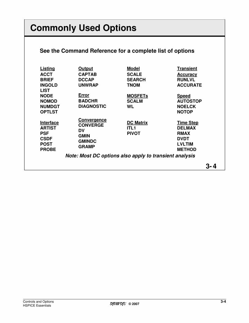
Controls and OptionsHSPICE Essentials
3-4© 2007
43-
Commonly Used Options
See the Command Reference for a complete list of options
Listing
ACCTBRIEF
INGOLDLIST
NODENOMOD
NUMDGTOPTLST
Interface
ARTIST
PSFCSDF
POSTPROBE
Output
CAPTABDCCAP
UNWRAP
Error
BADCHR
DIAGNOSTIC
Model
SCALESEARCH
TNOM
MOSFETsSCALM
WL
DC Matrix
ITL1
PIVOT
Transient
AccuracyRUNLVL
ACCURATE
SpeedAUTOSTOP
NOELCKNOTOP
Time Step
DELMAX
RMAXDVDT
LVLTIMMETHOD
ConvergenceCONVERGE
DVGMIN
GMINDC
GRAMP
Note: Most DC options also apply to transient analysis

Controls and OptionsHSPICE Essentials
3-5© 2007
53-
Understanding Options (1/2)
What options do YOU use?
Do you know what they do?
DCON?
ABSMOS?INTERP?
CSHUNT?
RELV?
SCALE?
CHGTOL?
?“Just set these...”
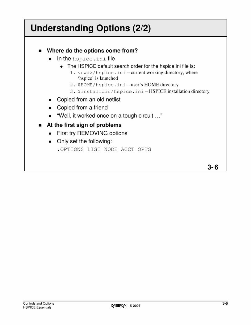
Controls and OptionsHSPICE Essentials
3-6© 2007
63-
Understanding Options (2/2)
� Where do the options come from?
� In the hspice.ini file
� The HSPICE default search order for the hspice.ini file is:
1. <cwd>/hspice.ini – current working directory, where
‘hspice’ is launched
2. $HOME/hspice.ini – user’s HOME directory
3. $installdir/hspice.ini – HSPICE installation directory
� Copied from an old netlist
� Copied from a friend
� “Well, it worked once on a tough circuit …”
� At the first sign of problems
� First try REMOVING options
� Only set the following:
.OPTIONS LIST NODE ACCT OPTS

Controls and OptionsHSPICE Essentials
3-7© 2007
73-
General Options: Listing File Options (1/5)
.option LIST
� Prints a list of netlist elements, node connections and, parameter values
� Prints effective sizes of elements and key values
� Useful in diagnosing topology-related problems
.option NODE
� Prints a node connection table
� The nodal cross-reference table lists each node and all the elements connected to it
� Useful in diagnosing topology related non-convergence problems

Controls and OptionsHSPICE Essentials
3-8© 2007
83-
General Options: Listing File Options (2/5)
.option ACCT
� Reports job accounting and runtime statistics at the end of the output listing
� Useful in observing simulation efficiency
.option OPTS
� Reports settings of all .OPTIONS in the listing file

Controls and OptionsHSPICE Essentials
3-9© 2007
93-
General Options: Listing File Options (3/5)
� Simulation listing files can get large
.option NOMOD
� Suppresses the printout of MODEL parameters
.option BRIEF=1
� Stops print back of data until an .OPTION BRIEF=0 or .END is encountered
� Resets the options LIST, NODE, and OPTS while setting NOMOD
� Re-enables print back after .OPTION BRIEF=0
� A good use of .OPTION BRIEF=1 is to place it in front of .MODEL statement definitions and .OPTION BRIEF=0after them

Controls and OptionsHSPICE Essentials
3-10© 2007
103-
General Options: Listing File Options (4/5)
.PROTECT / .UNPROTECT
� Suppresses the print back of the text from the list file
� Similar to .OPTION BRIEF
� Useful for making private models and cell libraries
� Place it directly in the .INCLUDE or .LIB files
� Restore normal print back with .UNPROT
� First sign of trouble:
� Remove all brief, nomod, and protect statements from all files so that you can see all information

Controls and OptionsHSPICE Essentials
3-11© 2007
113-
General Options: Listing File Options (5/5)
.option INGOLD=<value>
� Controls the format of numbers in printouts
� 0 – engineering format (default)
� 1 – mix of fixed and exponential format
� 2 – exponential format
.option NUMDGT =<value>
� Number of significant digits printed for output variables
� Range is between 1 to 10
� Defaults is 4

Controls and OptionsHSPICE Essentials
3-12© 2007
123-
General Options: Netlist Options SCALE (1/2)
� GLOBAL SCALE
� Scale element geometric instance parameters whose default unit is meters.
� SYNTAX
.option scale = <value>
Example:
.option scale = 1e-6
M1 Vdd 10 20 0 mymodel L=1u w=1u $ L=1e-12, W=1e-12
M2 Vdd 10 20 0 mymodel L=1 w=1 $ L=1e-6, W=1e-6
C1 Vdd 10 capmod L=0.1 W=0.1 $ L=1e-7, W=1e-7
R1 20 0 resmod L=1 W=1 $ L=1e-6, W=1e-6
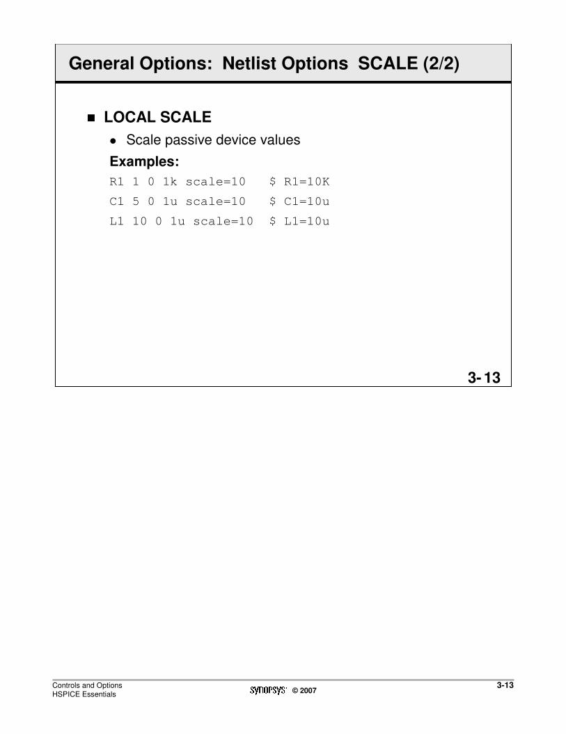
Controls and OptionsHSPICE Essentials
3-13© 2007
133-
General Options: Netlist Options SCALE (2/2)
� LOCAL SCALE
� Scale passive device values
Examples:
R1 1 0 1k scale=10 $ R1=10K
C1 5 0 1u scale=10 $ C1=10u
L1 10 0 1u scale=10 $ L1=10u
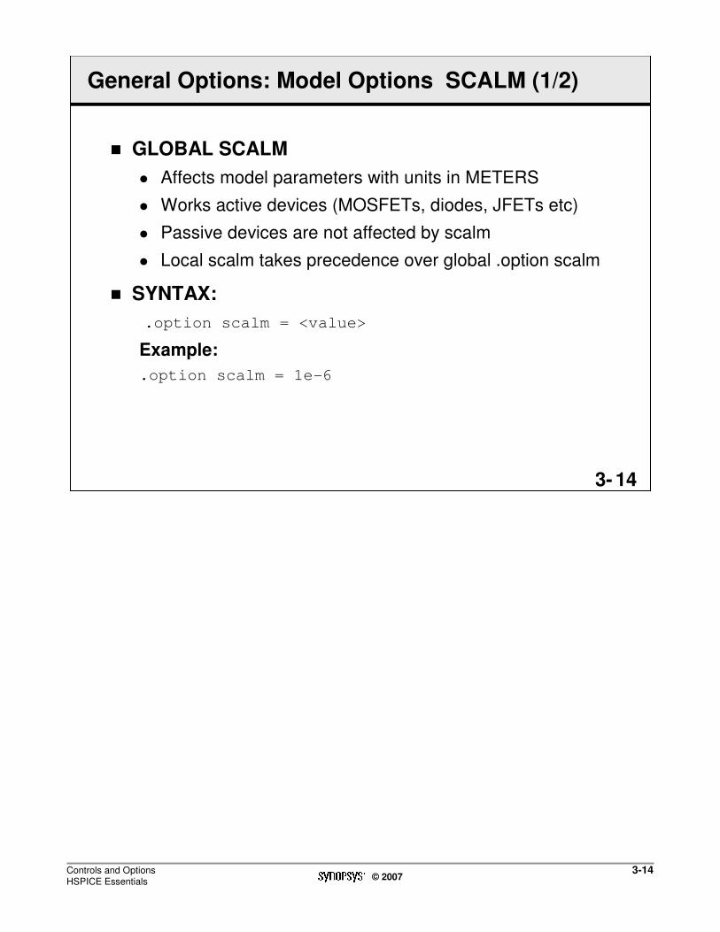
Controls and OptionsHSPICE Essentials
3-14© 2007
143-
General Options: Model Options SCALM (1/2)
� GLOBAL SCALM
� Affects model parameters with units in METERS
� Works active devices (MOSFETs, diodes, JFETs etc)
� Passive devices are not affected by scalm
� Local scalm takes precedence over global .option scalm
� SYNTAX:
.option scalm = <value>
Example:
.option scalm = 1e-6

Controls and OptionsHSPICE Essentials
3-15© 2007
153-
General Options: Model Options SCALM (2/2)
� LOCAL SCALM
� Affects model parameters with the units of meters
Example:
M1 Vdd 10 20 0 mymodel L=1u w=1u
.model mymodel nmos scalm=1e-6 level=2
+ tox=1e-1 kp=2.0e-5
� Only model parameters tox will be scaled
� tox=1e-7
� L and W will not be affected
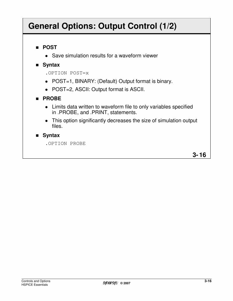
Controls and OptionsHSPICE Essentials
3-16© 2007
163-
General Options: Output Control (1/2)
� POST
� Save simulation results for a waveform viewer
� Syntax
.OPTION POST=x
� POST=1, BINARY: (Default) Output format is binary.
� POST=2, ASCII: Output format is ASCII.
� PROBE
� Limits data written to waveform file to only variables specifiedin .PROBE, and .PRINT, statements.
� This option significantly decreases the size of simulation output files.
� Syntax
.OPTION PROBE

Controls and OptionsHSPICE Essentials
3-17© 2007
173-
General Options: Output Control (2/2)
� POSTTOP
� Limits data written to waveform file to top-level nodes only
� Syntax
.OPTION POSTTOP
� POSTLVL
� Limits data written to waveform file that only a specified level of nodes signals will be saved
� Syntax
.OPTION POSTLVL=n
� n=1 top level
� n=0 all levels, i.e., POSTLVL option is turned off

Controls and OptionsHSPICE Essentials
3-18© 2007
183-
General Options: Performance Improvement (1/3)
� MODSRH
� Models not referenced in the circuit are not loaded
� Shortens simulation run time
� Syntax
.OPTION MODSRH=x
� Where
� x=1 - Enabled
� x=0 - Disabled
� Default has been enabled since the 2006.03 release
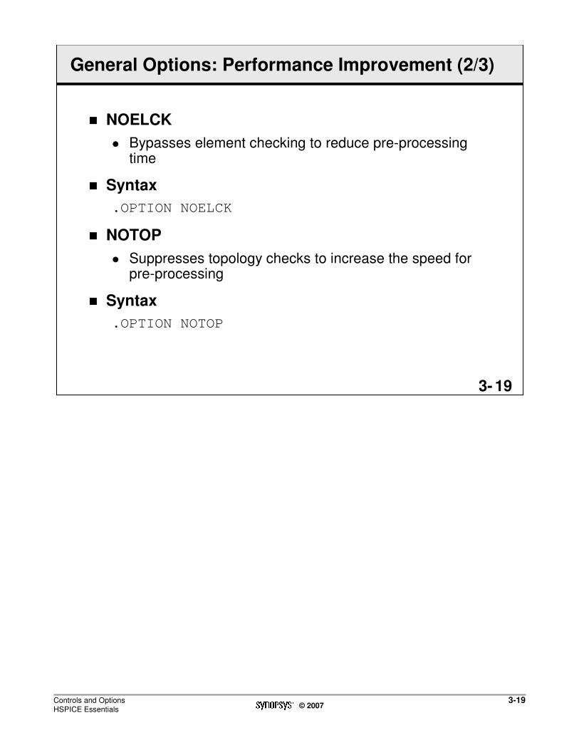
Controls and OptionsHSPICE Essentials
3-19© 2007
193-
General Options: Performance Improvement (2/3)
� NOELCK
� Bypasses element checking to reduce pre-processing time
� Syntax
.OPTION NOELCK
� NOTOP
� Suppresses topology checks to increase the speed for pre-processing
� Syntax
.OPTION NOTOP

Controls and OptionsHSPICE Essentials
3-20© 2007
203-
General Options: Performance Improvement (3/3)
� Linear matrix reduction
� Syntax
.option SIM_LA = PACE | PI
� Actives linear matrix reduction using PACT or PI algorithm
� Reduces matrices that represent RC networks to accelerate the simulation
� Preserve nodes used by any analysis statement, such as .PROBE, .MEASURE, etc
� .PROBE V(*) $ results in no reduction at all !
� Very effective for post-layout simulation
� Circuits with large volume of parasitic Rs and Cs

Controls and OptionsHSPICE Essentials
3-21© 2007
213-
OP and DC Simulation Controls (1/3)
� .option DCSTEP=<value>
� Default=0
Example:
.option dcstep=1e3
� Converts DC model and element capacitors to a conductance
� DC analysis opens all capacitors
� Divide capacitance by DCSTEP to model DC conductance
� Helpful in the case where there are “No DC Path to Ground” errors
� Helpful in the case where there is a “No Convergence in DC Solution” error

Controls and OptionsHSPICE Essentials
3-22© 2007
223-
OP and DC Simulation Control (2/3)
.option GMINDC=<value>
� Conductance in parallel to all pn junctions and MOSFET nodes except gate for DC analysis
� Default is 1e-12
.option SYMB=1
� Improve DC convergence for digital and mixed-signal circuit
Controls and OptionsHSPICE Essentials
3-23© 2007
233-
OP and DC Simulation Controls (3/3)
.option DCCAP
� Forces the voltage-variable capacitors to be evaluated during a DC sweep
� Generate C-V plots
� Used to review the basic transistor characteristics to diagnose a simulation or modeling problem
.option CAPTAB
� Prints a table of single-plate nodal capacitances for diodes, BJTs, MOS, JFETs, and passive capacitors at each operating point
� If there are a lot of nodes with small capacitances, chances are the parasitic capacitances are not in the models
� Look for nodes with less than 50ff of capacitance

Controls and OptionsHSPICE Essentials
3-24© 2007
243-
Transient Simulation Controls: RUNLVL (1/2)
� RUNLVL
� Syntax
.option RUNLVL=X
� Where X can be an integer between 0 and 6
� 0 -- turns option off
� 1 -- fastest
� 3 -- accuracy same as original HSPICE
� 5 -- accuracy same as original HSPICE with ACCURATE
� 6 -- most accurate
Controls and OptionsHSPICE Essentials
3-25© 2007
253-
Transient Simulation Controls: RUNLVL (2/2)
� Smarter timestep control speeds up transient simulation
� Especially digital circuits
� 3x average, up to 20x speedup on cell characterization
� Enhanced convergence
� less chance of encountering “time step too small” error
� Improved ease of use

Controls and OptionsHSPICE Essentials
3-26© 2007
263-
Transient Simulation Controls
� .option ACCURATE
� Tightens the simulation options to give the most accurate simulation algorithm and tolerances
� .option DELMAX=<value>
� Maximum allowed time step size
� .option BYPASS=1
� Do not evaluate latent devices
� Applies to MOSFETs, MESFETs, JFETs, BJTs, and diodes
� Default is 1
� .option AUTOSTOP
� Stops a transient analysis in HSPICE after calculating all TRIG-TARG, FIND-WHEN, and FROM-TO measure functions
� Special interest when testing corners

Controls and OptionsHSPICE Essentials
3-27© 2007
273-
LAB 3: Simulation Controls and Options
Experience the effect of using simulation control options
Simulation
Controls
Options
45 minutes

Controls and OptionsHSPICE Essentials
3-28© 2007
This page was intentionally left blank.

How Simulation WorksHSPICE Essentials
4-1© 2007
14-
Agenda
© 2007 Synopsys, Inc. All Rights ReservedSynopsys 60-I-031-BSG-008
DAY
1111Introduction1
Active Devices / Analysis2
Controls and Options3
How Simulation Works4

How Simulation WorksHSPICE Essentials
4-2© 2007
24-
Unit Objectives
After completing this unit, you should be able to:
� Explain how simulation works
� Explain convergence and non-convergence
� Explain how the DC operating point is calculated

How Simulation WorksHSPICE Essentials
4-3© 2007
34-
Simulation Controls and Convergence
� How Simulation Works:
� Linearization
� Newton-Raphson
� Non-convergence:
� General Aids
� Non-convergence aids for DC Operating Point Analysis

How Simulation WorksHSPICE Essentials
4-4© 2007
44-
How Simulation Works (1/2)
� Spice begins by writing a set of nodal equations to describe the elements in the circuit:
� Engineers begin by writing only 2 or 3 equations
� Reduce to a simple algebraic form and solve
G * V = I
Vr
Ir
Resistor
Slope = 1/R = Gr

How Simulation WorksHSPICE Essentials
4-5© 2007
54-
How Simulation Works (2/2)
� Computers solve via matrix methods:
� Solve simultaneous equations using Gaussian Elimination
G11 G12 G13 ...
G21 G22 ...G31 ...
.
.
.
V1
V2V3
.
.
.
I1I2
I3
.
.
.
*=
+
-
V
V1 V2 V3

How Simulation WorksHSPICE Essentials
4-6© 2007
64-
The Matrix (1/2)
� Linear representation between voltage and current for every element in the circuit
� Voltage array:
� The solution array
� HSPICE tries to determine the node voltage values, which satisfy Kirchhoff’s voltage and current laws for the circuit
� Current array:
� Known value of the circuit
� Represents the independent branch currents generated from current sources and active devices
� HSPICE determines the branch currents from the current source settings, or from the previous voltages applied to the active device terminals

How Simulation WorksHSPICE Essentials
4-7© 2007
74-
The Matrix (2/2)
� Conductance Array:
� Known value of the circuit
� Represents the linear relationship between voltage and current for every element in the circuit
� Nonlinear elements are represented in the conductance array by their linear equivalent circuits
� Entries in the Current and Conductance arrays are used to determine the next set of solution voltages

How Simulation WorksHSPICE Essentials
4-8© 2007
84-
Introduction of Nonlinear Elements (1/3)
� Simple … UNTIL … nonlinear elements are introduced:
� Problem because the matrices represent LINEAR relationships
� Diodes, capacitors, transistors, etc. have current-voltage relationships that change in response to the DC bias of the circuit
� Solutions no longer take on algebraic form
� 7x + x = 32
� Solutions are now transcendental in form
� 7x + exp(x) = 32

How Simulation WorksHSPICE Essentials
4-9© 2007
94-
Introduction of Nonlinear Elements (2/3)
� Solution:
� Break the nonlinear I-V relationships into many smaller linear approximations
� The linear equivalent is determined by the bias voltage
� At each step in the analysis, HSPICE uses the linear equivalent circuit to represent the device at its bias voltage
� Known as Linearization

How Simulation WorksHSPICE Essentials
4-10© 2007
104-
Introduction of Nonlinear Elements (3/3)
� Diode Example
� If the solution voltage is close to the voltage Vb, the only part of the I-V characteristic of interest to the simulator are the I-V characteristics close to Vb
� The nonlinear characteristics may be represented by a straight-line approximation equal to the tangent of the diode characteristics
� The result is a straight-line model of the diode
� Newton-Raphson algorithm used to solve matrix
Vd
Id
Diode
Vd
Id
VbIeq
Id = Vd*Gd + Ieq
Diode

How Simulation WorksHSPICE Essentials
4-11© 2007
114-
Linear vs. Small Signal Model
� Similar, but not the same
� Linear Model:
� Dynamic conductance, Gd and, the equivalent current, Ieq and, may contain small-signal capacitance if transient analysis is being performed
� Small-Signal Model:
� Dynamic resistance 1/gd and, small-signal capacitance, Cd
Vd =
Id +
-
+
-
Ieq
+
-
Vd
Id
Gd
Linear
Id
gdcd
+
-
Vd
Small Signal
How Simulation WorksHSPICE Essentials
4-12© 2007
124-
Linearization (1/2)
� Linearization of Transistors:
� Extending the diode model …
� Process must account for every pair of device terminals
� Charge-storage Elements:
� More complex … IV characteristics of C and L change with applied voltage, current, and time
� During transient analysis, numerical integration routines are involved
� Solution points are now discrete moments in time

How Simulation WorksHSPICE Essentials
4-13© 2007
134-
Linearization (2/2)
� The point here is to illustrate the increasing complexity of the process: adding diodes and adding companion models (for charge)
� Mosfet Transistors:
� Gate-source, drain-source, source-drain, source-bulk terminals must all be linearized before storing in the system equations
� Bipolar Transistors:
� Base-emitter, collector-emitter, collector-base terminals must be linearized

How Simulation WorksHSPICE Essentials
4-14© 2007
144-
Newton-Raphson: Solving the Matrix (1/2)
� Once the conductance and current arrays are filled, HSPICE must solve the node-voltage equations in the voltage arrays:
� Two methods
� For linear elements: Gaussian Elimination
– 7x + x = 32
� For nonlinear elements: Newton-Raphson formula
– ln(x) + x = 32

How Simulation WorksHSPICE Essentials
4-15© 2007
154-
Newton-Raphson: Solving the Matrix (2/2)
� Iterative Guessing Technique:
� Begins the process with an initial guess
� Finds the solution through a series of successive guesses
� HSPICE uses f(x) to guess the next value
� Not random
x f(x)
f(x) = ln(x) + x -32
1
10
20
.
.
28.65
28.645
-31
-19.7
-9
.
.
.005
.000021
“random
guessing”

How Simulation WorksHSPICE Essentials
4-16© 2007
164-
Newton-Raphson Method
� Newton-Raphson Formula:
Xn+1 = Xn - [F(Xn) / F’(Xn)]
� F’(x) represents the derivative
� Note that since this is the denominator, a slope of zero (zero conductance) is disastrous
� GMIN is used to keep this slope from ever being zero
� HSPICE uses the Newton-Raphson algorithm when 1 or more nonlinear devices are entered in the circuit
� HSPICE starts with an initial guess for every node voltage in the circuit and begins iterating
� With each successive iteration, a new set of node voltages is predicted

How Simulation WorksHSPICE Essentials
4-17© 2007
174-
Newton-Raphson: Solving the Matrix (1/2)
� Terminating the Iterative Process:
� Newton-Raphson algorithm monitors the node voltage of the present iteration and the previous iteration value
� Successful Termination:
� HSPICE monitors the difference between these iterative values and compares the difference with a predefined error tolerance
� Delta between iterative voltage values less than a predefined error tolerance

How Simulation WorksHSPICE Essentials
4-18© 2007
184-
Newton-Raphson: Solving the Matrix (2/2)
� Unsuccessful Termination:
� HSPICE limits the total number of iterations each analysis type is allowed to process
� HSPICE exceeds the iteration limit
� Non-convergence
� Timestep is smaller than allowed minimum timestep
� “Timestep too small” error

How Simulation WorksHSPICE Essentials
4-19© 2007
194-
Newton-Raphson: Termination Criteria (1/2)
/* NC is the # of non-convergent nodes, currents, or MOSFETs
Another Iteration: Iteration_Number = Iteration_Number + 1
NC=0
Do I=1, # Circuit Nodes
if ( | V(n) - V(n-1) | > RELV * V(n) + ABSV) then NC = NC + 1
Do I =1, # Branch Currents
if ( | I(n) - I(n-1) | > RELI * I(n) + ABSI) then NC = NC + 1
Do I=1, # MOSFETs
if ( | Ids(n) - Ids(n-1) | > RELMOS * Ids(n) + ABSMOS then NC = NC + 1
IF NC = 0
Save Solution
else
If (Iteration_Number < Iteration_Limit) do Another_Iteration
else Failed_to_Converge

How Simulation WorksHSPICE Essentials
4-20© 2007
204-
Newton-Raphson: Termination Criteria (2/2)
Number of Iterations
Error
BetweenIterations
Iteration_Limit (ITL1)
| Vn - Vn-1 |or
| In - In-1 |
RELV * Vn + ABSV
0
Error Tolerance

How Simulation WorksHSPICE Essentials
4-21© 2007
214-
What is Non-convergence?
� Definition:
� Failure to find a set of node voltages and branch currents that conform to Kirchhoff’s voltage and current laws within specified iteration loop limitations
� Dreaded words:
� “No Convergence in DC Solution”
� “Timestep too Small”

How Simulation WorksHSPICE Essentials
4-22© 2007
224-
Non-convergence
Possible Causes:
Node Unstable
Circuit
Reason
Model
Problem
Simulator
Options
Feedback
Parasitics
Negative Conductance
Model Discontinuity
Tolerances
Algorithms
Incomplete Netlist
Algorithms

How Simulation WorksHSPICE Essentials
4-23© 2007
234-
Non-convergence - General Aids (1/2)
� Check Topology:
� Remove all options except post, list, acct, node and opts
� Units (Scale, Scalm, large values)
� Review element sizes in listing file
� Review listing file for .param substitution listing
� Search the listing file for “warning” and “error”
� Break the circuit into smaller pieces
� Simplify input sources

How Simulation WorksHSPICE Essentials
4-24© 2007
244-
Non-convergence - General Aids (2/2)
� Circuit conductance values:
� Determine parallel resistance that can be placed across any 2 nodes without influencing circuit behavior
� Models:
� Check active device models for resistance and capacitance parameters
� Error Tolerances:
� Set RELV, RELI, RELMOS
� Then set ABSV, ABSI, ABSMOS
How Simulation WorksHSPICE Essentials
4-25© 2007
254-
Convergence: Tolerances (1/3)
� Error tolerances determine accuracy and speed of the simulation:
� Default settings usually produce acceptable accuracy with reasonable runtime
� Some circuits require more accuracy. Some less
� Proper Selection of HSPICE error tolerances:
� “What % of error can you accept”
� Requires knowledge of the voltage and current levels of the circuit
� Determine Vsmall: smallest voltage of interest in the circuit
� Determine Ismall: the smallest current magnitude of interest in the circuit
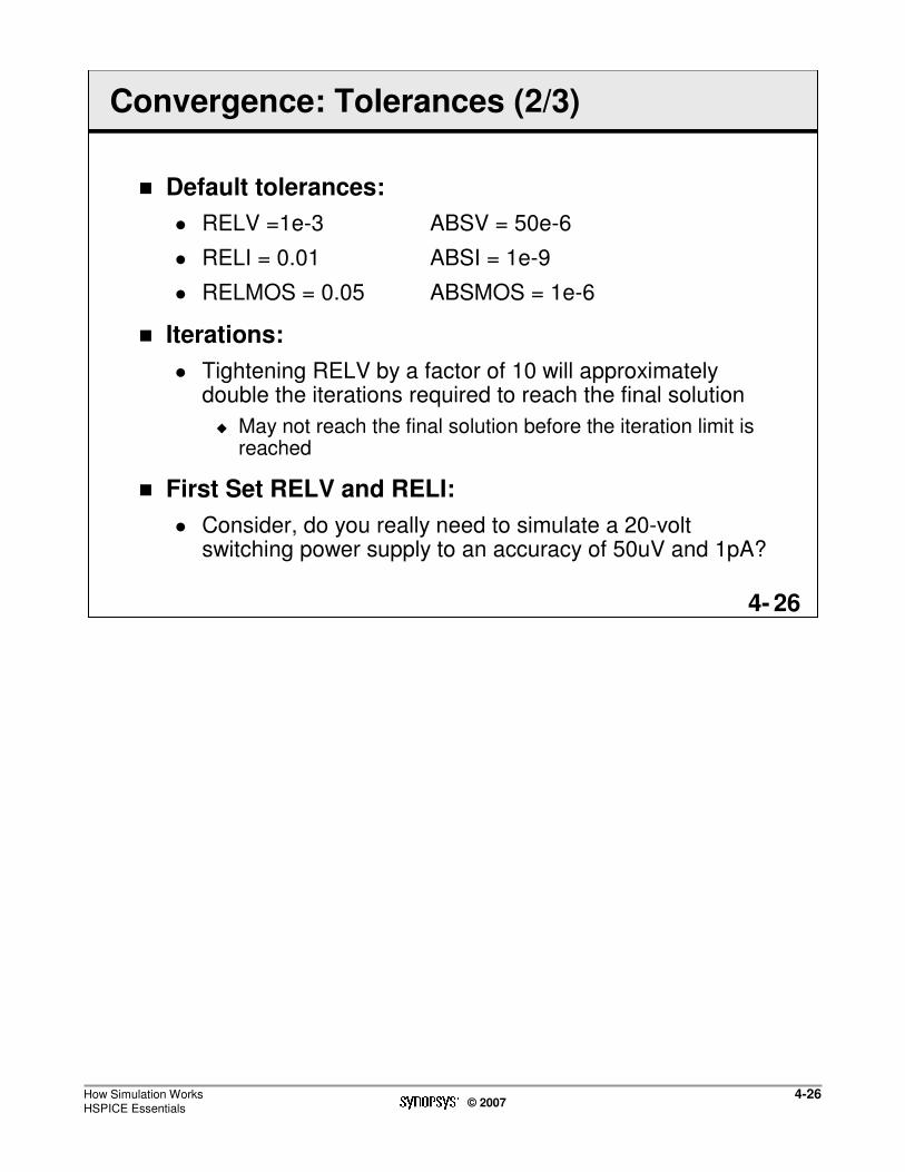
How Simulation WorksHSPICE Essentials
4-26© 2007
264-
Convergence: Tolerances (2/3)
� Default tolerances:
� RELV =1e-3 ABSV = 50e-6
� RELI = 0.01 ABSI = 1e-9
� RELMOS = 0.05 ABSMOS = 1e-6
� Iterations:
� Tightening RELV by a factor of 10 will approximately double the iterations required to reach the final solution
� May not reach the final solution before the iteration limit is reached
� First Set RELV and RELI:
� Consider, do you really need to simulate a 20-volt switching power supply to an accuracy of 50uV and 1pA?
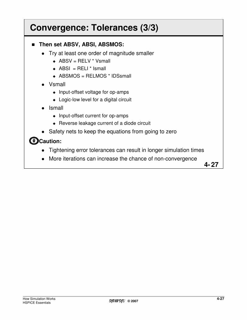
How Simulation WorksHSPICE Essentials
4-27© 2007
274-
Convergence: Tolerances (3/3)
� Then set ABSV, ABSI, ABSMOS:
� Try at least one order of magnitude smaller
� ABSV = RELV * Vsmall
� ABSI = RELI * Ismall
� ABSMOS = RELMOS * IDSsmall
� Vsmall
� Input-offset voltage for op-amps
� Logic-low level for a digital circuit
� Ismall
� Input-offset current for op-amps
� Reverse leakage current of a diode circuit
� Safety nets to keep the equations from going to zero
Caution:
� Tightening error tolerances can result in longer simulation times
� More iterations can increase the chance of non-convergence

How Simulation WorksHSPICE Essentials
4-28© 2007
284-
Convergence: Conductance Values (1/2)
� Conductance term used to predict the next voltage value
� Problem: If conductance becomes small, 2nd term becomes large:
� Next voltage value unrealistic
� Causes extra iterations
� Worse: Conductance of zero!
Vn+1 = Vn -G(Vn)
F(Vn)
I
V
G(Vn)=0

How Simulation WorksHSPICE Essentials
4-29© 2007
294-
Convergence: Conductance Values (2/2)
� Since all semiconductor device models contain regions of zero conductance:
� Shunt R placed in parallel with every PN junction and drain to source
� Determine smallest parasitic Rp that can be placed across any 2 nodes without influencing circuit behavior
� G=1/Rp
� Try setting .OPTION GMINDC=1e-9 GMIN=1e-9
� Default for both GMIN and GMINDC is 1e-12

How Simulation WorksHSPICE Essentials
4-30© 2007
304-
Convergence: Diode Resistance (1/2)
� High conductance is troublesome to the algorithm:
� Highly forward-biased diodes (greater than 0.8V)
� Leads to very small iteration-to-iteration voltage changes
� HSPICE can reach ITL1 limit before reaching the proper solution voltage
I
VnVn+1
Final Solution Voltage
Small iteration voltage changes
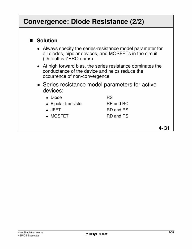
How Simulation WorksHSPICE Essentials
4-31© 2007
314-
Convergence: Diode Resistance (2/2)
� Solution
� Always specify the series-resistance model parameter for all diodes, bipolar devices, and MOSFETs in the circuit (Default is ZERO ohms)
� At high forward bias, the series resistance dominates the conductance of the device and helps reduce the occurrence of non-convergence
� Series resistance model parameters for active devices:
� Diode RS
� Bipolar transistor RE and RC
� JFET RD and RS
� MOSFET RD and RS

How Simulation WorksHSPICE Essentials
4-32© 2007
324-
Non-convergence-General Aids: Summary
� Topology Check
� Break the circuit up
� Simplify input sources
� Circuit Conductance Values
� GMIN and GMINDC options
� Diode Resistance
� Error Tolerance

How Simulation WorksHSPICE Essentials
4-33© 2007
334-
Four Basic Simulation Types
� DC Operating/Bias Point Analysis
� DC Sweep Analysis
� AC Frequency Analysis
� Transient Analysis
� Only three analyses fail from non-convergence:
� DC operating point
� DC sweep
� Transient analysis
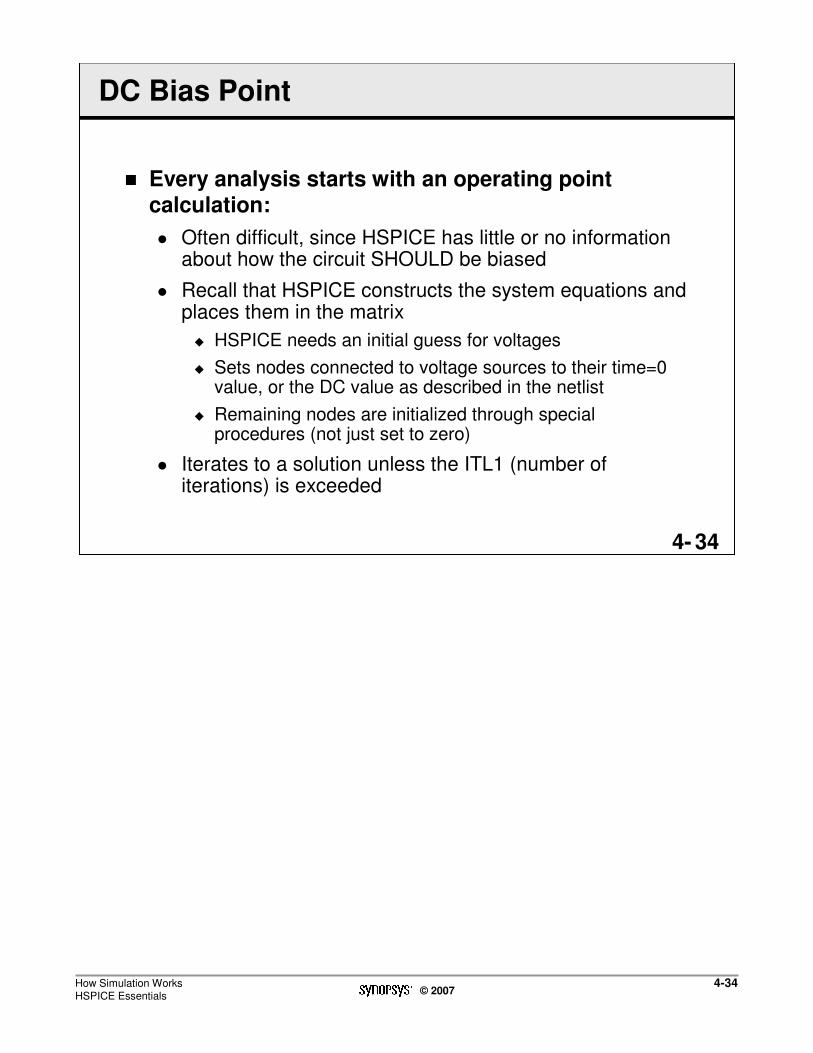
How Simulation WorksHSPICE Essentials
4-34© 2007
344-
DC Bias Point
� Every analysis starts with an operating point calculation:
� Often difficult, since HSPICE has little or no information about how the circuit SHOULD be biased
� Recall that HSPICE constructs the system equations and places them in the matrix
� HSPICE needs an initial guess for voltages
� Sets nodes connected to voltage sources to their time=0 value, or the DC value as described in the netlist
� Remaining nodes are initialized through special procedures (not just set to zero)
� Iterates to a solution unless the ITL1 (number of iterations) is exceeded
How Simulation WorksHSPICE Essentials
4-35© 2007
354-
DC Non-Convergence
� HSPICE DC bias non-convergence aids:
� Auto-converge process
� .NODESET/.IC
� Symbolic operating point
� Model-related
� Other, less impact
� DCSTEP and GMINDC ramping
� Source stepping/ramping
� GSHUNT/CSHDC
� DV

How Simulation WorksHSPICE Essentials
4-36© 2007
364-
DC Bias Point Convergence Aids
� Remove all options except ACCT, NODE, LIST, POST and OPTS
� Allow the auto converge process to proceed
� Review the .lis file for convergence hints
� Search for “warning” and “error”
� Rerun the simulation

How Simulation WorksHSPICE Essentials
4-37© 2007
374-
DC Auto-convergence Process (1/5)
� Step 1 - Newton Raphson Method (SPICE standard):
� Iterate up to the ITL1 limit
� Converged? Yes – results, No - Step 2
� Step 2:
� Set DCON=1
� Tighten DV from 1000 to 0.1
� DV - maximum iteration-to-iteration voltage change for all circuit nodes in both DC and transient analysis
� Use GMINDC Ramping method
� Set GRAMP=6
� Ramp GMINDC 1e-6 to 1e-12
� Increase ITL1 = ITL1 + 20 * GRAMP
� Converged? Yes – results, No – Step 3

How Simulation WorksHSPICE Essentials
4-38© 2007
384-
DC Auto-convergence Process (2/5)
� Step 3:
� Set DCON=2
� Use GMINDC Ramping method
� Loosen DV to 1,000,000
� Set GRAMP=6
� Ramp GMINDC 1e-6 to 1e-12
� Increase ITL1 = ITL1 + 20 * GRAMP
� Converged? Yes – results, No – Step 4

How Simulation WorksHSPICE Essentials
4-39© 2007
394-
DC Auto-convergence Process (3/5)
� Step 4:
� Use Damped Pseudo Transient Method
� Add CSHDC and GSHUNT from each node to ground
� Ramp supplies from 0 to set values
� After DC convergence remove CSHDC and GSHUNT
� Iterate to find stable bias point
� Converged? Yes – results, No- Step 5

How Simulation WorksHSPICE Essentials
4-40© 2007
404-
DC Auto-convergence Process (4/5)
� Step 5:
� Use GMATH Ramping Method
� Converged? Yes – results, No – non-convergence report
� GMATH is similar to the Pseudo-Transient method, except it does not ramp sources
� All sources keep their assigned DC values
� Add CSHDC from each node to ground
� Ramp gmath=cshdc/delta in the range 1e-12 to 10.0
� Delta is the pseudo-transient timestep
� Set gmath=0, if convergence occurs with gmath>1e-12, iterate to find stable bias point, same as step 1
� Converged? Yes – results, No – Step 6

How Simulation WorksHSPICE Essentials
4-41© 2007
414-
DC Auto-convergence Process (5/5)
� Step 6:
� Use GSHUNT ramping method
� Ramping the GSHUNT parameter from 1e-4 to 0
� Obtains solutions at every GSHUNT point by invoking Newton-Raphson, GMIN ramping, and pseudo-transient algorithms
� Converged? Yes – results, No – non-convergence report

How Simulation WorksHSPICE Essentials
4-42© 2007
424-
DC Bias Point: .NODESET and .IC (1/2)
� Non-convergence can happen due to poor initial conditions:
� Set initial conditions and/or nodesets
� .IC v(1)=5v v(abc)=0v v(12)=VDD
� .NODESET v(x1.87)=5v
Which nodes?
� Observe the non-convergent diagnostic table in the listing file
� Identify non-convergent nodes with unusually high voltages, branch currents, or high error tolerances
� Initialize these nodes
� Look at the circuit for un-initialized feedback paths (flip-flops, oscillators, etc)

How Simulation WorksHSPICE Essentials
4-43© 2007
434-
DC Bias Point: .NODESET and .IC (2/2)
� Inefficient to manually add .NODESET and/or .IC for a large number of nodes
� To set a large number of nodes
� Comment out all analysis commands except .TRAN
� Add UIC to the end of the .TRAN command
� Disable auto-convergence process
� .option DCON=-1 CONVERGE=-1
� Use .save <TYPE=nodeset | ic> <TIME=x> to store the calculated operating point in an .ic or .nodeset file and use .load for loading the file
� Simulate the circuit
� Use .load for loading the file from SAVE command, re-set all appropriate options, e.g. DCON / CONVERGE, remove UIC from .TRAN command.
� Re-simulate the circuit

How Simulation WorksHSPICE Essentials
4-44© 2007
444-
DC Bias Point: Symbolic Operating Point
� Improves circuitry convergence, especially digital circuits
� Assumes the circuit is digital and assigns a low or high state to all nodes
� Sets a reasonable initial guess to every voltage node
� Best for designs made with chains of standard cells
� Will not affect any other convergence options
� Syntax
.option SYMB=1

How Simulation WorksHSPICE Essentials
4-45© 2007
454-
DC Bias Point: Model Related (1/2)
� Inappropriate model parameters are most likely the cause:
� Units
� Zero or negative conductance
� Units:
� .OPTION SCALM (global)
� .MODEL SCALM factor (local value within .MODEL statements)
Is a global .OPTION SCALM needed?
� Look at listing file and review element values
� Swap in a KNOWN GOOD MODEL

How Simulation WorksHSPICE Essentials
4-46© 2007
464-
DC Bias Point: Model Related (2/2)
� Zero or Negative Conductance:
� HSPICE automatically prints out the first occurrence of “negative conductance” in the listing file
� gm, gds, gmbs, ids are all printed with the operating point
� Causes:
� Often caused by modeling problems in the subthreshold equations (if in cutoff) or channel length modulation equations (if in saturation)
� The magnitude reported indicates the magnitude of conductance (leakage) that must be placed across the drain and source to offset the effect (.option GMINDC and GMIN)
V
I
Region of Negative Conductance(Negative slope)

How Simulation WorksHSPICE Essentials
4-47© 2007
474-
Analysis Options: DIAGNOSTIC
� HSPICE automatically prints out the first occurrence of “negative-mos conductance” in the .lis file
� .option DIAGNOSTIC
� Causes all occurrences of negative model conductances to be printed in the .lis file
� If the magnitude of the negative conductance is > -1e-8, consult your modeling department or foundry

How Simulation WorksHSPICE Essentials
4-48© 2007
484-
DC Bias Point: Summary
� Auto-Converge Process:
� Remove .options and allow auto-converge procedure to work
� Increase ITL1 value (default=200)
� .NODESET/.IC
� Symbolic operating point
� .option SYMB
� Model-related:
� Review units
� Try known good model
� Other, Less Impact:
� DCSTEP and GMINDC Ramping
� .option converge=2
� Source Stepping/Ramping
� .option converge=3
� Set .option GSHUNT=<val> and/or CSHDC=<val>
� Set .option DV=<val>

How Simulation WorksHSPICE Essentials
4-49© 2007
494-
LAB 4: DC Bias Point
During this lab, you will examine how HSPICE converges to a DC bias point.
HSPICE
DC convergence
Nodesets
Initial conditions
45 minutes

How Simulation WorksHSPICE Essentials
4-50© 2007
This page was intentionally left blank.

ConvergenceHSPICE Essentials
5-1© 2007
15-
Agenda
© 2007 Synopsys, Inc. All Rights Reserved
DAY
2222Convergence5
Advanced Input Elements6
Customer SupportCS
Synopsys 60-I-031-BSG-008
ConvergenceHSPICE Essentials
5-2© 2007
25-
Unit Objectives
After completing this unit, you should be able to:
� Perform DC sweep
� Explain transient analysis
� Explain the causes of non-convergence and the possible solutions
� Explain numeric integration

ConvergenceHSPICE Essentials
5-3© 2007
35-
DC Sweep and Convergence Aids
� Similar to performing DC bias calculation:
� To begin a sweep, HSPICE performs a DC bias point calculation
� Once found, node voltages are saved and used as the initial guess for the next point in the sweep analysis
� Problems are somewhat different though
� Non-convergence mechanisms associated with DC sweep:
� Rapid voltage or current transitions
� Model discontinuities

ConvergenceHSPICE Essentials
5-4© 2007
45-
DC Sweep: Rapid Transitions
� Progression of analysis:
� Bias point found
� Input voltage raised to the first step in the sweep
� Bias point voltages used as the initial guess for the next set of ITL2 iterations
� ITL2 is the number of iterations allowed at each step in the DC sweep analysis
� Default is 50 Voltage transition is too large for the
Newton iterations to find a solution
Vin
Vout
Bias
Point No Solution Found
Individual Sweep Points

ConvergenceHSPICE Essentials
5-5© 2007
55-
DC Iteration Controls
� Action:
� Increase ITL2 to 100, 200 or more
� If you increase ITL2 to 400 and HSPICE still does not converge, it is unlikely that increasing ITL2 any further will improve the situation
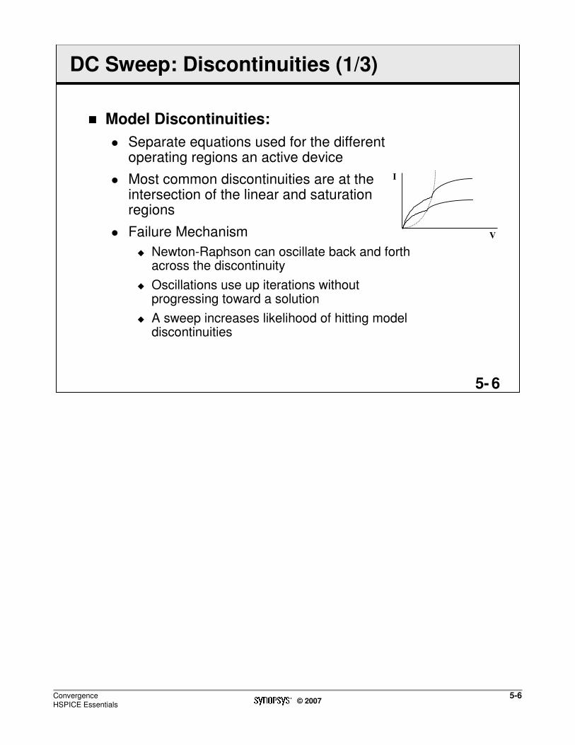
ConvergenceHSPICE Essentials
5-6© 2007
65-
DC Sweep: Discontinuities (1/3)
� Model Discontinuities:
� Separate equations used for the different operating regions an active device
� Most common discontinuities are at the intersection of the linear and saturation regions
� Failure Mechanism
� Newton-Raphson can oscillate back and forth across the discontinuity
� Oscillations use up iterations without progressing toward a solution
� A sweep increases likelihood of hitting model discontinuities
I
V

ConvergenceHSPICE Essentials
5-7© 2007
75-
DC Sweep: Discontinuities (2/3)
� Model discontinuity failure:
� Consider Conductance vs Voltage
� Conductance (G) predicts the next voltage iteration
� Model discontinuities only pose a problem if the solution steps align with, or fall very close to, the discontinuity
Gd = dId / dVd
Gd
VV0 V1
V1
Gd
VV0 V1
V2

ConvergenceHSPICE Essentials
5-8© 2007
85-
DC Sweep: Discontinuities (3/3)
� Actions:
� Increase or offset the analysis step size
� Obtain better models
Example of increasing or offsetting step size:
� Original analysis specification that does not converge
� .DC VIN 0v 5v .1v
� Increase step size
� .DC VIN 0v 5v .2v
� Offset step size
� .DC VIN .01v 5.01v .1v

ConvergenceHSPICE Essentials
5-9© 2007
95-
DC Sweep Analysis: Summary
� Non-convergence mechanisms associated with DC sweep:
� Rapid voltage or current transitions
� Action
� Increase ITL2 to 100, 200 or more
.OPTION ITL2=100
� Model discontinuities
� Increase or offset the analysis step size
� obtain better models

ConvergenceHSPICE Essentials
5-10© 2007
105-
AC Sweep and Convergence Aids
� AC frequency sweep analysis WILL ALWAYS CONVERGE:
� AC frequency sweep is a linear small-signal analysis that does not include any nonlinear behavior after the bias point is found
� Progression of Analysis:
� Calculate DC bias point
� Replace nonlinear device models with linear small-signal equivalents
� Use Gaussian elimination
� No Newton iterations are required
� Failure Mechanism:
� Calculation of DC bias point
� Action:
� Review DC bias point and convergence aids

ConvergenceHSPICE Essentials
5-11© 2007
115-
Transient and Convergence Aids
� General
� Dynamic Timestep Control
� Non-convergence:
� Rapid voltage transitions
� Model discontinuities
� Corrective Actions:
� High probability
� Device model capacitance
� GEAR integration
� Reduce TSTEP
� Use RUNLVL option
� Low probability
� Increase iteration limit

ConvergenceHSPICE Essentials
5-12© 2007
125-
Transient Analysis: General
� Progression of Analysis:
� DC bias point calculated first
� C - open, L - short
� Restore caps and inductors
� Element line IC can specify T0 initial conditionsCB B 0 10P IC=4V
LLD1 10 15 1.5U IC=5MA
� Transient sources established at T0 values
� Newton iterations begin at the first time point of the analysis
� At each new time point
� Newton iterations begin again
� As Newton iterates, numeric integration algorithms determine the capacitor currents and inductor voltages as a function of time

ConvergenceHSPICE Essentials
5-13© 2007
135-
Transient Analysis: Timestep Control
� Dynamic Timestep
� No longer a preset step size
� Step size changes on-the-fly
� Not the .TRAN tstep value, but is related
� TSTEP is the print interval for .PRINT command
� Maximum internal timestep is
min[(TSTOP/50), DELMAX, (TSTEP*RMAX)]
Default RMAN=5, DELMAX=100n
� Minimum internal timestep is
TSTEP*RMIN
Default RMIN=1n

ConvergenceHSPICE Essentials
5-14© 2007
145-
Dynamic Timestep Control Algorithms (1/3)
� LVLTIM Option
� Selects timestep algorithm used for transient analysis
� Syntax
.option LVLTIM=n
� LVLTIM=1 (default)
� For LVLTIM=1 or LVLTIM=3
� DVDT algorithm
� Unique to HSPICE
� Applies to digital CMOS design
� Based on the rate of change of nodal voltages
� For LVLTIM=3
� Use DVDT timestep control method with timestep reversal

ConvergenceHSPICE Essentials
5-15© 2007
155-
Dynamic Timestep Control Algorithms (2/3)
� For LVLTIM=2
� Local Truncation Error (LTE, SPICE standard):
� Timestep is reduced if actual error is > predicted error
� For LVLTIM=0
� Iteration Count (SPICE standard):
� If iterations required to converge > IMAX, decrease the timestep
– Default IMAX = 8
� If iterations required to converge < IMIN, increase the timestep
– Default IMIN =3
� For all transient timestep control algorithms, the iteration count method applies:
� For each new time point, if # iterations > IMAX, then go back tothe previous time point and cut the timestep

ConvergenceHSPICE Essentials
5-16© 2007
165-
Dynamic Timestep Control Algorithms (3/3)
� For DVDT and LTE:
� If # iterations < IMAX, then other criteria is also apply as to timestep control:
� For DVDT:
� The max voltage change allowed from time point to time point is set by the options RELVAR and ABSVAR
� .option REVLAR ( default = 0.3, i.e. 30%)
� .option ABSVAR ( default =0.5 v )
� Timestep reversal, (LVLTIM = 3)
– If the different between the current solution and the previous one is greater than the max voltage, HSPICE discards the solution, sets the timestep to a smaller value and recalculates the
solution.
� For LTE, accepting the current solution also depends on CHGTOL, RELTOL, and RELQ

ConvergenceHSPICE Essentials
5-17© 2007
175-
Transient: Non-convergence (1/2)
� Timestep too small occurs when:
� Internal timestep < RMIN * TSTEP
� TSTEP from .TRAN statement
� .option RMIN=x
– Default=1n

ConvergenceHSPICE Essentials
5-18© 2007
185-
Transient: Non-convergence (2/2)
� Convergence Failures:
� Rapid voltage transitions
� Model discontinuities
� Rapid Voltage Transitions:
� Dynamic timestep control automatically reduces the timestep size
� As circuit approaches a voltage transition, two potentially conflicting events occur
� Semiconductor devices are switching from one region of operation to another
� Timestep is reduced
� Model Discontinuities:
� Discussion in DC sweep applies

ConvergenceHSPICE Essentials
5-19© 2007
195-
Transient Analysis: Corrective Actions (1/4)
� High Probability Correction Actions:
� Device Model Capacitance
� All device models have a built-in capacitance (junction or overlap)
� These capacitive currents help bridge the discontinuity
� Unfortunately, these capacitances default to ZERO
� All simulation models should have their associated capacitance terms set to a nonzero value
– Real models have real capacitances
� Capacitive Model Parameters:
� Diode CJO
� Bipolar CJE, CJC, CJS
� JFET CGD, CGS
� MOSFET CGDO, CGSO, CGDO, CBD, CBS, CJ, CJSW

ConvergenceHSPICE Essentials
5-20© 2007
205-
Transient Analysis: Corrective Actions (2/4)
� GEAR Integration:
� Numeric integration of time varying currents and voltages are accomplished through Trapezoidal and Gear linearization
� GEAR integration acts as a filter, removing oscillations that can occur due to the trapezoidal algorithm
� Circuits that are non-convergent with TRAP will often converge with GEAR
– Gear integration uses a “weighted average” of past timesteps to
determine the next time step
– This past history helps to project over model discontinuities that exist
� Syntax
.option METHOD=GEAR
ConvergenceHSPICE Essentials
5-21© 2007
215-
Transient Analysis: Corrective Actions (3/4)
� Use RUNLVL option
� Enhanced convergence
� RUNLVL=3 similar to default HSPICE setting
� RUNLVL=5 similar to set ACCURATE option
� Reduce minimum internal timestep
� Minimum timestep = RMIN * TSTEP
– TSTEP in .TRAN statemet
– Default RMIN = 1e-9
� Advantages:
– More iterations before “Timestep too small”
– Decreases error of numeric integration algorithms
� Drawbacks:
– Increases likelihood of hitting model discontinuities
– Increases simulation time

ConvergenceHSPICE Essentials
5-22© 2007
225-
Transient Analysis: Corrective Actions (4/4)
� Low probability corrective actions:
� Increase Iteration limit, IMAX
� Same as SPICE option ITL4
� Positive
– More iterations for each time point solution
� Negative
– Simulations can take substantially longer
– Will not correct model discontinuities

ConvergenceHSPICE Essentials
5-23© 2007
235-
Transient Analysis: Summary
� Causes:
� Rapid voltage transitions
� Model discontinuities
� Corrective Actions:
� Device models
� GEAR integration
� Use RUNLVL option
� Reduce minimum timestep limit

ConvergenceHSPICE Essentials
5-24© 2007
245-
Numeric Integration
� Determines C currents and L voltage for transient simulation:
� Calculates the current flowing through caps as a function of time
� Calculates the voltage across inductors as a function of time
� Numeric Integration Methods:
� No one integration method is always best for all transient simulations
� Each are approximations that may introduce errors
� Accuracy depends on
� Size of the simulation timestep
� Shape of the voltage and current waveforms
� Type of integration used
� .option METHOD=TRAP (default)

ConvergenceHSPICE Essentials
5-25© 2007
255-
Numeric Integration Methods
� Integration methods used by HSPICE:
� Trapezoidal (default)
� Highest Accuracy
� Fastest
� Best for CMOS digital
� GEAR
� Most stable
� Highly analog, fast moving edges
� Backward-Euler
� Trade off between accuracy and stability
� Best for linear and piece-wise linear circuits
� Select by setting .option mu=0
How to Choose?
� No simulation program can detect integration failures
� Learn to detect integration failures
Trapezoidal Backward-Euler GEAR
Accuracy Stability
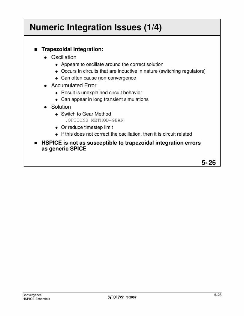
ConvergenceHSPICE Essentials
5-26© 2007
265-
Numeric Integration Issues (1/4)
� Trapezoidal Integration:
� Oscillation
� Appears to oscillate around the correct solution
� Occurs in circuits that are inductive in nature (switching regulators)
� Can often cause non-convergence
� Accumulated Error
� Result is unexplained circuit behavior
� Can appear in long transient simulations
� Solution
� Switch to Gear Method
.OPTIONS METHOD=GEAR
� Or reduce timestep limit
� If this does not correct the oscillation, then it is circuit related
� HSPICE is not as susceptible to trapezoidal integration errors as generic SPICE

ConvergenceHSPICE Essentials
5-27© 2007
275-
Numeric Integration Issues (2/4)
� Issues in GEAR integration:
� Large amounts of local truncation error
� Unexplainable simulation behavior
� Overshoot at transition points
� Solutions
� Reduce the maximum timestep
– Smaller TSTEP in .TRAN
– .OPTION DELMAX
� Switch to trapezoidal method
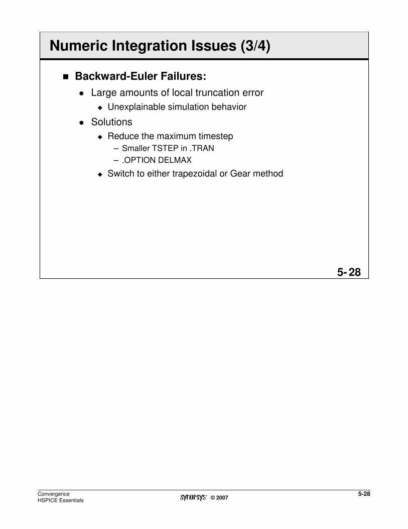
ConvergenceHSPICE Essentials
5-28© 2007
285-
Numeric Integration Issues (3/4)
� Backward-Euler Failures:
� Large amounts of local truncation error
� Unexplainable simulation behavior
� Solutions
� Reduce the maximum timestep
– Smaller TSTEP in .TRAN
– .OPTION DELMAX
� Switch to either trapezoidal or Gear method

ConvergenceHSPICE Essentials
5-29© 2007
295-
Numeric Integration Issues (4/4)
� Some cautions about using .OPTION DELMAX:
� If the problem is a model discontinuity, a small DELMAX will increase the likelihood of landing on it
� DELMAX can increase simulation time dramatically
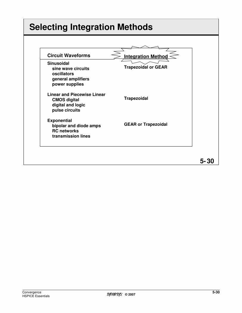
ConvergenceHSPICE Essentials
5-30© 2007
305-
Selecting Integration Methods
Circuit Waveforms
Sinusoidal
sine wave circuitsoscillators
general amplifierspower supplies
Linear and Piecewise Linear
CMOS digitaldigital and logic
pulse circuits
Exponential
bipolar and diode ampsRC networks
transmission lines
Integration Method
Trapezoidal or GEAR
Trapezoidal
GEAR or Trapezoidal

ConvergenceHSPICE Essentials
5-31© 2007
315-
Numeric Integration Comparisons (1/3)
Accumulated Error
BackwardsEuler
Trapezoidal
Oscillator - Backwards Euler Error vs. Trapezoidal (no error)
Volts
Time
2.0k
0
-2.0k
2.0k
0
-2.0k
0 5.0 10.0 15.0 20.0 25.0

ConvergenceHSPICE Essentials
5-32© 2007
325-
Numeric Integration Comparisons (2/3)
Trapezoidal vs. GEAR (overshoot)
Capacitor Test - Trapezoidal vs. Gear (overshoot)
GEAR
Amps
4.0p
3.0p
2.0p
1.0p
0
4.0p
3.0p
2.0p
1.0p
0
10.0M 200M 400M 600M 800M 1.0 1.2 1.4
10.0M 200M 400M 600M 800M 1.0 1.2 1.4
Time
TRAP

ConvergenceHSPICE Essentials
5-33© 2007
335-
Numeric Integration Comparisons (3/3)
Comparison: HSPICE vs. SPICE 2G.6
Capacitor - HSPICE Trapezoidal
Amps
Time
3.0p
2.0p
1.0p
0
0 500M 1.0 1.5 2.0
HSPICE
SPICE 2G.6
Trapezoidal
Oscillation

ConvergenceHSPICE Essentials
5-34© 2007
345-
LAB 5: HSPICE Converges
During this lab, you will examine how HSPICE converges to a transient solution.
HSPICE
Converges
Transient solution
45 minutes

Advanced Input ElementsHSPICE Essentials
6-1© 2007
16-
Agenda
© 2007 Synopsys, Inc. All Rights Reserved
DAY
2222Convergence5
Advanced Input Elements6
Customer SupportCS
Synopsys 60-I-031-BSG-008
Advanced Input ElementsHSPICE Essentials
6-2© 2007
26-
Unit Objectives
After completing this unit, you should be able to:
� Use parameter statements and functions
� Use .MEASURE statements to verify circuit specifications
� Use .ALTER blocks
� Use .BIASCHK to monitor element bias conditions

Advanced Input ElementsHSPICE Essentials
6-3© 2007
36-
Advanced Input File Elements
� Parameters
� Functions
� Algebraics
� .MEAS
� .ALTER
� .BIASCHK

Advanced Input ElementsHSPICE Essentials
6-4© 2007
46-
Parameters
� Syntax:
.PARAM parnam1=val1 <parnam2=val2...>
� Sets global values
� Parameterize input element, source, model data
� Algebraically manipulate output print/plot variables
� Central to circuit optimization and multiple simulation runs
Example:
.PARAM A=4 B=‘5*sqrt(A)’ C=10
R1 0 4 ‘C+5*A’

Advanced Input ElementsHSPICE Essentials
6-5© 2007
56-
Parameters: Rules (1/2)
� Top-Down Order:
� .OPTION PARHIER=GLOBAL
� Main Netlist .PARAM
� Subcircuit Call
� Subcircuit Definition
.subckt xin1 in out WW=80
M1 in out 0 0 mod W=WW
…
.ends
.param WW=100
X1 1 0 xin1 WW=90
Highest
Lowest

Advanced Input ElementsHSPICE Essentials
6-6© 2007
66-
Parameters: Rules (2/2)
Example:
.PARAM wp=50u lp=.6u ln=.6u abc=10
X1 1 2 inv wn=10u wp=20u ln=2u lp=.8u cba=5
.SUBCKT inv in out
+ wn=8u wp=8u ln=1u lp=1u abc=5
m1 out in vdd vdd p w=wp l=lp m=abc
m2 out in 0 0 n w=wn l=ln m=cba
.ENDS
� Actual Results:
� m1 l=.6u w=50u m=10
� m2 l=.6u w=10u m=5

Advanced Input ElementsHSPICE Essentials
6-7© 2007
76-
Using Parameters (1/2)
� .PARAMs are GLOBAL by default:
� Last definition at the main circuit level affects the entire netlist
� Set local scoping by using .options PARHIER=Local
� Not positional within the netlist
Example:
� Two libraries from two different manufacturers … lib1, lib2
� Each uses param ‘abc’ as a skew value
� Two different values for ‘abc’
� Lib1 will get the WRONG value for param ‘abc’
� Particularly dangerous when skew values are all read in as well as libs

Advanced Input ElementsHSPICE Essentials
6-8© 2007
86-
Using Parameters (2/2)
Example:
* In lib1
.lib tt
.param abc=0.9
.model nch.1 nmos level=1 vth=abc …
.endlib tt
*In lib2
.lib tt
.param abc=0.75
.model n.1 nmos level=1 vth=abc …
.endlib tt

Advanced Input ElementsHSPICE Essentials
6-9© 2007
96-
Parameters: Passing .IC to Subcircuits
� The ability to pass initial conditions to subcircuits is unique to HSPICE
� Application – Multi-stable circuits:
� Need state information to guide the DC solution
� Ring-oscillators, flip-flops must be initialized
Example:
.param vdd=5
Xflop1 in0 q0 q0bar d0 LATCH Q0set=Vdd
Xflop2 in1 q1 q1bar d1 LATCH Q1set=gnd
.SUBCKT LATCH in Q Qbar d Q0set=0 Q1set=Vdd
.ic v(Q0)=Q0set v(Q1)=Q1set
…
.ENDS

Advanced Input ElementsHSPICE Essentials
6-10© 2007
106-
Parameters: Flexibility and Productivity
� Parameters are integral to creating “Corner”Process Models:
� Fixed Model Lib with parameterized model parameters
� Easily change skew value by reassigning parameters
� Combine .param, .lib and/or .include

Advanced Input ElementsHSPICE Essentials
6-11© 2007
116-
Corner Process Model Example
* Netlist
R1 1 0 10k
.lib ‘MyProcess.lib TT
M1 1 1 2 0 nchan
.end
* MyProcess.lib file
.lib TT
* typical process
.param TOX_8=230 …
.include
+ ‘~/lib/cmos1.dat’
.endl TT
.lib FF
* fast process
.param TOX_8=200 …
.include
+ ‘~/lib/cmos1.dat’
.endl FF
* file: ~/lib/cmos1.dat
.model nchan
+ level=13 …
+ tox=tox_8

Advanced Input ElementsHSPICE Essentials
6-12© 2007
126-
Algebraics (1/2)
� Any parameter defined in the netlist can be replaced by an algebraic expression:
� Must be in quoted strings
� the assignment cannot contain output variables or dynamic simulation data
� Simple:
+, -, *, /
� Complex:
sin( ) sinh( ) cos( ) cosh( ) tan( )
tanh( ) atan( ) abs( ) min(x.x) max(x,x)
sqrt(x) exp(x) db(x) log(x) log10(x)
pwr(x,y) pow(x,y)
� These are available for use in algebraics:
time, hertz, temp

Advanced Input ElementsHSPICE Essentials
6-13© 2007
136-
Algebraics (2/2)
Examples:
.param x=‘y+3’
R1 1 0 r = ‘abs(v(1)/i(m1))/10’
� Apply to output variables as well:
.print dc v(3) v(2) gain=PAR(‘v(3)/v(2)’)
� Must enclose algebraic within quotes
� Continuation character for quoted strings is ‘\\’:
Example:
.param alf1(a,b,c)=‘(10*W*sqrt(a))+ \\
exp(b)*log(c)’
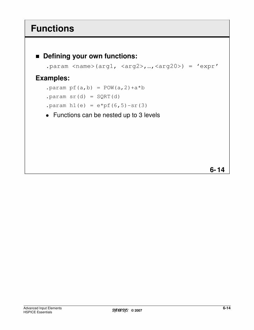
Advanced Input ElementsHSPICE Essentials
6-14© 2007
146-
Functions
� Defining your own functions:
.param <name>(arg1, <arg2>,…,<arg20>) = ‘expr’
Examples:
.param pf(a,b) = POW(a,2)+a*b
.param sr(d) = SQRT(d)
.param h1(e) = e*pf(6,5)-sr(3)
� Functions can be nested up to 3 levels
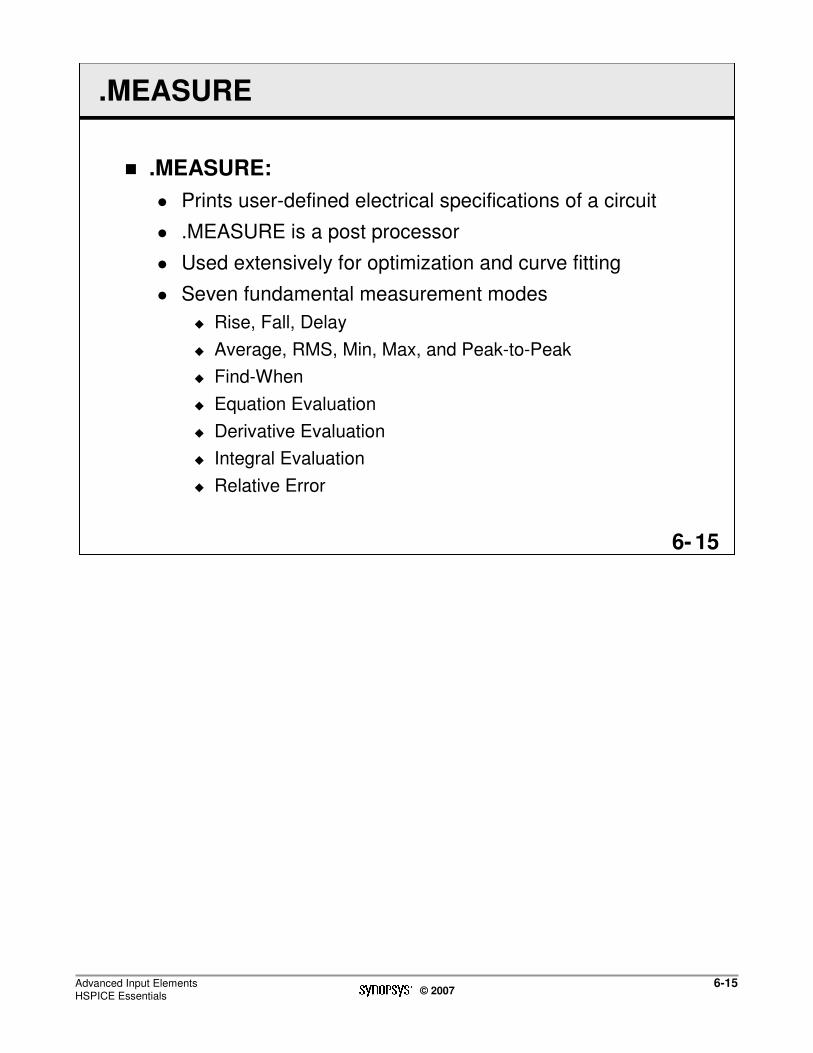
Advanced Input ElementsHSPICE Essentials
6-15© 2007
156-
.MEASURE
� .MEASURE:
� Prints user-defined electrical specifications of a circuit
� .MEASURE is a post processor
� Used extensively for optimization and curve fitting
� Seven fundamental measurement modes
� Rise, Fall, Delay
� Average, RMS, Min, Max, and Peak-to-Peak
� Find-When
� Equation Evaluation
� Derivative Evaluation
� Integral Evaluation
� Relative Error

Advanced Input ElementsHSPICE Essentials
6-16© 2007
166-
.MEASURE: Rise/Fall (1/2)
� Syntax:
.MEASURE <DC|TRAN|AC> result TRIG TARG
+ <optimization options>
� result - name given the measured value in the HSPICE output
TRIG trig_var VAL=trig_val <TD=timedelay>
+ <CROSS=#of> <RISE=#of> <FALL=#of>
TRIG AT=value
TARG targ_var VAL=targ_val <TD=timedelay>
+ <CROSS=#of|LAST><RISE=#of|LAST>
+ <FALLS=#of|LAST>

Advanced Input ElementsHSPICE Essentials
6-17© 2007
176-
.MEASURE: Rise/Fall (2/2)
Example:
.MEAS TRAN TDELAY TRIG V(1)
+ VAL=2.5 TD=10ns RISE=2
+ TARG V(2)VAL=2.5 FALL=2
Delay 10ns
…
…
2.5v
2.5v
TDLAY
V(1)
V(2)

Advanced Input ElementsHSPICE Essentials
6-18© 2007
186-
.MEASURE: AVG, RMS, MIN, MAX, PP (1/2)
� Syntax:
.MEASURE <DC|TRAN|AC> result func out_var
+ <FROM=val> <TO=val> <optimization options>
� Func
� AVG, RMS, MIN, MAX, PP
� Result
� Name given the measured value in the HSPICE output
� Out_var
� Name of the output variable to be measured

Advanced Input ElementsHSPICE Essentials
6-19© 2007
196-
.MEASURE: AVG, RMS, MIN, MAX, PP (2/2)
Examples:
.MEAS TRAN avgval AVG V(10)From=10ns To=55ns
� Print out average nodal voltage of node 10 during tran time 10 to 55ns
� Print as “avgval”
.MEAS TRAN maxval MAX V(1,2)
+ From=15ns To=100ns
� Find the maximum voltage difference between nodes 1 and 2 from time 15ns to 100ns
� Print as “maxval”

Advanced Input ElementsHSPICE Essentials
6-20© 2007
206-
.MEASURE: FIND-WHEN
� Allows any independent variables (time, frequency, parameter), by using WHEN syntax, or any dependent variables (voltage, current, etc), by using Find-When syntax, to be measured when some specific event occurs
� Syntax:
.MEASURE <DC|TRAN|AC> result WHEN out_var=val
+ <TD=val> <RISE=#of>|LAST> <FALL=#of|LAST>
+ <CROSS=#of|LAST> <optimization options>

Advanced Input ElementsHSPICE Essentials
6-21© 2007
216-
.MEASURE: FIND-WHEN Examples
Example of WHEN:
.MEAS TRAN fifth WHEN V(osc_out)=2.5v RISE=5
� Measure the time of the 5th rise of node “osc_out” at 2.5v
� Store in variable fifth
Example of FIND-WHEN:
.MEAS TRAN result FIND v(out) WHEN v(in)=40m
� Measure v(out) when v(in)=40m
� Store in variable result
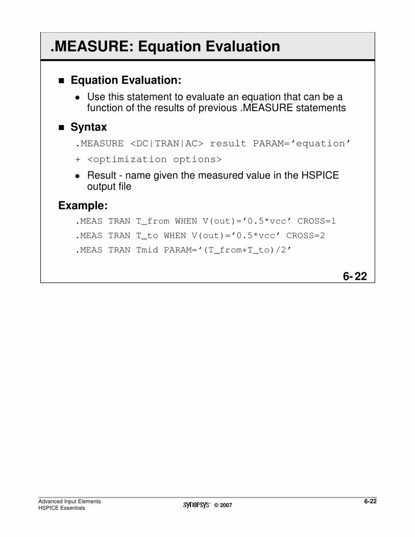
Advanced Input ElementsHSPICE Essentials
6-22© 2007
226-
.MEASURE: Equation Evaluation
� Equation Evaluation:
� Use this statement to evaluate an equation that can be a function of the results of previous .MEASURE statements
� Syntax
.MEASURE <DC|TRAN|AC> result PARAM=‘equation’
+ <optimization options>
� Result - name given the measured value in the HSPICE output file
Example:
.MEAS TRAN T_from WHEN V(out)=’0.5*vcc’ CROSS=1
.MEAS TRAN T_to WHEN V(out)=’0.5*vcc’ CROSS=2
.MEAS TRAN Tmid PARAM=‘(T_from+T_to)/2’

Advanced Input ElementsHSPICE Essentials
6-23© 2007
236-
.MEASURE: Derivative Function
� Derivative Function:
� Provides the derivative of an output variable at a given time or frequency or for any sweep variable
� Provides the derivative of a specified output variable when some specific event occurs
� Syntax:
.MEASURE <DC|TRAN|AC> result DERIVATIVE
+ out_var WHEN var2=val <TD=val>
+ <RISE=#of>|LAST> <FALL=#of|LAST>
+ <CROSS=#of|LAST> <optimization options>
Example:
.MEAS TRAN slewrate DERIV v(1)
+ WHEN V(osc_out)=2.5v RISE=5

Advanced Input ElementsHSPICE Essentials
6-24© 2007
246-
.MEASURE: Integral Function
� Integral Function:
� Provides the integral of an output variable over a specified period
� Syntax:
.MEASURE <DC|TRAN|AC> result INTEGRAL out_var
+ <FROM=val1> <TO=val2> <optimization options>
Example:
.MEAS TRAN charge INTEG I(cload)
+ FROM=10ns TO=100ns

Advanced Input ElementsHSPICE Essentials
6-25© 2007
256-
Standalone Measure Utility
� Allows the user to calculate new measure statements from the previous simulation results
� Supports
� *.ac#, *.sw# and *.tr# wave files
� ‘measurefile’ supports the following statements
� .measure, .temp, .data, .enddata, .param, .option, .end
� The variables of the .measure statements in the measure file should exist in the .tr#, ac# or .sw# file
� Syntax
hspice –meas <measurefile> -i <wavefile> -o <output>
� measurefile - File that contains .measure and other supported statements
� wavefile - .tr#, .ac# and .sw# file produced by HSPICE
� output - Measurement results
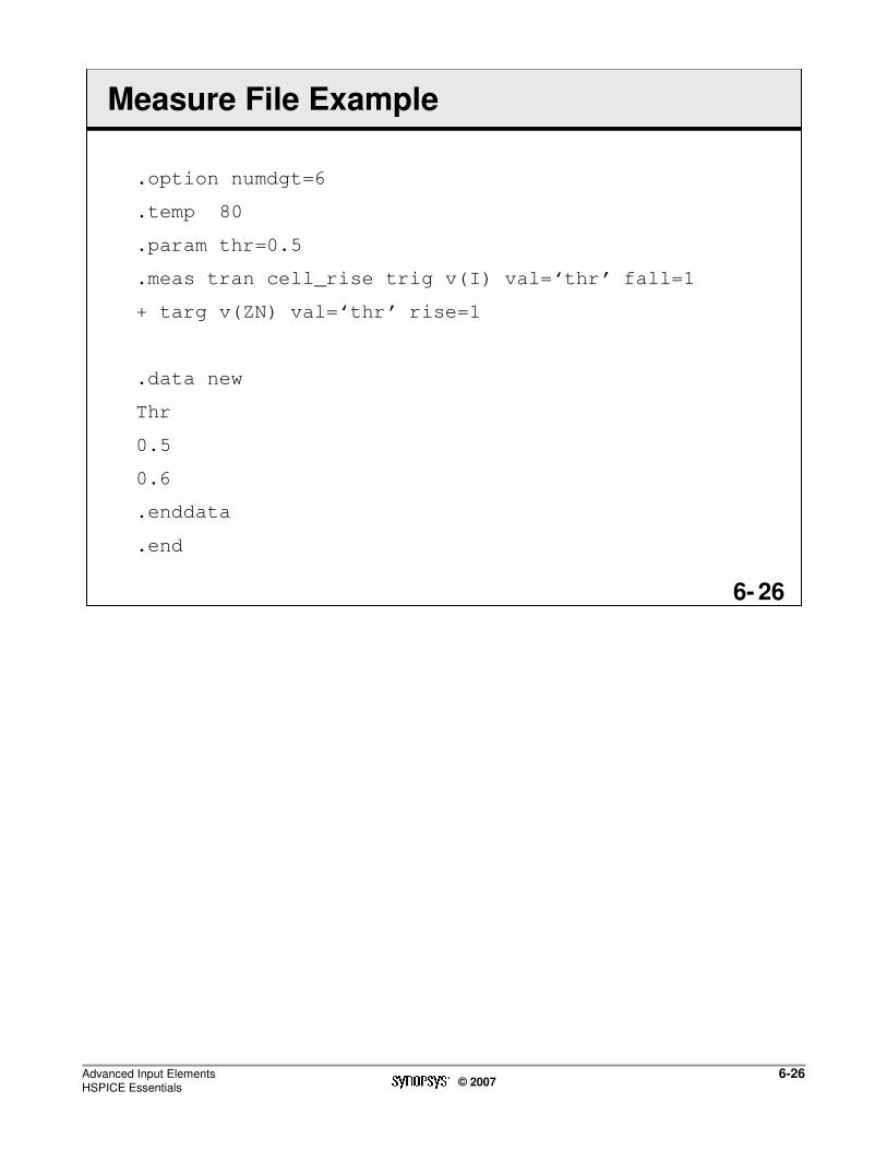
Advanced Input ElementsHSPICE Essentials
6-26© 2007
266-
Measure File Example
.option numdgt=6
.temp 80
.param thr=0.5
.meas tran cell_rise trig v(I) val=‘thr’ fall=1
+ targ v(ZN) val=‘thr’ rise=1
.data new
Thr
0.5
0.6
.enddata
.end

Advanced Input ElementsHSPICE Essentials
6-27© 2007
276-
.ALTER: Description
� Rerun a simulation several times with different:
� Circuit topology
� Models
� Library components
� Elements
� Parameter values
� Options
� Source stimulus
� Analysis variables
� Print/probe commands
� Must be parameterized

Advanced Input ElementsHSPICE Essentials
6-28© 2007
286-
.ALTER: Limitations
� CAN include:
� Element Statements
� .DATA, .LIB, .DEL LIB, .INCLUDE, .MODEL statements
� .IC, .NODESET statements
� .OP, .OPTIONS, .PARAM, .TEMP, .TF, .TRAN, .DC, .AC
� CANNOT include:
� .PRINT, .PROBE, or any other i/o statements
� Unless they are parameterized
� AVOID:
� Adding analysis statements under each .ALTER block
� Will cause huge penalty in simulation time and confusion in the output results

Advanced Input ElementsHSPICE Essentials
6-29© 2007
296-
.ALTER: .option ALTCC (1/2)
� Enables HSPICE to read netlist only once under multiple .ALTER statements
� Syntax
.option ALTCC<=x>
� Where
� x=1 - Enabled
� x=0 - Disabled (default)

Advanced Input ElementsHSPICE Essentials
6-30© 2007
306-
.ALTER: .option ALTCC (2/2)
� Supported statements in .ALTER block
� Passive elements (e.g. R, C, L)
� Sources (e.g. V, I, E, F)
� .PARAM
� .DATA/.ENDDATA
� Analysis statement (e.g. .DC, .TRAN, .AC)
� .TEMP
� .MEAS
� .TITLE

Advanced Input ElementsHSPICE Essentials
6-31© 2007
316-
.ALTER: Example
* ALTER Test
* CMOS Inverter
.OPTIONS ACCT LIST
.OP
.DC VIN 0 5 0.1
.PRINT DC v(3) v(2)
.PRINT tran v(3)
.PARAM VDD=5
.LIB ‘MOS.LIB’ NORMAL
VDD 1 0 VDD
VIN 2 0
M1 3 2 1 1 P 6U 15U
M2 3 2 0 0 N 6U 15U
.ALTER Change Supply
.PARAM VDD=10
.ALTER Fast Process
.DEL LIB ‘MOS.LIB’ NORMAL
.LIB ‘MOS.LIB’ FAST
.ALTER Add Transient
.TRAN .1 2
.END
alter to add transient(VDD=10v still in effect)(.lib ‘mos.lib’ FAST still in effect).OPDC SweepTransient
.OPDC Sweep
change VDD to 10v.OPDC Sweep
alter change to fast library (MUST delete first)(VDD=10v still in effect).OPDC Sweep

Advanced Input ElementsHSPICE Essentials
6-32© 2007
326-
Worst Case Analysis (1/2)
� Worst case corners analysis
� Component value limits are known, measured, and implemented as skew parameters
� Simple, fast check of a design at process limits
� Tends to be overly pessimistic
� Done through best, worst case model selection
� Simple Worst Case Analysis:
� Switch to different process corner libraries and repeat simulation
� .ALTER, .DEL LIB, .LIB
Example:.LIB ‘CMOS.lib’ SLOW
.Tran …
.ALTER Run Fast Corner Library
.DEL LIB ‘CMOS.lib’ SLOW
.LIB ‘CMOS.lib’ FAST
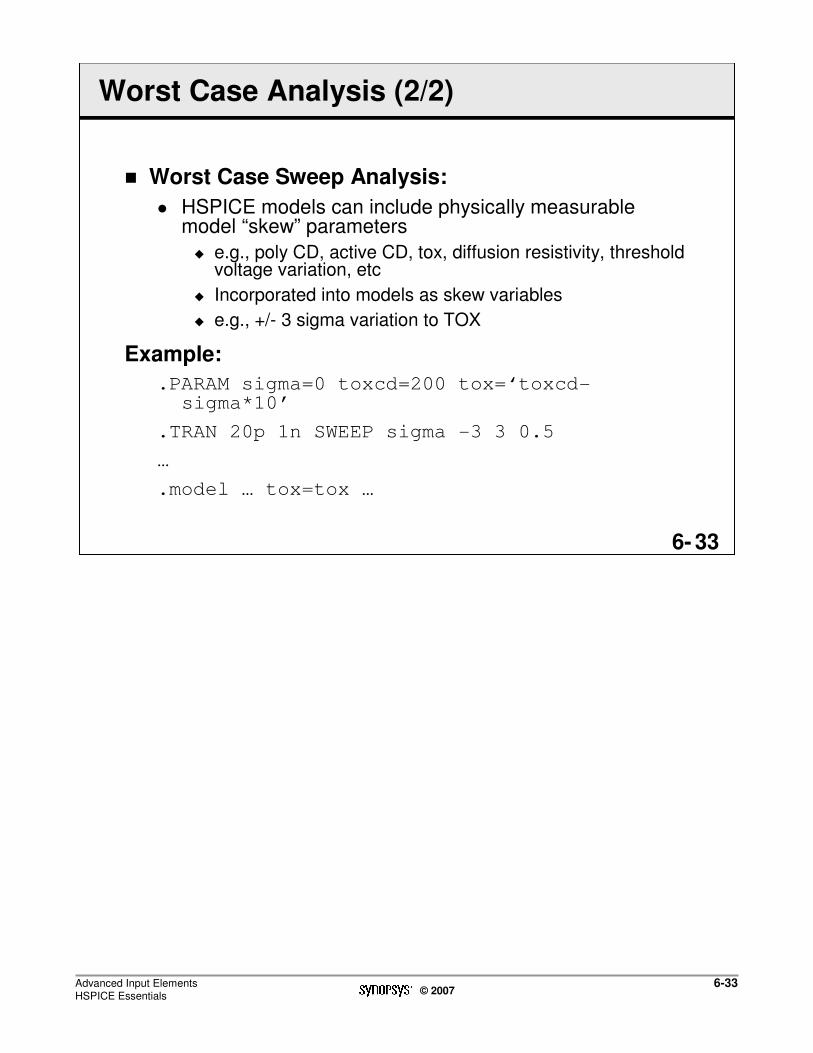
Advanced Input ElementsHSPICE Essentials
6-33© 2007
336-
Worst Case Analysis (2/2)
� Worst Case Sweep Analysis:
� HSPICE models can include physically measurable model “skew” parameters
� e.g., poly CD, active CD, tox, diffusion resistivity, threshold voltage variation, etc
� Incorporated into models as skew variables
� e.g., +/- 3 sigma variation to TOX
Example:
.PARAM sigma=0 toxcd=200 tox=‘toxcd-sigma*10’
.TRAN 20p 1n SWEEP sigma -3 3 0.5
…
.model … tox=tox …
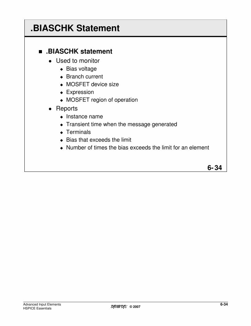
Advanced Input ElementsHSPICE Essentials
6-34© 2007
346-
.BIASCHK Statement
� .BIASCHK statement
� Used to monitor
� Bias voltage
� Branch current
� MOSFET device size
� Expression
� MOSFET region of operation
� Reports
� Instance name
� Transient time when the message generated
� Terminals
� Bias that exceeds the limit
� Number of times the bias exceeds the limit for an element

Advanced Input ElementsHSPICE Essentials
6-35© 2007
356-
.BIASCHK Options
� Option BIASFILE and Option BIAWARN direct the flow of BIASCHK messages
� .OPTION BIASFILE = ‘filename’
� HSPICE outputs the results of all .BIASCHK messages to a file that you specify
� .OPTION BIAWARN = 0 | 1
� Set to 1, HSPICE reports BIASCHK messages during transient analysis to standard output and in output listing file after transient
� Set to 0 (default), HSPICE report BIASCHK messages to output listing file only

Advanced Input ElementsHSPICE Essentials
6-36© 2007
366-
.BIASCHK Keywords (1/3)
� type
� MOS, NMOS, PMOS, JFET, BJT, DIODE, C, SUBCKT
� terminal1, terminal2
� Terminals to check bias between
� MOS level 57: nd, ng, ns, ne, np, nb
� MOS level 58: nd, ngf, ns, ngb
� MOS level 59: nd, ng, ns, ne, np
� all other MOS levels: nd, ng, ns, nb
� capacitor: n1, n2
� diode: np, nn
� bipolar: nc, nb, ne, ns
� JFET: nd, ng, ns, nb
� SUBCKT: the pins defined by the subcircuit
� limit
� Threshold when BIASCHK issue warning
� noise
� Threshold tolerance
� Default is 0.1v
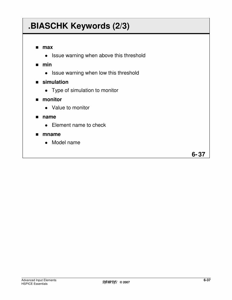
Advanced Input ElementsHSPICE Essentials
6-37© 2007
376-
.BIASCHK Keywords (2/3)
� max
� Issue warning when above this threshold
� min
� Issue warning when low this threshold
� simulation
� Type of simulation to monitor
� monitor
� Value to monitor
� name
� Element name to check
� mname
� Model name

Advanced Input ElementsHSPICE Essentials
6-38© 2007
386-
.BIASCHK Keywords (3/3)
� tstart
� Start time during transient analysis
� Default is 0
� tstop
� End time during transient analysis
� Default is the stop time of the transient analysis
� autostop
� Report error messages and stop the simulation immediately
� except
� Do not perform bias check on specified elements or instances
� region
� MOSFET operating region

Advanced Input ElementsHSPICE Essentials
6-39© 2007
396-
.BIASCHK Element and Model Monitor Syntax
.BIASCHK type terminal1=t1 <terminal2=t2>
+ <limit=lim> <noise=ns> <max=max> <min=min>
+ <simulation=op|dc|tr|all> <monitor=v|i>
+ <name=name1,name2, ...>
+ <mname=modname_1,modname_2, ...>
+ <tstart=time1> <tstop=time2> <autostop>
+ <except=name1,name2, ...>
Examples:
.BIASCHK NMOS terminal1=ng terminal2=nb limit=2v
+ noise=0.01v name=x1.x3.m1 mname=nch name=m3
.BIASCHK DIODE terminal1=np terminal2=nn
+ max=.006 name=d1, d2

Advanced Input ElementsHSPICE Essentials
6-40© 2007
406-
.BIASCHK Expression Monitor Syntax
.BIASCHK ‘expression’
+ <limit=lim> <noise=ns> <max=max> <min=min>
+ <simulation=op|dc|tr|all>
+ <monitor=v|i>
+ <tstart=time1> <tstop=time2> <autostop>
Examples:
.BIASCHK 'v(out)/v(in)' min=.01 max=10
+ simulation=tr
.BIASCHK 'v(1)' min = 'v(2)*2' simulation= op

Advanced Input ElementsHSPICE Essentials
6-41© 2007
416-
.BIASCHK MOS Region Monitor Syntax
� Region monitor only applies to type MOS
.BIASCHK MOS
+ <region=cutoff|linear|saturation>
+ <name=name1,name2, ...>
+ <mname=modname_1,modname_2, ...>
+ <tstart=time1> <tstop=time2> <autostop>
+ <except=name1,name2, ...>
Example:
.BIASCHK MOS region=saturation
+ name=x1.m1 mname=nch name=m2
.BIASCHK MOS region=cutoff
+ name=x2.m*

Advanced Input ElementsHSPICE Essentials
6-42© 2007
426-
.BIASCHK MOS Device Size Monitor Syntax
� Only W and L of type MOS, NMOS, PMOS can be monitored
.BIASCHK type
+ <limit=lim> <noise=ns> <max=max> <min=min>
+ <simulation=op|dc|tr|all> <monitor=w|l>
+ <name=name1,name2, ...>
+ <mname=modname_1,modname_2, ...>
+ <tstart=time1> <tstop=time2> <autostop>
+ <except=name1,name2, ...>
Example:
.BIASCHK MOS monitor = l mname=n* mname=p*
+ min = 1u simulation=op

Advanced Input ElementsHSPICE Essentials
6-43© 2007
436-
.BIASCHK Report – Minimum Bias Value (1/2)
Biaschk output during transient analysis:
type terminals time Val_chk method model-name element-name
mos v(nd-ns) 0. -4.5151n min p xbuf.x1.mp1
mos v(nd-ns) 0. 2.6877n min n xbuf.x10.mn1
mos v(nd-ns) 0. -4.5151n min p xbuf.x2.mp1
mos v(nd-ns) 500.0000p -4.5151n min p xbuf.x1.mp1
mos v(nd-ns) 500.0000p 2.6877n min n xbuf.x10.mn1
mos v(nd-ns) 500.0000p -4.5151n min p xbuf.x2.mp1
mos v(nd-ns) 600.0000p -8.0780u min p xbuf.x2.mp1
mos v(nd-ns) 10.9500n 8.8781u min p xbuf.x10.mp1
mos v(nd-ns) 10.9500n 7.5221u min p xbuf.x12.mp1
mos v(nd-ns) 10.9500n -534.7583n min n xbuf.x2.mn1
mos v(nd-ns) 10.9500n -3.3000 min p xbuf.x2.mp1
mos v(nd-ns) 20.7500n -534.7583n min n xbuf.x2.mn1
mos v(nd-ns) 20.7500n -3.3000 min p xbuf.x2.mp1
mos v(nd-ns) 20.9000n 1.3155u min n xbuf.x1.mn1
mos v(nd-ns) 180.9000n 3.2672u min n xbuf.x10.mn1
mos v(nd-ns) 200.0000n -3.3043u min p xbuf.x1.mp1
mos v(nd-ns) 200.0000n 3.2672u min n xbuf.x10.mn1
mos v(nd-ns) 200.0000n -3.3000 min p xbuf.x10.mp1
mos v(nd-ns) 200.0000n 5.6830u min p xbuf.x11.mp1
mos v(nd-ns) 200.0000n -2.0859u min p xbuf.x2.mp1
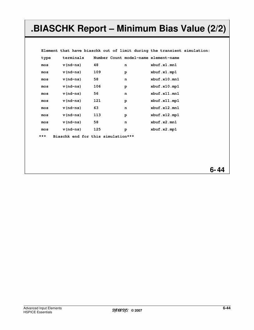
Advanced Input ElementsHSPICE Essentials
6-44© 2007
446-
.BIASCHK Report – Minimum Bias Value (2/2)
Element that have biaschk out of limit during the transient simulation:
type terminals Number Count model-name element-name
mos v(nd-ns) 48 n xbuf.x1.mn1
mos v(nd-ns) 109 p xbuf.x1.mp1
mos v(nd-ns) 58 n xbuf.x10.mn1
mos v(nd-ns) 106 p xbuf.x10.mp1
mos v(nd-ns) 56 n xbuf.x11.mn1
mos v(nd-ns) 121 p xbuf.x11.mp1
mos v(nd-ns) 63 n xbuf.x12.mn1
mos v(nd-ns) 113 p xbuf.x12.mp1
mos v(nd-ns) 58 n xbuf.x2.mn1
mos v(nd-ns) 125 p xbuf.x2.mp1
*** Biaschk end for this simulation***

Advanced Input ElementsHSPICE Essentials
6-45© 2007
456-
Lab 6: Advanced Input File Elements
During this lab you will use:
1. .measure commands to verify design specifications.
2. .alter statements to repeat simulations
3. .biaschk statements
Measure commands
Verify Specifications
.alter statements
.biaschk statements
45 minutes

Advanced Input ElementsHSPICE Essentials
6-46© 2007
This page was intentionally left blank.

Customer Support CS-1© 2007
Customer Support
© 2007 Synopsys, Inc. All Rights Reserved 20070822

Customer Support CS-2© 2007
2CS-
Synopsys Support Resources
1. Build Your Expertise: Customer Education Services� www.synopsys.com/support
� Workshop schedule and registration
� Download materials(SolvNet id required)
2. Empower Yourself: solvnet.synopsys.com
� Online technical information and access to support resources
� Documentation & Media
3. Access Synopsys Experts: Support Center

Customer Support CS-3© 2007
3CS-
� Immediate access to the latest technical information
� Product- and Release-Specific Update Training
� Thousands of expert-authored articles, Q&As, scripts and tool tips
� Enter-a-call online Support Center access
� Release information
� Online documentation
� License keys
� Electronic software downloads
� Synopsys announcements (latest tool, event and product information)
SolvNet Online Support Offers
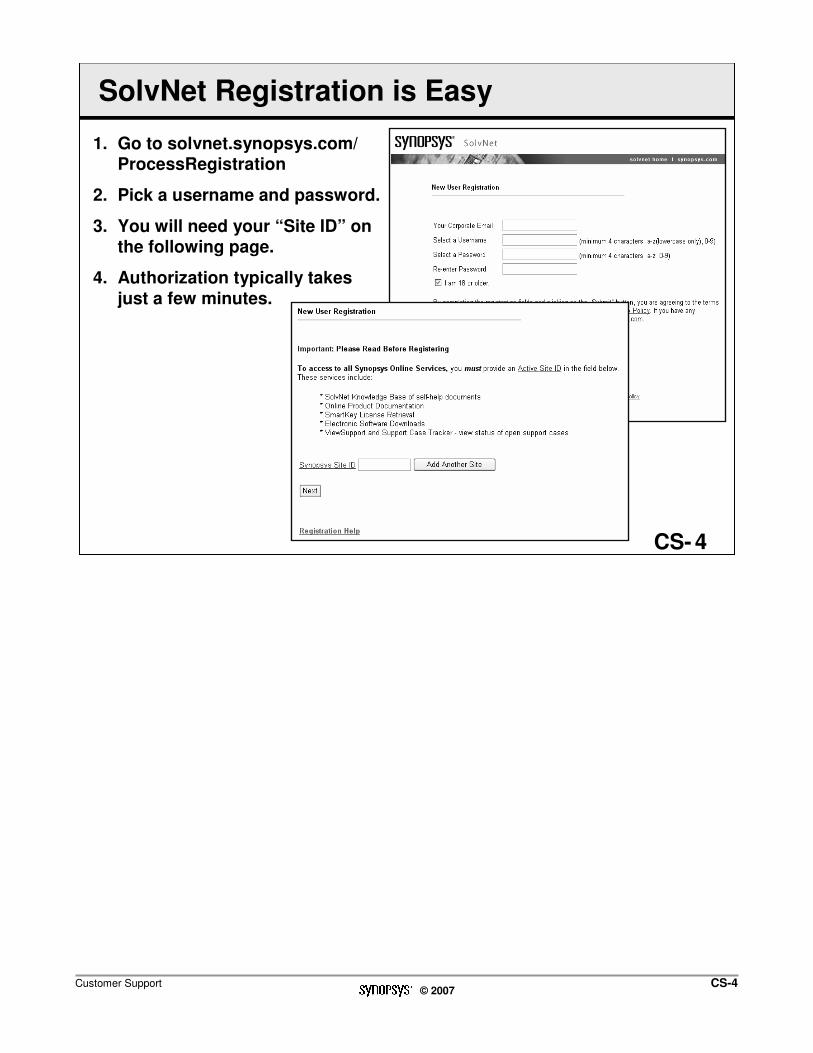
Customer Support CS-4© 2007
4CS-
SolvNet Registration is Easy
1. Go to solvnet.synopsys.com/ ProcessRegistration
2. Pick a username and password.
3. You will need your “Site ID” on the following page.
4. Authorization typically takes
just a few minutes.
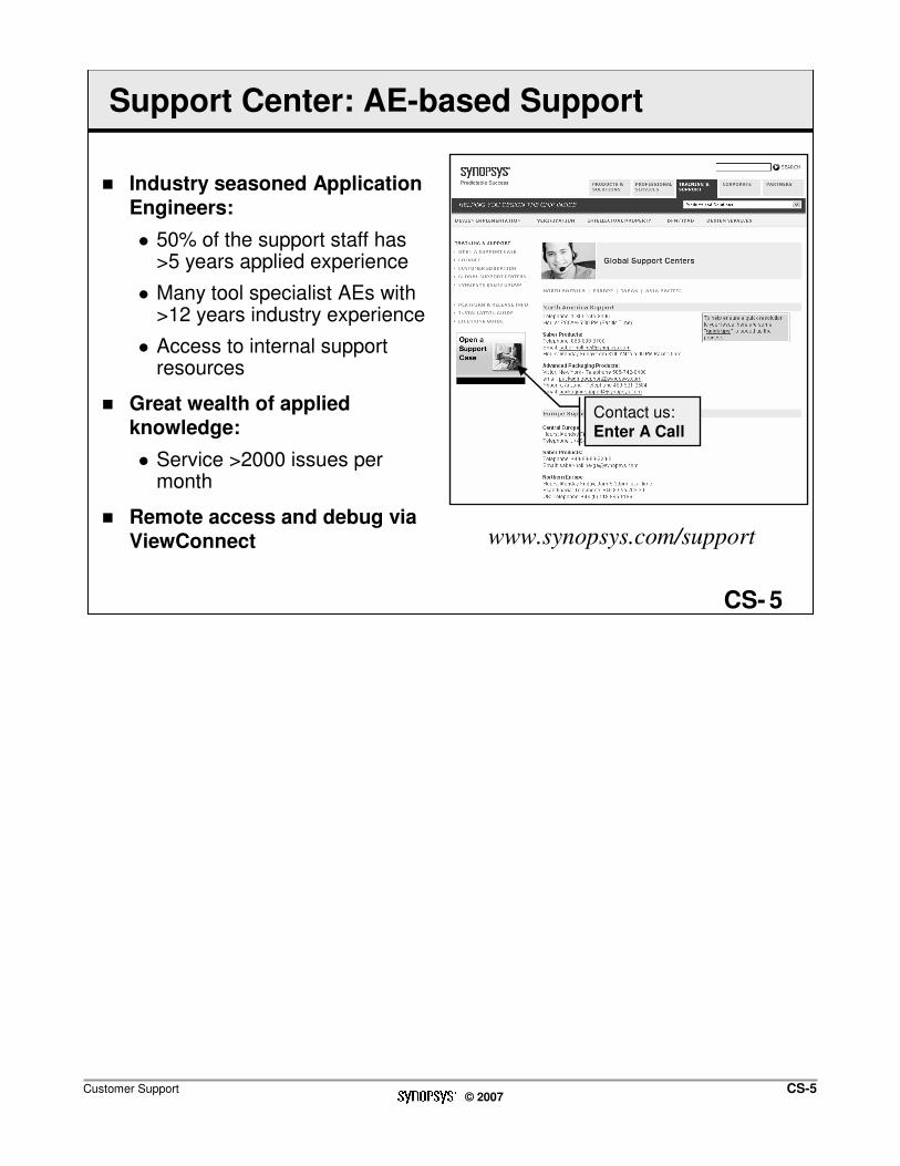
Customer Support CS-5© 2007
5CS-
Support Center: AE-based Support
� Industry seasoned Application Engineers:
� 50% of the support staff has >5 years applied experience
� Many tool specialist AEs with >12 years industry experience
� Access to internal support resources
� Great wealth of applied knowledge:
� Service >2000 issues per month
� Remote access and debug via ViewConnect
Contact us: Enter A Call
www.synopsys.com/support

Customer Support CS-6© 2007
6CS-
Other Technical Sources
� Application Consultants (ACs):
� Tool and methodology pre-sales support
� Contact your Sales Account Manager for more information
� Synopsys Professional Services (SPS) Consultants:
� Available for in-depth, on-site, dedicated, custom consulting
� Contact your Sales Account Manager for more details
� SNUG (Synopsys Users Group):
� www.snug-universal.org

Customer Support CS-7© 2007
7CS-
Summary: Getting Support
� Customer Education Services
� SolvNet
� Support Center
� SNUG

Customer Support CS-8© 2007
This page was intentionally left blank.