hydraulic analysis of surcharged storm sewer systems
TRANSCRIPT

University of KentuckyUKnowledge
KWRRI Research Reports Kentucky Water Resources Research Institute
3-1983
Hydraulic Analysis of Surcharged Storm SewerSystemsDigital Object Identifier: https://doi.org/10.13023/kwrri.rr.137
Don J. WoodUniversity of Kentucky
Gregory C. HeitzmanUniversity of Kentucky
Click here to let us know how access to this document benefits you.
Follow this and additional works at: https://uknowledge.uky.edu/kwrri_reports
Part of the Hydraulic Engineering Commons, Natural Resources Management and PolicyCommons, and the Water Resource Management Commons
This Report is brought to you for free and open access by the Kentucky Water Resources Research Institute at UKnowledge. It has been accepted forinclusion in KWRRI Research Reports by an authorized administrator of UKnowledge. For more information, please [email protected].
Repository CitationWood, Don J. and Heitzman, Gregory C., "Hydraulic Analysis of Surcharged Storm Sewer Systems" (1983). KWRRI Research Reports.66.https://uknowledge.uky.edu/kwrri_reports/66

Research Report No. 137
HYDRAULIC ANALYSIS OF SURCHARGED STORM SEWER SYSTEMS
By
Dr. Don J. Wood
Principal Investigator
and
Gregory C. Heitzman
Graduate Assistant
Project Number: A-084-KY (Completion Report)
Agreement Numbers: 14-34-0001-1119 (FY 19811 14-34-0001-2119 (FY 1982)
Period of Project: October 1980 - March 1983
University of Kentucky Water Resources Research Institute
Lexington, Kentucky
The work upon which this report is based was supported in part by funds provided by the United States Department of the Interior, Washington, D.C., as authorized by the Water Research and Development Act of 1978. Public Law 95-467.
March 1983

DISCLAIMER
Contents of this report do not necessarily reflect the views and policies of the United States Department of the Interior, Washington, D.C., nor does the mention of trade names or commercial products constitute their endorsement or recommendation for use by the U.S. Govermnent.
i
ABSTRACT
HYDRAULIC ANALYSIS OF SURCHARGED STORM SEWER SYSTEMS
Surcharge in a storm sewer system is the condition in which an entire sewer section is submerged and the pipe is flowing full under pressure. Flow in a surcharged storm sewer is essentially slowly varying unsteady pipe flow and methods for analyzing this type of flow are investigated. In this report the governing equations for unsteady fluid flow in pressurized storm sewers are presented. From these governing equations three numerical models are developed using various assumptions and simplifications. These flow models are applied to several example storm sewer systems under surcharge conditions. Plots of hydraulic grade and flow throughout the sewer network are presented in order to evaluate the ability of each model to accurately analyze surcharged storm sewer systems. Computer programs are developed for each of the models consi-· dered and these programs are presented and documented in the Appendix of this report.
Descriptors: storm sewer, surcharged, pressurized, unsteady, transient
ii
ACKNOWLEDGEMENTS
This work was supported by a grant from the Kentucky Water Resources Research Institute under project A-084-KY and a grant from the United States Department of the Interior, Washington, D.C. Gregory Heitzman served as a graduate assistant on this project and provided many valuable contributions to the effort.
iii
TABLE OF CONTENTS
DISCLAIMER
ABSTRACT.
ACKNOWLEDGEMENTS
LIST OF ILLUSTRATIONS.
LIST OF TABLES •
l - INTRODUCTION
2 - REVIEW OF EXISTING STORM SEWER WORK.
2.1 Pressurized Flow Models •••• 2.2 Surcharge Storm Sewer Flow Models 2.3 Other Related Surcharge Work.
3 - THEORY OF ONE DIMENSIONAL UNSTEADY FLOW.
3.1 Equation of Continuity (Mass Conservation). 3.2 Equation of Motion (Momentum) ••••••• 3.3 Governing Equations for Unsteady Surcharged
Sewer Flow. • • • • • . • • • 3.4 Classification of Pressurized Storm Sewer Flow.
4 - PRESSURIZED STORM SEWER SYSTEMS MODELS
4.1 Finite Element Method •••••• 4.2 Dynamic Lumped Parameter Method • 4.3 Kinematic Method (Steady State with Storage). 4.4 System Boundary Conditions ••••• 4.5 Initial Conditions ••••••••• 4.6 System Equation Assembly and Assumptions.
5 - EXAMPLE PROBLEMS AND RESULTS
5.1 Example Problem #1. 5.2 Example Problem #2. 5.3 Example Problem #3. 5.4 Example Problem #4. 5.5 Example Problem #5.
6 - CONCLUSIONS AND RECOMMENDATIONS.
6.1 Finite Element Model. 6.2 Dynamic Model. 6.3 Kinematic Model •••
iv
Page
i
ii
iii
vi
viii
1
5
5 6 8
10
10 19
24 25
28
28 39 43 46 51 51
. 54
54 60 66 75 85
95
95 98 99
7 - COMPUTER PROGRAMS • • •
7.1 Fortran Programs. 7.2 Data Coding Instructions.
APPENDICES • . •
Appendix A - FESSA Program Listing Appendix B - DYN/KIN Program Listing
REFERENCES . . . . . . . . . . . . . .
v
101
101 102
111
111 129
139

LIST OF ILLUSTRATIONS
FIGURE PAGE
2-1 Priessmann Slot Technique • • • • • • • • • • • • • • • • • 7
3-1 Application of Control Volume for Continuity Equation • • 11
3-2 Stresses and Strains Shown Acting on a Pipe Wall • • 14
3-3 Pipeline Constraint Conditions • • • • . • • • • • • 15
3-4 Free Body Diagram for the Momentum Equation • • • • . • • • 19
3-5 Force Balance on a Pipe . • • • • . • • . . • • • • • 21
4-1 Smooth Curve Approximation by Linear Elements • • • • 30
4-2 A Single Linear, Element Approximation • • • • • 31
4-3 Time Shape and Weighting Functions • • • • • • 36
4-4 Rigid Fluid Column • • • . • • • • • • • • • • • 43
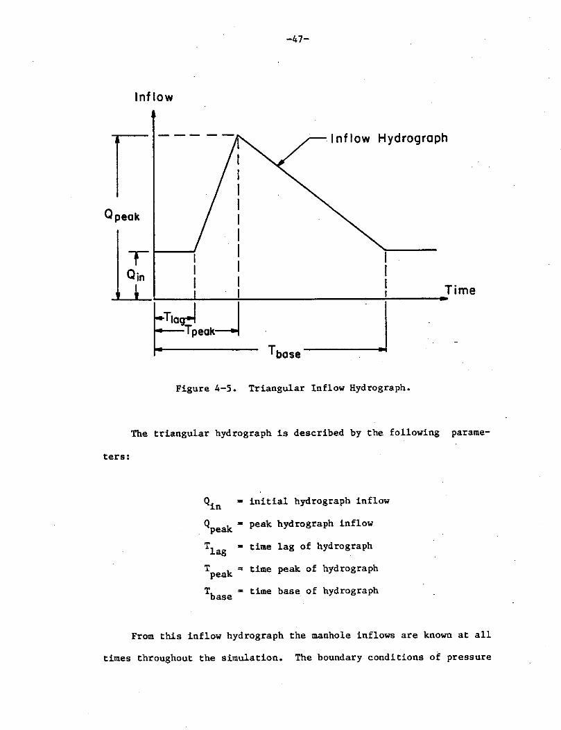
4-5 Triangular Inflow Hydrograph • • • • • • • • • 47
4-6 Manhole (Junction) Boundary Conditions • • • • • • • • 49
4-7 Flooded Manhole Conditions • • • . • • • • • • so
5-1 One Pipe Sewer System, Example II 1 • • • • • • • 56
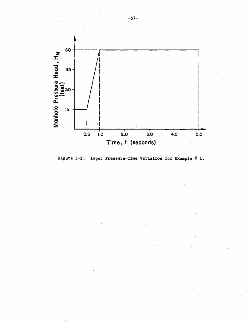
5-2 Input Pressure-Time Variation for Example II 1 • • • • 57
5-3 Total Head Graph for Junction 1 • • • • • 58
5-4 Flow Graph for Pipe 1 • • • • • • • • • • • • 59
s-s One Pipe sewer System, Example Problem# 2 • • • • 62
5-6 Inflow Hydrograph Corresponding to Table 5-2 • • • • • 62
5-7 Head and Flow Graphs for Junction 1 and Pipe 1, Example 2a 63
5-8 Head and Flow Graphs for Junction 1 and Pipe 1. Example 2b 64
5-9 Head and Flow Graphs for Junction 1 and Pipe 1, Example 2c 65
5-10 Five Pipe Sewer System, Example II 3 • . • • . . . . • • • . 69
vi
FIGURE PAGE
5-11 Head and Flow Graphs for Junction 1 and Pipe 1. Example II 3 70
5-12 Head and Flow Graphs for Junction 2 and Pipe 2, Example II 3 71
5-13 Head and Flow Graphs for Junction 3 and Pipe 3, Example II 3 72
5-14 Head and Flow Graphs for Junction 4 and Pipe 4, Example II 3 73
5-15 Head and Flow Graphs for Junction 5 and pipe 5, Example II 3 74
5-16 Seven Pipe Sewer System, Example II 4 • • . • • • • • . • • 77
5-17 Head and Flow Graphs for Junction 1 and Pipe 1. Example II 4 78
5-18 Head and Flow Graphs for Junction 2 and Pipe 2, Example # 4 79
5-19 Head and Flow Graphs for Junction 3 and Pipe 3, Example II 4 80
5-20 Head and Flow Graphs for Junction 4 and Pipe 4, Example II 4 81
5-21 Head and Flow Graphs for Junction 5 and pipe 5, Example II 4 82
5-22 Head and Flow Graphs for Junction 6 and Pipe 6, Example II 4 83
5-23 Head and Flow Graphs for Junction 7 and pipe 7, Example II 4 84
5-24 Three Pipe Sewer System, Example II 5 • • . • • • • 88
5-25 Total Head Graph for Junction 1, Example II 5 • • • • • 89
5-26 Flow Graph for Pipe 1, Example II 5 . . . . • • • 90
5-27 Total Head Graph for Junction 2, Example II 5 • 91
5-28 Flow Graph for Pipe 2, Example II 5 • • • • . • • • • • 92
5-29 Total Head Graph for Junction 3, example II 5 • • • • 93
5-30 Flow Graph for Pipe 3, Example II 5 . • . • • • 94
vii
LIST OF TABLES
TABLE PAGE
5-1 Sewer System Properties for Example II 2 • • • • • • 61
5-2 Hydrograph Properties for Example II 2 • • • • • • • 61
5-3 Sewer System Properties for Example fl 3 • • • • • • • • 68
5-4 Sewer System Properties for Example fl 4 • • • • • • • • 76
5-5 Sewer System Properties for Example fl 5 • • • • • • • 87
7-1 Data Coding Instruct ions for FESSA Fortran Program • • • • 103
7-2 Data Coding Instructions for DYN/KIN Fortran Program • • • 104
7-3 Example FESSA Data Coding for Example fl 3 • • • • • • • • • 105
7-4 Example DYN/KIN Data Coding for Example II 3 • • • • • • • • 106
7-5 Example FESSA Solution Results for Example# 3 • • • • • • 107
7-6 Example DYN/KIN Solution Results for Example # 3 • • • . 109
viii
INTRODUCTION
A storm sewer system is characterized by a series of manholes or
junctions (nodes) which are connected by sewer pipes (links) to form
a network. Manholes serve two main purposes in drainage systems.
They provide access to the sewer system for maintenance and repair
and they act as a junction box for the connection of vertical drop
inlets and sewer lines. Most storm systems are of the branched or
tree type since looped systems are difficult to analyze. The fluid
flow in storm sewers is classified as transient or unsteady since the
flow source, the rainstorm, is a time varying phenomenon.
Many flow conditions are possible in a storm sewer during a
storm event and a typical storm flow cycle may be as follows: At the
onset of a rainstorm most storm sewers begin with dry bed or small
base flow conditions. As the storm intensifies with time, runoff
accumulates and eventually enters the sewer system by way of manholes
or other vertical inlets. Sewer flow at this point is small and is
classified as open channel in which gravity flow prevails. This type
of flow condition is most common in storm sewers under typical rain-
storm events. If the storm and runoff increase further in magnitude
a change from open channel-gravity flow to pressurized-closed conduit
flow is likely to occur. This is known as a two-phase flow transi
tion and is one of the most complicated and largely unsolved problems
in storm sewer analysis (SO). Additional storm loading may eventual
ly force the complete system to behave under pressurized or surcharg-
-1-
~2-
ed flow conditions. Surcharge in a storm sewer system is defined
as the condition in which the· sewer pipe is flowing full under pres-
sure. With severe storm events advanced stages of surcharge may
cause surface flooding. This is the most extreme flow condition
which can exist in a storm sewer network.
Traditionally, storm sewer systems are designed assuming
channel flow due to the complexity and cost of a two phase
open
flow
analysis which includes the transition from gravity flow to surcharge
flow. Pipeline sizes and manhole locations are often determined from
simplified hydraulic nomographs which insure open channel flow for a
given 'design storm'. Any storm event with equal or less intensity
than that of the design storm will be safely contained in the sewer
system. This design procedure is popular because of its low cost and
simplicity. However, due to subsequent development of the watershed
or additions or alterations to the storm sewer system, it is possible
that the assumption that open channel flow always exists is not
valid. Also, a certain degree of surcharging may be perfectly ac
ceptable and the design which does not allow this is conservative and
may result in excessive costs. Therefore, it may be desirable or
necessary to consider the storm sewer system operating in a surcharg
ed condition.
Several situations which lead to surcharged flow conditions are
as follows:
(a) Underdesigned systems as a result of using simplified flow
equations or hydraulic nomographs when sizing hydraulic
structures (piping, manholes, etc.)
(b) System overloading in the upper segments while the lower
-3-
segments may be flowing well below the design capacity.
(c) System overloading due to alterations and/or extensions of
existing storm sewer systems.
(d) Construction errors and/or material defects in the
storm sewer system.
(e) A hydrologic risk due to the possibility that the design
flow of the storm sewer system will be exceeded during its
service life.
(f) Surface drainage basin changes which may increase runoff
into the storm sewer system.
(g) Failure of in-line pumping facilities
Hence, to be able to properly judge the performance of a storm sewer
system the design engineer must be able to properly evaluate
surcharge flow conditions.
Presently, several advanced computer models are available which
route storm sewer flow using various forms of the full dynamic equa
tions for unsteady open channel and pressurized flow. Typically,
however, these routing models are extremely complex and require
considerable computer time on large computers. These models are
discussed in Chapter 2.
As a feasible alternative to these complex unsteady flow models
it is proposed that a single-phase surcharge flow model be developed
to aid in the design of storm sewer networks. Such a model would
accurately predict pressure and flow under the most extreme condi
tions, that of surcharge and flooding. Consequently, the model would
not route low flow open channel conditions. One of the most impor
tant design considerations in storm sewer analysis is the proper
-4-
handling of storm water under peak flow conditions. Therefore,
primary consideration is given to storm events which fully load and
overload the systems. Any storm of minor intensity (less than the
design storm) would be contained in the sewers and cause no problems.
The principle objective of this research is to carry out a
preliminary investigation for developing a hydraulic flow model for
analysis of storm sewer systems at peak flows. In this thesis the
governing partial differential equations of unsteady (transient) flow
are formulated for specific application to surcharged storm sewer
systems. From these governing equations three numerical models are
developed using various assumptions and simplifications. These in-
elude: a) an implicit finite element unsteady distributed parameter
flow model b) a explicit dynamic lumped parameter flow model using
Euler forward differencing and c) a kinematic (steady state with
storage) flow model. These models vary greatly in complexity and
amount of computations required and it is essential to evaluate the
ability of the models to analyze surcharged storm sewer flow.
Five examples are presented to illustrate the ability of ea.ch of
the three models to accurately predict peak flow conditions in storm
sewers. Based on these results and the author's familiarity with the
various models, a recommendation will be presented for further inves
tigation and eventual development.of a workable, well documented
computer flow model for the analysis of storm sewers operating at
peak flow capacity.
REVIEW OF EXISTING STORM SEWER WORK
In the past decade several storm sewer flow routing models have
been developed, ranging from the popular rational method (1) to the
complex computer based Storm Water Management Model (SWMM) (26). The
majority of these methods are open channel flow and/or pressurized
flow models. The primary research herein is concerned with develop-
ing a model for analyzing surcharge in storm sewer systems which is a
pressurized flow phenomena. For an in depth review of existing open
channel flow models the reader is referred to several published
references: Chow and Yen (8,49); Brandstetter (4); and Cloyer and
Pethick (9); Burke and Gray (5).
2.1 Pressurized Flow Models.
The majority of pressurized flow models are steady flow models
.,d.eveloped for the analysis of water distribution systems and not for
the specific application to storm sewer analysis. These models
handle both looped and branching networks in using one of several
methods: those which utilize the Hardy Cross method of flow adjust
ment (Hardy Cross (12), Dillingham (13)); those methods using simul
taneous flow adjustment (Epp and Fowler (14), Martin and Peters (22),
Jeppson (17), Lemieux (20)); and those using linearization techniques
(Wood and Charles (44)). Of these steady flow models only Wood,
using the linear theory, has addressed surcharged storm sewer analy
sis (45).
-6-
Transient flow models have been developed by Wylie and Streeter
(48), and Chaundhry (6) (method of characteristics) and Wood (42)
(wave plan method) but are concerned primarily with surge or water
hammer analysis. These methods, however, can be readily modified for
the analysis of surcharged flow in storm sewers.
2.2 Surcharge Storm Sewer Flow Models
Recently several flow routing models have been developed to
handle surcharge in storm sewer systems. Most of these models use
the Manning or Darcy-Weisbach formulas coupled with steady flow
theory to approximate surcharge flow.
The TRRL (41), Chicago Hydrograph Method (37) and ILLUDAS (35)
are steady flow hydrograph routing models which consider the effects
of in-line storage. In these models the sewer flow is routed pipe by
pipe from upstream to downstream in a cascading manner. Hydrograph
inflow and junction pressure heads are related to the steady flow
equations through a junction storage continuity equation.
The popular Storm Water Management Model (26) routes the storm
water using the Saint Venant Equations for unsteady spatially varied
open channel flow in a computer model called EXTRAN. Whenever sur-
charge occurs, a modified continuity relationship is satisfied at
each junction to predict the manhole pressure heads. If flooding
occurs the excess surface water is assumed lost and not recoverable.
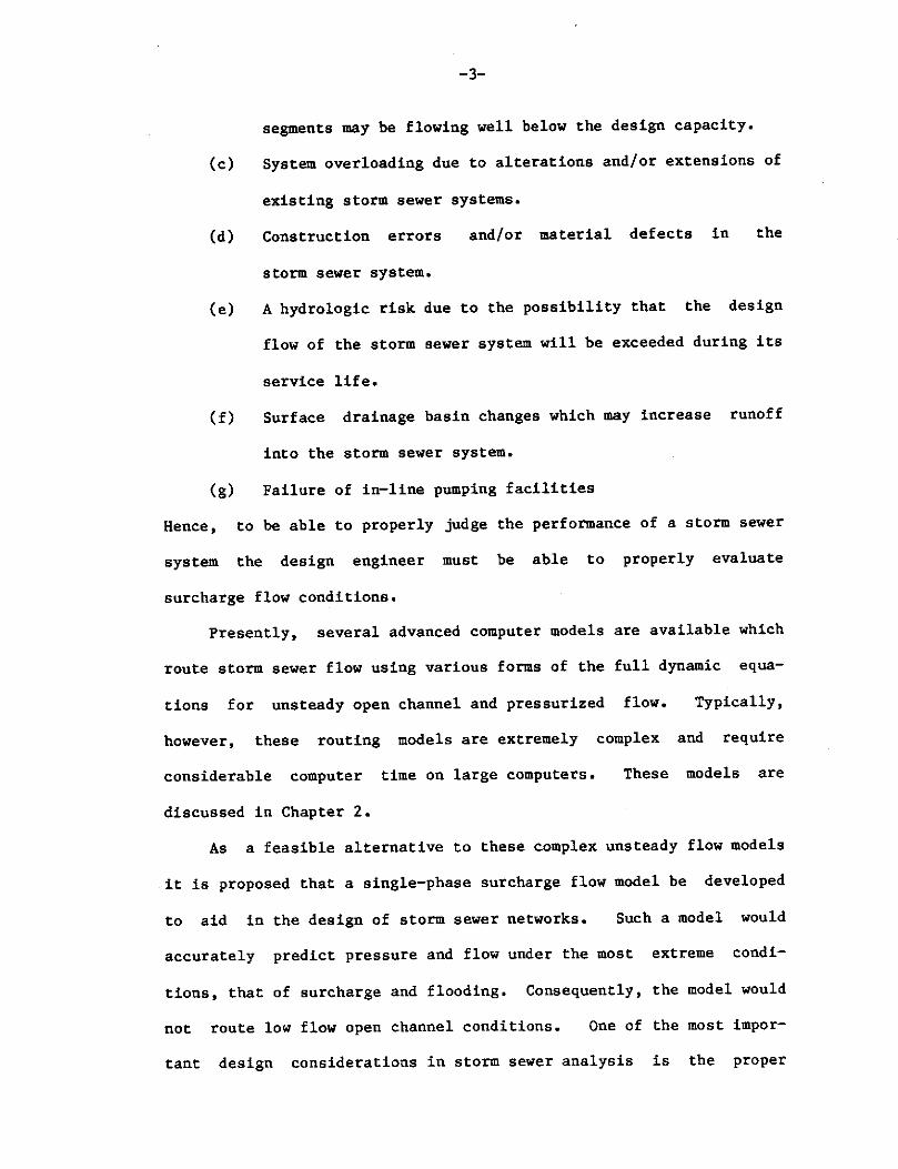
Several storm sewer flow models handle surcharge by using the
so-called Preissmann slot technique. These include the French model
CAREDAS (7); the Danish Hydraulic Institute model, System 11 Sewer
(15); and DAGVL-A and DAGVL-DIFF (28) developed at Chalmers
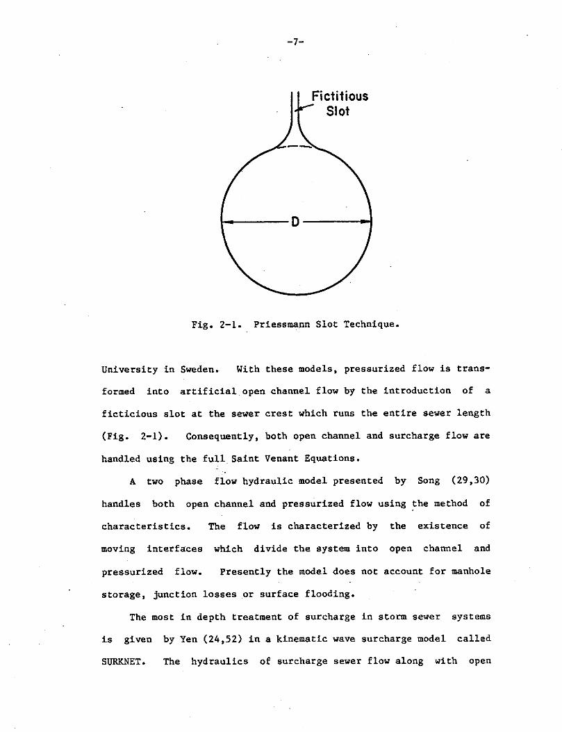
-7-
Fictitious Slot
Fig. 2-1. Priessmann Slot Technique.
University in Sweden. With these models, pressurized flow is trans-
formed into artificial open channel flow by the introduction of a
ficticious slot at the sewer crest which runs the entire sewer length
(Fig. 2-1). Consequently, both open channel and surcharge flow are
handled using the full Saint Venant Equations.
A two phase flow hydraulic model presented by Song (29,30)
handles both open channel and pressurized flow using the method of
characteristics. The flow is characterized by the existence of
moving interfaces which divide the system into open channel and
pressurized flow. Presently the model does not account for manhole
storage, junction losses or surface flooding.
The most in depth treatment of surcharge in storm sewer systems
is given by Yen (24,52) in a kinematic wave surcharge model called
SURKNET. The hydraulics of surcharge sewer flow along with open
-8-
channel flow are developed using the kinematic wave equations togeth-
er with Manning's formula to estimate the friction slope. Manhole
storage and surface flooding are accounted for through use of the
unsteady junction continuity equation. The present SURKNET model
solves for flow in the pipes independently in a cascading manner from
upstream towards downstream. A more advanced dynamic wave model
which solves the system of pipes simultaneously is being developed
and has not yet been published.
Wood (45,46) suggested that steady state pressurized flow theory
be applied to the analysis of surcharge in storm sewer systems. A
sewer network analysis is carried out by computing steady state
pressure and flow conditions at a specific point in time. These
steady flow conditions coupled with hydrograph inflows are used to
predict the change in manhole surface water levels over the next time
interval. The steady state solution is then obtained using the new
manhole water levels. The time step used for the simulation must be
small for accurate flow and pressure predictions.
Several other related surcharge flow models have been presented
by Bettess et al. (3), Martin and King (21) and Toyokuni (39).
2.3 Other Related Surcharge Work
Very little experimental data is available for storm sewer
systems operating under surcharge conditions. Land and Jobson (19)
developed an unsteady flow model for a single pipe subject to sur
charge conditions. The flow model was used with experimental pres
sure (water level) data to predict the discharge for a fully submerg
ed section of storm sewer. It is suggested that accurate simulta-
-9-
neous water level data is required for reasonable model predictions.
Nearly all the published surcharge prediction models utilize a
quasi-steady flow storage equation at the manhole junctions. Pre-
senty this is an acceptable method for analyzing the hydraulics of
storm sewer junctions. An unsteady pressurized junction continuity
relation has yet to be developed. Joliffe (18) has developed a
momentum balance steady flow continuity relation for open channel
sewer flow and applied it to unsteady flow behavior ay pipe junc
tions.
The energy and friction losses in storm sewer analysis are
handled using steady flow relations. Unsteady energy loss expres-
sions are nonexistant. Sangster et al. (27) performed experimental
studies on pressure losses at surcharged sewer junctions. Yevjevich
and Barnes (53) have studied both experimental and theoretical appli
cations of open channel flood routing through storm drains. Particu
lar attention is given to developing expressions for unsteady junc
tion box energy losses and these expressions need only be applied to
surcharge flow analysis.
THEORY OF ONE DIMENSIONAL UNSTEADY FLOW
Two basic mechanics equations are applied to a free body of
fluid to obtain two partial differential equations which describe
unsteady (transient) flow in closed conduits. These include: con
servation of mass (continuity) and Newton's second law of motion
(momentum). In this derivation the dependent variables are center
line pressure P(x,t) and the average velocity V(x,t) at a cross
section. The independent variables are position, x, measured along
the axis of the pipe and time, t. For convenience the pressure, P,
and velocity, V, are converted to the piezometric head, H, and flow
rate, Q, respectively. These continuity and momentum equations are
derived using the simplified free body approach similar to that used
by Wylie and Streeter (48), Thorley et al. (38), and Bergeron (2).
3.1 Equation of Continuity (Mass Conservation)
The continuity equation is developed from the law of conserva
tion of mass which states that the mass within a system remains
constant with time. Therefore,
dm/dt = 0 (3-1)
where mis the total mass of the system.
-10-
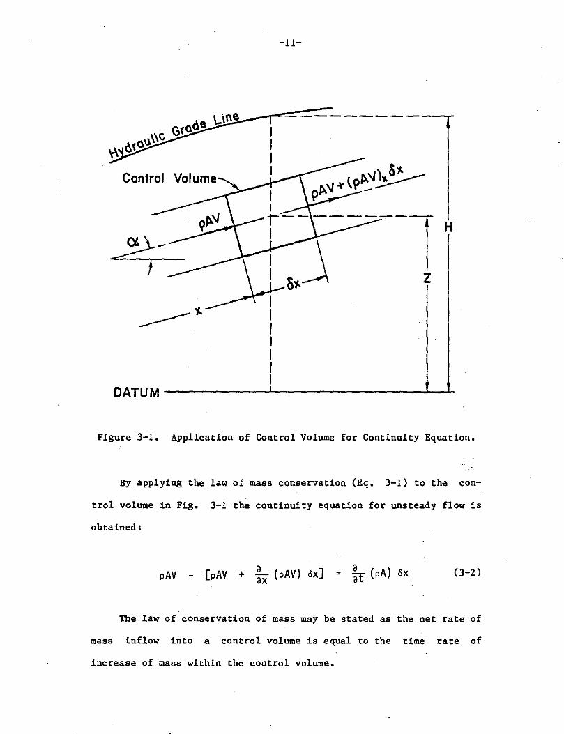
-11-
Control
H
z
Figure 3-1. Application of Control Volume for Continuity Equation.
By applying the law of mass conservation (Eq. 3-1) to the con
trol volume in Fig. 3-1 the co.ntinuity equation for unsteady flow is
obtained:
pAV [pAV + :x (pAV) ox] = ;t (pA) ox (3'-2)
The law of conservation of mass may be stated as the net rate of
mass inflow into a control volume is equal to the time rate of
increase of mass within the control volume.
-12-
Expanding Eq. 3-2 and rearranging yields
V aA Aax
1 aA + A at + y 2£.
p ax 1 ap av
+ ; at + ax = O (3-3)
The first four terms are the total derivatives of area A, and
density p, respectively. Therefore
where d = dt ( v
1 dA A dt
a ax
1 dp + p dt +
a + at)
il = 0 ax (3-4)
The first term of Eq. 3-4 describes the elasticity of the pipe
material and its rate of deformation with varying pressures. The
second term describes the compressibility of the liquid. The last
term accounts for the change in flow velocity at any instant. Equa-
tion 3-4 is valid for converging or diverging pipes, liquid or gas
flow since no simplifying assumptions have been made. However, this
work deals with prismatic conduits and utilizes the appropriate
assumptions. The reader is referred to Fluid Transients (48) for
proper handling of non-prismatic conduits.
To simplify the circumferential pipe expansion term
For prismatic conduits
1 dA A dt
1 dA A dt =
= .!. ( v aA + aA ) A ax at
aA ax
1 ,rrZ
m O and
a(1rr2 ) at = 2 ar
rat (3-5)
with
where r
strain.
By
-13-
ar = r ae:2 at at
is the pipe radius and e: 2 is the circumferential
combining Eqs. 3-5 and 3-6 and utilizing
1 dA A dt = 2ae:2 dP
~ dt
ae:2 at""" =
assuming that e:2
• f(P)
(3-6)
or hoop
ae:2 dP ~ dt
(3-7)
From the definition of bulk modulus of elasticity of fluid (32)
which gives
K =
1 dp pdt
dP (dp/p)
= 1 dP Kdf (3-8)
Substituting Eqs. 3-7 and 3-8 into Eq. 3-4 results in the
following form of the equation of continuity.
[2 k2 + .!_ ] dP + av aP K dt Pax = 0 . (3-9)
In order to further expand the term ae:2/aP it is necessary to
consider the manner in which the conduit deforms and various con-
straint conditions.
-14-
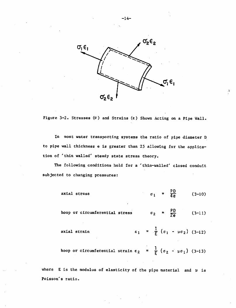
Figure 3-2. Stresses (a) and Strains(£) Shown Acting on a Pipe Wall.
In most water transporting systems the ratio of pipe diameter D
to pipe wall thickness e is greater than 25 allowing for the applica-
tion of 'thin walled' steady state stress theory.
The following conditions hold for a 'thin-walled' closed conduit
subjected to changing pressures:
axial stress a1 = PD (3-10) 4e
hoop or circumferential stress a2 = PD (3-11) 2e
1 axial strain £1 = E (a1 - µa2) (3-12)
hoop or circumferential strain e 2 = 1 E (a2 - µai} (3-13)
where E is the modulus of elasticity of the pipe material and µ is
Poisson's ratio.

-15-
~ 6 (a)
~ ~ (b)
' = 6 (c)
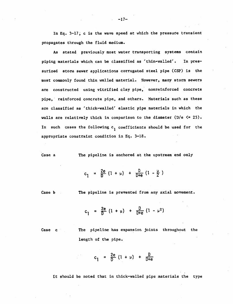
Figure 3-3. Pipeline Constraint Conditions.
Three possible constraint conditions exist as shown in Fig. 3-3:
Case a
Case b
The pipeline is anchored at the upstream end only.
From Eqs. 3-10, 3-11, 3-13 = 2~~ (1 - zl
therefore
= _Q_ (1 - H.) 2eE 2 (3-14)
The pipeline is prevented from any axial movement
From Eq. 3-12
From Eq. 3-13 = PD (1 - µ2) 2eE

-16-
therefore
(3-15)
Case c The pipeline has expansion joints throughout the
length of the pipe ( a1
• 0),
From Eq, 3-13
therefore
(3-16)
Equation 3-9 through substitution of l/c2 for the coefficient of
dP/dt takes the general form
il + 1 dP O P ax c2 dt =
in which
K/p c2 = ---"""-"-----1 + [ (KIE) (D/e)c1]
From Eqs, 3-14, 3-15 and 3-16, c1is defined _for each case:
{a)
(b)
(c)
c -1 1
cl• 1
cl = 1
- µ/2
2 - JJ
(3-17)
(3-18)
(3-19)
-17-
In Eq. 3-17; c is the wave speed at which the pressure transient
propagates through the fluid medium.
As stated previously most water transporting systems contain
piping materials which can be classified as 'thin-walled'. In pres-
surized storm sewer applications corrugated steel pipe (CSP) is the
most commonly found thin walled material. However, many storm sewers
are constructed using vitrified clay pipe, nonreinforced concrete
pipe,· reinforced concrete pipe, and others. Materials such as these
are classified as 'thick-walled' elastic pipe materials in which the
walls are relatively thick in comparison to the diameter (D/e <= 25).
In such cases the following c 1 coefficients should be used for the
appropriate constraint condition in Eq. 3-18.
Case a
Case b
Case c
The pipeline is anchored at the upstream end only
2e ) D ( µ) = D (l + µ + D+e l - 2
The pipeline is prevented from any axial movement.
= ~ (1 + µ) + _Q_ (1 - µ2) D+e
The pipeline has expansion joints throughout the
length of the pipe.
= ~e (1 + µ) + D
D+e
It should be noted that in thick-walled pipe materials the type
.,-18-
of constraint condition has little effect on the wave speed.
For composite materials such as reinforced concrete pipe, the
dimensionless coefficient, c1
, may be estimated by replacing the
actual pipe with an equivalent steel pipe based on the amount of
steel reinforcing and the thickness of the pipe. An equivalent steel
pipe thickness is obtained from the ratio of elastic modulus of
concrete to that of steel multiplied by the concrete thickness.
Other special considerations for materials such as plastic
pipes, lined concrete pipes, circular tunnels, etc. can be found in
Fluid Transients (48) from which the thick walled information was
obtained.
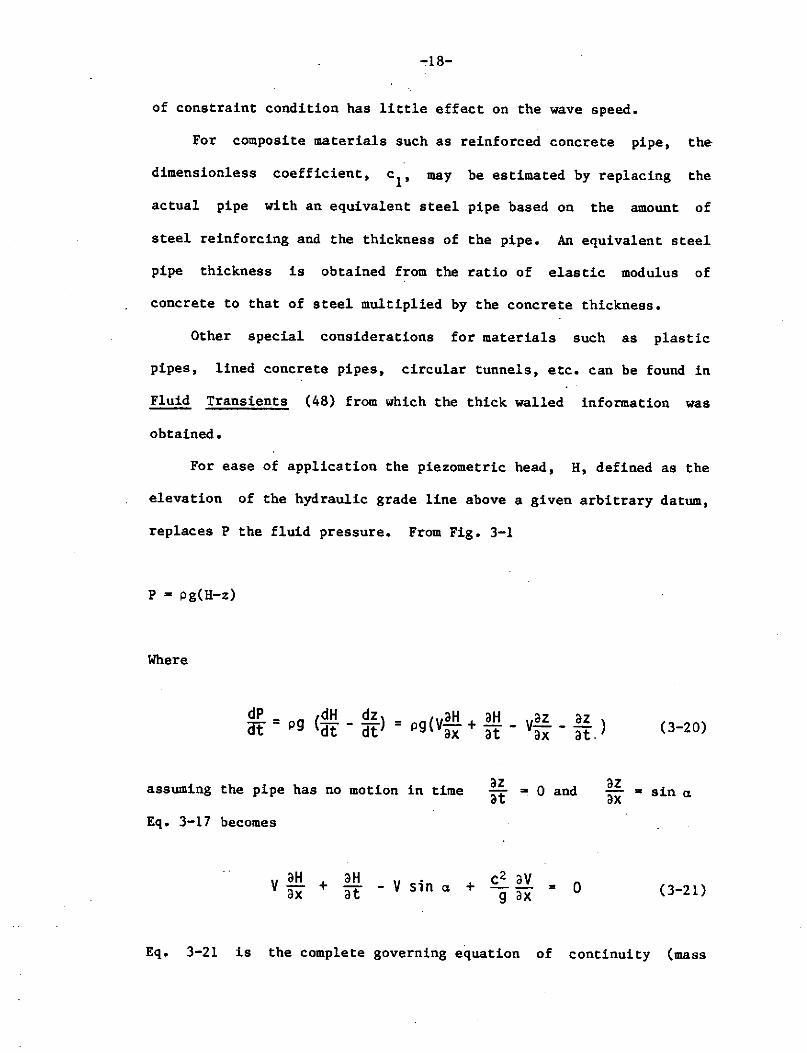
For ease of application the piezometric head, H, defined as the
elevation of the hydraulic grade line above a given arbitrary datum,
replaces P the fluid pressure. From Fig. 3-1
P • pg(H-z)
Where
dP dH dz cit'= pg (dt - dt) = g(v.fil!. + aH _ Vaz _ E_ )
P ax at ax at.
assuming the pipe has no motion in time
Eq. 3-17 becomes
V .fill. a H • ax + at - V s1n a
az ar•Oand
c2 av + -- = g ax 0
az ax
(3-20)
• sin a
(3-21)
Eq. 3-21 is the complete governing equation of continuity (mass
-19-
conservation) for one dimensional unsteady (transient) liquid flow in
prismatic conduits.
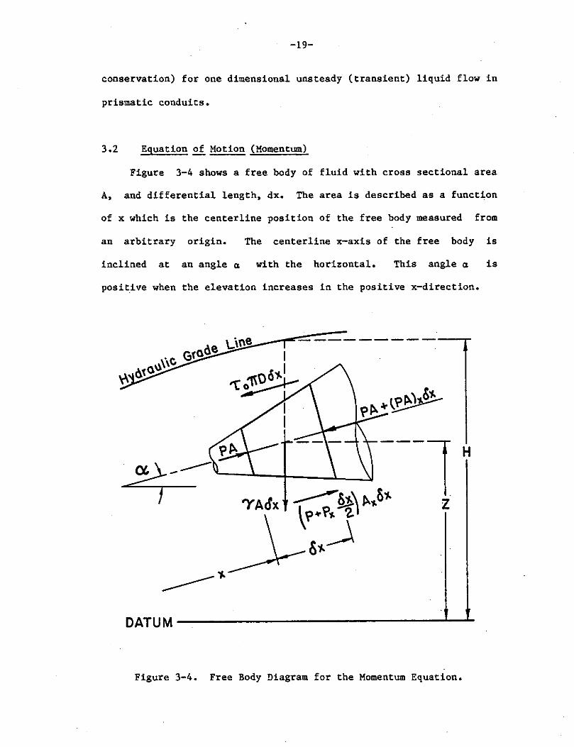
3.2 Equation of Motion (Momentum)
Figure 3-4 shows a free body of fluid with cross sectional area
A, and differential length, dx. The area is described as a function
of x which is the centerline position of the free body measured from
an arbitrary origin. The centerline x-axis of the free body is
inclined at an angle B with the horizontal. This angle B is
positive when the elevation increases in the positive x-direction.
-----------~
'YA&x
____ ..,. DATUM ______________ ..._..._
Figure 3-4. Free Body Diagram for the Momentum Equation.
-20-
Newton's second law of motion for a fluid element is defined as
i::F = d(mv) dt (3-22)
where mis the constant mass of the element and vis the velocity of
the mass center. l:F refers to the resultant of all external forces
acting on the element including body forces.·
Application of Newton's second law of motion to the free body
shown in Fig. 3-4 yields the following equation:
PA [PA + a(PA) ox] ax + [P + :: ~] !! ox
yA o x sin a = pA ox [V :~ + :~]
The left-hand side of the equation represents the forces acting
on the free body in the x-direction. They include the surface con-
tact normal pressures, the peripheral pressure components, the fric-
tional shear component, and the body force or gravity component,
Since the shear force, To, is considered a resistance to flow term it
is assumed to act in the - x direction. The right hand side of the
equation is simply the mass acceleration of the fluid body,
Neglecting the small quantity (ox) 2 and simplifying gives:·
A~ ax + T0~ D + yA sin a + av PAV ax +
av PA at = .0 (3-23)
It is necessary to make some assumptions concerning the
frictional shear resistance term, T0~n. If it is reasonable to

-21-
neglect frictional effects, the second term in Eq. 3-23 is zero.
Throughout this report, however, the frictional shear resistance term
is considered to be significant and is treated as if the flow is
steady. In terms of the Darcy-Weisbach friction factor, f (32):
(3-24)
This equation is developed from the Darcy-Weisbach equation of the
form
= pfLV I VI 20 (3-25)
and a force balance (Fig. 3-5) on a pipe under steady state flow
conditions
(3-26)
The absolute value sign is applied to the velocity term in Eq. 3-24
to insure that the shear stress always opposes the direction of flow.
'Lo'TfDD.L
2 t ~pD,r D 4 _J_
l-----~L-l
Figure 3-5. Force Balance on a Pipe.
-22-
Until recently the shear stress or friction term in an unsteady
flow analysis was often neglected or the friction factor, f, was
assumed constant for a given simulation. This was due primarily to
the mathematical difficulty of modeling the friction term for a wide
range of continuously changing flowrates. Traditional methods of
determining f were based on the Moody diagram (23), a graphical
procedure or empirical implicit formulas such as those developed by
Colebrook (10). In 1966 Wood (43) developed the first empirical
explicit friction factor relationship of the Colebrook equation. And
most recently, in 1976, Swamee and Jain (33) developed the following
explicit formula for f with several restrictions placed on it.
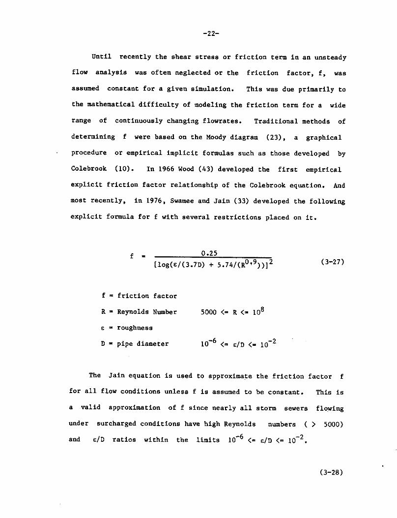
f = 0.25
[log(e/(3.7D) + 5.74/(R0,9))]2 (3-27)
f = friction factor
R = Reynolds Number 5000 <= R <= 108
e: a roughness
D = pipe diameter
The Jain equation is used to approxima.te the friction factor f
for all flow conditions unless f is assumed to be constant. This is
a valid approximation of f since nearly all storm sewers flo.wing
under surcharged conditions have high Reynolds numbers ( > 5000)
and e:/D ratios within the limits 10-6 <= e:/D <= 10-2•
(3-28)
-23-
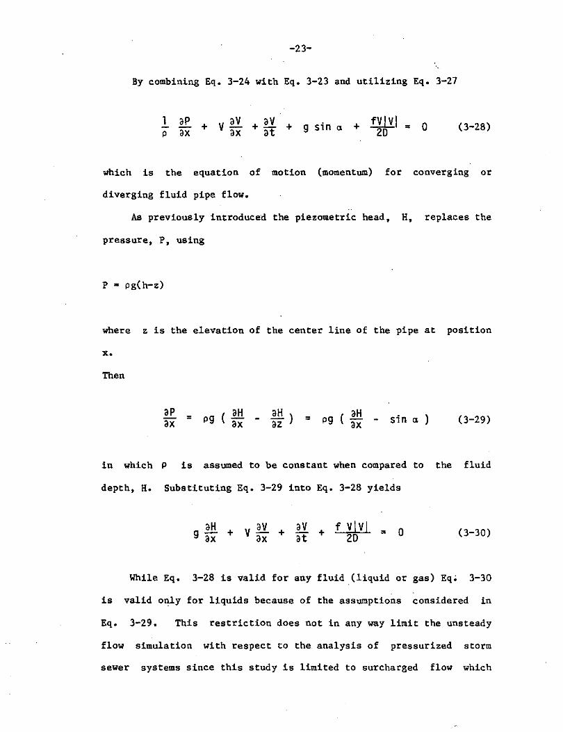
By combining Eq. 3-24 with Eq. 3-23 and utilizing Eq. 3-27
1 p
aP ax + g sin a + fV!VI =
20 0 (3-28)
which is the equation of motion (momentum) for converging or
diverging fluid pipe flow.
As previously introduced the piezometric head, H, replaces the
pressure, P, using
P • pg(h-z)
where z is the elevation of the center line of the pipe at position
x.
Then
aP ax = ( aH aH
pg ax - az ) = ( aH pg - -ax sin a) (3-29)
in which P is assumed to be constant when compared to the fluid
depth, H. Substituting Eq. 3-29 into Eq. 3-28 yields
+ v ~ + av + ax at
f VIVI 20 = 0 (3-30)
While Eq. 3-28 is valid for any fluid (liquid or gas) Eq; 3-30
is valid only for liquids because of the assumptions considered in
Eq. 3-29. This restriction does not in any way limit the unsteady
flow simulation with respect to the analysis of pressurized storm
sewer systems since this study is limited to surcharged flow which

-24-
neglects any formation of air pockets or cavities within the system.
Therefore Eq. 3-30 is the governing equation of motion (momentum) for
one dimensional unsteady (transient) liquid flow as applied to pres-
surized liquid systems.
3.3 Governing Equations for Unsteady Surcharged Sewer Flow
Summarizing the theoretical development, the.two governing dif-
ferential equations for one dimensional unsteady flow in slightly
deformable conduits are:
Continuity: v l!:! ax aH
+ af - V sin a
Momentum: g aH + ax v il + ax
av at +
c2 av + g ax =
fVIVI 20 =
0 (3-21)
0 (3-30)
These are quasi-linear hyperbolic partial differential equations
containing two dependent variables (P,V) and two independent
variables (x,t). The pressure and velocity of the liquid are a
function of both the position and the time from which the steady
state conditions are disturbed.
In general, a hydraulic analysis of a storm sewer system is
considered a slowly varying transient phenomena. Therefore, several
terms in Eqs. 3-21 and 3-30 can be justifiably neglected when appli-
cation is restricted to this type of slowly varying flow problem.
In both Eqs. 3-21 and 3-30 the convective acceleration terms
V( av/ax) and V(aH/3x) are always small when compared to the local
acceleration terms a V /at and a H/a t respectively. They are
-25-
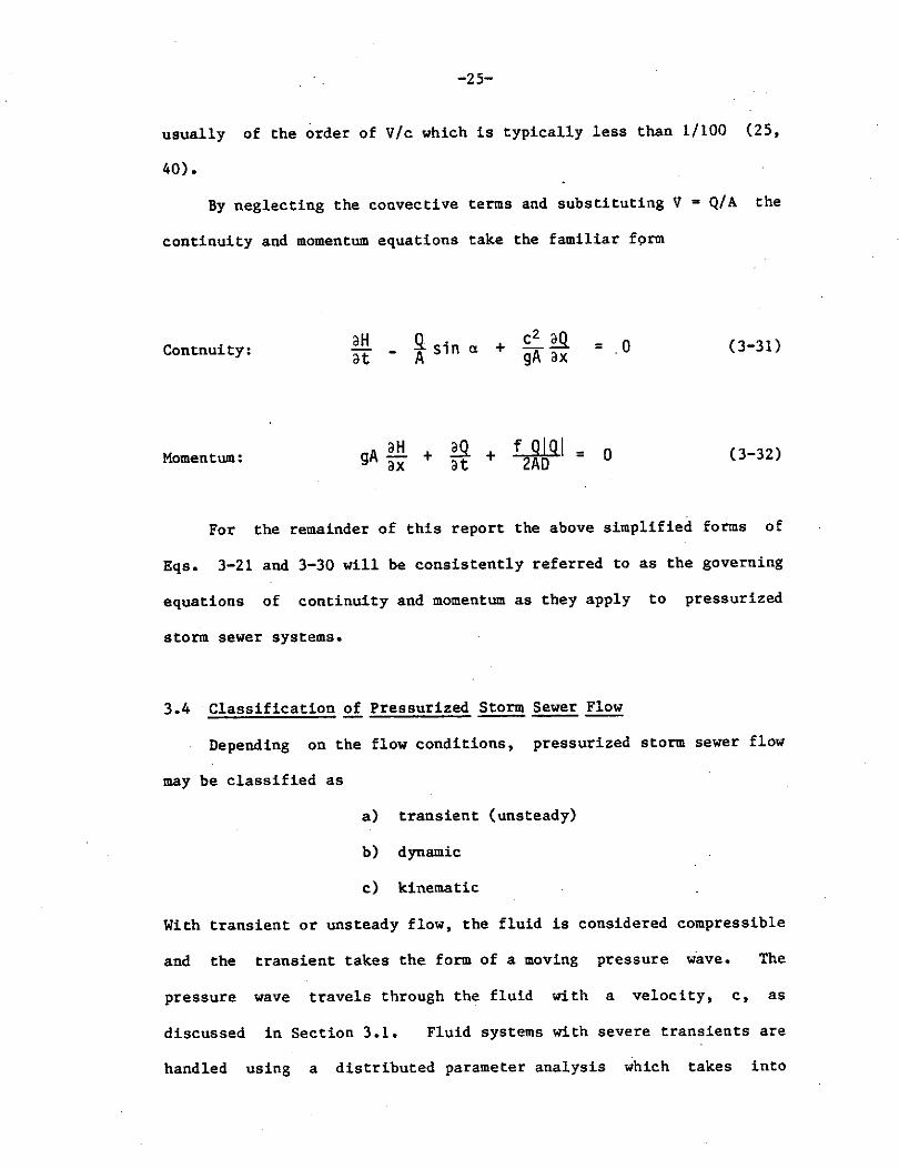
usually of the order of V/c which is typically less than 1/100 (25,
40).
By neglecting the convective terms and substituting V = Q/A the
continuity and momentum equations take the familiar form
Contnuity:
Momentum:
aH at i sin a + ~ 2..!l.
gA ax = _o
gA :~ + ~ + ;w.t = O
(3-31)
(3-32)
For the remainder of this report the above simplified forms of
Eqs. 3-21 and 3-30 will be consistently referred to as the governing
equations of continuity and momentum as they apply to pressurized
storm sewer systems.
3.4 Classification of Pressurized Storm Sewer Flow
Depending on the flow conditions, pressurized storm sewer flow
may be classified as
a) transient (unsteady)
b) dynamic
c) kinematic
With transient or unsteady flow, the fluid is considered compressible
and the transient takes the form of a moving pressure wave. The
pressure wave travels through the fluid with a velocity, c, as
discussed in Section 3.1. Fluid systems with severe transients are
handled using a distributed parameter analysis which takes into
-26-
account the fluid and pipe elasticity (capacitance), the fluid
inertia and the frictional losses. The distributed parameter model
is discussed in Section 4.1.
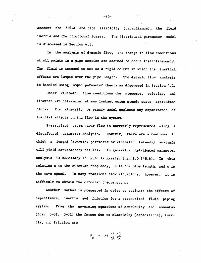
In the analysis of dynamic flow, the change in flow conditions
at all points in a pipe section are assumed to occur instantaneously.
The fluid is assumed to act as a rigid column in which the inertial
effects are lumped over the pipe length. The dynamic flow analysis
is handled using lumped parameter theory as discussed in Section 4.2.
Under kinematic flow conditions the pressure, velocity, and
flowrate are determined at any instant using steady state approxima-
tions. The kinematic or steady model neglects any capacitance or
inertial effects on the flow in the system.
Pressurized storm sewer flow is correctly represented using a
distributed parameter analysis. However, there are situations in
which a lumped (dynamic) parameter or kinematic (steady) analysis
will yield satisfactory results. In general a distributed parameter
analysis is necessary if wL/c is greater than 1.0 (48,6). In this
relation w is the circular frequency, Lis the pipe length, and c is
the wave speed. In many transient flow situations, however, it is
difficult to obtain the circular frequency, w.
Another method is presented in order to evaluate the effects of
capacitance, inertia and friction for a pressurized fluid piping
system. From the governing equations of continuity and momentum
(Eqs. 3-31, 3-32) the forces due to elasticity (capacitance), iner-
tia, and friction are
= at c2 ~ gA ax
-27-
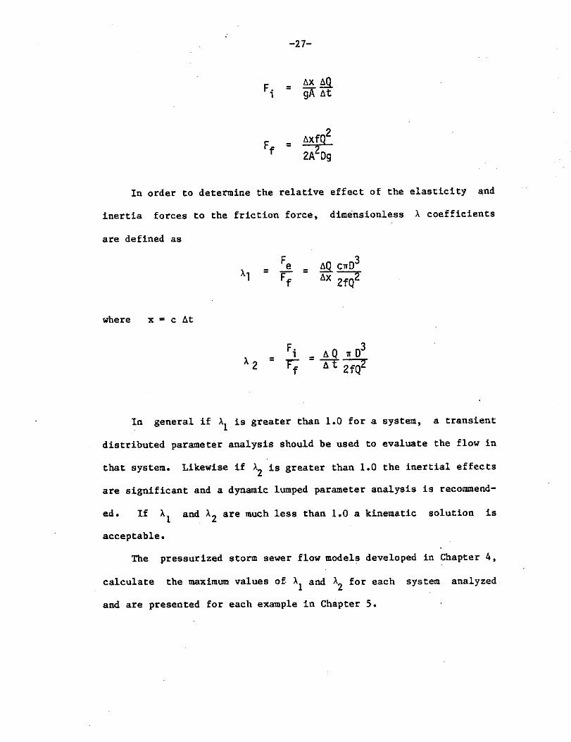
=
= llx~Q2
2A Dg
In order to determine the relative effect of the elasticity and
inertia forces to the friction force, dimensionless A coefficients
are defined as
=
where x = c llt
=
In general if Al is greater than 1.0 for a system, a transient
distributed parameter analysis should be used to evaluate the flow in
that system. Likewise if >-i is greater than 1.0 the inertial effects
are significant and a dynamic lumped parameter analysis is recommend-
ed. If Al and Az are much less than 1.0 a kinematic solution is
acceptable.
The pressurized storm sewer flow models developed in Chapter 4,
calculate the maximum values of Al and A2
for each system analyzed
and are presented for each example in Chapter 5.

PRESSURIZED STORM SEWER SYSTEM MODELS
Three numerical hydraulic flow models are developed for the
analysis of storm sewer systems at peak flows. These include a
finite element unsteady distributed parameter model, a dynamic lumped
parameter model and a kinematic (steady state with storage) model.
In this chapter, each model is formulated and presented with the
appropriate assumptions. In addition, Sections 4.4 and 4.5 describe
the boundary conditions which are incorporated into the system equa-
tions for each flow model. For each numerical method, a computer
flow model program is written and presented in Chapter 7.
4.1 Finite Element Model
In this section a numerical solution of the complete governing
flow equations of momentum and continuity for pressurized storm sewer
systems is presented using the finite element method (FEM). The
finite element method described here is the basis for an unsteady
distributed parameter flow model. The solution is obtained by solv
ing Eqs. 3.31 and 3.32 simultaneously with appropriate simplifying
assumptions and boundary conditions.
follows.
A brief description of the FEM
The FEM is a numerical procedure for solving differential equa-
tions of physics and engineering. The fundamental concept of the FEM
is that any continuous quantity such as temperature, pressure, flow
or displacements can be approximated by a discrete model composed of
~2s-

-29-
a set of piecewise continuous functions defined over a finite number
of subdomains.
The discrete model is constructed as follows:
(a) A finite number of points in the domain is identified.
These points are called nodes.
(b) The value of the continuous quantity is denoted as a
variable which is to be determined.
(c) The domain is divided into a finite number of subdomains
called elements. These elements are connected at common
nodal points and collectively approximate the shape of the
domain.
(d) The continuous quantity is approximated over each element
by a polynomial that is defined using the nodal values of
the continuous quantity. A different polynomial is
defined for each element but the element polynomials can
be selected in such a way that continuity is maintained
along the element boundaries.
For the FEM application to unsteady flow in storm sewer systems
the governing momentum and continuity equations are solved using the
Galerkin method of weighted residuals. The procedure is presented in
texts by Zienkiewicz (54) and Huebner (16). In general, the Galerkin
finite element technique involves:
(a) identification of the approximating polynomials Q = Q(x),
H = H(x), etc. which contain the unknowns to be determined
(b) multiplication of Eqs. 3,31 and 3.32 by weighting functions
derived from the approximating functions Q(x), H(x), etc.
(c) substitution of the approximating polynomials Q(x), H(x),
-30-
etc. into Eqs. 3.31 and 3.32.
(d) integration of these modified equations over the element to
form a set of ordinary differential equations in time, and
(e) integration of the ordinary differential equations over
time.
The Galerkin finite element method described herein is based on
representing the unknown variables, Q and H·on a local element basis.
The entire global solution domain is discussed following this formu-
lation.
One of the distinct advantages of using the finite element
method is the ability to choose the approximati_ng polynomials for the
dependent variables. Several possibilities exist. However, there is
a direct relationship between the computational efficiency and the
order of the approximating polynomials.
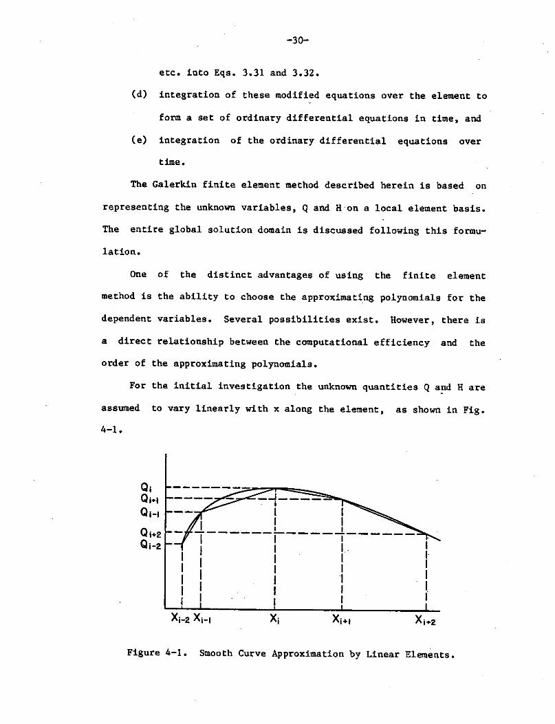
For the initial investigation the unknown quantities Q a~ Hare
assumed to vary linearly with x along the element, as shown in Fig.
4-1.
Q1 Q1·1
Q1-1
Q1+2 Q;-2
-~--..J ____ _ I I
I ! I I - -I -- I -----
I I 1 .. I I I I I I I I I
I l : X; X1+1
Figure 4-1. Smooth Curve Approximation by Linear Elements.
-31-
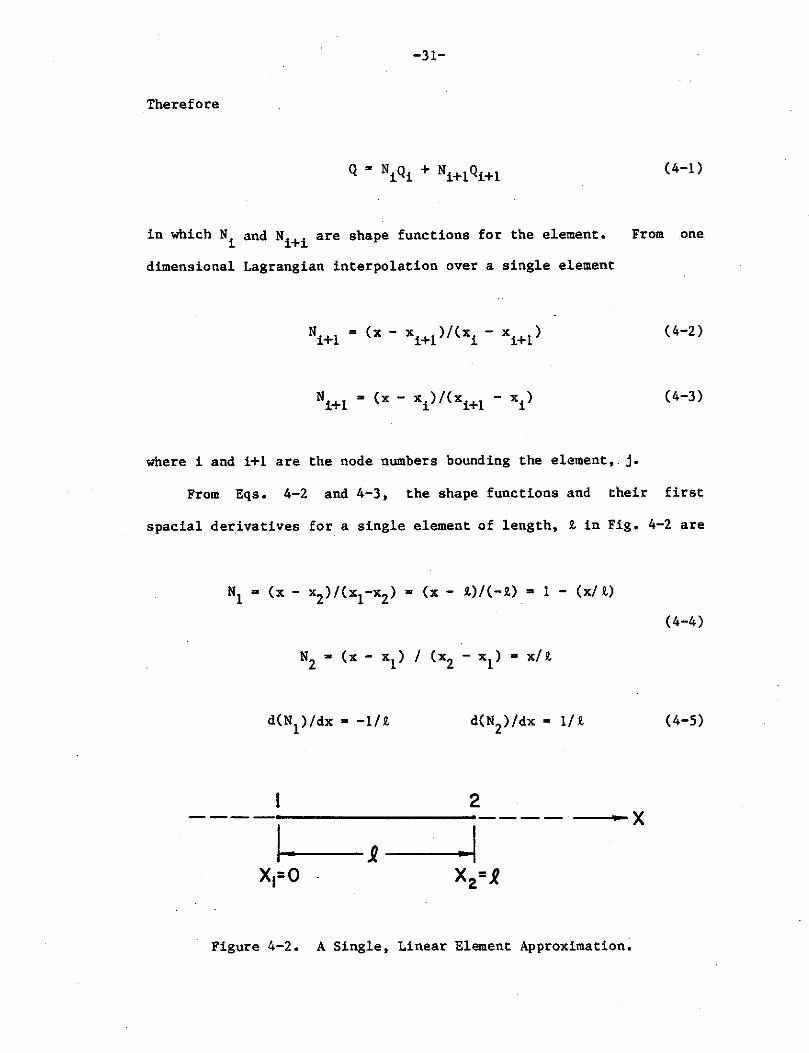
Therefore
in which Ni and Ni+i are shape functions for the element.
dimensional Lagrangian interpolation over a single element
(4-1)
From one
(4-2)
(4-3)
where i and i+l are the node numbers bounding the element,. j.
From Eqs. 4-2 and 4-3, the shape functions and their first
spacial derivatives for a single element of length, i in Fig. 4-2 are
(4-4)
(4-5)
2 ----- --- x I . .1
x,=o X2=.e
Figure 4-2. A Single, Linear Element Approximation.
-32-
Substitution of Eq. 4-4 into Eq. 4-1 and expressing in matrix form
yields
Q = LNJ {Q} (4-6)
A similar derivation is performed on the variable, H. Quanti-
ties such as g, A, D and care considered·constant over the element
length.
The Galerkin method, in general, requires that
f {N}.,e (6)dn = {0} n
where ..e is the differential operator acting on the unknown field
variable (Q,H) over the system domain SI, and N are the approximating
polynomials or shape functions.
Applying the Galerkin method to the governing differential
equations (Eqs. 3-31 and 3-32) yields
and
i: e
l: e
! 1 {N}( aH - QA sin a + o at
c2 2.!!. gA ax) dx
ft {N}( 2.!!. + gA .ill + fA 00101 ) dx O at ax ~
= {O} (4-7)
= {O} (4-8)
Through appropriate substitution of the element shape functions (Eq.
4-6)
-33-
. i: ! i {N}[ LNJ{H} - si~ 0 LNJ{Q} + 0 e
2 . ~A d~~J {Q} ] dx = {O}
i: 11 {N}[ LNJ{Q} + gA ddLNJ {H} + e o x
2k0 LNJfflLNJflQI }lNJ{Q} ] dx = {O}
(4-9)
(4-10)
where the dot over the dependent variable represents differentiation
with respect to time.
where
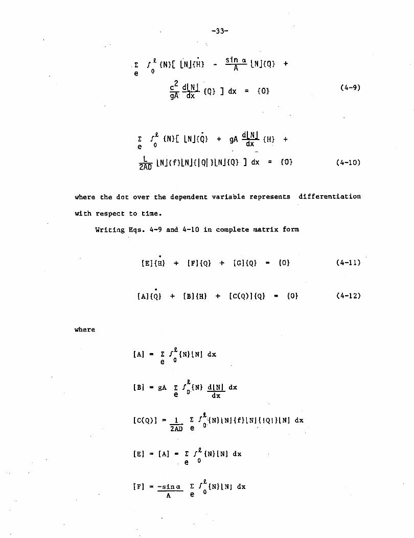
Writing Eqs. 4-9 and 4-10 in complete matrix form
• [El {H} + [Fl {Q} + [Gl {Q} a {O}
• [Al{Q} + [Bl{H} + [C(Q) ){Q} a {O}
R, [Bl a gA l: ! {N} dlNJ dx
e o· ~
R, [C(Q)] • l l: f O {N}lNJ{f}lNJ{ IQI }lNJ dx
ZAD e
[El a [Al = l: ft {N}lNJ dx e o
[Fl a -sina A
(4-11)
(4-12)

-34-
[G] = c2 l: /· {N} d[N] dx gX e o """"cix
Here the nonlinear friction term, [C(Q)] is linearized by assum-
ing that the unknown variable, IQI , in the friction term is known
from the previous time step. This assumption is valid since the.
friction term does not vary substantially over the time interval.
Evaluation of [A], [B), [C(Q)), [El. [Fl, and [G] yields
[A) = L ~;: :;:]
[B) = gA r-1/2 1/~
l:112 1/~
[C(Q)) = L 2AD
rc(l,l) C(l,2~
~(2,1) C(2,2~
where
C(l,l) = (l/S)f11Q1 1 + (l/20)f2 1Q11 + (l/20)f1
1Q2
1 + (l/30)f2
1Q2
1
C(l,2) = (l/20)f11q11 + (l/30)f2 1Q11 + (l/30)f1
1q2
1 + (l/20)f2
1Q2
1
C(2,l) = (l/20)f1IQ1I + (l/30)f2IQ1I + (l/30)fl1Qzl + (l/20)fz1Qzl
C(2,2) = (l/30)f11q11 + (l/20)£2 1q1 1 + (l/20)f1
1Q2
1 + (l/S)f2
1Q2
1
[E] = L ~/] 1/~ 1/6 1/3
~,, ''J [F) = -L sin a A /6 1/3
[G] 2 r-1,2 1121
• ~A l-1/2 · l/~
-35-
This concludes the finite element formulation with respect to
the spacial domain. In order to evaluate the time dimension or
transient effect in the governing equations the Galerkin method is
again used.
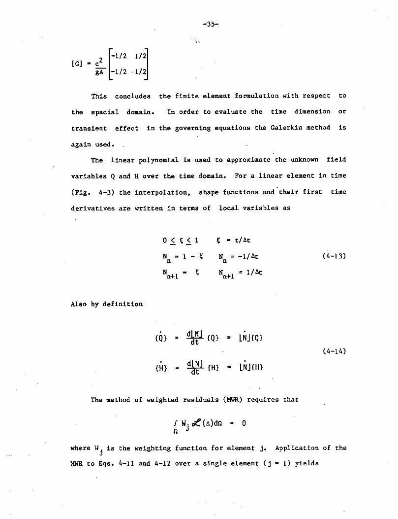
The linear polynomial is used to approximate the unknown field
variables Q and Hover the time domain. For a linear element in time
(Fig. 4-3) the interpolation, shape functions and their first time
derivatives are written in terms of local variables as
Also by definition
O i I; i l I; = ti lit
N =l-1; n
Nn+l • I;
{Q} = £IJ!.I. { Q } dt
N = -1/llt n
Nn+l = 1/llt
. = LNJ{Ql
{H} = dLNJ {H} dt
= .
LNJ{H}
The method of weighted residuals (MWR) requires that
f w. ol'(ti)dsi = 0 SJ J
(4-13)
(4-14)
where Yj is the weighting function for element j. Application of the
MWR to Eqs. 4-11 and 4-12 over a single element (j = l) yields
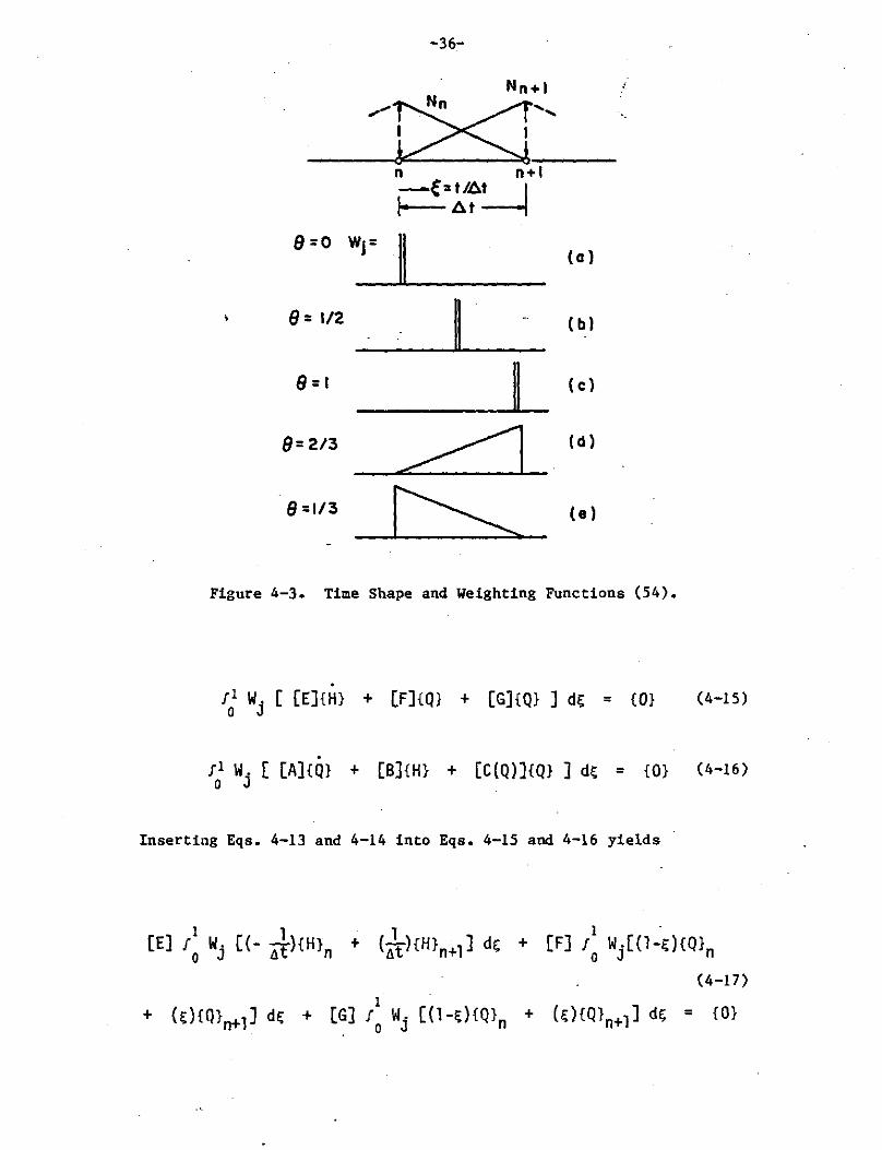
-36-
Nn+I
"t><f' n n+I -e=•t.6~ I .6t
8 =O Wj=
II (a)
8= 1/2 ~ (bl
8 = I ~ (cl
8= 2/3 ~ (d)
e =113 ~ (el
Figure 4-3. Time Shape and Weighting Functions (54) •
. 1; Wj [ [E]{H} + (F]{Q} + [G]{Q}] dt = {0} (4-15)
1; Wj [ [A]{Q} + [B]{H} + [C(Q)]{Q}] dt = {O} (4-16)
Inserting Eqs. 4-13 and 4-14 into Eqs. 4-15 and 4-16 yields
[E] < Wj [(-11
~){H}n + (11\){H}n+lJ df; + [F] 1: Wj[(l~f;){Q}n
(4-17)
-37-
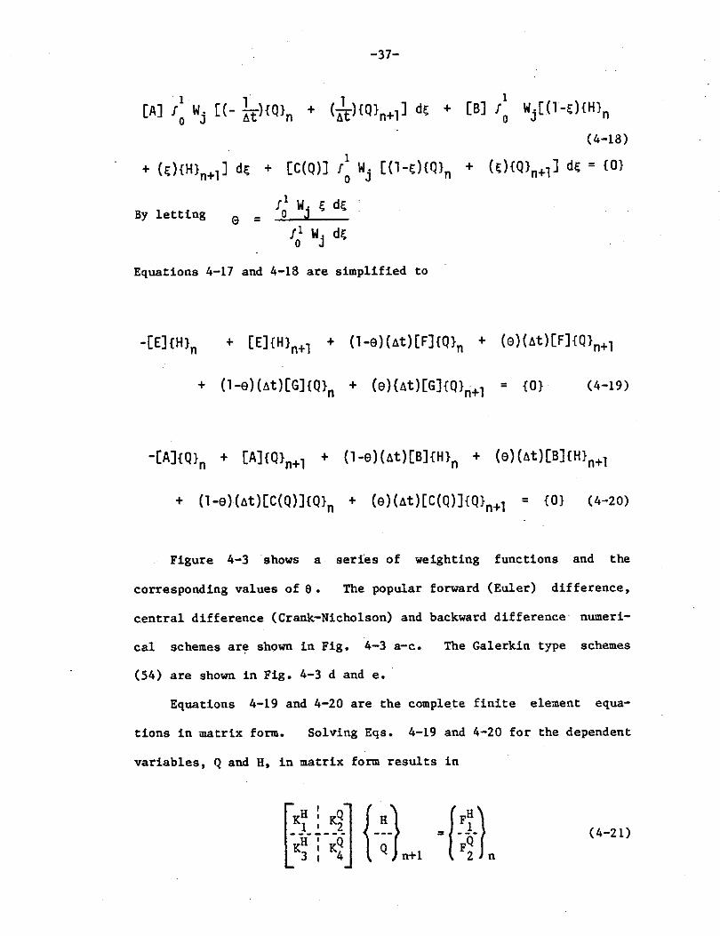
[A] < Wj [(- !t){Q}n + (it){Q}n+l] dE; + [BJ f: Wj[(l-e;){H}n
(4-18) 1
+ (e;){H}n+l] de; + [C(Q)] r0
Wj [(1-E;){Q}n + (E;){Q}n+l] de;= {O}
By letting a = f~ Wj E; dE; r01 wj dE;
Equations 4-17 and 4-18 are simplified to
-[E]{H}n + [E]{H}n+l + (1-e)(At)[F]{Q}n + (e)(At)[F]{Q}n+l
+ (1-e)(At)[G]{Q}n + (e)(At)[G]{Q}n+l = {O} (4-19)
-[A]{Q}n + [A]{Q}n+l + (1-e)(At)[B]{H}n + (e)(At)[B]{H}n+l
+ (1-e)(At)[C(Q)]{Q}n + (e)(At)[C(Q)]{Q}n+l = {O} (4-20)
Figure 4-3 shows a series of weighting functions and the
corresponding values of a. The popular forward (Euler) difference,
central difference (Crank-Nicholson) and backward difference· numeri-
cal schemes are shown in Fig. 4-3 a-c. The Galerkin type schemes
(54) are shown in Fig. 4-3 d and e.
Equations 4-19 and 4-20 are the complete finite element equa-
tions in matrix form. Solving Eqs. 4-19 and 4-20 for the dependent
variables, Q and H, in matrix form results in
(4-21)
-38-
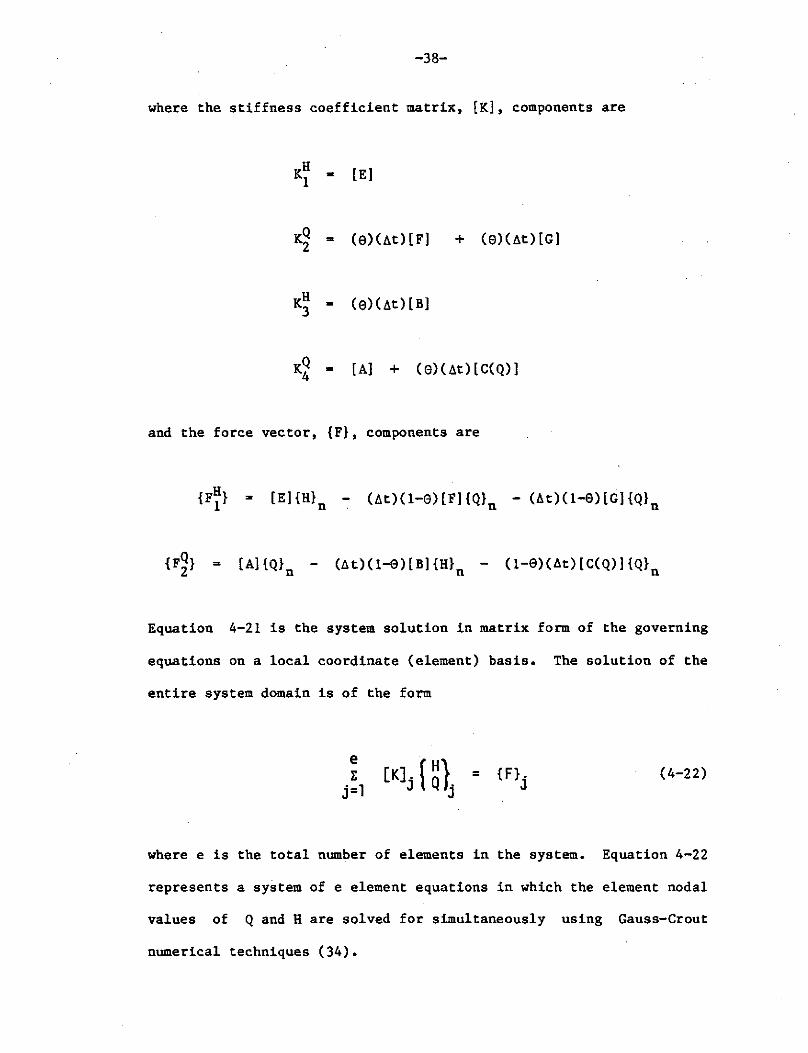
where the stiffness coefficient matrix, [K], components are
KH • [E] 1
KQ 2 = Ce><at> [Fl + Ce>Cat)[G]
KH • Ce>Cat) [BJ 3
KQ 4 = [A] + Ce)(at)[C(Q)l
and the force vector, {F}, components are
[E]{H}n ~ (at)(l-e)[F]{Q}n - (l1t)(l-6)[G){Q}n
= [A){Q}n - (l1t)(l-0)[B]{H}n - (l-0)(l1t)[C(Q)]{Q}n
Equation 4-21 is the system solution in matrix form of the governing
equations on a local coordinate (element) basis. The solution of the
entire system domain is of the form
e &
j=l = (4-22)
where e is the total number of elements in the system. Equation 4-22
represents a system of e element equations in which the element nodal
values of Q and Hare solved for simultaneously using Gauss-Crout
numerical techniques (34).
-39-
Throughout ·the system various initial and boundary conditions
are incorporated into the system equations. These conditions are
discussed in Section 4.4 and 4.5.
4.2 Dynamic Lumped Parameter Model
Since fluid piping systems are continious the complete governing
equations of unsteady flow are correctly soived using a distributed
parameter model, in which the elastic behavior of the fluid and pipe
material, the fluid inertia and the frictional resistance are dis-
tributed along the pipeline. The finite element model described in
Section 4.1 is a distributed parameter model. There is, however, a
large class of fluid transient problems in which it is permissible to
use a lumped parameter or rigid column theory analysis with certain
simplifying assumptions. These include slowly varying transient flow
situations such as that in surcharged storm sewer systems.
From Chapter 2. the governing equations for pressurized storm
sewer analysis are:
Continuity: aH l sin a + c2 2..\2.
0 at - gA ax = (3-31)
aH 2..\2. + f glgl = 0 gA ax + at 2AD Momentum: (3-32)
The dynamic-lumped parameter model developed in this thesis
makes three distinct assumptions concerning the capacitance, pipe
slope and inertia of the system:
Capacitance: In this model the elastic behavior of the fluid is
-40-
considered negligible as compared to friction and inertial effects.
Therefore Eq. 3-31 takes the form
dH Q. dt - A sin a = 0 (4-23)
Pipe Slope: Most storm sewer systems are designed as gravity flow
(open channel) systems in which the potential head to create flow in
the system is provided by a change in elevation or slope in the
direction of the flow path. Typical storm sewer systems have pipes
with longitudinal slopes which may vary from 0.000 ft./ft. to 0.010
ft./ft. However, in this model the effect of pipe slope on the
continuity equatio~ is considered negligible since sin a· a O for
small angles. Hence, Eq. 4-23 reduces to dH/dt = 0 which describes
steady state continuity conditions for a pipe element. A useful form
of the incompressible, steady flow continuity equations is
Q • AV (4-24)
where: Q is the discharge, A is the cross sectional flow area and V
is the average velocity over area A.
Lumped Inertia: As with the continuity equation, the momentum equa-
tion is simplified for incompressible flow by assuming the pipe
elements to be inelastic. Therefore, the liquid mass is treated as a
rigid column (Fig. 4-4) in which the inertial forces are lumped
together over the pipe length L. The modified lumped parameter
momentum equation is an ordinary differential equation of the form
-41-
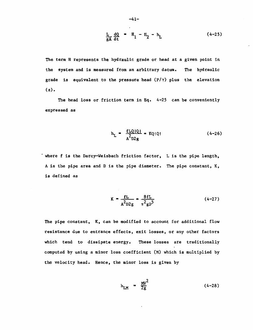
!:.__ ~ • H1 - 11i - ~ gA dt
(4-25)
The term H represents the hydraulic grade or head at a given point in
the system and is measured from an arbitrary datum. The hydraulic
grade is equivalent to the pressure head (P/y) plus the elevation
(z).
The head loss or friction term in Eq. 4-25 can be conveniently
expressed as
KQIQI (4-26)
- where f is the Darcy-Weisbach friction factor, Lis the pipe length,
A is the pipe area and Dis the pipe diameter. The pipe constant, K,
is defined as
K• = (4-27)
The pipe constant, K, can be modified to account for additional flow
resistance due to entrance effects, exit losses, or any other factors
which tend to dissipate energy. These losses are traditionally
computed by using a minor loss coefficient (M) which is multiplied by
the velocity head. Hence, the minor loss is given by
(4-28)
-42-
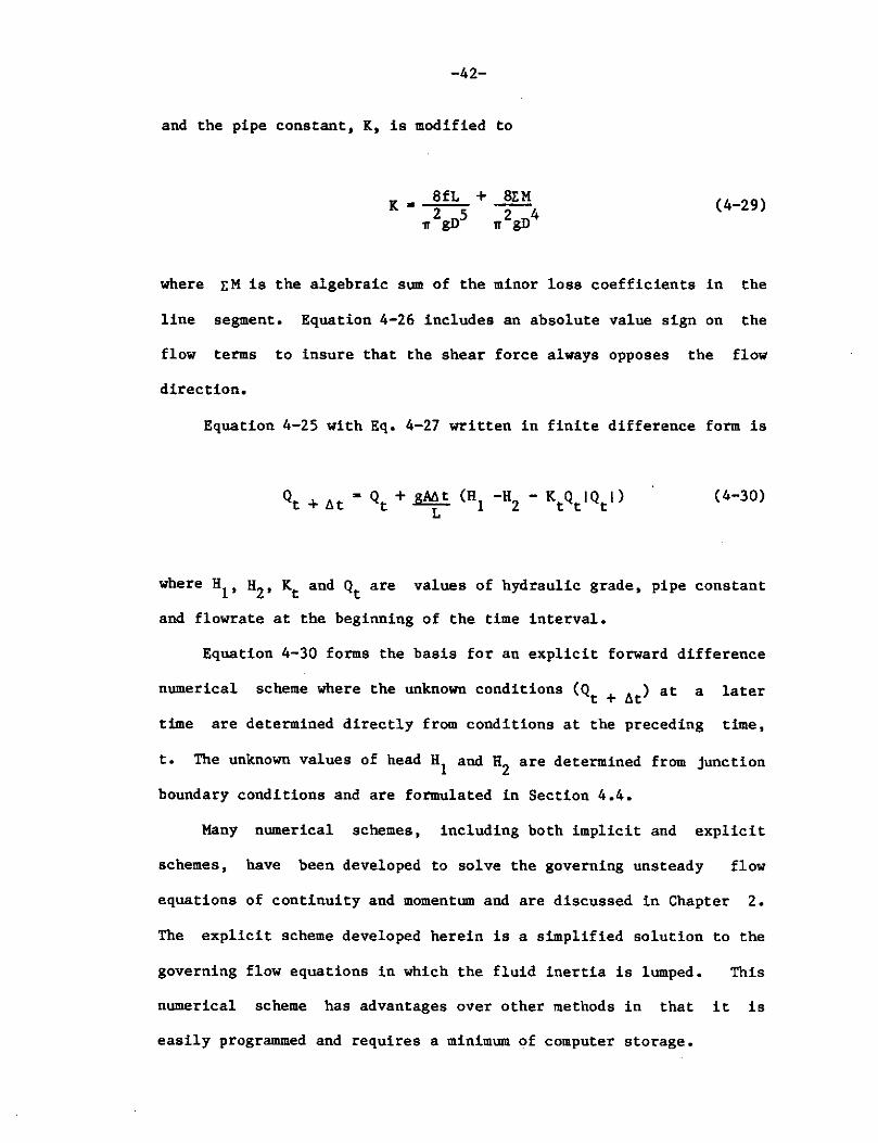
and the pipe constant, K, is modified to
K • 8fL 2 05
11 g
+ 82:M
,r2gD4 (4-29)
where i:M is the algebraic sum of the minor loss coefficients in the
line segment. Equation 4-26 includes an absolute value sign on the
flow terms to insure that the shear force always opposes the flow
direction.
Equation 4-25 with Eq. 4-27 written in finite difference form is
(4-30)
where H1, H2 , Kt and Qt are values of hydraulic grade, pipe constant
and flowrate at the beginning of the time interval.
Equation 4-30 forms the basis for an explicit forward difference
numerical scheme where the unknown conditions (Qt+ bt) at a later
time are determined directly from conditions at the preceding time,
t. The unknown values of head H1
and H2
are determined from junction
boundary conditions and are formulated in Section 4.4.
Many numerical schemes, including both implicit and explicit
schemes, have been developed to solve the governing unsteady flow
equations of continuity and momentum and are discussed in Chapter 2.
The explicit scheme developed herein is a simplified solution to the
governing flow equations in which the fluid inertia is lumped. This
numerical scheme has advantages over other methods in that it is
easily programmed and requires a minimum of computer storage.
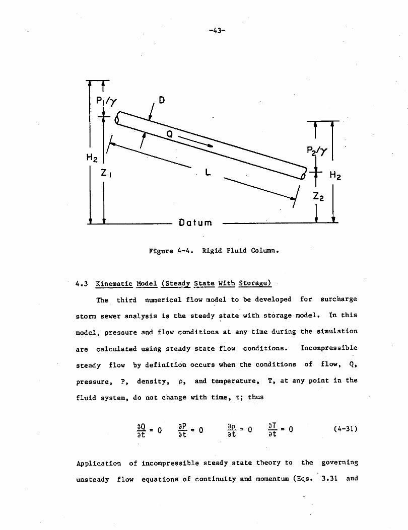
-43-
H2 ~ t H2 z, L
Z2 I Datum l Figure 4-4. Rigid Fluid Column.
4.3 Kinematic Model (Steady State With Storage)
The third numerical flow model to be developed for surcharge
storm sewer analysis is the steady ~tate with storage model. tn this
model, pressure and flow conditions at any time during the simulation
are calculated using steady state flow conditions. Incompressible
steady flow by definition occurs when the conditions of flow, Q,
pressure, P, density, p, and temperature, T, at any point in the
fluid system, do not change with time, t; thus
.eQ. = 0 at
.£f. = 0 at le..= 0 at
aT _ O at - (4-31)
Application of incompressible steady state theory to the governing
unsteady flow equations of continuity and momentum (Eqs. 3.31 and
3.32) yields:
and
-44-
!!!!, a Q dx (4-32)
(4-33)
A common useful form of Eq. 4-32 , as discussed in Section 4.2,
is
Q • AV (4-34)
Equation 4-33 modified for application between two distinct
points in a fluid system (Fig. 4-4) yields
tiH • H - H m h_ 1 2 -.. (4-35)
which is the Darcy Weisbach equation as discussed in Section 3.2. By
introducing the pipe constant K, Eq. 4-35 becomes
where
tiH=H -H =KQIQI 1 2
K • 8fL + 8!:M 2 5 2 4
11 gD 11 gD
(4-36)
(4-29)
Since pressure heads H1and a2 are known from boundary conditions Eq •.

-45-
4-36 is a quadratic equation with unknown flow Q, of the form
f(Q) DH - H - KQIQI 1 2 .
(4-37)
Due to the complex nature of storm sewer flow it is not uncommon
to experience sudden flow reversal in pipe lines, which may cause
numerical stability problems when solving Eq. 4-37 using the quad-
ratic formula. Thus, the nonlinear terms in Eq. 4-37 are linearized
in terms of an approximate flowrate, Qi. This is perfo!:!Ded by taking
the derivative of f(Q) with respect to the flowrate and evaluating
f(Q) at Q = Qi using the following approximation:
. [Q - Q I = o Q=Q i
i
or
Solving for the unknown flowrate:
Q -H1 - H2 + 2KQilQil
2KQi
(4-38)
The initial flow Qi is always a known quantity from the previous
solution. This procedure is repeated with Q replacing Qi for each
iteration until a satisfactory convergence criteria is obtained.
Usually, only 3 to 5 trials are necessary for an extremely accurate
solution.
-46-
4.4 System Boundary Conditions
Nearly all solutions to the unsteady flow equations of momentum
and continuity involve some type of numerical time marching proce
dure. Three models are developed in this thesis: the finite element
model, which is an implicit procedure, and the lumped and steady
models, which are explicit in form. All three models, however,
utilize the same method for calculation of known boundary conditions,
which are consistently maintained throughout the duration of a single
calculation. These boundary conditions involve pressure heads at
specific points throughout the system. They are: a) fixed head
manhole conditions and b) variable head manhole conditions.
In order to solve the governing equations, each system must have
at least one point in which the head at that point is constant or
fixed throughout the time simulation. This point, called a fixed
grade, is simulated as a constant head at a manhole and is usually
located at the exit of the sewer system. When solving the system
equations this fixed grade is treated as a known head boundary condi
tion.
The second boundary condition allows for variable input into
each manhole with respect to time. This condition is modeled through
the use of a storm hydrograph and the appropriate junction continuity
equations.
The triangular hydrograph as shown in Fig. 4-5 is a simple and
practical representation of the manhole inflow with only one rise,
one peak and one recession. Because of its geometry, it can be
easily described mathematically which makes it a useful tool for
estimating manhole inflows.
Inf low
Opeak
I I I I I I I I I
-47-
. Inflow Hydrograph
I Time ..L.--''--·'-~~..L..~~...:..~~~~~~~~~~-!.~~~-11-
ters:
T1ad j 14--Tpeak
Figure 4-5. Triangular Inflow Hydrograph.
The triangular hydrograph is described by the following parame-
Qin = initial hydrograph inflow
Qpeak • peak hydrograph inflow
Tlag • time lag of hydrograph
T = time peak of hydrograph peak
T =timebase of hydrograph base
From this inflow hydrograph the manhole inflows are known at all
times throughout the simulation. The boundary conditions of pressure
-48-
head at the manholes are obtained from the known inflows using the
junction continuity relationship
l: Q dS --dt (4-39)
where l:Q is the summation of flows into or out of the junction and
dS/dt is the differential storage with time in the manhole. Writing
Eq. 4-39 in nlllllerical explicit finite difference form
or
(4-40)
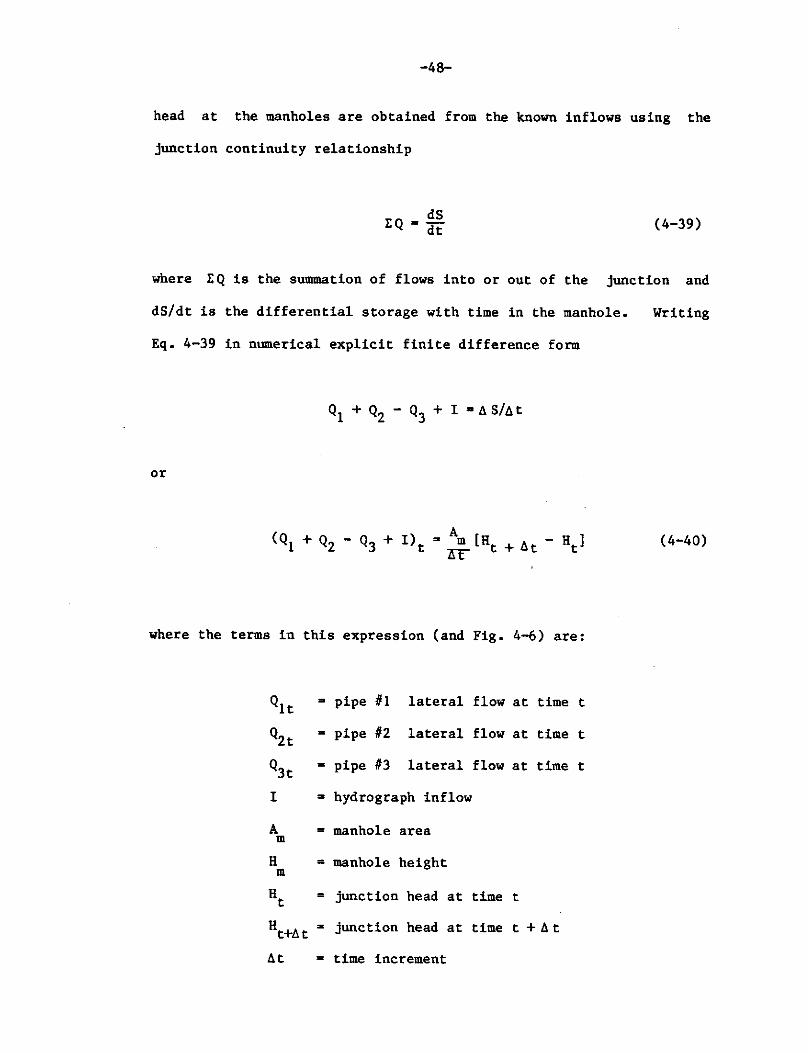
where the terms in this expression (and Fig. 4-6) are:
Qlt = pipe 111 lateral flow at time t
Q2t • pipe 112 lateral flow at time t
Q3t • pipe 113 lateral flow at time t
I = hydrograph inflow
A m = manhole area
H = manhole height m
Ht = junction head at time t
H • t+At junction head at time t +At
At = time increment
-49-
I
Am---._~11 Ht Ht+~t
Figure 4-6. Manhole (Junction) Boundary Conditions.
Rearranging Eq. 4-40 gives
(4-41)
in which Ht+at is computed using known values of head and flow at
time, t. Thus, each manhole with a variabl.e inflow has a known head
or boundary condition which is incorporated into the system equa-
tions.
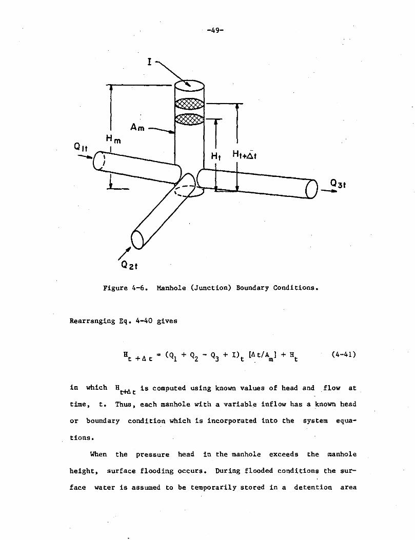
When the pressure head in the manhole exceeds the manhole
height, surface flooding occurs. During flooded conditions the sur-
face water is assumed to be temporarily stored in a detention area

As
H
-so-
Ds
T'----l"-------6 z
Datum
Figure 4-7. Flooded Manhole Conditions.
connected to the manhole and will return to the sewer system at a
later time without any volume loss. Surface flow routing is not
incorporated into the flow models.
Figure 4-7 shows a manhole with surface flooding conditons,
where:
D • manhole surface storage diameter s
A s manhole surface storage area s
Eq. 4-42 is modified to account for surface flooding by replacing the
manhole area A, with the surface storage area, A. m s
-51-
4.5 Initial Conditions
Numerical time schemes require that initial conditions concern
ing the dependent variable in the system equations be known. The
three numerical models developed in this thesis require that the
initial steady state values of head, H, and flow, Q, be known
throughout the entire system. These initial heads and flows are
obtained from a complete steady state flow analysis using a steady
state pipe network model (46).
The three numerical models are developed assuming that the
entire system or sub-system to be analyzed is under surcharge condi-
tions with each pipe flowing full. Therefore, each manhole in the
system will initially have a surcharged pressure head which depends
on the steady state flow in the pipes connecting the manhole.
4.6 System Equation Assembly and Assumptions
With the hydraulics of sewers developed mathematically in Chap
ter 3 and the hydraulics of sewer junctions or manholes described in
Section 4.4 a storm sewer network can be defined and analyzed. The
numerical models developed in Chapter 4 provide a method to .solve the
system equations based on a sewer link - junction node format. Thus,
at time t, the sewer network is simply disconnected at the manhole
junctions and the unknown values of pressure head and flow in each
link are solved independent of all other sewer links in the network.
This forms an independent set of p momentum equations, p line conti
nuity equations and j manhole or boundary equations where p is the
number of pipes in the system and j is the number of junctions or
manholes in the system. Upon solution of the link equations the
-52-
system is reassembled to allow for modifications of the manhole
boundary conditions for the next time step, t + I!. t. This procedure
is repeated over a finite period of time producing computed values of
pressure and head throughout the time simulation.
Nearly all numerical models which solve the governing unsteady
flow equations make use of a variety of assumptions which aid in the
solution of the system equations and the models developed herein are
no exception. The first assumption concerns the nature of the flow
during the time simulation. The analysis of surcharge storm sewer
flow is under investigation and therefore the models do not route
sewer flow under gravity or open channel· conditions. The models do,
however, predict small pressure heads which would indicate that
conditions are not suitable for pressurized flow.
Mathematically, it is difficult to make an exact energy analysis
of flow through a junction. Instead, approximate energy expressions
are assumed. In surcharged storm sewer systems, the manhole junc-
tions are considered submerged and losses are similar to those of
orifice flow with a head loss computed as 'rW2/2g. Mis a dimension
less head loss coefficient and Vis the instantaneous mean velocity
at the junction entrance or exit. For a sharp-edged entrance, M has
an approximate value of 0.5 and for an exit, Mis taken as 1.0. The
lumped parameter and steady state flow models allow for junction
energy losses through the use of minor loss coefficients as described
in Section 4.2 and 4.3.
The wall shear or frictional head losses in the manhole itself
are considered negligible since they are typically very small when
compared to the sewer line losses. Evaluation of other energy losses
-53-
in the manhole are only possible by relating them to line losses
using the minor loss equation.
The pipe line flow resistance equation in the Darcy-Weisbach
form is valid only for steady uniform flow. To this date, an un-
steady, nonuniform headloss equation is unknown. Thus, the finite
element and lumped parameter flow models incorporate steady state
head loss theory with the unsteady governing momentum and continuity
equations, Presently, this is an acceptable method for calculating
such losses since the flow variations occur slowly.
The final assumption concerns the treatment of surface flooding
near the manhole entrance, Detailed surface geometry of the land
above the sewer network is often unknown or unavailable and its
mathematical description is often difficult, The conditions imposed
by the models are described in detail in Section 4,4, However, it
should· be emphasized that surface flow routing between manhol.es is
not incorporated in the system equations. The surface water is
assumed to be temporarily stored in a basin area directly above the
manhole and will eventually return to the sewer system without volume
loss, This allows for accurate flood volume predictions in the area
of the manhole surface,
EXAMPLE PROBLEMS AND RESULTS
This chapter contains a comparison of the three hydraulic flow
models developed in Chapter 4 which analyze storm sewer systems
under peak flow conditions. Five examples are illustrated to show
the ability of each model to predict pressure and flow conditions in
systems under surcharge. The system geometry and properties are
presented for each example.
As discussed in section 4.5, the initial conditions for each
example are obtained from a steady state analysis of the storm sewer
system. These conditions are based on the assumption that the entire
system is flowing full under pressure.
Computer results are presented for each of the three models
developed. The values of hydraulic grade and flow are plotted with
time for each manhole and sewer line in the system. The dimension-
less coefficients, as discussed in Section 3.4, are also calculated
for each example.
The system coding instructions and typical computer output are
presented in Chapter 7.
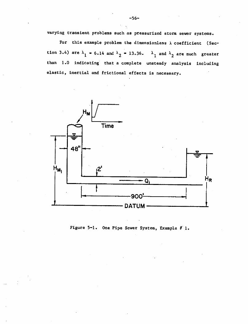
5.1 Example Problem!..!.
The system shown in Fig. 5-1 illustrates complete transient flow
in a single pipe sewer system. The 2 foot diameter, 900 foot long
sewer line transports storm water from a single 48 inch sewer manhole
to an outlet of fixed grade. The manhole input or source is in the
-54-

-55-
form of an input pressure-time variation shown in Fig. 5-2. This
pressure-time variation acts as a pressure forcing function at man
hole number 1, raising the manhole head from 15 feet to 60 feet in
0.5 seconds. This type of forcing function is required to cause
severe transients or pressure surges in a storm sewer system. For
simplicity the friction factor is assumed constant for the simulation
(f • 0.05645) and the pipe celerity (c) is 3000 feet per second.
The computer simulation results of example U 1 are shown in
Figs. 5-3 and 5-4. Four methods are presented. These include: a)
the wave plan model (47) b) the finite element distributed parameter
model c) the dynamic lumped parameter model and d) the steady state
with storage (kinematic) model. The hydraulic grade and flow values
are plotted with time for the pipe midpoint (450 feet from junction
1).
As shown in Fig. S-3, the oscillating pressure head is predicted
by the wave plan and finite element methods, which are complete un
steady distributed flow methods. Both the lumped parameter model and
the steady state model predict average hydraulic grades over the time
simulation. The pressure surges, created by the forcing function,
eventually dampen out with friction and tend to approach those of
steady state conditions.
Fig. S-4 illustrates the variable sewer flow over the time simu-
lation. As shown here, the dynamic lumped parameter model predicts
flow conditions which are similiar to the wave plan and finite ele-
ment models. This gives a preliminary indication that a dynamic
model, which includes inertial effects and neglects elastic consider
ations, may be appropriate for analyzing a certain class of slowly
-56-
varying transient problems such as pressurized storm sewer systems.
For this example problem the dimensionless A coefficient (Sec-
tion 3.4) are Al• 6.14 and A2
• 13.36. Al and A2 are much greater
than 1.0 indicating that a complete unsteady analysis including
elastic, inertial and frictional effects is necessary.
HM1 2'
O·
r· I . 90d . I DATUM
Figure 5-1. One Pipe Sewer System, Example u· 1.
60
-"C CJ 45 cu
::i:::
a,
0 .£:. c CJ
::E
15
-57-
0.5 1.0 2.0 3.0 4.0 5.0
Time, t (seconds)
Figure 5-2. Input Pressure-Time Variation for Example H 1.
-58-
I I I I I I
..... ·(I)
'ti :@
..... ..... (I) ... (I)
'ti i:: ..... 'ti :@ (I) (I) :@ = 'ti
(I) :@ i:: ..... ()
"' r:,J .... ..... () ... p. (I) ....
~· ... = (I) .... "' (I)
> i:: ~ i::
:m .... .... ~ Q :,.::
·--- -~------
0 0
U>
0 ... .. 0 o· .. 0 ... "'
0 0
PiU) c z D
0 <..I ... LI.I .en .,._
LI.I gx: .-NI-
0 ... . -0 0 . -0 ... 0
0 0
·s~.~~-oo~-0-,~~-oo~-s-E~~-oo~-o-E~~o-o-·-s-z~~o-o-·-o-z~~o-o-·-s-,---'L:._0_0_·4-oP C 133~1 0!13H
Figure 5-3. Total Head Graph for Junction 1.

"1 .... 00 i:: ... .. v, I ,,..
•
"1 ..... i G"l ... "' 'O ::,"
.... 0 ... "' ....
'O .. .... •
In "' 0 0
ci "' 0 0
II)
"' -Vlo u..o u· _o
"' Ulo .... 0 a: a: II) 3:" c ...J U..o
0
ci "
0 0
II)
0 0
r------------------------------------1 I I I I I I I I
. I I I I I I I I I I I I I
Wave Plan Model
Finite Element Mode_l
Dynamic Model
Kinematic Model ---------
°tld.-Q-Q~~~Q.-S-Q~~~l.rQ-Q~~-lr,5-Q~~-2~,-QQ~~-2T,-5Q~~-,~,-Q-Q~~,~.-5-Q~~~ •• ~Q-Q~~.~,.rs-Q~~-,5,QQ
TIME ISECCINDSl
I v,
"' I
-60-
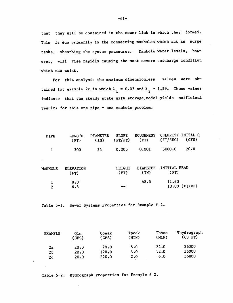
5.2 Example Problem J!..1
The system shown in Fig. 5-5 illustrates the effects of variable
inflow into a manhole of infinite height connected to a one pipe
storm sewer system. The system properties are shown in Table 5-1.
In order to determine the ability of each model to accurately predict
hydraulic grade and flow, the one pipe system is analyzed with three
different inflow hydrographs of equal volume. The hydrograph charac
teristics shown in Table 5-2, corrseponding to Fig. 5-6. With this
type of analysis, the system behavior is analyzed under various peak
flow conditions.
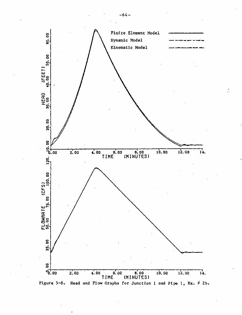
As shown in Figs. 5-7 through 5-9, the dynamic lumped parameter
solution yields results which are nearly identical to those of the
finite element distributed parameter model. The steady state solu
tion does not predict the pressure and flow oscillations, however, it
does predict accurate peak head and flow values at the correct point
in time. As the H-t and Q-t plots indicate, the true transient
solution tends to approach a stable steady state condition.
From this analysis and numerous other data runs, it is concluded
that severe pressure surges or transients are not a significant
problem in pressurized storm sewer systems under peak flow condi-
tions. Peak storm events, such as that in example Zc, may create
extended surcharge and flooding, however, pressure surges, as shown
in example 1, are not commonly found in completely pressurized sewer
systems under normal conditions. Only events such as two-phase flow
transitions and in-line pump failures cause significant pressure
surges. In the event that pressure surges do exist, it is likely
-61-
that they will be contained in the sewer link in which they formed.
This is due primarily to the connecting manholes which act as surge
tanks, absorbing the system pressures. Manhole water levels, how-
ever, will rise rapidly causing the most severe surcharge condition
which can exist.
For this analysis the maximum dimensionless values were ob-
tained for example 2c in which>. 1
= 0.03 and >..2
m 1.59. These values
indicate that the steady state with storage model yields sufficient
results for this one pipe - one manhole problem.
PIPE
l
LENGTH (FT)
300
MANHOLE ELEVATION (FT)
l 2
8.0 6.5
DIAMETER (IN)
24
SLOPE (FT/FT)
0.005
HEIGHT (FT)
ROUGHNESS (FT)
0.001
CELERITY INITAL Q (FT/SEC) (CFS)
3000.0 20.0
DIAMETER INITIAL HEAD (IN) (FT)
48.0 11.63 10.00 (FIXED)
Table 5-1. Sewer Systems Properties for Example# 2.
EXAMPLE Qin Qpeak Tpeak Tbase Vhydrograph (CFS) (CFS) (MIN) (MIN) (CU FT)
2a 20.0 70.0 8.0 24,0 36000 2b 20.0 120.0 4.0 12.0 36000 2c 20.0 220.0 2.0 6.0 36000
Table 5-2. Hydrograph Properties for Example# 2,
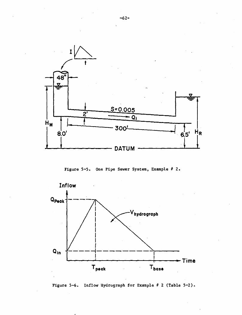
-62-
1D_ r•
-2'
S=0.005 Q;
I .. HM 300' ... / l HR 8.0' 6.5
1
l DATUM l l Figure 5-5. One Pipe Sewer System, Example# 2.
Inflow
QPeak
I I V hydro graph I I I I I I
------1-------------I I '--~~~ ....... ---------+-~----Time
Tpaak Tbase
Figure 5-6. Inflow Hydrograph for Example# 2 {Table 5-2).
Q Q
c "'
Q Q
Cc a:"' w :i:
Q Q
,,; -Q Q
-63-
Finite Element Model
Dynamic Model
Kinematic Model --------------
c-l-~~~~~~~~~~~-r-~~~-r-~~~-.--,--~~-.-~~~-r-~ 11.00 ,.oo 8.00 12.00 16.00 20.00 28.00
Q Q
c .,
Q Q'
24.00 TIME CMINUTESJ
c:\i+.-o-o~~-,~.~o-o~~~s~.-o-o~~-1~2~.-o-o~~-1~s-.o-o~~-2~0-.-a-o~~-2-,.-o-o~~-2-e-.-o-o-TIME (MINUTES)
Figure 5-7. Head and Flow Graphs for Junction 1 and Pipe 1, Ex.# 2a.
0 0
d IO
0 0
0 II)
... UJ UJ O u... 0 - . 0 .._
CJ a: 0 UJ O ::c: •
0 .,
0 0
d N
.,; N -0 0
d -o v,-u... u -0
0
.,; UJI'... a: a: 3:0 co ..Jo u... II)
0 0
.,; "'
0 0
2.00
-64-
Finite Element Model
Dynamic Model
Kinematic Model
•• 00 6. 00 8. 00 TIME (MINUTES!
9>~.-o-o~~-2~.-o-o~~-,~.-o-o~~-s~.-o-o~~-e~.-o-o~~-,~o-.-oo~~-,T2-.-oo~~-., •. TIME (MINUTES!
Figure 5-8. Head and Flow Graphs for Junction 1 and Pipe l, Ex.# 2b.
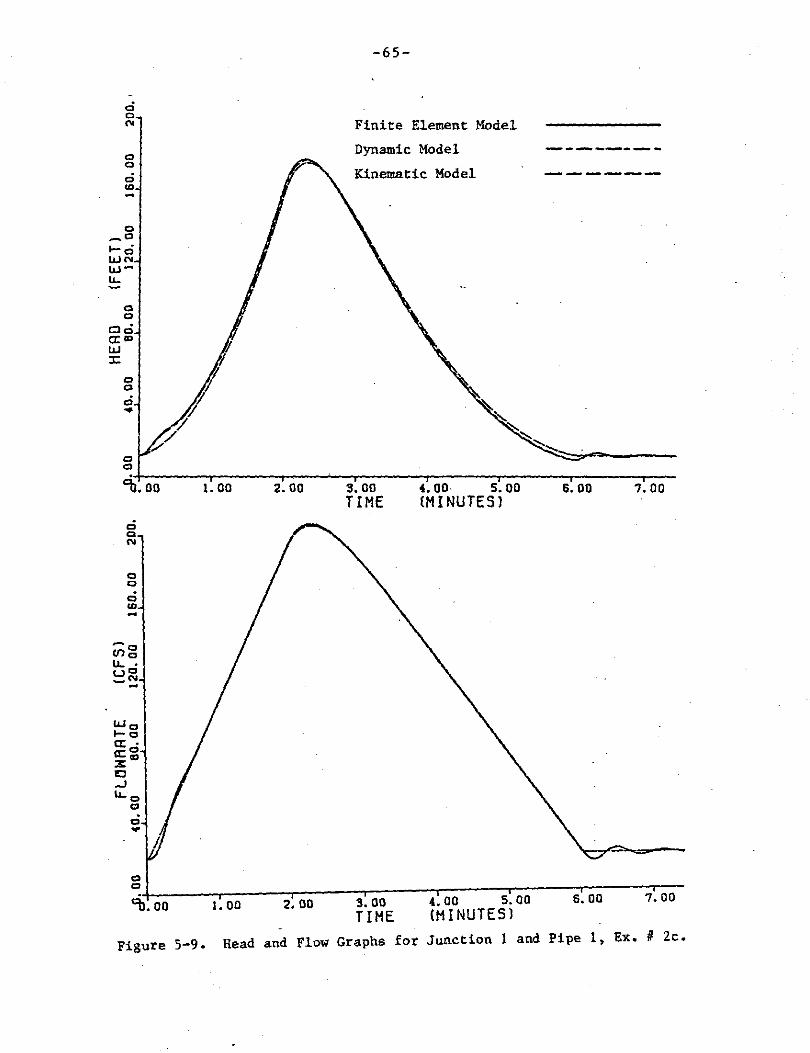
0 0
"' c:, 0
0 (0
0 0
oci a:"' LIJ ::c
0 0
0 .. 0 0
9i.oo
0 0
"' 0 0
Q ID -
-o trio u. • uo -"' -
0 0
"b. OD
!. 00
I, 00
2.00
2, 00
-65-
Finite Element Model
Dynamic Model
Kinematic Model
3.00 TIME
3.00 TIME
4. OD· S. 00 CM I NU TES J
4,00 5.00 CHINUTESJ
6.00 7.00
s. 00 7.00
Figure 5-9. Head and Flow Graphs for Junction 1 and Pipe 1, Ex.# 2c.
-66-
5.3 Example Problem !1
This five pipe storm sewer system illustrates the effect of
severe surcharge throughout the system including surface flooding at
several manholes. The system includes sewer pipes of different
lengths, diameters, and slopes as listed in Table 5-3 and shown in
Fig. 5-10. An additional component in this analysis is the introduc
tion of minor loss coefficients, which account for the manhole junc-
tion losses. For this example the entrance loss is taken as 0.5
while 1.0 is used for the exit loss. Concrete pipe is used with a
roughness of 0.001 feet. The system equations are solved using a 1.0
second time step.
Hydraulic grade (head) and flow graphs with time are presented
in Figs. 5-11 through 5-15. From this analysis, severe surface
flooding is seen to occur at manholes 1, 2 and 3 with minor flooding
at manhole 4. Flooding is a stabilizing factor in the analysis and
allows for extremely accurate predictions with the kinematic flow
model. However, as surface flooding subsides, and the water surface
recedes back into the manhole, the flow calculations are unstable
using the kinematic model. At this point only the dynamic model
accurately predicts the system pressures and flows. The kinematic
model consistently predicts average pressure and flow values through
out the instability.
In this example several situations occur in which the water
surface in the manholes drops below the pipe crown (eg. manhole 1 at
time • 21.0 minutes). This indicates a highly unstable two-phase
flow condition in which both pressurized and open channel flow co-

-67-
exist, The flow models developed herein, do not incorporate two-
phase flow and assume pressurized flow throughout the simulation,
A storm sewer network behaves as a system and the feedback
between parts of the network is directly shown in the results, In
this example, junctions 3 and 5 play key roles in determining the
system pressure and flow patterns throughout the simulation, A major
disturbance at time= 12,5 minutes at junction 3 (residing water
surface in manhole 3) causes severe flow disturbances at that same
time in all sewer lines connecting that junction, This cause and
effect relationship occurs whenever a substantial flow disturbance is
encountered during the simulation,
The dimensionless coefficient A2
has a value of 5,84. This
indicates that a dynamic flow analysis is desirable for this example
problem.
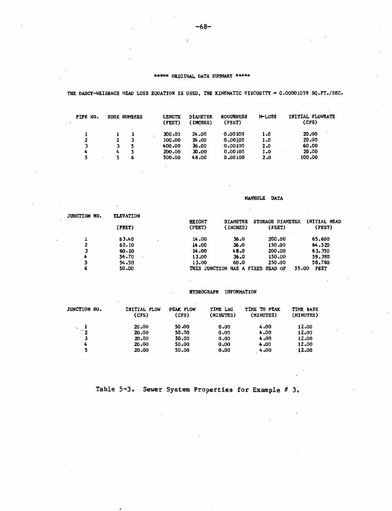
-68-
***** ORIGINAL DATA 5Ir.1KARY *****
THE DARCY-WEISBACH HEAD LOSS EQUATION IS USED, THE KINEMATIC VISCOSITY.• o.00001os9 SQ.FT./SEC.
PIPE NO.
I 2 3 4 5
JUNCTION NO.
I 2 3 4 5 6
JUNCTION NO.
I . 2
3 4 5
NODE NUMBERS
l 3 2 3 3 5 4 5 s 6
ELEVATION
(FEET)
63.40 62.10 6Q.IQ 56.70 54.SO 50.00
INITIAL FLOW (CFS)
20.00 20.00 20.00 20.00 20.00
LENGTH DlA11ETER ROUGHNESS !I-LOSS INITIAL FLOIIRATE (FEET) (INCHES) (FEET) (CFS)
300.00 24.00 0.00100 1.0 20.00 100.00 24.00 0.00100 1.0 20.00 400.00 36.oo 0.00100 2.0 60.00 200.00 JO.oo 0.00100 1.0 20.00 500.00 48.00 0.00100 2.0 100.00
MANHOLE DATA
HEIGHT (FEET)
DIAMETER STORAGE DIAMETER INITIAL HEAD (INCHES) (FEET) (FEET)
14.00 36.0 200.00 14.00 36.0 !SO.OD ·14 .oo 48 .o 200 .oo 13.00 36.0 150.00 13.00 60.0 250.00
THIS JUNCTION HAS A FIXED HEAD OF
HYDROGRAPH INFORMATION
PEAK FI.Oil TIME LAG TIME TO PEAK (CFS) (MINUTES) (MINUTES)
50 .oo o.oo 4 .oo 50.00 o.oo 4 .oo 50.00 o.oo 4.00 50.00 o.oo 4 .oo 50.00 o.oo 4.00
65.600 64 .520 63.350 59.380 58.780
55.00 FEET
TIME BASE (MINUTES)
12.00 12.00 12.00 12.00 12.00
Table 5-3. Sewer System Properties for Example# 3;
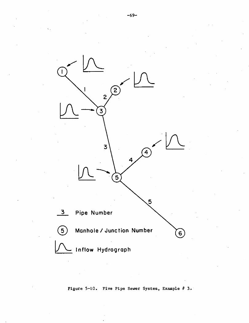
-69-
3 Pipe Number
® Manhole I Junction Number
~ Inflow Hydrograph
Figure 5-10. Five Pipe Sewer System, Example# 3.

-70-
d. ID
0 n 0 I . l(!· I - I I-
UJ I LIJo I U..o - . I 0 ... c a: 0 UJo ::c: • ' I\
"'· fO
0 0
d "b. 00 .: 00 a.oo 12.00 16.00 20.00
~-0 0
d ....
0 0 _.,_
en"' LI.. u -0
0
o. UJ"' I-a: a: %0 c,0
_J Iii. 11..N
0 0
o . ...
0 0
.,;
Dynamic Model
Kinematic Model
)
TIME (MINUTES)
v
• •
11. 00 a: oo 12. oo 16. oo TIME !MINUTESJ
A
20.00
24.00 28. 00
24,00 28. 00.
Figure 5-11. Head and Flow Graphs for Junction land Pipe 1, Ex.# 3.
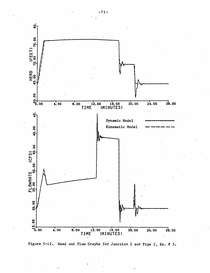
o . .. 0 0
f .,; . ... I- I UJ 1 UJo I U.c:> -o . I ... I 0 l a:c:, UJo :c .
II),
"' 0 Cl
0 "b.oo
.,;, .. Cl Cl
ci . .. 0 0
_ 11)_
u,"' u. u -0
0
ci
~ IJ.I "' I-a: 0: 3:0 co . -Jui. U.N
0 0
ci. N
0 0
.,; 11.oo
.: 00
.(.00
-71-
A •
II
-, , 8.00 12.00 16.00 20.00
TIME CHINUTESJ
I,. v •
Dynamic Model
Kinematic Model
v
I A. •• Ill' N
a: oo 12. oo . ts. oo 20. oo TIME CMINUTESl
• u.oo 28.00
-------
u.oo 28.00
Figure 5-12. Head and Flow Graphs for Junction Zand Pipe 2, Ex.# 3,
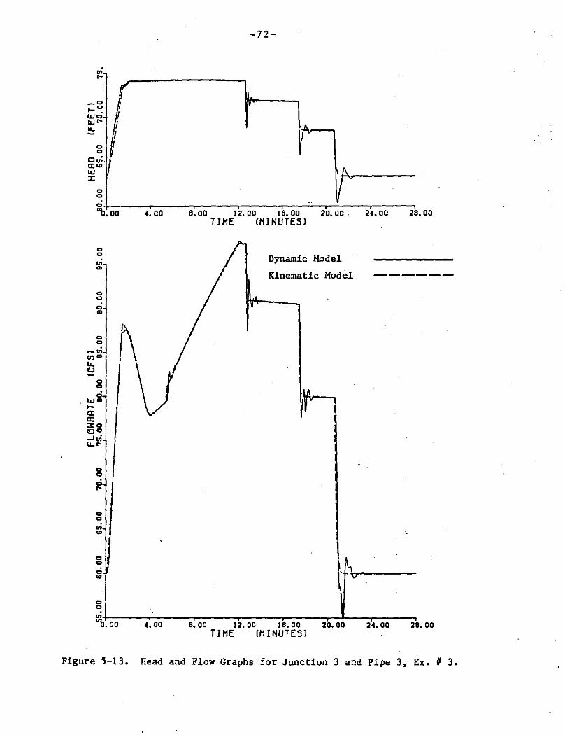
"' r-
.. .. c.,; a; .. .... :,: .. ..
.
.
.
( 1 1 1 1
0 "b.oo
.. ..
.,; ..
.. .. 0 m
.. .. _.,; "' .. "-~ .. ..
0 ...... .... a: cc 3:C> ,c<> -'in "- r-
.. .. 0 r-
.. ..
.,; ..
.. .. 0 .. .. .. .,; "b. 00
,. 00
4.00
-72-
' • .
/\ ,-.. . .
8. 00 12, 00 16. 00 20. 00 . 2,. 00 TIME !MINUTES)
Dynamic Model
Kinematic Model
8. oo 12. oo 1s. oo 20. oo TIME CMINUTESJ
24.00
' 28.00
28.00
Figure 5-13. Head and Flow Graphs for Junction 3 and Pipe 3, Ex.# 3.
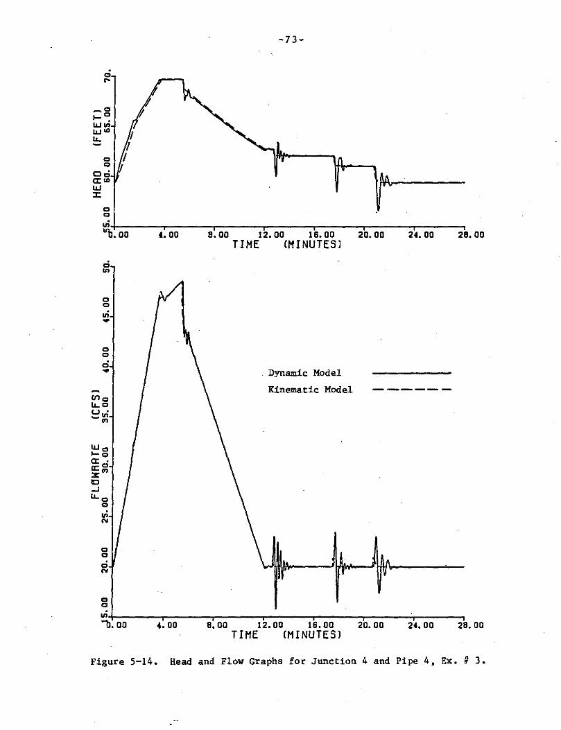
0 ....
0 0
Oci CC ID w ::c:
0 c:,
-73-
~+-~~~-.-~~~-.-~~~ ..... ~~~~.-~-.--.--,-................................... ~ ...... "b. DD «. DO 8. 00 12. DO 16. 00 20. 00 24. OD 28. DD
ci u,
0 0
~ .. 0 0
ci .. en o LI.. 0 u· _u. .,
Wo ._ c:, cc . a;:O x"' c -l Ll..o
0
.,; N
0 0
ci N
0 c:,
TIME !MINUTESJ
Dynamic Model
Kinematic Model
~+-~~-.-.....,... ...... ~~-.~~~~...-~~-.-...---.-~-.-..,....~-.-~ .............. ..,.... ...... ......, "'b. DO «. OD 8. DO 12. 00 16. DO 20. DO 24. OD 28. 00
TIME CMINUTESJ
Figure 5-14. Read and Flow Graphs for Junction 4 and Pipe 4, Ex.# 3.
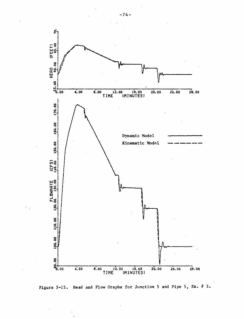
0 ...
Cl Cl
Oo a:<o IU :i::
Cl Cl
-74-
~-t-~~-,,--~~~~~~-r--~~--,,--~.::--.-~~~~--,~~ "b. 00 ,. 00 8. 00 12. 00 16. 00 20. 00 - 2(. 00 28. 00
Cl Cl
0 ... -Cl Cl
g -Cl Cl .,; .. -
Cl Cl
.,; --Cl 0 .,; 0 -0 0
TIHE (MINUTES)
Dynamic Model
Kinematic Model
.,;+-~~--,,----,--,~--,--,~~--,--,--,~--,~~----'--,~--,--,~~
°b.oo ,. 00 8.00 12.00 16.00 20.00 2(. 00 28. 00 TI HE CM I NUTES J
Figure 5-15. Head and Flow Graphs for Junction 5 and Pipe 5, Ex. H 3.

-75-
5.4 Example Problem f!..i
This seven pipe system shown in Fig. 5-16 is the largest system
analyzed and illustrates the time lag effect of storm events. The
system properties are shown in Table 5-4. For this system, different
inflow hydrographs with appropriate hydrograph time lags are applied
to each manhole. Manhole 5 represents a junction box connecting the
lateral sewer lines with a vertical drop inlet which restricts sur-
face inflow. Surcharge and surface flooding, however, are allowed
at this manhole. The total time of the simulation is 30 minutes with
a 0.5 second time step.
The hydraulic grade and flow values are plotted in Figs. S-17
through 5-23 for each manhole and sewer line respectively. Manholes
1,2,3,4, and 6 experience severe flooding while manholes S and 7
completely contain the surcharge within the system.
time lag of 1 (manhole 3,4) and 2 minutes (manhole
The hydrograph
5,6) directly
effects the flow patterns in the corresponding downstream pipes as
shown in Figs. 5-22 through 5-25.
As compared to example 3, this system has relatively stable
pressure and flow conditions throughout the simulation. The kinema-
tic solution yields very accurate results when compared to the dynam-
ic solution, This indicates that a steady state model may be used
for reliable predictions of maximum pressure and peak flows if small
time steps are used,
The dimensionless coefficient 1 2 has a maximum value of 0.23 for
this problem. This indicates the importance of the frictional forces
as compared to the body and inertial forces, For this reason the
75
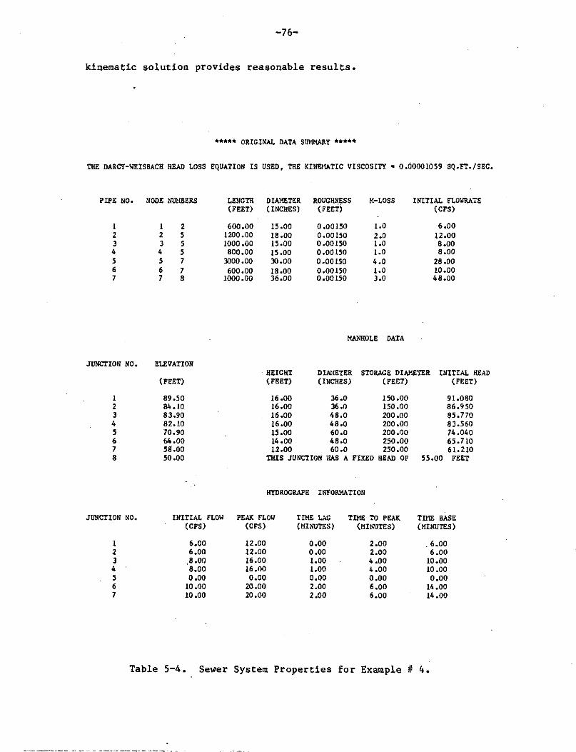
-76-
kinematic solution provides reasonable results.
**"'** ORIGINAL DATA SUMMARY*****
THE DARCY-IIEISBACH HEAD LOSS EQUATION IS USED, THE KINEIIATIC VISCOSITY• 0,00001059 SQ.FT./SEC.
PIPE NO, NODE NUMBERS LENGTH DIA.'1ETER ROUGHNESS M-LOSS INITIAL FLOW'RATE (FEET) (INCHES) (FEET) (CFS)
I I 2 600.00 15,00 0 .00150 1.0 6.00 2 2 5 1200.00 18.00 0.00150 2.0 12.00 3 3 5 1000.00 15.00 0.00150 1.0 s.oo 4 4 5 BOO.OD 15,00 0.00150 1.0 s.oo 5 5 7 3000.00 30.oo 0.00150 4.0 28.00 6 6 7 600.00 18,00 0 .00150 1.0 10.00 7 7 B 1000.00 36.00 0.00150 3.0 48.00
MANHOLE DATA
JUNCTION NO. ELEVATION HEIGHT DIAMETER STORAGE DIAMETER INITIAL READ
(FEET) (FEET) (INCHES) (FEET) (FEET)
I 89.50 16.00 36.0 150 .oo 91.080 2 84.10 16.00 36.0 150 .oo 86.950 3 83,90 16.00 48.0 200.00 85.770 4 82.10 16.00 48.0 200.00 83.560 5 70.90 15,00 60.0 200.00 74 .040 6 64.00 14.00 48.Q 250.00 65.710 7 58·.oo u.oo 60.0 250.00 61. 210 B 50.00 THIS JUNCTION HAS A FIXED HEAD OF 55.00 FEET
HYDROCRAPH INFORMATION
JUNCTION NO. INITIAL FLOII PEAK FLOW TIME LAG TIME TO PE...\K TUIE BASE (CFS) (CFS) (MINUTES) (MINUTES) (MINUTES)
I 6.00 12.00 o.oo 2.00 . 6.00 2 6.00 12.00 o.oo 2.00 6.00 3 8.00 16.00 1.00 4 .oo 10.00 4 8.00 16.00 1.00 4 .oo 10.00 5 o.oo o.oo o.oo o.oo o.oo 6 10.00 20.00 2.00 6.00 14.00 7 10.00 20.00 2.00 6.00 14.00
Table 5-4. Sewer System Properties for Example# 4.
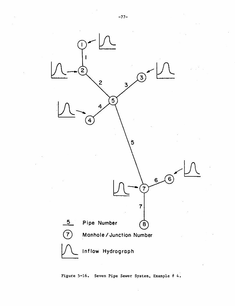
-77-
7
5 Pipe Number
0 Manhole I Junction Number
~ Inflow Hydrograph
Figure S-16. Seven Pipe Sewer System, Example# 4.
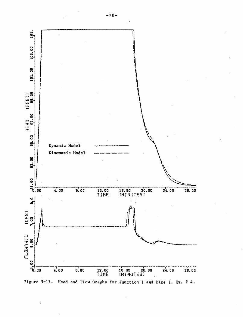
0 0
"' 0 -0 0 -0 -
0 0
0,.: a:"' w ::c:
-en
0 0
.,; 0,
0 0 ..;
"' 0 0
0
.;
II.. 0 uo - . ....
w .... 0 a: 0 IC ,
.x "' Cl -l II..
0 c:,
j
Dynamic Model
Kinematic Model
-78-
l I l I l l
I l I I I I
I
"b~.-o-o~~-.~.-o-o~~-e~.-o-o~~-1~2-.o-o~~-1~s-.o-o~~-2~0-.o-o~~-2~,-.o-o~~-2~e-.o~o TIME (MINUTES)
Figure 5-17. Head and Flow Graphs for Junction land Pipe l, Ex.# 4.

0 0
0 0
0 0
Co a: a,·
lJ.J :I:
0 0
"' a,
0 0
-79-
O..J--~~~-,.~~~~~~~~~~~~~,--~~~~~~~--..~~~~-,--
"b. 00
0 0
a,
(I') 0 I.L.O u . -~ lJ.J O 1-o a: . cc• 3:-c ...I I.L.o
0
r.i -0 0
4. 00 8. 00 12. 00 TIME
16. 00 20. 00 (MINUTES!
24. 00
Dynamic Model
Kinematic Model ------
28. 00
o+-~~~-.~~~~-.-~~~-,.~~~~~~~~~~~~~~~~~~-'o. 00 4. 00 8. oo 12. 00
TIME 16. 00 20. 00 24. 00 28.00 (MI NU TES J
Figure 5-18. Head and Flow Graphs for Junction 2 and Pipe 2, Ex. II 4.

ci Q -Q Q
a,
"' Q Q
..; "' Q Q .. "'
- . N
"'
Q Q
., a,
Q Q
ID a,
Q Q
Q -Q (fl •
u.. -u-
Dynamic Model
Kinematic Model
-80-
I I I I I
28. 00
Figure 5-19. Head and Flow Graphs for Junction 3 and Pipe 3, Ex.# 4.
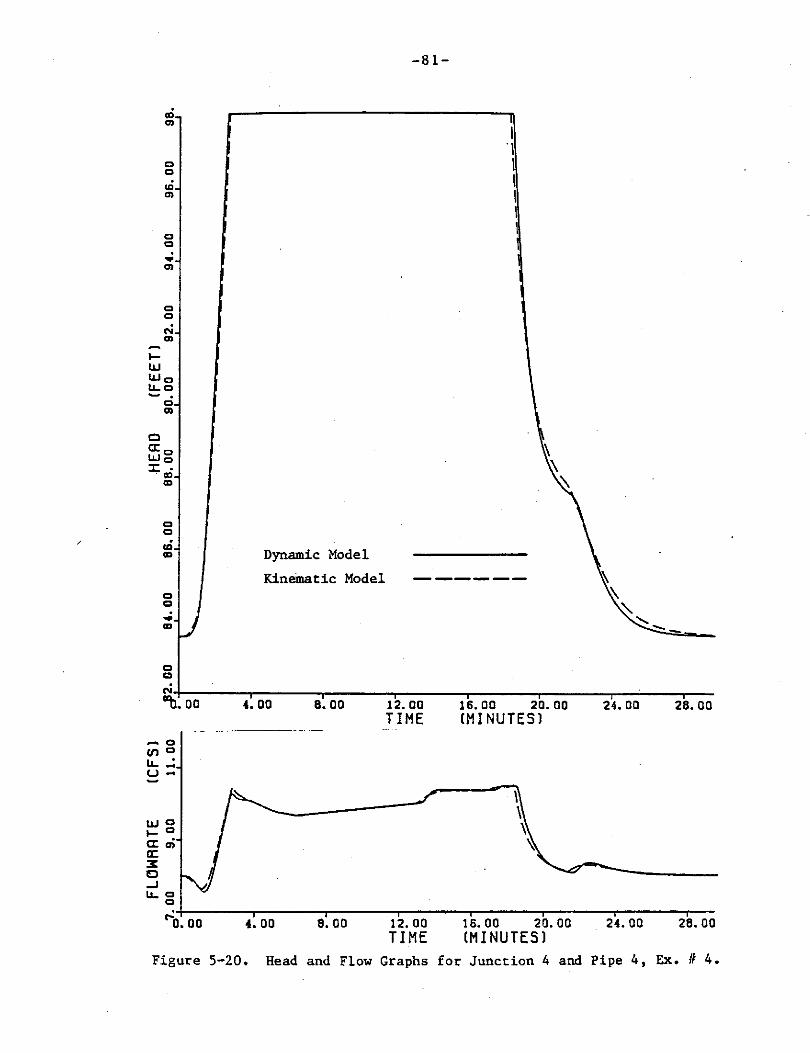
.; "' 0 0
U)
"' Q 0 .. "' 0 0 ,.. "'
1-UJ UJo "- 0 - .
0
"' c a:o Wo ::i:: • . ., .,
Q 0
.; .,
c, c, .. .,
c, c,
Dynamic Model
Kinematic Model
-81-
I 1 l I I
N-t-~~~-,-~~~-,-~~~--,~~~~.-~~~.,-~~~--,-~'--~-,-~ "b. 00
- 0 Vl O "- ..: u-
UJ Q I- Q
a: a; a: 3 Cl ..J "- Q
Q
4. 00 8. 00
----------
12. 00 TIME
16. 00 20. 00 CMI NUTESJ
\ \ 'i ~
24. 00 28.00
~o~.-o-o~~~.~.-oo~~~e~.-o-0~~~12~.-o-o~~-1~s-.-oo~~-2~0-.-o-o~~-2~4.-o-o~~-2~e-.~oo TI ME EM I NU TES I
Figure 5-20. Head and Flow Graphs for Junction 4 and Pipe 4, Ex. II 4.

.. "' 0 0
N
"'
0 0
Cl.; a:rLLJ :c
0 0
"' ....
0 Q .. ....
Q Q
Dynamic Model
Kinematic Model
-82-
N'+-~~~-r~~~~~~~-,~~~~,--~~~,-~~~-,-~~~-,.~ ""o. oo 4.00 8.00
.. "'
0 0
;;:; ~ u.. u
0 0
LL.IO I-"' a: a:: 3:0 Co ..J • u..~
0 0
12. 00 TIME
16. 00 20. 00 (MI NUT ES J
24.00 28.00
~-+-~~~-.-~~~-.-~~~~~~~~~~~~,-~~~-.-~~~-.-~ "ti. 00 4. 00 8. 00 12. 00
TIME 16. 00 20. 00 24. 00 28.00 (MINUTES)
Figure 5-21. Head and Flow Graphs for Junction 5 and Pipe 5, Ex.# 4.
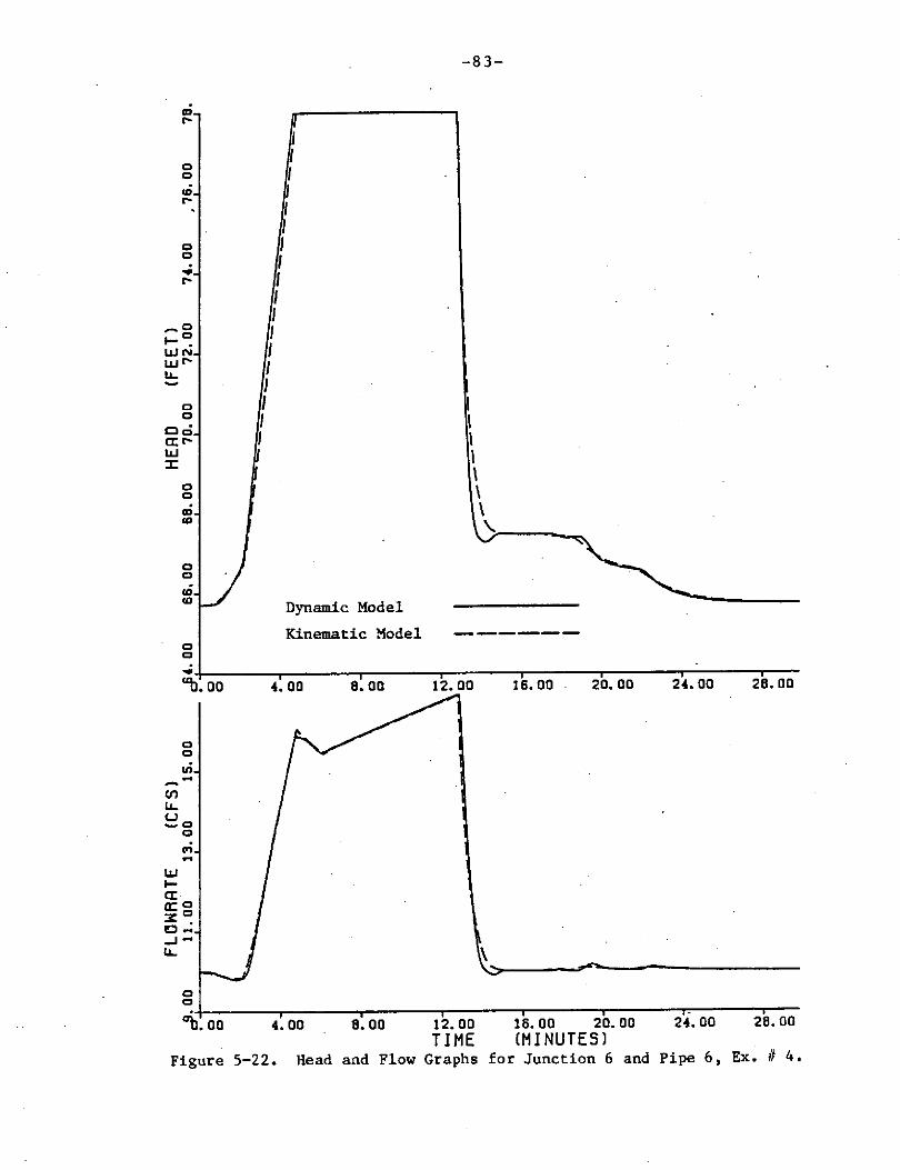
CD ....
0 0
"' ....
0 0 .. ....
0 0
oci a:rlLI :I:
-
0 0
.; IO
0 0
,,; "' 0 0
0 0
ui -(I')
IL. u -o
0
... -ILi .... a: a: 0 :z:O c..: ...1-IL.
0
I I I I I I I I I I I I I I I I I I
Dynamic Model
Kinematic Model
-83-
I I I I I \ \..
0-1-~~~ ...... ~~~......-~~~--,~~~~.---~~~-r-~~~.....,.,.~~~......-~-"b. 00 4. OD 8. 00 12. 00 16. 00 20. DO 24. 00 28.00
TIME CMINUTESJ Figure 5-22. Head and Flow Graphs for Junction 6 and Pipe 6, Ex.# 4,
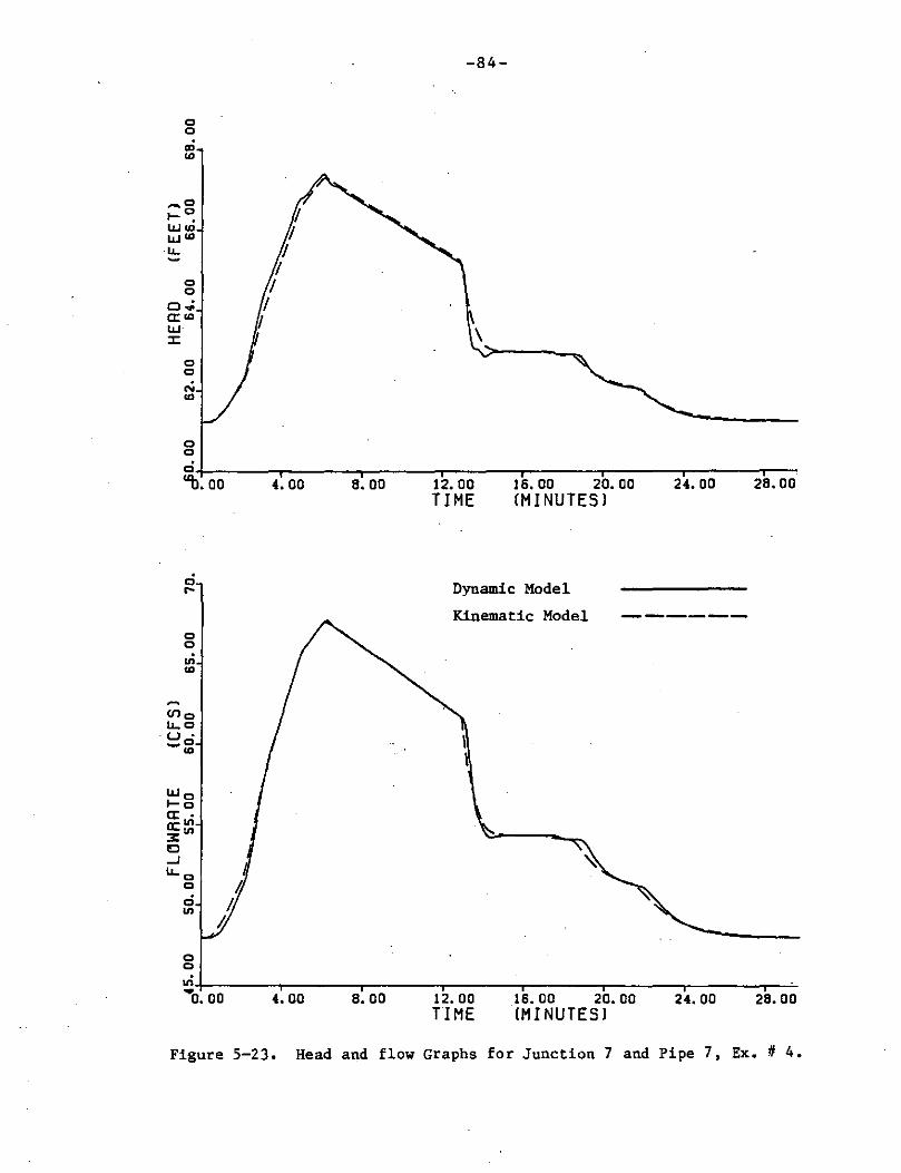
0 0
.,; co
0 0
... co
0 0
7 7
7 '/
'/ I
'/
-84-
\ \
o+-~~~...,..~~~ ...... ~~~--.~~~~....-~~~..-~~~...,..~~~-r~ "b. 00
0 ....
0 0
~ co
(l)o lJ.. 0 u . _o
co
Wo 1-o a: . a:"' :i::: "' c ...J lJ.. 0
0
0 "'
0 0
I,
I, !.
4. 00 8.00 12. 00 TIME
16. 00 20. 00 IM I NU TES l
Dynamic Model
Kinematic Model
I I
24. 00 28.00
~+-~~~-,-~~~ ..... ~~~--,~~~~....-~~~..-~~~~~~~~~~ •o. oo 4.00 0. oo 12.00
TIME IS. 00 20. 00 24.00 28.00 IM I NUT ES J
Figure 5-23. Head and flow Graphs for Junction 7 and Pipe 7, Ex.# 4.
-85-
5.5 Example Problem H 5
Example H 5 is a 3 sewer line system shown in Fig. 5-24. The
system includes sewer pipes of various lengths, diameters and slopes
as listed in Table 5-5.
roughness of 0.001 feet.
Concrete sewer lines are illustrated with a
The manhole and inflow hydrograph proper-
ties are also shown in Table 5-5.
This 3 pipe storm sewer system is relatively very flat with pipe
slopes ranging from 0.001 ft/ft to 0.002 ft/ft. Systems, such as
this, generally have substantial surcharge and flooding problems and
are often physically and numerically unstable. This is due primarily
to the small difference in head between adjacent manholes resulting
in unstable flowrates. In addition, this small potential head tends
to minimize the system flows resulting in larger storm detention and
increased chance of surface flooding. These factors make this 3 pipe
system ideal for testing the stability of the three flow models with
respect to the time step ( t; t) used.
The 3 pipe system is analyzed using the unsteady (transient),
dynamic, and kinematic (steady) models in order to determine the
relative numerical stability of each model. The finite element
distributed parameter model is assumed to provide the most reliable
and accurate solution. The maximum time step allowed is 0.0667
seconds (200ft/3000 ft/s) therefore t;t = 0.05 seconds and t;x = 10.0
feet are used for the finite element distributed parameter solution.
The dynamic and kinematic models are each tested for time steps ( 6t)
of 0.1, 1.0 and 5.0 seconds.
The results of hydraulic grade (head) and flow for each run are
-86-
plotted for comparison in Figs. 5-25 through 5-31 • For this prob
lem the kinematic model using time steps of 1.0 and 5.0 seconds
becomes unstable at time t • 11 minutes, producing oscillating posi
tive-negative values of flow for each time step. Kinematic solutions
for tt • 1,0 and 5.0 seconds are not shown in Figs. 5-25 to 5-31
because of the severe instabilities.
An analysis of the solution plots indicates th.e highly unstable
nature of flow for this system. Both the unsteady and dynamic models
yield similar results for small steps (at~ 1.0), The dynamic
solution for at• 5,0 seconds provides good results for peak head
and flow predictions, however minor instabilities are encountered
when manhole surcharge subsides (11 it~ 15 minutes), As expected
the kinematic solution, with at• 0,1 seconds, provides reliable
predictions of head and flow values throughout the time simulation.
For periods of unstable flow (t ~ 11 minutes), the kinematic model
predicts average values of head and flow in each manhole and sewer
line.
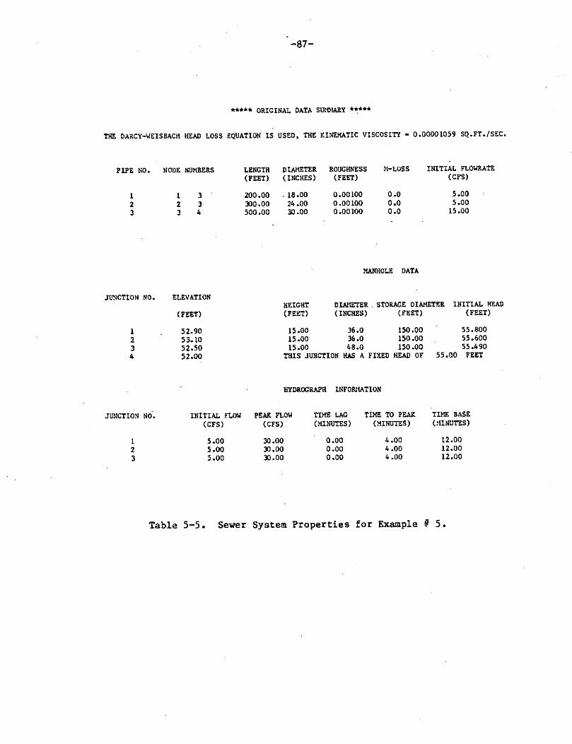
-87-
***** ORIGINAL DATA SUHMARY **:***
THE DARCY-WEISBACH HEAD LOSS EQUATION IS USED, THE KINEMATIC VISCOSITY• Q.00001059 SQ.FT./SEC,
PIPE NO,
I 2 3
JUNCTION NO.
I 2 3 4
JUNCTION NO·.
I 2 3
NODE NUMBERS
I 3 2 3 3 4
ELEVATION
(FEET)
52.90 53.10 52.50 52.00
INITIAL FLOW (CFS)
5.00 5.00 5.00
LENGTH DIAMETER ROUGHNESS M-LOSS INITIAL FLOWRATE (FEET) (INCHES) (FEET) (CFS)
200.00 . 18 .oo 0.00100 o.o 5.00 )'.)Q.00 24 .oo 0.00100 o.o 5.00 500.00 30,00 0 .00100 o.o 15.00
MANHOLE DATA
HEIGHT (FEET)
DIAMETER . STORAGE DIAMETP.R INITIAL IIEAD ( INCHES) (FEET) (FEET)
15,00 36.0 150.00 15 .oo 36 .o 150 .oo 15.00 48.0 150.00
THIS JUNCTION HAS A FIXED HEAD OF
HYDROGRAPH INFOR!IATION
PEAK FLOW TIME LAG TIME TO PEAK (CFS) (MINUTES) (MINUTES)
30.00 0.00 4.00 )'.),00 0.00 4.00 )'.).00 o.oo 4 .00
55.800 55.600 55 .490
55.00 FEET
TIME BASE (,UNUTES)
12.00 12.00 12.00
Table 5-5. Sewer System Properties for Example# 5.
-88-
3
2 Pipe Number
® Manhole/ Junction Number
~ Inflow Hydrograph
Figure 5-24. Three Pipe Sewer System, Example# 5,
Finite Element Model (At= 0.05 sec.) "1 0 .... 0 Dynamic Model (At= 0.1 sec.) ------------l)Q
:1 " Dynamic Model (At= 1.0 sec.) ... --------CD
v, Dynamic Model .(At= 5.0 sec.) ------I N
Kinematic Model (At= 0.1 sec.) v, 0 ....
'iJ rt .. 0 I ..... 0
;:i:; In 9( CD ID
t ~ .... " IJ.J I ... IJ.J O
I/ .. lLO 'g. - .
0 ID
l I\ I ....
I~ 00 0 ... 0 "' " I
<-, CCo
"' IJ.J O ::, :x:: • (> In rt "' .... 0 ::,
cl IVV .... 0
"' 0 x "' ~
"O ..... CD 0
0
"" In v, ... o: 00 • ,: 00 s:oo a:oo 10. 00 12.00 14.00 16.00 18.00 • 2.00
TIME !MINUTES!
..,, .... "" !; .. u,
,!, "' • ..,, .... ~ C') '1
"' "g. .... 0 '1
'"d .... ~ -"' x ~ "' .... .. "" u, •
c c c "' c c In "' c:, 0
-o Cll"' u.. u
c 0
In w-1-a: a: 3:c cO ..Jci u..-
0 0
"'
c c
9i. 00
Finite Element Model (6t = 0.05 sec.)
Dynamic Model (6t = 0.1 sec.) ------------Dynamic Model (6t = 1.0 sec,) --------Dynamic Model (6t = 5.0 sec.) Al-------Kinematic Model (6t - u., sec., ,.,, I
I
2.00 ,. 00 6.oo 8.oo 1b.oo TI ME CM I NUT ES I
---
! I
!~~~! 1 I
12. 00 14. 00 16. 00 18. 00
I
'° 0 I

Finite Element Model (At= 0.05 sec.) ":I .... Dynamic Model (At= 0.1 sec.) "" ------------" ... Dynamic Model (At= 1.0 sec.) 11> 0 --------
0 V1 ~l Dynamic Model (At= 5.0 sec.) I ------N ..... Kinematic Model (At= 0.1 sec.) .
)'/ ' el 'o 0 0 ... U1 Ill .... co
I /I v
' tr ~ _ci
"' I-~
... IJ,JO
Ill UJ co
'3- IL -gr· ,A/'AM I ..... "' 0 ..... ... i:::¥:!I I
c.... Cl.,; §
a: U1
UJ n :i::: ... .... 0 0 Cl ::> N
Cl U1
•
~ ~ 0
Cl
"' .,; .... 11> ... o: 00 2: 00 ,: 00 s:oo e:oo I il. 00 12.00 14.00 16. 00 18.00
"" TIME IM I NUT ES l V1 •
..,
.... (JQ
~ "' U1
.!,
"' .., ... 0 0: c;) ... I»
'"Cl ::r
"' 0 ... 'ti .... ~ N
t°'l x ~
'"Cl ... "' "" U1
d ..,
c 0
"' "' 0 0
c
"' (f)o u. 0 u . -~ ll.lo 1-o a: . a:~ :;:: 0 -' u.
0 0
Ill
0 0
d
0 0
Finite Element Model (6t = 0.05 sec.)
Dynamic Model (6t = 0.1 sec.)
Dynamic Model (6t = 1.0 sec.)
Dynamic Model (6t • 5.0 sec.)
Kinematic Model (6t = 0.1 sec.)
------------
----------
~;-~~~-r-~~~-r-~~~,-~~~,-~~~,-~~~.--~~~.--~~--,.---,,--~-, 10.00 2.00 t.oo s.oo e.oo 10.00 12.00 1t.oo 1s.tio 1e.oo
TIME !MINUTES)
I \0 N I
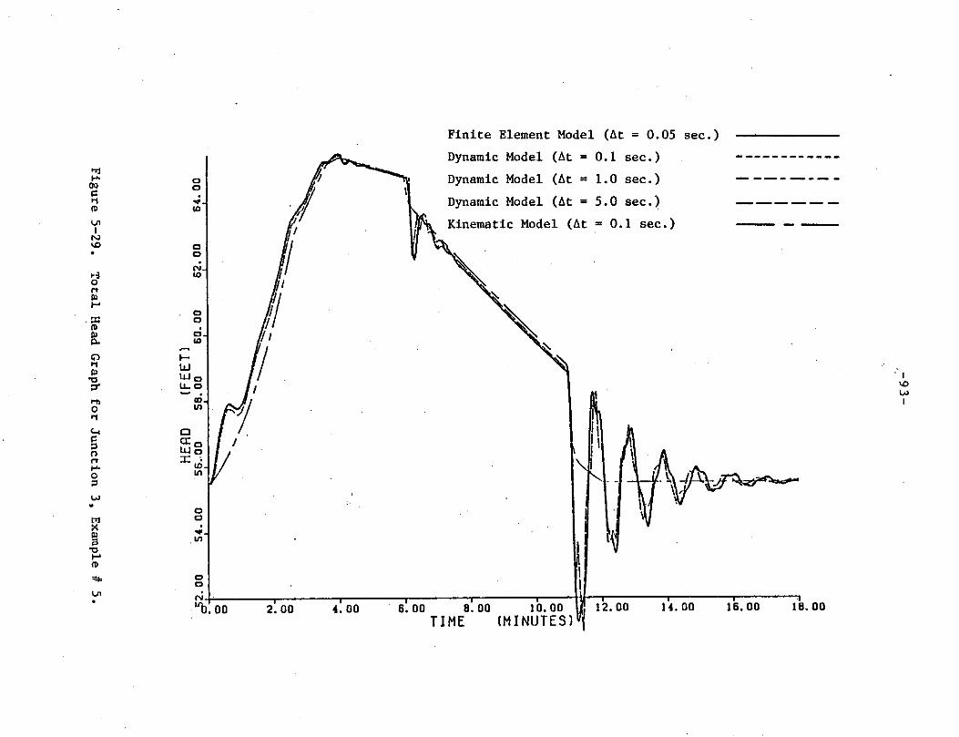
'<I 0 ..... 0 OQ
" ... ... (1) IO
v, I
N
"" 0 • 0
N •i ID 0 rt Ill ....
0 . :,: 0
(1) 0 ID [
~
(;) I-lJ.J ... lJ.J O
I"
LL.c 't:I ::r
"' Ul ..,, 0 ... c... CJ
CCo § lJ.J O :r: • " ID
rt Ul
.... 0 ;:,
..... . 0
trl 0
... ~
"' ~ 't:I .... (1) ... 0
0 ..,, N
"b; 00
?
·I "' v
2.00 4.00
Finite Element Model {6t = 0.05 sec.)
Dynamic Model (6t = 0.1 sec.)
Dynamic Model (6t = 1.0 sec.)
Dynamic Model (6t = 5.0 sec.)
Kinematic Model (6t = 0.1 sec.)
'
s: oo 8. oo 10. oo I~ 12. oo TIME IMINUTES)ll'j
14. 00 16. 00 18. 00
: I
"" ..., I

"l .... 00
" ....
"' "' I ..... 0 •
"l I-' 0 0:
"' ....
"' "CJ :,-
t-h 0 .... >'d ....
"CJ
"' w
l:>l x ~
"CJ I-'
"' "" "'
0
0 ...
0 0
0 "'
0 0
0 II)
(f)o IJ..O uc,; ~ .. UJo 1-o a: . a:~ 3: c ..J LL.o
0
0 N
0 0
0
0 0
Finite Element Model (6t = 0.05 sec.)
Dynamic Model (6t = 0.1 sec.)
Dynamic Model (6t = 1.0 sec.)
Dynamic Model (6t = 5.0 sec.)
Kinematic Model (6t = 0.1 sec.)
\I I
11
\
--------------
--
c:\i+.-o-o---2~.o-o---4~.-o-o---6~.o-o---a~.-o-o---1~0.-o-o--1~2-.-o-o--1~,-.o-o--~1s-.-o-o---,1a.oo TIME [MINUTES)
I
'° .,,.. I

CONCLUSIONS AND RECOMMENDATIONS
The primary objective of this thesis was to carry out a prelimi
nary investigation which would provide the basis for the eventual
development of a hydraulic flow model for the analysis of storm sewer
systems at peak flows. This investigation includes the initial
development of three hydraulic flow models. They are a) a finite
element distributed parameter unsteady flow model b) a dynamic
lumped parameter flow model and c) a kinematic steady flow model.
Comments on each of the flow models and future research recommenda
tions are presented here.
6.1 Finite Element Model
The unsteady distributed parameter finite element model provided
the most accurate and reliable solutions of the system continuity and
momentum equations. This method, however, by its distributed parame
ter nature, requires a large amount of computer storage and small
time steps for the even the simplest of system simulations. It is
not uncommon to find storm sewer systems in excess of 15 sewer links
of various lengths which may require the use of several hundred
elements. Each element in turn, has properties such as pipe length,
diameter, roughness, slope, celerity, etc. which must be stored
throughout the time simulation. Further complications arise with the
small time steps required for reliable solutions. Transient pressure
waves in pressurized storm sewer systems often travel in excess of
-95-
-96-
the speed of sound (3000 ft/s), In order to correctly model the
transient pressure waves the computational time step must not exceed
L /c, where s L is the minimum sewer element length in the sewer
s
system and c is the celerity or pressure wave velocity, For most
storm sewer systems, L /c is less than 0,1 seconds, s Many design
storms, however, exceed 20 minutes and would require in excess of
12000 time step calculations. Therefore, generally speaking, the
finite element solution or any distributed parameter solution applied
to pressurized storm sewer analysis (method of characteristics, wave
plan, etc.) may be computationally inefficient from a numerical
solution viewpoint,
The finite element model is also an implicit numerical model
which allows for a variety of time marching schemes. After thorough
investigation of the solutions and numerous unstable data runs it was
decided that the FEM yields inaccurate solutions for values of the
time weighting constant (e) less than 0,5, These accuracy problems
were anticipated considering the nature of the problem. According to
Zienkiewicz (54), the Euler explicit (6 =O) time marching scheme
often yields oscillatory or divergent results, From the author's
experience ,55 .$_6.$_ 0.8 yields satisfactory stable, nonoscillating
solutions, For this reason Galerkin weighting (0 = 0,67) is used for
all FEM solutions in this thesis,
Although not computationally appropriate for the analysis of
pressurized storm sewer systems, the FEM may well be applied to
general flow problems of fluid transients. These include both open
channel and closed conduit applications, Cooley and Mein (11) have
developed a FEM solution for open channel transients. However, after
-97-
a thorough literature search very little material has been published
concerning the application of the FEM to pressurized fluid tran
sients.
For future research it is recommended that a working finite
element model would provide a useful tool for the analysis of tran-
in closed conduits. With minor modifications, sients
finite element flow model developed herein, could be
the existing
modified to
handle routine transient flow problems, such as pump failures, value
closures, cavitation, etc. Particular attention would be given to
the spatial approximations and the non-linear flow resistant term.
Presently the FEM uses linear shape functions to describe spatial
variations of the unknown variables, Q and H. A more accurate quad
ratic, cubic or cubic hermitian approximation needs investigation.
The friction loss term is linearized in the present finite
element model and an alternate method of treating the friction term
is recommended. Possibilities include a modified Newton-Raphson
iteration procedure or a direct nonlinear solution of the governing
unsteady flow equations. One distinct advantage of the FEM would be
the quasi-steady modeling of the non-linear head loss term. The
friction loss for a given line length would vary over each element
allowing it to be an independent function of the nodal flow values.
Presently, several available transient flow models approximate the
friction loss based on the initial line flow. Consequently the head
loss is constant for a given line length throughout the entire simu
lation.
As with pressurized transients, the FEM could be easily applied
to the governing unsteady open channel flow equations for application
-98-
to sewer flow analysis. Such a model could then be coupled with the
present surcharged sewer model developed here to form a complete
finite element storm sewer analysis package. The FEM would provide a
useful alternative to the presently available numerical schemes.
6.2 Dynamic Model
The dynamic lumped parameter model provides a simple and reliab
le method for the analysis of storm sewer systems under surcharge.
As seen from the examples, the dynamic model yields accurate solu
tions for each problem investigated. From a computational viewpoint,
the dynamic model is comparatively efficient due to its lumped param
eter nature. In comparison to the kinematic model, the dynamic model
is much more stable and allows for the use of larger time steps (At).
In addition, the dynamic model, which includes inertial effects,
models unstable flow conditions quite well, whereas, the kinematic
model predicts mean values of head and flow throughout the instabili
fy.
The dynamic model is an explicit Euler ( e= 0) forward differ
encing time marching scheme. As previously indicated, the Euler
scheme often yields numerical instability problems for larger time
steps. For this reason, small time steps (At< 5.0 seconds) are used
for all simulations.
From this initial investigation, the dynamic lumped parameter
model provides stable and accurate results for the analysis of pres-
surized storm sewer systems. Additional research concerning the
numerical stability of the dynamic model needs to be conducted. With
minor modifications an implicit ( e~ 0) time marching scheme can be
-99-
developed for the dynamic model. This would allow for the use of
much larger time steps, thereby reducing the total number of calcula
tions and cost for each simulation.
With an implicit time marching scheme the boundary conditions
should also be modified accordingly. Because of the implicit nature
of these boundary conditions a modified Newton-Raphson iteration
procedure is recommended when solving for the unknown junction head.
6.3 Kinematic Model
The kinematic model is simply a time modified steady flow model
which predicts total head and flow values from previously known
steady state conditions. Of the three models presented, the kinemat
ic model is the simplest and most easily programmed. The solution
stability, however, is a significant problem. For very small time
steps (6t~ 1.0 seconds) the kinematic solution provides reasonable
results for each example investigated. For larger time steps, how-
ever, this method gives extremely unstable oscillatory results. For
this reason the dynamic model is preferred over the kinematic steady
flow model. Some improvements in stability may be possible if the
method for updating boundary conditions is modified. An implicit
procedure using a modified Newton-Raphson iteration technique is
suggested.
There are several advantages to the kinematic steady flow model.
Presently, steady state pressurized flow theory is well understood
and several well documented programs (46,31) are available which
analyze pressurized water systems. Although requiring small time
steps, the kinematic theory for pressurized storm sewer analysis
-100-
could be incorporated into these existing steady flow models. The
dynamic theory, which can not be adapted to the steady state models,
is not well documented or readily available at this time.
Presently Wood (46) has developed a extended steady flow model
which performs time simulations similiar to that of the kinematic
model presented here. The model is stable and accurate for pres-
surized storm sewer analysis, provided that small time steps are
used.
COMPUTER PROGRAMS
Two programs, called FESSA and DYN/KIN, are written for the
unsteady and dynamic/kinematic flow methods, respectively, developed
in Chapter 4. A description of the programs and data coding instruc-
tions for their use are presented in this chapter.
listed in Appendix I.
7.1 Fortran Programs
The programs are
FESSA, the finite element unsteady program was written and
debugged in Fortran IV, WATFIV and compiled and executed in Fortran
IV, G level. FESSA was initially programmed and run on the IBM-370
computer at the University of Kentucky. For additional versatility,
the program was transferred for execution to the DEC-10 computer at
the University of Louisville.
The dynamic and kinematic models are combined into one program,
called DYN/KIN, for execution and plotting convenience. For a pro
gram check the DYN/KIN program was written in both Fortran and Basic
computer languages. These programs are also executed on both the
IBM-370 and DEC-10 computer systems.
In each program the solutions of hydraulic head and flow are
stored in plotting arrays on either tapes or cards. These time solu
tions are then plotted using a Nicolet Zeta plotter by executing a
plotting program called PLTFLO written by the author. In producing
the plot, PLTFLO calls several plotting subroutines which are de-
-101-
-102-
scribed in the University of Kentucky Computing Center Plotting
Manual (36). PLTFLO is written and executed in Fortran IV, WATFIV on
the IBM-370 computer. The resulting graphical solutions of head and
flow are presented in Chapter 5.
7.2 ~ Coding Instructions
The data coding for the unsteady, dynamic and kinematic flow
models are very similiar. The coding consists of the original data
which describes the system geometry, an initial set of pressure and
flow conditions and optional plotting information. The data require
ments are summarized in Table 7-1 and 7-2 for the FESSA and DYN/KIN
programs respectively. In the data coding instructions, integer num
bers are represented by an 'I' followed by the ending column field
number and real numbers are represented by a 'R' followed by the
column field. All data fields are either l card column or a multiple
of 5 card columns. For example, (I:5) represents an integer variable
number which ends in card column 5 while (R:11-20) represents a real
number placed within card columns 11 through 20. Real variable num-
bers should contain a decimal for user convenience. Example data and
solution results are presented in Tables 7-3 through 7-6.
-103-
1. SYSTEM DATA (one card)
a) type of simulation, (1-unsteady, 2-dynamic); (1:1) b) number of sewer lines; (1:5) c) number of junctions/manholes; (1:10) d) time weighting constant; (R:11-20) f) time step, (seconds); (R:21-30) e) total simulation time, (minutes); (R:31-40) g) print time step, (minutes); (R:41-50) h) system kinematic viscosity, (sq-ft/sec); (R:51-60)
2. SEWER LINE DATA (one card for each pipe)
a) sewer pipe number; (1:5) b) connecting node# l; (1:10) c) connecting node# 2; (1:15) d) sewer pipe length, (ft); (R:16-25) e) sewer diameter, (ft); (R:26-35) f) sewer roughness, (ft); (R:36-45) g) initial sewer flow, (cfs); (R:46-55) h) sewer pipe celerity, (ft/sec); (R:56-65) i) element length, (ft); (R:66-75)
3. JUNCTION/MANHOLE/HYDROGRAPH DATA (one card for each)
a) junction number; (1:5) b) junction elevation, (ft); (R:6-15) c) number of connecting sewer pipes; (1:20) d) connecting sewer pipe numbers; (1:25,30,35,40,45)
aa) manhole type, (1-fixed head, 2-variable head); (1:1) bb) manhole height, (ft); (R:2-10) cc) manhole diameter, (inches); (R:11-20) dd) manhole surface area diameter, (ft); (R:21-30) ee) initial manhole head, (ft); (R:31-40)
aaa) initial hydrograph inflow, (cfs); (R:l-10) bbb) hydrograph peak flow, (cfs); (R:11-20) ccc) hydrograph time peak, (minutes); (R:21-30) ddd) hydrograph time base, (minutes); (R:31-40)
4. PLOTTING DATA (one card)
a) number of plots; (1:5) b) plot time step, (seconds); (R:6-10) c) time-axis increment, (minutes); (R:11-15) d) initial head-axis value at time a 0, (ft); (R:16-20) e) head-axis increment, (minutes); (R:21-25) f) flow-axis increment, (cfs); (R:26-30) g) sewer pipe/junctions numbers for flow/head plots; (1:35,40,
45,50,55)
TABLE 7-1. Data Coding Instructions for FESSA Program.
-104-
1, SYSTEM DATA (one card)
a) number of sewer lines; (I:5) b) number of junctions/manholes; (I:10) c) time step, (seconds); (R:11-20) d) print time step, (minutes); (R:21:30) e) total simulation time, (minutes); (R:31-40) f) system kinematic viscosity, (sq-ft/sec); (R:41-50)
2, SEWER LINE DATA (one card for each pipe)
a) sewer pipe number; (I:5) b) connecting node U l; (I:10) c) connecting node U 2; (I:15) d) sewer pipe length, (ft); (R:16-25) e) sewer diameter, (ft); (R:26-35) f) sewer roughness, (ft); (R:36-45) g) sewer minor loss; (R:46-55) h) initial sewer flow, (cfs); (R:56-65)
3, JUNCTION/MANHOLE/HYDROGRAPH DATA (one card for each)
a) junction number; (I:5) b) junction elevation, (ft); (R:6-15) c) number of connecting sewer·pipes; (I:20) d) connecting sewer pipe numbers; (I:25,30,35,40,45)
aa) manhole type, (I-fixed head, 2-variable head); (I:l) bb) manhole height, (ft); (R:2-10) cc) manhole diameter, (inches); (R:11-20) dd) manhole surface area diameter, (ft); (R:21-30) ee) initial manhole head, (ft); (R:31-40)
aaa) initial hydrograph inflow, (cfs); (R:1-10) bbb) hydrograph peak flow, (cfs); (R:11-20) ccc) hydrograph time lag, (minutes); (R:21-30) ddd) hydrograph time peak, (minutes); (R:31-40) eee) hydrograph time base, (minutes); (R:41-50)
4, PLOTTING DATA (one card)
a) number of plots; (I:5) b) plot time step, (seconds); (R:6-10) c) time-axis increment, (minutes); (R:11-15) d) initial head-axis value at time= O, (ft); (R:16-20) e) head-axis increment, (minutes); (R:21-25) f) flow-axis increment, (cfs); (R:26-30) g) sewer pipe/junctions numbers for flow/head plots; (I:35,40,
45,50,55)
TABLE 7-2, Data Coding Instructions for DYN/KIN Program,
0 .. .. ....
0 ....
0
"'
" "
0 .. .... " .. ! zO .... i ..
"'
0
"'
.. N
• • -<. < ' '
-
I
...
I
"1
' T <l
~ '
"' "
- -<
'
... - WI •
' ' '
- "' "
-
Table 7-3.
I-,.
...
-105-
1-. . t '
·-'-
I
' '
I I I
~-! I I
'
I
'
'
I
' i I ' ' I I \..) - ' ' .....
,I .. "" • - • - " _, u
I ' I ' ' I I ' - ' "'' ' ' ' c ~, c I '
' ., " I I - ~
_, I ' - " ' ' I ' I I
' ! I <l, I I I ' I
I ' ' ' ' ' ~., 0 <> I I I .. 0 I ' ,
"' u ' ' "' ,- .,, ' ... I I ' I " I <. ' ' . '
J ' ' I
' "" . ,-'- ' I c I I
.... I c, I ' I •• 1--
-· - 0 ( ...
i I ., I T I .; I
Example FESSA Data Coding for Example# 3.
-106-
0 .. I
t-t-+-+-+-+--+--+--+--+--+--t---+---+--+-+--+--+~1--1--1--+-+-+-+--+--+--f--.. .. 0 ..
-;-.. .. 0 ... I ~
0 f ... c
.. ., ., in ~ .. 0 z .. .. ., 0 c c
"" c ... _, •' 0 0 ... ., ., ., c ,. .... .,
"' c ' • • m 0 "' "" 9, :, ... .. .. z
zO "' ... ~ .. ( ' ... !I! .J 0 < 0 ., u
( '. < .. " < ' < z "' " u
i5 "" 0 Q u . ' ., ' . ' 1! " .... ' < '" u "" g 0 N
"' ' c '
if\ N "' " <.. ( .. "' < "'
< ( ' -.: ' " 0 u u
--, ' ' - - c -0 N '- ( <
' ' ' ' N
' !!! "' "'
..,. '
' ' 0 ' 7' '.
_, ' I I I
"' c c I I I
c "" "' .... ~. IN 2 - N,
·• ..., N i ' • u ll I I c- I ,-.: ' 0 I I .. "'
_,.., I No ., " "" .10 •• I "' u I
I I t-
'7' 0 T ' ., I I I I I
"' •• I tl u T _,
"" I I .. z
Table 7-4, Example DYN/KIN Data Coding for Example# 3.
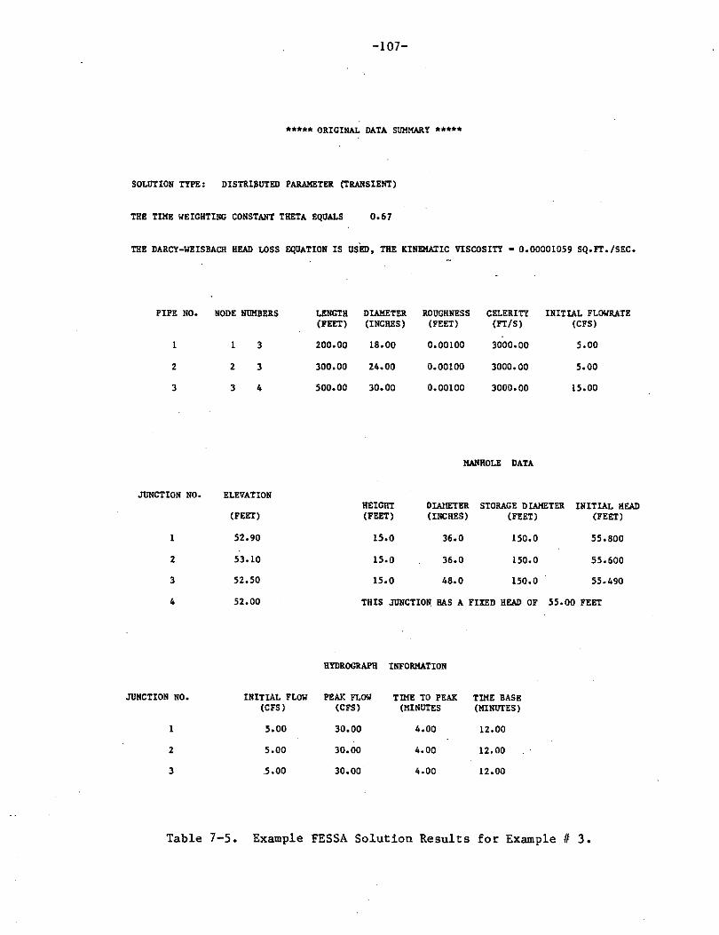
-107-
***** ORIGINAL DATA SUMMARY*****
SOLUTION TYPE: DISTRIJUTED PARAMETER (TRANSIENT)
THE TIME WEIGHTING CONSTANT THETA EQUALS 0,67
THE DARCY-WEISBACH HEAD LOSS EQUATION IS USED, THE KINEMATIC VISCOSITY - 0,00001059 SQ,PT,/SEC,
PIPE NO. NODE NUMBERS
1
2
3
JUNCTION NO.
1
2
3
4
JUNCTION NO.
1
2
3
1 3
2 3
3 4
ELEVATION
(FEET)
52,90
53,10
52,50
52,00
INITIAL FLOW (CFS)
S,00
5,00
s.oo
LENGTH DIAMETER ROUGHNESS CELERITY INITIAL FLOIIRATE (FEET) (INCHES) (FEET) (FT/S) (CFS)
200,00
300,00
500,00
18,00
24.00
30,00
HEIGHT (FEET)
15,0
15,0
15,0
0,00100
0.00100
0.00100
3000,00
3000,00
3000,00
MANHOLE DATA
DIAMETER STORAGE DIAMETER (INCHES) (FEET)
36,0 150,0
36,0 150,0
48,0 150,0
5,00
5,00
15,00
INITIAL HEAD (FEET)
55,800
55,600
55,490
THIS JUNCTION HAS A FIXED HEAD OF 55,00 FEET
HYDROGRAPII INFORMATION
PEAK FLOW TIME TO PEAK TIME BASE (CFS) (MINUTES (MINUTES)
30,00 4,00 12.00
30,00 4,00 12.00
30,00 4,00 12.00
Table 7-5. Example FESSA Solution Results for Example# 3.
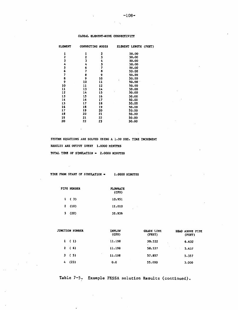
-108-
GLOBAL BLEMENT-!!ODE CONNECTIVITY
ELEMENT CONNECTING NODES ELEMENT LENGTH (FEET)
1 1 2 50.00 2 2 3 50.00 3 3 4 50.00 4 4 5 50.00 5 6 7 50.00 6 7 8 50.00 7 8 9 50.00 8 9 10 50.00 9 10 11 50.00 ·
10 11 12 50.00 11 13 14 50.00 12 14 15 50.00 13 15 16 50.00 14 16 17 50.00 15 17 18 50.00 16 18 19 50.00 17 19 20 50.00 18 20 21 50.00 19 21 22 50.00 20 22 23 50.00
SYSTEM EQUATIONS ARE SOLVEO USING A 1.00 SEC. TIME INCREMENT
RESULTS ARE OUTPUT EVERY 1.0000 MINUTES
TOTAL TIME OF SIMULATION• 2.0000 MINUTES
TIME FROM START OF SIMULATION • 1. 0000 MINUTES
PIPE NOIIBER FLOWRATE (CFS)
( 3) 10.951
2 (10) 11.010
3 (20) 32.936
JUNCTION NUMBER INFLOll GRADE LINE (CFS) (FEET)
1 ( 1) 11.198 59. 532
2 ( 6) 11.198 58.537
3 ( 5) 11.198 57.857
4 (23) o.o 55.000
HEAD ABOVE PIPE (FEET)
6.63?
5.437
5.357
J.000
Table 7-5. Example FESSA solution Results (continued).
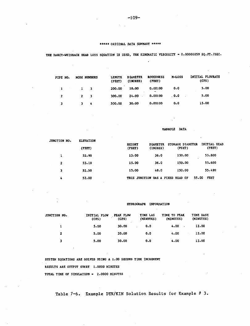
-109-
***** ORIGINAL DATA SUMMARY*****
THE DARCY-WEISBACH HEAD LOSS EQUATION IS USED, TBE KINEMATIC VISCOSITY • 0.00001059 SQ.FT./SEC.
PIPE NO. NODE NUMBERS
1 1 3
2 2 3
3 3 4
JUNCTION NO• ELEVATION
LENGTH DIAMETER ROUGHNESS M-LOSS (FEET) (INCHES) (FEET)
200.00 18.00 0.00100 o.o
300.00 24.00 0.00100 . o.o
500.00 30.00 0.00100 o.o
MANHOLE DATA
INITIAL FLOWRATE (CFS)
5.0D
5,00
15,00
HEIGHT DIAMETER STORAGE DIAMETER INITIAL READ (FEET) (FEET) (INCHES) (FEET)
1 52.90 15.00 36.0 150.00
2 53.10 15.00 36.0 150.00
3 52.50 15.00 48.0 150.00
4 52.00 TBIS JUNCTION HAS A FIXED READ OF
HYDROGRAPH INFORMATION
JUNCTION NO. INITIAL FLOW PEAK FLOW TIME LAG TIME TO PEAK (CFS) (CFS) _(MINUTES) (MINUTES)
1 5.oo 30.00 o.o 4.00
2 s.oo 30.00 o.o 4.00
3 s.oo 30.00 o.o 4.00
SYSTEM EQUATIONS ARE SOLVED USING A 1.00 SECOND TIME INCREMENT
RESULTS ARE OUTPtrr EVERY 1. 0000 MINtrrES
TOTAL TIME OF SIMULATION• 2.0000 MINtrrES
(FEET)
55.800
55.600
55.490
55.00 FEET
TIME BASE (MINUTES)
12.00
12.00
12.00
Table 7-6. Example DYN/KIN Solution Results for Example# 3.

~ II> TillE FROM START OF SIMULATION• er 1.0000 MINU'fKS ,_. .. ..... I
0-. ***** SOLUTION TYPE *****
~ m "' STEADY STATE W/STORAGE LUMPED PARAMETER ,_. "' "' PIPE NUMBER VELOCITY FLOW RATE VELOCITY FLOWRATE ~ (FT/SEC) (CFS) (FT/SEC) (CFS) --~ H 1 15.069 26.630 6.188· 10.935 z
I
"' 2 15.109 47,467 3,501 10.998 ... ... 0 0
,_. I " 3 o.638 3.130 6.696 32.870 ,.., ....
0
" : (I)
" ,_. JUNCTION NUMBER INFLOW GRADE LINE HEAD ABOVE PIPE GRADE LINE HEAD ABOVE PIPE ,..,
"' (CPS) (PEET) (FEET) !FEET) (FEET) ~
n 0
1 11.15 63.537 10.637 59.506 6.606
" 11, 15 64.039 10.939 58.524 S.424 ,.., 2 .... " 3 ll.15 55.024 2.524 57.839 5.339 " "' "" ~ 4 o.o 55.000 3.000 55.000 3.000
l 2 3 4 5 6 7. 8 9
10 11 12 13 14 15 16 17 18
c c c c c c c c c c c c c c c c c c c c c c c c c c c c c c c c c c c c c c
APPENDIX A ~ FORTRAN SOURCE PROGRAM
* ***** *** ** ••••• ******* •••••••••• ** •••• * •.•••• * •••••••••••••••• ****** * ················································~···················· • • • • • • ( FINITE ELEMENT SURCHARGED STORMSEWER i:.NALYSIS )
• • • • • •
• • • • * THIS PROGRAM SOLVES THE GOVERNING DIFFERENTIAL EQUATIONS FOR ONE* * DIMENSIONAL UNSTEADY (TRANSIENT) FLOW IN PRESSURIZED STORM SEWER* * SYSTEMS US HIG THE FINITE ELEMENT METHOD (FEM) • THE GALERKIN * * METHOD USING LINEAR ELEMENTS IS APPLIED IN ONE DIMENSIONAL SPACE.* • • • • • • • • • • • • • • • • • •
THESIS 1982
GREG c. HEITZMAN GRADUATE RESEARCH ASSISTANT
DEPARTMENT OF CIVIL Et<GINEERlllG UNIVERSITY OF KENTUCKY
• • • • • • • • • •
••••••••••••••••••••••••••••••••••••••••••••••••••••••••••••••••••••• •••••••••••••••••••••••••••••••••••••••••••••••••••••••••••••••••••••
IMPLICIT REAL*B(A-H,0-Z) REAL TPLOTM,HPLOTl,QPLOTl,HPLOT2,QPLOT2,HPLOT3,QPLOT3 REAL HPLOT4,QPLOT4,HPLOTS,QPLOT5 DIMENSION DATA(l),TPLOTM(l500),HPLOT1(1500),QPLOT1(1500) DIMENSION HPLOT2 ( 1500), QPLOT2 ( 1500), HPLOT3 ( 1500), QPLOT3 ( 1500) DIMENSION HPLOT4(1500),QPLOT4(1500),HPLOT5(1500),QPLOT5(1500) COMMON/Bl/NOPIPE,NOJUNC,TT,TTl,TINCR,VISC COMMON/B2/PNUM ( 111), JUNCl (HJ), JUNC2 ( 10) COMUON/B3/PLEN( 10), PDIA ( 10), PRUF ( 10), PFLO( 10), PCEL (10), PELEN( 10) COMMON/B4/JNUM(l0),JELV(l0),NOCP(l0),CPNUM(l0,5) COMMON/BS/KEY( 10), !lliT( 10), MDIAl ( 10), r!DIA2 ( 10), ,lllED (HJ) COMMON/B6/QI(l0),QIN(l0),QPK(l0),TPK(l0),TBAS(l0),TIME COMMON/B7 /JMOD(l0, 5) ,MPIPE(95 ).JUNC (95) C0t-1MON/B8/Q (9 5), H (95), /\MAT( 2, 2), Brll\T( 2, 2) COMMON/89 /ELEN( 95), EDIA( 95), ERUF ( 95), EFLO( 95), ECEL( 95), EALPHl\(9 5) COMMON/Bll /ID( 2, 95), HPBV (95) COM.MON/Bl2/IEL, NEQ, NEDF, NEND, NNDF, NOEL, MONO, LD( 4, 95), ~~ELCON ( 2, 95) COMMON/Bl3/SA,SF,SG
-111-
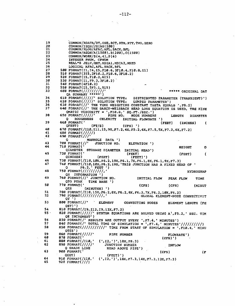
-112-
19 CoMMON/ROATA/DT,ONE,RCT,RTH,RTT,TWO,ZERO 20 COMMON/IEON/JDIAG(200) 21 COMMON/RLOG/AFAC,AFL,BACK,BFL 22 COMMON/REON/A(l500),B(200),C(l500) 23 COMMON/WORK/S(4,4),P(4) 24 INTEGER PNUM, CPNUM 25 REAL*S JELV,MHT,MDIA1,MDIA2,MHED 26 LOGICAL AFAC,AFL,BACK,BFL 27 500 FORMAT(Il,I4,IS,Fl0.6,3Fl0.4,Fl0.8,Il) 28 510 FORMAT(3I5,2Fl0.2,Fl0.6,3Fl0.2) 29 520 FORMAT(IS,Fl0.2,6I5) 30 530 FORMAT(Il,F9.2,3Fl0.2) 31 540 FORMAT(4Fl0.2) 32 550 FORMAT(I5,5FS.l,5I5) 33 600 FORMAT(//////////' ***** ORIGINAL DAT
QA SUMMARY*****') 34 610 FORMAT(/////' SOLUTION TYPE: DISTRIBUTED PARAMETER (TRANSIENT)') 35 620 FORMAT(/////' SOLUTION TYPE: LUMPED PARAMETER') 36 630 FO'lll1AT(//' THE TIME WEIGHTING CONSTANT THETA EQUALS ',F8.2) 37 640 FORMAT(//' THE DARCY-WEISBACH HEAD LOSS EQUATIOtl IS USED, THE KINE
QMATIC VISCOSITY• ',Fl0.8,' SQ.FT./SEC.') 38 650 FORMAT(/////' PIPE NO. NODE NUMBERS LENGTH DIAMETER
O ROUGHNESS CELERITY INITIAL FLOWRATE ') 39 660 FORMAT(' (FEET) (INCHES)
QFEET) (FT/S) (CFS) ') 40 670 FORMAT(/Il0,Ill,IS,9X,F7.2,4X,F5.2,6X,F7.S,5X,F7.2,6X,F7.2) 41 680 FORMAT(/////) 42 690 FORMAT(///'
O MANHOLE DATA ' ) 43 70!1 FORMAT ( / /' JUtlCTION NO. ELEVATION ') 44 710 FORMAT(' HEIGHT D
QIAMETER STORAGE DIAMETER INITIAL HEAD') 45 720 FORMAT(' {FEET) (FEET)
OINCHES) (FEET) (FEET)') 46 730 FO'lll-!AT(/Il0,10X,F6.2,19X,F6.l,7X,F6.l,8X,F6.l,9X,F7.3) 47 740 FORMAT(/Il0,10X,F6.2,19X, 'THIS JUNCTION HAS A FIXED HEAD OF
O F6.2,' FEET ') 48 750 FORMAT(//////////,' HYDROGRAP
OH ItlFORMATION ' ) 49 760 FORMAT(//' JUNCTION NO. INITIAL FLOW PEAK FL.OW TIME
OTO PEAK TIME BASE ' ) 5~ 770 FORMAT(' {CFS) {CFS) {MINUT
QES (MINUTES) ') 51 780 FORMAT(/Il0,15X,F6.2,8X,F6.2,8X,F6.2,7X,F6.2,10X,F6.2) 52 790 FORMAT(//////////,' GLOBAL ELEMENT-NODE CONNECTIVIT
OY 'l 53 800 FORMAT(//' ELEMENT CONNECTING NODES ELEMENT LENGTH (FE
OET) ') 54 810 FO'lll1AT(/I9,Il2,I9,13X,F7.2) 55 · 820 FORMAT(/////' SYSTEM EQUATIONS ARE SOLVED USING A;,F5.2,' SEC. TIM
OE INCREMENT') 56 830 FORMAT(/' RESULTS ARE OUTPUT EVERY ',F7.4,' MINUTES') 57 840 FORMAT(/' TOTAL TIME OF SIMULATIOtl • ',F7.4,' MINUTES'//////////) 58 850 FORMAT(///////////' TIME FROM START OF SIMULATION= ',Fl0.4,' MINU
OTES') 59 860 FORMAT(/////' PIPE NUMBER FLOWRATE') 60 870 FORMAT(' {CFS)') 61 880 FORMAT( /!10, ' ( 1
, I2,') ', 18X, FB. 3) 62 890 FO'lll·!AT(/////' JUNCTION NUMBER INFLOW
O GRADE LINE HEAD ABOVE PIPE') 63 900 FORMAT(' . (CFS) (F
OEET) (FEET)') 64 910 FOR11AT(/Il0,' ( 1 ,I2,•) 1 ,l8X,F7.J,14X;F7.3,13X,F7.3) 65 920 FORMAT(///)

-113-
66 930 FORMAT(2Il0,4Fl0.l) 67 940 FORMAT(l0F8.4)
68 69 70 71
72 73 74 75 76 77
78 79 80 81 82 83 84 85 86 87 88 89
90 91 92 93 94 95 96
97 98 99
100 101
102 103 104 105 106 107 108 109 110 111 112 113 114 115
c C INITIALIZE THE ASSEMBLY AND SOLUTION LOGICAL VARIABLES c
c c c
c c c c c
A.FL :::11 .TRUE. 8FL = .TRUE. AFAC = .TRUE. BACK • .TRUE.
INITIALIZE THE SUBROUTINE CONSTANTS
ZERO = 0.000 NNDF = 2 NEDF = 4 NEND = 2 .READ(5,500)KSOL,NOPIPE,NOJUNC,THETA,TINCR,TTOTL,TPRINT,VISC WRITE(6,6C0)
INITIALIZE THE SOLUTION COEFFICIENTS TO: DYNAMIC SOLUTION (KSOL = 0) LUMPED PARAMETER SOLUTION (KSOL • 1)
IF (KSOL .EQ. l) GO TO 10 SA=- 1.0 SF = 1.0 SG = 1.0 WRITE(6,610) GO TO 20
HlSA=l.0 SF s 0.0 SG = 0.0 WRITE(6,620)
20 DO 30 I=- l,UOPIPE 30 READ( 5, 510 )PNUM (I). JUNCl (I), JUNC2 (I), PLEtl( I), PDIA( I), PRUF (I), PFLO(
QI),PCEL(I),PELEN(I) DO 40 I• l,NOJUNC READ(5,520) JNUM(I), JELV(I), NOCP(I),(CPNUM(I,J),J=l,5) READ(5,533) KEY(!), MHT(I), MDIAl(I),MDIA2(I),MHED(I) IF (KEY(I) .EQ. 1) GO TO 40 READ(5,540) QIN(I),QPK(I),TPK(I),TBAS(I)
40 CONTINUE READ{S,550) NOPLOT,TPLT,DELTAX,PLTHD,DELTHY,DELTQY,IPl,IP2,IP3,IP5
QIP5 WRITE(6,630) THETA WRITE(6,640) VISC WRITE(6,650) WRITE ( 6, 660) • WRITE(6, 67'l) (PNUM(I). JUNCl (I) ,JUNC2 (I), PLEN(I), PDIA(I), PRUF( I), PCE
QL(I),PFLO(I),I•l,NOPIPE) WRITE(6,680) WRITE ( 6, 6911) WRITE(6,701l) WRITE(6, 710)
. WRITE ( 6, 720) DO 60 J • l,NOJUNC IF (KEY(J) .EQ. 1) GO TO 511 WRITE(6, 730)JNUM(J) ,JELV (J) ,HHT(J) ,MDIAl (J) ,MDIA2(J), MHED(J) GO TO 60 .
50 WRITE(6,740)JNUM(J),JELV(J),MHED(J) 60 CONTINUE
WRITE(6, 750) WRITE(6, 760) WRITE(6, 773)

-114-
116 DO 70 J ~ l,NOJUNC 117 IF (KEY(J} ,EQ, l) GO TO 70 118 WRITE(6,780)JNUM(J},QIN(J},QPK(J),TPK(J},TBAS(J) 119 TPK(J} = TPK(J} * 60,0 120 TBAS(J) = TBAS(J} * 60,0 121 70 CONTINUE 122 CALL ELEMNT 123 !SIZE~ 2 * NONO 124 TP • 1,0 125 ITPT • 0 126 CALL JUNCTN 127 WRITE(6,790} 128 WRITE(6,800} -129 WRITE(6,810}(L,NELCON(l,L},NELCON(2,L},ELEN(L},L = l,NOEL} 130 WRITE(6,820} TINCR . 131 WRITE(6,830} TPRINT 132 WRITE(6,840} TTOTL 133 TT• TINCR * THETA 134 TTl • TINCR * (1,0 - THETA) 135 CALL NODE 136 CALL PROFIL 137 CALL ELEQN
c C INITIALIZE THE PLOTTER AND PLOTTING ARRAYS c
138 IF (NOPLOT ,EQ, 0} GO TO 90 139 DO 80 N = 1,1500 140 TPLOTM(N} 0,0 141 HPLOTl(N} • 0,0 142 HPLOT2(N} • 0,0 143 HPLOT3(N} • 0,0 144 HPLOT4(N} • 0,0 145 HPLOT5(N} = 0,0 146 OPLOTl(N) • 0.0 147 QPLOT2(N} • 0,0 148 QPLOT3(N) = 0,0 149 QPLOT4(N} = 0,0 150 QPLOT5(N} • 0,0 151 · 80 CONTINUE 152 90 TIME• 0.0 153 TTOTL a TTOTL * 60, 154 TPRINT • TPRINT * 60,
c C ASSIGNMENT OF PLOTTING ARRAYS c
155 100 IF (UOPLOT ,EQ, 0) GO TO 120 156 TPLO = TPLT * ITPT 157 IF ( (TPLO - TIME} ,LT, ,01) GO TO 110 158 GO TO 120 159 110 ITPT • ITPT + l 160. TPLOTM(ITPT} •TIME/ (60,0 * DELTAX} 161 HPLOTl(ITPT} • (H(IPl} - PLTHD} / DELTHY 162 OPLOTl(ITPT) = Q(IPl} / DELTQY 163. IF (NOPLOT ,LE, l} GO TO 120 164 HPLOT2(ITPT} = (H(IP2} - PLTHD) / DELTHY 165 QPLOT2(ITPT} = Q(IP2} / DELTQY 166 IF (NOPLOT ,LE. 2) GO TO 120 167 HPLOT3(ITPT} = (H(IP3} - PLTHD} / DELTHY 168 OPLOT3(ITPT) = O(IPJ} / DELTQY 169 IF (NOPLOT ,LE, 3) GO TO 120 170 HPLOT4(ITPT} = (H(IP4} - PLTHD) / DELTHY 171 OPLOT4(ITPT} = O(IP4} / DELTOY 172 IF (NOPLOT ,LE, 4) GO TO 120 173 HPLOT5(ITPT} = (H(IP5} - PLTHD) / DELTHY
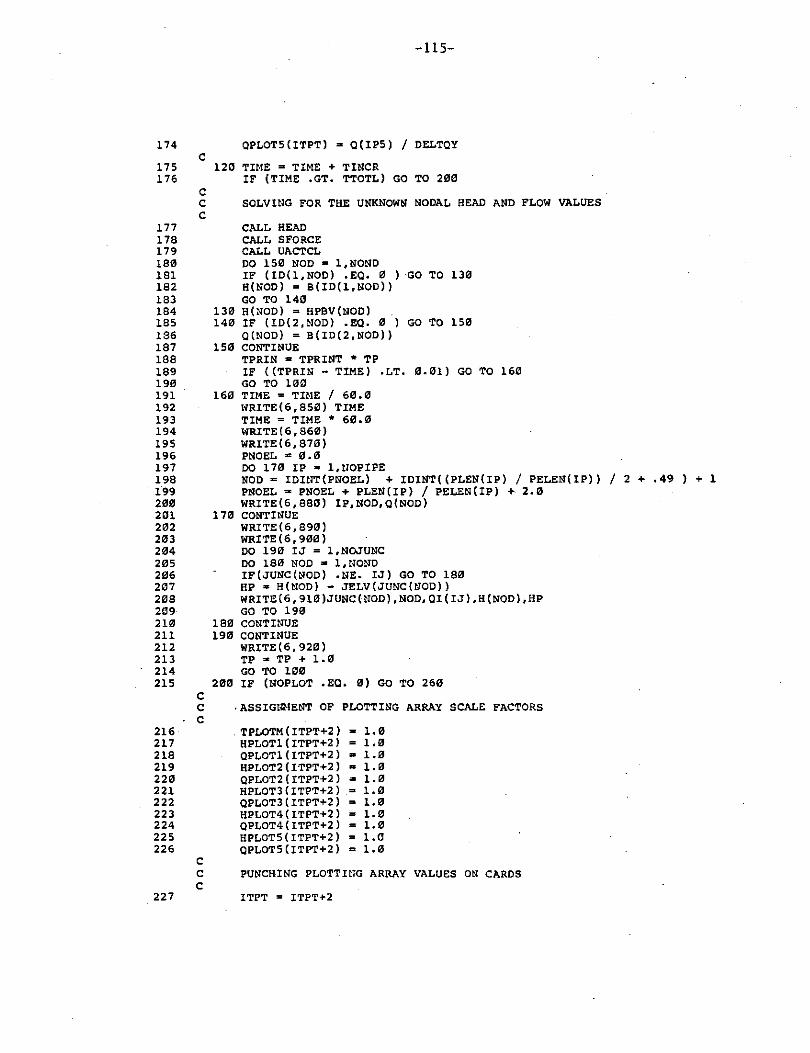
-llS-
174 QPLOTS{ITPT) = Q{IPS) / D<QY c
175 120 TIME = TIME + TINCR 176 IF {TIME .GT. TTOTL) GO TO 200
c C SOLVIllG FOR TKE UNKNOWN NODAL HEAD AND FLOW VALUES c
177 CALL HEAD 178 CALL SFORCE 179 CALL UACTCL 180 DO 150 NOD• l,NOND 181 IF {ID{l,NOD) .EQ. 0 ) ·GO TO 130 182 H{NOD) = B{ID(l,NOD)) 183 GO TO 140 184 130 H{NOD) = HPBV{NOD) 185 140 IF (ID{2,NOD) .EQ. 0) GO TO 150 186 Q(NOD) = B{ID(2,NOD)) 187 150 CONTINUE 188 TPRIN • TPRINT * TP 189 IF {(TPRIN - TIME) .LT. 0.01) GO TO 160 190 GO TO 100 191 160 TIME= TIME/ 60.0 192 WRITE{6,85a) TIME 193 TIME= TIME* 60.0 194 WRITE(6,860) 195 WRITE(6,870) 196 PNOEL • 0.0 197 DO 170 IP• l,tlOPIPE 198 NOD = IDUIT{PNOEL) + IDINT{ {PLEN{IP) / PELEN{IP)) / 2 + • 49 ) + l 199 PNOEL = PNOEL + PLEN{IP) / PELEN(IP) + 2.0 200 WRITE{6,880) IP,NOD,Q{NOD) 201 170 CONTINUE 202 WRITE{6,890) 203 WRITE{6,900) 204 DO 190 IJ = l,NOJUNC 205 DO 180 NOD• l,N'OND 206 IF(JUNC{NOD) .NE. IJ) GO TO 180 207 HP • H{!IOD) - JELV{JUNC{tWD)) 208 WRITE(6, 910 )JUNC (NOD), NOD, QI ( IJ), H {NOD) ,HP 209 GO TO 190 210 180 CONTINUE 211 190 CONTINUE 212 WRITE(6,920) 213 TP • TP + 1,0 214 GO TO 100 215 200 IF (NOPLOT .EQ. 0) GO TO 260
216 217 218 219 220 221 222 223 224 225 226
227
c C ,ASSIGllMENT OF PLOTTING ARRAY SCALE FACTORS c
c
. TPLOTM ( ITPT+2) HPLOTl(ITPT+2) QPLOTl( ITPT+2) HPLOT2 ( I TPT+ 2 ) QPLOT2(ITPT+2) HPLOT3(ITPT+2) QPLOT3(ITPT+2) HPLOT4(ITPT+2) QPLOT4(ITPT+2) HPLOTS ( ITPT+2) QPLOT5(ITPT+2)
"" l. 0 1.0
=- 1.0 • 1.0 a 1.0 = 1.0 =- 1.0 = 1.0
1.0 =- 1.0 = 1.0
C PUNCHING PLOTTING ARRAY VALUES ON CARDS c
ITPT = ITPT+2
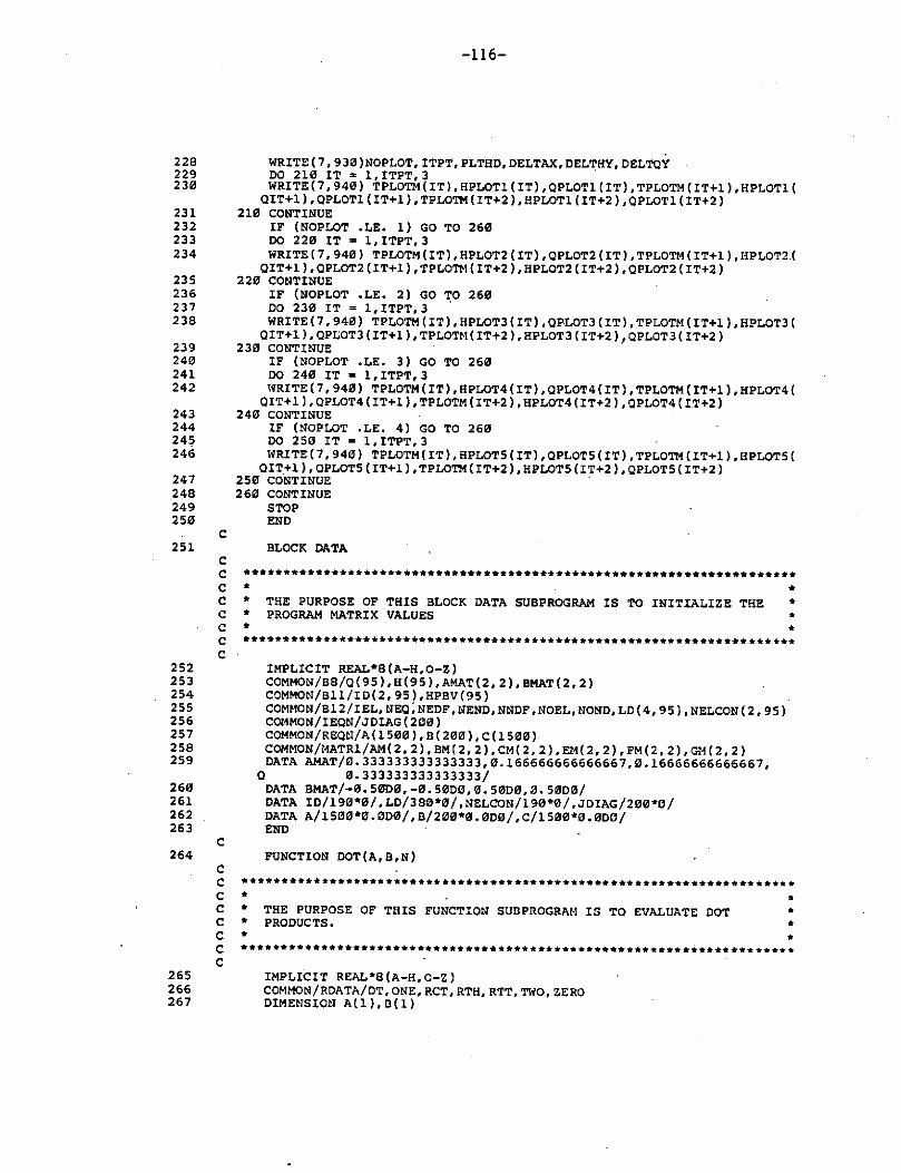
228 229 230
231 232 233 234
235 236 237 238
239 240 241 242
243 244 245 246
247 248 249 2511
c 251
c c c c c c c c
252 253 254 255 256 257 258 259
260 261 262 263
c 264
c c c c c c c c
265 266 267
-116-
WRITE(7,930)NOPLOT,ITPT,PLTHO,DELTAX,OELTHY,OELTQY DO 210 IT = l, ITPT, 3 . WRITE(7,940) TPLOTM(IT),HPLOTl(IT),QPLOTl(IT),TPLOTM(IT+l),HPLOTl(
QIT+l),QPLOTl(IT+l),TPLOTM(IT+2),HPLOTl(IT+2),QPLOTl(IT+2) 210 CONTINUE
IF (NOPLOT .LE, l} GO TO 260 DO 220 IT= l,ITPT,3 WRITE ( 7, 940) TPLOTM( IT), HPLOT2 (IT), QPLOT2 (IT), TPLOTM ( IT+l), HPLOT2.(
QIT+l), QPLOT2 (IT+l), TPLOTM ( IT+2), HPLOT2 ( IT+2}, QPLOT2 ( IT+2) 220 CO!ITINUE
IF (NOPLOT ,LE. 2) GO TO 2611 00 2311 IT= l,ITPT,3 . WRITE ( 7, 9411) TPLOTM (IT), HPLOT3 (IT), QPLOT3 (IT), TPLOTM ( IT+l). HPLOT3 (
QIT+l), QPLOT3 (IT+l), TPLOTM ( IT+2), HPLOT3 ( IT+2) 1 QPLOT3 ( IT+2) 2311 CONTINUE
IF (NOPLOT ,LE, 3) GO TO 260 DO 240 IT= l,ITPT,3 WRITE ( 7, 940) TPLOTM (IT), HPLOT4 (IT), QPLOT4( IT}, TPLOTM ( IT+l), HPLOT4 (
QIT+l}, QPLOT4 ( IT+l), TPLOTM ( IT+2), HPLOT4( IT+2), QPLOT4 ( IT+2) 240 CONTINUE
IF (NOPLOT ,LE, 4) GO TO 2611 DO 250 IT• l,ITPT,3 WRITE(7,940} TPLOTM(IT),HPLOT5(IT},QPLOT5(IT),TPLOTM(IT+l),HPLOT5(
QIT+l),QPLOT5(IT+l),TPLOTM(IT+2),HPLOT5(IT+2),QPLOT5(IT+2) 250 CONTINUE . 2 60 CONTINUE
STOP ENO
BLOCK DATA
••••••••••••••••••••••••••••••••••••••••••••••••••••••••••••••••••••• • * THE PURPOSE OF THIS BLOCK DATA SUBPROGRAM IS TO INITIALIZE THE * PROGRAM MATRIX VALUES •
• • • • •••••••••••••••••••••••••••••••••••••••••••••••••••••••••••••••••••••
IMPLICIT REAL*8(A-H,O-Z) COMMON/B8/Q(95},H(95),AMAT(2,2),BMAT(2,2) COMMON/Bll/ID( 2, 95), HPBV(95) COMMON/Bl2/IEL,NEQ;NEDF,NENO,NNDF,NOEL,tlONO,LD(4,95),NELCON(2,95) COHMON/IEQN/JDIAG(200) COMMON/REQtl/A( l 500), B( 200}, C( l 500) COMMON/MATRl/AM(2, 2), BM( 2, 2) ,CM( 2, 2) ,EM(2, 2), FM(2, 2), GM(2, 2) DATA AMAT/0.333333333333333,0,166666666666667,0.16666666666667,
Q 0.333333333333333/ DATA BMAT/-0.5000,-0.50D0,0.5000,0,50D0/ DATA ID/190*0/,LD/380*0/,NELCON/190*0/,JDIAG/200*0/ DATA A/1530*0.0D0/,B/200*0,0D0/,C/l500*0.0D0/ END
FUNCTION DOT(A,B,N}
••••••••••••••••••••••••••••••••••••••••••••••••••••••••••••••••••••• • • * THE PURPOSE OF THIS FUNCTION SUDPROGRAM IS TO EVALUATE DOT * * PRODUCTS. * • • *********************************************************************
IMPLICIT REAL*8(A-H,O-Z) COMMON/RDATA/DT,ONE,RCT,RTH,RTT,TWO,ZERO DIMENSION A(l),B(l)
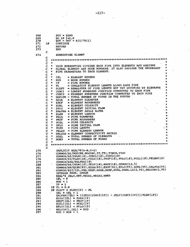
268 269 270 271 10 272 273
c 274
c c c c c c c c c c c c c c c c c c c c c c c c c c c c c c c c c
275 276 277 278 279 280 281 282 283 284 285 286 287 288 289 290 291 292 293 294 295 296 297
DOT =- ZERO DO 10' I•l,tt DOT= DOT+ A(I)*B(I) CONTHlUE RETURN END
SUBROUTINE ELEM!IT
-117-
********************************************************************* • * THIS SUBROUTINE DIVIDES EACH PIPE INTO ELEMENTS AND ASSIGNS * GLOBAL ELEMWT AND NODE NUMBERS. IT ALSO ASSIGNS THE NECESSARY * PIPE PARAMETERS TO EACH ELEMENT. • • • • • • • • • • • • • • • • • • • • • • • • •
IEL NOD IP PL PLEFT JUNCl JUNC2 NOP I PE EDIA ERUF ECEL EFLO EALPHA ELEN PDIA PRUF PCEL PFLO PLEN PE LEN NELCON NOEL NOND
• ELEMENT NUMBER = NODE NUMBER = PIPE NUMBER =- CUMLATIVE ELEMENT LENGTH ALONG EACH PIPE
REMAitlDER OF PIPE LENGTH NOT YET OCCUPIED BY Etn,.lENTS • LOWEST NUMBERED JUtlCTION CONNECTED TO EACH PIPE • HIGHEST NUMBERED JUNCTION CONNECTED TO EACH PIPE
TOTAL NUMBER OF PIPES IN THE SYSTEM • ELEMENT OIAt1ETER • ELEMENT ROUGHNESS • ELEMENT CELERITY • ELEMENT UIITIAL FLOW • ELEMENT ANGLE ALPHA • ELEMENT LENGTH • PIPE DIAMETER • PIPE ROUGHNESS • PIPE CELERITY • PIPE INITIAL FLOW • PIPE LENGTH • PIPE ELEMEtlT LENGTH • ELEMENT CONNECTIVITY MATRIX • TOTAL NUMBER OF ELEMENTS • TOTAL NUMBER OF NODES
• • • • • • • • • • • • • • • • • • • • • • • • • • • • •
••••••••••••••••••••••••••••••••••••••••••••••••••••••••••••••••••••• IMPLICIT REAL*8(A-H,O-Z) COMMOtl/Bl/NOPIPE, NOJUNC, TT, TTl, TINCR, VISC COMMON/B2/PNUM ( 10), JUNCl ( 10), JUNC2 ( 10) COt1MON/B3/PLEN( 10), PDIA ( 10), PRUF (l!l), PFLO( 10), PCEL( 10), PELEN( 10) COMMON/B3A/PALPIIA( 10) COMMON/B4/JNUM ( 10), JELV (10), NOCP ( 10), CPMUM (HJ, 5) COMMON/B9/ELEN(95), EDIA( 95), ERUF (95), EFL0(9 5), ECEL (95), EALPHA( 95) COMMON/Bl2/I.E:L,NEQ,NEDF,NEND,NNDF,NOEL,NOND,LD(4,95),NELCON(2,95) INTEGER PNUM, CPNUM REAL*8 JELV, MHT, MDIAl, MDIA2, MHED IEL = 0 NOD 2 1 IP= l
10 PL= 0.0 20 PLEFT = PLEN(IP) - PL
IEL = IEL + l EALPHA(IEL) ~ ((JELV(JUtlC2(IP)) - JELV(JU~Cl(IP)))/PLEN(IP)) EDIA(IEL) PDIA(IP) ERUF(IEL) • PRUF(IP) ECEL(IEL) = PCEL(IP) EFLO(IEL) = PFLO(IP) NELCON ( l, IEL) = NOD HOD= NOD+ l
298 299 300 301 302 303 304 305 306 307 308 309 310 311 312 313
c 314
c c c c c c c c c c c c c c c c c c c c c c c c c c
315 316 317 318 319 320 321 322 323 324 325 326 327 328 329 330 331 332 333 334
-118-
NELCON(2,IEL) = NOD IF (IDINT(PLEFT).LE.PELEN(IP)) GO TO 30 ELEN(IEL) • PELEN(IP) PL • PL + PELEN(IP) GO TO 20
30 ELEN(IEL) • PLEFT PALPHA(IP) • EALPHA(IEL) IF (IP ,EQ. NOPIPE) GO TO 40 IP= IP+ l NOD = NOD + l GO TO 10
40 CONTINUE NONO = NOD NOEL= IEL RETURtl END
SUBROUTINE JUNCTN
••••••••••••••••••••••••••••••••••••••••••••••••••••••••••••••••••••• • • • • • • • • • • • • • • • • • • • • • •
THIS SUBROUTINE IDENTIFIES THE CONIIECTil!G ELEMENT NODES AT EACH PIPE JUNCTION ANO IDENTIFIES THE NODE NUMBERS IN WHICH HEAD VALUES ARE PRESCRIBED,
IEL IJ IP NOD PL JUNC NPIPE PLEFT JNOD IO
NONO NOCP NOP I PE PLEN PE LEN
• ELEMENT NUMBER • JUHCTION NUMBER = PIPE NUMBER • NODE NUMBER • CUMLATIVE NODE LENGTH ALONG EACH PIPE • JUNCTION NUMBER CONNECTED TO EACH NODE (OR ZERO) • PIPE NUMBER CORRESPONDING TO EACH NODE • REMAINDER OF PIPE LENGTH NOT YET OCCUPIED BY NODES • NOOE !!UMBERS CONNECTED TO EACH JUNCTION • ARRAY TO IDENTIFY PRESCRIBED NODAL VALUES OF HEAD
( l = PRESCRIBED, 0 • FREE J .,. NUl·lBER OF NODES • NUMBER OF CONNECTING PIPES TO EACH JUNCTION = NUMBER OF PIPES IN THE SYSTEM • PIPE LENGTH = PI PE ELEMENT LENGTH
• • • • • • • • • • • • • • • • • * * • • * •••••••••••••••••••••••••••••••••••••••••••••••••••••••••••••••••••••
IMPLICIT REAL*B(A-H,0-Z) COMMON/Bl/NOPIPE,NOJUNC,TT,TTl,TINCR,VISC COMMON/B2/PtlUM ( 10), JUNCl ( l0), JUNC2 (HI) COMMON/83/PLEN( 10), PDIA ( Ul), PROF (HI), PFLO ( 10), PCEL (10), PELEN(lC) COMMON/B3A/PALPHA(l0) COMMON/B4/JNUM ( 10) ,JELV (10) ,NOCP (1"), CPNUM ( 10, 5) COMMON/B7 /JNOD( 10, 5), NPIPE ( 95), JUNC (95) COMMON/Bll/ID(2,95),HPBV(95) COMMON/Bl2/IEL, NEQ, NEDF ,NEND, tlNDF, NOEL, NONO, LD( 4, 95), tlELCON(2, 95) INTEGER PtlUM,CPNUM REAL*B JELV,MiiT,MDIAl,MOIA2,MHED IP• l -IEL = l NOD • 1
10 PL= PELEN(IP) JUNC(NOD) = JUNCl(IP) NPIPE(NOD) • IP IF (PELEN(IP) .GE, PLEN(IPl) GO TO 30
20 NOD =- NOD + l JUNC (NOD) = 0

335 336 337 338 339 340 341 342 343 344 345 346 347 348 349 350 351 352 353 354 355 356 357 358 359 360 361 362 363 364 365
c 366
c c c c c c c c c c c c c c c c c c c c c c
367 368 369 370 371 372 373 374 375
PLEFT • PLEtl(IP) - PL NPIPE(NOD) = IP PL= PL+ PELEN(IP)
-119-
IF (IDINT(PLEFT) ,LE, PELEt<(IP)) GO TO 311 GO TO 2\l
30 NOD s NOD+ l JUNC(NOD) • JUNC2(IP) NPIPE(NOD) = IP IF (IP ,EQ, NOPIPE) GO TO 4\l IP= IP+ 1 NOD= NOD+ l IEL = IEL + l GO TO lll
40 DO 60 IJ ~ l,NOJUNC IP = l NOD = 1
50 IF (JUNC(NOD) ,EQ. IJ) GO TO 55 NOD = tJOD + l GO TO 50
55 JNOD(IJ,IP) NOD IF (IP ,EO, NOCP(IJ)) GO TO 60 IP,. IP+ l NOD= NOD+ l GO TO 50
60 CONTINUE DO 100 N • l,NOND IF (JutlC(N) ,EQ, 0) GO TO 100 ID(l,N) = 1
101' CONTINUE RETURN END
SUBROUTINE NODE
••••••••••••••••••••••••••••••••••••••••••••••••••••••••••••••••••••• • • * THIS SUBROUTINE ASSIGNS INITIAL FLOWS AND HEADS TO EACH NODE, • • • * IEL • ELEMENT NUMBER • • IP • PIPE NUMBER * • NOD • NODE NUMBER • * PL = CUMULATIVE NODE LENGTH ALONG EACII PIPE • • PLEFT = REMAitlDER OF PIPE LENGTH NOT YET OCCUPIED BY NODES • • JUNClS = LOWEST NUMBERED JUNCTION CONNECTED TO EACH PIPE • • JUNC2S • HIGHEST NUMBERED JUNCTION CONNECTED TO EACH PIPE • * NOP I PE = NUMBER OF PIPES IN THE SYSTEII * * MHED • MANHOLE INITIAL HEAD * * PLEN = PIPE LENGTH * * . PELEN s: PIPE ELEMENTLS:NGTH * * PFLO • PIPE INITIAL FLOW * * H • KNOltN NODAL HEAD VALUE • • 0 = KNOWN NODAL FLOW VALUE • • • •••••••••••••••••••••••••••••••••••••••••••••••••••••••••••••••••••••
IMPLICIT REAL*8(A-H,O-Z) COMMON/Bl/NOPIPE,NOJUNC,TT,TTl,TINCR,VISC COMMON/B2/Pt1UM ( 10), JUNCl ( 10), JUNC2 ( 10) COMMON/B3/PLEN(l0),PDIA(l0),PRUF(l0),PFLO(l0),PCEL(l0),PELEN(l0) COMMON/B3A/PALPHA(l0) COMMON/84/JNUM ( 10), JELV ( 10), NOCP ( 10), CPtlUM ( 10, 5.) COMMON/BS/KEY( 10), MHT(Hl), MDIAl (10), MDIA2 ( 10), MHED(lO) COMMOtl/88/0(95), H (95) ,AMAT (2, 2), BMAT(2, 2) COMMO>l/39 /ELEiH 95), EDIA ( 95), ERUF ( 9 5), EFLO ( 95), ECEL ( 95), EAL PP.A( 95)
376 377 378 379 380 381 382 383 384 385 386 387 388 389 390 391
392 393 394 395 396 397 398 399 400 401 402 403 404
c 405
c c c c c c c c c c c c c
406 407 408 409
c c c
410 411 412 413 414 415 10 416 417 418 20 419 30 420 40
c
-120-
UITEGER PNUM, CPNUM REAL*S JELV,MHT,MDIAl,tIDIA2,MHEO IP• l IEL • 1 NOD • l
10 PL• 0.0 JUNClS • JUNCl(lP) JUNC2S • JUNC2(1P) H(NOO) • MHEO(JUNClS) O(NOO) • PFLO(lP)
20 PLEFT • PLEN(lP) - PL PL= PL+ PELEN(IP) IF (lOINT(PLEFT).LE.PELEN(IP)) GO TO 30 IEL a IEL + l NOD a NOD+ 1
'H(NOO) • MHEO(JUNClS) +PL* (MHEO(JUNC2S) - MHEO(JUNClS)) / C PLEN(IP)
O(NOO) • PFLO(IP) GO TO 20
30 NOD :a NOD+ l H(NOO) • MHEO(JUNC2S) O(NOO) • PFLO(IP) IF (IP .EQ. NOPIPE) GO TO 40 IP = IP + 1 IEL •!EL+ l NOD=NOO+l GO TO 10
40 CONTINUE RETUR."I -ENO
SUBROUTINE PROFIL
********************************************************************* * * * THE PURPOSE OF THIS SUB·ROUTINE IS TO CALCULATE THE NUMBER OF * * EQUATIONS ANO ESTABLISH THE DIAGONAL ENTRY ADDRESSES. * * * * NEO • NUMBER OF EQUATIONS * * JOIAG s DIAGOtiAL ARGUMENT NUMBERS OF COEFFICIEtlT MATRIX * * NOEL • NUMBER OF ELEMENTS * * NONO • NUMBER OF NODES * * * ·········································~···························
IMPLICIT REAL•8(A-H,O-Z) COl1MON/Bll/IO( 2, 95), HPBV( 95) COMMON/Bl2/IEL,NEQ,NEOF,NEHO,NNDF,NOEL,NOUO,LD(4,95),NELCON(2,95) COMMON/IEQN/JOIAG ( 200)
SET UP THE EQUATION NUMBERS.
NEQ a 0 DO 43 !I= l,NO!ID DO 30 I::::i:l, t1NDF J • IO(I,tl) IF (J) 30,la,20 NEO•NEO+l IO(I,N) • NEQ GO TO 30 ID(I,tl) = 0 CONTUIUE CO:ITINUE
421 422 423 424 425 426 427 428 429 430 431 432 433 434 435 436 437 438
439 440 441 442 443 444 445
c c
50 60 70 80 90 c c c
100
c
-121-
COMPUTE THE COLUMN HEIGHTS.
00 90 N::::111, NOEL DO 80 I=l, NEND II = NELCON(I,N) DO 70 K•l, NNOF KK = ID (K, 11) IF (KK .LE. 0) GO TO 70 DO 60 J=I, NEND JJ = NELCON(J,N) DO 50 L=l,NNDF LL = ID(L,JJ) IF (LL .LE. 0) GO TO 50 Mu MAX0(KK,LL) JDIAG(M) = MAX0(JDIAG(M),IABS(KK-LL)) CONTHIOE CONTINUE cot,TINUE CONTINUE CONTINUE
COMPUTE THE DIAGONAL ADDRESSES WITHIN THE PROFILE.
JDIAG(l) • l IF (NEQ .EQ. 1) RETURN DO 100 N•2,NEQ JDIAG(N) = JDIAG(N) + JDIAG(N-1) + l CONTINUE RETURN END
446 SUBROUTINE ELEQN
447 448 449
450
451 452 453 454 455 456 457 458
c c ••••••••••••••••••••••••••••••••••••••••••••••••••••••••••••••••••••• c c c c c c c c c c
• • • * * * * * * •
THE PURPOSE OF THIS SUBROUTINE EQUATION NUMBER ARRAY.
!EL = ELEMENT NUMBER NOD = NODE NUMBER NOEL = NUMBER OF ELEMENTS NONO = NUMBER OF NODES NELCOll = ELEME~'T CONNECTIVITY
• IS TO GENERATE THE ELEMENT •
* • • • • *
MATRIX • * c •••••••••••••••••••••••••••••••••••••••••••••••••••••••••••••••••••••
c
c c c
c c c
10 20
IMPLICIT REAL*8(A-H,O-Z) COMMON/Bll/lD(2,95),HPBV(95) COMMON/Bl2/IEL, m:Q, NEDF, NENO, NNDF, NOEL, NONO, LO( 4, 95), NELCON( 2, 95)
LOOPING OVER THE ELEMENTS.
DO 30 IEL=l,NOEL
DETERMINING THE ELEMENT EQUATION NUMBER ARRAY.
DO 20 NOO=l,NEND IC= (NOD - 1)*2 NODE• NELCON(NOD,IEL) DO 10 J•l, 2 !DC = ID(J ,NODE) IF (!DC .GT. 0) LD(J+IC,IEL) !DC CONTINUE CONTl!lUE
459 30 460 461
c 462
c c c c c c c c c c c c c c· c c c
463 464 465 466
c c c
467 468 469 470 471 472 473 474 475 476 477 478 479 480 481 482 483 484
c 485
c c c c c c c c c c c c c c c
CONTINUE RETURN END
SUBROUTINE ESTIFF
· -122-
********************************************************************* * * THIS SUBROUTINE GENERATES THE ELEMENT STIFFNESS MATRIX • * STIFF * TT * TTl • AM * BM * CM * EM * FM * GM •
• STIFFNESS COEFICIENT MATRIX • TINCR * THETA . • TINCR * (1.0 - THETA)
."A" MATRIX (SEE GOVERNitlG EQUATIONS.) "B" MATRIX (SEE GOVERNING EQUATIONS)
• "C(O)" MATRIX (SEE GOVERNING EQUATIONS) • "E" MATRIX (SEE GOVERNING EQUATIONS) • "F" MATRIX (SEE GOVERNING EQUATIONS) • "G" MATRIX (SEE GOVERNING EQUATIONS)
• • • • • • • • • • • • • •••••••••••••••••••••••••••••••••••••••••••••••••••••••••••••••••••••
IMPLICIT REAL*8(A-H,0-Z) COMMON/Bl /NOP I PE, NOJUNC, TT, TT!, TINCR, VISC COMMON/WORK/STIFF(4,4),FORCE(4) COMMON/MATR1/AM(2, 2), BM(2, 2) ,CM(2, 2) ,EM(2, 2), FM(2, 2) ,GM(2, 2)
ASSIGNMENT OF ELEMENT STIFFNESS MATRIX VALUES
STIFF(l,1) • EM(l,l) STIFF(l, 2) TT* (FM(l,l) + GM(l, l)) STIFF(l,3) • EM(l,2) STIFF(l,4) • TT* (FM(l,2) + GM(l, 2)) STIFF(2,l) • TT* BM(l,1) STIFF(2,2) AM(l,l) +TT* CM(l,l) STIFF(2,3) •TT* BM(l,2) STIFF(2,4) • AM(l,2) + TT * CM(l, 2) STIFF(3,l) • EM(2,l) STIFF(3,2) = TT* (FM(2,l) + GM(2,l)) STIFF(3,3) -EM(2,2) STIFF(J, 4) • TT * (FM(2,2) + GM(2,2)) STIFF(4,l) -TT* BM(2,1) STIFF(4,2) • AM(2, l) + TT * CM(2,l) STIFF(4,3) • TT* BM(2,2) STIFF(4,4) •AM(2,2) +TT * CM(2,2) RETURN END
SUBROUTINE HEAD
··························································~·········· • • * THIS SUBROUTINE Cl\LCULATES THE '10DAL HEAD (H (N+l)) VALUES AT * * EACH MANHOLE TO BE USED AS PRESCRIBED BOUNDARY VALUES (HPBV) * * BEFORE EACH GENERAL SYSTEM SOLUTION. * • • • • • • • •
NOCP JNOD NPIPE OJ 0 TIME TINCR
• NUMBER OF CONNECTING NODES FOR EACH JUNCTION • NODE NUMBERS CONNECTED TO EACH JUNCTION • PIPE NUMBER CORRESPOND1'1G TO EACH l!EAD • FLOl'I INTO JUNCTION FROM A NODE • KNO\IN NODAL FLOW VALUE ,. TIME SINCE SIMULATIOU STARTED "" TIME INCRE.."'1:ENT
* * • • • • • •
-123-
• QIN • HYDROGRAPR INITIAL FLOW • • QPK = HYDROGRAPH PEAK FLOW • • TPK .a HYDROGRAPH TIME TO PEAK • • TBAS =- HYDROGRAPH TIME BASE • • QI • MANHOLE INFLOW • • QSUM -SUM OF FLOWS INTO JUNCTION • • TQSUM • VOLUME OF WATER INTO JutlCTION • • AMl =- MANHOLE AREA • • AM2 =-OVERFLOW STORA.GE AREA • • VM = MANHOLE VOLUME CAPACITY • • WHTl • WATER HEIGHT AT JutlCTIOtt FROM PREVIOUS TIME STEP • • WHT • WATER HEIGHT ABOVE MANHOLE !"ROM PREVIOUS TIHE STEP • • WHT2 • WATER HEIGHT AT JUtlCTION FOR PRESENT TIME STEP • • HPBV • HEAD PRESCRIBED BOUNDARY VALUE (JUNCTION HEAD FOR • • PRESENT TIME STEP) • • •
c c c c c c c c c c c c c c c c c c
*********************************************************************
486 487 488 489 490 491 492 493 494 495 496 497 498 499 500 501 502
503 504 505 506 507 508 509 510 511 512 513
c c c
c c c
IMPLICIT REAL*S(A-H,0-Z) DIMENSION QJ(95) COl-.1MON/Bl/NOPIPE, NOJUNC, TT, TTl, TINCR, VISC COMMON/B2/PNUM(l0),JUNCl(l0),JUNC2(10) COMMON/B4/JNUM ( 10), JELV ( 10) ,NOCP ( 10), CP!l!JM ( 10, 5) COMMON/B5/KEY(l0),MIIT(l0),MDIAl(lg),MDIA2(10),MIIED(l0) COMMON/B6/QI(10),QIN(l0),QPK(10),TPK(10),TBAS(10),TIME COMMON/B7/JNOD(l0,5),NPIPE(95),JUNC(95) COMMON/B8/Q(95),H(95),AMAT(2,2),BMAT(2,2) COMMON/B9/ELEtl(95), EDIA( 95), ERUF (95), EFLO ( 95), ECEL( 95), EALPHA( 95) COMMON/Bll/ID(2,95),HPBV(95) COMMON/Bl2/IEL,NEQ,NEDF,NEND,NNDF,NOEL,NOND,LD(4,95),NELCON(2,95) INTEGER PNUM, CPNUM REAL*S JELV,MHT,MDIA1,MDIA2,MHEO PI• 3,14159265358979300 DO 13 NOD• l,NOND
10 HPBV(NOD) • 0,0
20 30
GEOMETRY CALCULATION FOR THE PIPES CONNECTING EACH JUNCTION
00 150 IJ = l,NOJUtlC NOCPS = NOCP(IJ) IF (KEY(IJ) ,EQ, 1) GO TO lJlil 00 30 N = l,NOCPS JNODS = JNOD(IJ,N) NPIPES = NPIPE(JNODS) IF (JUNCl(NPIPES) ,EQ, IJ) GO TO 20 QJ(JNODS) • Q(JNODS) GO TO Jlil QJ(JNODS) • 0,0 - Q(JNODS) CONTitlUE
CALCULATION OF HYDROGRAPH INFLOt;
514 IF (TIME ,GT, TBAS(IJ)) GO TO 50 515 IF (TIME ,GT, TPK(IJ)) GO TO 40 516 QI(IJ) • QIN(IJ) + (TIME - TINCR) * (QPK(IJ) - QIN(IJ)) / TPK(IJ) 517 GO TO 60 518 40 QI(IJ) = QPK(IJ) + ((QIN(IJ) - QPK(IJ)) * (TIME - TINCR - TPK(IJ))
Q / (TBAS(IJ) - TPK(IJ))) 519 GO TO 60 520 50 QI(IJ) = QIN(IJ) 521 60 QSUM • QI(IJ)
c C CALCULATION OF tlPBV AT EACH MANHOLE (JUNCTION CO~ITHIUITY EQUATION) c
-124-
522 DO 7C N = l,NOCPS 523 JNODS = JNOD(IJ,N) 524 70 QSUM = QSUM + QJ(JNODS) 525 TQSUM • QSUM * TINCR 526 AMl •PI* ((MDIAl(IJ) / 12.0) •• 2.0) / 4.0 527 VM = AMl * MHT(IJ) 528 AM2 =PI* ((MDIA2(IJ)) ** 2.0) / 4.0 529 JNODS = JNOD(IJ,l) 53C WHTl • H(JNODS) - JELV(IJ) 531 IF (WHTl .GT. MHT(IJ)) GO TO 90 532 TQSUM = TQSUM + WHTl * 'AIU 533 IF (TQSUM .GT. VM) GO TO 100 534 80 WHT2 = TQSUM / AMl 535 GO TO 110 536 90. WHT = WHTl - MHT( IJ) 537 TQSUM • TQSUM + MHT(IJ) * AMl + WHT * AM2 538 IF (TQSUM' ,LE. VM) GO TO 80 539 100 WHT2 • MHT(IJ) + (TQSUM - VM) / AM2 540 110 DO 120 N = l,tlOCPS 541 JNODS = JNOD(IJ,N) 542 120 HPBV(JNODS) • WHT2 + JELV(IJ) 543 GO TO 150 544 130 QI(IJ) • 0.0 545 DO 140 N • l,NOCPS 546 JNODS = JNOD(IJ,N) 547 140 HPBV(JNODS) = H(JNODS) 548 150 CONTINUE 549 RETURN 550 END
c 551 SUBROUTINE SFORCE
c c c c c c c c c c c c c c c c c c c c c c c c c c c c c c c c c
••••••••••••••••••••••••••••••••••••••••••••••••••••••••••••••••••••• • * THIS SUBROUTINE GENERATES THE ELEMENT FORCE VECTOR
• • • •
• • • • • • • • • • • • • • • • • • • • • • • • • • • •
FORCE AM BM CM EM FM GM Ql Q2 FFl FF2 REl RE2 VISC TTl G ELEN EDIA EAREA ECEL EALPHA ERUF HPBV NELCOtl A B c
= RIGHT HAND SIDE FORCE VECTOR * • "A" MATRIX (SEE GOVERNING EQUATIONS) * = "B" MATRIX (SEE GOVERNUIG EQUATIONS) * • "C(Q)" MATRIX (SEE GOVER.'HNG EQUATIONS) * • "E" MATRIX (SEE GOVERNING EQUATIONS) * • "F" MATRIX (SEE GOVER.~ING EQUATIONS) * • "G" MATRIX (SEE GOVERNING EQUATIONS) * • KNOWU FLOW VALUE AT NODE l * • KNOWN FLOW VALUE AT NOOE 2 * • KNOWN DARCY FRICTION FACTOR AT NODE 1 * • KNOWtl DARcY FRICTION FACTOR AT NODE 2 * • KNOWtl REYNOLDS NUMBER AT NODE. l * • KNOWN REYNOLDS ?WMBER AT NODE 2 * • KINEMATIC VISCOSITY OF FLUID * • TINCR * (1.0 - THETA) * • ACCELERATION DUE TO GRAVITY * • ELEMENT LENGTH * • ELEMENT DIAMETER * • ELEMENT CROSS SECTIONAL AREA * • ELEMENT CELERITY * • ELEMENT ANGLE ALPHA * • ELEMEUT ROUGHNESS * • HEAD PRESCRIBED BOUNDARY VALUE * ""' ELEMENT CONUECTIVTY MATRIX * • GLOBAL COEFFICIENT ARRAY FOR GAUS-CROUT SOLUTION ROUTI~IE* • GLOBAL RHS VECTOR FOR GAUS-CROUT SOLUTION ROUTINE * • GLOBAL C9EFFICIENT ARRAY FOR GAUS-CROUT SOLUTIO~ ROUTINE*
•

-125-
c ••••••••••••••••••••••••••••••••••••••••••••••••••••••••••••••••••••• c
552 IMPLICIT REAL*8(A-H,O-Z) 553 DIMENSION EAREA(95) 554 COMMON/Bl/NOPIPE,NOJUNC,TT,TTl,TINCR,VISC SSS COMMON/B8/Q(95) ,8(95) ,J\MAT(2, 2), BMAT(2, 2) 556 COMMON/B9/ELEN(95),EDIA(95),ERUF(95),EFL0(95),ECEL(95),EALPHA(95) 557 COMMON/Bll/ID(2,95),BPBV(95) 558 COMMON/Bl2/IEL, NEQ, NEDF, NEND, NNDF, NOEL, tlOND, LD(4, 95), NELCON ( 2, 95) 559 COMMON/Bl3/SA,SF,SG 560 COMMON/RLOG/AFAC,AFL,BACK,BFL 561 COMMON/IEON/JDIAG(200), 562 COMMON/REQN/A(l500),B(200),C(l500) 563 COMMON/WORK/STIFF(4,4),FORCE(4) 564 COMMON/MATRl/AM( 2, 2), BM( 2, 2), CM( 2, 2), EM( 2, 2 f. FM( 2, 2), GM (2, 2) 565 LOGICAL AFAC,AFL,BACK,BFL 566 ZERO= 0,000
c C INITIALIZING TBE COEFFICIENT ARRAYS c
567 NAO• JDIAG(NEO) 568 DO 40 !AD= l,NAD 569 A(IAD) • ZERO 570 C(IAD) = ZERO 571 40 CONTINUE
c C INITIALIZING THE GLOBAL RIGHT HAND SIDE VECTOR c
572 DO 50 NN = l,NEO 573 B(NN) = ZERO 574 50 CONTINUE 575 G = 32.17400 576 DO 1000 !EL= l,NOEL 577 EAREA(IEL) = J.14159265358979300 * ((EDIA(IEL)/12.0) **2.0) / 4.3
578 579 580 581 582 583 584 585
586 587 588 589 590
591
592
593
594
c C CALCULATION OF THE STIFFNESS ARRAY COMPONENTS c
c c c
DO 60 I= 1,2 DO 60 J = l, 2 AM(I,J) SA* ELEN(IEL) * AMAT(I,J) BM(I,J) = G * EAREA(IEL) * BMAT(I,J) EM(I,J) = ELEtl(IEL) * AMAT(I,J) FM(I,J) • SF*ELEN(IEL) * EALPHA(IEL) * AMAT(I,J)/EAREA(IEL) GM(I,J) • SG*ECEL(IEL) * ECEL(IEL) * BMAT(I,J) / (G * EAREA(IEL))
60 CONTINUE
UPDATING THE ELEMENT FRICTION LOSS TERM
_Ql = Q(tlELCOtt(l, IEL)) 02 = Q(NELCOt1(2, !EL)) REl = DABS(Ql * (EDIA(IEL) / 12.0) / (EAREA(IEL) * VISC)) RE2 DABS(Q2 * (EDIA(IEL) / 12.0) / (EAREA(IEL) * VISC)) FFl = 0.2500 / ((DLOGl0((ERUF(IEL) / (3.700 * EDIA(IEL) / 12.0) +
Q 5.7400 / REl •• 0.900))) •• 2) FF2 = 0.2500 / ((DLOG10((ERUF(IEL) / (3.700 * EOIA(IEL) / 12.0) +
Q 5.7400 / RE2 •• 0.900))) •• 2) CM(l,l) • ELEN(IEL) * (0.2000 * FFl * DABS(Ql) + 0.0500
Q * FF2 * DABS(Ql) + 0.0500 * FFl * DABS(Q2) + FF2 * Q DABS(Q2) / 30.0) / (2.0 * EAREA(IEL) * EDIA(IEL) / 12.0)
CM(l,2) ELEN(IEL) • (0.0500 *FF!* DABS(Ql) + , Q FF2 * DABS(Ql) / 30.0 + FFl * DA8S(Q2) / 30.0 + 0.0500 • Q FF2 * DA8S(Q2)) / (2.0 • EAREA(IEL) • EOIA(IEL) / 12.0)
CM(2,l) ELEN(IEL) * (0.0500 * FFl * DABS(Ql) + O F~2 * DAllS{Ql) / 30.0 + FFl * DABS(Q2) / 30.0 + 0.0500 *
595
596 c c c
597 598
c c c
599 600
601
602 603
c c c c
604 605 606 607 608 609 610 611 612 613 614 615 616
c 617
c c c c c c c c c c c c c c c c
618 619 620 621 622 623 624
-126-
FF2 • DABS(Q2)) / (2.0 * EAREA(IEL) * EDIA(IEL) / 12.0) • ELEN(IEL) * (FFl * DABS(Ql) / 30.0 + 0.0500
0 CM(2,2)
0 * FF2 * DABS(Ql) + 0.0500 * FFl * DABS(Q2) + 0.200 * FF2 * DABS(02)) / (2.0 * EAREA(IEL) * EDIA(IEL) / 12.0)
DO 110 NOD• 1,2 0
INITIALIZING THE FORCE VECTOR
FORCE(2 * NOD - l) = ZERO FORCE(2 *NOD)• ZERO
CALCULATION OF ELEMENT RIGHT HAND SIDE VECTOR (FORCE VECTOR)
DO 100 IDF = l,NNDF FORCE(2*NOD-l) = FORCE(2*NOD-l) + EM(NOD,IDFi * H(NELCON(IDF,IEL))
0 - TTl * (FM(NOD,IDF) + GM(NOD,IDF)) * O O(NELCON(IDF,IEL))
FORCE(2 *NOD)= FORCE(2 * NOD) - TTl * BM(NOD,IDF) * O H(NELCON(IDF,IEL)) + (AM(NOD,IDF) -Q TTl * CM(NOD,IDF)) * O(NELCON(IDF,IEL))
100 CONTINUE llll CONTINUE
MODIFYING THE ELEMENT RIGHT HAND SIDE VECTOR TO INCLUDE tlONZERO PRESCRIBED BOUNDARY VALUES.
DO 500 NOD• l,NENO DO 500 IDF • l,. NUDF IF (ID(IDF,llELCON(NOD,IEL)) .GT. 0)GO TO 500 CALL ESTIFF IC• (NOD - l) * NNDF + IDF DO 450 I = l,NEDF FORCE(I) • FORCE(I) - STIFF(I,IC) * HPBV(NELCON(NOD,IEL))
450 CONTINUE 500 CONTilWE
CALL ADDSTF 1000 CONTINUE
RETUR?I END
SUBROUTINE ADDSTF
• *** ········*··············· ................ **** ** ** •••••• *** *** ****** • • • • • • • • • • • •
THE PURPOSE OF THIS SUBROUTIUE IS TO ASSEMBLE THE ELEMENT FORCE VECTOR AND COEFFICIENT MATRIX INTO THE GLOBAL FORCE VECTOR AIID COEFFICIENT MATRIX COIISISTENT WITH THE PROFILE SOLVER •
NEDF IEL A B c
• NUMBER OF ELEMENT DEGREES OF FREEDOM • ELEMENT NUMBER • UPPER PROFILE COEFFICIENT MATRIX ARGUMEIITS • RIGHT HAND SIDE VECTOR ARGUMENTS • LOWER PROFILE COEFFICIENT '1ATRIX ARGUMENTS
• • • • • • • • • • • •
••••••••••••••••••••••••••••••••••••••••••••••••••••••••••••••••••••• IMPLICIT REAL*S(A-ll,0-Z) COMMON/Bl2/IEL,NEQ,NEDF,NEND,NNOF,NOEL,NOND,LD(4,95},NELCON(2,95) COH~ION/RLOG/AFAC,AFL, BACK, BFL COMMON/IEQN/JDIAG(200) COMMON/REQN/A(l500),B(200),C(l500) COMMON/1-IORK/S ( 4, 4), P ( 4) LOGICAL AFAC,AFL,BACK,BFL
625
626 627 628 629 630 631 632
633 634 635 636 637 638
639 640
641
642 643 644 645 646 647 648
649 650 651 652 653 654 655 656 657 658
c
c c c
c 'C c
100 200 c
c
-127-
00 200 J=-1,UEDF
ASSEMBLING THE RIGHT HAND SIDE VECTOR.
K • LD(J,IEL) IF (K .EQ. 0) GO TO 200 IF (BFL) B(K) • B(K) + P(J) IF (.NOT. AFL) GO TO 200 L • JDIAG(K) - K DO 100 I=l,UEDF M = LD(I, IEL)
ASSEMBLING THE UPPER AND LOWER PROFILE COEFFICIENT MATRICES.
IF (M .GT. K .OR. M .EQ. 0) GO TO 100 M = L + M A(M) = A(M) + S(I,J) C(M) = C(M) + S(J,I) CONTINUE COUTINUE
RETURN END
SUBROUTINE UACTCL
********************************************************************* • * TP.B PURPOSES OF THIS SUBROUTINE ARE TO PERFORM FORWARD ELIMI* NATION AND BACKSUBSTITUTION OPERATIONS ON AN UNSYMMETRIC * COEFFICIENT MATRIX WITH A SYMMETRIC PROFILE USING GAUSS-CROUT * ELIMINATION. • • • • • • •
NEQ JDIAG A B c
--= -
NUMBER OF EQUATIONS DIAGONAL ARCiUMENT NfiltBERS OF COEFFICIEt{T MATRIX UPPER PROFILE COEFFICIENT MATRIX ARGU!IENTS RIGHT !iAND SIDE VECTOR ARGUMENTS LOWER PROFILE COEFFICIENT MATRIX ARGUMENTS
• • • • • • • • • • • •
c c c c c c c c c c c c c c c c
•••••••••••••••••••••••••••••••••••••••••••••••••••••••••••••••••••••
c c c c
c
IMPLICIT REAL*B (A-ll, o-z) COMMON/Bl2/IEL,NEQ,NEDF,NEND,NNDF,NOEL,NOND,LD(4,95),NELCON(2,95) COMMON/ROATA/DT,ONE,RCT,RTH,RTT,TWO,ZERO COMMON/RLOG/AFAC,AFL,BACK,BFL COMMON/IEON/JDIAG(200) COMMON/REQN/A(l500),B(200),C(1500) LOGICAL AFAC,AFL,BACK,BFL
FACTOR THE COEFFICIENT MATRIX A INTO UT*D*U AtlD REDUCE THE RIGHT !iAND SIDE VECTOR B.
JR= 0 00 300 J=l,NEO JD = JDIAG (J) JH = JO - JR IF (JH .LE. 1) GO TO 300 IS = J + l - JH IE = J - l IF (.NOT. AFAC) GO TO 250 K = JR + l ID = 0
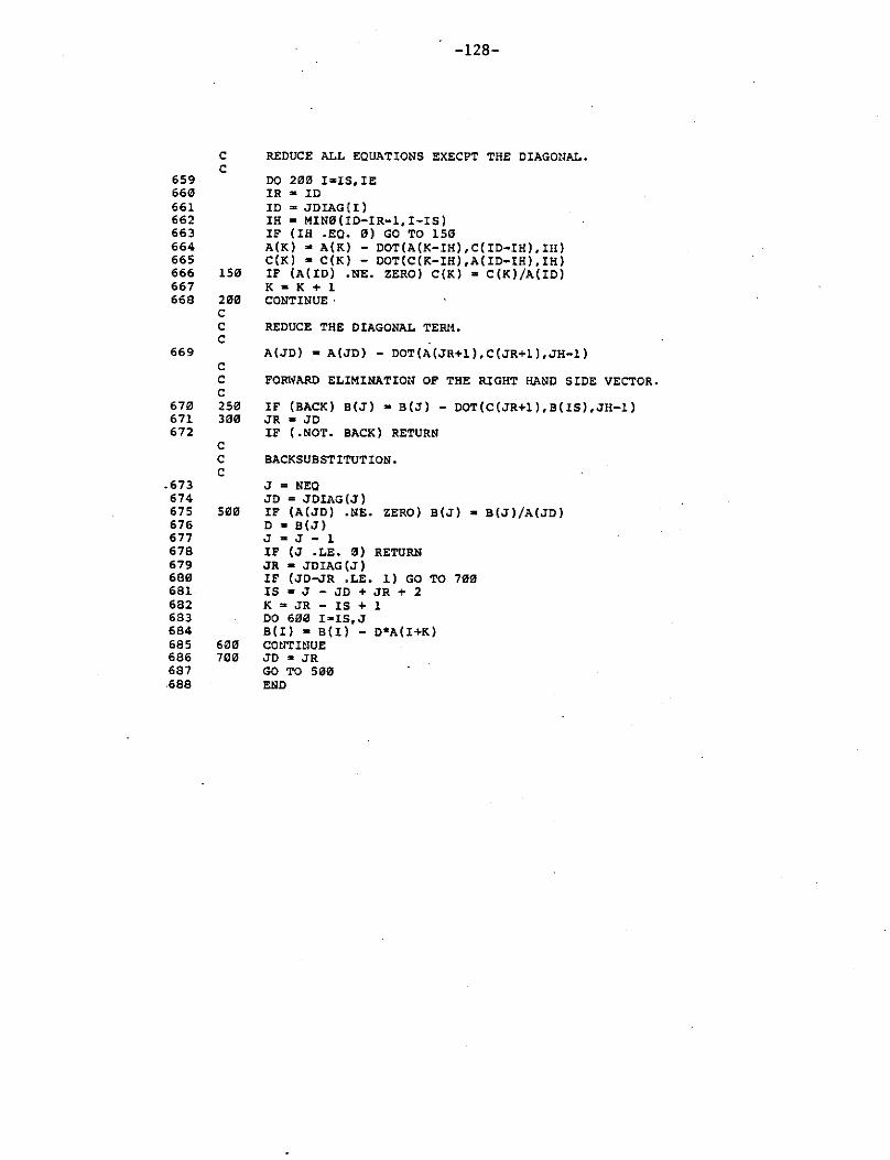
-128-
C REDUCE ALL EQUATIONS EXECPT THE DIAGONAL.
659 660 661 662 663 664 665
c
666 150 667 668 200
c c c
669 c
DO 200 I•IS,IE IR• ID ID = JDIAG(I) IH = MIN0(ID-IR-l,I-IS) IF (IH .EQ. 0) GO TO 1511 A(K) • A(K) - DOT(A(K-IH),C(ID-IH).Ill) C(K) • C(K) - DOT(C(K-IH),A(ID-IH),IH) IF (A(ID) ,NE, ZERO) C(K) • C(K)/A(ID) K • K + l CONTINUE·
REDUCE THE DIAGONAL TERM.
A(JD) • A(JD) - DOT(A(JR+l),C(JR+l),JH-l)
C FORWARD ELIMINATiotl OF THE RIGHT HAND SIDE VECTOR. c
67111 250 IF (BACK) B(J) • B(J) - DOT(C(JR+l).B(IS).J!l-l) 671 300 JR• JD 672 IF (.NOT. BACK) RETURN
c C BACKSUBSTITUTION. c
.673 J = NEQ 674 JD= JDIAG(J) 675 51110 IF (A(JD) .NE. ZERO) B(J) • B(J)/A(JD) 676 D • B(J) 677 J • J - l 678 IF (J .LE. 0) RETURN 679 JR• JDIAG(J) 680 IF (JD-JR .LE. l) GO TO 700 681 IS• J - JD+ JR+ 2 682 K • JR - IS+ l 683 DO 600 I•IS,J 684 B(l) • B(I) - D*A(I+K) 685 6011 COUTHIUE 686 7~0 JD• JR 687 GO TO 500 .688 END
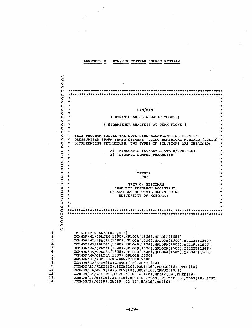
1 2 3 4 5 6 7 8 9
10 11 12 13 14
c c c c c c c c c c c c c c c c c c c c c c c c c c c c c c c c c c c c c c c c
·c c
APPENDIX B DYN/KIN FORTRAN SOURCE PROGRAM
**************************************i~····························· ••••••••••••••••••••••••••••••••••••••••••••••••••••••••••••••••••••• • • • • • • • •
DYN/KIN
( DY?IAMIC AND KINEMATIC MODEL )
STORMSENER AHALYSIS AT PEAK FLOWS
• • • • • • • •
• • • • * THIS PROGRAM SOLVES THE GOVER!IING EQUATIONS FOR FLOW IN * * PRESSURIZED STORM SEWER SYSTEMS USING NUMERICAL FORWARD (EULER) • * DIFFERENCING TECHNIQUES. TWO TYPES OF SOLUTIONS ARE OBTAINED: * • • • • • • • • • • • • • • • • • •
A) KINEMATIC ( STEADY STATE W /STORAGE) B) DYNAMIC LUMPED PARAMETER
THESIS 1982
GREG C. HEITZMAN GRADUATE RESEARCH ASSISTANT
DEPARTMENT OF CIVIL ENGINEERING UNIVERSITY OF KENTUCKY
• • • • • • • • • • • • • • • • •••••••••••••••••••••••••••••••••••••••••••••••••••••••••••••••••••••
•••••••••••••••••••••••••••••••••••••••••••••••••••••••••••••••••••••
IMPLICIT REAL*S(A-H,0-Z) COMMON/Ml/TPLOTM(l500),HPL01A(l500),HPL01B(l500) . COMMON/M2/HPL02A( 1500), HPL02B ( 1500), UPL03A( 1500), HPL038 ( 1500) COMMON/Ml/HPL04A(l500),HPL04D(1500),HPL05A(l500),HPL05B(l500) COMMON/M4/QPL01A(l500),QPL01B(l500),QPL02A(l500),QPL02D(l500) COMMotl/M5/QPL03A( 1500), QPL03B ( 1500), QPL04A( 1500), QPL048 ( 1500) COMMON/M6/QPL05A ( 1500), QPL05B ( 1500) COMMON/Bl/NOPIPE, NOJUNC, TH!CR, VISC COMMON/82/PNUM ( 10), JUNCl ( 10), JUNC2 ( 10) COM!10N/Bl/PLEN( 10), PD!A( 10), PROF ( 10), MLOSS ( 10), PE'LO( 10) COl1MON/B4/JNUM( 10), JELV( 10), ~IOCP (10), CPNUM ( 10, 5) COIIMON/B5/KEY ( 10), MHT ( 10), MDIAl ( 10), MOIA2 ( 10), MHED (la) COMMON/B6/QI (10), Qitl( 10) ,QPK(l0) ,TL.AG( 10) ,TPI<( 10) ,TBAS( 10), TIME COMMON/D8/Q(l0),QA(l0),Q8(10),HA(l0),HD(l0)
-129-
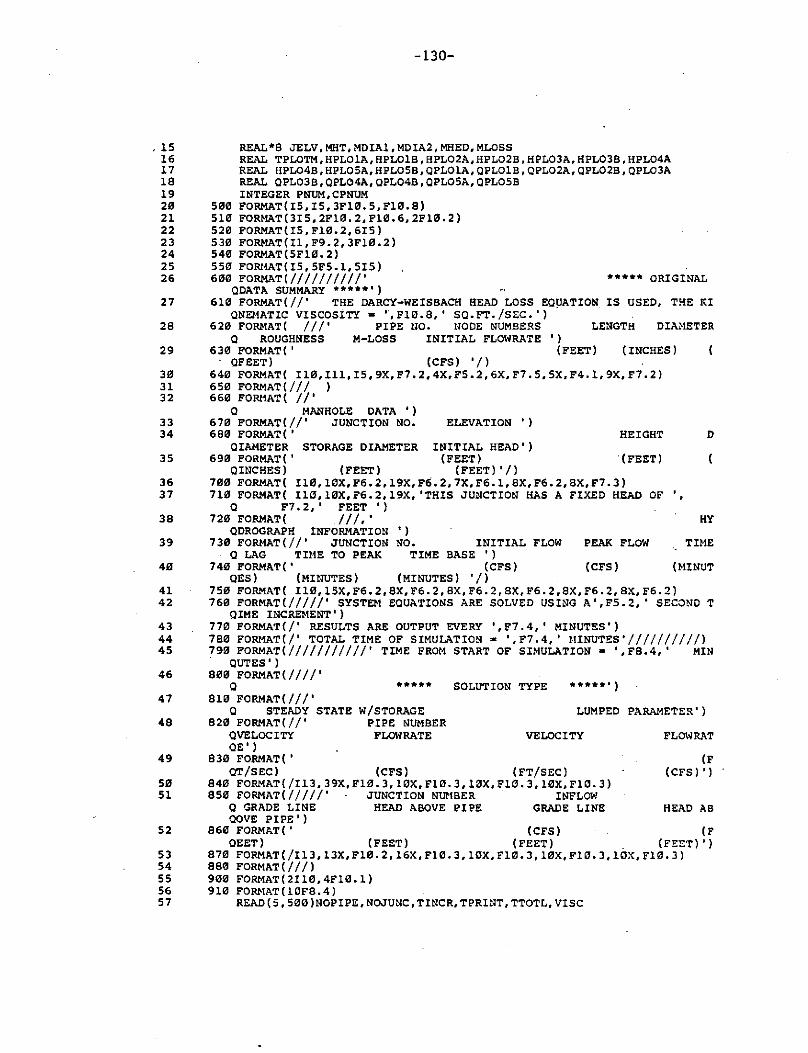
-130-
, 15 REAL*S JELV,MHT,MOIA1,MDIA2,MHED,MLOSS 16 REAL TPLOTM,HPL01A,HPL01B,HPL02A,HPL02B,HPL03A,HPL03B,HPL04A 17 REAL HPL04B,HPL05A,HPLOSB,QPLOlA,OPLOlB,QPL02A,QPL02B,QPL03A 18 REAL QPL03B,QPL04A,QPL04B,QPL05A,QPL05B 19 INTEGER PNUM,CPNUM 20 500 FORMAT(I5,I5,3Fl0.5,Fl0.8) 21 510 FORMAT(3I5,2Fl0,2,Fl0.6,2Fl0.2) 22 520 FORMAT(I5,Fl0.2,6I5) 23 530 FORMAT(Il,F9.2,3Fl0.2) 24 540 FORMAT(5Fl0.2) 25 550 FORMAT(I5,5F5.l,5I5) 26 600 FORMAT(//////////' ***** ORIGINAL
QOATA SUMMARY*****') 27 610 FORMAT(//' THE DARCY-WEISBACH HEAD LOSS EQUATION IS USED, THE KI
QNEMATIC VISCOSiTY = .. ,Fl0.8, 1 SQ.FT./SEC.') . 28 620 FORMAT( ///' PIPE UO. NODE NUMBERS LENGTH DIAMETER
Q ROUGHNESS M-LOSS INITIAL FLOWRATE ') 29 630 FORMAT(' (FEET) (INCHES)
QFEET) (CFS) '/) 30 640 FORMAT( Il0,Ill,I5,9X,F7.2,4X,F5.2,6X,F7.5,5X,F4.l,9X,F7.2) 31 650 FORMAT(/// ) 32 660 FORMAT(//'
Q MANHOLE DATA') 33 670 FORMAT(//' JUNCTION NO. ELEVATION ') 34 680 FORMAT(' HEIGHT D
QIAMETER STORAGE DIAMETER INITIAL HEAD') 35 690 FORMAT(' (FEET) ·(FEET)
CINCHES) (FEET) (FEET)'/) 36 700 FORMAT( Il0,10X,F6.2,19X,F6.2,7X,F6.l,8X,F6.2,BX,F7.J) 37 710 FORMAT( Il0,10X,F6.2,19X, 'THIS JUNCTION HAS A FIXED HEAD OF
O F7.2, 1 FEET') 38 720 FORMAT( ///,' HY
QDROGRAPH INFORMATION') 39 730 FORMAT(//' JUNCTION !10. INITIAL FLOW PEAK FLOW TIME
Q LAG TIME TO PEAK TIME BASE ' ) 40 740 FORMAT(' (CFS) (CFS) (MINUT
QES ) ( MIUUTES) ( MINUTES ) ' /) 41 750 FORMAT( Il0,15X,F6.2,8X,F6.2,8X,F6.2,8X,F6.2,8X,F6.2,8X,F6.2) 42 760 FORMAT(/////' SYSTEM EQUATIONS ARE SOLVED USillG A' ,F5. 2,' SECOND T
QIHE INCREMENT' ) 43 770 FORMAT(/' RESULTS ARE OUTPUT EVERY ',F7,4,' MINUTES') 44 780 FORMAT(/' TOTAL TIME OF SIMULATION • ', F7. 4, ' ?HNUTES' / / ///// / //) 45 790 FORMAT(///////////' TIME FROM START OF SIMULATION• ',FS.4,' MIN
. QUTES') 46 800 FORMAT(////'
0 ***** SOLUTION TYPE *****') 47 810 FORMAT(///'
Q STEADY STATE W/STORAGE LUMPED PARAMETER') 48 820 FORMAT(//' PIPE NUMBER
QVELOCITY FLOWRATE VELOCITY FLOWRAT QE')
49 830 FORMAT( ' (F QT/SEC) (CFS) (FT/SEC) (CFS)')
50 840 FORMAT(/Il3,39X,Fl0.3,10X,Fl0.3,10X,Fl0.3,10X,Fl0.3) 51 850 FORMAT(/////' JUNCTION NU11BER INFLOW
Q GRADE LINE HEAD ABOVE PIPE GRADE LINE HEAD AB QOVE PIPE')
52 860 FORMAT(' (CFS) (F QEET) (FEET) (FEET) (FEET)')
53 870 FORMAT(/Il3,13X,Fl0.2,16X,Fl0.3,10X,Fl0.3,10X,Fl0.3,10X,Fl0.3) 54 880 FORMAT(///) 55 900 FORMAT(2Il0,4Fl0.l) 56 910 FORMAT(lOFB.4) 57 READ(S,500)NOPIPE,NOJUNC,TINCR,TPRINT,TTOTL,VISC
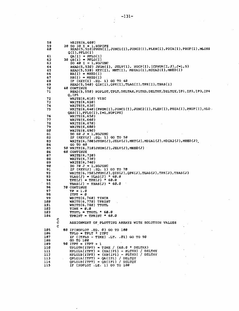
-131-
58 WRITE(6, 600) 59 20 DO 30 I= l,NOPIPE 60 READ( 5, 510 )PNtlf1 (I), JUNCl (I), JUNC2 (I), PLEN( I), PDIA( I). PRUF (I), MLOSS
Q(I), PFLO( I) 61 QA(I) • PFLO(I) 62 30 QB(I) = PFLO(I) 63 DO 40 I= l,NOJUNC 64 READ(5, 520) JNUM(I), JELV(I), tlOCP(I), (CPNUM(I,J),J•l,5) 65 READ(5,530) KEY(I), MHT(I), MDIAl(I),MDIA2(I),MHED(I) 66 HA(I) • MHED(I) 67 HB(I) = MHED(I) 68 IF (KEY(I) .EQ. 1) GO TO 40 69 READ(5, 540) QIN( I) ,QPK(I) ,TLAG,(I) ,TPK( I), TBAS( I) 70 40 CONTINUE 71 READ(S,550) NOPLOT,TPLT,DELTAX,PLTHO,DELTHY',DELTQY,IPl,IP2,IP3,IP4
0,IPS 72 WRITE(6,6l0) VISC 73 WRITE(6,620) 74 WRITE(6,630) 75 WRITE(6, 640) (PNUM(I) ,JUNCl (I ),JUNC2 (I), PLEN( I), PDIA( I), PRUF (I) ,>!LO -
QSS(I),PFLO(I),I•l,NOPIPE) . 76 WRITE(6,650) 77 WRITE(6,660) 78 WRITE(6,670) 79 WRITE(6,6B0) 80 WRITE(6,69C) 81 DO 60 J • l,NOJUNC 82 IF (KEY(J) .EQ. 1) GO TO 50 83 WRITE(6,700)JNUM(J),JELV(J),MHT(J),MDIAl(J),MDIA2(J),MHED(J)_ 84 GO TO 69 85 50 WRITE(6, 7l0)JNUM(J),JELV(J),MHED(J) 86 60 CONTINUE 87 WRITE(6,720) 88 WRITE(6,730) 89 WRITE(6,740) 90 DO 70 J ~ l,30JUNC 91 IF (KEY(J) .EQ. l) GO TO 70 92 WRITE(6, 750)JNUM(J), QIN(J) ,QPK(J) ,TLAG(J) ,TPK(J) ,TBAS(J) 93 TLAG(J) = TLAG(J) * 60,0 94 TPK(J) • TPK(J) * 60.0 95 TBAS(J) = TBAS(J) * 60,0 96 70 CONTINUE 97 TP • 1.0 98 ITPT = 0 99 WRITE(6,760) TINCR
100 WRITE(6, 770) TPRUIT l!ll WRITE(6,780) TTOTL 102 TIME • 0,0 103 TTOTL • TTOTL * 60,0 104 TPRINT • TPRINT * 60.0
c c c
1'15 80 106 107 108 109 90 110 111 112 113 114 115
ASSIGNMENT OF PLOTTING ARRAYS WITH SOLUTION VALUES
IF(NOPLOT ,EQ, 0) GO TO 100 TPLO • TPLT * ITPT IF ( (TPLO - TIME) .LT. ,01) GO TO 90 GO TO 100 ITPT = ITPT + 1 TPLOTM(ITPT) •TIME/ (60,0 * DELTAX) HPLOlA(ITPT) (HA(IPl) - PLTHD) / DELTHY HPLOlB(ITPT) • (HB(IPl) - PLTHD) / DELTHY QPLOlA(ITPT) = QA(IPl) / DELTQY QPLOlB(ITPT) = QB(IPl) / DELTQY IF (NOPLOT ,LE, 1) GO TO 100
-132-
116 HPL02A(ITPT)-= (HA(IP2) - PLTHD) I DELTHY 117 HPL02B(ITPT) = (HB(IP2) - PLTHD) I DELTHY 118 QPL02A(ITPT) • QA(IP2) / DELTQY 119 QPL02B(ITPT) • QB(IP2) / DELTQY 1211 IF (NOPLOT .LE. 2) GO TO 100 121 HPL03A(ITPT) • (HA(IP3) - PLTHD) I DELTHY 122 HPL03B(ITPT) • (HB(IP3) - PLTHD) I DELTl!Y 123 QPL03A(lTPT) • QA(IP3) / DELTQY 124 QPL03B(ITPT) • QB(IP3) / DELTQY 125 IF (NOPLOT .LE. 3) GO TO 100 126 HPL04A(lTPT) = (HA(IP4) - PLTHD) I DELTHY 127 HPL04B(ITPT) • (HB(IP4) - PLTHD) I DELTHY 128 QPL04A(ITPT) = QA(IP4) / DELTQY 129 QPL04B(ITPT) = QB(IP4) / DELTQY 130 IF (NOPLOT .LE, 4) GO TO 100 131 HPL05A(ITPT) = (HA(IP5) - PLTHD) I DELTl!Y 132 HPL05B(ITPT) = (HB(IP5) - PLTHD) I DELTHY 133 QPL05A(ITPT) = QA(IP5) / DELTQY 134 QPL05B(ITPT) • QB(IP5) / DELTQY
c 135 100 TIME ,. TIME + TlNCR 136 IF (TIME ,GT, TTOTL) GO TO 140 137 CALL HEADA 138 CALL FLOWA 139 CALL HEADB 140 CALL FLOWS 141 TPRIN = TPRINT * TP 142 IF ((TPRIN - TIME) .LT. 0.01) GO TO 110 143 GO TO 80 144 110 TIME• TIME/ 60.0 145 WRITE(6, 790) TIME 146 TIME a TIME* 60.0 147 WRITE(6,800) 148 WRITE(6,810) 149 WRITE ( 6, 820) 150 WRITE(6,830) 151 PI= 3.14159265358979300 152 DO 120 IP: l,NOPIPE 153 VELA= 4.0 * QA(IP) / (Pl • (PDIA(IP) / 12.0) •• 2) 154 VELB = 4,0 * QB(IP) / (Pl* (PDIA(lP) / 12.0) •• 2) 155 - WRITE(6,840)1P,VELA,QA(IP),VELB,QB(IP) 156 lW CO:lTltlUE 157 WRITE(6,850) 158 WRITE(6,860) 159 DO 130 IJ = l,NOJUNC 1611 HPA = l!A(IJ) - JELV(IJ) 161 HPB • !IB(IJ) - JELV(IJ) 162 WRITE(6,870)1J,QI(IJ),HA(IJ),HPA,HB(IJ),HPB 163 130 CONTUIUE 164 WRITE(6,880) 165 TP=TP+l.0 166 GO TO 80
c c INITIALIZE THE SCALE FACTORS FOR PLOTTING c
167 140 IF (NOPLOT .EQ, 0) GO TO 200 168 ITPT = ITPT + 2 169 TPL0Tt1( ITPT) • 1. 0 170 HPLOlA(lTPT) • 1,0 171 HPLOlB(ITPT) 1.0 172 HPL02A(ITPT) = 1.11 173 HPL02B(ITPT) 1.0 174 HPL03A(lTPT) = 1,0 175 HPL03B(ITPT) Lil
176 177 178 179 180 181
c c c
182 183 184
185 186 187 188
189 190 191 192
193 194 195 196
197 198 199 21!Jl!J
21!!1 21!!2
c 203 21il4
c 2115
c c c c c c c
206 207 208 21il9 211!! 211 212 213 214 215 216 217 218 219 220 221 222
QPLOlA(ITPT) = l,ll QPLOlB(ITPT) • 1.0 QPL02A(ITPT) = l,l!J QPL02B(ITPT) = 1,0 QPL03A(ITPT) • 1.0 QPL03B(ITPT) • 1,0
-133-
PUNCHING THE PLOTTING ARRAY VALUES ON CARDS
WRITE(7,91!Jl!J)NOPLOT,ITPT,PLTHD,DELTAX,DELTHY,DELTQY DO 150 IT= l,ITPT,2 WRITE( 7, 910 )TPLOTM( IT) ;HPLOlA( IT), E!PLOlB ( IT),, QPLOlA( IT), QPLOlB ( IT)
Q,TPLOTM(IT+l),HPLOlA(IT+l),HPLOlB(IT•l),QPLOlA(IT+l),QPLOlB(IT+l) 150 CONTINUE
IF (NOPLOT .LE. l) GO TO 200 00 160 IT s l,ITPT,2 WRITE(7,9lll)TPLOTM(IT),HPL02A(IT),HPL02B(IT),QPL02A(IT),QPL02B(IT)
Q,TPLOTM(IT+l),HPL02A(IT+l),HPL02B(IT+l),QPL02A(IT+l),QPL02B(IT+l) 160 CONTINUE
IF (NOPLOT .LE. 2) GO TO 21!!0 DO 170 IT c l,ITPT,2 WRITE( 7, 910 )TPLOTM ( IT) ,HPL03A( IT), I!PL03B (IT), QPL03A (IT) ,QPL03B (IT)
Q,TPLOTM(IT+l),HPL03A(IT+l),E!PL03B(IT+l),QPL03A(IT+l),QPL03B(IT+l) 170 CONTI!IUE
IF (NOPLOT ,LE, 3) GO TO 200 DO 180 IT s l,ITPT,2 WRITE(7,9lll)TPLOTM(IT),HPL04A(IT),HPL04B(IT),QPL04A(IT),QPL04B(IT)
Q,TPLOTM(IT+l),HPL04A(IT+l),HPL04B(IT+l),QPL04A(IT+l),QPL04B(IT+l) l 80 CONTINUE
IF (NOPLOT ,LE. 4) GO TO 200 DO 190 IT= l,ITPT,2 WRITE(7,9lll)TPLOTM(IT),HPL05A(IT),HPL05B(IT),QPL05A(IT),QPL05B(IT)
Q, TPLOTM ( IT+l), HPL05A( IT+l), HPLOSB ( IT+l), QPL05A ( IT+l) ,QPL05B ( IT+l) 190 CONTINUE 200 CONTINUE
STOP END
BLOCK DATA
**********•·························································· • • • •
THE PURPOSE OF THIS BLOCK DATA IS TO INITIALIZE THE PLOTTING MATIX VALUES TO ZERO •
• • • •
••••••••••••••••••••••••••••••••••••••••••••••••••••••••••••••••••••• COMMON/Ml/TPLOTM ( 1500), HPLOlA(l 500) ,HPLOlB ( 1500) COMMON/M2/HPL02A( 1500), HPL02B (1501!!), I!PL03A(l 501!J), HPL03B ( 1500) COMMON/M3/HPL04A( 1500), HPL04B ( 1501!!), HPLOSA( 1500), HPL05B (1500) COMMON/M4/QPL01A( l 500), QPLOlB ( 1500), QPL02A( 1500), QPL02B (1500) COMMON/M5/QPL03A ( 1500), QPL03B ( 1500), QPL04A(l 500) ,QPL04B( 1500) COMMON/M6/QPL05A(l51!Jll),QPL05B(l501l) REAL TPLOTM,E!PLOlA,HPLOlB,HPL02A,HPL02B,IIPL03A,HPL03B,HPL04A REAL HPL04B,HPL05A,HPLOSB,QPL01A,QPL01B,QPL02A,QPL02B,QPL03A REAL QPL03B,QPL04A,QPL04B,QPL05h,QPLOSB . DATA TPLOTM/1500*0.l!J/,HPLOlA/1500*0,0/,HPLOlB/1500*0.0/ DATA HPL02A/l500*0.ll/,HPL02B/l501l*0.0/,HPL03A/l500*0,0/ DATA HPL03B/l500*0.0/,HPL04A/l500*0,0/,HPL04B/l500*0.0/ DATA HPL05A/l500*0,0/,HPL05B/1500*0.0/,QPL01A/l500*0.0/ DATA OPLOlB/1500*0.ll/,QPL02A/l500*0.0/,0PL02B/l500*0.0/ DATA OPL03A/l500*0.0/,QPL03B/l500*0.0/,QPL04~/1500*0.0/ DATA OPL04B/l500*0.l!J/,QPL05A/l500*0.0/,QPL05B/l500*0.0/ END
223
224 225 226 227 228 229 23" 231 232 233 234 235 236 237 238 239 24" 241 242 243
c
c c c c c c c c c c c c c c c c c c c c c c c c c c c c c c c c c c c c c c c c c c
-134-
SUBROUTINE HEADA
••••••••••••••••••••••••••••••••••••••••••••••••••••••••••••••••••••• • • * THIS SUBROUTINE CALCULATES THE STEADY STATE HEAD (HA(N+l)) * * VALUES AT EACH JUNCTION (MANHOLE) OF THE SYSTEM * • • • • • • • • • • • • • • • • • • • • • • • • • • • • • • • • • •
NOPIPE PNUM NOJUNC JNUM JUNCl JUNC2 JELV CPNUM NOCP TIME TI NCR QIN QPK TLAG TPK TBAS QI QSUM TQSUM HBT MHED MDIAl MDIA2 AMl AM2 VM WHTl WHT WHT2 HA QA
• NUMBER OF PIPES IN THE SYSTEM = PIPE ?!UMBER = NUMBER OF JUNCTIONS IN THE SYSTEM • JUNCTION NODE NUMBER • JUNCTION NODE l FOR PIPE s JUNCTION NODE 2 FOR PIPE • JUNCTION ELEVATION • CONNECTING PIPE NUMBER TO EACH JUNCTION • NUMBER OF CONNECTI!1G PIPES AT EACH JUNCTION • TIME SINCE SIMULATION STARTED • TIME INCREMEtlT (TIME STEP) = HYOROGRAPH INITIAL FLOW • HYDROGRAPH PEAK FLOW • IIYDROGRAPH TIME LAG = HYDROGRAPH TIME TO PEAK • HYDROGRAPH TIME BASE • MANHOLE INFLOW • SUM OF FLOWS INTO JUNCTION • VOLUME OF WATER INTO JUNCTION a MANHOLE HEIGHT • INITIAL MANHOLE HEAD • MANHOLE DIAMETER • MAN!IOLE SURFACE OVERFLOW DIAMETER a MANHOLE AREA •OVERFLOW STORAGE AREA • MANHOLE VOLUME CAPACITY = WATER HEIGHT AT JUNCTION FROM PREVIOUS TIME STEP = WATER HEIGHT ABOVE MANHOLE FROM PREVIOUS TIME STEP • WATER HEIGHT AT JUNCTION FOR PRESENT TIME STEP • JUNCTION HEAD FOR STEADY STATE FLOli CONDITIONS • STEADY STATE PIPE FLOW
• • • • • • • • • • • • • • • • • • • • • • • • • • • • • • • • • • •••••••••••••••••••••••••••••••••••••••••••••••••••••••••••••••••••••
IMPLICIT REAL*S(A-H,0-Z) DIMENSION QJ(5) COMMON/Bl/NOPIPE,NOJmlC ,TINCR, VISC COMMON/82/PNUM ( 1"), JUNCl (HJ), JUNC2 ( 10) COMMON/B4/JNUM(l0),JELV(l0),NOCP(l0),CPNUM(l0,5) COMMON/BS/KEY( llil), MHT( 10), MDIAl ( 10), MDIA2 ( Hl), MHED ( llil) COMMON/86/QI ( 10), QUI( 10), QPK( 10), TLAG ( 10), TPK ( 10) ,TBAS ( 10). TU!E COMMO!l/88/Q (10), QA (HJ), QB ( 10) ,HA( 10) ,HB( 10) . REAL*S J!::LV, MIJT, MDIAl, MDIA2, MHED, ~lLOSS INTEGER PNUM,CPNUM PI• 3,14159265358979300 DO 153' IJ • l,NOJU~tC IF (KEY(IJ) ,EQ, 1) GO TO 140 NOCPS e NOCP(IJ) DO 30 N = l,NOCPS IF (JUNCl(CPNUM(IJ,,1)) ,EQ, IJ) GO TO 20 QJ(N) = QA(CPNUM(IJ,N)) GO TO 3"
20 QJ(N) = 0,0 - QA(CPNUM(IJ,N)) 30 CONTI!IUE
244 245 246 247
248 249
250 251 252 253 254 255 256 257 258 259 260 261 262 263 264 265 266 267 268 269 270 271 272 273 274 275
c 276
c c c c c c c c c c c c c c c c c c c c c c c c c c c c
Q
IF (TIME IF (TIME IF (TIME QI(IJ) =
GO TO 60
-135-
.GT. TBAS(IJ)) GO TO 50
.GT. TPK(IJ)) GO TO 40
.LE. TLAG(IJ)) GO TO 50 QIN(IJ) + ( (TIME-TINCR)/ (TPK(IJ) - TLAG(IJ))
TLAG(IJ)) * (OPK(IJ) - QIN(IJ))
40 QI(IJ) • QPK(IJ) + ((QIN(IJ) - QPK(IJ)) * ((TIME-TINCR)- TPK(IJ)) Q / (TBAS(IJ) - TPK(IJ)))
GO TO 60 50 QI(IJ) = QIN(IJ) 60 QSUM • QI(IJ)
NOCPS • NOCP(IJ) DO 70 N • l,NOCPS
70 QSUM = QSUM + QJ (t,) TQSUM • QSUM * TIHCR. AMl •PI* ((MDIAl(IJ) / 12.0) •• 2.0) / 4.0 VM = AMl * MHT(IJ) AM2 •PI* ((MDIA2(IJ)) •• 2.0) / 4.0 WHTl • HA(IJ) - JELV(IJ) IF (WHTl .GT. MHT(IJ)) GO TO 90 TQSUM = TQSUM + WHTl * AMl IF (TQSUM .GT. VM) GO TO 100
80 WHT2 = TQSUM / AMl GO TO 120
90 WHT = WHTl - MHT(IJ) TQSUM • TQSUM + MHT(IJ) * AMl + WIIT * AM2 IF (TQSUM .LE. VM) GO TO 80
100 WHT2 • MHT(IJ) + (TQSut1 - VM) / AM2 120 HA(IJ) • WHT2 + JELV(IJ)
GO TO 150 140 QI(IJ) • 0.0 150 COUTINUE
RETURN END
SUBROUTINE FLOWA
••••••••••••••••••••••••••••••••••••••••••••••••••••••••••••••••••••• • • * THIS SUBROUTINE CALCULATES THE STEADY STATE FLOWRATE (QA(N+l)) * * IN EACH PIPE * • • • • • • • • • • • • • • • • • • • •
NOPIPE JUNCl JUNC2 HA QA PLEN PDIA PA REA PRUF MLOSS PFLO VISC G RE FF CCOEF DELTOA
= NUMBER OF PIPES IN THE SYSTEM = JUtlCTION NODE l FOR PIPE
JUNCTION NODE 2 FOR PIPE = JUNCTION HEAD FOR STEADY STATE • STEADY STATE PIPE FLOW • PIPE LENGTH = PIPE DIAMETER • PIPE AREA • PIPE ROUGHtlESS (EPSILON) • SUM OF MINOR LOSSES • INITIALSTEI\DY STATE PIPE FLOW • SYSTEM KINEMATIC VISCOSITY • ACCELERATIOtl DUE TO GRAVITY • REYNOLDS NUMBER
FLOW CONDTIO?tS
= DARCY FRICTION FACTOR (JAitl EOUATIOtl) • HEAD LOSS COEFFICIENT • CHANGE IN STEADY STATE FLOWRATE
• • • • • • • • • • • • • • • • • • • •
*********************************************************************
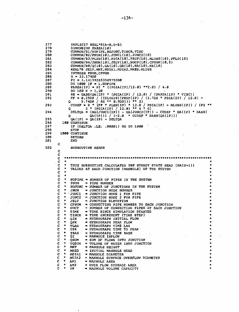
277 278 279 280 281 282 283 284 285 286 287 288 289 290 291 292
293
294
295 296 297 298 299 300 301
c 302
c c c c c c c c c c c c c c c c c c c c c c c c c c c c c c c c c c
-136-
IMPLICIT REAL*S(A-H,O-Z) DIMEllSION PAREA(l0) COMMON/Bl/NOPIPE,NOJUNC,TINCR,VISC COMMON/B2/PNUM(l0),JUNCl(l0),JUNC2(l0) COMMON/B3/PLEN(l0),PDIA(l0),PRUF(l0),MLOSS(l0),PFLO(l0) COMMON/B4/JNUM(l0),JELV(l0),NOCP(l0),CPNUM(l0,5) COMMON/BS/Q( 10) ,QA ( llil), QB ( 10), HA( 10). HB ( l 0) REAL*S JELV,MHT,MOIA1,MDI~2,MHED,MLOSS INTEGER PNUM,CPNUM G • 32.17400 PI• 3.14159265358979300 DO 1000 IP• l,NOPIPE PAREA(IP) •PI* {(POIA(IP)/12.0) **2.0) / 4,0 DO 100 N :::1 1,20 RB= DABS(QA(IP) * (PDIA(IP) / 12.0) / (PAREA(IP) * VISC)) FF• 0.2500 / ((DLOGlO((PRUF(IP) / (3.700 * PDIA(IP) / 12.0) +
Q . 5.7400 /RE •• 0,900))) ** 2) CCOEF • 8 *(FF* PLEN(IP) * 12.0 / PDIA(IP) + MLOSS(IP)) / (PI**
Q 2 * (PDIA(IP) / 12.0) •• 4 * G) DELTQA • (HA(JUNCl(IP)) - HA(JUNC2(IP)) - CCOEF * QA(IP) * DABS(
Q QA(IP))) / (-2.0 * CCOEF * DABS(QA(IP))) QA(IP) = QA(IP) - OELTQA
100 CONTINUE IF (DELTQA ,LE •• 00001) GO TO 1000 STOP
1000 CONTINUE RETURN ENO
SUBROUTINE HEADB
••••••••••••••••••••••••••••••••••••••••••••••••••••••••••••••••••••• * • * THIS SUBROUTINE CALCULATES THE STEADY STATE HEAD (HA(N+l)) * * VALUES AT EACH JutlCTION (MANHOLE) OF THE SYSTEM * • • • NOPIPE • PNUM • NOJUNC • JNUM * . JUNCl • JUNC2 • JELV • CPN!JM • NOCP • TIME • TINCR • QIN • QPK • TLAG • TPK • TBAS • QI • QSUM • TQSUM • MHT • MHEO • MDIAl • MDIA2 • A Ml • AM2 • VM
• NUMBER OF PIPES Itl THE SYSTEM = PIPE NUMBER a NUMBER OF 'JUtU:TIONS IN THE SYSTEM = JUNCTION NOOE NUMBER • JUNCTIOU NODE l FOR PIPE = JUNCTION NODE 2 FOR PIPE = JUNCTION ELEVATIO~ •. CONtlECTING PIPE NUMBER TO EACH JUNCTION
NUMBER OF CONNECTING PIPES AT EACH JUNCTION = TIME SINCE SIMULATION STARTED • TIME INCREIIENT (TIME STEP) • HYOROGRAPH INITIAL FLOW • HYOROGRAPH PEAK FLOW • HYOROGRAPH .TIME LAG • HYDROGRAPH TIME TO PEAK :::1 HYDROGRAPH TIME BASE • MANHOLE INFLOW = SUM OF FLOWS INTO JUNCTION ,. VOLUME OF WATER INTO .JUNCTION • MANHOLE HEIGHT • INITIAL MANHOLE HEAD • MANHOLE DIAMETER
MANHOLE SURFACE OVERFLOW DIAMETER • MANHOLE AREA • OVER FLOW STORAGE AREA = MAllHOLE VOLUME CAPACITY
• • • • • • • • • • * • • • • • • • • • • • • • • • • •
303 304 305 306 307 308 309 310 311 312 313 314 315 316 317 318 319 320 321 322 323 324 325 326
327 328
329 330 331 332 333 334 335 336 337 338 339 340 341 342 343 344 345 346 347 348 349 350 351 352 353 354
355
c c c c c c c c
c
• • • • • •
WHTl WHT WHT2 HA QA
-137-
• WATER HEIGHT AT JUNCTION FROM PREVIOUS TIME STEP = WATER HEIGHT ABOVE MANHOLE FROM PREVIOUS TIME STEP • WATER HEIGHT AT JUNCTION FOR PRESENT TIME STEP • JUNCTION HEAD FOR STEADY STATE FLOW CONDITIONS = STEADY STATE PIPE FLOW
• • • • • •
*********************************************************************
IMPLICIT REAL*B(A-H,0-Z) DIMEliSION QJ(5) COMMON/Bl/NOPIPE,NOJUNC,TINCR, VISC COMMON/82/PtlUM ( 10), JUNCl ( 10), JUUC2 ( 10) COMMON/B4/Jt1UM(l0),JELV(l0),NOCP(l0).CPNUM(l0,5) COMMON/BS/KEY( 10), MHT( 10), MDIAl (10), MDIA2 ( 10), MHED( 10) COMMON/B6/QI(l0),QIN(l0),QPK(l0),TLAG(l0),TPK(l0),TBAS(l0),TIME COMMON/B8/Q(l0),QA(l0),QB(lcr),HA(l0),HB(l0) REAL*8 JELV,MHT,MDIAl,MDIA2,MHEO,MLOSS INTEGER PNUM,CPNUM PI• 3.141592653589793D0 DO 150 IJ = l,NOJUNC IF (KEY(IJ) .EQ. 1) GC TO 140 NOCPS • NOCP(IJ) DO 30 N = l,NOCPS IF (JUNCl(CPNUM(IJ,N)) .EQ. IJ) GO TO 20 QJ(N) • QB(CPNUM(IJ,N)) GO TO 30
20 QJ(N) = 0.0 - QB(CPNUM(IJ,N)) 30 CONTINUE
IF (TIME IF (TIME IF (TIME OI(IJ) =
0 GO TO 60
.GT. TBAS(IJ)) GO TO 50
.GT. TPK(IJ)) GO TO 40
.LE. TLAG(IJ)) GO TO 50 QIN(IJ) + ((TIME-TINCR)/ (TPK(IJ) - TLAG(IJ))
TLAG(IJ)) * (OPK(IJ) - QUl(IJ))
40 QI(IJ) • QPK(IJ) + ((OIN(IJ) - QPK(IJ)) * ((TIME-TIHCR) - TPK(IJ)) 0 ./(TBAS(IJ) - TPK(IJ)))
GC TO 60 50 QI(IJ) = QIN(IJ) 60 QSUM • OI(IJ)
NOCPS = NOCP(IJ) DO 70 N • 1.tJOCPS
70 QSUM • QSUM + QJ(N) TQSUM = OSUM * TINCR AMl = PI • ((MDIAl(IJ) / 12.0) •• 2.0) / 4.0 VM =AM!* MHT(IJ) AM2 =PI• ((MDIA2(IJ)) •• 2.0) / 4.0 WHTl • HB(IJ) - JELV(IJ) IF (WHTl .GT. ~ll!T(IJ)) GO TO 90 TQSUM = TQSUM + WHTl * AMl IF (TQSUM .GT. VM) GO TO 100
80 WHT2 = TQSUM / AM! GO TO 120
90 WHT = WHTl - MHT(IJ) TQSUM =- TQSUM + MHT( IJ) * AMl + WHT * AM2 IF (TQSUM .LE. VM) GO TO 80
100 IIHT2 = MHT ( IJ) + ( TQSUM - VM) / AM2 120 HB(IJ) • WHT2 + JELV(IJ)
GO TO 150 140 Ql(IJ) = 0.0 150 CONTIUUE
RETURtl END
SUBROUTINE FLOWS
-138-
c c c c c c c c c c c c c c c c c c c c c c c c c c c c
~···································································· • * THIS SUBROUTINE CALCUIATES THE STEADY STATE FLOWRATE (QA(N+l)) * * IN EACH PIPE * • • • • • • • • • • • • • • • • • • • •
NOPIPE JUNCl JUNC2 HA QA PLEN PDIA PARE A PRUF MLOSS PFLO VISC G RE FF CCOEF OELTQA
• NUMBER OF PIPES IN THE SYSTEM = JUNCTION NODE l FOR PIPE = JUNCTION NODE .2 FOR PIPE • JUNCTION HEAD FOR STEADY STATE FLOl'I CONDTIONS • STEADY STATE PIPE FLOl'I • PIPE LENGTH • PIPE DIAMETER • PIPE AREA • PIPE ROUGHNESS (EPSILON) • SUM OF MINOR LOSSES = UIITIAL STEADY STATE PIPE FLOW • SYSTEM KINEMATIC VISCOSITY = ACCELERATION DUE TO GRAVITY • REYNOLDS NUMBER • DARCY FRICTION FACTOR (JAIN EQUATION) • HEAD LOSS COEFFICIENT = CHANGE IN STEADY STATE FLOWRATE
• • • • • • • • • • • • • • • • • • • •
*******************************************************W*************
356 IMPLICIT REAL*S(A-H,O-Z) 357 DIMENSION PAREA(95) 358 COMMON/Bl/NOPIPE,NOJUNC,TINCR,VISC 359 COMMON/B2/PNUM (HI), JUt,Cl (HI) ,JUNC2 (l0) 360 COMMON/B3/PLEN(l0), PDIA( l0), PRUF ( l0), MLOSS ( l0), PFLO( l0) 361 COMMON/B4/JNUM(l0),JELV(l0),NOCP(l0),CPNUM(l0,5) 362 COMMOtl/B8/Q( HI), QA( l0), QB ( Hl) ,HA( HI), HB ( l0) 363 REAL*B JELV,MHT,MOIA1,MDIA2,MHED,MLOSS 364 INTEGER PNUM,CPtiUM 365 G • 32.17400 366 PI= 3.14159265358979300 367 00 1000 IP• l,NOPIPE 368 PAREA(IP) •PI* ((PDIA(IP)/12.0) **2.0) / 4.0 369 RE= DABS(QB(IP) * (PDIA(IP) / 12.0) / (PAREA(IP) * VISC)) 370 FF= 0.2500 / ((DLOGl0((PRUF(IP) / (3.700 * PDIA(IP) / l2.0) +
Q 5.7400 /RE •• 0.900))) •• 2) . 371 CCOEF = 8 * (FF* PLEN(IP) * 12.0 / POIA(IP) + MLOSS(IP)) /(PI**
Q 2 * (POIA(IP) / 12.0) •• 4 * G) 372 OELTQB • TINCR * G *PI* (PDIA(IP) / 12.0) ** 2 * (HB(JUNCl(IP))
Q - HB(JUNC2(IP)) - CCOEF * QB(IP) * DABS(QB(IP))) / ( 4.0 Q * PLEN(IP))
373 QB(IP) • QB(IP) + DELTQB 374 1000 CONTINUE 375 RETURN 376 END
REFERENCES
1. American Society of Civil Engineers (ASCE) and Water Pollution Control Federation (WPCF), "Design and Construction of Sanitary Storm Sewers," ASCE Report No. 37, New York, 1969.
2. Bergeron, L., Water Hammer in Hydraulics and Wave Surges in Electricity, ASME, John Wiley and Sons, Inc., New York, 1961.
3. Bettes, R., Pitfield, R.A., .and Price, R.K., "A Surcharging Model for Storm Sewer Systems," Proceedings of The First International Conference on Urban Storm Drainage, Ed. by P.R. Helliwell, Wiley-Interscience, New York, 1978, PP• 306-316.
4. Brandstetter, A., "Assesment of Mathematical Models for Urban Storm and Combined Sewer Management," Environmental Technology Series, Muniipal Environmental Research Laboatory, US EPA, Aug. 1976.
5. Burke, C.B., and Gray, D.D., "A Comparative Application of Several Methods for the Design of Storm Sewer," Technical Report No. 118, Water Resources Research Center, Purdue University, West Lafayette, Indiana, Aug. 1979.
6. Chaudhry, M.H., Applied Hydraulic Tansients, Van Nostrand Reinhold Co., New York, 1979, pp. 44-73.
7. Chevereau, G., Holly, F.M., and Preismann, M.A., "Can Detailed Hydraulic Modeling be Worthwhile when Hydrologic Data is Incomplete?," Procceedigs of the First International Conference on Urban Storm Drainage, Ed. by P.R. Helliwell, WileyInterscience, New York, 1978, pp. 317-326.
8. Chow, v.T., and Yen B.C., "Urban Storm Runoff: Determination of Volumes and Flowrates," Environmental Protection Technology Series, Municipal Environmental Research Laboratory, US EPA, Cincinatti, Ohio, May 1978.
9. Cloyer, P.J., and Pethick, R.W., "Storm Drainage Design Methods: A Literature Review," Report No. INT 154, Hydraulics Research Station, Wallingford, England, March 1976.
10. Colebrook, C.F., "Turbulent Flow in Pipes with Particular Reference to the Transition Region Between the Smooth and Rough Pipe Laws," Journal of the Institute of Civil Engineers (London), Vol. 11, 1938-1939, PP• 133-156.
-139-
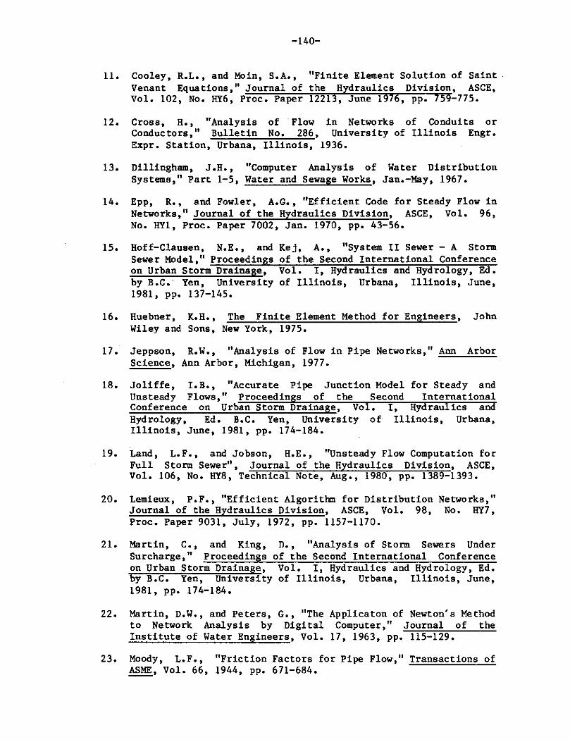
11.
12.
13.
-140-
Cooley, R.L., and Moin, S.A., Venant Equations," Journal of Vol. 102, No. HY6, Proc. Paper
"Finite Element Solution of Saint . the Hydraulics Division, ASCE, 12213, June 1976, PP• 759-775.
Cross, H., "Analysis of Flow in Networks of Conduits or Conductors," Bulletin No. 286, University of Illinois Engr • ..C....C--'---'----'---,-'----"'-'-'-Exp r. Station, Urbana, Illinois, 1936.
Dillingham, J.H., Systems," Part 1-5,
"Computer Analysis of Water and Sewage Works,
Water Distribution Jan.-May, 1967.
14. Epp, R., and Fowler, A.G., "Efficient Code for Steady Flow in Networks," Journal of the Hydraulics Division, ASCE, Vol. 96, No. HYl, Proc. Paper 7002, Jan. 1970, pp. 43-56.
15. Hoff-Clausen, N.E., and Kej, A., "System II Sewer - A Storm Sewer Model," _P_r_o_c_e_e_d_i_n~g~s_o_f_t_h_e_S_e_c_o_n_d_I=n_t_e_r_n_a_t_i_o_n_a_l_C=o_n_f_e_r_e=n_c_e on Urban Storm Drainage, Vol. I, Hydraulics and Hydrology, Ed. by B.c.· Yen, University of Illinois, Urbana, Illinois, June, 1981, PP• 137-145.
16. Huebner, K.H., The Finite Element Method for Engineers, John Wiley and Sons, New York, 1975.
17. Jeppson, R.W., "Analysis of Flow in Pipe Networks," Ann Arbor Science, Ann Arbor, Michigan, 1977.
18. Joliffe, I. B., "Accurate Pipe Junction Model for Steady and Unsteady Flows," Proceedings of the Second International Conference on Urban Storm Drainage, Vol. I, Hydraulics and Hydrology, Ed. B.C. Yen, University of Illinois, Urbana, Illinois, June, 1981, pp. 174-184.
19. Land, L.F., and Jobson, H.E., "Unsteady Flow Computation for Full Storm Sewer", Journal of the Hydraulics Division, ASCE, Vol. 106, No. HY8, Technical Note, Aug., 1980, pp. 1389-1393.
20.
21.
22.
Lemieux, P.F., "Efficient Algorithm for Distribution Journal of the Hydraulics Division, ASCE, Vol. 98, Proc. Paper 9031, July, 1972, pp. 1157-1170.
Networks," No. HY7,
Martin, C., and King, n., "Analysis of Storm Sewers Under Surcharge , " _P_r-=o_c_e-,e_d_i_n~g~s_o,,,f,.....,,t_h_e--::S,...e_c,,,o,...n_,d_I_n..,.t..,e_r_n_a_t_i_,o_n,,,a_l-,-_C..,.o_n_f_e_r_e,,,n_,c_e on Urban Storm Drainage, Vol. I, Hydraulics and Hydrology, Ed. by B.C. Yen, University of Illinois, Urbana, Illinois, June, 1981, pp. 174-184.
Martin, D.W., and Peters, G., "The to Network Analysis by Digital Institute of Water Engineers, Vol.
Applicaton of Newton's Method Computer," Journal of the
17, 1963, PP• 115-129.
23. Moody, L.F., "Friction Factors for Pipe Flow," Transactions of ~. Vol. 66, 1944, PP• 671-684.
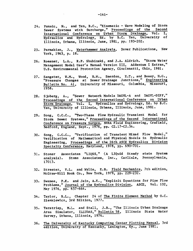
-141-
24. Pansie, N., and Yen, B.C., "Kinematic - Wave Modeling of Storm Sewer Systems with Surcharge," Proceedings of the Second International Conference on Urban Storm Drainage, Vol. I, Hydraulics and Hydrology, Ed. by B.C. Yen, University of Illinois, Urbana, Illinois, June, 1981, pp. 193-202.
25. Parmakian, J., Waterhammer Analysis, Dover Publications, New York, 1963, p. 18.
26. Roesner, L.A., R.P. Shubinski, and J.A. Aldrich. "Storm Water Management Model User's Manual Version III, Addentum I Extran, 11
U.S. Environmental Protection Agency, Cincinnatti, Ohio, 1981.
27. Sangster, W.M., Wood, H.W., Smerdon, E.T., and Bossy, H.G., "Pressure Changes at Sewer Drainage Junctions," Engineering Bulletin No. 41, University of Missouri, Columbia, Missouri, 1958.
28. Sjoberg, A., "Sewer Network Models DAGVL-A and DAGVL-DIFF," Proceedings of the. Second International Conference on Urban Storm Drainage, Vol. I, Hydraulics and Hydrology, Ed. by B.C. Yen, University of Illinois, Urbana, Illinois, June, 1981.
29. Song, c.c.c., "Two-Phase Flow Hydraulic Transient Model for Storm Sewer Systems," Proceedings of the Second International Conference on Pressure Surges, BHRA Fluid Engineering, Crafield, Bedford, England, Sept., 1976, pp. C2.17-C2.34.
30. Song, c.c.c., "Verification of Transient Mixed Flow Model," Verification of Mathematical and Physical Models in Hydraulic Engineering, Proceedings of the 26th ASCE Hydraulics Division Specialty Conference, Maryland, 1978, pp. 690-701.
31. Stoner Associates analysis). Stome 17013.
"LIQSS," Associates,
(A LIQuid Steady Inc., Carlisle,
state System Pennsylvania,
32. Streeter, V.L. and Wylie, E.B. Fluid Mechanics, 7th edition, McGraw-Hill Book Co., New York, 1979, pp. 229-232.
33. Swamee, P.K. and Jain, A.K., "Explicit Equations for Problems," Journal of the Hydraulics Division, ASCE, May 1976, pp. 657-664.
Pipe Flow Vol. 102,
34. Taylor, R.L., Chapter 24 of The Finite Element Method by O.C.
35.
Zienkiewicz, 3rd Edition, 1977.
Terstriep, M.L. and Stall, J.B., "The Area Simulator, ILLUDAS," Bulletin 58, Survey, Urbana, Illinois, 1974.
Illinois Urban Drainage Illinois State Water
36. The University of Kentucky Computing Center Plotting Manual, 3rd edition, University of Kentucky, Lexington, Ky., June 1981.
-142-
37. Tholin, A.L. and Keifer, C.J., "The Hydrology of Urban Runoff," Transactions, ASCE, Vol. 125. 1960, pp. 1308-1379.
38. Thorley, A.R.D., Twyman, J.W.R. Introduction to Pressure Surge, Dept. The City University, London, England,
and Enever, of Mechanical April 1975.
K.J., An Engineering,
39. Toyokuni, E., "Stormwater Runoff with Surcharge in Matsuyama City", Proceedings of the Second International Conference on Urban Storm Drainage, Vol. I, Hydraulics and Hydrology, Ed. by B.C. Yen, University of Illinois, Urbana, Illinois, June 1981, PP• 203-212.
40.
41.
Wallker, Hammer," p. 764.
M.L., Jr., et al, "Viscious Dispersion in Water Transactions, ASME, Journal of Basic Engineering, 1960,
Watkins, L.H., "A Guide for Engineers to the Design Sewer Systems," Road Research Technical Paper No. 55, Science and Industry Research, Great Britain, 1963.
of Storm Dept. of
42. Wood, D.J., Dorsch, R.G. and Lightner, C., "Wave-Plan Analysis of Unsteady Flow in Closed Conduits," Journal of the Hydraulics Division, ASCE, Vol. 92, No. HY2, Proc. Paper 4716, March 1966, PP• 83-110.
43. Wood, D.J., "An Explicit Friction Factor Relationship," Civil Engineering, ASCE, Vol. 36, No. 12, Dec. 1966, pp. 60-61.
44. Wood, D.J. and Charles, C .o.A., "Hydraulic Network Analysis Using Linear Theory," Journal of the Hydraulics Division, ASCE, Vol. 98, No. HY7, Proc. Paper 9031, July 1972, pp. 1157-1170.
45. Wood, D.J., "The Analysis of Flow in Surcharged Storm Sewer Systems," Proceedings, International Symposium on Urban Storm Runoff, Lexington, Kentucky, July 1980, pp. 29-35.
46. Wood, D.J., ''Users Manual - Computer Analysis of Flow in Pipe Networks Including Extended Period Simulations,". Office of Continuing Education, University of Kentucky, Lexington, Kentucky, Sept. 1980.
47. Wood, D.J., "Water Hammer Analysis in Pipe Systems Method, A Computer Program for Transient Pipe Flow Dept. of Civil Engr., University of Kentucky, Kentucky, May 1981.
- Wave Plan Analysis," Lexington,
48. Wylie, E.B., and Streeter, v.L., Fluid Transients, McGraw-Hill Inc., New York, 1978.
49. Yen, B.C., Wenzel,H.G., Mays, L.W., and Wilson, H.T., Methodologies for Design of Storm Sewer Systems," Report No. 112, Water Resources Center, Un\versity of Urbana, Illinois, August 1976.
"Advanced Research
Illinois,

-143-
50. Yen, B.C., "Hydraulic Instabilities of Storm Sewer Flows," Proceedings of the First International Conference on Urban Storm Drainage, Ed. by P.R. Helliwell, Wiley-Interscience, New York, 1978, PP• 282-293.
51. Yen, B.C., (ed.), Storm Sewer System Design, Dept. of Civil Engr., University of Illinois, Urbana, Illinois, 1978.
52. Yen, B.C. and Pansie, N., "Surcharge of Sewer Systems," Research Report No. 149, Water Resources Center, University of Illinois, Urbana, Illinois, March 1980.
53. Yev jevich, V. and Barnes, A.H., "Flood Routing Through Flood Drains," Parts I-IV, Hydrology Papers, Colorado State University, Fort Collins, Colorado, Nov. 1970.
54. Zienkiewicz, o.c., The Finite Element Method in Engineering Science, McGraw-Hill Inc., London, England, 1977.