hydrogen production and delivery infrastructure as …
TRANSCRIPT

HYDROGEN PRODUCTION AND
DELIVERY INFRASTRUCTURE
AS A COMPLEX ADAPTIVE SYSTEM
RCF Economic and Financial Consulting, Inc.
Argonne National Laboratory
Final Report
Award Number DE-FG36-05GO15034
June 2010
TABLE OF CONTENTS
PREFACE ........................................................................................................................................ i ACKNOWLEDGEMENTS ........................................................................................................... iii ABSTRACT ................................................................................................................................... iv
EXECUTIVE SUMMARY ............................................................................................................ 1
PART ONE: INTRODUCTION
1.1 Purpose of the Present Project .......................................................................................... 10
1.2 Approach of this Project ................................................................................................... 10
1.3 Relation of this Project to Other Applied Agent-based Modeling Work .......................... 11
1.3.1 Range of Applications................................................................................................ 11
1.3.2 Institutes Devoted to Agent-based Modeling Applications ....................................... 11
1.3.3 Industry Applications ................................................................................................. 12
1.4 Outline of Report .............................................................................................................. 13
PART TWO: THE MODEL
2.1 Overview of Model ........................................................................................................... 15
2.1.1 Introduction of Players ............................................................................................... 15
2.1.2 Description of Model Area ........................................................................................ 16
2.1.3 Model Simulation Steps ............................................................................................. 17
2.2 Driver Agents .................................................................................................................... 18
2.2.1 Driver Population ....................................................................................................... 18
2.2.2 Vehicle Purchasing and the Driver Utility Function .................................................. 19
2.2.3 Vehicle Refueling ...................................................................................................... 21
2.3 Investor Agents ................................................................................................................. 22
2.3.1 Hydrogen Fuel Production Technologies .................................................................. 23
2.3.2 Price Charged for Hydrogen Fuel .............................................................................. 27
2.3.3 Station Siting .............................................................................................................. 27
2.3.4 Financial Evaluation of the Investment Plan ............................................................. 30
2.3.5 Number of Investors .................................................................................................. 34
PART THREE: SENSITIVITY TO MODEL PARAMETERS
3.1 Benchmark Case ............................................................................................................... 35
3.1.1 Parameter Values for the Benchmark Case ............................................................... 36
3.1.2 Hydrogen Vehicle Sales Penetration ......................................................................... 38
3.1.3 Hydrogen Vehicle Stock Penetration ......................................................................... 39
3.1.4 Hydrogen Fuel Station Penetration ............................................................................ 40
3.1.5 Location of Fuel Stations ........................................................................................... 41

3.1.6 Investor Agent Cumulative Cash Flows .................................................................... 41
3.2 Driver Sensitivity Scenarios ............................................................................................. 42
3.2.1 Driver Familiarity ...................................................................................................... 42
3.2.2 Bandwagon Effect ...................................................................................................... 44
3.2.3 Greenness ................................................................................................................... 45
3.2.4 Conclusions on Model Sensitivity to Driver Behavior .............................................. 48
3.3 Investor Sensitivity Scenarios ........................................................................................... 49
3.3.1 Investor Discount Rate - Staff.................................................................................... 49
3.3.2 Investor Discount Rate - Upper Management ........................................................... 50
3.3.3 Rapidity of Learning .................................................................................................. 51
3.3.4 First Year Demand Estimation at Potential Station Locations .................................. 52
3.3.5 Expectation of Growth ............................................................................................... 54
3.3.6 Number of Investors .................................................................................................. 55
3.3.7 Conclusions on Model Sensitivity to Investor Behavior ........................................... 56
3.4 Use of Realistic Approximative Decisions ....................................................................... 57
PART FOUR: SENSITIVITY TO MARKET AND POLICY INFLUENCES
4.1 Market Developments: Sticker Price Difference ............................................................. 59
4.1.1 Constant Sticker Price Difference .............................................................................. 59
4.1.2 Declining Sticker Price Difference ............................................................................ 60
4.2 Market Developments: Fuel Prices .................................................................................. 62
4.3 Policies: Tax Credits for Hydrogen Vehicle Purchase .................................................... 64
4.3.1 Permanent Tax Credit ................................................................................................ 65
4.3.2 Temporary Tax Credit ................................................................................................ 65
4.4 Policies: Carbon Taxes .................................................................................................... 67
4.5 Policies: Seed Stations ..................................................................................................... 68
4.6 Conclusions ....................................................................................................................... 71
PART FIVE: VALIDATION
5.1 Relation of Adoption Paths of this Study to Previously Estimated Adoption Paths ........ 72
5.1.1 The Logistic Function and the Comparison of Adoption Paths ................................. 73
5.1.2 Comparison of Hydrogen Vehicles with Consumer Durables as a Whole ................ 74
5.2 Adoption Experience under Other Vehicle Information ................................................... 76
5.2.1 Compressed Natural Gas Vehicles............................................................................. 76
5.2.2 The Market Penetration of Japanese Vehicles in the United States ........................... 79
5.2.3 Hybrid Vehicles ......................................................................................................... 82
5.3 Conclusions on Validation ................................................................................................ 87

PART SIX: SUMMARY AND CONCLUSIONS
6.1 The Agent-Based Model ................................................................................................... 88
6.2 Benchmark Case ............................................................................................................... 88
6.3 Sensitivity to Driver Behavior .......................................................................................... 89
6.4 Sensitivity to Investor Behavior ....................................................................................... 90
6.5 Effect of Realistic Approximative Decisions in the Agent-based Model ......................... 90
6.6 Use of the Model to Examine Market Developments ....................................................... 91
6.7 Policies .............................................................................................................................. 92
6.8 Model Validation .............................................................................................................. 93
6.9 Bottom Line Issue of this Study: Adequacy of Private Sector Infrastructure Supply ..... 93
6.10 Future Work ..................................................................................................................... 94
APPENDIX A: DRIVER MODULE ........................................................................................... 96 APPENDIX B: INVESTOR MODULE .................................................................................... 108 APPENDIX C: FACTORS AFFECTING FUTURE COSTS OF PRODUCING HYDROGEN
VEHICLES ...................................................................................................... 121
i
PREFACE
In 2005, the Hydrogen, Fuel Cells and Infrastructure Technologies Program of the Office
of Energy Efficiency and Renewable Energy of the U.S. Department of Energy contracted with
RCF Economic and Financial Consulting, Inc. to develop an Agent-based Model (ABM), in
cooperation with Argonne National Laboratory, on the construction of hydrogen infrastructure as
hydrogen vehicles penetrate the U.S. light-duty vehicle market. Industry cooperators were Ford
Motor Company, BP, Protium Energy Technologies, and John E. Johnston (formerly Planning
Executive for ExxonMobil's Corporate Strategic Research Laboratories).
A principal product of this project is the agent-based model ―Hydrogen Infrastructure
Complex Adaptive Systems‖ (H2CAS). The model benefitted from earlier work on other topics
using agent-based modeling at the Center for Energy, Environmental, and Economic Systems
Analysis (CEEESA) at Argonne National Laboratory, and from a similar model previously
developed at Ford Motor Company. Conventional methods to address technology introduction
rely on traditional optimization procedures such as simple cost minimization assuming perfect
knowledge. There are too many interactions among the participating entities in the hydrogen
transition to be captured with these techniques. The agent-based model simulates the behavior
and interactions of a large number of individuals (agents) and studies the macro-scale
consequences of these interactions. The agents represent a diverse group of actors with different
tastes, resources, strategies, and risk preferences. Agents use rules of thumb and other realistic
informal estimation techniques. They may be biased. Corrective actions occur as agents learn
from their experience. They adapt over time.
The study team was charged with answering the questions, ―Will the private sector be
likely to undertake this infrastructure investment on its own, and with sufficient promptness to
satisfy national energy and foreign policy goals?‖ and ―If not, what policy actions would be
effective?‖
To answer these questions, projections are given of how hydrogen infrastructure will
grow and how hydrogen vehicles will penetrate the market under alternative conditions.
Sensitivity scenarios are presented pertaining to such influences as the cost of hydrogen vehicles
relative to non-hydrogen vehicles, the price of gasoline, risk attitudes of senior managers at
companies involved in hydrogen supply technologies, and behavior of consumers. The
effectiveness of policies that would affect adoption is estimated.
Part One introduces the report and discusses other applications of agent-based modeling.
Part Two gives an overview of the model. The model offers the ability to introduce a
variety of characteristics of people who might purchase hydrogen vehicles (driver agents). On
the infrastructure side of the problem, the agent-based approach allows the firms that provide
hydrogen for vehicles (investor agents) to make investment decisions that are not strictly
maximizing. Instead they use satisficing rules of thumb and other approximations, making
decisions that are ―good enough‖ if not perfect. This allows investor agents to behave more like
real business people, who face circumstances that are too complicated to allow perfect maximize.

ii
Part Three reports simulation results of the model with, first, a benchmark set of
parameters and then with variations allowing study of sensitivity to numerical values of model
parameters.
Part Four reports results of simulations examining a number of market and policy
parameters, including the sticker price of the hydrogen vehicle, vehicle fuel prices, tax credits,
carbon taxes, and seed stations at the beginning of the simulation provided with policy help.
Part Five is concerned with validation. The simulations of the present study are compared
to experiences with a number of other innovations, many of which have encountered chicken-or-
egg effects that characterize the introduction of hydrogen. The investigation includes a variety
of consumer durables plus experiences with compressed natural gas vehicles, Japanese imports,
and hybrid vehicles.
Part Six summarizes the results of the study and draws conclusions regarding ability to
supply infrastructure that will permit market penetration of hydrogen vehicles..
Technical appendices report the mathematical structure of the driver module (Appendix
A) and investor module (Appendix B) and summarize major influences on the future price of
hydrogen vehicles (Appendix C).

iii
ACKNOWLEDGEMENTS
The team at RCF was led by George Tolley and included Donald Jones, Naveen Singhal,
Mihai Sturdza, Catherine Mertes, Mark Grenchik, David Jarvis, and several other RCF staff
members. The team at Argonne National Laboratory was led by Guenter Conzelmann, and
included Marianne Mintz, Craig Stephan (formerly of Ford), Matthew Mahalik, Thomas
Veselka, and Audun Botterud. The hydrogen model made use of the Argonne team’s experience
with agent-based modeling and an earlier model of hydrogen vehicle adoption developed at Ford
Motor Company by Craig Stephan and John Sullivan.
Generous and valuable contributions were made by the industry cooperators, who
included Dean Fry of BP; Craig Stephan and John Sullivan of Ford Motor Company; John
Johnston formerly of ExxonMobil; and Venki Raman of Protium Energy Technologies.
Very helpful comments on the draft report were provided by the peer reviewers, who
were Shannon Baxter-Clemmons of the South Carolina Hydrogen and Fuel Cell Alliance, Maria
Curry-Nkansah of the Imago Energy Consultancy Group, and George Parks of FuelScience LLC.
Fred Joseck of DOE was a constant source of valuable feedback and help. Midterm
decisions benefitted greatly from comments in semi-annual Fuel Pathways Integration Technical
Team (FPITT) meetings in Washington, D.C., Golden, CO, and Naperville, IL over the course of
the project.

iv
ABSTRACT
An agent-based model of the transition to a hydrogen transportation economy explores
influences on adoption of hydrogen vehicles and fueling infrastructure. Attention is given to
whether significant penetration occurs and, if so, to the length of time required for it to occur.
Estimates are provided of sensitivity to numerical values of model parameters and to effects of
alternative market and policy scenarios. The model is applied to the Los Angeles metropolitan
area
In the benchmark simulation, the prices of hydrogen and non-hydrogen vehicles are
comparable. Due to fuel efficiency, hydrogen vehicles have a fuel savings advantage of 9.8
cents per mile over non-hydrogen vehicles. Hydrogen vehicles account for 60% of new vehicle
sales in 20 years from the initial entry of hydrogen vehicles into show rooms, going on to 86% in
40 years and reaching still higher values after that. If the fuel savings is 20.7 cents per mile for a
hydrogen vehicle, penetration reaches 86% of new car sales by the 20th
year. If the fuel savings
is 0.5 cents per mile, market penetration reaches only 10% by the 20th
year. To turn to vehicle
price difference, if a hydrogen vehicle costs $2,000 less than a non-hydrogen vehicle, new car
sales penetration reaches 92% by the 20th
year. If a hydrogen vehicle costs $6,500 more than a
non-hydrogen vehicle, market penetration is only 6% by the 20th
year. Results from other
sensitivity runs are presented.
Policies that could affect hydrogen vehicle adoption are investigated. A tax credit for the
purchase of a hydrogen vehicle of $2,500 tax credit results in 88% penetration by the 20th
year,
as compared with 60% in the benchmark case. If the tax credit is $6,000, penetration is 99% by
the 20th
year. Under a more modest approach, the tax credit would be available only for the first
10 years. Hydrogen sales penetration then reach 69% of sales by the 20th year with the $2,500
credit and 79% with the $6,000 credit.
A carbon tax of $38 per metric ton is not large enough to noticeably affect sales
penetration. A tax of $116 per metric ton makes centrally produced hydrogen profitable in the
very first year but results in only 64% penetration by year 20 as opposed to the 60% penetration
in the benchmark case. Provision of 15 seed stations publicly provided at the beginning of the
simulation, in addition to the 15 existing stations in the benchmark case, gives sales penetration
rates very close to the benchmark after 20 years, namely, 63% and 59% depending on where they
are placed.

1
EXECUTIVE SUMMARY
INTRODUCTION
This final report presents results of the Analysis of the Hydrogen Production and
Delivery Infrastructure as a Complex Adaptive System (Award Number E-FC36-05GO15034),
conducted for the Fuel Cell Technologies Program of the Office of Energy Efficiency and
Renewable Energy of the U.S. Department of Energy.
The project is concerned with the ability to provide infrastructure necessary to support a
hydrogen transportation system. The start-up of a hydrogen transportation system encounters a
chicken-or-egg problem of what comes first, drivers of hydrogen cars or investors in hydrogen
fueling infrastructure. The central purpose is to answer:
Whether the private sector will supply the infrastructure to permit
a transition to hydrogen consistent with national goals and, if not,
what policy actions would be effective.
APPROACH
The methodology used is Agent-based Modeling (ABM). ABM actors use realistic
approximations in making decisions, rather than using perfect optimization that assumes
impossible requirements of complete knowledge. ABM permits the introduction of great variety
in the analysis of interactions among the many different actors in an economic system. The
model in this study was developed jointly between RCF Economic and Financial Consulting,
Inc. and Argonne National Laboratory.
The model simulates the interactions of drivers of hydrogen vehicles and investors
providing hydrogen fueling infrastructure, during years when adoption of hydrogen vehicles is
occurring. It provides a tool for estimating how different circumstances will affect the growth of
the hydrogen economy.
OUTLINE OF REPORT
Part One of the report provides an introduction. Part Two provides an overview of the
model including a description of the geographic area, driver agent and investor agent behavior,
the model simulation process, hydrogen production technology, and the hydrogen fuel station
siting process. Part Three describes the study’s benchmark adoption scenario and reports on
sensitivity to numerical estimates of driver and investor behavioral parameters. Part Four reports
on the sensitivity to market influences and policies. Part Five is concerned with validation of the
model through comparison of its prediction of hydrogen vehicle adoption with observed adoption
of previous innovations for durable goods. Part Six summarizes the major empirical findings of
the study, presents conclusions on the central question of prospects for adequate provision of
hydrogen infrastructures, and discusses the usefulness of the study in the future. Appendix A
contains further details regarding driver agents. Appendix B contains further on investor agents.
2
Appendix C presents an analysis of the sources of declines in cost of producing hydrogen
vehicles that would allow them to enter the mass market.
OVERVIEW OF THE MODEL
As discussed in Section 2.1, the Agent-based Model (ABM) developed for the study
contains 130 parameters which consist of 92 cost parameters from DOE’s H2A model, 17 driver
behavior parameters, 10 investor behavior parameters, and 11 price and policy variables.
The model area is a 100-by-50-mile rectangular area centered on the Los Angeles,
California, metropolitan area. Within the model area, there are two types of agents: potential
buyers of hydrogen vehicles (driver agents) and potential investors in hydrogen fuel
infrastructure (investor agents).
Driver agents make decisions regarding whether or not to purchase hydrogen vehicles
each quarter within each simulation year. At the beginning of a simulation, driver agents own
only non-hydrogen vehicles. Driver agents observe the few hydrogen fueling stations which are
sited as seed stations as part of the model. Driver agents then decide whether to replace their
non-hydrogen vehicles with hydrogen-powered vehicles depending on their individual
differences and on the location of stations where they can buy hydrogen fuel. Those hydrogen
vehicles are then fueled throughout the simulation year. Investor agents observe the fueling
behavior of driver agents, revise their expectations regarding the strength of demand based on
the sales they observe, and then decide where and how many new fuel stations to build in the
next simulation year. Driver agents then view the stations that have been added and once again
make decisions about purchasing hydrogen vehicles. The process repeats for each year of the
simulation.
DRIVER AGENTS
As discussed in Section 2.2, driver agents represent vehicle drivers living and working in
the model area. The driver agents live and work in different locations, have different incomes,
varying knowledge about hydrogen vehicles, varying attitudes toward the environment, and other
characteristics. Drivers differ in their proclivities to buy hydrogen vehicles and in their
proximity to hydrogen stations. The adoption path of hydrogen vehicles will depend on how
driver agents react to hydrogen fuel stations supplied by investor agents.
The model contains approximately 7 thousand drivers, each representing 1,000 vehicles in
order to approximate 7 million vehicles in the model area. At the beginning of the simulation,
nearly all driver agents own only conventional vehicles. In each simulation, drivers make trips,
refueling as needed. Drivers replace some part of the vehicle fleet each period during a
simulation, using the driver utility function to determine whether they would consider
themselves better off with a new hydrogen vehicle or another non-hydrogen vehicle.
The driver agent utility function has seven terms:
1. Sticker price difference

3
2. Fuel cost advantage
3. Disadvantage due to limited familiarity
4. Bandwagon effect
5. Greenness
6. Inconvenience
7. Worry
The sticker price difference is the price of a hydrogen vehicle minus the price of a
comparable non-hydrogen vehicle. The fuel cost advantage is the present value of any fuel cost
savings resulting from driving a hydrogen vehicle. The disadvantage due to limited familiarity
results from a driver agent’s hesitation to purchase a hydrogen vehicle due to a lack of
knowledge about it. The bandwagon effect occurs when a potential buyer’s beliefs about the
performance of a new product are influenced by those who have already purchased the product.
Greenness represents driver agent preferences, if any, toward hydrogen vehicles due to
environmental considerations. Inconvenience may result from a limited availability of hydrogen
refueling options. Worry may result from concern for running out of fuel because of limited
availability of hydrogen refueling options.
When few hydrogen stations are available in early periods, inconvenience and worry figure
noticeably in utility calculations. As a simulation proceeds, more fueling stations are sited and
these concerns lessen. As drivers buy hydrogen vehicles, other drivers who are able to observe
their performance become more comfortable with them in subsequent periods as the
disadvantage due to unfamiliarity is reduced.
INVESTOR AGENTS
As discussed in Section 2.3, investor agents supply the hydrogen infrastructure necessary
for refueling hydrogen vehicles purchased by the driver agents. Investor agents cannot foresee
hydrogen fuel sales with certainty. Realistically investors must resort to simplifications and
approximations. These are a central feature of the model in the present study, providing a
contrast to many traditional economic theories that assume perfect foresight or depart from
reality in modeling behavior toward the future in other ways. The simplifications and
approximations take a variety of forms. They include back-of-the-envelope calculations and
rules of thumb. An investor agent is subject to over- or under-optimistic biases. An investor
learns from experience and may change in degree of optimism or pessimism from one period to
the next. Decisions are influenced by broader corporate goals of upper management, such as
near-term earnings performance that affects share values of the company regardless of the long-
term promise of an investment. The terms satisficing and bounded rationality are sometimes
used to describe these types of influences on decisions departing from the assumption of perfect
maximization.
HYDROGEN PRODUCTION TECHNOLOGIES
Also discussed in Section 2.3, several potential hydrogen production technologies were
evaluated during this study. The major technologies included in the model are distributed stream
methane reforming and centralized stream methane reforming. Alternative technologies include

4
electrolysis, coal gasification and biomass gasification. Steam methane reforming (SMR)
consists of heating methane to 700o - 1,100
o C which separates it into carbon monoxide and
hydrogen.
Steam methane reforming is used in the model because our evaluation shows that it is the
most likely hydrogen production technology for the model area centered on the Los Angeles
metropolitan area. H2A models indicate that SMR is less expensive than either electrolysis or
coal gasification. It is unlikely that sufficient volumes of biomass would be available to produce
all the hydrogen needed in the latter years of the simulation via biomass gasification. Analysis in
this study indicates that switching technologies midway through the simulation period, from
biomass to SMR, would entail a higher cost than starting with SMR. Modeling the use of both
biomass gasification and SMR is possible but is beyond the scope of the present study.
With distributed SMR production, small reforming units are located at each refueling site.
With centralized SMR production, a large reformer serves many refueling sites by pipeline or
truck delivery.
The investor faces a choice between building distributed SMR stations, and building
centralized plants along with a pipeline infrastructure for delivery of fuel. To make the choice
between the two technologies, the investor compares the levelized cost of producing hydrogen
using the centralized technology with the levelized cost using distributed stations. Investor
agents choose the method of production based on projected sales volume and the lowest-cost
method for that volume. The investor charges a price for fuel that is equal to the average cost of
producing hydrogen.
STATION SITING
As further discussed in Section 2.3, the model area is divided into 5,000 1x1-mile cells.
The investor agent is restricted to siting stations in 156 cells located at major highway
intersections and at the midpoints of highway segments. Each cell may have as many stations as
the investor chooses to site there.
In the first year of the simulation, it is assumed there are only seed stations. Investor
agents consider siting stations annually from the second year onward. The procedure used to
make decisions regarding how many stations to site and at which locations uses a process to
forecast the expected hydrogen fuel sales and profitability of all possible new station locations,
ranks locations, and calculates the effect of siting a station. The procedure is repeated each year
of the simulation for all possible new station locations.
THE BENCHMARK SCENARIO
As discussed in Section 3.1, the benchmark case represents a 40 year scenario where
hydrogen vehicles and fuel become competitive with traditional vehicles. The benchmark case
provides an example of a set of prices of vehicles and fuels for hydrogen and non-hydrogen
vehicles that would result in cost competitiveness and allow the beginning of a take-off. It is to
be emphasized that the model does not attempt to predict the exact year when the required

5
competitiveness will be achieved. The benchmark scenario is presented as a baseline estimate
using the parameters in the following table:
Main Parameters Used in Benchmark Scenario
Parameter Value
Driver Agent Parameters
Disadvantage Due to Limited Familiaritya,f
$12,000
Bandwagon Effect Coefficient a 0.1
Bandwagon Effect Dispersion a 2.2
Greenness Central Tendencyb,f
$250
Greenness Dispersionb 10
Investor Agent Parameters
Fueling Station Capital Costc,f
$4,806,357
Fueling Station Fixed O&M Costsc,f
$236,598
Fueling Station Salvage Valuec 0
Investor Discount Rated 10%
Hydrogen Selling Pricee,f
$3.63/kg
Fueling Station Operating Capacityc 1,278 kg/day
a
For additional discussion see Section A.2.3 in Appendix A, ―Disadvantage Due to Limited
Familiarity and Bandwagon Coefficient, F
jtP and qj.‖
b For additional discussion see Section A.2.4 in Appendix A, ―Greenness, Tj.‖
c Station nameplate capacity of 1,500 kg/day from DOE H2A model.
d DOE H2A model.
e For additional discussion see Section B.1 in Appendix B, ―Price Charged for Hydrogen Fuel.‖
f In 2009 dollars.
Using these baseline estimates, the figure below shows annual hydrogen vehicle sales as
a percent of all light-duty vehicle sales over a forty year simulation period. Hydrogen vehicle
sales under the benchmark scenario reach a market penetration of 86% after 40 years.

6
Benchmark Hydrogen Vehicle Sales Penetration over 40 Years
0%
20%
40%
60%
80%
100%
0 5 10 15 20 25 30 35 40
Year
Per
cen
tag
e o
f L
igh
t-D
uty
Veh
icle
Sa
les
SENSITIVITY TESTING FOR DRIVER BEHAVIOR PARAMETERS
As discussed in Section 3.2, results of sensitivity analyses for the driver agents show that
driver agent behavior can have a significant effect on the rate at which hydrogen vehicles are
adopted. The strength of the disadvantage due to limited familiarity has a large initial influence
acting to slow sales growth, which is overcome over time due importantly to the bandwagon
effect or the impact of drivers who have already bought a hydrogen vehicle on drivers who have
not bought one yet. The influence of greenness or driver willingness to pay a premium for an
environmentally friendly vehicle is somewhat smaller but still significant.
SENSITIVITY TESTING FOR INVESTOR BEHAVIOR PARAMETERS
As discussed in Section 3.3, results of the sensitivity analyses for investor agents show
that the upper management discount rate can have a large influence on the number of fuel
stations built and consequently on hydrogen vehicle sales. The upper management discount rate
reflects the attitudes of investors including degree of risk aversion, and the degree of optimism or
pessimism about the viability of hydrogen vehicle expansion. In contrast, sensitivity of the
model to the staff discount rate used in preparing investment evaluations submitted for
consideration by upper management appears to be relatively small, because the staff uses a
narrower range of textbook discount rates. Relatively limited effects are also found for
sensitivity to the investor’s rapidity of learning, method of predicting first year sales at new
stations, and method of forming growth expectations. All the latter may have large effects for

7
one year, particularly early in the simulation when investor experience is limited, but the
unfolding of actual events corrects investor mistakes relatively rapidly. The number of investors
has a limited effect because a single investor is already acting much like a pure competitor in
view of the threat of entry of other investors and of regulation if monopolistic practices are
observed.
EFFECTS OF REALISTIC APPROXIMATIVE DECISIONS
Section 3.4 asked: What is the effect of realistic, approximative decision making,
sometimes called satisficing, in place of traditional, full optimization on the results? Obtaining a
strict answer is not feasible because calculating the fully optimized path would be impossibly
complicated. However, having perfect information about the growth rate of demand for
hydrogen, and about fueling locations with the greatest potential for spurring hydrogen vehicle
adoption, would eliminate important complications. An upper bound on these effects can be
obtained by re-running the simulation assuming that hydrogen stations are found at every
location. The lack of availability of hydrogen would then not be a hindrance to adoption.
The effect of the investor’s lack of perfect knowledge about demand in delaying the
provision of infrastructure would no longer be operative. Adoption of hydrogen vehicles would
still not be instantaneous because drivers would still have to learn about the performance of
hydrogen vehicles, which is the driver’s contribution to delay in adoption, not the investor’s. If
we compare the hydrogen vehicle saturation level at a given year, say the 20th
, in the re-run
simulation with that in the original simulation, we obtain an estimate of the maximum possible
delay that the investor’s satisficing behavior has caused. The results of the comparison reveal
that the maximum possible effect is a relatively modest 2-year delay by the 20th
year.
SENSITIVITY TESTING FOR POLICY AND MARKET INFLUENCES
Part Four reports on sensitivity scenarios for policy and market influences. The market
influences studied include changes to the sticker price of hydrogen vehicles, and changes to the
price of gasoline. Additional market changes not foreseen at the present time will inevitably
occur in the future. The model of this study can be useful beyond providing a prediction of
future conditions as seen at the present time. Sensitivity of model results to differences in
market conditions indicates how model results will be affected by different market conditions as
they emerge in the future, increasing the value of the study as a tool for use beyond the year of
the present study. The policy scenarios studied include tax credits for hydrogen vehicle
purchase, loan assistance to investors, the effect of possible carbon taxes, and additional seed
stations.
Market Developments: Sticker price differences (Section 4.1) have important effects on
the adoption of hydrogen vehicles. A decline sticker price disadvantage beginning with a
$14,000 hydrogen vehicle price disadvantage that declines to $0 by year 5 or 10 still allows sales
penetrations over 50% by the 20th
year. A non-declining price disadvantage of $6,500 precludes
a hydrogen take-off.
8
Market Developments: Fuel cost savings (Section 4.2) play an important role in the
adoption of hydrogen vehicles. Sufficiently low savings will prevent take-off, while very high
savings will hasten a take-off. The results are driven by the price of gasoline and suggest that
future gasoline prices could be a crucial market consideration determining hydrogen vehicle
penetration.
Policies: Permanent tax credits (Section 4.3.1) dramatically hasten sales penetration.
Temporary tax credits (Section 4.3.2) that end after 10 years still result in higher sales than in the
benchmark case with no tax credits, because so many more hydrogen vehicles are purchased
earlier and, operating through the bandwagon and familiarity effects, continue to affect vehicle
choice after the expiration of the tax credits.
Policies: Carbon taxes (Section 4.4) have limited effects. An additional 15 stations
available at the beginning of the simulation has a perceptible, though not major, but alternative
locations of the seed stations have little impact on sales penetration.
MODEL VALIDATION
As discussed in Part Five, research was conducted on adoption of other durable goods
innovations to see if the adoption path predicted for hydrogen vehicles in this study is similar to
those for other innovations. A comparative study was conducted on the adoption paths of
consumer durables products as a whole. Adoption experiences and lessons learned were
gathered for specific vehicle innovations including CNG vehicles, penetration of Japanese
vehicles in the U.S. market, and hybrid vehicles.
Overall, we judge the validation tests to be favorable to the Agent-based model of this
study. The adoption paths for hydrogen vehicles in the simulations of this study have been found
to have a typical S-shaped adoption curve similar to the empirical adoption paths calculated for
other consumer durables. The S-curve for hydrogen vehicles exhibits a slower rate of adoption
than for the average of all consumer durables. This is to be expected because automobiles
including hydrogen vehicles have a much longer life and are thus subject to slower turnover than
other durable goods. A lesson from the three vehicle case studies (CNG vehicles, Japanese
vehicles, and hybrids) is that gain to the consumer from an innovation and, in the case of
Japanese imports, government policy can have a powerful influence on the rate of adoption.
BOTTOM LINE ISSUE OF THIS STUDY: ADEQUACY OF PRIVATE SECTOR
INFRASTRUCTURE SUPPLY
In addition to summarizing the study, Part Six takes stock of the implications of the study
for the key question (Section 6.9): Will the private sector supply the necessary infrastructure to
permit a transition to a hydrogen transportation economy? This study indicates that the private
sector transition will provide the necessary infrastructure, provided prerequisite technological
and market conditions are met. The effect of technological and market conditions takes on added
importance because the model of this study indicates that a transition to hydrogen transportation
in the relatively favorable benchmark case will require a number of years.

9
This seemingly favorable answer however leads to two follow-up questions. First, is the
rate of adoption rapid enough to satisfy the national goal of extricating from dependence on
foreign oil? The rapidity of transition depends on how favorable the pre-requisite conditions are.
If the price of gasoline is higher than it has been historically or there is a near-term favorable
technological breakthrough greatly reducing the cost of producing hydrogen vehicles, drivers
will have substantial incentives to switch to hydrogen vehicles, acting to speed the adoption
process. On the other hand, if conditions are just barely favorable, the result may not be very
different in terms of policy from no take-off at all. Adoption may proceed so slowly that it is
deemed unsatisfactory from the point of view of reducing foreign dependence.
The results lead to a second follow-up question: If the transition to hydrogen is not
deemed satisfactory, what policies are available to speed it up? Tax credits, a carbon tax and
government assistance with seed stations have been used to illustrate the effects of policies
aimed at speeding up the transition. Government assistance policies in the form of tax credits for
the purchase of hydrogen vehicles have been found to be quite potent. A temporary tax credit,
extending for the first 10 years of the transition, would provide a very significant boost. The
early period of high hydrogen shares of sales with the temporary credits will increase the stock of
hydrogen vehicles earlier in the transition. Carbon taxes and government assistance in building
seed stations have less effect.
FUTURE WORK
As discussed in Section 6.10, this study has applied an agent-based approach to modeling
hydrogen infrastructure supply, using real world decision processes that do not assume
unrealistic optimization. Given the resource limitations of the study, help was given by our
industry cooperators in choosing which of the many facets of decision-making to concentrate on.
A large number of possibilities exist for studying other approximative decisions that drivers and
investors may be concerned with beyond those considered here.
Our results have been presented in such a way that they can be adapted to future
conditions. While reliably predicting events and policy concerns 10 or 15 years in the future is at
best difficult, the model of this study provides a way to analyze effects of a wide range of future
possibilities. It is a tool to aid in evaluation of policies that will arise in the future and that can
be adapted to changing conditions in the future.

10
PART ONE: INTRODUCTION
1.1 Purpose of the Present Project
This study is the final report of the project, Analysis of the Hydrogen Production and
Delivery Infrastructure as a Complex Adaptive System, conducted for the Hydrogen, Fuel Cells
and Infrastructure Technologies Program of the Office of Energy Efficiency and Renewable
Energy of the U.S. Department of Energy. The project represents a team effort with major
contributions by RCF Economic & Financial Consulting, Inc. and Argonne National Laboratory.
In addition, significant cooperation came from Ford Motor Company, BP, Protium Energy
Technologies, and John E. Johnston, formerly Planning Executive for ExxonMobil’s Corporate
Strategic Research Laboratories.
The purpose of the project is to analyze market and policy influences on the construction
of infrastructure necessary to support a hydrogen transportation system. The central concern of
the study is:
Whether the private sector will supply the infrastructure to permit
a transition to hydrogen consistent with national goals and, if not,
what policy actions would be effective.
1.2 Approach of this Project
The methodology used in the project is Agent-based Modeling (ABM), which models the
interactions of individualized actors in an economic system. Agent-based modeling permits the
introduction of great variety in the analysis of interactions among the many different actors in an
economic system. It allows for realistic approximative decisions that depart from perfect
optimization approaches often used that assume the agent has complete knowledge and can
costlessly predict complex outcomes. The actors in the system—the agents—have varying
degrees of knowledge, which is generally imperfect. The agents can learn from their mistakes.
The model projects events forward in time. For hydrogen vehicles, the model permits
projections of the degree of saturation that will be reached each period, as well as the ultimate
market saturation and the length of time required to achieve said saturation.
The two types of agents in the model are vehicle drivers and investors who supply
infrastructure. Vehicle drivers take several considerations into account when deciding whether
to buy a hydrogen vehicle. Among these are the number and location of stations where hydrogen
fuel is available, the sticker price difference between hydrogen and non-hydrogen vehicles, the
difference in fuel costs, beliefs about how well a hydrogen vehicle operates, and preference for
greenness. Driver agents differ because of spatial differences in their trips as well as differences
in other characteristics, all of which occur in a spatial context. If a driver agent identifies
positive net utility from buying a hydrogen vehicle then that agent adopts hydrogen, switching
from a non-hydrogen vehicle to a hydrogen vehicle.

11
The driver agents’ purchases of hydrogen fuel result from buying hydrogen vehicles and
are observed by investor agents. The investor agents compare actual sales of hydrogen with
what they expected and revise their fuel station expansion plans up or down, depending on
whether the outcome was more or less favorable than expected. Based on this information, the
number and location of stations to build in the next period is decided. This process is repeated
each time period. More hydrogen fuel stations appear each period, reinforcing the demand for
hydrogen vehicles. However, growth of station availability could stagnate, depending on the
choices of the driver agents. The modeling approach of this study models this process, leading to
projections of the time path of growth of the hydrogen vehicle economy.
The geographical focus of the study is Los Angeles, viewed as an area likely to feature
early adoption of hydrogen vehicles. The empirical platform is based on Los Angeles’
geography and driver behavior.
1.3 Relation of this Project to Other Applied Agent-based Modeling Work
1.3.1 Range of Applications
Although a rarity as late as 1970, ABM has become a common tool and today
encompasses a wide variety of applications in ecology, business, economics, manufacturing,
social sciences, financial markets, energy markets, pedestrian and vehicular traffic patterns,
military command and control systems, and marketing. This study itself builds on work begun at
Ford Motor Company.
1.3.2 Institutes Devoted to Agent-based Modeling Applications
The Santa Fe Institute, founded in 1984, is an independent research institution which has
pioneered the study of complex adaptive systems. It has spun off or inspired other institutes
around the world, including the Center for the Study of Complex Systems at the University of
Michigan and the Computational Science and Engineering group at the University of California
at Davis. While its focus has been on scientific applications, a commercial spin-off, the Santa Fe
Institute Business Network, was established in 1992 to promote applications in the business
world.
Other institutions engaged in agent-based modeling include:
Arizona State University: Center for Social Dynamics & Complexity (CSDC).
Focus is on social dynamics of innovation and evolution, cohesion, cooperation and
conflict, socioecology, and social allometry.
Arizona State University: Center for the Study of Institutional Diversity (CSID).
Mission is to help decision-makers better understand how different types of
institutions perform within different social-ecological systems.

12
Brookings Institution: Center on Social and Economic Dynamics. Applies the study
of complexity to public policy, mainly through computation modeling and simulation.
Its director, Senior Fellow Joshua Epstein is one of the early leaders in the field.
Carnegie Mellon University: Center for Computational Analysis of Social and
Organizational Systems (CASOS).
George Mason University: Social Complexity Center. A key project is MASON
(Multi-Agent Simulator of Networks and Neighborhoods).
Max Planck Institute: International Max Planck Research School on Earth System
Modeling (IMPRS-ESM). Among other activities, models hydrogen infrastructure.
Northwestern University: Center for Connected Learning and Computer-Based
Modeling. Develops computer-based modeling and simulation packages, such as
NetLogo.
University of Maryland: Center for Complexity in Business. Applies complex
systems research to business problems.
University of Michigan: Center for the Study of Complex Systems. Focus on the
general area of nonlinear, dynamic, and adaptive systems. The Center co-hosts an
annual UM-Santa Fe Institute Workshop.
University of Valladolid: Social Systems Engineering Center (INSISOC). Uses
ABM to model complex social systems in the areas of market institutions, financial
markets, experimental economics, etc.
University of Illinois Champagne-Urbana: Center for Complex Systems Research.
1.3.3 Industry Applications
1.3.3.1 Argonne’s Electricity Model
Energy systems have been increasingly privatized and deregulated, shifting control from
a single decision maker (i.e., a local regulated utility) to an open market with many participants.
In this new configuration many decision makers, each with a different set of objectives, base
their decisions on a number of methods. Conventional simulation techniques used for energy
systems analysis are based on a single decision maker seeking to maximize (or minimize) a
particular objective. Conventional equilibrium analyses techniques assume that systems
gravitate to an equilibrium point where all participants reach a common ground. Neither of these
techniques can capture transitory fluctuations driven by system evolution nor identify inflection

13
points, phase transitions, or critical conditions under which systems diverge from the past in
totally new and unanticipated ways.
To address these issues, Argonne’s Center for Energy, Environmental, & Economic
Systems Analysis (CEEESA) developed the Electricity Market Complex Adaptive System
(EMCAS) model, in which the diverse participants in the electricity market are represented as
agents. All agents can have their own sets of objectives, decision-making rules, and behavioral
patterns. Further, agents can draw on an array of historical information (e.g., past power prices)
and projected data to support their unique decision processes. Unlike conventional electric
system models, the EMCAS agent-based modeling techniques do not postulate a single decision
maker with a single objective for the entire system. Rather, agents follow individual objectives
and apply individual decision rules.
In its first application, CEEESA staff members used EMCAS to simulate the Illinois and
Midwest power markets. This work was performed for the Illinois Commerce Commission,
which sought advice on whether the existing transmission system could support a competitive
market. At the beginning of 2005, the software became commercially available, and current
clients include consulting companies, research institutes, power companies, transmission
companies, and regulatory offices in South Korea, Portugal, Croatia, and France. Argonne is
currently adapting the tool for the U.S. Department of Energy to study nuclear power prospects
in various countries as well as energy-water related issues in the western United States.
1.3.3.2 Others
Procter & Gamble’s (P&G) virtual laboratory is an innovative computational agent-based
model of consumer markets. This capability represents a milestone at the forefront of agent-
based consumer market modeling technology in terms of its detail, breadth of coverage, and the
large number of agents considered. Some of these advances have resulted in a joint patent
application by Argonne National Laboratory and P&G.1 The capability was developed by
Argonne, in conjunction with P&G, using the Repast ABM toolkit. Argonne and P&G
successfully calibrated, verified, and validated the resulting model using several independent,
real world data sets for multiple consumer product categories with over sixty comparison tests
per data set. P&G has successfully applied the capability to several challenging business
problems where it has directly influenced managerial decision making and produced substantial
cost savings.
1.4 Outline of Report
The remainder of this report describes the hydrogen transition model that has been
developed. A description of the sections in this report is provided below.
1 J. I. Hahn and M. J. North, ―Methods of Creating and Using a Virtual Consumer Packaged Goods Marketplace,‖ U.S. Patent
Application 11/973053, published April 10, 2008.

14
Part Two describes the model. Section 2.1 provides an overview of the driver and
investor modules and their interactions. Section 2.2 presents the utility function that determines
whether a driver agent purchases a hydrogen vehicle. It also explains how the driver agent
chooses the hydrogen station at which to re-fuel. Section 2.3 describes the hydrogen production
methods available to the investor, which consist of either distributed steam methane reforming
(SMR) at each fueling station or centralized production with large-scale SMR using pipeline or
truck delivery to dispensing stations. It then describes how investor agents decide on the number
of stations to build and where to locate them. Finally, it describes how investor agents evaluate
profitability and how corporate staff and corporate upper management behavior are modeled.
Part Three first presents the results of the benchmark case against which other scenarios
are compared, and reports on sensitivity of the results to changes of a number of key parameters.
In Section 3.1, the parameter values of the benchmark case are presented, along with benchmark
results for penetration over time of hydrogen vehicle sales, the cumulative stock of hydrogen
vehicles, and station penetration. Section 3.2 reports on the sensitivity of the results to values of
major driver agent parameters including the disadvantage due to unfamiliarity with hydrogen
vehicles, the bandwagon effect, and preference for greenness. Section 3.3 reports on the
sensitivity to major investor agent parameters, including discount rates as affected by differences
between corporate upper and lower management, the rapidity of learning, expectations of
growth, and the method of estimating first-year demand at potential new station locations.
Part Four reports on sensitivity of results to market influences and various policies.
Section 4.1 reports results on the sticker price difference between hydrogen and non-hydrogen
vehicles, Section 4.2 on tax credits, Section 4.3 on the difference between hydrogen and non-
hydrogen fueling costs, Section 4.4 on carbon taxes, and Section 4.5 on seed stations. Section
4.6 reports the maximum possible effect that the investor agent’s approximative behavior rather
than full optimization could have on the speed of hydrogen vehicle adoption.
Part Five is concerned with validating the model developed in this study through
comparison with other innovations. Section 5.1 compares the adoption path of hydrogen
vehicles generated by the individual behavior of the over 7,000 driver agents of the model to the
adoption path of a typical consumer durable estimated from market data. Section 5.2 compares
the results of the hydrogen model with three other recent vehicle innovations—the compressed
natural gas vehicle, Japanese vehicles in the United States, and recent hybrids. Section 5.3 draws
overall conclusions from the validation analyses.
Part Six presents a summary of the study and conclusions.
Appendix A contains technical details on the driver module. Appendix B contains
technical details on the investor module. Appendix C presents an analysis of sources of future
declines in the cost of producing hydrogen vehicles.

15
PART TWO: THE MODEL
The study uses an agent-based model that simulates the interactions of drivers of
hydrogen vehicles and investors in hydrogen fueling infrastructure. The purpose of the model is
not to provide a single forecast but to provide a tool for assessing the potential impact of a
variety of agent-based behavioral characteristics and policy scenarios on the growth of hydrogen
vehicle sales and infrastructure. The Agent-based Modeling (ABM) system developed for the
study contains 130 parameters which consist of 92 cost parameters from DOE’s H2A model2, 17
driver behavior parameters, 10 investor behavior parameters, and 11 price and policy variables.
The model was developed jointly between RCF Economic & Financial Consulting, Inc. and
Argonne National Laboratory.
Section 2.1 provides an overview of the model, including an introduction to the model
agents, a description of the geographic model area, and a discussion of the model simulation
method. Section 2.2 gives details regarding the driver agents, including a description of the
driver agent population, a description of the components of the driver utility function, and a
discussion of driver agent refueling. Section 2.3 provides details regarding investor agents,
including a discussion of hydrogen fuel production technologies, the hydrogen fuel station siting
process, a description of the investor agent’s financial evaluation procedures, and the number of
investors.
2.1 Overview of Model
This section provides an overview of the main components of the model. The agents
used in the model are introduced in section 2.1.1. The geographic area and household densities
included in the model area are described in Section 2.1.2. A description of the decision steps
involved in the model is presented in Section 2.1.3.
2.1.1 Introduction of Players
The model contains two types of agents, driver agents and investor agents.
Driver agents are vehicle drivers living and working in the model area. They live and
work in different locations, and make trips throughout the model area over the duration of a
simulation. Drivers differ in their proclivities to buy hydrogen vehicles and in their proximity to
hydrogen stations. The adoption path of hydrogen vehicles will depend on how driver agents
react to hydrogen fuel stations supplied by investor agents.
2 U.S. Department of Energy, ―Future (2025) Natural Gas Steam Reformer (SMR) at Forecourt 1500 kg/day,‖ Department of
Energy Hydrogen Program, May 27, 2008. http://www.hydrogen.energy.gov/h2a_prod_studies.html (accessed February 17,
2009). All cost figures in the present report have been updated to 2009 dollars.

16
Investor agents supply the hydrogen infrastructure necessary for refueling hydrogen
vehicles purchased by the driver agents. Investor agents cannot foresee hydrogen fuel sales with
certainty. Realistically, investors must resort to simplifications and approximations. These are a
central feature of the model in the present study, providing a contrast to many traditional
economic theories that assume perfect foresight and an unrealistically great ability to compute
solutions. The simplifications and approximations take a variety of forms. They include back-
of-the-envelope calculations and rules of thumb. An investor agent is subject to over- or under-
optimistic biases. An investor learns from experience and may change in degree of optimism or
pessimism from one period to the next. Decisions are influenced by broader corporate goals of
upper management, such as near-term earnings performance that affects share values of the
company regardless of the long-term promise of an investment. The terms ―satisficing‖ and
―bounded rationality‖ are sometimes used to describe these types of influences on decisions
departing from the assumption of perfect maximization.3
2.1.2 Description of Model Area
The model area is a 100-by-50-mile rectangular area centered on the Los Angeles
metropolitan area. The region is divided into 5,000 square cells. Expressway and highway
routes used in the model, chosen on the basis of traffic volumes and population densities, are
shown in green in Figure 2-1.
Figure 2-1: Model Grid Structure for Los Angeles Metropolitan Area
Source: Developed by RCF and Argonne National Laboratory
3 Herbert Simon, ―A Behavioral Model of Rational Choice,‖ Quarterly Journal of Economics, 69 (1955): 99-118; Thomas C.
Schelling, Micromotives and Macrobehavior (New York: Norton, 1978); more recently, H. Levy, M. Levy, and S. Solomon
Microscopic Simulations of Financial Markets (New York: Academic Press, 2000); Sendhil Mullainathan, ―A Memory-Based
Model of Bounded Rationality,‖ Quarterly Journal of Economics 117 (Aug., 2002): 735-774; Daniel Kahneman, ―Maps of
Bounded Rationality: Psychology for Behavioral Economics,‖ American Economic Review 93 (2003): 1449-1475; Ernst Fehr
and Jean-Robert Tyran, ―Limited Rationality and Strategic Interaction: The Impact of the Strategic Environment on Nominal
Inertia,‖ Econometrica 76 (2008): 353-394.

17
Geographic variation in household density within the model area is shown in Figure 2-2.
Figure 2-2: Households per Square Mile
Source: Developed by RCF and Argonne National Laboratory
2.1.3 Model Simulation Steps
Figure 2-3 provides an overview of the decision steps in the model. Investors decide
whether or not to build hydrogen fueling stations at the beginning of each year. Driver agents
make decisions regarding whether or not to purchase hydrogen vehicles each quarter within each
year. At the beginning of a simulation run, driver agents own only non-hydrogen vehicles.
Driver agents observe the few hydrogen fueling stations which are sited as seed stations as part
of the model. Driver agents then decide whether to replace their non-hydrogen vehicles with
hydrogen-powered vehicles depending on their individual differences and on the location of
stations where they can buy hydrogen fuel. Those hydrogen vehicles are then fueled throughout
the simulation year. Investor agents observe the fueling behavior of driver agents, revise their
expectations regarding the strength of demand based on the sales they observe, and then decide
where and how many new fuel stations to build in the next simulation year. Driver agents then
view the stations that have been added and once again make decisions about purchasing
hydrogen vehicles. The process repeats for each year of the simulation.

18
Figure 2-3: Simulation Steps in the Agent-based Model
2.2 Driver Agents
2.2.1 Driver Population
Driver agents simulate the behavior of drivers in the model area, which is centered on the
Los Angeles metropolitan area. The model contains approximately 7 thousand drivers, each
representing 1,000 vehicles in order to approximate 7 million vehicles in the model area. Each
driver agent travels on commuting and non-commuting routes determined by where the agent
lives and works. Whether to purchase a hydrogen vehicle is influenced by the location of
hydrogen stations in relation to these routes. Driver agents differ from one another by income
(high, middle or low), travel behavior (routes and number of miles driven), taste for greenness,
and susceptibility to being influenced by other drivers’ decisions to buy hydrogen vehicles
(bandwagon effect). High-income, middle-income, and low-income driver agents have been
assigned to residential and employment locations based on demographic data for the Los
Angeles area. For further details on the driver population, see Section A.1 of Appendix A,
―Driver Agent Fleet Composition.‖
Driver agents make two types of decisions. First, when the time arrives to replace an
existing vehicle, they must decide whether to purchase another non-hydrogen vehicle or to
purchase a hydrogen vehicle, as discussed in Section 2.2.2. Second, they make repeated

19
refueling decisions, which depend on where they live, where they work, and the choice of routes
between those sites, as discussed in Section 2.2.3.
2.2.2 Vehicle Purchasing and the Driver Utility Function
When the pre-determined quarter arrives that the driver’s vehicle is of an age to be
replaced, the driver agent decides whether to purchase a hydrogen vehicle based on the driver
agent’s utility function, which specifies the excess of the utility provided by a hydrogen vehicle
over a non-hydrogen vehicle. If the utility gained from purchasing a hydrogen vehicle is greater
than the utility gained from purchasing a non-hydrogen vehicle, then the driver agent decides to
purchase a hydrogen vehicle. The driver utility function contains seven driver behavior
parameters, as described in the following sections. The driver agent utility function is presented
in mathematical form in Section A.2 of Appendix A, ―Driver Utility Function.‖
2.2.2.1 Sticker Price Difference
The sticker price difference is the cost of a hydrogen vehicle minus that of a comparable
non-hydrogen vehicle taking into account any tax credits available for the purchase of hydrogen
vehicles. For additional information see Appendix A, Section A.2.1, ―Sticker Price Difference.‖
2.2.2.2 Fuel Cost Advantage
The fuel cost advantage is the present value of any savings in fuel costs from driving a
hydrogen vehicle instead of a non-hydrogen vehicle. The fuel cost advantage depends on the
prices of hydrogen and non-hydrogen fuel, fuel efficiencies of the two types of vehicles, and
miles driven by the driver agents. For additional information see Appendix A, Section A.2.2,
―Fuel Cost Advantage.‖
2.2.2.3 Disadvantage Due to Limited Familiarity
Driver familiarity is modeled using the disadvantage due to limited familiarity parameter
which reflects a driver agent’s hesitation to purchase a hydrogen vehicle due to a lack of
knowledge about it. How will the vehicle handle? What kind of fuel mileage does it really get?
Is it safe? Can good service be found for it? The disadvantage due to limited familiarity is the
amount of money that the average buyer would need to be paid to buy a hydrogen vehicle, given
no knowledge about it. In the beginning of a simulation, hydrogen vehicles suffer a large, initial
disadvantage because driver agents are unfamiliar with them. At the outset, because the
disadvantage due to limited familiarity is significant, only driver agents for whom other
considerations are equally or more positive will purchase hydrogen vehicles. As time goes on
drivers learn about the hydrogen vehicles, based importantly on observing others using it. This
increases their confidence in the new vehicle. As the simulation continues, the familiarity
disadvantage for hydrogen vehicles declines from its initial magnitude until it reaches zero, at

20
which point a driver is as familiar with a hydrogen vehicle as with a non-hydrogen vehicle. The
rate at which familiarity changes is a result of the bandwagon effect, as described below. For
additional information see Appendix A, Section A.2.3, ―Disadvantage Due to Limited
Familiarity and Bandwagon Coefficient.‖
2.2.2.4 Bandwagon Effect
The bandwagon effect occurs when a potential buyer’s beliefs about the performance of a
new product are influenced by those who have already purchased the product. This effect has
been widely observed in the adoption of new consumer durables. In the model, the extent to
which a driver agent is influenced by other driver agent’s adoption behavior is characterized by
the bandwagon effect coefficient. Drivers with higher bandwagon coefficients are more inclined
to imitate others. For additional information see Appendix A, Section A.2.3, ―Disadvantage Due
to Limited Familiarity and Bandwagon Coefficient.‖
2.2.2.5 Greenness
The greenness parameter represents the additional amount of money a buyer is willing to
pay to have an environmentally friendly vehicle. Each driver agent has an individual level of
preference for greenness. Most people prefer a greener product at least slightly, while some
people are willing to pay significantly more for it. For additional information see Appendix A,
Section A.2.4, ―Greenness.‖
2.2.2.6 Inconvenience
Inconvenience represents the effect of the scarcity of hydrogen fuel on the decisions
made by driver agents regarding whether or not to purchase hydrogen vehicles. In the early
stages, drivers of hydrogen vehicles need to plan ahead to insure that they can reach a hydrogen
fuel station when they need to refuel. In the model, drivers determine (a) whether it is possible
to make a desired trip in a hydrogen vehicle (i.e. if the trip would take them to a location where it
is not possible to find any hydrogen fuel), (b) whether a special side trip to purchase hydrogen
will be needed to avoid running out of fuel, and (c), in the case where the trip can be taken,
which hydrogen fuel stations will be used for refueling. Driver agents assign a dollar value to
not being able to make a trip and an additional dollar value proportional to the length of a
foregone trip. For additional information see Appendix A, Section A.2.5, ―Inconvenience.‖
2.2.2.7 Worry
In addition to inconvenience, a driver can suffer worry associated with hydrogen
refueling. Worry occurs when the fuel level drops below the optimal-to-refuel point and the
driver is not sure of the location of the next fueling station. For example, if the want-to-buy
point is when the tank is 20% full and the desperate-to-buy point is when it is 5% full, then

21
refueling after depleting more than 80% of the tank causes worry. For additional information see
Appendix A, Section A.2.6, ―Worry.‖
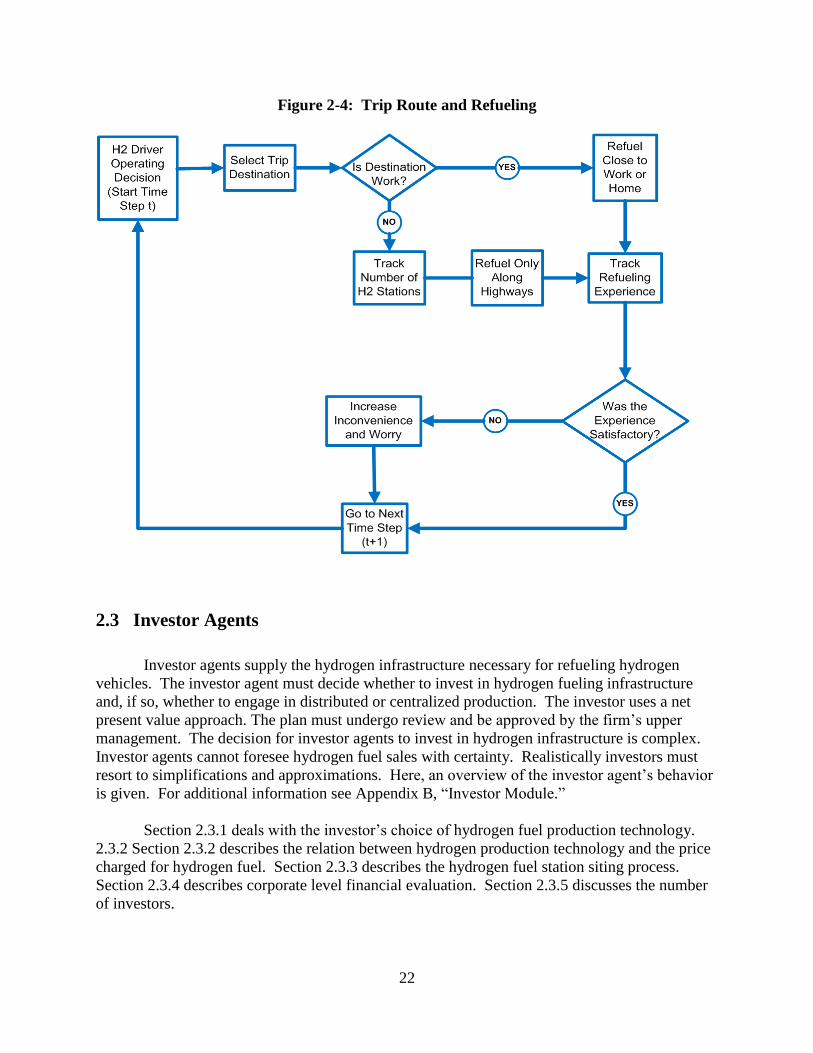
2.2.3 Vehicle Refueling
Refueling behavior influences the driver utility function by increasing or decreasing the
inconvenience and worry parameters of the driver utility function. Calculating worry and
inconvenience requires knowing where agents travel (travel behavior), and how they prefer to
refuel (refueling behavior). The driver agent’s trip route is important in determining refueling
behavior, as described in Figure 2-4. The figure indicates how refueling prospects differ
between work and non-work trips, and illustrates the evaluation of refueling in each quarter.
Driver agents evaluate when and where to refuel based on three potential fueling
conditions: willing-to-refuel level; want-to-refuel level; and desperate-to-refuel level. Whenever
driver agents stop to refuel, they top off their fuel tanks so that the fuel purchased is equal to the
maximum tank capacity minus current fuel level. The outcome of the refueling decision process
will influence whether driver agents decide to purchase hydrogen vehicles, and will also affect
hydrogen fuel sales. The outcome may change from period to period as more hydrogen fueling
stations are sited during a simulation. For an in depth description of driver agent trip routes and
the refueling decision process, see Section A.3 of Appendix A, ―Refueling.‖
22
Figure 2-4: Trip Route and Refueling
2.3 Investor Agents
Investor agents supply the hydrogen infrastructure necessary for refueling hydrogen
vehicles. The investor agent must decide whether to invest in hydrogen fueling infrastructure
and, if so, whether to engage in distributed or centralized production. The investor uses a net
present value approach. The plan must undergo review and be approved by the firm’s upper
management. The decision for investor agents to invest in hydrogen infrastructure is complex.
Investor agents cannot foresee hydrogen fuel sales with certainty. Realistically investors must
resort to simplifications and approximations. Here, an overview of the investor agent’s behavior
is given. For additional information see Appendix B, ―Investor Module.‖
Section 2.3.1 deals with the investor’s choice of hydrogen fuel production technology.
2.3.2 Section 2.3.2 describes the relation between hydrogen production technology and the price
charged for hydrogen fuel. Section 2.3.3 describes the hydrogen fuel station siting process.
Section 2.3.4 describes corporate level financial evaluation. Section 2.3.5 discusses the number
of investors.

23
2.3.1 Hydrogen Fuel Production Technologies
The major hydrogen production technologies considered in this study are distributed and
centralized stream methane reforming. Steam methane reforming is used because it appears to
be the most likely hydrogen production technology for the model area centered on the Los
Angeles metropolitan area. H2A models indicate that SMR is less expensive than either
electrolysis or coal gasification. It is unlikely that sufficient volumes of biomass would be
available to produce all the hydrogen needed in the latter years of the simulation via biomass
gasification.4
Steam methane reforming (SMR) consists of heating methane to 700o - 1,100
o C which
separates it into carbon monoxide and hydrogen.5 With distributed SMR production, small
reforming units are located at each refueling site. With centralized SMR production, a large
reformer serves many refueling sites by pipeline or truck delivery.
The investor faces a choice between building distributed SMR stations, and building
centralized plants along with a pipeline infrastructure for delivery of fuel. To make the choice
between the two technologies, the investor compares the levelized cost of producing hydrogen
using the centralized technology with the levelized cost using distributed stations. The shift to
centralized technology, once made, is never undone.
2.3.1.1 Distributed Production
Distributed production is characterized by location of production and dispensing
infrastructure at the same site. Distributed steam methane reformers (SMR) use natural gas to
produce hydrogen fuel with limited storage on-site. While there are a number of possible sizes
of distributed reformers, analysis with DOE’s H2A cost model suggests that a 1,500-kg/day
reformer with an effective capacity of 85.2% is the most cost-effective of the sizes in the array of
available sizes. The full capital cost of a 1,500-kg/day SMR facility is $4.8 million in 2009
4 Examination of the land in a 50-mile radius around the city of Los Angeles reveals only 515,000 usable acres for biomass
production: U.S. Department of Agriculture and the National Agricultural Statistics, 2007 Census of Agriculture – County
Data – California, Volume 1, ―Table 8: Farms, land in Farms, Value of Land and Buildings, and Land Use: 2007 and 2002,‖
available at http://www.agcensus.usda.gov/Publications/2007/Full_Report/Volume_1,_Chapter_2_
County_Level/California/index.asp (accessed March 29, 2010). 7.6 million hydrogen vehicles travelling 12,150 miles per year
with a fuel efficiency of 19.9 grams of hydrogen per mile would require biomass production levels of roughly 47 tons per acre
of the available acreage, well above the range of possible production levels for switchgrass and poplar reported in Robin L.
Graham, Erik Lichtenberg, Vernon O. Roningen, Hossein Shapouri, and Marie E. Walsh, The Economics of Biomass
Production in the United States, Oak Ridge National Laboratory, 1995, ―Table 1: Potential Biomass Crops, Suitable Acreages,
and Average Yields,‖ available at http://bioenergy.ornl.gov/papers/bioam95/graham3.html (accessed March 29, 2010). The
biomass-to-hydrogen conversion rate was taken from the Department of Energy’s H2A model: U.S. Department of Energy,
―Advanced (2010-2020) Hydrogen from Biomass via Gasification and Catalytic Steam Reforming,‖ Department of Energy
Hydrogen Program, January 4, 2005, http://www.hydrogen.energy.gov/h2a_prod_studies.html (accessed December 3, 2007). 5 U.S. Department of Energy, ―Hydrogen Production, Natural Gas Reforming,‖
http://www1.eere.energy.gov/hydrogenandfuelcells/production/natural_gas.html, accessed February 2010.

24
dollars.6 The smaller 100-kg/day SMR facility’s capital cost is $593 thousand, also in 2009
dollars.7
Figure 2-5 shows a comparison of the average cost of producing hydrogen using several
100-kg/day stations or one 1,500-kg/day station. The chopped cost curve refers to 100-kg/day
stations, and the smooth curve refers to one 1,500-kg/day station. As the number of hydrogen
vehicles increases, the average cost of producing hydrogen first declines due to increased
capacity utilization. When the existing 100-kg/day stations reach capacity, a new station needs
to be added to meet additional demand as shown by the spikes in the average cost curve. Low
initial capacity utilization associated with new stations leads to discrete jumps in the average
cost. With 400 vehicles to serve, a 1,500-kg/day station becomes more cost-effective, and its
advantage grows with additional vehicles.
The following conclusions can be drawn:
The lowest cost that can be realized with 100-kg/day stations is $9.21 per kg, whereas the
lowest cost that can be realized with a 1,500-kg/day station is $3.16 per kg.
Larger fuel stations become the least costly alternative at relatively low levels of demand.
A 1,500 kg/day station can serve 1,995 vehicles. A 100-kg/day station is sufficient to
serve 133 drivers [100 kg/day times 85.2% capacity utilization divided by (12,150 miles /
365 days) times 52 miles/kg]. Therefore the first three 100-kg/day stations can serve 399
vehicles; to serve the 400th
vehicle, a fourth 100-kg/day station would have to be
established. From Figure 2-5, even if there are only 400 vehicles to be served it is less
expensive to build the bigger plant and operate it initially at low capacity rather than
build four 100-kg/day plants, one at a time.
In view of these results, this study assumes that investors considering distributed
production in the model area will use 1,500-kg/day stations.
6 U.S. Department of Energy, ―Future (2025) Natural Gas Steam Reformer (SMR) at Forecourt 1500 kg/day,‖ Department of
Energy Hydrogen Program, May 27, 2008. http://www.hydrogen.energy.gov/h2a_prod_studies.html (accessed February 17,
2009). 7 U.S. Department of Energy, ―Forecourt Hydrogen Production,‖ ―h2a_forecourt_smr_100kgperday_ current_final.xls,‖
Department of Energy Hydrogen Program, October 14, 2004.
http://www.hydrogen.energy.gov/h2a_prod_studies.html (accessed December 2005).

25
Figure 2-5: Comparison of Average Cost of Producing Hydrogen using a 1,500 kg/day
SMR Station vs. 100-kg/day SMR Stations
-
2
4
6
8
10
12
14
16
18
20
0 100 200 300 400 500 600 700 800 900 1000 1100 1200 1300 1400 1500 1600 1700 1800 1900
Hydrogen Vehicles on Road
$ /
Kg
1500 kg/day station
100 kg/day stations
Source: Calculations made with H2A models.8 Costs are expressed in 2009 dollars.
2.3.1.2 Centralized Production
Centralized SMR production facilities are large plants capable of producing hydrogen at a
lower cost per kg than 1,500-kg/day on-site reformers. However, centralized plants rely on a
pipeline or truck delivery system which moves the hydrogen from the plant to fueling forecourts,
which also has to be located by the investor. In view of the cost of this added distribution
infrastructure, a large volume of sales must be made to bring average total cost of production
plus delivery to a level comparable to the cost of distributed production. From H2A, centralized
production plants have a nameplate capacity of about 380,000 kg/day, and the associated
forecourts have a nameplate capacity of 1,500 kg/day, with effective capacity of 85.2%, the same
as distributed fueling stations.
Using H2A cost numbers, a centralized plant requires $275 million in capital costs spread
over 4 years plus $10 million in recurring annual costs during operation. The accompanying
8 U.S. Department of Energy, ―Future Forecourt Hydrogen Production from Natural Gas (100 kg per day),‖ October 14, 2004,
and ―Future Forecourt Hydrogen Production from Natural Gas (1,500 kg per day),‖ October 14, 2004, available at
http://www.hydrogen.energy.gov/h2a_prod_studies.html. (Accessed December 2005.) Default assumptions. Costs have been
converted to 2009 dollars.

26
delivery and dispensing infrastructure requires $13 billion in capital costs9 and provides a
transmission pipeline, two urban trunk lines and service pipelines to the fueling stations,
geologic storage, compressors and dispensing stations. Truck distribution was found to be more
expensive than pipeline distribution. Not considered here are problems of securing rights-of-way
for new pipeline in urban areas and problems of traffic congestion and gas pressures beyond
contemporary standards for truck transportation.
The cost per kilogram of centralized hydrogen production is high if it is introduced in
early years of the hydrogen transition when there is not yet sufficient volume to cover its fixed
costs, as shown in Panel (1) of Figure 2-6. The levelized cost necessary to recover fixed costs
over the life of the project declines as the year of introduction of centralized production is
delayed. Centralized production is begun in the year when volume has become sufficient for its
levelized cost to fall below the cost of distributed production. In the illustrative example
presented here, the cost of distributed production is $3.50 per kg. As shown in Panel (2) the
levelized cost of centralized production falls to $3.50 per kg by the seventh year, which is the
year of switchover from distributed to centralized production. Panel (3) shows that as the rate of
adoption of hydrogen vehicles increases, an earlier switchover to centralized production would
occur due to the increased fuel demand in early years. Panel (4) shows the effect that higher
prices of distributed production would have in speeding up entry of centralized production, such
as might be brought about by a carbon tax on distributed production. Since carbon capture and
sequestration is impractical with distributed production, its hydrogen would be taxed as much as
gasoline, if not slightly more. Carbon capture and sequestration are possible with centralized
production, and any carbon tax would be substantially lower on hydrogen provided in such a
manner than on hydrogen produced at distributed stations or on gasoline.
9 U.S. Department of Energy, ―Future Central Hydrogen Production from Natural Gas with CO2 Sequestration version 2.1.1,‖
May 27, 2008, http://www.hydrogen.energy.gov/h2a_prod_studies.html. (Accessed August 2009). Default assumptions. Costs
have been converted to 2009 dollars.

27
Figure 2-6: Factors Affecting Entry of Centralized Production
2.3.2 Price Charged for Hydrogen Fuel
The investor charges a price for fuel that is equal to the average cost of producing
hydrogen. It is assumed that this behavior is brought about by threat of entry by new suppliers or
of regulation if monopoly prices are charged, Section B.1 of Appendix B, ―Price Charged for
Hydrogen Fuel,‖ provides the mathematical formula for average cost used to calculate the price
of hydrogen fuel in the model.
2.3.3 Station Siting
The investor makes decisions about siting stations at the beginning of each simulation
year, starting at the second year. In the first year of a simulation, only seed stations exist. At the
beginning of the second year, and of each subsequent year, the investor creates a station siting
plan for the year and has the opportunity to site as many stations as desired at each of the
possible fueling station locations.
(1) Costs of Unused Centralized Capacity Are
Raised by Early Entry of Centralized
Production
$0.00
$2.00
$4.00
$6.00
$8.00
$10.00
$12.00
$14.00
$16.00
1 3 5 7 9 11 13 15 17 19 21 23 25 27 29 31 33 35 37
Year
Yearl
y C
ost
per
Kg
3
8
13
18
23
28
Year of
Centralized Entry
(2) Levelized Price Needed to Repay Centralized
Costs Competes with Distributed Price
$2.00
$3.00
$4.00
$5.00
$6.00
$7.00
$8.00
1 3 5 7 9 11 13 15 17 19 21 23 25 27 29 31
Year of Centralized Entry
Levelized o
f C
ost
Per
Kg
Centralized Cost if Entryfor Year Indicated
Distributed Cost3:
$4.23 8:
$3.4
8
13:
$3.25
Actual Year
Of Entry
18:
$3.19 23:
$3.18
28:
$3.19
(3) Year of Centralized Entry is Lowered By
More Rapid Hydrogen Vehicle Adoption
$2.00
$3.00
$4.00
$5.00
$6.00
$7.00
$8.00
1 3 5 7 9 11 13 15 17 19 21 23 25 27 29 31
Year of Centralized Entry
Levelized
Co
st
Per
Kg
Very Slow Adoption
Slow Adoption
Benchmark Adoption
Rapid Adoption
Very Rapid Adoption
Distributed Cost
-----<$3.19
1471014$3.50
11126$5.50
11111>$7.56
Very
RapidRapidBenchmarkSlow
Very
Slow
Vehicle Adoption Rate
Distributed
Price
-----<$3.19
1471014$3.50
11126$5.50
11111>$7.56
Very
RapidRapidBenchmarkSlow
Very
Slow
Vehicle Adoption Rate
Distributed
Price
(4) Year of Centralized Entry is Lowered
By Higher Distributed Price

28
Establishing a new station can affect future demand at other locations. This happens
when a station is established at a location where no station existed previously and is able to
attract some of the drivers who would otherwise refuel at nearby locations. If the investor does
decide to add another station, the previous estimates of likely sales at all the locations near this
station are reduced by the expected diversion of sales from these locations to the new station.
Section 2.3.3.1 describes the possible station locations within the model area. Section
2.3.3.2 describes the steps in the station siting decision. Further details and equations used in the
station siting procedure are provided in Section B.2 of Appendix B, ―Station Siting.‖
2.3.3.1 Possible Station Locations in Model Area
The model area is divided into 5,000 1x1-mile cells. While there are 2,500 cells where
driver agents may reside, the investor agent is restricted to siting stations in 156 cells located at
major highway intersections and at the midpoints of highway segments. These highway
intersections are indicated by the yellow dots in Figure 2-7. Each of these cells may have as
many stations as the investor chooses to site there.
Figure 2-7: Map of Potential Station Locations
2.3.3.2 Station Siting Steps
In the first year of the simulation, it is assumed that the only stations are seed stations.
Investor agents make station siting decisions from the second year onward. An overview of the
process is shown in Figure 2-8.

29
Figure 2-8: Overview of Investor Station Siting Process
The investor takes the following steps to decide whether to add another station to the
existing set of stations:
1. Estimate base sales for each possible location using observed sales for locations with
existing stations and using a regression of sales on traffic counts to estimate what sales
would be if a station were added at a location where none exists, allowing for diversion
of sales from existing stations if a new station is added. See Appendix B, Section
B.2.1.1, ―Unadjusted Sales at a Location‖ and Section B.2.1.2, ―Adjustments for Sales to
Stations Planned but Not Yet Operational,‖ for additional detailed information.
2. Estimate likely future sales at each possible location using a logistic growth function.
See Appendix B, Section B.2.1.3, ―Estimation of the Growth Parameter,‖ and Section
B.2.1.4, ―Estimating Future Sales at a Location Using a Logistic Growth Function,‖ for
details.
3. Using the estimate of likely future sales at each location, calculate the net present value
(NPV) of a new station at each location. See Appendix B, Section B.2.2.1, ―Net Present
Value (NPV) Calculations,‖ for details.

30
4. Rank locations according to the increase in NPV in Step 3. See Appendix B, Section
B.2.2.2, ―Ranking of Locations,‖ for details.
5. For a proposed new station at the highest-ranked location in the city, make the following
NPV calculations using the formulas in Appendix B, Section B.2.2.1, ―Net Present Value
(NPV) Calculations.‖
Default NPV: Calculate the NPV of the investor’s existing set of stations without the
proposed new station.
NPV with the proposed station: Calculate the NPV of the investor’s set of stations if
the proposed station is sited in the current year.
NPV with waiting: Calculate the NPV of the station set under the assumption that the
proposed station is sited not in the current year but in the following year.
6. Compare the NPV with the proposed station to the default NPV and to the NPV with
waiting. See Appendix B, Section B.2.2.3, ―Net Present Value (NPV) Rule for Station
Siting,‖ for details.
If the NPV with the proposed station exceeds both the default NPV and the NPV of
waiting, then it is profitable to site the station in the current year. The investor sites
the proposed station, and repeats Step 5 to see if any additional stations should be
sited at the same location in the current year.
If the NPV with the proposed station is less than either the default NPV or the NPV
with waiting then the investor decides not to site the proposed station.
7. Propose a new station at the next best location, and loop back to Step 5.
8. If there is no next best location because a new station has been proposed and rejected at
all 156 locations, then the station siting plan is complete for the current year.
2.3.4 Financial Evaluation of the Investment Plan
Financial evaluation of plans for undertaking infrastructure investments occurs at two
levels: evaluation by division staff and final decisions by upper management.
2.3.4.1 Staff Evaluation
The initial evaluation is conducted by corporate division staff, following textbook
principles along the lines of the NPV calculations described above. When the evaluation is

31
completed, the assessment is sent to upper management where investment decisions will be
made.
2.3.4.2 Upper Management Evaluation
Corporate executives make use of staff evaluations of potential investments but do not
regularly follow them exactly. Upper management may exhibit extremes of risk aversion or risk
tolerance. Using a wider range of discount rates than the division staff do, upper management
can accept or reverse division staff recommendations.
Business experience is replete with highly successful investments based on shrewd and/or
lucky estimates that far outstripped the rest of the market, as well as those of the opposite kind
resulting in large losses. This study investigates the possible role of these kinds of decisions in
influencing the provision of hydrogen infrastructure.
Typically, the division staff forwards potential investments that pass minimum financial
requirements to upper management. Upper management then takes additional considerations
into account that are outside the scope of the division staff, such as overall company goals, and
shareholder and lender perceptions. Upper management often has access to separate departments
outside the division staff that will assist them in their analysis, with titles such as Strategic
Planning and Investor Relations.
Figure 2-9 illustrates the structure of corporate decision-making. Multiple parties are
often involved in project investment decision making. These include: 1) the division staff, 2)
shareholders, 3) lending institutions, and 4) upper management. Figure 2-9 suggests that each
party has a role with separate objectives. The division is likely to seek funding for any profitable
projects that come to its attention. Upper management evaluates the projects proposed by
division staff. Upper management also communicates with the shareholders and is aware of the
available company resources, information on which division staff may not have direct
knowledge.

32
Figure 2-9: Role of Upper Management in Corporate Decision-Making
Most companies have limited funding available for new projects, resulting in some
profitable projects not being selected by a company. Other projects may be highly profitable but
small and short-lived. Still others may have lower profitability but be large and sustainable, with
the potential to provide cash for other projects in the future. Depending on the company’s goals,
upper management may find the larger, less profitable project to be a better fit for the company.
Upper management is typically sensitive to the funding providers’ opinions of the company. If
the company takes on a large project that its primary lender views as risky, the company may
find its debt costs rising the following year. Management wants to be confident that the
company is investing in projects that align with its shareholders’ interests and long-term goals.
Faced with these challenges, upper management chooses projects for inclusion in the
investment portfolio, giving attention to such indicators as return on investment, profitability,
and growth. A variety of financial metrics can be used to evaluate a project. This study focuses
on the commonly used metrics of discount rate, projected growth rate, and planning horizon. By
performing sensitivity analyses on these variables, the model can evaluate the effect of upper
management on the rate of vehicle adoption and whether ultimate adoption is affected. Because
the individual company decision process can vary even within an industry, different cases need
to be considered.
Responses by upper management may include:
1. Adjusting the discount rate to reflect the specific perceived risk level of a hydrogen
investment.
2. Adjusting the level of optimism or pessimism to reflect personal views about a new
market.
Upper Management
Shareholders
Upper Management Communicates
Via Announcements & Reports
Shareholders Communicate Via
Share Price by Buying or Selling Stock
Division 1 Division 2 Division 3
Pro
ject 1
Upper Management Will
Stringently & Skeptically
Evaluate the Projects to
Determine Funding
Company Funding
Resources -Retained Earnings
-Private Debt
-Public Debt
-Equity
Pro
ject 2
Pro
ject 3
Pro
ject 4
Pro
ject 5
Pro
ject 6
Pro
ject 7
33
3. Adjusting the rapidity of learning to reflect views about a new market.
4. Adjusting the planning horizon used to reflect concerns about short-term shareholder
opinion.
5. Adjusting capital availability to reflect a desire or need to keep the corporation’s
leverage level below a particular point.
Each of these responses is considered below:
1. Discount rate. Some upper management groups are conservative and others are more
risk tolerant. The discount rate used for an investor’s profit calculation represents the profit
level, or rate of return, required by the investor for the project to be attractive. In the division
staff scenario, rates of return are assumed that are reasonable and likely. However, what if the
investor has an upper management that is highly risk-tolerant or risk-averse? In the highly risk-
tolerant case upper management would pursue a project without being compensated adequately
for risk; this would correspond to use of a low discount rate. The opposite is true in the risk-
averse case: an investor would require an unusually high return for the risk level, corresponding
to a high discount rate. To illustrate the potential effects of an upper management intercession of
this type, additional scenarios would need to be investigated in which an investor uses more
extreme discount rates than used in the division staff scenarios.
2. Optimism or pessimism. The upper management of a company may find that it
disagrees with the current beliefs of its division staff. Without any substantive market data, an
investor selects an initial growth rate believed to be the growth rate of hydrogen fuel sales. This
rate is adjusted over time as the investor learns. Upper management may disagree with the
division staff’s initial growth projections and exhibit greater optimism or pessimism than a
purely financial view of the data would suggest. Optimism or pessimism at the division staff
level can be represented by a high or low value for the initial growth rate applicable to expected
hydrogen sales.
3. Rapidity of learning. Should the upper management disagree with its staff, it is likely
that even if conflicting data were to appear, upper management may still be skeptical of the
results. For this situation, the growth weights are altered in the learning calculation, as described
in Section B.2.1.3 of Appendix B, ―Estimation of the Growth Parameter,‖ to shift the basis of
upper management’s current beliefs toward either its previous beliefs or its latest observations.
If upper management places greater weight on the previous period’s information than on that of
the current period, this has the effect of creating a ―stubborn‖ investor, reflecting the possibility
of upper management relying on its first assessment about the market for a somewhat longer
period of time. By slowing the rapidity of learning the case can be simulated in which upper
management disagrees with the market data coming in and is slower to react to actual results.
This may also reflect considerations of upper management’s view of longer-term trends in the
specific business, the economy, or the policy environment that are not accounted for in the
current market response.

34
4. Planning horizon. Often upper management feels pressure to invest in projects that
will reward the shareholders with returns more quickly than others. This can cause the upper
management of some corporations to over-value short-term profits. Despite the longevity of the
hydrogen infrastructure, it is possible that upper management will look at a shorter time horizon
to make sure the shareholders receive a quick return on investment. In these cases upper
management is interested in knowing if the investment can pay for itself in a certain timeframe
ignoring the cost of capital. If the project restricts capital for too long, upper management may
be hesitant to invest.
5. Restrict capital. Capital budgeting is an important component of upper management’s
decision-making responsibilities. Some companies will have greater ability to fund a large
investment in hydrogen than will others. Those companies with large existing investments may
find resistance from corporate lenders and shareholders to providing them with additional
inexpensive liquidity. For the right profit level, capital can usually be found for even the most
leveraged company. However in the early stages of an unproven market, capital may be
restricted for companies with existing high levels of leverage.
2.3.5 Number of Investors
Most of the simulations reported in this study have been for a single investor agent. If a
single investor acted as a monopolist to substantially raise the price of hydrogen, the number of
investors might have more important effect in acting to bid down the price of hydrogen.
However, as noted above in Section 2.3.2, ―Price Charged for Hydrogen Fuel,‖ threats of
potential competition and of regulation are assumed to keep the price of hydrogen close to its
average cost of production.
The methodological complications for the multiple investor case are described in Section
B.3, ―Number of Investors,‖ in Appendix B. Results of a sensitivity study showing that the
number of investors has little impact on the sales of hydrogen vehicles are presented in the text
below in Section 3.3.6, ―Number of Investors.‖

35
PART THREE: SENSITIVITY TO MODEL PARAMETERS
In order to understand the effects of driver and investor agents on the rapidity of adoption
of hydrogen vehicles, sensitivity analyses were conducted on selected parameters used in the
model. As discussed in Part Two, the model contains 130 parameters which consist of 92 cost
parameters from DOE’s H2A model10
, 17 driver behavior parameters, 10 investor behavior
parameters, and 11 price and policy variables.
The sensitivity analyses were conducted in relation to a benchmark case. The purpose of
this study is to examine hydrogen vehicle growth and the provision of hydrogen infrastructure
once hydrogen vehicles become competitive in the marketplace. The benchmark case provides
an example of a set of prices for vehicles, as well as fuels for hydrogen and non-hydrogen
vehicles that would result in cost competitiveness and allow a take-off. It is to be emphasized
that this study does not attempt to predict the year when the required cost competitiveness will be
achieved.
The results presented in this section are for the following three parameters pertaining to
driver agent behavior: driver familiarity with hydrogen vehicles, the bandwagon effect or the
impact of drivers who have already bought a hydrogen vehicle on drivers who have not bought
one yet, and taste for greenness or driver willingness to pay a premium for an environmentally
friendly vehicle.
Results are also presented for six parameters pertaining to investor behavior: staff
discount rate, upper management discount rate, rapidity of learning, expectation of growth,
demand estimation method, and number of investors. Effects are explored of the use of
approximative decision making by investors on whether the same penetration is ultimately
reached as with exact optimization and how the rapidity of adoption is affected.
The benchmark case is described in Section 3.1. Sensitivity scenarios for driver
parameters are presented in Section 3.2. Sensitivity scenarios for investor parameters are
presented in Section 3.3. Effects of approximative decision-making are examined in Section 3.4.
3.1 Benchmark Case
The benchmark case represents a 40 year scenario where hydrogen vehicles and fuel
become competitive with traditional vehicles. Section 3.1.1 presents values for the major driver
and investor agent parameters used in the benchmark case. Section 3.1.2 shows the results of the
benchmark scenario for hydrogen vehicles sales market penetration. Section 3.1.3 shows the
results for the market penetration of the stock of hydrogen vehicles. Section 3.1.4 presents the
growth of the number of stations under the benchmark case. Section 3.1.5 provides an overview
10 U.S. Department of Energy, ―Future (2025) Natural Gas Steam Reformer (SMR) at Forecourt 1500 kg/day,‖ Department of
Energy Hydrogen Program, May 27, 2008. http://www.hydrogen.energy.gov/h2a_prod_studies.html (accessed February 17,
2009). All cost figures in the present report have been updated to 2009 dollars.

36
of the distribution of fuel stations within the model area at selected years. Section 3.1.6 presents
estimates of investor agent cash flows.
3.1.1 Parameter Values for the Benchmark Case
Values for the main driver agent and investor agent parameters used in the benchmark
scenario are shown in Table 3-1. Among the driver agent parameters, the disadvantage due to
limited familiarity is the additional amount a driver without any knowledge of the hydrogen
vehicle would have to be paid to buy the vehicle. The parameter for the bandwagon effect is a
coefficient of the proportion of drivers who have already adopted hydrogen vehicles. Greenness
central tendency is the premium the median driver is willing to pay for an environmentally
friendly vehicle. Greenness dispersion is a measure of how the degree of preference for
greenness varies among the population of drivers.
The benchmark values of the investor agent parameters are taken from DOE’s H2A
model.11
The fueling station capital cost is based on a 1,500-kg/day steam methane reforming
station. Fixed operations and maintenance (O&M) costs are incurred annually and do not vary
with the volume of hydrogen produced. The salvage value is the excess of terminal-period asset
value of a station over decommissioning costs. The investor discount rate is the interest rate at
which future income and costs are discounted. The hydrogen selling price equals the average
cost of hydrogen production as described above in Section 2.3.2, ―Price Received for Hydrogen
Fuel.‖ The fuel station operating capacity is the average annual daily hydrogen production level,
allowing for maintenance down time and statistically anticipated outages.
11 Ibid.

37
Table 3-1: Parameter Values for the Benchmark Case
Parameter Value
Driver Agent Parameters
Disadvantage Due to Limited Familiaritya,f
$12,000
Bandwagon Effect Coefficient a 0.1
Bandwagon Effect Dispersion a 2.2
Greenness Central Tendencyb,f
$250
Greenness Dispersionb 10
Investor Agent Parameters
Fueling Station Capital Costc,f
$4,806,357
Fueling Station Fixed O&M Costsc,f
$236,598
Fueling Station Salvage Valuec 0
Investor Discount Rated 10%
Hydrogen Selling Pricee,f
$3.63/kg
Fueling Station Operating Capacityc 1,278 kg/day
a
For additional discussion see Section A.2.3 in Appendix A, ―Disadvantage Due to Limited
Familiarity and Bandwagon Coefficient, F
jtP and qj.‖
b For additional discussion see Section A.2.4 in Appendix A, ―Greenness, Tj.‖
c Station nameplate capacity of 1,500 kg/day from DOE H2A model.
d DOE H2A model.
e For additional discussion see Section B.1 in Appendix B, ―Price Charged for Hydrogen Fuel.‖
f In 2009 dollars.
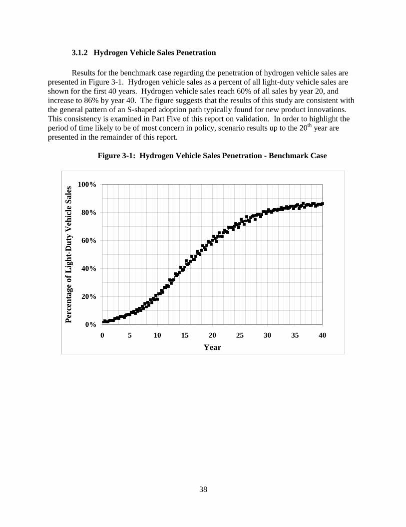
38
3.1.2 Hydrogen Vehicle Sales Penetration
Results for the benchmark case regarding the penetration of hydrogen vehicle sales are
presented in Figure 3-1. Hydrogen vehicle sales as a percent of all light-duty vehicle sales are
shown for the first 40 years. Hydrogen vehicle sales reach 60% of all sales by year 20, and
increase to 86% by year 40. The figure suggests that the results of this study are consistent with
the general pattern of an S-shaped adoption path typically found for new product innovations.
This consistency is examined in Part Five of this report on validation. In order to highlight the
period of time likely to be of most concern in policy, scenario results up to the 20th
year are
presented in the remainder of this report.
Figure 3-1: Hydrogen Vehicle Sales Penetration - Benchmark Case
0%
20%
40%
60%
80%
100%
0 5 10 15 20 25 30 35 40
Year
Per
cen
tag
e o
f L
igh
t-D
uty
Veh
icle
Sa
les

39
3.1.3 Hydrogen Vehicle Stock Penetration
In Figure 3-2, the stock of hydrogen vehicles as a percentage of the total stock of light-
duty vehicles is shown for the first 40 years using the benchmark case. The stock penetration is
lower than the sales penetration at any given time, as a vehicle lasts for many years and only a
fraction of the total vehicle stock is replaced in any one year. For instance, the stock penetration
is 25% by the 20th
year, whereas sales penetration is 60%. By the 40th
year, the stock
penetration is 77%, while the sales penetration is 86%.
Figure 3-2: Stock of Hydrogen Vehicles as Percent of Total Light-Duty Vehicles -
Benchmark Case
0%
20%
40%
60%
80%
100%
0 5 10 15 20 25 30 35 40
Year
Per
cen
tag
e o
f L
igh
t-D
uty
Veh
icle
Sto
ck
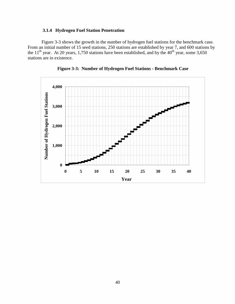
40
3.1.4 Hydrogen Fuel Station Penetration
Figure 3-3 shows the growth in the number of hydrogen fuel stations for the benchmark case.
From an initial number of 15 seed stations, 250 stations are established by year 7, and 600 stations by
the 11th
year. At 20 years, 1,750 stations have been established, and by the 40th
year, some 3,650
stations are in existence.
Figure 3-3: Number of Hydrogen Fuel Stations - Benchmark Case
0
1,000
2,000
3,000
4,000
0 5 10 15 20 25 30 35 40
Year
Nu
mb
er o
f H
yd
rog
en F
uel
Sta
tio
ns

41
3.1.5 Location of Fuel Stations
Figure 3-4 illustrates how the model chooses the location of stations over time. The
illustrations shown are for years 5, 10, 20, and 40.
Figure 3-4: Illustration of Hydrogen Fuel Station Growth
Hydrogen Fuel Stations in Model Area: Year 5 Hydrogen Fuel Stations in Model Area: Year 10
Hydrogen Fuel Stations in Model Area: Year 20 Hydrogen Fuel Stations in Model Area: Year 40
Note: The model area is a rectangular 100 mile x 50 mile area centered on Los Angeles, California. Station locations may
represent multiple stations.
3.1.6 Investor Agent Cumulative Cash Flows
Many financial measurements for investors can be calculated. As an example, Figure 3-5
shows cumulative cash flows for the investor during the first twenty years. The green line shows
the undiscounted cash flows. The line reaches its lowest point in year 16, which shows that for

42
the first 16 years, any profits from the existing stations would be exceeded by capital outlays
required for the new stations that the investor decides to site. An implication is that the investor
in this benchmark scenario would require net cash infusions during the first 16 years.
The blue line presents the discounted cash flow using a 10% annual discount rate. In this
scenario, 30 years are required before the project earns a positive net return.
Figure 3-5: Investor Portfolio Valuation under the Benchmark Scenario
-1,400
-1,200
-1,000
-800
-600
-400
-200
0
200
400
600
0 5 10 15 20 25 30 35 40
Year
Dis
cou
nte
d (
$m
)
-5,000
0
5,000
10,000
15,000
20,000
25,000
Un
dis
cou
nte
d (
$m
)
Discounted Cumulative Cash Flow
Undiscounted Cumulative Cash Flow
In 2009 dollars.
3.2 Driver Sensitivity Scenarios
This section presents the results of sensitivity scenarios for three major driver behavior
parameters. Section 3.2.1 examines sensitivity to driver familiarity with a hydrogen vehicle.
Section 3.2.2 presents sensitivity to the bandwagon effect. Section 3.2.3 gives sensitivity results
for a driver’s taste for greenness. Section 3.2.4 summarizes the results of the driver sensitivity
scenarios.
3.2.1 Driver Familiarity
At the beginning of a simulation, driver agents are unfamiliar with hydrogen vehicle
technology. This unfamiliarity depresses the amount they are willing to pay for a hydrogen
vehicle. The magnitude of this value, measured in dollars, is the disadvantage due to limited

43
familiarity. Stated alternatively, the disadvantage due to limited familiarity is the amount of
money that the average buyer would need to be paid to buy a hydrogen vehicle, given no
knowledge about it. The value of the disadvantage due to limited familiarity used in the
benchmark case is $12,000. This amount is roughly the difference between the manufacturer’s
suggested retail price for the average light-duty vehicle (approximately $23,000) and the least
costly light-duty vehicle (approximately $11,000).12
In the sensitivity analyses, the difference
between the average vehicle price and the average price of small vehicles such as the Chevrolet
Aveo and the Honda Fit, is closer to $8,000, which is the lower bound. The average price of a
light-duty vehicle, $23,000, is used as the upper bound.
As shown in Figure 3-6, sales penetration grows as driver familiarity increases, reaching
79% by the 20th
year, compared to 60% in the benchmark scenario. In the scenario where driver
agents are less familiar with hydrogen vehicles, adoption is substantially slowed, with sales
penetration reaching only 24% in the 20th
year.
Figure 3-6: The Effect of Disadvantage Due to Limited Familiarity
on Hydrogen Vehicle Sales Growth
0%
20%
40%
60%
80%
100%
0 5 10 15 20
Year
Per
cen
tag
e o
f L
igh
t-D
uty
Veh
icle
Sa
les Discount = $8,000
Discount = $12,000 (Benchmark)
Discount = $23,000
12 Ward’s Automotive Yearbook, 2009.
Disadvantage Due to Limited
Familiarity
Hydrogen Vehicle Sales Penetration
5 yr 10 yr 15 yr 20 yr
$8,000 (Agents have more familiarity) 20% 45% 66% 79%
$12,000 (Benchmark) 7% 18% 41% 60%
$23,000 (Agents have less familiarity) 1% 3% 9% 24%

44
3.2.2 Bandwagon Effect
The bandwagon effect parameter influences the hydrogen vehicle adoption rate by
affecting the driver’s familiarity with hydrogen vehicles. A driver agent’s disadvantage due to
unfamiliarity declines as the opportunity to observe the new technology in operation increases.
This effect has been observed universally in the adoption of new consumer durables and is a
major consideration in the behavior of the driver agents in this model.
For the scenario analyses, the strength of the bandwagon effect is varied using a central
tendency value. Each driver has a value for the strength of the bandwagon effect, which is
calibrated using a log normal distribution. The distribution of the population’s bandwagon
strengths has a central tendency value associated with it. When the central tendency value is
increased, the bandwagon effect becomes stronger for all drivers. When it is decreased, the
bandwagon effect becomes weaker for all drivers. In the benchmark case, the central tendency
value is 0.1, which means that the median driver’s familiarity will increase by 1% for every 10%
of other drivers who already own hydrogen vehicles.
A dispersion value, which controls the number of drivers at the high and low ends of the
distribution, is also included. The benchmark dispersion value is 2.2. This choice of benchmark
is calibrated to match the bandwagon effect of a selection of consumer durable goods to which
the adoption of hydrogen vehicles might be compared. The high and low magnitudes of the
bandwagon effect are calibrated to be similar to the adoption rates of air conditioning and color
television, which are products representative of high and low levels of bandwagon effect.13
As shown in Figure 3-7, hydrogen sales penetration grows more rapidly in the scenario
with the strong bandwagon effect, as drivers grow more familiar with the new technology more
rapidly. In addition, the effect is much stronger in early years than in later ones. After 10 years,
the slower-than-benchmark bandwagon effect scenario results in sales penetration of 10%, while
the faster-than-benchmark scenario results in sales penetration of 63%, compared to a benchmark
of 18%. After 20 years, sales penetration reaches 94% in the faster-than-benchmark scenario,
but only 27% in the slower-than-benchmark scenario.
13 Frank M. Bass, ―A New Product Growth Model for Consumer Durables,‖ Management Science, 15 (1969): 215-227 [
Reprinted in Management Science 50, No. 12 Supplement (2004): 1825-1832.]; Frank M. Bass, Trichy V. Krishnan, and
Dipak C. Jain, ―Why the Bass Model Fits without Decision Variables,‖ Marketing Science 13 (1994): 203-223; and Farrena
Sultan, John U. Farley, and Donald R. Lehmann, ―A Meta-Analysis of Applications of Diffusion Models,‖ Journal of
Marketing Research 27 (1990): 70-77.

45
Figure 3-7: Effect of Bandwagon Strength on Hydrogen Vehicle Sales Growth
0%
20%
40%
60%
80%
100%
0 5 10 15 20
Year
Per
cen
tag
e o
f L
igh
t-D
uty
Veh
icle
Sa
les Bandwagon Central Tendency = 0.30
Bandwagon Central Tendency = 0.10 (Benchmark)
Bandwagon Central Tendency = 0.05
3.2.3 Greenness
Each driver has a taste for greenness, which is represented by the additional amount of
money the driver would be willing to pay for the perceived environmental benefits of a hydrogen
vehicle. Similar to the bandwagon effect, the greenness values are log-normally distributed with
a central tendency and dispersions that measure the distribution of the taste for greenness in the
driver agent population. The minimum level of greenness is $0. Most drivers cluster at similar,
low values, with a minority of drivers having very high values. Scenarios were conducted on
both dispersion and central tendency.
The dispersion measure describes how diverse the drivers are. The larger the dispersion,
the more drivers have extreme tastes for greenness. If the central tendency value of greenness is
$250 and the dispersion measure is 10, as in the benchmark, then 68.3% of agents will have
greenness levels between $25 and $2,500. If the dispersion measure is 6, 68.3% of agents will
have greenness levels between $42 and $1,500.
Bandwagon Central Tendency Hydrogen Vehicle Sales Penetration
5 yr 10 yr 15 yr 20 yr
0.30 24% 63% 92% 94%
0.10 (Benchmark) 7% 18% 41% 60%
0.05 5% 10% 16% 27%

46
The choices of a central tendency value of $250 and a dispersion measure of 10 to define
the benchmark greenness distribution are based on evidence of willingness to pay for a green
vehicle observed among hybrid buyers and reported in stated-preference surveys.14
The high
value of the central tendency represents a 150% increase above the benchmark level, while the
low value is chosen to represent no median greenness effect. Because hybrid buyers provide an
imperfect example of greenness—they are also influenced by fuel savings, tax credits, and the
limited variety of hybrid vehicle models—and because people may not act exactly the way they
respond in stated preference surveys, there is uncertainty about the actual influence of greenness
on driver purchasing decisions. The sensitivity estimates attempt to reflect that uncertainty.
Results are shown in Figure 3-8 for sensitivity to greenness central tendency. If the
central tendency is $375 as opposed to the benchmark case of $250, penetration by the 20th
year
is 69% as compared to 60% in the benchmark case. If the central tendency is a low $1, sales
penetration by the 20th
year is only 17%.
14 Information on hybrid vehicles is taken from Matthew E. Kahn, ―Do Greens Drive Hummers or Hybrids? Environmental
Ideology as a Determinant of Consumer Choice,‖ Journal of Environmental Economics and Management 54 (2007): 129-145;
and Ward’s Automotive Yearbook, 2008. Stated preference sources are R. Graham, Comparing the Benefits and Impacts of
HEV Options (Palo Alto, Calif. EPRI, 2001), D. J. Santini and A. D. Vyas, Suggestions for a New Vehicle Choice Model
Simulating Advance Vehicles Introduction Decisions (AVID): Structure and Coefficients, Center for Transportation Analysis,
Argonne National Laboratory, 2005; and Melanie Tompkins, David Bunch, Danilo Santini, Mark Bradley, Anant Vyas, and
David Poyer, ―Determinants of Alternative Fuel Vehicle Choice in the Continental United States,‖ Transportation Research
Record: Journal of the Transportation Research Board 1641 (1998): 130-138. The benchmark central tendency and
dispersion used in the model are mean values calculated from data in these reports.
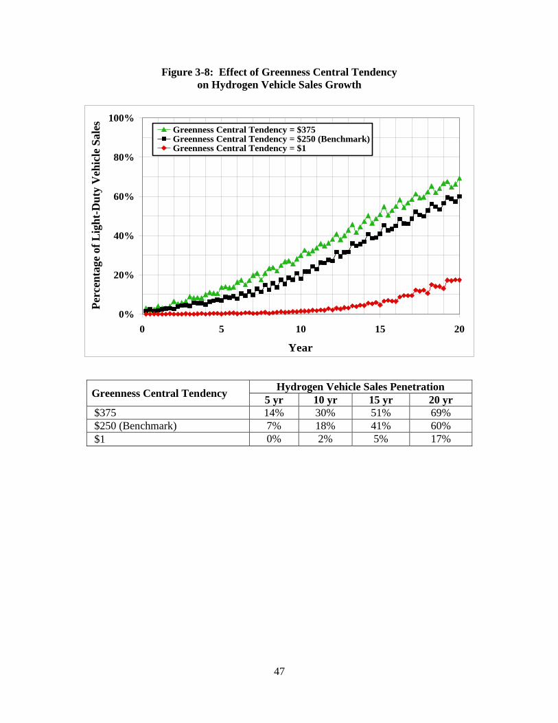
47
Figure 3-8: Effect of Greenness Central Tendency
on Hydrogen Vehicle Sales Growth
0%
20%
40%
60%
80%
100%
0 5 10 15 20
Year
Per
cen
tag
e o
f L
igh
t-D
uty
Veh
icle
Sa
les
Greenness Central Tendency = $375Greenness Central Tendency = $250 (Benchmark)Greenness Central Tendency = $1
Greenness Central Tendency Hydrogen Vehicle Sales Penetration
5 yr 10 yr 15 yr 20 yr
$375 14% 30% 51% 69%
$250 (Benchmark) 7% 18% 41% 60%
$1 0% 2% 5% 17%

48
Results are shown in Figure 3-9 for sensitivity to greenness dispersion. The range
considered is from a high dispersion value of 20 and a low value of 2, representing a larger
number of drivers with strong and weak tastes for greenness and a very small number of each,
respectively. In the high dispersion scenario, sales penetration by the 20th
year is 71%, 11
percentage points higher than in the benchmark scenario. In the low dispersion scenario, sales
penetration by the 20th
year reaches only 21%, 39 percentage points lower than in the
benchmark.
Figure 3-9: Effect of the Dispersion of Greenness
on Hydrogen Vehicle Sales Growth
0%
20%
40%
60%
80%
100%
0 5 10 15 20
Year
Per
cen
tag
e o
f L
igh
t-D
uty
Veh
icle
Sa
les Greenness Dispersion = 20
Greenness Dispersion = 10 (Benchmark)
Greenness Dispersion = 2
3.2.4 Conclusions on Model Sensitivity to Driver Behavior
As can be seen in the scenarios reported in this section, assumptions about driver agent
behavior have a significant effect on the results of the model. The strength of driver familiarity
has a large influence on hydrogen vehicle sales growth. A change in the disadvantage due to
Greenness Dispersion Value Hydrogen Vehicle Sales Penetration
5 yr 10 yr 15 yr 20 yr
20 15% 32% 54% 71%
10 (Benchmark) 7% 18% 41% 60%
2 0% 2% 6% 21%
49
limited familiarity creates an early change in sales that compounds over time. The level of driver
agent familiarity can substantially accelerate or delay the rate of hydrogen vehicle adoption, even
if hydrogen vehicles still dominate the market in the long-run. While the literature has much to
say on how to estimate the disadvantage due to limited familiarity, there are justifications for a
number of different values. The influence of the bandwagon effect on hydrogen vehicle sales
serves to counteract the lack of familiarity with the passage of time. The influence of greenness
on vehicle choice is somewhat smaller but still significant.
3.3 Investor Sensitivity Scenarios
This section presents sensitivity scenarios for major investor behavior parameters.
Section 3.3.1 examines sensitivity to the staff discount rate, and Section 3.3.2 examines
sensitivity to the upper management discount rate. Section 3.3.3 reports sensitivity to the
rapidity of learning. Sections 3.3.4 through 3.3.6 examine sensitivity to three facets of the
sophistication of the investor agent’s calculations underlying profitability assessments: how
hydrogen demand is estimated for the first period of a new station, how expectations of the
growth of hydrogen sales are formed, and the number of investors. Section 3.3.7 summarizes the
results of the investor sensitivity scenarios.
3.3.1 Investor Discount Rate - Staff
The discount rate used by investor agents has a direct effect on the price that drivers will
pay for hydrogen. Different assumptions regarding the discount rate imply different required
rates of return on capital investments, and consequently affect the production cost of hydrogen
and the number of refueling stations sited. In the case of a large investor with a planning staff,
the staff evaluation uses a relatively narrow range of discount rates applied using textbook
project evaluation methods in an effort to evaluate alternative degrees of project risk. Upper
management may apply a wider range of discount rates, as discussed in Section 3.3.2, ―Investor
Discount Rate – Upper Management.‖
For the benchmark case, a staff discount rate of 10% is used.15
Sensitivity scenarios are
presented using a higher discount rate of 17% and a lower discount rate of 7%. Results of the
lower discount rate scenario show that hydrogen vehicle sales penetration occurs slightly more
rapidly with the lower discount rate than in the benchmark case. By the 20th
year, sales
penetration in the lower discount rate scenario reaches 62% compared to 60% in the benchmark
case, as shown in Figure 3-10. In the higher discount rate scenario, adoption of hydrogen
vehicles is slower, leading to sales penetration of 54% by the 20th
year of the simulation.
15 ―DOE H2A Standard Economic Assumptions,‖ DOE Hydrogen Annual Review Program: DOE H2A Analysis,
http://www.hydrogen.energy.gov/h2a_analysis.html (accessed August 26, 2009).

50
Figure 3-10: Effect of the Investor’s Staff Discount Rate
on Hydrogen Vehicle Sales Growth
0%
20%
40%
60%
80%
100%
0 5 10 15 20
Year
Per
cen
tag
e o
f L
igh
t-D
uty
Veh
icle
Sa
les 7% Staff Discount Rate
10% Staff Discount Rate (Benchmark)17% Staff Discount Rate
Staff Discount Rate Hydrogen Vehicle Sales Penetration
5 yr 10 yr 15 yr 20 yr
7% 8% 20% 43% 62%
10% (Benchmark) 7% 18% 41% 60%
17% 6% 15% 35% 54%
3.3.2 Investor Discount Rate - Upper Management
Some upper management groups are conservative, and others are more risk tolerant. The
discount rate used for an investor’s profit calculation reflects the rate of return required by the
investor for a project to be attractive. Discount rates consistent with a range of ordinary business
decisions are used in the staff scenario. Scenarios are also examined in which an investor is
highly risk-tolerant or highly risk-averse. In the highly risk-tolerant case, an investor agent
would pursue a project without being compensated adequately for its risk. This is simulated
using a discount rate of 0%. In the extremely risk-averse case, an investor agent would require
an unusually high return for the risk level. Three risk-averse scenarios were tested, using
discount rates of 35%, 50%, and 100%.
Results are shown in Figure 3-11 for the sensitivity of the effect of upper management
risk tolerance. Using an upper-management discount rate of 35% leads to a 20-year sales
penetration of 33%, while a discount rate of 50% leads to 20-year sales penetration of 11%. Low

51
risk tolerance by an investor, using a discount rate of 100%, leads to a sales penetration of only
2%. High risk tolerance by an investor will accelerate hydrogen vehicle sales penetration. Using
a discount rate of 0% generates a 20-year hydrogen vehicle sales penetration of 73%.
Figure 3-11: Effect of the Investor’s Upper Management Discount Rate
on Hydrogen Vehicle Sales Growth
0%
20%
40%
60%
80%
100%
0 5 10 15 20
Year
Per
cen
tag
e o
f L
igh
t-D
uty
Veh
icle
Sa
les 0% Management Discount Rate
10% Management Discount Rate (Benchmark)
35% Management Discount Rate
50% Management Discount Rate
100% Management Discount Rate
Management Discount Rate Hydrogen Vehicle Sales Penetration
5 yr 10 yr 15 yr 20 yr
0% 12% 29% 55% 73%
10% (Benchmark) 7% 18% 41% 60%
35% 3% 6% 17% 33%
50% 2% 3% 7% 11%
100% 1% 1% 2% 2%
3.3.3 Rapidity of Learning
One of the dimensions of the sophistication of the investor’s planning is how quickly
experience changes beliefs. The investor has an initial belief about the rate of hydrogen sales
growth that is subject to change as new evidence becomes available. Rapidity of learning is
modeled by choosing a Bayesian weight w that averages the influence of past observations and a
newly added observation. See Section B.2.1.3, ―Estimation of Growth Parameter, Gt.‖ of
Appendix B for additional information. An investor is said to be learning more rapidly if the
most recent estimate of growth is weighted more heavily.
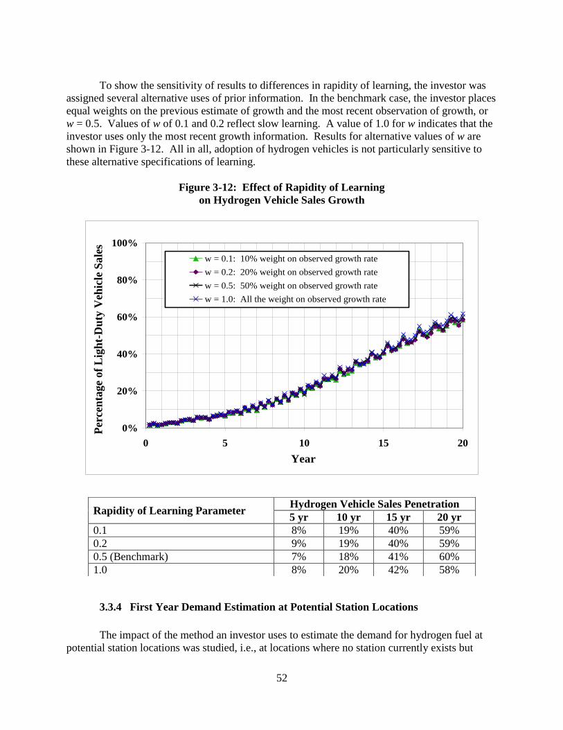
52
To show the sensitivity of results to differences in rapidity of learning, the investor was
assigned several alternative uses of prior information. In the benchmark case, the investor places
equal weights on the previous estimate of growth and the most recent observation of growth, or
w = 0.5. Values of w of 0.1 and 0.2 reflect slow learning. A value of 1.0 for w indicates that the
investor uses only the most recent growth information. Results for alternative values of w are
shown in Figure 3-12. All in all, adoption of hydrogen vehicles is not particularly sensitive to
these alternative specifications of learning.
Figure 3-12: Effect of Rapidity of Learning
on Hydrogen Vehicle Sales Growth
0%
20%
40%
60%
80%
100%
0 5 10 15 20
Year
Per
cen
tag
e o
f L
igh
t-D
uty
Veh
icle
Sa
les
w = 0.1: 10% weight on observed growth rate
w = 0.2: 20% weight on observed growth rate
w = 0.5: 50% weight on observed growth rate
w = 1.0: All the weight on observed growth rate
3.3.4 First Year Demand Estimation at Potential Station Locations
The impact of the method an investor uses to estimate the demand for hydrogen fuel at
potential station locations was studied, i.e., at locations where no station currently exists but
Rapidity of Learning Parameter Hydrogen Vehicle Sales Penetration
5 yr 10 yr 15 yr 20 yr
0.1 8% 19% 40% 59%
0.2 9% 19% 40% 59%
0.5 (Benchmark) 7% 18% 41% 60%
1.0 8% 20% 42% 58%

53
where a station could be sited. In the model, the investor has the ability to observe the traffic
going by locations to estimate future hydrogen demands. Two alternative methods of observing
traffic were simulated, an ―HPV Only‖ strategy and an ―All Traffic‖ strategy. In the ―HPV
Only‖ strategy, the investor counts only the number of hydrogen vehicles going past a given
location. In the ―All Traffic‖ strategy, the investor counts all drivers going past a particular
location. See Section B.2.1.1, ―Unadjusted Sales at a Location,‖ of Appendix B for additional
information.
While there are slight differences, Figure 3-13 shows that the method of estimating first
year demand at potential station locations using traffic counts has relatively little impact on the
growth of hydrogen vehicle sales.
Figure 3-13: Effect of Method of Estimating First Year Demand at Potential New Station
Locations on Hydrogen Vehicle Sales Growth
0%
20%
40%
60%
80%
100%
0 5 10 15 20
Year
Per
cen
tag
e o
f L
igh
t-D
uty
Veh
icle
Sa
les
Demand Estimate: HPV Only
Demand Estimate: All Traffic (Benchmark)
First Year Demand Estimation
Method at Potential New Station
Locations
Hydrogen Vehicle Sales Penetration
5 yr 10 yr 15 yr 20 yr
All Traffic (Benchmark) 7% 18% 41% 60%
HPV Only 6% 14% 43% 63%

54
3.3.5 Expectation of Growth
Another calculation characterizing the sophistication of the investor’s planning pertains
to how the investor forms the expectation of hydrogen sales growth. To study sensitivity, two
approaches have been used. In the first approach, the investor makes a projection each year of
sales in the upcoming year based on the most recent year’s growth and assumes that the new
level of sales will prevail in all future years. Expected sales are ratcheted up each year based on
expected one year growth, but no allowance is made for the fact that the whole future growth
path will be affected. The investor thus does not allow for the fact that growth will continue in
the future. In the second approach, the investor uses a logistic growth method. The same
hydrogen sales expectation for the next year is used as in the first approach, but a logistic growth
function is used to forecast subsequent hydrogen sales. This process is also repeated each year.
The logistic model of growth expectation is used in the benchmark case. The results presented in
Figure 3-14 show that the method chosen does not have much effect on adoption. Sections
B.2.1.4, ―Estimating Future Sales Using a Logistic Growth Function,‖ and B.2.1.5, ―Estimating
Future Sales Using a Simpler Approach,‖ of Appendix B describe these procedures.
Figure 3-14: Effect of How Growth Expectations Are Modeled on
Hydrogen Vehicle Sales Growth
0%
20%
40%
60%
80%
100%
0 5 10 15 20
Year
Per
cen
tag
e o
f L
igh
t-D
uty
Veh
icle
Sa
les
Expectation of Growth: Logistic (Benchmark)
Expectation of Growth: Linear
Expectation of Growth Hydrogen Vehicle Sales Penetration
5 yr 10 yr 15 yr 20 yr
Logistic (Benchmark) 7% 18% 41% 60%
Linear 7% 16% 39% 58%

55
3.3.6 Number of Investors
To evaluate the influence of the number of investors on hydrogen vehicle adoption,
scenarios with 2 and 10 investors were run in addition to the single investor scenario of the
benchmark case. As shown in Figure 3-15, the number of investors in a simulation has relatively
little effect on hydrogen vehicle sales penetration. A key to understanding this result is that each
investor, even a single investor, prices hydrogen at average cost, responding to potential
competition from other investors and to the threat of regulation if higher prices are charged,
implying that additional investors do not add price competition to an already competitive market,
as discussed earlier in Section 2.3.2, ―Price Charged for Hydrogen Fuel.‖
This result does not however mean that investors act independently of one another. They
are still competing with each other for sales available at any location. With multiple investors,
an individual investor first evaluates the profitability of potential new station locations as if no
other investors were present. Next, for locations that pass the profitability tests, the investor
locates a station with probability equal to one over the number of investors, assuming other
investors will also be building station. Using a random number generator, this procedure yields
on average one new station located at each profitable location, although depending on
randomness occasionally no station or more than one station might be sited there. See Section
B.3, ―Number of Investors,‖ of Appendix B.
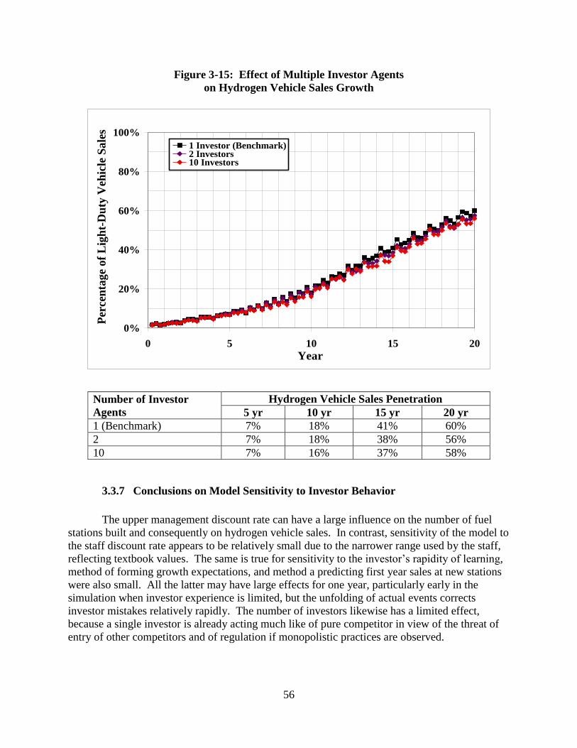
56
Figure 3-15: Effect of Multiple Investor Agents
on Hydrogen Vehicle Sales Growth
0%
20%
40%
60%
80%
100%
0 5 10 15 20
Year
Per
cen
tag
e o
f L
igh
t-D
uty
Veh
icle
Sa
les
1 Investor (Benchmark)2 Investors10 Investors
3.3.7 Conclusions on Model Sensitivity to Investor Behavior
The upper management discount rate can have a large influence on the number of fuel
stations built and consequently on hydrogen vehicle sales. In contrast, sensitivity of the model to
the staff discount rate appears to be relatively small due to the narrower range used by the staff,
reflecting textbook values. The same is true for sensitivity to the investor’s rapidity of learning,
method of forming growth expectations, and method a predicting first year sales at new stations
were also small. All the latter may have large effects for one year, particularly early in the
simulation when investor experience is limited, but the unfolding of actual events corrects
investor mistakes relatively rapidly. The number of investors likewise has a limited effect,
because a single investor is already acting much like of pure competitor in view of the threat of
entry of other competitors and of regulation if monopolistic practices are observed.
Number of Investor
Agents
Hydrogen Vehicle Sales Penetration
5 yr 10 yr 15 yr 20 yr
1 (Benchmark) 7% 18% 41% 60%
2 7% 18% 38% 56%
10 7% 16% 37% 58%

57
3.4 Use of Realistic Approximative Decisions
What is the effect of realistic, approximative decision making, sometimes called
satisficing, in place of traditional, full optimization on the results? Obtaining an answer to this
question faces the difficulty that derivation of the time path of full optimization is far too
complicated to be able to estimate. While it is not possible to obtain an exact answer, a
sensitivity analysis was performed to simulate an upper bound on the penetration that would
result from an investor siting hydrogen fueling stations using perfect information. Having
perfect information would imply that an investor could completely resolve two chief
uncertainties, the growth rate of demand for hydrogen, and identification of fueling locations
with the greatest potential for spurring hydrogen vehicle adoption. This upper bound is
simulated by a hydrogen vehicle adoption path achieved in the case of an Unlimited Supply at
Each Location, as it is not feasible for an investor to push the rate of adoption any higher than by
providing hydrogen fueling opportunities comparable in availability to that of gasoline. The
actual adoption path generated by an investor with perfect information would be below this
adoption path, but it is impossible to construct the perfect-information adoption path. This
maximum possible path gives an upper bound that can be compared with actual adoption paths
generated with various types of approximative behavior.
The results of the effect of the investor’s approximative behavior are shown in Figure 3-
16, which shows penetration achieved for the stock of hydrogen vehicles at a given year (as
opposed to sales penetration used for the other sensitivity comparisons). In the benchmark case,
each investor agent follows a rule-of-thumb algorithm, and a stock penetration of 25% is reached
by the 20th
year. In the unlimited fueling availability case, the upper bound of stock penetration
by the 20th
year is 33%. At the 20th
year, the actual stock penetration of 25% would be reached
no earlier than the 18th
year, indicating that the delay at the 20th
year due to satisficing behavior
is at most 2 years.
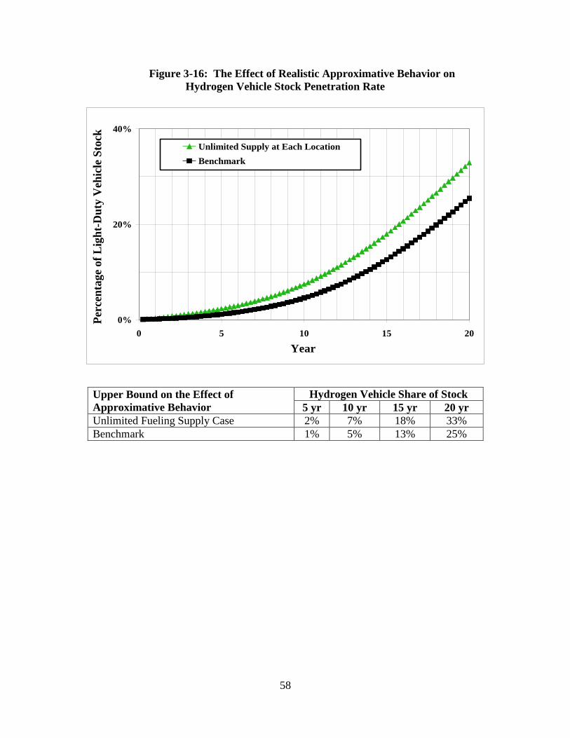
58
Figure 3-16: The Effect of Realistic Approximative Behavior on
Hydrogen Vehicle Stock Penetration Rate
0%
20%
40%
0 5 10 15 20
Year
Per
cen
tag
e o
f L
igh
t-D
uty
Veh
icle
Sto
ck
Unlimited Supply at Each Location
Benchmark
Upper Bound on the Effect of
Approximative Behavior
Hydrogen Vehicle Share of Stock
5 yr 10 yr 15 yr 20 yr
Unlimited Fueling Supply Case 2% 7% 18% 33%
Benchmark 1% 5% 13% 25%

59
PART FOUR: SENSITIVITY TO MARKET AND POLICY
INFLUENCES
This Part of the report presents model results intended to show the main uses of the study.
These are estimating the effects of market developments that could importantly affect the
adoption of hydrogen vehicles, and policy initiatives that could influence adoption.
The market developments considered here pertain to two chief ways that markets can
affect profitability of adoption, namely, through purchase prices of vehicles and through prices
of the fuels used by the vehicles. Section 4.1 is concerned with the difference between the price
of a new hydrogen vehicle and a new non-hydrogen vehicle, called sticker price difference. A
constant difference and a declining difference over time are considered. Section 4.2 is concerned
with differences in operating costs between hydrogen and non-hydrogen vehicles.
The policies considered are of 3 kinds. Section 4.3 presents estimates of the effects of tax
credits for the purchase of hydrogen vehicles. Section 4.4 presents estimates of effects of carbon
taxes. Section 4.5 presents estimates of the effects of the number of initial hydrogen seed
stations, which might be financed wholly or partly by government entities.
4.1 Market Developments: Sticker Price Difference
4.1.1 Constant Sticker Price Difference
In the benchmark scenario, it is assumed that at some point hydrogen vehicles will be
competitive with non-hydrogen vehicles, although the model makes no prediction of the date that
competitiveness will be reached. For the two vehicles to be on exactly equal terms, the sum of
the sticker price difference and the present value of operating costs would be zero. It is
reasonable, however, to assume that some advantage to hydrogen vehicles would be needed in
order for there to be a gain to drivers from switching away from the type of vehicle they are
already driving. In the benchmark case in this study, the hydrogen and non-hydrogen vehicle
have the same purchase price, with hydrogen fuel cost savings giving the hydrogen vehicle an
edge.
As shown in Figure 4-1, a sticker price difference of $2,000 in favor of the hydrogen
vehicle, sales penetration reaches 92% by the 20th
year compared to the benchmark penetration
rate of 60% with equal vehicle sticker prices. A sticker price difference of $6,500 in favor of a
non-hydrogen vehicle results in only 6% hydrogen vehicle sales penetration by the 20th
year.

60
Figure 4-1: Effect of Sticker Price on Hydrogen Vehicle Sales Growth
0%
20%
40%
60%
80%
100%
0 5 10 15 20
Year
Per
cen
tag
e o
f L
igh
t-D
uty
Veh
icle
Sa
les $2,000 Lower
No Difference (Benchmark)
$6,500 Higher
Sticker Price of
Hydrogen Vehicle
Hydrogen Vehicle Sales Penetration
5 yr 10 yr 15 yr 20 yr
$2,000 Lower 26% 61% 82% 92%
No Difference
(Benchmark) 7% 18% 41% 60%
$6,500 Higher 1% 3% 4% 6%
4.1.2 Declining Sticker Price Difference
For hydrogen vehicles to sell at the same price as non-hydrogen vehicles, fuel cell costs
will need to fall substantially. Given that hydrogen vehicles require about 80 to 100 kW of
power, a PEM fuel cell cost of $1,000/kW, gives a fuel cell cost of $100,000 per vehicle.16
Costs
of other components raise the total cost of a hydrogen vehicle further, giving a cost several times
that needed to be viable in a mass market. At present, such products do not exist much beyond
the prototype stage. A 2009 DOE report has emphasized that the cost of a hydrogen fuel cell is
expected to decline significantly in the future.2 Three factors have been recognized as
contributing to future declines: 1) economies of scale that progressively lower production costs
as production volume increases; 2) learning by doing in manufacturing which lowers costs as
more experience with a new product is gained, and 3) technological advancements that increase
16 National Academy of Engineering, The Hydrogen Economy: Opportunities, Costs, Barriers, and R&D Needs (Washington,
D.C.: National Research Council, 2004), pp. 4, 98, 119.

61
durability and reliability and reduce the cost of major components. These major components
including polymer electrolyte membranes, catalyst electrodes, the fuel cell stack, the fuel cell
processor, the power conditioner, and air supply systems. Appendix C reviews estimates of the
potential for contributions of these factors.
Based on Appendix C, scenarios of decline in the sticker price difference between
hydrogen and non-hydrogen vehicles were chosen in which, after an unspecified number of
years, the difference in sticker price becomes low enough to attract a significant number of
buyers of hydrogen vehicles. In the scenarios, further declines occur as the three factors
mentioned in the preceding paragraph continue to operate.
Results of the declining sticker price scenarios are presented in Figure 4-2 below. In the
benchmark case, sales penetration reaches 60% by the 20th year of the simulation. In the 5 year
case, the sticker price difference declines at a constant rate from a $14,000 to $0 over the first
five years of the simulation. After five years, the hydrogen vehicle and the non-hydrogen
vehicle have the same sticker price for the remainder of the simulation. In the 10 year case, the
same sticker price difference declines at a constant rate over ten years instead of five years. In
the 20 year case, there is a decline in sticker price difference from $14,000 to $4,000 over a 20
year period. As shown in the figure, there is a moderate response for the 5 year and 10 year
declining sticker price difference scenarios, reaching 58% and 52% sales penetration,
respectively. For the 20 year case, the effect is strong resulting in only 10% sales penetration by
the 20th year of the simulation.

62
Figure 4-2: Effect of Declining Sticker Price Difference on Hydrogen Vehicle Sales Growth
0%
20%
40%
60%
80%
100%
0 5 10 15 20
Year
Per
cen
tag
e o
f L
igh
t-D
uty
Veh
icle
Sa
les None (Benchmark)
5 Years
10 Years
20 Years
Years to Reach Same Price
as Non-Hydrogen Vehicle
Hydrogen Vehicle Sales Penetration
5 yr 10 yr 15 yr 20 yr
None (Benchmark) 7% 18% 41% 60%
5 Years 5% 17% 37% 58%
10 Years 2% 11% 31% 52%
20 Yearsa 0% 1% 3% 10%
a Decline to $4,000 disadvantage
4.2 Market Developments: Fuel Prices
In the benchmark scenario, driver agents can save 9.8 cents per mile on fuel by driving a
hydrogen vehicle instead of a non-hydrogen vehicle. In calculating this amount, the benchmark
gasoline price is based on the EIA Annual Energy Outlook 2010 reference case.17
The savings
17 Energy Information Administration, http://www.eia.doe.gov/oiaf/aeo/aeoref_tab.html, Table 3, Energy Prices by Sector and
Source. Gasoline price for an assumed initial showroom year of 2018 is $3.91 per gallon, giving a mid-year price in the
adoption process for use in the simulation of $4.85 in 2025, using EIA’s projected 2.7% annual gasoline price increase (2009
prices).
63
per mile are calculated using a hydrogen price equal to H2A hydrogen production cost18
and fuel
efficiency estimates for non-hydrogen and hydrogen vehicles.19
The present value of the fuel savings comes to $3,383 over the life of the vehicle for the
average driver, who drives 12,150 miles a year. In the benchmark case, the sticker prices of the
hydrogen and non-hydrogen vehicle are equal. The fuel savings make the hydrogen vehicle a
good enough financial investment to lead to 60% penetration by the 20th
year. Any combination
of sticker prices and fuel savings that leads to a $3,383 gain from switching to hydrogen will lead
to the same results as in the base case.
Results for two scenarios in addition to the benchmark case are presented: one in which
fuel prices are such that drivers save a high 20.7 cents per mile by driving a hydrogen vehicle,
and one in which they save a low 0.5 cents per mile. The gain per mile made possible in the high
savings case translates into a present value of approximately $7,174 for the average driver agent.
The low savings per mile translates into a present value of only $183.
18 $3.63 per kg (2009 prices). U.S. Department of Energy, ―Future (2025) Natural Gas Steam Reformer (SMR) at Forecourt
1,500 kg/day,‖ Department of Energy Hydrogen Program, May 27, 2008.
http://www.hydrogen.energy.gov/h2a_prod_studies.html (accessed February 17, 2009). 19 29 mpg and 52 miles per kg, Norman Brinkman, Michael Wang, Trudy Weber, and Thomas Darlington, ―Wells-to-Wheels
Analysis of Advanced Fuel/Vehicle Systems – A North American Study of Energy Use, Greenhouse Gas Emissions, and
Criteria Pollutant Emissions,‖ Argonne National Laboratory, 2005, p. 89, Table 3-3.

64
Figure 4-3: Effect of Fuel Cost Savings on Hydrogen Vehicle Sales Growth
0%
20%
40%
60%
80%
100%
0 5 10 15 20
Year
Per
cen
tag
e o
f L
igh
t-D
uty
Veh
icle
Sa
les 20.7 cents per mile fuel savings
9.8 cents per mile fuel savings
0.5 cents per mile fuel savings
Per Mile Fuel Savings Hydrogen Vehicle Sales Penetration
5yr 10yr 15yr 20yr
20.7 cents per mile 25% 55% 76% 86%
9.8 cents per mile
(Benchmark) 7% 18% 41% 60%
0.5 cents per mile 2% 3% 6% 10%
Results for the fuel cost cases are shown in Figure 4-3. As compared to the 60%
penetration by the 20th
years in the base case, 86% penetration is reached by the 20th
year in the
high-savings scenario and only 10% in the low-savings scenario.
4.3 Policies: Tax Credits for Hydrogen Vehicle Purchase
To turn now from effects of market developments to effects of policies, a tax credit
toward a vehicle purchase works in the same way as a drop in sticker price, since drivers who
buy the vehicle can subtract the tax credit from their income tax and get a dollar for dollar
savings. A precedent can be found in tax credits that have been offered for the purchase of
hybrid electric vehicles.

65
4.3.1 Permanent Tax Credit
The benchmark scenario in Figure 4-4 is again shown as the lower line. Also shown is
the result for a scenario in which a $2,500 tax credit is offered for purchasing a hydrogen
vehicle. The effectiveness of the tax credit is reflected in the result that by the 20th
year, 88% of
all light-duty vehicles sold are powered by hydrogen, as compared with 60% in the benchmark
case. Results for a higher tax credit of $6,000 are also shown, in which the hydrogen sales share
reaches 99% in the 20th
year.
Figure 4-4: Effect of Permanent Tax Credits on Hydrogen Vehicle Sales Penetration
0%
20%
40%
60%
80%
100%
0 5 10 15 20
Year
Per
cen
tag
e o
f L
igh
t-D
uty
Veh
icle
Sa
les
Tax Credit for Purchase of Hydrogen Vehicles = $6,000
Tax Credit for Purchase of Hydrogen Vehicles = $2,500
Tax Credit for Purchase of Hydrogen Vehicles = $0 (Benchmark)
Permanent Tax Credit Hydrogen Vehicle Sales Penetration
5 yr 10 yr 15 yr 20 yr
$6,000 Tax Credit 63% 91% 97% 99%
$2,500 Tax Credit 21% 54% 77% 88%
$0 Tax Credit (Benchmark) 7% 18% 41% 60%
4.3.2 Temporary Tax Credit
Figure 4-5 below shows the consequence of eliminating a vehicle tax credit after 10
years. While the drop in the percent of sales once the tax credit is terminated may appear to be
large, hydrogen sales penetration continues to climb after termination of the credit, reaching 69%
of sales after 20 years with the $2,500 credit and 79% with the $6,000 credit. The temporary tax

66
credit hastens the growth of the hydrogen vehicle stock, which in turn hastens driver agents’
familiarity with the vehicle through the bandwagon effect and contributes to accelerated growth
throughout the simulation. Relative effects on the stock of hydrogen vehicles are even more
noticeable. Without a tax credit, the hydrogen vehicle stock would make up about 5% of the total
vehicle stock after 10 years, as was shown in Figure 3-2. The tax credits raise the stock at 10
years to 13% and 29%, respectively, which in turn raise the level of the hydrogen sales
penetration above the no-credit benchmark case in the remaining years.
Figure 4-5: Effect of Temporary Tax Credits on Hydrogen Vehicle Sales Penetration
0%
20%
40%
60%
80%
100%
0 5 10 15 20Year
Per
cen
tag
e o
f L
igh
t-D
uty
Veh
icle
Sa
les
Ten Year Tax Credit for Purchase of Hydrogen Vehicles = $6,000Ten Year Tax Credit for Purchase of Hydrogen Vehicles = $2,500No Tax Credit (Benchmark)
Temporary Tax Credit
Terminated after 10 years
Hydrogen Vehicle Sales Penetration
5 yr 10 yr 15 yr 20 yr
$6,000 Tax Credit 63% 91% 66% 79%
$2,500 Tax Credit 21% 54% 53% 69%
$0 Tax Credit (Benchmark) 7% 18% 41% 60%

67
4.4 Policies: Carbon Taxes
Two carbon tax levels have been investigated: $38 and $116 per metric ton of CO2,
calculated with the Greenhouse Gases, Regulated Emissions, and Energy Use in Transportation
(GREET) Model.20 These compare with $85 per metric ton estimated by the Stern Report as the
social (i.e., total) cost of carbon, and $110 per metric ton estimated as the requirement to have an
impact on large-scale power generation from renewables.21
The smaller tax of $38 per metric
ton corresponds to a tax of 33 cents per gallon of gasoline and 44 cents per kg of hydrogen
produced at distributed SMR stations. The larger tax of $116 per metric ton corresponds to a tax
of $1.01 per gallon of gasoline and $1.34 per kg of hydrogen produced at distributed stations.
With the H2A model’s assumption of 90% effective carbon capture and sequestration at
centralized production facilities, the $38 and $116 taxes translate into 6 cent and 18 cents per kg
taxes, respectively, on centrally produced hydrogen.
As noted in Part Two, centrally produced hydrogen is more expensive at the pump than is
distributed production, and hence will not be profitable without a tax that has a greater effect on
distributed costs. As shown in Figure 4-6 below, the lower carbon tax of $38 per metric ton is
not large enough to noticeably affect sales penetration compared to the benchmark case of no
tax. The larger tax of $116 per metric ton, which makes centrally produced hydrogen profitable
in the very first year, results in modestly higher levels of hydrogen vehicle sales penetration.
20 Argonne National Laboratory, ―The Greenhouse Gases, Regulated Emissions, and Energy Use in Transportation (GREET)
Model,‖ ―http://www.transportation.anl.gov/modeling_simulation/GREET/ index.html, December 2009. 21 David J. C. MacKay, Sustainable Energy: Without the Hot Air (Cambridge: UIT Cambridge Press, 2009), p. 224, Figure 29.2.

68
Figure 4-6: Effect of Carbon Taxes on Hydrogen Vehicle Sales Penetration
0%
20%
40%
60%
80%
100%
0 5 10 15 20
Year
Per
cen
tag
e o
f L
igh
t-D
uty
Veh
icle
Sa
les
$116 Tax per Metric Ton CO2No Tax (Benchmark)$38 Tax per Metric Ton CO2
Carbon Tax Hydrogen Vehicle Sales Penetration
5 yr 10 yr 15 yr 20 yr
$116 Tax per Metric Ton CO2 9% 24% 46% 64%
No Tax (Benchmark) 7% 18% 41% 60%
$38 Tax per Metric Ton CO2 8% 19% 39% 59%
4.5 Policies: Seed Stations
Seed stations, established through policy assistance, assure drivers within range of those
stations of a supply of hydrogen fuel and may tip their vehicle purchase decisions in favor of a
hydrogen vehicle in early periods before hydrogen becomes more widely available. The
benchmark case includes 15 seed stations, which correspond to current locations of hydrogen
stations in the Los Angeles area. The existing stations are smaller than the standard 1,500 kg/day
stations used for later periods and are not all accessible to the public. Nevertheless, in the
absence of better data, these stations are included in the initial conditions of the model for two
reasons. First, they represent a guess as to where new commercially viable stations may be sited
through public-private partnerships. Second, although smaller than the subsequently located
private stations, the effect of these seed stations on early adoption of hydrogen vehicles is likely
to be about the same as larger stations later since there will only be a few potential adopters of
hydrogen vehicles early on and station capacity would not materially affect drivers’ utility
calculations. In any event, as described below, the location of the seed stations does not seem to
make a large difference to the adoption path.

69
Sensitivity of the model to the introduction of 15 additional stations (totaling 30 seed
stations) is tested. In one case, these additional 15 stations are placed in what the model deems
to be the most profitable 15 locations for stations in early years (i.e., the first 15 locations where
the investor would want to locate a station). In the other case, these 15 stations are placed where
the model deems it least profitable (i.e., the last 15 locations at which the investor sites a station).
The results are shown in Figure 4-7 below. For comparison, a scenario is also included in which
refueling is ubiquitous, i.e., no matter where a driver would like to refuel, more than enough
stations are available.
Both of these scenarios result in sales penetration rates that are very close to the
benchmark after 20 years, and the locations of seed stations have a smaller effect on adoption
than the number of seed stations. The case where the additional seed stations are placed in the
least profitable locations (the last 15 locations to get stations otherwise), the 20-year sales
penetration is 63%, slightly higher than the case in which the seed stations are placed in more
profitable locations (the first 15 locations to get stations otherwise), 59%, and the benchmark of
60%. This small effect may be due to driver agents being highly mobile and able to substitute
one location for another easily, or more simply, due to the outcome that regular stations sprout
soon enough to make it immaterial whether, at any location, a seed station existed or not at the
beginning of the simulation. The magnitude of the effect of seed station locations also may be
influenced by the strength of the inconvenience effect.
Siting additional seed stations at the least profitable locations does spur marginally higher
adoption, as placing stations where the market would otherwise hesitate to place them leads to
some drivers buying hydrogen vehicles in cases where otherwise they may not have due to being
underserved. The siting of initial seed stations has a more pronounced effect on the stock of
hydrogen vehicles because the additional stations spur adoption in early years.
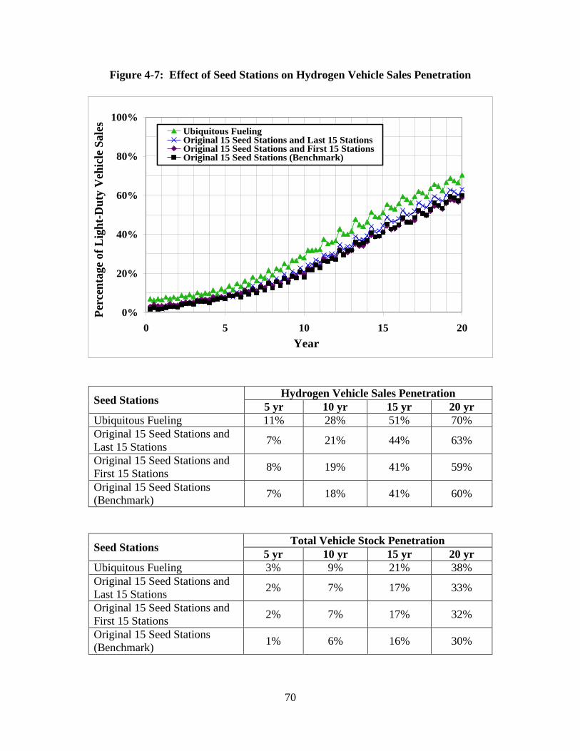
70
Figure 4-7: Effect of Seed Stations on Hydrogen Vehicle Sales Penetration
0%
20%
40%
60%
80%
100%
0 5 10 15 20
Year
Per
cen
tag
e o
f L
igh
t-D
uty
Veh
icle
Sa
les
Ubiquitous FuelingOriginal 15 Seed Stations and Last 15 StationsOriginal 15 Seed Stations and First 15 StationsOriginal 15 Seed Stations (Benchmark)
Seed Stations Hydrogen Vehicle Sales Penetration
5 yr 10 yr 15 yr 20 yr
Ubiquitous Fueling 11% 28% 51% 70%
Original 15 Seed Stations and
Last 15 Stations 7% 21% 44% 63%
Original 15 Seed Stations and
First 15 Stations 8% 19% 41% 59%
Original 15 Seed Stations
(Benchmark) 7% 18% 41% 60%
Seed Stations Total Vehicle Stock Penetration
5 yr 10 yr 15 yr 20 yr
Ubiquitous Fueling 3% 9% 21% 38%
Original 15 Seed Stations and
Last 15 Stations 2% 7% 17% 33%
Original 15 Seed Stations and
First 15 Stations 2% 7% 17% 32%
Original 15 Seed Stations
(Benchmark) 1% 6% 16% 30%

71
4.6 Conclusions
Equal prices of hydrogen and non-hydrogen vehicles, as in the benchmark case, allows a
60% sales penetration by the 20th
year because of fuel savings with hydrogen vehicles. Among
alternative sticker price difference scenarios, beginning with a $14,000 hydrogen vehicle price
disadvantage that declines to 0 disadvantage by either 5 or 10 years still allows sales penetration
to reach over 50% by the 20th
year. A non-declining price disadvantage of $6,500 precludes a
hydrogen take-off.
Permanent tax credits of $2,500 and $6,000 dramatically hasten sales penetration. Tax
credits that end after 10 years lead to a drop in new sales penetration when the credits expire, but
the 20th
-year sales penetration is still higher than in the benchmark case with no tax credits. This
is because so many more hydrogen vehicles are purchased earlier and, operating through the
bandwagon and familiarity effects, continue to affect vehicle choice after the expiration of the
tax credits.
Fuel cost savings, as influenced by the prices hydrogen and non-hydrogen fuels such as
gasoline, play an important role in the adoption of hydrogen vehicles. Sufficiently low savings
will prevent take-off, while very high savings have an effect similar to the smaller tax credit.
Carbon taxes have limited effects. A low carbon tax of $38 per metric ton of CO2
translates into taxes of 44 cents per kg of hydrogen and 33 cents per gallon of gasoline. It favors
hydrogen relative to gasoline because of hydrogen’s fuel efficiency advantage, which makes the
rise in costs of a hydrogen vehicle less than the rise in cost of a gasoline-powered vehicle. The
tax falls more on distributed than centralized hydrogen production because carbon emissions per
kg from distributed production are assumed to be less than for centralized production. A high
carbon tax of $116 per metric ton of CO2 results in taxes of $1.34 per kg of hydrogen at
distributed stations and $1.01 per gallon of gasoline. Centralized production, bearing lesser tax,
becomes profitable in the first year of simulation. The hydrogen it produces is taxed at only
$0.18 per kg, giving hydrogen a greater advantage over gasoline. Consequently, the higher
carbon tax generates somewhat higher 20th
-year hydrogen sales penetration than the base case.
An additional 15 stations available at the beginning of the simulation has a perceptible,
though not major effect in increasing the 20th
-year stock of hydrogen vehicles. Alternative
locations of the seed stations have little impact on 20th
-year sales penetration.

72
PART FIVE: VALIDATION
A model that projects how events could unfold far in the future under alternative
conditions must find its validation in parallels between its results and other similar phenomena
that have occurred in the past. This chapter reports the results of an investigation of the validity
of the hydrogen model by comparing its results with experiences of other innovations.
Section 5.1 tests the benchmark adoption path of the hydrogen model against adoption
paths of consumer durables reported in the literature. Section 5.2 compares the projections of the
hydrogen model with the experiences of three other automotive innovations: compressed natural
gas (CNG) vehicles, Japanese vehicles adopted in the United States, and other hybrid vehicles.
Section 5.3 summarizes the results of the validation exercises.
5.1 Relation of Adoption Paths of this Study to Previously Estimated
Adoption Paths
Much of the previous literature on adoption of new products involves use of data on the
total number of adopters in each time period. One of the most enduring diffusion models to
come out of this literature is the Bass Model, which uses three parameters—an innovation factor,
an imitation factor, and a potential market size—to create an adoption path with a logistic
pattern.22
The Bass Model allows for both innovators and imitators in the population of
innovation adopters. The timing of an innovator’s adoption decision is not influenced by the
number of people who have already bought the product. Imitators are, however, influenced by
the number of previous adopters, learning in a sense from those who have already bought. These
features of the Bass Model are in the driver module in the form of the bandwagon effect (Section
2.2.2.4, ―Bandwagon Effect‖), and the taste for greenness among some drivers (Section 2.2.2.5,
―Greenness‖), whereby the early hydrogen vehicle purchases of innovators with a high taste for
greenness provide examples and information for subsequent adopters through the bandwagon
effect. Extensively in the existing literature, Bass Model parameters have been estimated
through statistical regression analysis for many consumer durables, using data on total purchases
in a time period.
The present study on the other hand has used a completely different approach, based on
the thousands of individual driver agents in the model. The validation exercise builds an
adoption path for hydrogen vehicles from the ground up, modeling the choices of several
thousand individuals rather than using market-wide totals. The test is whether this approach
reproduces patterns found in other studies. It does, in fact, generate a logistic-shaped adoption
path.
22 Frank M. Bass, ―A New Product Growth Model for Consumer Durables,‖ Management Science 15 (1969): 215-227.
Reprinted in Management Science 50, No. 12 Supplement (2004): 1825-1832.

73
5.1.1 The Logistic Function and the Comparison of Adoption Paths
Because it takes time for consumers to adopt innovative new products, much literature
has been devoted to studying the adoption rates of these products. The adoption of a new
technology or innovation, when plotted in a cumulative graph, has been observed to follow a
logistic, or S-shaped pattern.23
This phenomenon is observed repeatedly because word of mouth,
or personal observation, must spread about any worthwhile innovation before everyone who
might find it useful actually adopts it. The adoption rate begins slowly at first, when there are
only a few initial adopters who are either willing to take chances on the new product or simply
quick to inform themselves about it. Then, as initial adopters share their knowledge with non-
adopters, the rate of adoption grows substantially until the adopters outnumber the non-adopters.
At that point adoption begins to slow because fewer non-adopters remain to switch behaviors and
adopt. This pattern has been observed with a variety of new innovations, from hybrid seed
corn24
to the telegraph and the telephone. The S-shaped adoption path is an observation that
occurs with successful innovations in which the news spread by the initial adopters is good news.
Unsuccessful innovations will instead see a shift downward which will lead to discontinuance of
the product.
During the development of the hydrogen model the observation of S-shaped adoption
paths was used as a validation method. It was found that the agents, both drivers and investors,
in responding to their individual criteria, yielded a market adoption path that had the elongated
S-shape. That the model produces this pattern is the most basic level of validation, since it
provides the indication that the complex system of interactions between agents that has been
built produces intuitive results that match real world behavior in at least one major respect.
It is, of course, important to note that there is more than one set of agent behaviors that
would produce an S-shaped adoption path, and not all of those sets may be realistic or sensible.
During the course of model development, sensitivity tests were carried out in which some model
structures that produce S-shaped adoption paths broke down under various conditions. This
produced more specific insights into the proper model structure, as reported for many of the
parameter and policy variable variations in Parts Three and Four.
While model results have a logistic growth path in common with past product adoptions,
adoption paths can still vary greatly. A wide variety of adoption rates are observed for previous
innovations, and little information is available on which to base judgments about what speed of
adoption to expect for hydrogen vehicles. Even if the technology is successful, thought needs to
be given to the similarities and differences between hydrogen technology and the types of
technologies that have seen rapid or slow adoption. Care should be exercised when comparing
adoption data for a diverse set of products. For example, consider targeting an adoption rate of
―60% of households‖ as an indicator of successful adoption. This metric could be misleading in
some cases, since the potential market for some technologies may not include all households. If,
for example, during the first decade of a product’s introduction it is only affordable for, say, half
23 Everett M. Rogers, Diffusion of Innovations (New York: Free Press, 2003), Chapter 7, ―Innovativeness and Adopter
Categories: The S-Shaped Curve of Adoption and Normality,‖ pp. 272-275. 24 Zvi Griliches, ―Hybrid Corn: An Exploration in the Economics of Technological Change,‖ Econometrica 25 (1957): 501-522.

74
of all households, and most of that group has adopted by the end of the decade, then adoption
might be considered largely complete, with the later widening of the product’s affordability
being considered a separate phenomenon. This and other matters of interpretation make the
analysis and comparison of adoption paths highly subjective. In order to eliminate as much
subjectivity as possible, this report makes extensive use of the product diffusion modeling
literature.
5.1.2 Comparison of Hydrogen Vehicles with Consumer Durables as a Whole
Over the years the Bass Model has been used to analyze many consumer durables and
industrial products with a wide variety of adoption paths. A meta-analysis of 213 innovations
has synthesized Bass Model applications into a set of adoption paths for various categories of
products.25
That analysis reports an adoption curve for consumer durables as a whole that is
defined by a Bass curve with an innovation parameter of 0.03 and an imitation parameter of 0.38,
controlling for characteristics of the original study, the type of innovation, and where the
innovation occurred—Europe or the United States. Consequently, the parameter magnitudes of
0.03 and 0.38 represent underlying structural tendencies of innovations. However, these
estimates remain composites across many applications of the Bass Model, and certain product
characteristics—such as whether sales data were from Great Britain or the United States and
whether the innovation analyzed was an industrial product or consumer durable—were found to
affect the magnitudes of the innovation and imitation parameters. The adoption path for
consumer durables as a whole in the United States was found to be a Bass curve with an
innovation parameter of 0.007 and an imitation parameter of 0.295. Figure 5-1 shows this
adoption curve.
25 Fareena Sultan, John U. Farley and Donald R. Lehmann, ―A Meta Analysis of Diffusion Models,‖ Journal of Marketing
Research 27 (1990): 70-77.
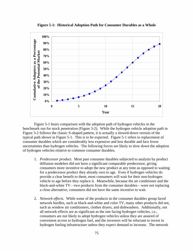
75
Figure 5-1: Historical Adoption Path for Consumer Durables as a Whole
0%
10%
20%
30%
40%
50%
60%
70%
80%
90%
100%
0 5 10 15 20
Year
Cu
mu
lati
ve A
do
pte
rs
as
a P
ercen
tag
e
of
the P
ote
nti
al
Ma
rk
et
Figure 5-1 bears comparison with the adoption path of hydrogen vehicles in the
benchmark run for stock penetration (Figure 3-2). While the hydrogen vehicle adoption path in
Figure 3-2 follows the classic S-shaped pattern, it is actually a slowed-down version of the
typical path shown in Figure 5-1. This is to be expected. Figure 5-1 refers to replacement of
consumer durables which are considerably less expensive and less durable and face fewer
uncertainties than hydrogen vehicles. The following forces are likely to slow down the adoption
of hydrogen vehicles relative to common consumer durables.
1. Predecessor product. Most past consumer durables subjected to analysis by product
diffusion modelers did not have a significant comparable predecessor, giving
consumers more incentive to adopt the new product at any time as opposed to waiting
for a predecessor product they already own to age. Even if hydrogen vehicles do
provide a clear benefit to them, most consumers will wait for their non-hydrogen
vehicle to age before they replace it. Meanwhile, because the air conditioner and the
black-and-white TV—two products from the consumer durables—were not replacing
a close alternative, consumers did not have the same incentive to wait.
2. Network effects. While some of the products in the consumer durables group faced
network hurdles, such as black-and-white and color TV, many other products did not,
such as window air conditioners, clothes dryers, and dishwashers. Additionally, not
all network effects are as significant as the one facing hydrogen vehicles, i.e.,
consumers are not likely to adopt hydrogen vehicles unless they are assured of
convenient access to hydrogen fuel, and the investors will be reluctant to invest in
hydrogen fueling infrastructure unless they expect demand to increase. The network

76
effect for color TV, for example, involved the appearance of broadcasting in color, an
event that was less gradual than the appearance of fuel stations, and color
broadcasting, which could be received by black-and-white sets, grew for many years
before any significant number of people began to adopt, meaning that by the time
adoption took off the hurdle was largely already cleared.
3. Drastic improvement over past products. Hydrogen vehicles will perform largely the
same functions as non-hydrogen vehicles do today, whereas many past innovations in
consumer durables performed completely new functions that were of an unknown but
certainly large value to consumers. This lack of novel application is likely to dampen
the enthusiasm of drivers to adopt hydrogen relative to many previous new products.
5.2 Adoption Experience under Other Vehicle Information
5.2.1 Compressed Natural Gas Vehicles
5.2.1.1 Review of Experience
Interest in compressed natural gas (CNG) vehicles arose in the early 1980s from the steep
rise in oil prices following the Iranian Revolution and the beginning of the Iran-Iraq War in 1979
and 1980. The public benefits of energy security enhancements from reduced oil imports and
environmental benefits from reduced automotive emissions combined with private incentives
from lower natural gas prices relative to oil to offer promise for the introduction of this
alternative fuel vehicle. Additionally, the regulation of natural gas prices appeared to offer
greater price stability than with oil.
During this period, and as early as the 1970s in some countries, natural gas vehicles saw
increased adoption worldwide, especially prominently in Argentina and New Zealand where
combinations of recent natural gas strikes, government support (tax allowances for consumers
and suppliers but not direct fuel subsidies) and foreign exchange problems provided a
combination of opportunities and incentives. However, changing economic incentives during the
1990s greatly reduced the competitiveness of CNG vehicles in both Argentina and New
Zealand.26
Although the CNG vehicle was introduced around the same time in the United States, it
did not receive widespread acceptance for a combination of reasons. First, as shown in Figure 5-
2, the large price differential of oil over natural gas in the United States that existed at the
beginning of the 1980s had eroded by mid-decade. Deregulation of natural gas that began with
the 1978 Natural Gas Policy Act took place in stages from the 1980s to 1993 removing the
possibly illusory promise of price stability from natural gas. So the CNG vehicle attempted to
enter the U.S. market with no advantage in either fuel price or fuel price stability.
26 J.C. Fraccia, ―An Overview of the Argentine NGV Experience,‖ (paper presented at World Bank Workshop on CNG Vehicles,
2000); Garth Harris, ―Compressed Natural Gas in New Zealand,‖ (paper presented at World Bank Workshop on CNG
Vehicles, 2000).
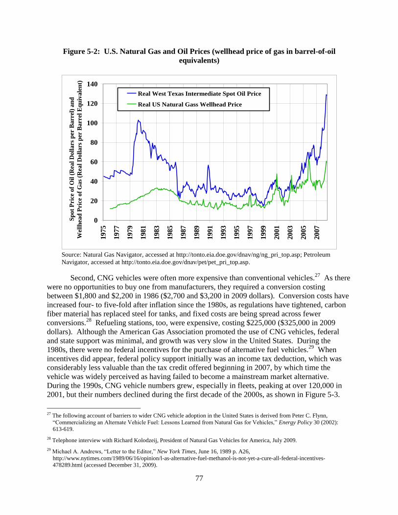
77
Figure 5-2: U.S. Natural Gas and Oil Prices (wellhead price of gas in barrel-of-oil
equivalents)
0
20
40
60
80
100
120
140
1975
1977
1979
1981
1983
1985
1987
1989
1991
1993
1995
1997
1999
2001
2003
2005
2007
Sp
ot
Pri
ce o
f O
il (
Rea
l D
oll
ars
per
Ba
rrel
) an
d
Wel
lhea
d P
rice
of
Ga
s (R
eal
Doll
ars
per
Ba
rrel
Eq
uiv
ale
nt)
Real West Texas Intermediate Spot Oil Price
Real US Natural Gass Wellhead Price
Source: Natural Gas Navigator, accessed at http://tonto.eia.doe.gov/dnav/ng/ng_pri_top.asp; Petroleum
Navigator, accessed at http://tonto.eia.doe.gov/dnav/pet/pet_pri_top.asp.
Second, CNG vehicles were often more expensive than conventional vehicles.27
As there
were no opportunities to buy one from manufacturers, they required a conversion costing
between $1,800 and $2,200 in 1986 ($2,700 and $3,200 in 2009 dollars). Conversion costs have
increased four- to five-fold after inflation since the 1980s, as regulations have tightened, carbon
fiber material has replaced steel for tanks, and fixed costs are being spread across fewer
conversions.28
Refueling stations, too, were expensive, costing $225,000 ($325,000 in 2009
dollars). Although the American Gas Association promoted the use of CNG vehicles, federal
and state support was minimal, and growth was very slow in the United States. During the
1980s, there were no federal incentives for the purchase of alternative fuel vehicles.29
When
incentives did appear, federal policy support initially was an income tax deduction, which was
considerably less valuable than the tax credit offered beginning in 2007, by which time the
vehicle was widely perceived as having failed to become a mainstream market alternative.
During the 1990s, CNG vehicle numbers grew, especially in fleets, peaking at over 120,000 in
2001, but their numbers declined during the first decade of the 2000s, as shown in Figure 5-3.
27 The following account of barriers to wider CNG vehicle adoption in the United States is derived from Peter C. Flynn,
―Commercializing an Alternate Vehicle Fuel: Lessons Learned from Natural Gas for Vehicles,‖ Energy Policy 30 (2002):
613-619. 28 Telephone interview with Richard Kolodzeij, President of Natural Gas Vehicles for America, July 2009. 29 Michael A. Andrews, ―Letter to the Editor,‖ New York Times, June 16, 1989 p. A26,
http://www.nytimes.com/1989/06/16/opinion/l-as-alternative-fuel-methanol-is-not-yet-a-cure-all-federal-incentives-
478289.html (accessed December 31, 2009).

78
The sharp increase in the number of CNG vehicles beginning in the early 1990s is most likely
the result of the Energy Policy Act of 1992, which required the federal government to begin
buying alternative fuel vehicles for its fleets in 1993.30
There are currently over 100,000 CNG
vehicles in the United States, but this stock has never reached six one-hundredths of a percent of
the national vehicle stock.
Figure 5-3: U.S. CNG Vehicles on the Road
0
20
40
60
80
100
120
140
1988 1993 1998 2003
Veh
icle
s (T
hou
san
ds)
0.00%
0.01%
0.02%
0.03%
0.04%
0.05%
0.06%
Per
cen
t of
Tota
l V
ehic
le S
tock
Compressed Natural Gas Percent of all Vehicles on the Road
Sources: See Footnote
31
Third, natural gas fuel stations were not quickly profitable. It was believed that it would
take up to five years for an individual station to reach capacity utilization of 100,000 liters-
equivalent per month. Few stations were on target in reaching utilization and profitability goals,
and policy attention to the issue of balance between investor profitability and consumer interests
was late in coming. Lack of retained earnings meant that marketing resources were low, and
eventually the interest of fuel retailers waned. The refueling infrastructure proved at least as
important as the vehicle technology.
30 Brian Anthony Abbanat, ―Alternative Fuel Vehicles: The Case of Compressed Natural Gas (CNG) Vehicles in California
Households,‖ M.S. Thesis, University of California Davis, 2001, p. 10. 31 For 1989, Thomas C. Hayes. ―Natural Gas Sales Set at Denver AMOCO Sites,‖ New York Times, December 21, 1989, p, D7.
http://www.nytimes.com/1989/12/21/business/natural-gas-sales-set-at-denver-amoco-sites.html (accessed December 31,
2009.); for 1992-2003, Energy Information Administration. ―Estimated Number of Alternative Vehicle Fuels in Use and Fuel
Consumption, 1992-2007.‖ June 2009. http://www.eia.doe.gov/emeu/aer/txt/ptb1005.html (accessed March 10, 2010); Total
vehicles on the road: Transportation Energy Data Book 28. (Oak Ridge, Tenn.: Oak Ridge National Laboratory) last updated
June 29, 2009. http://cta.ornl.gov/data/Index.shtml (accessed December 31, 2009).

79
Fourth, CNG was adopted initially more by commercial fleets than individuals. In
California in particular this was for two reasons: taxation of private dispensing often was
ignored by state authorities, and the capital cost of a public refueling network was widely seen as
prohibitive, especially inasmuch as a large proportion of the fleet to be refueled would not use
publicly available fueling stations.
5.2.1.2 Comparison of CNG Vehicle Experience with the Hydrogen Model
of this Study
In sum, between external market events, the technology itself, and policy support, neither
the vehicles nor the supporting fueling infrastructure were particularly profitable as private
investments. The proximate market impetus for the CNG vehicle in the United States was a
temporary, sharp increase of the oil price over the U.S. natural gas price while the market forces
behind hydrogen are the possibility of long-term, permanent increases in the oil price and
increasing concerns with carbon emissions. CNG technology in the 1980s and 1990s was more
of a fuel substitution in an internal combustion engine than the radical technological change of
the hydrogen vehicle. Policy support for adoption of CNG vehicles was scattered and not
particularly strong during the early years of its adoption. Finally, the low adoption of non-fleet
CNG vehicles lengthened the pay-back period on infrastructure investments in fueling facilities.
In contrast to CNG vehicles, hydrogen vehicles have had considerable policy support
through R&D, and the modeling here explores further temporary policy support during early
market transition. The price of the principal competing transportation fuel, oil, is not expected to
decline, and the full cost of operating the hydrogen vehicle—sticker price plus fuel cost—is
advantageous relative to that of the competing non-hydrogen vehicle. The modeling of hydrogen
fuel stations shows them to be profitable early over a broad range of conditions, and they become
sufficiently widely distributed in early simulation periods to allay a good deal of driver anxiety.
Altogether, initial similarities between CNG vehicles and what should be expected from
hydrogen vehicles dwindle upon examination.
5.2.2 The Market Penetration of Japanese Vehicles in the United States
5.2.2.1 Review of Experience
Before 1968, Japanese imports to the United States accounted for less than 1% of U.S.
retail auto sales. Japanese imports, and domestically produced Japanese models beginning in the
mid-1980s, experienced their period of major expansion in the U.S. auto market from 1968 to
1991. Over a span of one year, 1967 to 1968, sales of Japanese imports more than doubled, from
0.8% to 1.8% of new car sales. By 1982, Japanese imports peaked at 22.6% of the U.S.
market.32
32 Ward’s Automotive Yearbooks (Southfield, Mich.: Ward’s Communications, 1968-2008).

80
Figure 5-4: Growth of the Market Share of Japanese Light-Duty Vehicles in the United
States, 1965-2008
0%
10%
20%
30%
40%
50%
60%
1960 1970 1980 1990 2000 2010
Per
cen
tag
e o
f J
ap
an
ese
Lig
ht-
Du
ty V
ehic
le S
ale
s in
the
Un
ited
Sta
tes
Japanese new car sales Japanese imports
Source: Ward’s Automotive Yearbooks, 1968-2008.
With Japanese auto presence skyrocketing, the United States instituted an automobile
import quota on Japan in 1981. The Reagan-backed Voluntary Export Restraint (VER) limited
Japanese auto imports to 1.68 million a year which, as Figure 5-4 above shows, curtailed the
pace of market penetration of Japanese vehicles for several years in the mid-1980s. The cap was
periodically raised and reached 2.3 million before it was terminated in 1992.33
The VER turned out to be a gift to Japanese auto makers. During the late 1970s and early
1980s, Toyota and Honda produced high quality vehicles and began to cultivate strong U.S.
demand. The VER raised prices and lowered sales volumes of Toyotas and Honda in the United
States, but did not hurt profits.34
In response to increasing U.S. demand for Japanese vehicles and the constraints of the
VER, Japanese automakers began to produce in the United States. Honda began manufacturing
vehicles in the United States in 1982,35
and has produced 14 million in the country since then.36
33 Steven Berry, James Levinsohn, and Ariel Pakes, ―Voluntary Export Restraints on Automobiles: Evaluating a Trade Policy,‖
American Economic Review 89 (1999): 400-430. 34 Berry et. al., Ibid. 35 Ward’s Automotive Yearbook, 1982. 36 Ward’s Automotive Yearbook, 1982-2008.

81
Toyota began manufacturing in the United States in 1984,37
and has produced 15 million
domestically.38
Nissan, which began manufacturing in the United States in 1983,39
has produced
more than 5 million vehicles.40
Mitsubishi, Subaru and Isuzu also have U.S. production plants.41
As Figure 5-4 demonstrates, adding the U.S.-produced vehicles to the Japanese imports reveals
an overall picture of Japanese growth into the U.S. auto market.
Factoring in this U.S. production, Japanese autos account for almost one-half of new-
vehicle sales in the U.S. market. The full Japanese market share, including imports and
domestically produced autos, peaked in the United States in 1991 at 39.6% of U.S. light-duty
vehicle sales. During the 1990s the Japanese market share dipped, dropping to 34% of new sales
in 1997, probably because of a lengthy period of lower oil prices. In the past decade Japanese
sales have climbed again, reaching almost 45% of new auto sales.
5.2.2.2 Comparison of Japanese Import Experience with the Hydrogen
Model of this Study
Japanese vehicle adoption in the United States shows the classic S-shape, where adoption
starts slowly, eventually takes off, and then plateaus. This path is common for new product
penetration. The speed of market penetration of new Japanese vehicles was less rapid than the
benchmark case in the current hydrogen model: a little under 30% of new sales in the twenty
years between 1965 (using that as a rough start date) and 1985, compared with 60% in the
hydrogen model’s benchmark simulation. It is possible, however, that the VER period may have
set back that market penetration by about 5 years, judging from the shape of the curve in Figure
5-4.
The comparison here is between two innovations in the automobile market, although the
case of the hydrogen vehicle is a more drastic change in technology than was the introduction of
Japanese models. While the Japanese vehicles were 30% to 75% more fuel-efficient than the
U.S. Big Three fleet average, the smaller Japanese vehicles may not have offered comparable
features demanded by many American consumers, sheer physical size being prominent among
them. The growth of sales penetration by Japanese vehicles in the 1975-85 decade was
somewhat slower than the sales penetration projected for hydrogen vehicles during their first
decade, possibly because of the imperfect substitutability of the Japanese for the American-made
vehicles (the hydrogen and non-hydrogen vehicles are specified as essentially perfect substitutes
in features other than fuel efficiency). In the 1985-95 decade, the slower growth of Japanese
37 Ward’s Automotive Yearbook, 1984. 38 Ward’s Automotive Yearbooks, 1984-2008. 39 Ward’s Automotive Yearbook, 1983. 40 Ward’s Automotive Yearbooks, 1983-2008. 41 Ward’s Automotive Yearbook, 2008.

82
sales share compared to the hydrogen model can be accounted for additionally by the converging
fuel efficiency of the American vehicles.42
5.2.3 Hybrid Vehicles
5.2.3.1 Review of Experience
In 2008, 312,000 hybrid vehicles were sold in the United States, 1.94% of all light-duty
vehicles sold, down slightly from 352,000 in 2007, as shown in Figure 5-5. Slightly over half of
these were Toyota Priuses. The Honda Insight was introduced in 1999, and the Prius in 2000.43
Figure 5-5: United States Hybrid Vehicle Sales Volume
0
50
100
150
200
250
300
350
400
1999 2000 2001 2002 2003 2004 2005 2006 2007 2008
Vo
lum
e in
Th
ou
san
ds
Other
Honda Insight
Saturn Aura
Lexus LS600hL
Saturn Vue
Nissan Altima
Toyota Camry
Lexus GS 450h
Mercury Mariner
Toyota Highlander
Lexus RX 400h
Honda Accord
Ford Escape
Honda Civic
Toyota Prius
Source: U.S. Department of Energy, Alternative Fuels & Advanced Vehicles Data Center, HEV Sales by
Model accessed July 28, 2009 at http://www.afdc.energy.gov/afdc/data/vehicles.html.
Worldwide, hybrid vehicle sales have taken off sharply since the Prius was introduced in
Japan in 1997, with most of the sales coming in North America, as shown in Figure 5-6. The
global downturn in the second half of 2008 led to a decline in North American sales, but Prius
sales continue to grow worldwide. The annual growth rates have been high, quadrupling
42 U.S. EPA Office of Transportation and Air Quality, ―Light-Duty Automotive Technology and Fuel Economy Trends, 1975
through 2008,‖ U.S. EPA, EPA420-S-08-003, September 2008, http://www.epa.gov/otaq/fetrends.htm (accessed August 5,
2009). 43 U.S. Department of Energy Office of Energy Efficiency and Renewable Energy, ―Alternative Fuels & Advanced Vehicles
Data Center, HEV Sales by Model,‖ U.S. Department of Energy. http://www.afdc.energy.gov/afdc/data/vehicles.html
(accessed July 28, 2009).

83
between 2003 and 2005. This corresponded to a change in the production method—starting with
the 2004 model, Toyota began producing the Prius on a standard mass production assembly line,
resulting in one being produced every minute instead of one every 8 to 10 minutes as before.44
The use of a standard assembly line has dropped the manufacturing cost significantly, allowing
Toyota to deliver a substantially upgraded model, which in turn has generated publicity and
popularity. Another major limiting factor in hybrid production is third-party component
availability, particularly batteries. Currently, all production of Priuses is in Japan, although plans
are in progress to open factories in other countries.45
Figure 5-6: Annual Worldwide Prius Sales
0
50
100
150
200
250
300
350
400
450
1997 1998 1999 2000 2001 2002 2003 2004 2005 2006 2007 2008 2009
Vo
lum
e in
Th
ou
san
ds
Japan North America Europe Other
Source: Ward’s Automotive Yearbooks, 1997-2008.
The U.S. light duty vehicle market includes at least 20 hybrid vehicles, including sedans,
luxury cars, SUVs, and trucks. While sedans are the most popular, Figure 5-7 shows that SUVs
such as the Toyota Highlander, the Ford Escape, and the Lexus RX400h are popular as well.
44 Wired News Report, ―Toyota Says Hybrids Can Be Cheap,‖ Wired, October, 2, 2003.
http://www.wired.com/cars/energy/news/2003/10/60667 (accessed July 28, 2009). 45 Mike Millikin, ―US Sales of Hybrids Down 8.9% in September,‖ Green Car Congress News, October 3, 2008.
http://www.greencarcongress.com/2008/10/us-sales-of-hyb.html (accessed July 28, 2009).

84
Figure 5-7: Composition of Hybrid Car Sales Volume in the United States in 2008
Toyota Prius
51%
Toyota Camry
15%
Honda Civic
10%
Toyota Highlander
6%
Ford Escape
5%
Other
5%
Lexus RX400h
5%
Nissan Altima
3%
Source: Ward’s Automotive Yearbook, 2008.
Hybrid vehicles generally have a higher manufacturer’s suggested retail price (MSRP)
than comparable conventionally powered vehicles, but make up for that with better fuel mileage.
Table 5-1 below shows the mileage and MSRP for various popular hybrid vehicles.
Table 5-1: Selection of Hybrid Vehicles, Prices, and Mileages
Vehicle MPG (city/hwy) MSRP
Honda Accord Hybrida 29/37 $31,540
Honda Civic Hybrida 50/50 $22,400
Toyota Priusa 60/51 $22,305
Toyota Camry Hybridb 40/38 $25,653
Toyota Highlander Limited 4X2a 33/28 $33,595
Toyota Highlander Limited 4X4a 31/27 $34,995
Lexus RX 400h FWDb 32/27 $40,586
Lexus RX 400h AWDb 31/27 $41,942
Lexus GS 450hb 25/28 $53,877
Ford Escape FWDa 36/31 $27,515
Ford Escape 4WDa 33/29 $29,140
Mercury Mariner AWDa 33/29 $29,840
aWard’s Automotive Yearbook, 2006. bWard’s Automotive Yearbook, 2007.
All prices in 2005 dollars.

85
A federal tax credit is available to purchasers of hybrid vehicles, varying in magnitude
with the size of the vehicle and the cumulative production volume, as shown in Table 5-2.46
Table 5-2: Federal Tax Credits as of June 2006
Vehicle Fed. Tax Credit (as
of March 2006)
Toyota Prius $3,150
Toyota Camry Hybrid $2,600
Toyota Highlander Hybrid $2,600
Ford Escape Hybrid47 $2600/$1950
Lexus RX 400h $2,200
Honda Civic Hybrid $2,100
Mercury Mariner Hybrid $1,950
Lexus GS 450h $1,550
Honda Insight $1,450
Honda Accord Hybrid48 $1350/$650
Source: U.S. Internal Revenue Service, ―2006 Model Year Hybrid Vehicles,‖
http://www.irs.gov/newsroom/article/0,,id=176418,00.html (accessed June 2007).
Table 5-3 combines the price and tax credit data above and compares the difference in
price to the savings from lowered fuel cost available to hybrid drivers. The price and fuel
efficiency of each hybrid vehicle in this table are compared to those of the conventional vehicle
closest to the hybrid model.
46 Consumers seeking the federal tax credit may need to buy early since the full credit is only available for a limited time.
Taxpayers may claim the full amount of the allowable credit up to the end of the first calendar quarter after the quarter in
which the manufacturer records its sale of the 60,000th hybrid or advanced lean-burn technology. For the second and third
calendar quarters after the quarter in which the 60,000th vehicle is sold, taxpayers may claim 50% of the credit. For the fourth
and fifth calendar quarters, taxpayers may claim 25% of the credit. No credit is allowed after the fifth quarter. 47 $2,600 for the 4WD and $1,950 for the FWD; see U.S. Internal Revenue Service (IRS), (2007), ―2006 Model Year Hybrid
Vehicles,‖ http://www.irs.gov/newsroom/article/0,,id=176418,00.html (accessed June, 2007). 48 The Accord gets $650 when not calibrated and $1,350 when it is calibrated; see IRS, ibid.

86
Table 5-3: Hybrid Vehicle Cost Savings
Selection of Hybrid
Vehicles
Vehicle Price
Differencea
Difference in
Gallons of Gasoline
per 12,000 Miles a
Savings per Mile a
Accord Hybrid $3,690 107.0 $0.043
Civic Hybrid $3,590 107.8 $0.043
Prius / Corolla XRS $3,985 183.8 $0.074
Camry Hybrid $2,318 128.7 $0.052
Highlander Limited $2,570 157.6 $0.063
RX 400h AWD $3,662 144.3 $0.058
GS 450h $1,852 105.3 $0.04.2
Escape 4WD $4,240 112.9 $0.046
Mariner AWD $6,095 158.4 $0.064
Average $3,556 134.0 $0.054 a Ward’s Automotive Yearbook, 2006, 2007.
Although hybrid SUVs get substantially lower fuel mileage than hybrid sedans (around
30 mpg), this represents a relatively large savings when considered in terms of how many gallons
of gasoline are used by the average driver driving 12,000 miles per year.
5.2.3.2 Comparison of Hybrid Vehicle Experience with the Hydrogen Model
of this Study
Sensitivity analysis to fuel efficiency and sticker price differences allows comparison of
the model results for hydrogen vehicle adoption with the market experience of hybrid vehicle
adoption. In Los Angeles, the hybrid sales penetration in 2009, which is a tenth-year market
penetration, reached an estimated 4.9%.49
The 2009 Los Angeles sales penetration is roughly two-thirds the magnitude of the tenth-
year sales penetration of hydrogen vehicles in the benchmark simulation of the model. The
perfect substitutability between the hydrogen and non-hydrogen vehicles assumed in the model
makes the adoption of the hydrogen vehicle more sensitive to fuel efficiency differences than
hybrids may be, and as noted, the hybrids’ sticker prices are relatively higher. Conducting a
hydrogen simulation with a $3,500 price disadvantage for hydrogen vehicles, the same as the
price differential of hybrids in Table 5-3, and the 5.4 cents per mile fuel efficiency advantage,
yields a tenth-year penetration of 4.1%.
The 4.9% result for observed hybrid sales and the simulated 4.1% result for hydrogen
vehicle sales are of the same general order of magnitude, under the conditions that the price
disadvantage and fuel efficiency advantage for a hydrogen vehicle are the same as for a hybrid
49 Bradley Berman, ―December 2009 Dashboard: Year-End Tally,‖ HybridCars.com Market Dashboard, January 20, 2010,
http://www.hybridcars.com/hybrid-sales-dashboard/december-2009-dashboard.html (accessed March 2, 2010). Los Angeles
market share estimated assuming approximately 750,000 new vehicle sales used in the model, reduced by 21% to account for
the reduction in national sales in 2009.

87
vehicle. A hybrid vehicle bears a greater similarity to a gasoline-powered vehicle than a
hydrogen vehicle does to a non-hydrogen vehicle. Drivers are more familiar with technology
and performance characteristics of hybrid vehicles than they would be with hydrogen vehicles
early in the adoption process with hydrogen vehicles. Furthermore, hydrogen vehicles require
special fueling stations that are less frequently encountered than conventional fuel stations
capable of serving hybrid vehicles. Accordingly a somewhat lower penetration by the tenth year
could be expected for hydrogen vehicles.
5.3 Conclusions on Validation
As discussed in Part Five, research was conducted on adoption of other durable goods
innovations to see if the adoption path predicted for hydrogen vehicles in this study is similar to
those for other innovations. A comparative study was conducted on the adoption paths of
consumer durables products as a whole. Adoption experiences and lessons learned were
gathered for specific vehicle innovations including CNG vehicles, penetration of Japanese
vehicles in the U.S. market, and hybrid vehicles.
Overall, we judge the validation tests to be favorable to the Agent-based model of this
study. The adoption paths for hydrogen vehicles in the simulations of this study have been found
to have a typical S-shaped adoption curve similar to the empirical adoption paths calculated for
other consumer durables. The S-curve for hydrogen vehicles exhibits a slower rate of adoption
than for the average of all consumer durables. This is to be expected because automobiles
including hydrogen vehicles have a much longer life and are thus subject to slower turnover than
other durable goods. A lesson from the three vehicle case studies (CNG vehicles, Japanese
vehicles, and hybrids) is that gain to the consumer from an innovation and, in the case of
Japanese imports, government policy can have a powerful influence on the rate of adoption.
88
PART SIX: SUMMARY AND CONCLUSIONS
The present Part of the study first brings together and summarizes the findings from Part
Two describing the agent-based model, Parts Three and Four on numerical results, and Part Five
on validation. This Part then turns to the implications of the findings for the central concern of
the study:
Whether the private sector will supply the infrastructure to permit
a transition to hydrogen consistent with national goals and, if not,
what policy actions would be effective.
Finally, future work is discussed, with emphasis on the use of the study as an aid in
analyzing policies under changing conditions in the future.
6.1 The Agent-based Model
As described in Part Two, the agent-based model (ABM) developed for this study
simulates the behavior of more than 7 million Los Angeles drivers using over 7 thousand
individual driver agents. The driver and investor modules and their interactions highlight the
strengths of the ABM approach in allowing for realistic approximative decisions that depart from
perfect optimization. The actors have imperfect knowledge. They can learn from their mistakes.
The model projects events forward in time period by period building on outcomes from previous
periods. The model permits projections of ultimate market penetration of hydrogen vehicles and
the length of time required to achieve the penetration.
In deciding whether to buy a hydrogen vehicle, vehicle driver agents consider the sticker
price difference between hydrogen and non-hydrogen vehicles, the difference in fuel costs,
beliefs about how well a hydrogen vehicle operates, their preference for greenness, and the
availability of hydrogen fuel as determined by the number and location of stations where
hydrogen fuel is sold. Investor agents who supply hydrogen infrastructure compare actual sales
of hydrogen fuel each period with what they expected and decide on the number and location of
stations to build in the next period. If sales are favorable, more hydrogen fuel stations are
supplied each period, further reinforcing demand growth as driver agents purchase more
hydrogen vehicles. The predictions of number of hydrogen vehicles replicate the S-shaped
pattern of adoption generally observed for innovations.
6.2 Benchmark Case
The benchmark case, chosen as a base from which to examine sensitivity, was described in
Section 3.1. The benchmark uses driver and investor behavior parameters, combined with prices
of vehicles and fuels for hydrogen and non-hydrogen vehicles that would result in cost
competitiveness and allow a hydrogen vehicle take-off. This study does not attempt to predict
the year when the required cost competitiveness permitting take-off will be achieved. That will
89
depend on progress in reducing costs of producing hydrogen vehicles, on future prices of
competitor vehicles, and on future hydrogen and non-hydrogen fuel prices, among other things.
These are subject to unpredictable change over the course of the many years involved in the
transformation to hydrogen transportation. The present study is designed to ascertain the
conditions under which the hydrogen fuel infrastructure necessary for the transition will be
supplied once the pre-conditions for a transition are achieved. The results can be used to show
how the transformation will be affected as conditions change in the future and also to explore
policy alternatives.
In the benchmark case, hydrogen vehicle sales penetration as a percent of all new vehicle
sales rises first at an accelerating rate up until approximately year 20, when sales penetration
reaches 60%, after which penetration continues to rise but at a declining rate. It reaches 86% by
year 40 after which it is rather flat.
Much of the present study has been devoted to examining the sensitivity of the benchmark
case to the numerical parameters used. Of the 130 parameters of the model, selected parameters
have been identified as being of particular importance. In view of the difficulty of predicting
conditions 40 years in the future and the greater policy relevance of nearer term events,
penetration for the first 20 years of transition has been used for the sensitivity comparisons.
6.3 Sensitivity to Driver Behavior
Sensitivity to driver parameters was considered in Section 3.2. Of the 17 parameters
describing driver behavior, three have been identified as being of special importance: (1) driver
familiarity with hydrogen vehicles; (2) the bandwagon effect indicating how greatly undecided
drivers are influenced by the favorable experience of drivers who have already bought hydrogen
vehicles; and (3) taste for greenness, meaning how much the driver’s decision is swayed by the
vehicle’s environmental friendliness.
6.3.1 Familiarity with Hydrogen Vehicle Performance
Driver lack of familiarity with the performance characteristics of hydrogen vehicles has
an effect on early sales that has a compound effect on later adoption. Whereas in the benchmark
scenario, hydrogen vehicles account for 60% of sales within the 20-year period being used for
comparison, the range of 20-year penetration between low and high familiarity is 24% to 79%.
6.3.2 Bandwagon Effect
By the 20th
year, the range of sales penetration between low and high bandwagon strength
is found to be greater than for familiarity, namely 27% to 94%. Most of the impact is between
the 10th and 15th years of the transition.

90
6.3.3 Greenness
Differences in the level and distribution of the taste for greenness affect the number of
drivers adopting in the early years, giving a change that is compounded by the bandwagon effect
and can have large lasting consequences for sales penetration. The sensitivity is less than that of
familiarity or bandwagon effects. For the 20-year comparison period, the greenness penetration
range is 17% to 69%.
6.4 Sensitivity to Investor Behavior
Sensitivity to investor parameters was considered in Section 3.4. A major finding is that
the rapidity of adoption can be greatly affected by upper management’s degree of risk aversion
and optimism or pessimism about the hydrogen vehicle. These attitudes are reflected in the
discount rate used by upper management. High discount rates equivalent to risk-averse short pay-
back periods could keep sales penetration to the range of only 2% to 11% after 20 years,
effectively preventing a hydrogen take-off. On the other hand, one or more other companies
with more optimistic upper management could come in and start the adoption process.
Many investor practices have more limited impact on the pace of adoption of hydrogen
vehicles. There is less sensitivity to the narrower range of discount rates used by the line staff in
its evaluations submitted to upper management, because the staff uses less extreme textbook
discount rates. Relatively limited effects are also found for the rapidity of the investor’s learning
(weight on new observations), sophistication of expectations formation (whether future growth
will be logistic), and method of estimating first year demand at locations where there is not yet a
station (observing either total vehicles or only hydrogen vehicles). All the latter effects may be
large for one year, particularly early in the simulation when investor experience is limited, but
the unfolding of actual events corrects investor mistakes relatively rapidly. Because a single
investor is already acting much like a pure competitor in view of the threat of entry of other
investors and of regulation if monopolistic practices are observed, whether there is a single
investor or a number of investors has limited impact.
6.5 Effect of Realistic Approximative Decisions in the Agent-based Model
Section 3.4 was concerned with whether the use of realistic approximative decision rules,
sometimes called satisficing, in place of full optimization, interferes with the ultimate penetration
of hydrogen vehicles. Obtaining a strict answer to this question is not feasible, because the
calculation of the time path of adoption under perfect information would requires solution of an
impossibly complex set of conditions. In order to address the, a test was carried out to obtain an
upper bound on the possible effect. Having perfect issue information would imply that an
investor could perfectly estimate the growth rate of demand for hydrogen and the fueling
locations with the greatest potential for spurring hydrogen vehicle adoption. An upper bound is
simulated by a hydrogen vehicle adoption path achieved by running a case with unlimited
hydrogen supply at each location. This maximum possible path gives an upper bound that can
be compared with actual adoption paths generated with approximative behavior.

91
In the benchmark case, where the investor agent uses approximative rules of thumb, a
stock penetration of 25% is reached by year 20. In the unlimited fueling availability case, 25%
stock penetration is achieved approximately 2 years earlier. This is the maximum effect of the
investor’s lack of perfect information during the first 20 years.
6.6 Use of the Model to Examine Market Developments
Sensitivities to two types of market developments were investigated: 1) prices of
hydrogen and non-hydrogen vehicles and 2) operating costs as affected by prices of the fuels
used by the vehicles.
6.6.1 Vehicle Prices
Scenarios of the effects of sticker price differences between the two types of vehicles
demonstrate the vital importance of vehicle prices to the adoption process. These were
investigated in Section 4.1. In the benchmark case, the sticker prices of hydrogen and non-
hydrogen vehicles are equal. The major incentive to adopt a hydrogen vehicle is its greater fuel
efficiency. The market share attained by hydrogen vehicles by the 20th
year is then 60%. In a
scenario where the hydrogen vehicle has a sticker price that is $2,000 less than the non-hydrogen
vehicle, the market share attained by the 20th
year is a high 92%. On the other hand, in a
scenario where the hydrogen vehicle is $6,500 more than the non-hydrogen vehicle, market share
in the 20th
year is reduced to only 6%.
The foregoing vehicle price scenarios assume that the sticker prices remain constant
throughout the simulation. Realism can be added by taking account of the fact that the price of a
newly innovated product typically continues to fall for some time. To add this realism,
additional scenarios of decline in the sticker price difference were investigated in which the cost
of hydrogen vehicles declines first to the point where an initial subset of drivers adopts,
providing a beginning to the innovation process. The cost of hydrogen vehicles then continues to
drop as further adoption proceeds.
The first declining sticker price scenario is that the sticker price differences will decline
at a constant percentage rate from a $14,000 hydrogen vehicle disadvantage to no sticker price
difference, in 5 years. This contrasts with the benchmark case in which the situation of no price
difference has already been reached by the start of the simulation and there are no further
declines. The second declining sticker price scenario is that the decline is from a $14,000
disadvantage to no price difference over 10 years. In both of these scenarios, penetration
exceeds 50% by year 20 and is thus not too different from the benchmark case.
In the final declining price scenario, the decline is from a $14,000 sticker price difference
to $4,000 over 20 years. In this scenario, penetration by year 20 is only 10%. The indication is
that attention to the rate of price decline during the innovation process can be important to the
rapidity of adoption.

92
6.6.2 Prices of Gasoline and Hydrogen Fuel
With the prices of gasoline and hydrogen fuel used in the benchmark case, driver agents
can save 9.8 cents per mile on fuel by driving a hydrogen vehicle instead of a non-hydrogen
vehicle. In Section 4.2, results for two fuel price scenarios in addition to the benchmark case
were presented: one in which drivers save 20.7 cents per mile by driving a hydrogen vehicle, and
the other in which they save 0.5 cents per mile. As compared to the 60% penetration by the 20th
years in the base case, 86% penetration is reached by the 20th
year in the high-savings scenario,
and only 10% in the low-savings scenario. The results are driven by the price of gasoline and
suggest that future gasoline prices could be a crucial market consideration determining hydrogen
vehicle penetration.
6.7 Policies
Three types of policies have been considered that would affect the rapidity of hydrogen
vehicle adoption: 1) tax credits, 2) carbon taxes and 3) government assistance with initial seed
stations.
6.7.1 Tax Credits
Tax credits for the purchase of a hydrogen vehicle were considered in Section 4.3. The
effectiveness of a $2,500 tax credit is reflected in the result that by the 20th
year, 88% of all light-
duty vehicles sold are powered by hydrogen, as compared with 60% in the benchmark case. For
a higher tax credit of $6,000, the hydrogen vehicle sales share is 99% in the 20th
year.
Under a more modest approach, the tax credit would be available only for the first 10
years. Hydrogen sales penetration would then reach 69% of sales after 20 years with the $2,500
credit and 79% with the $6,000 credit.
6.7.2 Carbon Taxes
Two carbon tax levels have been investigated: $38 and $116 per metric ton of CO2.
Results were presented in Section 4.4. The tax of $38 per metric ton on carbon translates into a
tax of 33 cents per gallon on gasoline, 44 cents per kg on hydrogen produced at distributed SMR
stations, and 6 cents per kg on hydrogen produced at centralized facilities. The tax of $116 per
metric ton translates into a tax of $1.01 per gallon of gasoline, $1.34 per kg of hydrogen at
distributed stations, and 18 cents per kg on centrally produced hydrogen.
The lower carbon tax of $38 per metric ton is not large enough to noticeably affect sales
penetration compared to the benchmark case of no tax. The larger tax of $116 per metric ton
makes centrally produced hydrogen profitable in the very first year and results in modestly
higher levels of hydrogen vehicle sales penetration.

93
6.7.3 Seed Stations
Seed stations, established through policy assistance, assure drivers within range of those
stations of a supply of hydrogen fuel and may tip their vehicle purchase decisions in favor of a
hydrogen vehicle in early periods before hydrogen more widely available. The benchmark case
includes 15 seed stations, which correspond to current locations of hydrogen stations in the Los
Angeles area.
In Section 4.5, sensitivity to the introduction of 15 additional stations, totaling 30 seed
stations, was examined. The additional 15 stations were placed alternatively in the most
profitable and least profitable locations. Both scenarios gave sales penetration rates that were
very close to the benchmark after 20 years, 63% and 59% respectively, as compared to 60% for
the base case without the extra seed stations.
6.8 Model Validation
Several validation tests were applied to the model of this study by comparing its results to
experiences with other innovations, as reported in Part Five. The model generates empirical
patterns of adoption that are similar to those observed for other innovations. Where differences
have appeared between the model’s results for hydrogen vehicles and innovation patterns for
other innovations, they can be explained in terms of different characteristics of the innovations or
of the market settings in which the technologies were introduced. These other innovations
include a composite of consumer durables in general, CNG vehicles, Japanese vehicles, and
gasoline-electric hybrid vehicles.
6.9 Bottom Line Issue of this Study: Adequacy of Private Sector
Infrastructure Supply
Will the private sector supply the necessary infrastructure to permit a transition to a
hydrogen transportation economy? The ABM of this study indicates that the private sector
transition will provide the necessary infrastructure, provided prerequisite technological and
market conditions are met. The prospect of a satisfactory return on investment will call forth
sufficient initial production of hydrogen fuel and the building of dispensing stations to make fuel
conveniently available to enough drivers to initiate a hydrogen vehicle sales take-off.
This seemingly favorable answer however leads to two follow-up questions. First, is the
rate of adoption rapid enough to satisfy the national goal of extricating from dependence on
foreign oil? The rapidity of transition depends on how favorable the pre-requisite conditions are.
If the price of gasoline is higher than it has been historically or there is a favorable technological
breakthrough greatly reducing the cost of producing hydrogen vehicles, drivers will have large
incentives to switch to hydrogen vehicles, acting to speed the adoption process. On the other
hand, if conditions are just barely favorable, the result may not be very different in terms of

94
policy from no take-off at all. Adoption may proceed so slowly that it is deemed unsatisfactory
from the point of view of reducing foreign dependence.
Examples of the importance of prerequisite technological and market conditions have
been given. In the benchmark case with savings of 9.8 cents per mile in favor of the hydrogen
vehicle, 20-year sales penetration is 60%; but with a 20.7 cents per mile savings due to a higher
price of gasoline than assumed in the benchmark, the 20-year penetration is 86%. Fuel cost
savings remaining as low as 0.5 cents per mile can effectively stall the transition. The price of a
hydrogen vehicle relative to a non-hydrogen vehicle has an equally powerful influence. If the
hydrogen vehicle’s price were $2,000 lower than the non-hydrogen vehicle’s price instead of
equal as in the benchmark case, sales penetration would reach 92% percent in 20 years. If the
cost of the hydrogen vehicle is $6,500 higher than the non-hydrogen vehicle, penetration will be
only 6% after 20 years.
The pronounced effect of technological and market conditions takes on added importance
because the results indicate that a transition to hydrogen in the relatively favorable benchmark
case will require many years. If the cost of producing hydrogen vehicles falls rapidly and farther
than in the benchmark case, adoption will be speeded. If the price of gasoline climbs greatly,
adoption will be speeded. The opposite conditions will slow the transition.
The results lead to a second follow-up question: If the transition to hydrogen is deemed
unsatisfactory, what policies are available to speed it up? Tax credits, a carbon tax and
government assistance with seed stations have been used to illustrate the effects of policies
aimed at speeding up the transition. As examples, government assistance policies in the form of
tax credits for the purchase of hydrogen vehicles are quite potent. Permanent tax credits of
$2,500 to $6,000 per vehicle could effectively complete the transition within 20 years. Even a
temporary tax credit, extending for the first 10 years of the transition, would provide a significant
fillip. By the 10th year, the last year of the temporary credit, credits of these magnitudes would
help the hydrogen sales penetrations reach 54% to 91%, and even though the shares of sales drop
precipitously when the tax credits are terminated, by the 20th year, hydrogen sales penetration
still reaches 69% to 79%. The early period of high hydrogen shares of sales with the temporary
credits will increase the stock of hydrogen vehicles earlier in the transition. Carbon taxes and
government assistance in building seed stations have less effect.
6.10 Future Work
This study has applied an agent-based approach to modeling hydrogen infrastructure
supply, using real world decision processes that do not assume unrealistic optimization. It is an
early agent-based modeling study applied to the problem. Given the resource limitations of the
study, help was given by industry cooperators in choosing which of the many facets of decision-
making to concentrate on. A large number of possibilities exist for studying other approximative
decisions that drivers and investors may be concerned with beyond those considered here.

95
Our results have been presented in such a way that they can be adapted to future
conditions. While reliably predicting events and policy concerns 10 or 15 years in the future is at
best difficult, the model of this study provides a way to analyze effects of a wide range of future
possibilities. It is a tool to aid in evaluation of policies that will arise in the future and that can
be adapted to changing conditions in the future.

96
APPENDIX A: DRIVER MODULE
A.1 Driver Agent Fleet Composition
A.2 Driver Utility Function, R
jtU
A.2.1 Sticker Price Difference, S
tP
A.2.2 Fuel Cost Advantage, V
jtP
A.2.3 Disadvantage Due to Limited Familiarity and Bandwagon Coefficient,F
jtP and qj
A.2.4 Greenness, Tj
A.2.5 Inconvenience , Ijt
A.2.6 Worry, Wjt
A.3 Refueling
A.3.1 Trip Routes
A.3.2 Refueling Decision
A.3.3 How Much Hydrogen Fuel to Buy

97
A.1 Driver Agent Vehicle Fleet Composition
Table A-1 below provides the age distribution of the total stock of vehicles owned by
driver agents by income type. In the beginning of a simulation, the overwhelming majority of
the total stock of vehicles owned by drivers is non-hydrogen powered. During each period
during the simulation, driver agents replace some of the non-hydrogen vehicles in their fleet with
hydrogen vehicles. This replacement increases the fraction of hydrogen vehicles in driver
agents’ fleets over time. The age mix of the total stock of vehicles is assumed to remain
unaffected. The initial row of Table A-1 pertains to new cars and shows that each year 111 new
vehicles are purchased per 1,000 high income drivers, and 55 new vehicles are purchased per
1,000 middle income drivers. Low income drivers do not buy new vehicles. They rely on a used
car market to obtain vehicles discarded by the high-income drivers.
Of the total vehicles purchased each year by driver agents, some are hydrogen vehicles
and some are non-hydrogen vehicles. Overall, 5.52% of the total vehicle stock is turned over
each year.
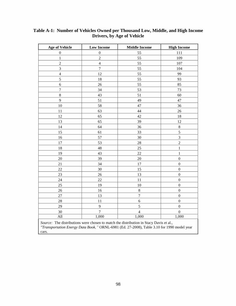
98
Table A-1: Number of Vehicles Owned per Thousand Low, Middle, and High Income
Drivers, by Age of Vehicle
Age of Vehicle Low Income Middle Income High Income
0 0 55 111
1 2 55 109
2 4 55 107
3 7 55 104
4 12 55 99
5 18 55 93
6 26 55 85
7 34 53 73
8 43 51 60
9 51 49 47
10 58 47 36
11 63 44 26
12 65 42 18
13 65 39 12
14 64 36 8
15 61 33 5
16 57 30 3
17 53 28 2
18 48 25 1
19 43 22 1
20 39 20 0
21 34 17 0
22 30 15 0
23 26 13 0
24 22 11 0
25 19 10 0
26 16 8 0
27 13 7 0
28 11 6 0
29 9 5 0
30 7 4 0
All 1,000 1,000 1,000
Source: The distributions were chosen to match the distribution in Stacy Davis et al.,
"Transportation Energy Data Book,” ORNL-6981 (Ed. 27-2008), Table 3.10 for 1990 model year
cars.

99
A.2 Driver Utility Function, R
jtU
Drivers measure the net utility of hydrogen vehicles, R
jtU , as the utility of a hydrogen
vehicle minus the utility of a non-hydrogen vehicle using the following equation:
R S V F
jt t jt jt j jt jtU P P P T I W (A.1)
where:
S
tP = the difference in price paid, or sticker price difference between hydrogen and non-
hydrogen vehicles
V
jtP = the fuel cost advantage of hydrogen vehicles over non-hydrogen vehicles;
F
jtP = agent j’s disadvantage due to limited familiarity with hydrogen vehicles
Tj = utility from a hydrogen minus that from a non-hydrogen vehicle and other things
being equal, or agent j’s taste for the hydrogen vehicle, resulting in this case from
a preference for green vehicles;
Ijt = fueling inconvenience associated with owning a hydrogen vehicle;
Wjt = worry factor associated with finding a hydrogen refueling station.
The units of each of the utility terms are dollars. When the time comes for the driver
agent to purchase a new vehicle, the utility function is used to decide whether it will be a
hydrogen or non-hydrogen vehicle. Each of the terms in the driver utility function equation
above is discussed below.
A.2.1 Sticker Price Difference, S
tP
The sticker price difference is the cost of a hydrogen vehicle minus that of a non-
hydrogen vehicle.
S f f
t t tP H G (A.2)
where;
f
tH = the average sticker price of a hydrogen-powered light-duty vehicle.
f
tG = the average sticker price of a non-hydrogen-powered light-duty vehicle;

100
Numerical values of sticker price differences used in this study are presented in Section
4.1 of the main body of the report.
A.2.2 Fuel Cost Advantage, V
jtP
V
jtP , the fuel cost advantage of hydrogen vehicles over non-hydrogen vehicles, enters the
utility function as a discounted sum of the savings on fuel costs, calculated as follows:
41 [1 ( / 4)]
*( )*/ 4
LV v g v h
jt j
rP d g e h e
r
(A.3)
where:
V
jtP = fuel cost advantage;
dj = number of miles each agent j drives each quarter;
gv = cost per gallon of gasoline;
hv = cost per kilogram of hydrogen;
eg = fuel efficiency of non-hydrogen vehicles, in gallons per mile;
eh = fuel efficiency of hydrogen vehicles, in kg per mile;
r = driver annual discount rate;
L = driver time horizon for evaluating fuel savings.
The discount rate is divided by four and the time horizon is multiplied by four to account
for the fact that the driver model operates in time intervals of quarters, not years.
The cost per unit of fuel multiplied by the units per mile yields a cost per mile of using
the fuel. The cost per mile of using non-hydrogen minus that of hydrogen is multiplied by the
number of miles driver agent j drives each period, to give quarterly fuel savings, which is then
multiplied by the capitalization factor to give the present value of fuel savings.
Additional information regarding the influence of the fuel cost advantage is presented in
Section 4.2 of the main body of the report which provides results of a sensitivity study of this
parameter.

101
A.2.3 Disadvantage Due to Limited Familiarity and Bandwagon Coefficient, F
jtP and qj
The disadvantage due to limited familiarity is calculated using a familiarity premium
equation. The familiarity premium, F
jtP , measures the dollar value of driver agent j’s familiarity
with hydrogen vehicles at time t. The rate at which the familiarity premium declines is
calculated using the bandwagon coefficient, qj.
Drivers with higher bandwagon coefficients are more inclined to imitate others. In each
period, each driver agent’s bandwagon coefficient is multiplied by the proportion of hydrogen
vehicles on the road in the previous period, and that product is subtracted from the current value
of the familiarity disadvantage, yielding a smaller disadvantage each period, which is unique to
each driver. When the familiarity disadvantage reaches zero for a driver, it cannot decrease
further and the bandwagon effect has had its maximum impact.
The familiarity premium required of agent j at time t, F
jtP , is given by:
1
0
[1 min( ( / ),1)]t
F F
jt j i
i
P q N M
(A.4)
where:
βF
= the value of full familiarity, i.e., the amount a driver who is completely unfamiliar
with a hydrogen vehicle would have to be paid to be willing to purchase the
vehicle;
Ni = the total number of hydrogen vehicles in the model area in period i;
M = the stock of vehicles in the model area, so that Ni/M is the proportion of driver
agents who already own hydrogen vehicles;
qj = the bandwagon coefficient, a multiplier that converts a given level of adoption to
an amount of familiarity gained by agent j;
βF
is the initial familiarity premium which driver agents require if they are to choose a
hydrogen vehicle over a non-hydrogen vehicle. This initial familiarity premium is common to
all drivers. Thereafter, in each period it decreases by the fraction of the vehicle stock in Los
Angeles that is hydrogen fueled, multiplied by the agent-specific scaling factor qj, the bandwagon
coefficient.
The bandwagon coefficient is distributed log-normally among the driver agents with the
mean and variance parameters of the distribution chosen such that the adoption path of the

102
hydrogen vehicles approximates the consumer goods Bass curve from the literature.50
Once it
reaches $0, the familiarity premium does not decline any more.
Additional information regarding the influence of the disadvantage due to limited
familiarity and the bandwagon effect is presented in Sections 3.2.1 and 3.2.2 of the main body of
the report, which provide results of sensitivity studies of these parameters.
A.2.4 Greenness, Tj
Each driver has a taste for greenness, and each driver agent is assigned a value from a
taste distribution. In the benchmark case, greenness values are distributed log normally among
drivers with a median of $250. Similar to the bandwagon effect, a log normal distribution
implies that the minimum level of greenness is $0. Most drivers cluster at similar, low values,
with a minority of drivers having very high values. The minimum is $0 taste for greenness,
assuming that a vehicle with no pollution would at worst have no positive effect on a person’s
purchase decision.
In the utility function, Tj is agent j’s intrinsic taste for the hydrogen vehicle resulting
from a preference for a green vehicle. Tj is also measured in dollars and is added to the driver’s
utility, so that if agent j is otherwise indifferent between hydrogen and non-hydrogen vehicles
but is willing to pay $100 for the environmental benefits of a hydrogen vehicle, Tj equals 100.
Additional information regarding the influence of greenness is presented in Section 3.2.3
of the main body of the report which provides results of a sensitivity study of this parameter.
A.2.5 Inconvenience, Ijt
Driver agent j’s inconvenience in period t is measured in dollars and is given by the
following equation:
VIIIIII w
jt
g
jt
e
jt
s
jt
n
jtjt *)( (A.5)
where:
Ijt = total inconvenience experienced by the driver;
n
jtI = inconvenience from not being able to make a trip with a hydrogen vehicle;
50 The benchmark values used is from the average imitation and innovation parameters from 213 applications in 15 separate
articles summarized in Frank M. Bass, Trichy V. Krishnan, and Dipak C. Jain, ―Why the Bass Model Fits without Decision
Variables,‖ Marketing Science 13 (1994), Table 2, p. 214; The high and low values are taken from estimates of imitation and
innovation in the diffusion of color television, clothes driers, and room air conditioners, with color television diffusion
representing low bandwagoning and with clothes dryer diffusion representing high bandwagoning. Fareena Sultan, John U.
Farley, and Donald R. Lehmann, ―A Meta-Analysis of Applications of Diffusion Models,‖ Journal of Marketing Research 27
(1990), Table 2, p. 75.

103
s
jtI = inconvenience from having to make a special trip to buy hydrogen;
e
jtI = inconvenience from having to buy hydrogen earlier than desired;
g
jtI = inconvenience from finding a hydrogen station supply exhausted and having to
travel to another;
w
jtI = inconvenience from finding a hydrogen station supply exhausted and waiting for
more supply;
V = the present value multiplier that allows the driver to take into account expected
inconvenience over the entire life of the vehicle.
Each of these inconvenience terms is the total inconvenience incurred over the course of
the quarter from all of the times each of these events occurs. They are all measured in dollars.
The following paragraphs present in detail the various sources of inconvenience to the
driver.
Not being able to make a trip. When an agent cannot make a trip with a hydrogen
vehicle, a base inconvenience cost is incurred for the loss of that trip as well as additional
inconvenience based on its length. The term n
jtI is the sum of all these occurrences in a given
quarter:
1
( )T
n nf nv n
jt a
a
I i i d
(A.6)
where inf
is the base inconvenience cost associated with not being able to make a trip with a
hydrogen car, inv
is the inconvenience cost incurred per mile of the trip the agent could not take,
and n
ad is the length, in miles, of the ath
trip the driver agent must give up this quarter. T
represents the total number of trips the driver owning a hydrogen vehicle would have to forgo
this quarter.
Having to make a special trip. As with forgone trips, each special trip an agent must
make causes him to incur a base inconvenience cost and additional inconvenience costs based on
the trip’s length. The term s
jtI is the sum of all these occurrences in a given quarter:
1
( )T
s sf sv s
jt a
a
I i i d
(A.7)
where isf is the base inconvenience cost associated with needing to make a special trip, i
sv is the
inconvenience cost incurred per mile of that trip, and s
ad is the length, in miles, of the ath
special

104
trip the driver agent must make this quarter. T represents the total number of special trips the
driver owning a hydrogen vehicle would have to make this quarter.
Having to refuel earlier than desired. Each time an agent has to buy fuel earlier than
desired because of a scarcity of hydrogen fueling sites, a cost per mile is incurred based on how
much later, in miles, refueling would have been wanted. The term Iejt is the sum of all these
occurrences in a given quarter:
1
( )T
e ev e
jt a
a
I i d
(A.8)
where iev
is the inconvenience cost incurred per mile, and e
ad is the distance, in miles, to the
point the driver would have preferred to refuel at on the ath
occurrence of an early refueling. T
represents the total number of times the driver needs to refuel early in a quarter.
Finding a station over capacity. Each time an agent finds a station at overcapacity, a
one-time inconvenience cost is incurred. The term g
jtI is the sum of all these occurrences in a
given quarter:
1
1T
g op
jt
a
Total Sales inCellI i
Capacity of Cell
(A.9)
where igf
is the inconvenience cost associated waiting in a queue, iop
reflects the inconvenience
cost of refueling at a station that is 100% over-capacity, and T represents the total number of
times that happens to this agent this quarter.
Present value term. The present value term V multiplied by this quarter’s
inconvenience cost gives the full discounted cost of inconvenience over the driver time horizon.
The present value term is given by the following equation:
41 [1 ( / 4)]
/ 4
LrV
r
(A.10)
where:
r = the annual discount rate;
L = driver time horizon.
A.2.6 Worry, Wjt
Worry is accumulated each time a driver refuels when the tank is between the ―want-to-
buy‖ and ―desperate-to-buy‖ points. For example, if the want-to-buy point is when the tank is

105
20% full and the desperate-to-buy point is when it is 5% full, then refueling after depleting more
than 80% of the tank causes worry. A driver will never make a trip that depletes more than 95%
of the tank. Worry increases nonlinearly in distance from the optimal-to-refuel point.
Driver agent j’s worry in quarter t is measured in dollars and is given by the following
equation:
1
1
* * (1 )T
jt
a
fW V w
h
(A.11)
where:
V = The present value multiplier that allows the driver to take into account how
much worry is expected over the entire life of the vehicle. This is the same as the
multiplier for inconvenience.
w = The most a driver can worry, measured in dollars. Worry reaches this level when
the amount of fuel in the tank reaches the desperate-to-buy level;
f = The amount of fuel left in the tank above the desperate-to-buy level, measured in
hundred-thousandths of a tank of fuel;
h = The amount of fuel left in the tank above the desperate-to-buy level at which
worry reaches one-half its maximum, measured in hundred-thousandths of a tank
of fuel; this parameter allows the user to choose the rate at which worry grows;
T = The total number of times the driver agent gets worried this quarter, which is
basically the total number of times the driver actually makes a trip and refuels
after the fuel tank has passed the ―want-to-buy‖ point.
A.3 Refueling
To carry out the above calculations of worry and inconvenience requires knowing 1)
where agents travel (travel behavior) and 2) how they prefer to refuel (refueling behavior). In
general, driver agents will incur less inconvenience and worry as the number of hydrogen
stations increases, especially along the travel route of the driver.
Section A.3.1 presents an explanation of trip routes taken by driver agents. Discussions
regarding how driver agents make decisions about refueling are presented in Sections A.3.2, and
A.3.3.
A.3.1 Trip Routes
Each driver agent travels on a certain number of commuting and non-commuting routes
each quarter. The commuting trips are between home and work locations. Non-commuting trips

106
are between home and non-work locations such as regional attractions, shopping malls, and so
on. Depending on the home location, there are 20 possible trip routes outside of a work
commute that a driver can take. From this individual set of trips for a driver, 20 trips are
randomly selected with replacement each quarter. Consequently, it is possible that in one quarter
a driver would happen to be assigned relatively longer non-commute trips from the set of
possible trips, and in another quarter would be assigned relatively shorter trips. This gives rise to
variation in the driving distance of drivers to reflect a similar stochastic element in real world
driving behavior.
For the purpose of simulation, all the trips are intertwined in a larger trip called a
megatrip. The megatrip is what the drivers undertake each quarter of a simulation. Since the
length of a megatrip need not necessarily approximate the annual driving range of 12,000 miles,
a multiplier is applied to actual length of the megatrip to scale it up. This multiplier is calculated
only in the first year of simulation and equals 12,000/actual length of the megatrip. The
multiplier assigned during this first period stays with the driver agent for the entire run of the
model. So when the driver is designated the trips in the first year and the trips total 6,000 miles,
the multiplier will be 2, and the total miles driven will be 12,000. The next year, if the driver
receives trips assigned that add to 7,000 miles, total miles driven will be 14,000 the following
year.
A.3.2 Refueling Decision
All drivers have the following three salient markers on their fuel gauge, though the precise
level of these markers may differ from driver to driver.
Willing-to-buy level;
Want-to-buy level;
Desperate-to-buy level.
In the model, a driver agent loses fuel at a varying rate depending on the cells (highway
or local, diagonal or straight road) being traversed, and must eventually refuel. The driver would
prefer to buy fuel as close to the want-to-buy level as possible but no sooner than the willing-to-
buy level. If the driver is unable to buy fuel and indeed hits the want-to-buy marker on the fuel
gauge, inconvenience begins to register. Thus, hitting the want-to-buy level on the fuel gauge is
an inconvenience event. If the driver is still not able to buy fuel even after hitting the want-to-
buy level, worry would also start accumulating. Worry will be accumulated between the want-
to-buy level and the desperate-to-buy level.
The case of a driver not being able to refuel is not permitted in the model. It is assumed
that all drivers are assumed to possess a GPS device that gives them locations of each hydrogen
fuel station. If they would not be able to refuel on the way, they would first consider topping-off
their tanks by making special trips to the nearest hydrogen fuel station, and would then undertake
their regular trips. When the drivers have to do this, they incur a penalty to reflect the time and
money cost of such a special refueling trip. If the nearest hydrogen fuel station is so far away
that the driver would lose enough fuel on the way back to again make the planned trip unfeasible

107
then the driver foregoes the planned trip and incurs a penalty to reflect the value of the foregone
trip.
Since each agent represents some 1,000 vehicles, even if not all these vehicles are
hydrogen vehicles, the choice of which hydrogen fuel station from which to purchase fuel has a
significant effect on a hydrogen fuel station’s total sales. This fact, coupled with the limited
selection of trips each agent can make, means that it is not unlikely that a single hydrogen fuel
station might receive a large proportion of the driver’s purchases to the exclusion of other
hydrogen fuel stations in the immediate vicinity. Drivers traveling the same routes, even from
the same starting point, will spread out their purchases over all the hydrogen fuel stations in the
vicinity. This concern is taken into account in two ways. Since there can be many hydrogen fuel
stations in a single cell, a purchase made at a given cell is divided evenly among all hydrogen
fuel stations in that cell. Secondly, if there are other cells containing hydrogen fuel stations
within an exogenous input driving distance of that cell, then the purchase is first divided evenly
among all such cells, then within each cell, among the hydrogen fuel stations in that cell.
A.3.3 How Much Hydrogen Fuel to Buy
Whenever driver agents stop to refuel, they top off their tanks so that the fuel purchased
is equal to the maximum tank capacity minus current fuel level. If all the vehicles in a driver
agent’s fleet were driven the same number of miles, this would be sufficient. However, it is
assumed that newer vehicles are driven more than older vehicles, so a weighting factor that takes
into account the ages of the hydrogen vehicles in the driver agent’s fleet is used to determine the
purchase of hydrogen.
When a driver agent stops at a hydrogen fuel station to refuel, only that weighted
proportion, which could be zero, of the total purchase is credited to the hydrogen fuel stations
from which the purchase has been made.

108
APPENDIX B: INVESTOR MODULE
B.1 Price Charged for Hydrogen Fuel
B.2 Station Siting
B.2.1 Forecasting Expected Hydrogen Fuel Sales
B.2.1.1 Unadjusted Sales at a Location, *
, 1j tD
B.2.1.2 Adjustments for Sales to Stations Planned but Not Yet Operational, **
, 1j tD
B.2.1.3 Estimation of the Growth Parameter, Gt
B.2.1.4 Estimating Future Sales Using a Logistic Growth Function, , 1j t sD
B.2.1.5 Estimating Future Sales Using a Simpler Approach
B.2.2 Effect of a New Station on Profitability of Entire Set of Stations
B.2.2.1 Net Present Value (NPV) Calculations
B.2.2.2 Ranking of Locations
B.2.2.3 Net Present Value (NPV) Rule for Station Siting
B.3 Number of Investors
B.3.1 Single Investor
B.3.2 More than One Investor
B.4 Options beyond Runs in this Study
B.4.1 Using Current Capacity Utilization to Rank Locations
B.4.2 Allowing the Investor to Be a Loss Leader in Siting Stations
B.4.3 Introducing a Capital Budget Constraint in the Investor’s Decision-Making

109
B.1 Price Charged for Hydrogen Fuel
The price charged for hydrogen fuel is set to equal the average cost of producing
hydrogen, derived from H2A, plus any tax. The price charged by the investor for hydrogen fuel,
P, is then given by:
A rC
P U EH
(B.1)
where:
U = per kilogram variable cost of hydrogen;
E = per kilogram tax on hydrogen fuel;
A = annual maintenance costs inclusive of any depreciation and interest payment on
borrowed funds;
C = equity’s share of capital costs;
r = rate of return on equity;
H = effective capacity of the station in kg/year51
; and,
= expected capacity utilization of the plant.
Table 3-1 of the study provides the price of hydrogen fuel used in the benchmark run of
the model.
B.2 Station Siting
B.2.1 Forecasting Expected Hydrogen Fuel Sales
In order to decide whether to invest in another fueling station, the investor makes a
forecast of future sales at each location in the city. This forecast is made by employing a logistic
growth function. The logistic growth function requires knowing the most recently completed
year’s sales (base sales), the sales corresponding to the entire target population adopting the
innovation (saturation sales), the rate of growth parameter.
The investor estimates base sales in two steps. First, as explained in Section B.2.1.1
below, ―Unadjusted Sales at a location,*
, 1j tD ,‖ the most recently completed year’s sales at the
location are observed using the data supplied by the driver module run for the previous year. In
51 Dispensing forecourts of centralized plants and distributed stations have the same nameplate capacity of 1,500 kg/day.

110
the second step, the investor adjusts the most recently completed year’s sales at this location by
the diversion of sales, if any, to newly planned stations near the location under consideration.
This adjustment process is described in Section B.2.1.2 below, ―Adjustments for Sales to
Stations Planned but Not Yet Operational, **
, 1j tD .‖ When the adjustment is made, the investor has
an estimate of this location’s base sales which can be used to forecast future sales at that
location.
Saturation sales are based on the assumption that by the time sales reach the maximum
possible level at any location, there would be at least one fueling station at all possible station
locations. For this reason, the saturation level of hydrogen sales is obtained in a pre-run of the
simulation in which all the vehicles are hydrogen and all the locations have fueling stations.
The growth parameter is developed using a Bayesian learning algorithm. Section B.2.1.3
below, ―Estimation of the Growth Parameter, Gt,‖ provides additional details.
Estimates of fuel sales are developed applying the logistic growth function as described
in Section B.2.1.4 below, ―Estimating Current and Future Year Sales at a Location Using a
Logistic Growth Function, , 1j t sD .‖
B.2.1.1 Unadjusted Sales at a Location, *
, 1j tD
The investor is able to observe directly the most recently completed year’s hydrogen
sales at the locations where a fueling station existed during the previous year. For such
locations, the estimate of the most recently completed year’s sales are the fuel sales that were
observed in the previous year, i.e.,
*
, 1 , 1j t j tD S (B.2)
where
*
, 1j tD = the investor’s estimate of base sales at each location j that had at least one
fueling station in the most recently completed year;
, 1j tS = the realized sales at location j in the most recently completed year.
Fuel sales at the locations where no station existed in the previous year are zero by
definition, but the investor must estimate of how much fuel may be expected to be sold at these
locations, if stations were to be sited there. These estimates are made using a regression that
relates fuel sales in a location to the vehicle traffic passing through the location and to
competition from nearby fueling stations. The regression is:
, 1
0 , 1
1, 1
Ni t i
n n t i
ni t
Sa a C
V
(B.3)

111
where:
Si,t-1 = fuel sales in grid cell i in the year t-1;
Vi,t-1 = vehicle traffic passing through location i in the year t-1;
a0 = constant term;
, 1
i
n tC = the count of locations in the nth
ring around location i which had at least one
station in the last period; the investor counts the number of cells with a fuel
station in each of several rings around the candidate location; the number of rings
(up to 3) and their radii are exogenous input parameters; if the investor chooses to
ignore the surrounding rings in the regression estimation (i.e., choosing N = 0),
then only the average sales/traffic ratio is used to predict base sales volume;
an = regression coefficient;
i = error term.
Denoting the estimated coefficients by 0a
, 1a
, and na
, the investor estimates base sales for
locations without any station in the previous period as:
*0, 1 , 1 , 1
1
Nj
nj t j t n t
n
D V a a C
. (B.4)
Putting the previous two equations together, and using Kj,t-1 to denote the number of
stations that existed in location j in the most recently completed year, the investor’s estimate of
the previous year’s sales in location j is:
, 1 , 1
*
, 10, 1 , 1 , 1
1
0
10
l t j t
Nj t j
nj t n t j t
n
S if K
D for j to LV a a C if K
. (B.5)
The regression in equation (B.3) was based on observing all vehicle traffic. As a variant
considered in the sensitivity analysis in Section 3.3.4 of the main body of the report, ― First Year
Demand Estimation at Potential Station Locations,‖ the investor could focus on hydrogen vehicle
traffic only, not simply all vehicle traffic. Using this method entails a redefinition of Vi,t-1 in
Equation (B.3) to refer to hydrogen vehicle traffic only.

112
B.2.1.2 Adjustments for Sales to Stations Planned
But Not Yet Operational, **
, 1j tD
The estimate of the most recently completed year’s sales in Equation (B.5) gives base
sales before the investor has decided to site any new stations. When a first station is established
at a location that previously did not have one, that station is able to attract some of the fuel sales
that would have taken place otherwise at nearby locations. The estimates of fuel sales in the
nearby locations must be adjusted to allow for this diversion effect. The adjustment is:
, 1
** * 1 2
, 1 , 1 0
1 1
nl tj
N L
j t j t K nln l
D D I I a
(B.6)
where
**
, 1j tD = the adjusted expected base sales at location j, taking into consideration any
diversion effect of planned stations;
*
, 1j tD = the unadjusted estimate of the most recently completed year’s sales.
To define ―nearby,‖ the investor considers N surrounding rings, leading the first
summation in Equation (B.6) to be over n =1 to N. The estimated diversion effect of a location
newly populated with a fuel station is na
. This estimate is obtained from the regression defined
in Equation (B.3). For each ring, the investor iterates over all the locations, obtaining a negative
effect specific to that ring for each location that meets two criteria:
The location must lie in the one of the surrounding rings of the location j.
Using n
j to denote the n
th ring around the location j, this condition is captured
by the first indicator function, 1njl
I
;
The location must be getting its first station under the station siting plan of the
current year. This condition is captured by the second indicator function,
, 1
2
0l tKI .
Given that each planned station can potentially cause a diversion of sales, the adjustment
needs to be calculated for each potential new station evaluated.
B.2.1.3 Estimation of the Growth Parameter, Gt
The investor’s estimate of the rate of growth of sales at each station is this year’s minus
last year’s area-wide sales. In the benchmark case from which sensitivity is explored, the
investor’s Gt is 30% for the first and second years. Beginning with the third year, the investor
applies Bayesian inference in connection with the observed rate of growth in sales between the

113
preceding two years to update the previous estimate Gt. The new estimate is a weighted average
of the previous growth estimate, or ―prior,‖ and the observed growth rate. The weights reflect
the rapidity with which the investor learns from experience. The larger the weight on the most
recent observation, the faster is learning. The equation for Gt is:
0
1 ,
2
(1 ) 2t obs
t t l
G if tG
w G wG if t
(B.7)
where
Gt-1 = the most recently completed year’s estimate of growth, also known
as the prior;
w = Bayesian weight on the most recent observation;
,
obs
t lG = the average of observed growth rates in the past, i.e.,
1
1
21
1 _
1
21
tobs
t
S SG
t SS
D
(B.8)
D = the maximum sales potential of the model area; and,
S = hydrogen sales in period .
B.2.1.4 Estimating Future Sales Using a Logistic Growth Function, , 1j t sD
Having obtained adjusted base sales and the estimated growth parameter, the investor
uses a logistic growth function assuming that the upper bound on sales is the vehicle stock of the
region: _
**
, 1
, 1 _**
, 1
exp( ) for 1 to
[exp( ) 1]
j j t t
j t s P
j j t t
v D D sGD s T
v D D sG
(B.9)
where **
, 1j tD = adjusted base sales at location j;
D = model area hydrogen sales if all vehicles used hydrogen;
jv = the sales share of location j in D ;

114
TP = planning horizon of the investor. Investor estimates sales
over the next Tp years.
An illustration of the sales forecast made by investors is shown in Figure B-1. Initially
sales grow slowly, driven by early adopters who are relatively few in number. As information
about performance increases as abetted by observing successful experience of those who have
adopted, more drivers adopt. The process feeds on itself, further speeding up adoption, until
there are fewer non-adopters remaining. With fewer drivers remaining to be convinced, the
growth in percentage of all drivers adopting in any year slows down.
Figure B-1: Logistic Growth Function
0.0
0.2
0.4
0.6
0.8
1.0
1 6 11 16 21 26 31 36
Year
Sa
les
B.2.1.5 Estimating Future Sales Using a Simpler Approach
An alternative to assuming the investor uses a logistic forecast of sales is to assume the
investor forecasts sales to grow for one period only and then stabilize. This case is considered in
Section 3.3.5 of the main body of the report, ―Expectation of Growth,‖ exploring sensitivity of
growth of hydrogen sales to investor method of forecasting sales. In this case, the estimate of
growth is:
1 2
2
obs t tt
t
S Sg
S
. (B.10)

115
Equation (B.9) in Section B.2.1.4 ―Estimating Future Sales Using Logistic Growth
Function, , 1j t sD ,‖ is replaced by:
**
, 1 , 1(1 ) 1j t s j t t PD D g for s toT (B.11)
B.2.2 Effect of a New Station on Profitability of Entire Set of Stations
Beyond being concerned with the profits from sales at a new station, the investor is
concerned with the profitability of the entire set of stations at all locations as determined by how
the addition of a new station at one of those locations will affect the profitability of all stations at
all locations.
B.2.2.1 Net Present Value (NPV) Calculations
To accurately reflect profitability, net present value (NPV) calculations are needed taking
account of cash inflows and outflows. Cash inflows come from revenues realized from the sale
of hydrogen. Cash outflows include capital outlays in establishing new stations and periodically
replacing major components such as compressor systems, annual maintenance and other
recurring expenditures including feedstock, plus over-capacity penalties incurred when sales at a
station exceed the regular capacity of the station, e.g., when customers are supplied using
hydrogen trucked-in from other fueling stations or industrial facilities.
To estimate the impact of an additional station on the NPV of the set of stations, the
investor first calculates the value of the set of stations without the additional station (i.e., the
default value), and then the value of the set of stations with the proposed station. Finally, the
value of waiting is calculated, i.e., the value of the set of stations if another year were to pass
before building a station.
The default NPV is calculated as follows:
0
, 1
1 1
, 1 , 1
, 1
(1 )
( ) min , ( ) max ,0
PT Ls
l t s l
s l
l t s l t s
l t s l
l l
NPV r K A
where
D DK P U H P V H
K K
(B.12)
where
, 1l t sD = Investor’s estimate of sales at location l in future year t+s-1. This estimate is
obtained in Equation (B.9) or alternatively (B.11) above;
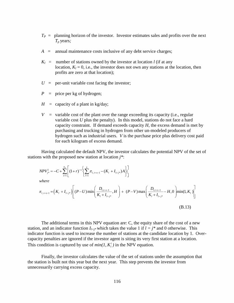
116
TP = planning horizon of the investor. Investor estimates sales and profits over the next
Tp years;
A = annual maintenance costs inclusive of any debt service charges;
Kl = number of stations owned by the investor at location l (if at any
location, Kl = 0, i.e., the investor does not own any stations at the location, then
profits are zero at that location);
U = per-unit variable cost facing the investor;
P = price per kg of hydrogen;
H = capacity of a plant in kg/day;
V = variable cost of the plant over the range exceeding its capacity (i.e., regular
variable cost U plus the penalty). In this model, stations do not face a hard
capacity constraint. If demand exceeds capacity H, the excess demand is met by
purchasing and trucking in hydrogen from other un-modeled producers of
hydrogen such as industrial users. V is the purchase price plus delivery cost paid
for each kilogram of excess demand.
Having calculated the default NPV, the investor calculates the potential NPV of the set of
stations with the proposed new station at location j*:
1
* , 1 *
1 1
, 1 , 1
, 1 *
* *
(1 ) ( )
( ) min , ( ) max ,0 min(1, )
PT Ls
j l t s l l j
s l
l t s l t s
l t s l l j l
l l j l l j
NPV C r K I A
where
D DK I P U H P V H K
K I K I
(B.13)
The additional terms in this NPV equation are: C, the equity share of the cost of a new
station, and an indicator function Il=j* which takes the value 1 if l = j* and 0 otherwise. This
indicator function is used to increase the number of stations at the candidate location by 1. Over-
capacity penalties are ignored if the investor agent is siting its very first station at a location.
This condition is captured by use of min(1, i
lK ) in the NPV equation.
Finally, the investor calculates the value of the set of stations under the assumption that
the station is built not this year but the next year. This step prevents the investor from
unnecessarily carrying excess capacity.

117
2
* , 1 *
1 1
, 1 , 1
, 1 * 1
* 1 * 1
(1 ) ( )1
( ) min , ( ) max ,0 min(1, )
PT Ls
j l t s l l j
s l
l t s l t s
l t s l l j s l
l l j s l l j s
CNPV r K I A
r
where
D DK I I P U H P V H K
K I I K I I
(B.14)
The additional term in the equation above is the indicator function Is>1 which is 1 if s > 1
and 0 otherwise. This indicator function allows the investor to estimate the effect of siting the
station at this location not in the current year but the next year.
B.2.2.2 Ranking of Locations
In order to select a candidate station, the investor needs to rank all the locations in order
of their profitability with a new station. Ideally, the investor should reorder the locations every
time a decision is made to add a new station, in case locating a new station at one location affects
the profitability of existing stations at other locations. However, in a case of approximative
behavior considered here, the investor ranks the locations only once a year. At the beginning of
each year, the investor calculates the increase in the NPV of the set of stations by adding one
more station. This additional station is alternatively placed at each of the possible locations.
The resulting NPV, when compared to NPVs obtained by placing stations at other locations,
determines the rank of that location:
(B.15)
In this equation, N is the total number of locations where fuel stations can
be sited, and NPVi is the NPV of the investor’s portfolio with an additional station at location i.
* j lNPV NPVI is an indicator function that has a value of 1 if NPVJ* ≥ NPVl, and is 0 otherwise.
B.2.2.3 Net Present Value (NPV) Rule for Station Siting
Once the ranking of locations is completed, the investor applies an NPV rule for siting
new stations to each location, in order of the location’s ranking. A new station is added if
1. The investor can increase the value of the set of stations by siting another station,
1 0
*jNPV NPV (B.16)
*
1
( *) NPV NPVj l
N
l
Rank j I

118
2. The increase in the value of the investor’s set of station by siting the station in this year is
greater than the increase expected by waiting another year to site the station,
1 2
* *j jNPV NPV (B.17)
This rule is applied for the first proposed station at the most highly ranked location, then
if that station is evaluated as profitable, for a second station at the same location, and so on until
a proposed station at that location is found to be not profitable to build this year. Then the same
sets of calculations are applied to a new station at the second-ranked location, and so on across
all 156 locations.
B.3 Number of Investors
The model’s simulations have been executed primarily with a single investor agent,
although the model can simulate the actions of multiple investors.
B.3.1 Single Investor
The case of the single investor described so far models a large corporation making
decisions about providing hydrogen infrastructure. Any market power that might be possessed
by a single investor is assumed to be of second-order magnitude and fleeting. The single
investor competes against fuel producers who supply fuel for non-hydrogen vehicles that
compete against hydrogen vehicles. Additionally, the potential entry of other large investors,
should the hydrogen price stray too high, would also constrain the single investor’s hydrogen
price. If these threats of potential competition are not sufficient, rate-of-return regulation might
occur, whose purpose is to ensure competitive-like behavior.
B.3.2 More than One Investor
This case was described in Section 3.3.6 of the main body of the report, ―Number of
Investors.‖ An investor first evaluates projects as if no other investors exist and, second, sites
stations at profitable locations taking into account the actions of other investors. Each investor
believes that all investors will act in a similar fashion, placing a station at each profitable
location with probability equal to one over the number of investors.
B.4 Options beyond Runs in this Study
This appendix has described the methods used in the simulations presented in the study.
The model can be extended to encompass many other situations. Some of these situations are
described below.

119
B.4.1 Using Current Capacity Utilization to Rank Locations
Section B.2.2.2, ―Ranking of Locations,‖ described how the investor agent ranks
locations. The rank of a location determines the order in which an investor agent will consider
siting the next station at various locations. It is also possible for the investor agent to use a
simpler rule for ranking locations in which locations are ranked simply in the order of expected
capacity utilization taking into account the proposed station. If the investor were to use this
method, Equation (B.15) above would be replaced by the following equation:
,,
1 1 , 1, 11
( ) DD j tl t
K K j tl t
N
l
Rank j I
(B.18)
In this equation N is the total number of possible locations in the model area. Di,t is
estimated fuel sales at location i in the current period as estimated in Section B.2.1.4
―Estimating Future Sales Using the Logistic Growth Function,‖ using Equation (B.9), and Ki,t-1 is
the number of stations at location i, where i = l, j in the most recently completed year. The
indicator function I( ) takes the value of 1 if ,,
, 1 , 11 1
j tl t
l t j t
DD
K K
, and 0 otherwise.
B.4.2 Allowing the Investor to Be a Loss Leader in Siting Stations
Section B.2.2.3, ―Net Present Value (NPV) Rule for Station Siting,‖ described the NPV
decision rule of the investor. Following this rule the investor would wait another year if delaying
the station by an additional year would add even more to the value of the portfolio of the stations
owned by the investor. However, if the investor is operating in a competitive market such that a
delay in station siting can lead to a loss of the market to a competitor, then the investor may site
the station in the current period even if the value of portfolio could be increased by waiting an
additional year. Such behavior is a form of loss leadership since the investor is incurring losses
to capture a larger share of the market before a competitor has an opportunity to do the same.
B.4.3 Introducing a Capital Budget Constraint in the Investor’s Decision-Making
Section B.2.2.3, ―Net Present Value (NPV) Rule for Station Siting,‖ described the NPV
decision rule of the investor. Under this rule the investor can continue to site stations as long as
they are expected to be profitable. However, it is possible that there is a limit on the number of
stations the investor can site in a given year due to a budget constraint imposed on these
expenditures. Accordingly, the investor considers siting a new station only if the remaining
budget is sufficient to finance it. The remaining capital budget of the investor should be
sufficient to site another station, i.e.,
1B
KC
(B.19)

120
where K is the number of stations sited by the investor in the current year so far, B is the total
capital budget for the year, and C is the capital cost of siting one station.

121
APPENDIX C: FACTORS AFFECTING FUTURE COSTS OF
PRODUCING HYDROGEN VEHICLES
C.1 Introduction
C.2 Hydrogen Vehicle Sticker Price
C.3 Technological Advances
C.4 Learning by Doing Estimates for HPVs
C.5 Returns to Scale and Scale Elasticities for HPVs
C.6 Summary

122
C.1 Introduction
This appendix considers the sources of decline in cost of producing hydrogen vehicles
that could enable them to enter the market place on a mass basis. Cost declines from three
sources are considered:
Technological advances in the production of HPVs
Learning by doing in the manufacturing of HPVs
Returns to scale in the production of HPVs
The following three sections review the literature with regard to these sources of price
decrease. This appendix ends with a summary.
C.2 Hydrogen Vehicle Sticker Price
Sticker price difference is the purchase price of an HPV minus that of a non-hydrogen
vehicle. Several projections of the price of an HPV relative to that of a non-hydrogen vehicle
have been made. For example, the International Energy Association in 2005 estimated that in
2030, an HPV will cost between $2,500 and $7,625 more than a non-hydrogen vehicle.52
RCF
and Argonne staffs reviewed other studies which collectively provide a range of estimated values
for future prices of HPVs relative to those of non-hydrogen vehicles.53, 54, 55, 56
Price difference
estimates vary from several thousand dollars less, to several thousand dollars more for an HPV
compared to a non-hydrogen vehicle. The time horizon usually extends to 2015, but also reaches
as far as 2025.
The main factor accounting for the difference in price of an HPV compared to price for a
non-hydrogen vehicle is the cost of the fuel cell. In turn, fuel cell cost estimates depend on the
state of technology at a particular time.
The agent-based model’s benchmark price of an HPV of equality with the price of a non-
hydrogen vehicle was selected using price and cost estimates found in the literature as a starting
point, and then applying the collective wisdom of RCF and Argonne staff to project a reasonable
estimate of the price difference looking out 30 to 40 years in the future, not 5, 10, or 20 years out
which some of the studies in the literature reference. As analyzed in this report, high and low
52 International Energy Association, ―Prospects for Hydrogen and Fuel Cells,‖ 2005,
http://www.iea.org/textbase/nppdf/free/2005/hydrogen2005.pdf, p. 101, Table 3.5. 53 Stephen Eaves and James Eaves, ―A Cost Comparison of Fuel-Cell and Battery Electric Vehicles,‖ Journal of Power Sources
130 (2004), pp. 208-212. 54 Sam Hawkins and Nick Hughes, ―Technological Characteristics of Hydrogen Fuel Cell Vehicles,‖ UKSHEC Social Science
Working Paper No. 22 (London: Policy Studies Institute, 2006), especially pp. 7, 13. 55 Joan M. Ogden, Robert H. Williams and Eric D. Larson, ―Toward a Hydrogen-Based Transportation System,‖ final draft
(Princeton University Center for Energy and Environmental Studies, May 8, 2001). 56 Haruki Tsuchiya and Osamu Kobayashi, ―Mass Production Cost of PEM Fuel Cell by Learning Curve,‖ International Journal
of Hydrogen Energy 29 (2004), pp. 985-990.

123
scenarios also were simulated, with the high case $6,500 more, and the low case $4,000 less than
the non-hydrogen vehicle cost.
C.3 Technological Advances
The price of an HPV is dependent on many factors, most important of which are costs of
manufacturing the glider, the electronic motor, the hydrogen storage system, and the fuel cell.
The most expensive of these components is the hydrogen fuel cell, and the main driver in the
expected price decline of hydrogen vehicles will be the corresponding decrease in fuel cell cost.
In the literature, fuel cells are often priced in dollars per kilowatt. Fuel cells for HPVs will have
a capacity between 70 and 100 kilowatts, with 80 kilowatts being the size assumed in this study.
Thus, an 80-kW fuel cell with a per-kilowatt cost of $50 will cost $4,000. Other important
components are the electric motor, control electronics, the hydrogen storage system, and the
glider which consists of the body and interior of the vehicle. While it is possible that glider cost
will be less for an HPV than for a non-hydrogen vehicle due to the removal of some of the
complexity associated with combustion engines in non-hydrogen vehicles, we assume
conservatively that glider cost is the same for hydrogen and non-hydrogen vehicles.57
Major avenues of progress in fuel cell technology involve three interrelated areas—
durability, reliability, and cost. Cost reduction of individual components has proceeded over the
past twenty years, and should continue, stemming from reductions in the costs of components:
1) polymer electrolyte membrane, also known as proton exchange membrane, or PEM; 2)
catalyst electrodes (i.e., membrane electrode assemblies, or MEA); 3) the fuel cell stack; 4) the
fuel cell processor; 5) the power conditioner; and, 6) air supply systems.58
57 David L. Greene, Paul N. Leiby, and David Bowman, Integrated Analysis of Market Transformation Scenarios with HyTrans
(Oak Ridge, Tenn.: Oak Ridge National Laboratory, June 2007), p. 13. 58 Department of Energy, ―DOE Hydrogen Program: 2008 Progress Report – Fuel Cells,‖ November, 2008, accessed September
1, 2009 at http://www.hydrogen.energy.gov/annual_progress08_fuelcells.html.
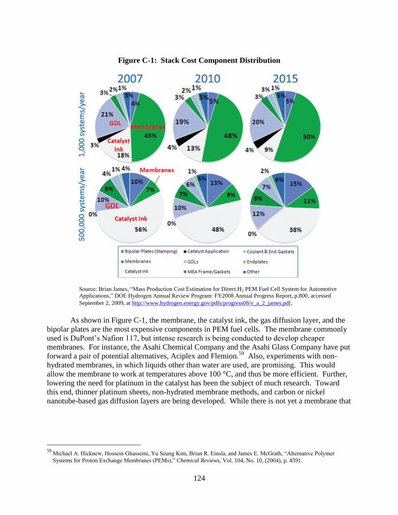
124
Figure C-1: Stack Cost Component Distribution
Source: Brian James, ―Mass Production Cost Estimation for Direct H2 PEM Fuel Cell System for Automotive
Applications,‖ DOE Hydrogen Annual Review Program: FY2008 Annual Progress Report, p.800, accessed
September 2, 2009, at http://www.hydrogen.energy.gov/pdfs/progress08/v_a_2_james.pdf.
As shown in Figure C-1, the membrane, the catalyst ink, the gas diffusion layer, and the
bipolar plates are the most expensive components in PEM fuel cells. The membrane commonly
used is DuPont’s Nafion 117, but intense research is being conducted to develop cheaper
membranes. For instance, the Asahi Chemical Company and the Asahi Glass Company have put
forward a pair of potential alternatives, Aciplex and Flemion.59
Also, experiments with non-
hydrated membranes, in which liquids other than water are used, are promising. This would
allow the membrane to work at temperatures above 100 °C, and thus be more efficient. Further,
lowering the need for platinum in the catalyst has been the subject of much research. Toward
this end, thinner platinum sheets, non-hydrated membrane methods, and carbon or nickel
nanotube-based gas diffusion layers are being developed. While there is not yet a membrane that
59
Michael A. Hicknew, Hossein Ghassemi, Yu Seung Kim, Brian R. Einsla, and James E. McGrath, ―Alternative Polymer
Systems for Proton Exchange Membranes (PEMs),‖ Chemical Reviews, Vol. 104, No. 10, (2004), p. 4591.

125
matches the DuPont product, there is a significant push for increased efficiency and lower costs
in this area.60, 61
The cost of fuel cells could be reduced further by substituting the graphite plates with
plates of cheaper composite materials, notably metal-carbon-polymer plates.62, 63
Durability
issues are being studied intensely as well. This is a topic that is especially important for fuel
cells intended for use in motor vehicles, because such systems see great variation in conditions
such as temperature and humidity which cause stress on components. Significant improvements
have been made in this area through the introduction of new catalysts, improved catalyst support
materials, optimized electro-catalyst layer structures, enhanced flow field design, and significant
improvements in fuel cell stack and system controls.64, 65
Also, system design has received some
attention, with some progress through the heat-flow-based technique called pinch technology.66
Many advances have come through better understanding of unit cell component failures, design
optimization, and operating strategies.67
Better models of system components such as the stack,
gas humidifier, pressure swing absorber, membrane reactor, fuel cell processor, and membrane
gas separator have been introduced recently or are in progress, all of which further contribute to
the development of cheaper and more efficient components.68
The Department of Energy regularly reviews the cost and technological progress of
hydrogen storage and of fuel cells. In these and other reports in the literature, the cost per
kilowatt is reported under an assumption that fuel cells are produced at a high volume, for
instance of at least 500,000 units per year (typical automobile manufacturing volume is between
75,000 and 500,000 vehicles per factory per year).
Table C-1 reports recent cost declines. High-volume cost estimates are relevant because
the gains from economies to scale are substantial, as will be seen below in Section C.5. Over
time, technological advances have brought the estimated cost down substantially.
These advances include reduction in the amount of platinum needed in constructing the
fuel cell. The Department of Energy has had as a stated goal that the price of fuel cells be $45
60 Kamaruzzaman Sopian and Wan Ramli Wan Daud, ―Challenges and Future Developments in Proton Exchange Membrane
Fuel Cells,‖ Renewable Energy Vol.31, Issue 5, (2006), pp. 719-727. 61 Sunita Satyapal, ―Hydrogen Program Overview, 2009 DOE Hydrogen Annual Review and Vehicle Technologies Program,‖
Annual Merit Review and Peer Evaluation Meeting, May 18, 2009, accessed 7/30/2009 at
http://www.hydrogen.energy.gov/pdfs/review09/program_overview_2009_amr.pdf. 62 Jinfeng Wu, Xiao Zi Yuan, Jonathan J. Martin, Haijiang Wang, Jiujun Zhang, Jun Shen, Shaohong Wu, and Walter Merida, ―A
Review of PEM Fuel Cell Durability: Degradation Mechanisms and Mitigation Strategies,‖ Journal of Power Sources,
Vol.184, Issue 1 (15 September 2008), pp. 104-119. 63 Sopian and Wan Daud, ―Challenges and Future Developments in Proton Exchange Membrane Fuel Cells.‖ 64 Wu et al., ―A Review of PEM Fuel Cell Durability: Degradation Mechanisms and Mitigation Strategies.‖ 65 Jürgen Stumper and Charles Stone, ―Recent Advances in Fuel Cell Technology at Ballard,‖ Journal of Power Sources, Vol.
176, Issue 2 (1 February 2008), pp. 468-476. 66 C. Wallmark and P. Alvfors, ―Design of Stationary PEFC System Configurations to Meet Heat and Power Demands,‖ Journal
of Power Sources, Vol. 106, Issues 1-2 (April 2002), pp. 83–92. 67 Stumper and Stone, ―Recent Advances in Fuel Cell Technology at Ballard.‖ 68 Sopian and Wan Daud, ―Challenges and Future Developments in Proton Exchange Membrane Fuel Cells.‖

126
per kW by 2010 and $30 per kW by 2015, assuming annual HPV production volume of
500,000.69
Table C-1: Costs of Fuel Cell System, Assuming 500,000 Vehicles Produced Annually
(2015 goal is $30 /kW)
Year 2002 2006 2007 2008
Cost of Fuel
Cell System $275/kW $108/kW $94/kW $73/kW
Source: Satyapal, ―Hydrogen Program Overview, 2009 DOE Hydrogen Annual Review and Vehicle Technologies
Program,‖ p. 5.
For comparison, sticker price parity between HPV and non-hydrogen vehicles is reached
roughly when the cost of an 80-kW fuel cell approaches $40 per kW.
One estimate puts the cost of an HPV at approximately $29,147, with a cost break-out by
individual components as follows: (1) fuel cell, $23,033; (2) 3.2-kg storage tank, $2,288; and,
(3) drive train, $3,826.70
The ultimate price of the HPV thus depends mostly on the cost of the
fuel cell. The components which add the most to that cost are the platinum catalysts and bipolar
plates between cells. The bipolar plates are made largely of machined graphite sheets. Some
severely reduced cost estimates include assumptions of major technological leaps in the future,
such as elimination of bipolar plates and gaskets, or uses of a carbon-polymer composite fuel cell
which can be molded for mass-manufacturing.71
The full magnitude of cost reductions in the future will depend as well on technological
progress reducing the cost of manufacturing hydrogen fuel cells, through learning by doing in
manufacturing, as factories become more adept at the production of fuel cells, and on the size of
production runs of fuel cells being large enough to capture economies of scale.
C.4 Learning by Doing Estimates for HPVs
Learning by doing refers to cost declines as a consequence of performing tasks many
times. Learning by doing is often measured by a progress ratio. This number is the ratio of the
cost of production after cumulative production doubles, to the initial cost. A 1984 paper refers to
an often-cited finding of an average industry progress ratio equal to 80% based on a 1947
analysis of progress ratios of 118 World War II airframe models.72
If a manufactured product
has a progress ratio of 80% and the production cost is $100 to make the first 100 units, when
cumulative production reaches 200 units, the second batch of 100 units will have cost $80.
69 Satyapal, ―Hydrogen Program Overview, 2009 DOE Hydrogen Program and Vehicle Technologies Program,‖ p. 5. 70 Stephen Eaves and James Eaves, ―A Cost Comparison of Fuel-Cell and Battery Electric Vehicles,‖ Journal of Power Sources
130 (2004), pp. 208-212. 71 Hawkins and Hughes, ―Technological Characteristics of Hydrogen Fuel Cell Vehicles,‖ p. 7. 72 John M. Dutton, Annie Thomas, and John E. Butler, ―The History of Progress Functions as a Managerial Technology,‖ The
Business History Review Vol. 58, No. 2 (Summer 1984), p. 222.

127
Formally, for some product, if Cost(t) is cost at time t, d(t) is the number of doublings of
cumulative output of the product at time t, and a is the percent reduction in cost for each
doubling of cumulative output (i.e., 1-a is the progress ratio), then we have Cost(t) = Cost(0)(1-
a)d.
Table C-2 below gives estimates of progress ratios for various products. Progress ratio
estimates for hydrogen vehicles exist. Separate estimates of progress ratios for fuel cells have
been given. Japanese scientists Haruki Tsuchiya and Osamu Kobayashi reported a progress ratio
of photovoltaic cost of 82% from 1979 to 1999 in Japan, while Princeton University scientists
Joan Ogden, Robert Williams and Eric Larson estimated a progress ratio for the same product of
83%.73, 74
Beyond estimating progress ratios, Tsuchiya and Kobayashi give estimates of eventual
fuel cell stack costs between $15 per kW and $145 per kW in 2020, with a middle scenario
estimate of $38 per kW or $3,800 for a 100-kilowatt fuel cell system in 2020.75
Table C-2: Progress Ratios for Various Products
Technology Period Year 1
Production
Cumulative
Production Cost Index
Progress
Ratio Ford Model T Auto 1909-1923 15,741 8,028,992 0.290 87%
Integrated Circuits 1962-1968 4 million units 828 million units 0.047 67%
CFC Substitutes 1988-1999 100,000 tons 3,871,000 tons 0.690 93%
Scrubbers 1987-1995 65.8 GW 84.3 GW 0.941 89%
Photovoltaic Cells 1971-2000 0.1 MW 1,451.4 MW 0.042 72%
Magnetic Ballasts 1977-1993 29.4 million 629.3 million 0.897 97%
Electronic Ballasts 1986-2001 431,000 350 million units 0.277 88%
Refrigerators 1980-1998 5.1 million 126.3 million 0.556 88%
Freezers 1980-1998 1.8 million 26.1 million 0.374 78%
Clothes Washers 1980-1998 4.4 million 104.7 million 0.536 87%
Electronic Clothes
Dryer 1980-1998 2.5 million 61.0 million 0.557 88%
Gas Clothes Dryer 1980-1998 0.7 million 18.2 million 0.593 90%
Dishwasher 1980-1998 2.7 million 69.7 million 0.450 84%
Room Air
Conditioner 1980-1998 2.4 million 63.3 million 0.478 85%
Selective Window
Coatings 1992-2000 4.8 million m
2 157.4 million m
2 0.394 83%
Source: John A. Laitner and Alan H. Sanstad, ―Learning-by-Doing on Both the Demand and the Supply Sides: Implications for
Electric Utility Investments in a Heuristic Model,‖ Table 1, EXCETP Workshop, Paris, January 22-23, 2003, accessed July 31,
2008, at http://www.iea.org/dbtw-wpd/textbase/work/2003/extool-excetp6/IV-laitner.pdf.
C.5 Returns to Scale and Scale Elasticities for HPVs
Returns to scale can be calculated by looking at the scale elasticity or the cost elasticity
(which are inverses of each other, such that 1 ii ECQSE ). In this case, increasing returns to
scale are consistent with a scale elasticity greater than one or, equivalently, a cost elasticity less
73 Tsuchiya and Kobayashi, ―Mass Production Cost of PEM Fuel Cell by Learning Curve,‖ p. 990. 74 Ogden, Williams, and Larson, ―Toward a Hydrogen-Based Transportation System,‖ p. 15. 75 Tsuchiya and Kobayashi, ―Mass Production Cost of PEM Fuel Cell by Learning Curve,‖ p. 988.

128
than one. Estimates for the automobile industry find that as a factory approaches full capacity,
cost elasticity increases, and the degree of increasing returns to scale diminish. Various auto
industry studies have been carried out. It has been suggested that the cost elasticity estimate is
directly related to the size of a nation’s industry. For example, the cost elasticity estimate is
0.758 in Spain,76
0.85 in Canada, 0.91 in Germany and in the U.S., 0.98 in Japan,77
and 0.98 in
Mexico.78
Van Biesebroeck gives a wider range of estimates for the United States: 0.873 to
1.15.79
Scale elasticity is also a function of level of capacity utilization. Some research has
found evidence for this at a minimum level of output, where cost elasticity is estimated to be
0.013, significant at the 0.5% level, while at maximum level, cost elasticity is estimated to be
1.293, significant at the 10% level, with 0.758 at mean output, significant at 0.5% level.80
C.6 Summary
Table C-3 summarizes the elements of the total cost of a hydrogen vehicle: the glider,
the fuel cell, the storage tank, control electronics, and the motor, and compares them to the cost
of a non-hydrogen vehicle.
In their study of market transformation scenarios, Greene and Leiby state that glider costs
are the same across all technology types and are assumed to be a constant $20,000 over time.81
From the paper by Eaves and Eaves, a conventional drive train is derived to cost about $3,800,82
and from the International Energy Association’s study, a conventional engine is implied to cost
about $2,400,83
bringing the subtotal for these two components to $6,200. Thus, a non-hydrogen
vehicle is estimated cost around $26,200 at the present time (= $20,000 + $6,200).
The current cost of an HPV is estimated from several sources. As noted above, the glider
cost of $20,000 from Greene and Leiby is used. A fuel cell cost of $144,000 is taken from an
International Energy Association study.84
The cost of a hydrogen storage tank, control
76 Lila J. Truett and Dale B. Truett. ―The Spanish Automotive Industry: Scale Economies and Input Relationships,‖ Applied
Economics Vol. 33 (2001), p. 1508. 77 Melvyn A. Fuss and Leonard Waverman, Costs and Productivity in Automobile Production: The Challenge of Japanese
Efficiency (Cambridge: Cambridge University Press, 1992), Table 5.4, p. 122. 78 James R. Tybout and M. Daniel Westbrook, ―Trade Liberalization and the Dimensions of Efficiency Change in Mexican
Manufacturing Industries,‖ Journal of International Economics Vol..39, Issues 1-2 (August 1995), p. 70. 79 Johannes Van Biesebroeck, ―Productivity Dynamics with Technology Choice: An Application to Automobile Assembly,‖ The
Review of Economic Studies 70 (2003), p. 192. 80 Truett and Truett. ―The Spanish Automotive Industry: Scale Economies and Input Relationships,‖ p. 1508. 81 Greene, Leiby, and Bowman, Integrated Analysis of Market Transformation Scenarios with HyTrans, p. 13. 82 Eaves and Eaves, ―A Cost Comparison of Fuel-Cell and Battery Electric Vehicles,‖ p. 210. 83 International Energy Association, ―Prospects for Hydrogen and Fuel Cells,‖ p. 101, Table 3.5. 84 Ibid.

129
electronics, and an electric motor were derived from the paper by Eaves and Eaves and found to
be about $6,000.85
Thus, the total estimated current cost for an HPV is about $170,000.
We include future costs of the HPV under two different sets of assumptions. First, we
give the cost if an annual HPV volume of 500,000 vehicles is assumed. The fuel cell cost
associated with this volume found in the DOE’s 2009 progress report is $73 per kW or $5,840
for an 80-kW HPV.86
The second case gives both a range of fuel cell costs and a range of the
combined costs of fuel cell tank, control electronics, and electric motor under high future annual
HPV volume.
Table C-3: Current and Future Cost Estimates of Mid-Sized Sedan, by Component
Vehicle Costs Glider
Conventional
Engine and
Drive Train
Hydrogen
Fuel Cell
Hydrogen
Storage Tank,
Control
Electronics,
and Electric
Motor
Total
Conventional
Vehicle $20,000 81 $6,200 88, 89 - - $26,200
Hydrogen Vehicle
(today) $20,000 81 - $144,000 89 $6,000 88 $170,000
Hydrogen Vehicle (2007, if annual
volume were
500,000)
$20,000 81 - $5,840 86 $6,000 88 $31,840
Hydrogen Vehicle (future, high volume) $20,000 81 -
$1,200 -
$3,040 87
$6,000 88 -
$7,500 89
$27,200-
$30,540
Fuel cell costs range from $1,200 to $3,040,87
based on results obtained by Tsuchiya and
Kobayashi for rapid and moderate progress. Costs for hydrogen storage tank, control electronics,
and electric motor range from $6,00088
to $7,50089
, taking results derived from Eaves and Eaves,
and the International Energy Association, respectively.
Depending on the estimated cost of the fuel cell, an 80-kw fuel cell HPV could cost from
$1,000 to $4,600 more than a non-hydrogen vehicle in the future, although an HPV currently
costs over $140,000 more than a non-hydrogen vehicle today. The exact cost is not certain.
There is some promise that the cost of the electric motor, control electronics, and especially
hydrogen storage tank will decline over time.90
Moreover, the hydrogen storage tank is expected
85 Eaves and Eaves, ―A Cost Comparison of Fuel-Cell and Battery Electric Vehicles,‖ p. 210-211. 86 Satyapal, ―Hydrogen Program Overview, 2009 DOE Hydrogen Program and Vehicle Technologies Program,‖ p. 5. 87 Tsuchiya and Kobayashi, ―Mass Production Cost of PEM Fuel Cell by Learning Curve,‖ p. 990. 88 Eaves and Eaves, ―A Cost Comparison of Fuel-Cell and Battery Electric Vehicles,‖ p. 210-211. 89 International Energy Association, ―Prospects for Hydrogen and Fuel Cells,‖ p. 101, Table 3.5. 90 Sam Hawkins and Nick Hughes, ―Technological Characteristics of Hydrogen Fuel Cell Vehicles,‖ UKSHEC Social Science
Working Paper No. 22 (London: Policy Studies Institute, 2006).

130
to experience more relative cost reductions compared to other components. Further reductions
from learning by doing in electric motors and control electronics would be expected to be low
given that these technologies are not new and that there are similar components in non-hydrogen
vehicles which would be expected to experience similar cost reductions.
The final column of Table C-3 shows the resulting estimates of the future possible prices
of HPVs at unspecified dates in the future. These prices are in the vicinity of the hydrogen
vehicle prices in the scenarios of the present study.