hydrological simulation program fortran (hspf… · management of land and water resources. to meet...

i

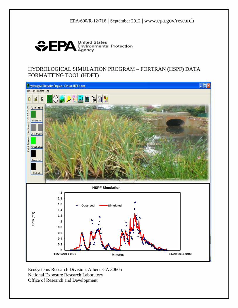
EPA/600/R-12/716 | September 2012 | www.epa.gov/research

HYDROLOGICAL SIMULATION PROGRAM – FORTRAN (HSPF) DATA

FORMATTING TOOL (HDFT)

Ecosystems Research Division, Athens GA 30605

National Exposure Research Laboratory

Office of Research and Development

0

0.2

0.4

0.6

0.8

1

1.2

1.4

1.6

1.8

2

11/28/2011 0:00 11/29/2011 0:00

Flo

w (cfs

)

Minutes

HSPF Simulation

Observed Simulated

ii

HYDROLOGICAL SIMULATION PROGRAM–FORTRAN (HSPF) DATA

FORMATTING TOOL (HDFT)

By

Mohamoud, Y.M., S. Motamarri, R. Mahajan, M. Panunto, R. Parmar,

M. Galvin, and D. Stehr

Ecosystems Research Division

National Exposure Research Laboratory


United States Environmental Protection Agency

Athens Georgia 30605

U.S. Environmental Protection Agency


Washington, DC 20460

ii

Disclaimer

This report has been reviewed by the National Exposure Research Laboratory (NERL) -

Ecosystem Research Division (ERD), U.S. Environmental Protection Agency (USEPA) in

Athens Georgia and approved for publication. Approval does not signify that the contents

necessarily reflect the views and policies of the U.S. Environmental Protection Agency, nor does

mention of trade names or commercial products constitute endorsement or recommendation for

use. Although a reasonable effort has been made to assure that the results obtained are correct,

the HSPF formatting and conversion tools described in this report may require further testing and

evaluation by developers and future HDFT users. Therefore, the author and the U.S.

Environmental Protection Agency are not responsible and assume no liability whatsoever for any

results or any use made of the results obtained from these programs, nor for any damages or

litigation that result from the use of these programs for any purpose.

Citation:

Mohamoud, Y.M., S. Motamarri, R. Mahajan, M. Panunto, R. Parmar, M. Galvin, and D. Stehr

(2012). HSPF Data Formatting Tool (HDFT). U.S. Environmental Protection Agency,

Washington, DC, EPA/600/R-12/716.

iii

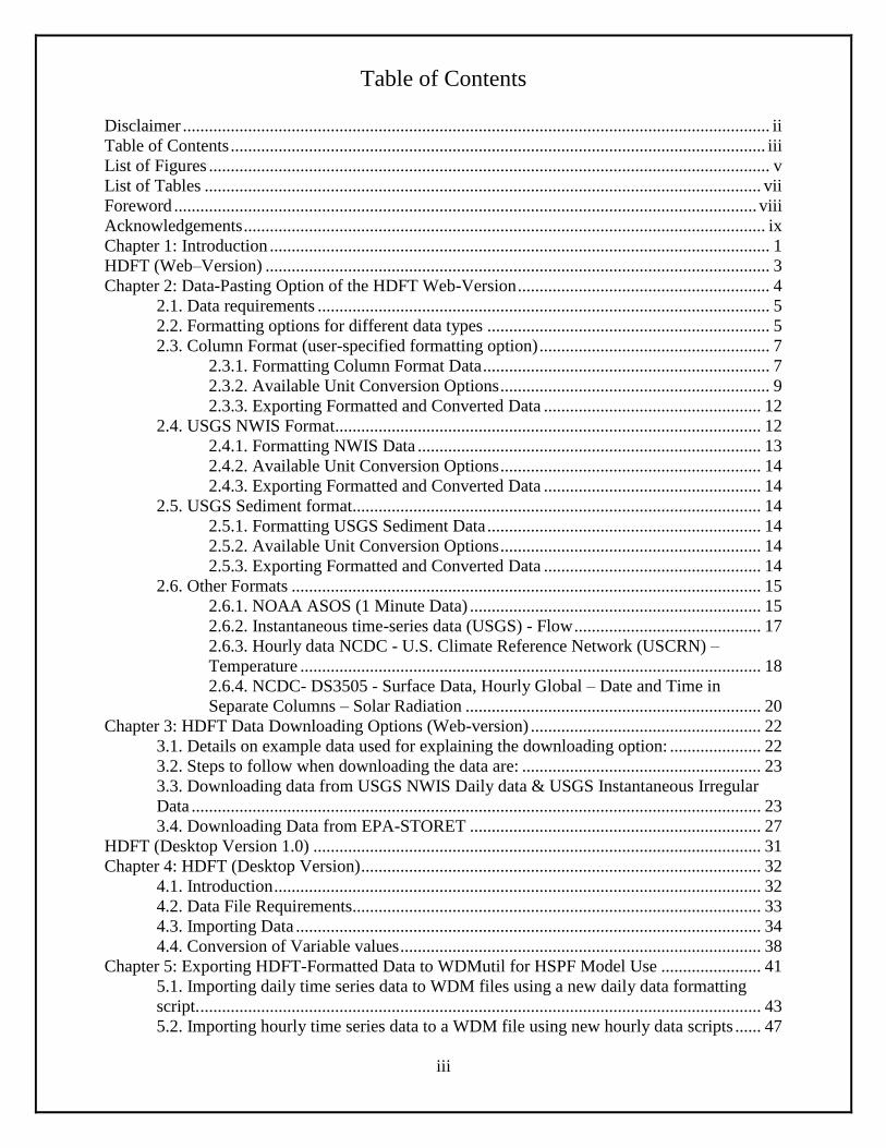
Table of Contents

Disclaimer ....................................................................................................................................... ii Table of Contents ........................................................................................................................... iii List of Figures ................................................................................................................................. v List of Tables ................................................................................................................................ vii Foreword ...................................................................................................................................... viii Acknowledgements ........................................................................................................................ ix Chapter 1: Introduction ................................................................................................................... 1 HDFT (Web–Version) .................................................................................................................... 3 Chapter 2: Data-Pasting Option of the HDFT Web-Version .......................................................... 4

2.1. Data requirements ........................................................................................................ 5 2.2. Formatting options for different data types ................................................................. 5 2.3. Column Format (user-specified formatting option) ..................................................... 7

2.3.1. Formatting Column Format Data .................................................................. 7 2.3.2. Available Unit Conversion Options .............................................................. 9 2.3.3. Exporting Formatted and Converted Data .................................................. 12

2.4. USGS NWIS Format.................................................................................................. 12 2.4.1. Formatting NWIS Data ............................................................................... 13 2.4.2. Available Unit Conversion Options ............................................................ 14 2.4.3. Exporting Formatted and Converted Data .................................................. 14

2.5. USGS Sediment format.............................................................................................. 14 2.5.1. Formatting USGS Sediment Data ............................................................... 14 2.5.2. Available Unit Conversion Options ............................................................ 14 2.5.3. Exporting Formatted and Converted Data .................................................. 14

2.6. Other Formats ............................................................................................................ 15 2.6.1. NOAA ASOS (1 Minute Data) ................................................................... 15 2.6.2. Instantaneous time-series data (USGS) - Flow ........................................... 17 2.6.3. Hourly data NCDC - U.S. Climate Reference Network (USCRN) –

Temperature .......................................................................................................... 18 2.6.4. NCDC- DS3505 - Surface Data, Hourly Global – Date and Time in

Separate Columns – Solar Radiation .................................................................... 20 Chapter 3: HDFT Data Downloading Options (Web-version) ..................................................... 22

3.1. Details on example data used for explaining the downloading option: ..................... 22 3.2. Steps to follow when downloading the data are: ....................................................... 23 3.3. Downloading data from USGS NWIS Daily data & USGS Instantaneous Irregular

Data ................................................................................................................................... 23 3.4. Downloading Data from EPA-STORET ................................................................... 27

HDFT (Desktop Version 1.0) ....................................................................................................... 31 Chapter 4: HDFT (Desktop Version) ............................................................................................ 32

4.1. Introduction ................................................................................................................ 32 4.2. Data File Requirements.............................................................................................. 33 4.3. Importing Data ........................................................................................................... 34 4.4. Conversion of Variable values ................................................................................... 38

Chapter 5: Exporting HDFT-Formatted Data to WDMutil for HSPF Model Use ....................... 41 5.1. Importing daily time series data to WDM files using a new daily data formatting

script. ................................................................................................................................. 43 5.2. Importing hourly time series data to a WDM file using new hourly data scripts ...... 47

iv

5.3. Importing sub-hourly time series data to a WDM file, using a new sub-hourly data

script .................................................................................................................................. 50 Appendix-A: Hydrological and Meteorological Variables and Unit Conversions ....................... 56 Appendix-B: Examples of Data Formats and Data Types ............................................................ 59 Appendix-C: Downloading Data from the National Climate Data Center ................................... 63 Appendix-D: STORET Data Download Options ......................................................................... 71 Appendix-E: Obtaining USGS Station Numbers .......................................................................... 81

v

List of Figures

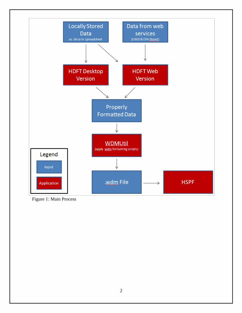
Figure 1: Main Process ................................................................................................................... 2

Figure 2: Main HDFT Window ...................................................................................................... 7 Figure 3: Enter Data Information .................................................................................................... 8 Figure 4: Import Data Window ....................................................................................................... 9 Figure 5: HDFT Main Window with Imported Data .................................................................... 10 Figure 6: Conversion of flow data from cfs to cms ..................................................................... 11

Figure 7: Conversion of imported flow data to cumulative volume ............................................. 11 Figure 8: Export Data Window ..................................................................................................... 12 Figure 9: Data Information window – USGS NWIS Format ....................................................... 13 Figure 10: Data Information window – Other Formats- ASOS .................................................... 16 Figure 11: Formatted ASOS 1 Minute data .................................................................................. 17

Figure 12: Formatted NCDC hourly climate data......................................................................... 20

Figure 13: Data Download Window ............................................................................................. 23

Figure 14: Selection of variable window ...................................................................................... 24

Figure 15: Data Download Window with Station information extracted ..................................... 25 Figure 16: Data Download Window-USGS NWIS – Entering Start and End dates .................... 26 Figure 17: Data imported using download option- USGS NWIS Daily/ Instantaneous data ....... 26

Figure 18: Data download window – EPA STORET ................................................................... 28 Figure 19: EPA STORET- Parameters available .......................................................................... 28 Figure 20: EPA STORET- Site information extracted ................................................................. 29

Figure 21: Data Download Window-EPA STORET – Entering Start and End dates .................. 30 Figure 22: Data imported from EPA STORET............................................................................. 30

Figure 23: Main Desktop Version window ................................................................................... 34 Figure 24: Import window showing the headers of the imported data file ................................... 35

Figure 25: Header window before headers were removed ........................................................... 35 Figure 26: Header window after headers were removed .............................................................. 36

Figure 27: Data ready for column identification ........................................................................... 36 Figure 28: Column identification, variable and unit selection window ........................................ 37 Figure 29: Confirmation for the date and time format .................................................................. 37

Figure 30: Columns selected for conversion and export .............................................................. 38 Figure 31: Unit conversion window ............................................................................................. 39

Figure 32: Converted flow values ................................................................................................. 39 Figure 33: Formatted data window ............................................................................................... 40 Figure 34: Name and Save the formatted data file ....................................................................... 40 Figure 35: WDMUtil Window ...................................................................................................... 42 Figure 36: An empty WDM file .................................................................................................... 43

Figure 37: HDFT exported daily flow data................................................................................... 44

Figure 38: Script for HDFT exported daily data ........................................................................... 44

Figure 39: Write daily flow data to WDM file Script for HDFT exported daily data .................. 45 Figure 40: WDM file with a single daily flow time series entry .................................................. 46 Figure 41: Examples of two different hourly formats .................................................................. 47 Figure 42: HDFT exported hourly precipitation data ................................................................... 48 Figure 43: Hourly script for HDFT formatted data ...................................................................... 48 Figure 44: Hourly precipitation data added to the WDM file ....................................................... 49 Figure 45: HDFT exported sub-hourly (5 minute interval) flow data .......................................... 50

vi

Figure 46: Sub-hourly script for HDFT formatted data ................................................................ 51 Figure 47: Change interval tab of New Time Series window ....................................................... 52

Figure 48: Change starting date for New Time Series .................................................................. 53

Figure 49: A WDM file containting three data series with daily, hourly, and sub-hourly data

resolutions ..................................................................................................................................... 54 Figure 50: Sample data to be pasted inside the tool (excluding headers) ..................................... 59 Figure 51: Column format –Sample data ...................................................................................... 59 Figure 52: USGS NWIS- Sample Data with a header .................................................................. 59 Figure 53: USGS Sediment –Sample data with a header ............................................................. 60

Figure 54: ASOS –Sample data with no header ........................................................................... 60 Figure 55: USGS instantaneous time series data – flow with a header ........................................ 61 Figure 56: NCDC - U.S. Climate Reference Network data (hourly) with a header ..................... 61 Figure 57: Sample streamflow data (with no date and time separators) - USGS Instantaneous

Data Archive format ..................................................................................................................... 62

Figure 58: NCDC – Surface data, Hourly Global data, Date and Time in separate columns ....... 62

Figure 59: National Climatic Data Center home page .................................................................. 63

Figure 60: Interactive map application page ................................................................................. 64 Figure 61: Map Help window ....................................................................................................... 64 Figure 62: GIS Map window ........................................................................................................ 65 Figure 63: Layers sub window ...................................................................................................... 66

Figure 64: Feature selection .......................................................................................................... 67 Figure 65: Results window ........................................................................................................... 67

Figure 66: Data Access Option Window ...................................................................................... 68 Figure 67: Parameter Selection window ....................................................................................... 69 Figure 68: Selection of dates and data download ......................................................................... 70

Figure 69: HDFT Data Download Window.................................................................................. 71 Figure 70: MyWATERS Mapper Welcome Page ........................................................................ 72

Figure 71: Introductory sheet ........................................................................................................ 72

Figure 72: HUC 8 watershed map. ............................................................................................... 73

Figure 73: Information about selected HUC 8 watershed (Cuyahoga- HUC # 0411002) ............ 73 Figure 74: Program is loading the STORET Results .................................................................... 74

Figure 75: List of STORET Sites showing information on available parameters and samples. .. 75 Figure 76: Results for Station Number CUVA_NPS_RORO ...................................................... 76 Figure 77: List of parameters, number of results, and date ranges. .............................................. 76

Figure 78: Data download window. .............................................................................................. 77 Figure 79: List of available parameters ........................................................................................ 77 Figure 80: Site and parameter information extracted ................................................................... 78 Figure 81: Data downloaded from EPA STORET ....................................................................... 79

Figure 82: Export Data Window ................................................................................................... 80 Figure 83: Exported Sample Data ................................................................................................. 80

Figure 84: HDFT Data download window ................................................................................... 81 Figure 85: USGS NWIS home page ............................................................................................. 82 Figure 86: USGS NWIS Mapper home page ................................................................................ 83 Figure 87: USGS Station Number ................................................................................................ 83 Figure 88: List of Sites on Map .................................................................................................... 84

vii

List of Tables

Table 1: Criteria for data-formatting option ................................................................................... 6

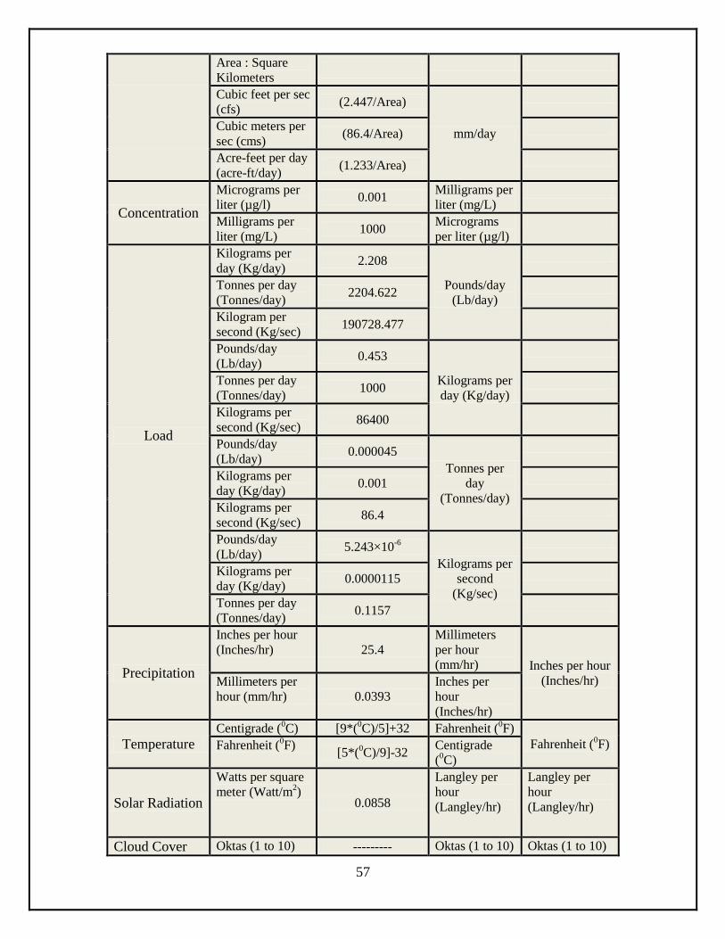
Table 2: Variable unit conversion options and conversion values used in HDFT........................ 56

viii

Foreword

Water availability and water quality models are widely used for environmental regulation such as

developing Total Maximum Daily Loads (TMDLs) for water quality-impaired water bodies,

environmental policy (e.g., water quality criteria development), and sustainable development and

management of land and water resources. To meet EPA’s goals, the National Exposure Research

Laboratory (NERL) develops and uses fate and transport models, modeling tools and approaches

to simulate water availability and water quality constituents. The Hydrological Simulation

Program - FORTRAN (HSPF) is a comprehensive watershed model capable of simulating water

availability and water quality constituents at user-specified spatial and temporal scales. HSPF is

a mixed land-use model applicable to both urban and non-urban watersheds and was developed

by EPA in collaboration with the United States Geological Survey (USGS). HSPF is the core

watershed model in the BASINS (Better Assessment Science Integrating Point and Nonpoint

Source Pollution) modeling system. While BASINS has a number of databases available to

HSPF users, oftentimes model users need to create HSPF simulations with data from sources

other than BASINS. Because HSPF requires extensive input data, the HSPF Data-Formatting

Tool (HDFT) allows users to format model input data and import it into a WDM file. This tool is

also for users who are building their data from scratch from study areas outside of the United

States. HDFT aids HSPF’s GRAY and GREEN infrastructure modeling applications that use

sub-hourly temporal resolutions. GRAY infrastructure is most often used in urban environments

where stormwater usually flows into stormwater system pipes before reaching a local stream,

lake, or wastewater treatment plant. GREEN infrastructure systems mimic natural processes to

infiltrate, evaporate, and/or reuse stormwater to maintain the pre-development hydrology and

water quality of urban environments.

ix

Acknowledgements

I would like to thank Jimmy Bisese for assistance with the Storage Retrieval Data Warehouse

(STORET) web services and David Valentine for assistance with the Consortium of Universities

for the Advancement of Hydrologic Science, Inc. (CUAHSI) web services. I would also like to

thank Fran Rauschenberg for reviewing the report.

1

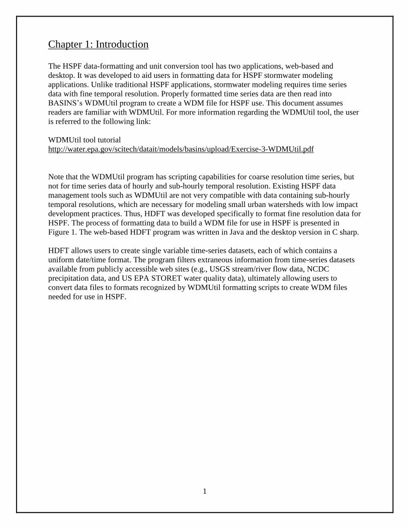
Chapter 1: Introduction

The HSPF data-formatting and unit conversion tool has two applications, web-based and

desktop. It was developed to aid users in formatting data for HSPF stormwater modeling

applications. Unlike traditional HSPF applications, stormwater modeling requires time series

data with fine temporal resolution. Properly formatted time series data are then read into

BASINS’s WDMUtil program to create a WDM file for HSPF use. This document assumes

readers are familiar with WDMUtil. For more information regarding the WDMUtil tool, the user

is referred to the following link:

WDMUtil tool tutorial

http://water.epa.gov/scitech/datait/models/basins/upload/Exercise-3-WDMUtil.pdf

Note that the WDMUtil program has scripting capabilities for coarse resolution time series, but

not for time series data of hourly and sub-hourly temporal resolution. Existing HSPF data

management tools such as WDMUtil are not very compatible with data containing sub-hourly

temporal resolutions, which are necessary for modeling small urban watersheds with low impact

development practices. Thus, HDFT was developed specifically to format fine resolution data for

HSPF. The process of formatting data to build a WDM file for use in HSPF is presented in

Figure 1. The web-based HDFT program was written in Java and the desktop version in C sharp.

HDFT allows users to create single variable time-series datasets, each of which contains a

uniform date/time format. The program filters extraneous information from time-series datasets

available from publicly accessible web sites (e.g., USGS stream/river flow data, NCDC

precipitation data, and US EPA STORET water quality data), ultimately allowing users to

convert data files to formats recognized by WDMUtil formatting scripts to create WDM files

needed for use in HSPF.


2

Figure 1: Main Process

3

HDFT (Web–Version)

4

Chapter 2: Data-Pasting Option of the HDFT Web-Version

HDFT has been tested with several data formats, including streamflow, meteorological, and

water quality data obtained from the United States Geological Survey (USGS) and the National

Climate Data Center (NCDC). It can download EPA STORET, USGS NWIS, and Instantaneous

Data using CUAHSI and STORET web services. Our intention is to simplify preparing input

data to use within the HSPF model. Although many data types and formats are included in this

Report, other formats currently may be unsupported. Users are encouraged to contact HDFT

developers about unsupported data formats to facilitate their inclusion in future versions of the

program.

Although the primary function of HDFT is to format input datasets properly, convert variable

units, and export the resulting formatted data directly to a file (desktop version) or by copying

and pasting the formatted data into a document (web version), it only incorporates one variable

(e.g., precipitation) at a time. For both desktop and web versions, users must import resulting

formatted data to a WDM file for HSPF use. Time series data that include meteorological and

streamflow data is used by HSPF. Depending on a project’s objectives, model users may need to

import data for one variable or for several. For example, in hydrological modeling applications,

only a few metrological parameters and streamflow data are needed. In water quality modeling

applications, however, HSPF model users need additional meteorological data such as cloud

cover, solar radiation, wind speed, and dew point temperature. While HDFT can format data for

all HSPF applications, it was specifically developed for stormwater modeling as this application

requires fine temporal resolution rainfall data ranging from one minute to one hour.

HDFT formats time series data and can convert variable units to those useable by HSPF, as

shown in Table 1, located in Appendix-A. Note that various model input data can come from

several sources such as the USGS, NCDC (ASOS 1 min data, etc.). HDFT minimizes the time

required to format, convert, and export time series data for the HSPF model. Although HDFT

can make many user-specified conversions, it only lists conversions for 10 common variables.

WDM formatting scripts provided in BASINS are not able to format hourly and sub-hourly time

series data properly, as such, additional scripts are included with the tool that allow users to

incorporate data of fine temporal resolution into WDM files.

The web-version of HDFT has two data import options: pasting data to the tool (user data) and

downloading data from the web. Pasting directly to the tool allows HDFT users to format their

locally stored data properly and the download option allows users to get data directly from

USGS or EPA STORET websites.

5

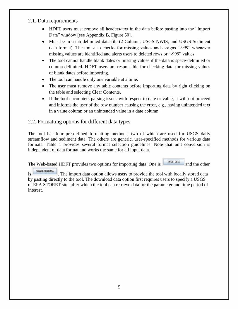
2.1. Data requirements

HDFT users must remove all headers/text in the data before pasting into the “Import

Data” window [see Appendix B, Figure 50].

Must be in a tab-delimited data file (2 Column, USGS NWIS, and USGS Sediment

data format). The tool also checks for missing values and assigns “-999” whenever

missing values are identified and alerts users to deleted rows or “-999” values. The tool cannot handle blank dates or missing values if the data is space-delimited or

comma-delimited. HDFT users are responsible for checking data for missing values

or blank dates before importing. The tool can handle only one variable at a time.

The user must remove any table contents before importing data by right clicking on

the table and selecting Clear Contents.

If the tool encounters parsing issues with respect to date or value, it will not proceed

and informs the user of the row number causing the error, e.g., having unintended text

in a value column or an unintended value in a date column.

2.2. Formatting options for different data types

The tool has four pre-defined formatting methods, two of which are used for USGS daily

streamflow and sediment data. The others are generic, user-specified methods for various data

formats. Table 1 provides several format selection guidelines. Note that unit conversion is

independent of data format and works the same for all input data.

The Web-based HDFT provides two options for importing data. One is and the other

is . The import data option allows users to provide the tool with locally stored data

by pasting directly to the tool. The download data option first requires users to specify a USGS

or EPA STORET site, after which the tool can retrieve data for the parameter and time period of

interest.

6

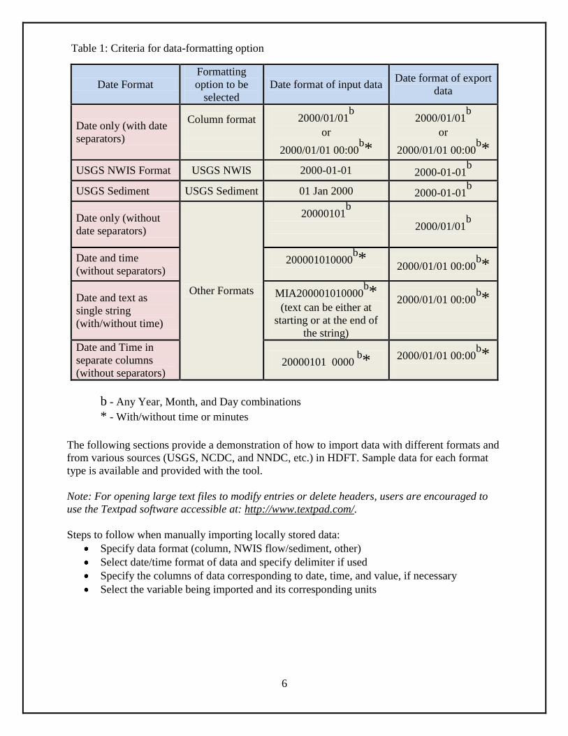
Table 1: Criteria for data-formatting option

Date Format

Formatting

option to be

selected

Date format of input data Date format of export

data

Date only (with date

separators)

Column format

2000/01/01b

or

2000/01/01 00:00b*

2000/01/01b

or

2000/01/01 00:00b*

USGS NWIS Format USGS NWIS 2000-01-01 2000-01-01b

USGS Sediment USGS Sediment 01 Jan 2000 2000-01-01b

Date only (without

date separators)

Other Formats

20000101b

2000/01/01b

Date and time

(without separators) 200001010000

b*

2000/01/01 00:00

b*

Date and text as

single string

(with/without time)

MIA200001010000b*

(text can be either at

starting or at the end of

the string)

2000/01/01 00:00b*

Date and Time in

separate columns

(without separators) 20000101 0000

b* 2000/01/01 00:00

b*

b - Any Year, Month, and Day combinations

* - With/without time or minutes

The following sections provide a demonstration of how to import data with different formats and

from various sources (USGS, NCDC, and NNDC, etc.) in HDFT. Sample data for each format

type is available and provided with the tool.

Note: For opening large text files to modify entries or delete headers, users are encouraged to

use the Textpad software accessible at: http://www.textpad.com/.

Steps to follow when manually importing locally stored data:

Specify data format (column, NWIS flow/sediment, other)

Select date/time format of data and specify delimiter if used

Specify the columns of data corresponding to date, time, and value, if necessary

Select the variable being imported and its corresponding units

http://www.textpad.com/

7

2.3. Column Format (user-specified formatting option)

The column format works with any of these date formats -- YYYY/MM/DD, MM/DD/YYYY,

and DD/MM/YYYY, with or without time. Appendix B [Figure 51] illustrates sample data with

column format. Steps to follow when importing data with column format are given in the

following section.

Note: After removing headers within data text files, it is advisable to import data to a

spreadsheet. An application like Microsoft Excel allows users to copy and paste column-

formatted data into the HDFT tool easily.

2.3.1. Formatting Column Format Data

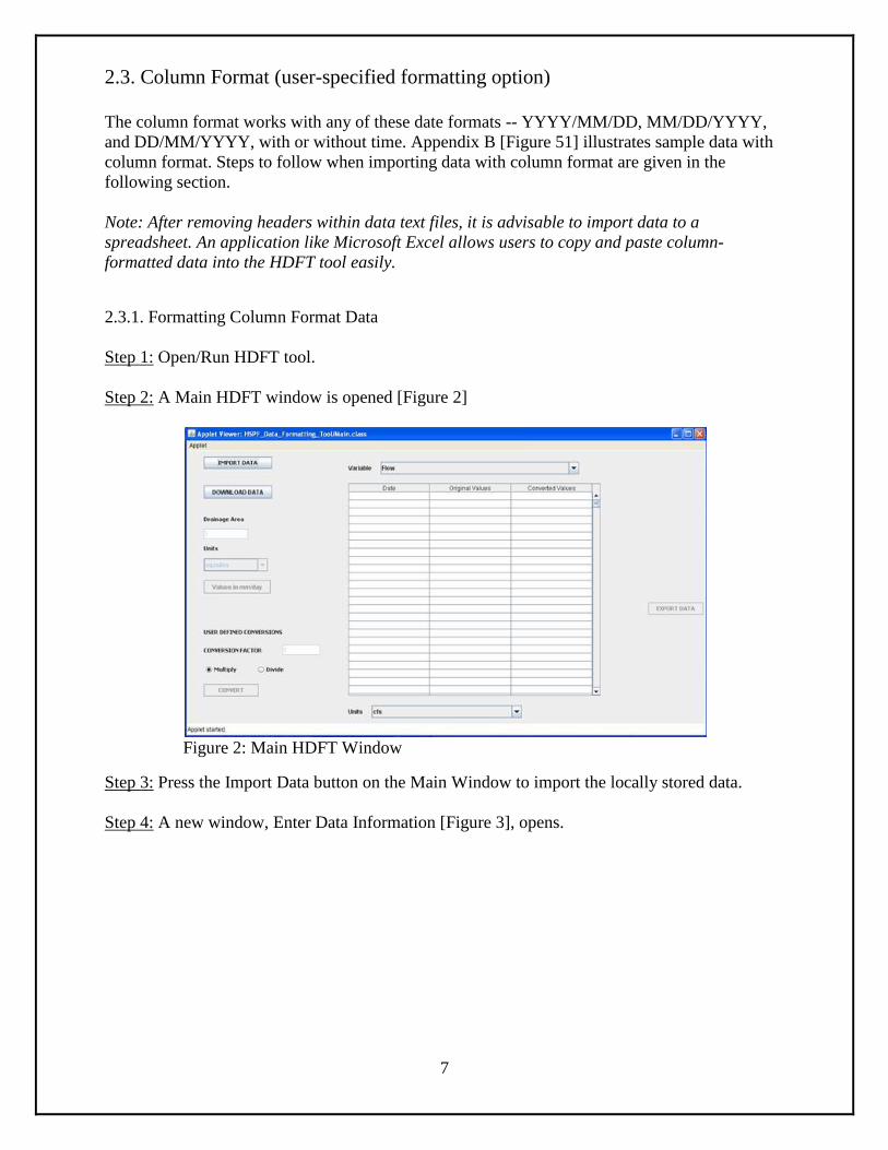
Step 1: Open/Run HDFT tool.

Step 2: A Main HDFT window is opened [Figure 2]

Figure 2: Main HDFT Window

Step 3: Press the Import Data button on the Main Window to import the locally stored data.

Step 4: A new window, Enter Data Information [Figure 3], opens.

8

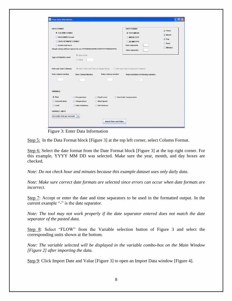
Figure 3: Enter Data Information

Step 5: In the Data Format block [Figure 3] at the top left corner, select Column Format.

Step 6: Select the date format from the Date Format block [Figure 3] at the top right corner. For

this example, YYYY MM DD was selected. Make sure the year, month, and day boxes are

checked.

Note: Do not check hour and minutes because this example dataset uses only daily data.

Note: Make sure correct date formats are selected since errors can occur when date formats are

incorrect.

Step 7: Accept or enter the date and time separators to be used in the formatted output. In the

current example “-” is the date separator.

Note: The tool may not work properly if the date separator entered does not match the date

separator of the pasted data.

Step 8: Select “FLOW” from the Variable selection button of Figure 3 and select the

corresponding units shown at the bottom.

Note: The variable selected will be displayed in the variable combo-box on the Main Window

[Figure 2] after importing the data.

Step 9: Click Import Date and Value [Figure 3] to open an Import Data window [Figure 4].

9

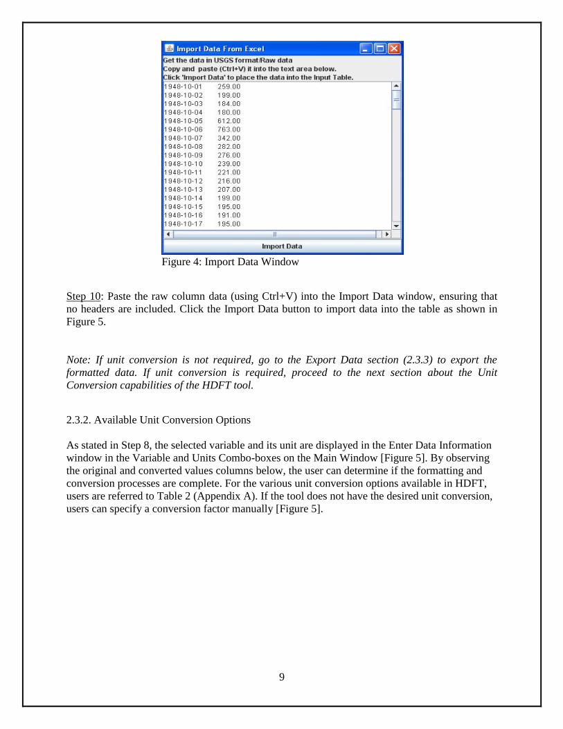
Figure 4: Import Data Window

Step 10: Paste the raw column data (using Ctrl+V) into the Import Data window, ensuring that

no headers are included. Click the Import Data button to import data into the table as shown in

Figure 5.

Note: If unit conversion is not required, go to the Export Data section (2.3.3) to export the

formatted data. If unit conversion is required, proceed to the next section about the Unit

Conversion capabilities of the HDFT tool.

2.3.2. Available Unit Conversion Options

As stated in Step 8, the selected variable and its unit are displayed in the Enter Data Information

window in the Variable and Units Combo-boxes on the Main Window [Figure 5]. By observing

the original and converted values columns below, the user can determine if the formatting and

conversion processes are complete. For the various unit conversion options available in HDFT,

users are referred to Table 2 (Appendix A). If the tool does not have the desired unit conversion,

users can specify a conversion factor manually [Figure 5].

10

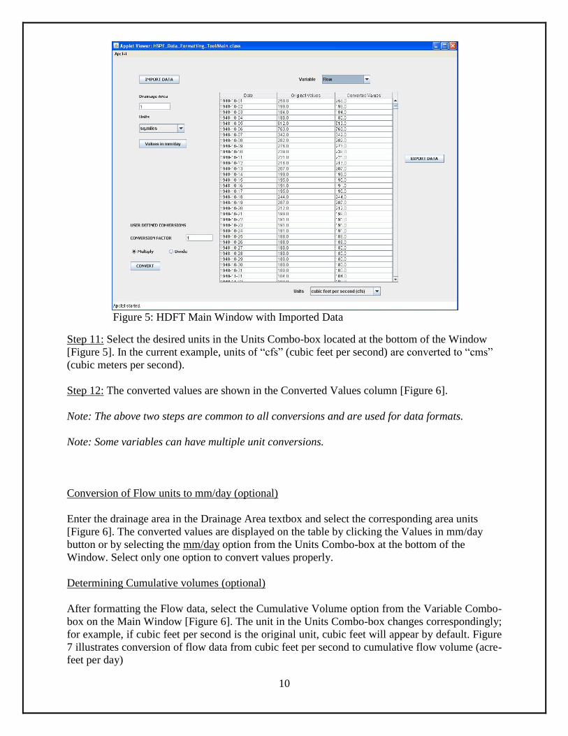
Figure 5: HDFT Main Window with Imported Data

Step 11: Select the desired units in the Units Combo-box located at the bottom of the Window

[Figure 5]. In the current example, units of “cfs” (cubic feet per second) are converted to “cms”

(cubic meters per second).

Step 12: The converted values are shown in the Converted Values column [Figure 6].

Note: The above two steps are common to all conversions and are used for data formats.

Note: Some variables can have multiple unit conversions.

Conversion of Flow units to mm/day (optional)

Enter the drainage area in the Drainage Area textbox and select the corresponding area units

[Figure 6]. The converted values are displayed on the table by clicking the Values in mm/day

button or by selecting the mm/day option from the Units Combo-box at the bottom of the

Window. Select only one option to convert values properly.

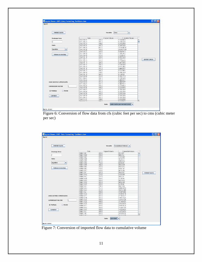
Determining Cumulative volumes (optional)

After formatting the Flow data, select the Cumulative Volume option from the Variable Combo-

box on the Main Window [Figure 6]. The unit in the Units Combo-box changes correspondingly;

for example, if cubic feet per second is the original unit, cubic feet will appear by default. Figure

7 illustrates conversion of flow data from cubic feet per second to cumulative flow volume (acre-

feet per day)

11

Figure 6: Conversion of flow data from cfs (cubic feet per sec) to cms (cubic meter

per sec)

Figure 7: Conversion of imported flow data to cumulative volume

12

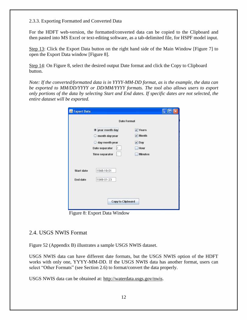
2.3.3. Exporting Formatted and Converted Data

For the HDFT web-version, the formatted/converted data can be copied to the Clipboard and

then pasted into MS Excel or text-editing software, as a tab-delimited file, for HSPF model input.

Step 13: Click the Export Data button on the right hand side of the Main Window [Figure 7] to

open the Export Data window [Figure 8].

Step 14: On Figure 8, select the desired output Date format and click the Copy to Clipboard

button.

Note: If the converted/formatted data is in YYYY-MM-DD format, as is the example, the data can

be exported to MM/DD/YYYY or DD/MM/YYYY formats. The tool also allows users to export

only portions of the data by selecting Start and End dates. If specific dates are not selected, the

entire dataset will be exported.

Figure 8: Export Data Window

2.4. USGS NWIS Format

Figure 52 (Appendix B) illustrates a sample USGS NWIS dataset.

USGS NWIS data can have different date formats, but the USGS NWIS option of the HDFT

works with only one, YYYY-MM-DD. If the USGS NWIS data has another format, users can

select “Other Formats” (see Section 2.6) to format/convert the data properly.

USGS NWIS data can be obtained at: http://waterdata.usgs.gov/nwis.

http://waterdata.usgs.gov/nwis

13

2.4.1. Formatting NWIS Data

Repeat Steps 1 through 4 of Section 2.3.1.

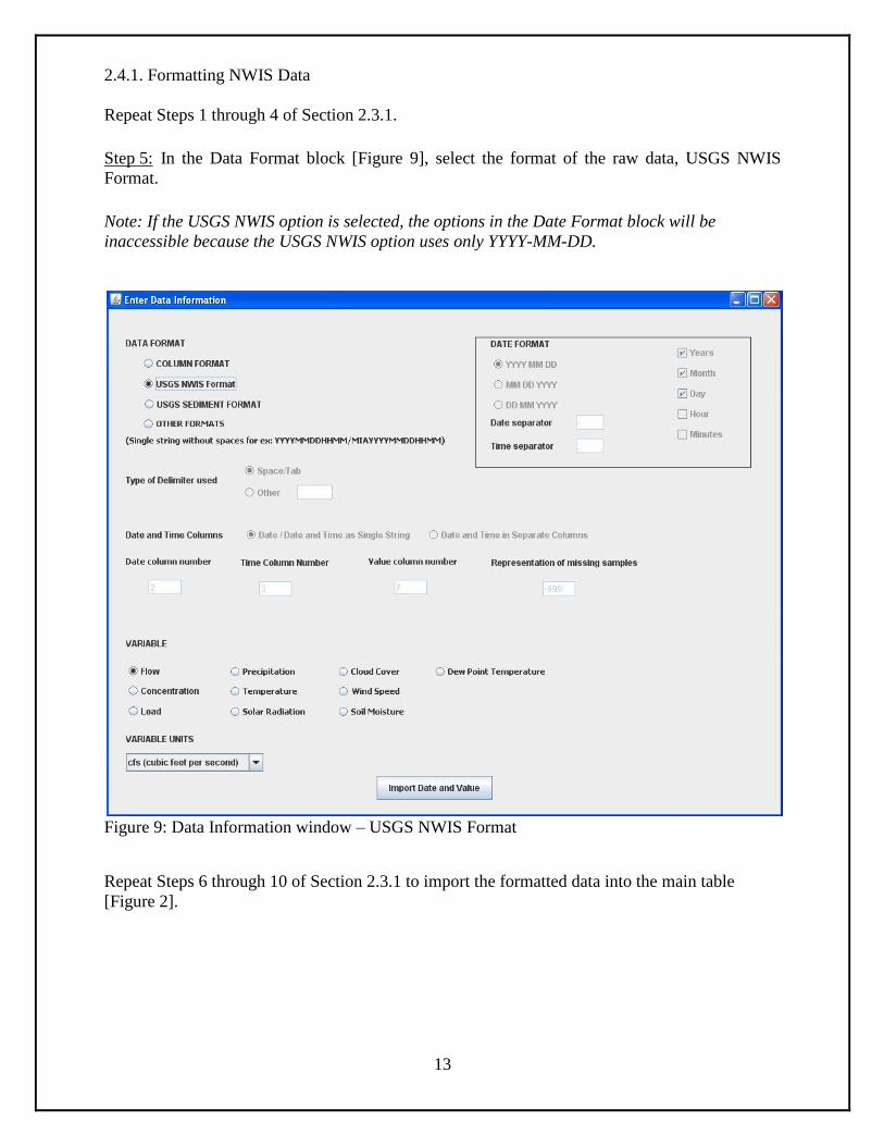
Step 5: In the Data Format block [Figure 9], select the format of the raw data, USGS NWIS

Format.

Note: If the USGS NWIS option is selected, the options in the Date Format block will be

inaccessible because the USGS NWIS option uses only YYYY-MM-DD.

Figure 9: Data Information window – USGS NWIS Format

Repeat Steps 6 through 10 of Section 2.3.1 to import the formatted data into the main table

[Figure 2].

14


Repeat Section 2.3.2. to convert the imported data to different units.


Repeat Section 2.3.3. to export the formatted/converted data.

2.5. USGS Sediment format

Figure 53 (Appendix B) illustrates sample USGS Sediment data.

The USGS Sediment data has a DD-MMM-YYYY date format and HDFT converts this to

YYYY-MM-DD format before importing data into the table.

The USGS Sediment data can be obtained at: http://co.water.usgs.gov/sediment/

2.5.1. Formatting USGS Sediment Data


Step 5: In the Data Format block [Figure 9], select the raw data’s format, USGS Sediment

format.

Note: If the USGS Sediment option is selected, options in the Date Format block will be

inaccessible since the USGS Sediment option uses only DD-MMM-YYYY

Repeat Steps 6 through 10 of Section 2.3.1. to import formatted data into the Main Page table

[Figure 2].





http://co.water.usgs.gov/sediment/

15

2.6. Other Formats

This option works with multiple data formats to format data collected by different federal

agencies for use within HSPF.

Data requirement

The date format should be a single string (without spaces), with date and time in the same

or separate columns

The date/time sample may have text such as MIA2009051819000000 at the beginning or

end of the string

Date or value should not be blank, especially when data is space-delimited

2.6.1. NOAA ASOS (1 Minute Data)

Figure 54 (Appendix-B) illustrates sample ASOS data (1 Minute Data).

ASOS data can be obtained from:

http://www.ncdc.noaa.gov/oa/climate/climatedata.html#asosminutedata

2.6.1.1. Importing ASOS data

Note: Clear any existing data by right clicking on the table and selecting Clear Contents.

Repeat Steps 1 through 4 of Section 2.3.1

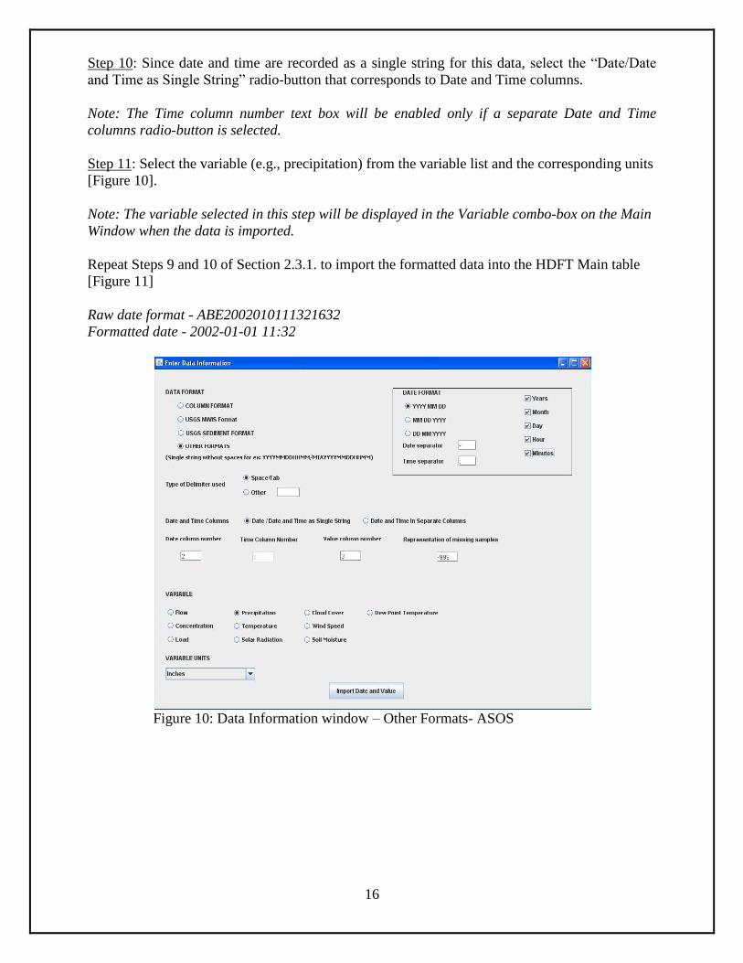
Step 5: In the Data Format block [Figure 10], select Other Formats and then Date column and

Value column by typing numbers in their respective textboxes [Figure 10].

For the example ASOS data, the Date column number is 2 and the Value column number is 3

[Figure 10].

Step 6: Select the format from the Date Format block [Figure 10] that corresponds to the Data

format (e.g., YYYY MM DD in this example) and check the hour and minute checkboxes since

this data has date and time formats.

Step 7: Accept or enter the date and time separators that correspond to the data. In the current

example, “-” is used as the date separator.

Note: Specifying the correct date format and temporal resolution is necessary for HDFT to read

the input data properly. Date and time separators are specified, to control the characters used

by the tool to separate date/time in the formatted data.

Step 8: Select/Enter a delimiter for the dataset. In the current example, Space/Tab delimiter is

selected.

Step 9: Enter the missing samples identifier to identify them or leave the default value as “-999.”

http://www.ncdc.noaa.gov/oa/climate/climatedata.html#asosminutedata

16

Step 10: Since date and time are recorded as a single string for this data, select the “Date/Date

and Time as Single String” radio-button that corresponds to Date and Time columns.

Note: The Time column number text box will be enabled only if a separate Date and Time

columns radio-button is selected.

Step 11: Select the variable (e.g., precipitation) from the variable list and the corresponding units

[Figure 10].

Note: The variable selected in this step will be displayed in the Variable combo-box on the Main

Window when the data is imported.

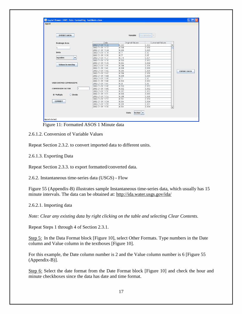
Repeat Steps 9 and 10 of Section 2.3.1. to import the formatted data into the HDFT Main table

[Figure 11]

Raw date format - ABE2002010111321632

Formatted date - 2002-01-01 11:32

Figure 10: Data Information window – Other Formats- ASOS

17

Figure 11: Formatted ASOS 1 Minute data

2.6.1.2. Conversion of Variable Values

Repeat Section 2.3.2. to convert imported data to different units.

2.6.1.3. Exporting Data

Repeat Section 2.3.3. to export formatted/converted data.

2.6.2. Instantaneous time-series data (USGS) - Flow

Figure 55 (Appendix-B) illustrates sample Instantaneous time-series data, which usually has 15

minute intervals. The data can be obtained at: http://ida.water.usgs.gov/ida/

2.6.2.1. Importing data



Step 5: In the Data Format block [Figure 10], select Other Formats. Type numbers in the Date

column and Value column in the textboxes [Figure 10].

For this example, the Date column number is 2 and the Value column number is 6 [Figure 55

(Appendix-B)].

Step 6: Select the date format from the Date Format block [Figure 10] and check the hour and

minute checkboxes since the data has date and time format.

http://ida.water.usgs.gov/ida/

18

Step 7: Accept or enter the date and time separators corresponding to the data. In the current


Step 8: Select/Enter the delimiter used for the dataset. In the current example, Space/Tab

delimiter is selected.

Step 9: Enter the missing samples identifier to indicate the presence of missing data or leave the

default value as “-999”.

Step 10: Since date and time are in a single string for the example data, we used the default Date

and Time columns selection “Date/Date and Time as Single String.”

Note: The Date and Time column number textboxes are enabled only when the Date and Time in

Separate Columns radio-button is selected.

Step 11: Select the variable (e.g., flow) from the variable list and its corresponding units (e.g.,

cfs).

Note: The variable selected in this step will be displayed in the Variable combo-box on the Main

window when the data is imported.

Repeat Steps 9 and 10 of Section 2.3.1. to import the formatted data into the Main Page table

[see Figure 11]

Raw Date Format - 20040127000000

Formatted date - 2004-01-27 00:00


Repeat Section 2.3.2 to convert the imported data to different units.


Repeat Section 2.3.3 to export the formatted/converted data.

2.6.3. Hourly data NCDC - U.S. Climate Reference Network (USCRN) – Temperature

Figure 56 (Appendix-B) illustrates sample NNDC hourly climate data obtained from:

http://gis.ncdc.noaa.gov/map/cdo/

2.6.3.1 Importing data



Step 5: In the Data Format block [Figure 10], select Other Formats and specify the Date column

number and Value column number. The data in this example has a Date column number of “1”

and Value column number of “14” [Figure 56 (Appendix B)].


19

Step 6: Select the date format from the Date Format block [Figure 10] and check the hour

checkbox, but not the minute checkbox since this is hourly data.

Step 7: Accept or enter the date and time separators corresponding to the data. In the current


Step 8: Enter the missing samples identifier to identify missing samples. In the current example,

-999 is used.

Step 9: Since the data for this example is comma-delimited, select Other under the Type of

Delimiter Used and enter a comma (“,”) into the delimiter textbox to specify the delimiter used

for the dataset [Figure 10].

Step 10: Select the variable (e.g., temperature) from the variable list and the corresponding unit

(e.g., Centigrade).

Repeat Steps 9 and 10 of Section 2.3.1. to import the formatted data into the HDFT Main table

[Figure 12].





20

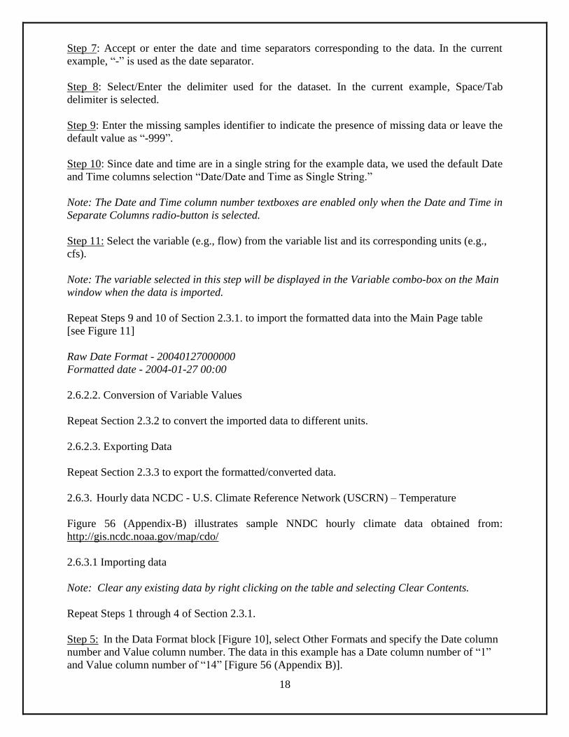
Figure 12: Formatted NCDC hourly climate data

2.6.4. NCDC- DS3505 - Surface Data, Hourly Global – Date and Time in Separate Columns –

Solar Radiation

Figure 58 (Appendix B) illustrates sample NCDC hourly global climate data. Global climate data

can be obtained from: http://gis.ncdc.noaa.gov/map/cdo/

2.6.4.1. Importing data



Step 5: In the Data Format block [Figure 10], select Other Formats and the Date column and

Value column numbers in their respective textboxes.

Step 6: Select the correct date format from the Date Format block [Figure 10] and check the hour

and minute checkboxes since the data have both date and time formats.

Step 7: Accept or enter the date and time separator that corresponds to the raw data. In the

current example, “-” is used as the date separator.

Step 8: Select/Enter the raw data delimiter. In the current example, Space/Tab option is selected.


21

Step 9: Select Date and Time in the separate columns radio button, the Time Column Number

textbox will now be accessible.

Step 10: Enter the column number associated with the time string.

In the current example, enter value “3” in the Date column number textbox, “4” in the Time

column number textbox, and “7” in Value column number textbox.

Step 11: Enter the missing samples identifier to identify missing samples or leave the default

value, “-999.”

Step 12: Select the variable from the variable list (e.g., Solar Radiation) and the corresponding

units (e.g., Langley per Hr).

Note: The selected variable will be displayed in the Variable combo-box on the Main window

after importing the data.

Repeat Steps 9 and 10 of Section 2.3.1. to import the formatted data into the table on the Main

Page (similar to Figure 12).

Raw Date Format – 20040127 0000

Formatted date - 2004-01-27 00:00





22

Chapter 3: HDFT Data Downloading Options (Web-version)

In addition to handling different data formats imported into the HDFT web-version with data-

pasting, as discussed in the previous chapter, web-version users have data download options to

retrieve flow and water quality data directly from the following sources:

USGS NWIS Data (Daily data)

USGS Instantaneous Irregular data

EPA-STORET

Compared to data-pasting, downloading is faster and more efficient. It is limited, however, by

the availability of web services and databases amenable to web download. The download option

uses web services provided by the Consortium of Universities for the Advancement of

Hydrological Science (CUAHSI) and EPA-STORET. A web service is a way for devices to

communicate over the web using standard protocols -- specifically, they automate transfer of

available data from one location to another. For additional information regarding data download

using CUASHI and other services, HDFT users may refer to: http://www.cuahsi.org/ or to

http://www.w3.org/TR/ws-arch/ for additional information.

Using the CUASHI web services, the HDFT tool can download about 15 parameters (physical,

nutrient, microbiological). Using the EPA-STORET, the tool can download any parameter

available in the STORET database. For practical reasons, we limited the variable groups

downloaded from one station to four types -- physical, nutrient, microbiological, and other.

When the data of interest have multiple measurements taken on a single day, HDFT imports only

the average value of the parameter; it also sorts the data by date. Multiple measurements in a

single day are common to USGS Instantaneous data, but less so to EPA-STORET databases.

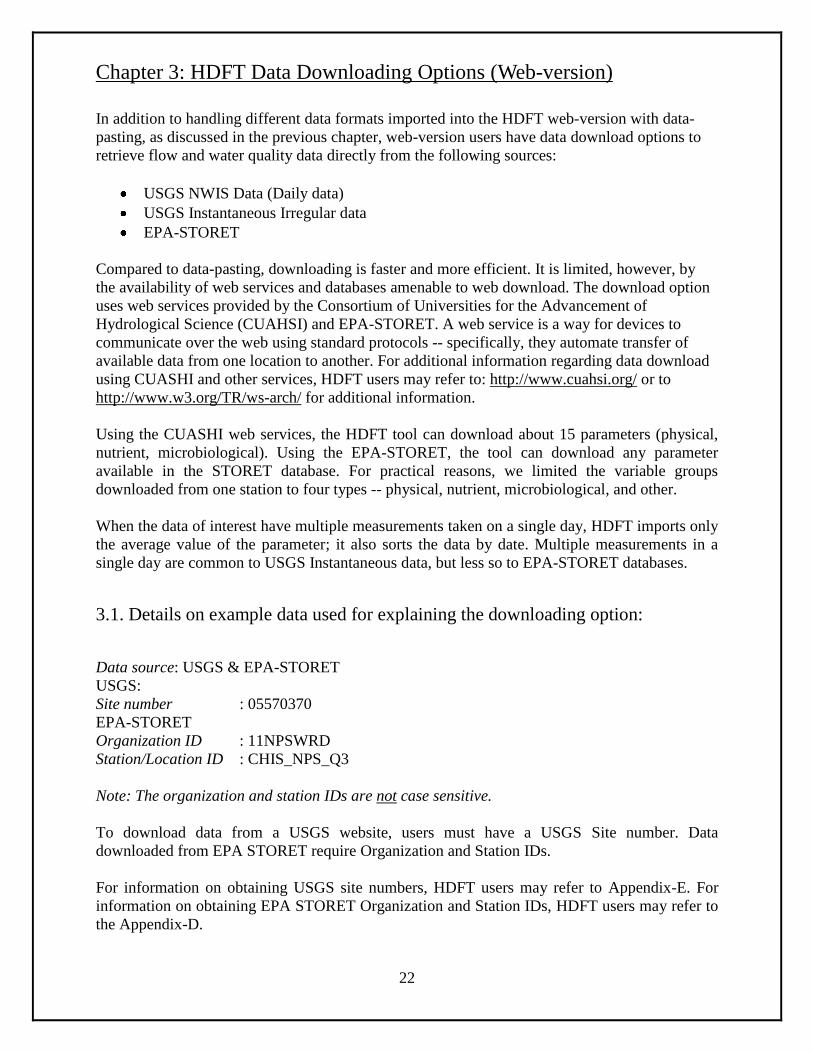
3.1. Details on example data used for explaining the downloading option:

Data source: USGS & EPA-STORET

USGS:

Site number : 05570370

EPA-STORET

Organization ID : 11NPSWRD

Station/Location ID : CHIS_NPS_Q3

Note: The organization and station IDs are not case sensitive.

To download data from a USGS website, users must have a USGS Site number. Data

downloaded from EPA STORET require Organization and Station IDs.

For information on obtaining USGS site numbers, HDFT users may refer to Appendix-E. For

information on obtaining EPA STORET Organization and Station IDs, HDFT users may refer to

the Appendix-D.

http://www.cuahsi.org/

http://www.w3.org/TR/ws-arch/

23

3.2. Steps to follow when downloading the data are:

Enter Station ID (USGS) or Organization and Station IDs (EPA-STORET)

Select a variable

Extract station and parameter information – Station name, Parameter units (if available)

and Start and End dates

Enter dates for which data is required

Download Data

3.3. Downloading data from USGS NWIS Daily data & USGS Instantaneous

Irregular Data

Clear any existing data by right clicking on the table and selecting Clear Contents.

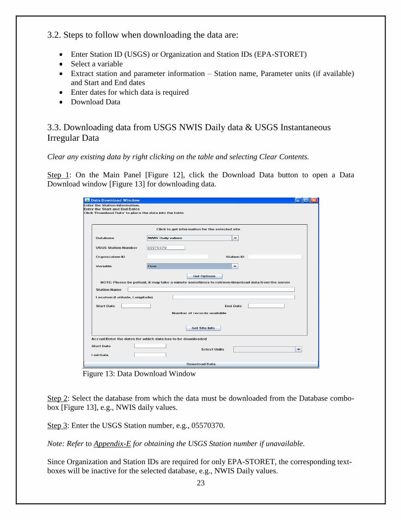
Step 1: On the Main Panel [Figure 12], click the Download Data button to open a Data

Download window [Figure 13] for downloading data.

Figure 13: Data Download Window

Step 2: Select the database from which the data must be downloaded from the Database combo-

box [Figure 13], e.g., NWIS daily values.

Step 3: Enter the USGS Station number, e.g., 05570370.

Note: Refer to Appendix-E for obtaining the USGS Station number if unavailable.

Since Organization and Station IDs are required for only EPA-STORET, the corresponding text-

boxes will be inactive for the selected database, e.g., NWIS Daily values.

24

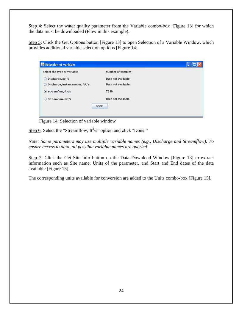
Step 4: Select the water quality parameter from the Variable combo-box [Figure 13] for which

the data must be downloaded (Flow in this example).

Step 5: Click the Get Options button [Figure 13] to open Selection of a Variable Window, which

provides additional variable selection options [Figure 14].

Figure 14: Selection of variable window

Step 6: Select the “Streamflow, ft3/s” option and click "Done.”

Note: Some parameters may use multiple variable names (e.g., Discharge and Streamflow). To

ensure access to data, all possible variable names are queried.

Step 7: Click the Get Site Info button on the Data Download Window [Figure 13] to extract

information such as Site name, Units of the parameter, and Start and End dates of the data

available [Figure 15].

The corresponding units available for conversion are added to the Units combo-box [Figure 15].

25

Figure 15: Data Download Window with Station information extracted

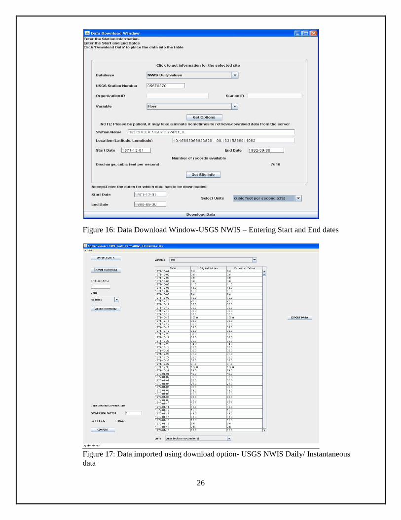
Step 8: Enter required Start and End dates based on the above available information, and select

the units for the available parameter in the Select Units combo-box, e.g., cubic feet per second

(cfs) [Figure 16].

Important: When entering Start and End dates, use the same date format (including date

separators) as displayed in Begin and Last Date textboxes. In the current example, the date

format is YYYY-MM-DD.

Step 9: After clicking the Download Data button [Figure 16], the data (date and value) will be

downloaded to the table on the Main Panel [Figure 17].

The steps for downloading data from the USGS Instantaneous irregular data are similar to

downloading USGS Daily Data. Start by selecting USGS Instantaneous irregular data from the

database combo-box in Step 2.

Repeat Section 2.3.2. to convert the imported data to different units and repeat Section 2.3.3. to

export the raw or converted data.

26

Figure 16: Data Download Window-USGS NWIS – Entering Start and End dates

Figure 17: Data imported using download option- USGS NWIS Daily/ Instantaneous

data

27

3.4. Downloading Data from EPA-STORET

Downloading data from EPA STORET is slightly different from USGS NWIS. Data from the

USGS NWIS is downloaded using Station number only and a unique identifier for each

parameter; EPA-STORET uses organization ID, station ID, and a parameter name. EPA-

STORET parameter names and IDs are not unique, and data uploaded from different states and

organizations may have different parameter names for the same water quality constituent. For

example, some sites use “Total suspended solids” while others use “Solids, suspended.” Thus,

using different names for the same parameter may give erroneous results or provide less data

than is actually available in the database. To avoid errors caused by non-unique parameter

names, an intermediate step to show all data available at a STORET site was implemented,

allowing HDFT users to view a list of variables for download which facilitates parameter

selection.

The above issues and, potentially, others may not create problems in downloading available data;

however, issues may arise in unit-conversion, requiring users to select “Other” in the Select

unit’s combo-box [Figure 16]. Selecting “Other” units allows users to define conversion options

manually by entering the factor to be used to change units of the downloaded data on the left-

hand side of the Main Panel [Figure 17].

The following steps explain how to download data from EPA-STORET.

Clear any existing data on the table by right clicking on the table and select Clear Contents.

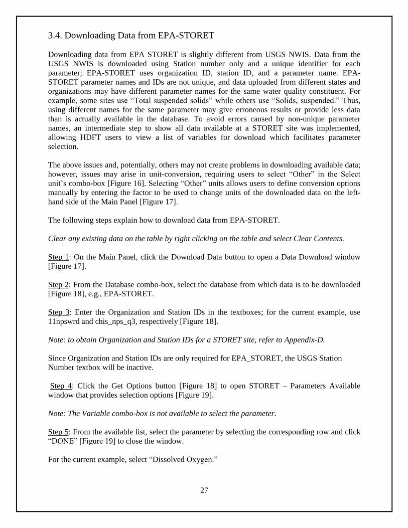
Step 1: On the Main Panel, click the Download Data button to open a Data Download window

[Figure 17].

Step 2: From the Database combo-box, select the database from which data is to be downloaded

[Figure 18], e.g., EPA-STORET.

Step 3: Enter the Organization and Station IDs in the textboxes; for the current example, use

11npswrd and chis_nps_q3, respectively [Figure 18].

Note: to obtain Organization and Station IDs for a STORET site, refer to Appendix-D.

Since Organization and Station IDs are only required for EPA_STORET, the USGS Station

Number textbox will be inactive.

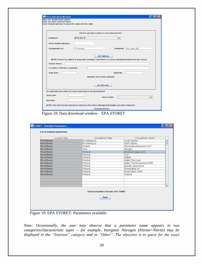
Step 4: Click the Get Options button [Figure 18] to open STORET – Parameters Available

window that provides selection options [Figure 19].

Note: The Variable combo-box is not available to select the parameter.

Step 5: From the available list, select the parameter by selecting the corresponding row and click

“DONE” [Figure 19] to close the window.

For the current example, select “Dissolved Oxygen.”

28

Figure 18: Data download window – EPA STORET

Figure 19: EPA STORET- Parameters available

Note: Occasionally, the user may observe that a parameter name appears in two

categories/characteristic types -- for example, Inorganic Nitrogen (Nitrate+Nitrite) may be

displayed in the “Nutrient” category and in “Other”. The objective is to query for the exact

29

name of the parameter, which is not constant for every site, to avoid issues while downloading

data. The tool will download all available data that corresponds to the selected parameter.

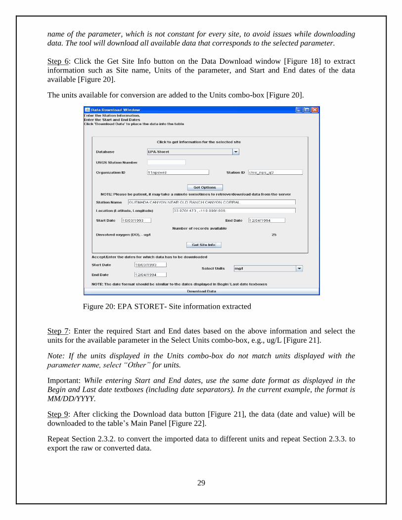
Step 6: Click the Get Site Info button on the Data Download window [Figure 18] to extract

information such as Site name, Units of the parameter, and Start and End dates of the data

available [Figure 20].

The units available for conversion are added to the Units combo-box [Figure 20].

Figure 20: EPA STORET- Site information extracted

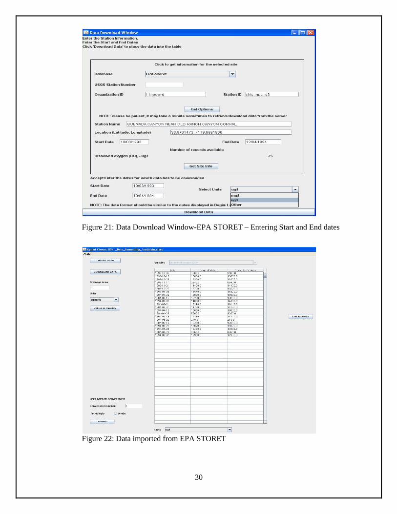
Step 7: Enter the required Start and End dates based on the above information and select the

units for the available parameter in the Select Units combo-box, e.g., ug/L [Figure 21].

Note: If the units displayed in the Units combo-box do not match units displayed with the

parameter name, select “Other” for units.

Important: While entering Start and End dates, use the same date format as displayed in the

Begin and Last date textboxes (including date separators). In the current example, the format is

MM/DD/YYYY.

Step 9: After clicking the Download data button [Figure 21], the data (date and value) will be

downloaded to the table’s Main Panel [Figure 22].

Repeat Section 2.3.2. to convert the imported data to different units and repeat Section 2.3.3. to

export the raw or converted data.

30

Figure 21: Data Download Window-EPA STORET – Entering Start and End dates

Figure 22: Data imported from EPA STORET

31

HDFT (Desktop Version 1.0)

32

Chapter 4: HDFT (Desktop Version)

4.1. Introduction

The desktop version’s formatting and data-conversion capabilities are limited since its intended

use is for large datasets the web-based version cannot handle. Further, the desktop version can

read and write data text files -- a flexibility the Java-based web-tool does not have because of

security concerns.

Preparing model input data can take considerable time and formatting errors may impact model

performance. This manual provides data formatting and conversion information for a web-based

tool and a desktop tool. Outputs from HDFT are importable to a WDM file, a FORTRAN binary

direct-access file used by hydrological and water quality models such as the Hydrological

Simulation Program –FORTRAN (HSPF). The primary purpose of HDFT is to create a text-

based time series data file that can be read by the WDMUtil tool and, in conjunction with

WDMUtil formatting scripts, populate a WDM file with time series data for the HSPF watershed

model.

The user interacts with the program to gather information necessary to process the imported data.

At most, 250 lines of data are initially read from the imported file, or all of it, if the file is

smaller. Once the user supplies required information, the entire file is processed and written one

line at a time to facilitate creation of extremely large data sets that cannot be read into memory

all at once.

Procedurally, the program:

imports a text file containing time-series data,

removes any extraneous header lines,

identifies data contained in the file by column (date or date-time, time, variable, variable

type and variable units),

converts variable units optionally, and

writes the date or date-time and variable values as a time series to a text file.

Date and Date-Time Parsing:

A line in the data section of the imported file is parsed into fields. Field delimiters are commas or

white space. Fields are slotted into a spreadsheet-like grid and the user identifies a column for

the date. Because the date cannot be in multiple columns, no facility option is offered for

processing such. If the imported file has dates broken into separate white space or comma-

delimited fields for year, month, and day, the file must be edited before processing. Hourly and

finer-grained data has a time-stamp associated with the date which may be part of the date

column or in a separate column. The date and/or date-time field can be delimited (usually by “/”

or “-” characters separating month, day and year portions of the date) or they can be a string of

digits representing YYYYMMDDhhmmss or some variation thereof.

33

Program limitations:

Rows with a missing variable value will show a dummy value of -999 in place of missing

values.

Rows with missing date or date-time values cannot be exported and will not display in

the export file.

Separator characters (e.g., tab, comma, or pipe) in place of a missing or blank value may

cause inaccurate data to be displayed or exported.

First rows of non-header data must contain a valid date or date-time value.

HDFT works with data that has date/date and time and single/multiple value columns, one

variable at a time. It has limited conversion and formatting capabilities since its intended use is

formatting large datasets for HSPF. This tutorial presents instructions for using HDFT with an

example instantaneous streamflow dataset from the USGS.

Unlike the web-version, the desktop version cannot download data. Nevertheless, it has a

capability the web-based version does not: it can read data directly from text files and write the

resulting formatted data to text files.

4.2 . Data File Requirements

The program reads all data from a data file, displaying only 250 lines. It is able to parse many

date and time formats, a list of the data formats the tool can and cannot process are below.

Data files should be in text format.

Meta-data or header information should be less than 250 lines.

Data section of the file must be comma- or white space-delimited.

Dates must be a single string (e.g., MMDDYYYY, not “MM DD YYYY”).

The first row cannot have missing dates/values.

Imported files cannot have footers or trailing empty lines after the data section at the end

of the file.

Examples of date and date-time formats the tool can process include:

YYMMDD

MMDDYYYY

MM-DD-YY

DD/MM/YY

MMDDYYhhmm

MMDDYYYY hhmm

Jan-21-1999

Date and time in separate columns

Examples of dates and date-time formats the tool cannot process include:

YY MM DD

Jan 21 1999 23:15

YYYY.MM.DD

34

Details of the data used to explain how the tool works:

Data used as examples for this tutorial were obtained from the Sopers Branch Station (USGS

01643395) near Hyattstown, Maryland.

The data has 619767 lines of record, is 23.9 MB in size, and spans from 2004/10/27 12:50 to

2009/09/30 23:55 at 5min intervals.

Raw data format: 20040127000000

Formats to: MM/DD/YYYY hh:mm

Figure 55 (Appendix B) illustrates the sample instantaneous data.

Note: After installation, HDFT users can follow the steps below to format and convert data for

input to the HSPF model.

Note: When opening large text files to modify entries or delete headers, users are encouraged to

use the Textpad software accessible at: http://www.textpad.com/.

4.3 . Importing Data

Step 1: Download and install the program on your computer.

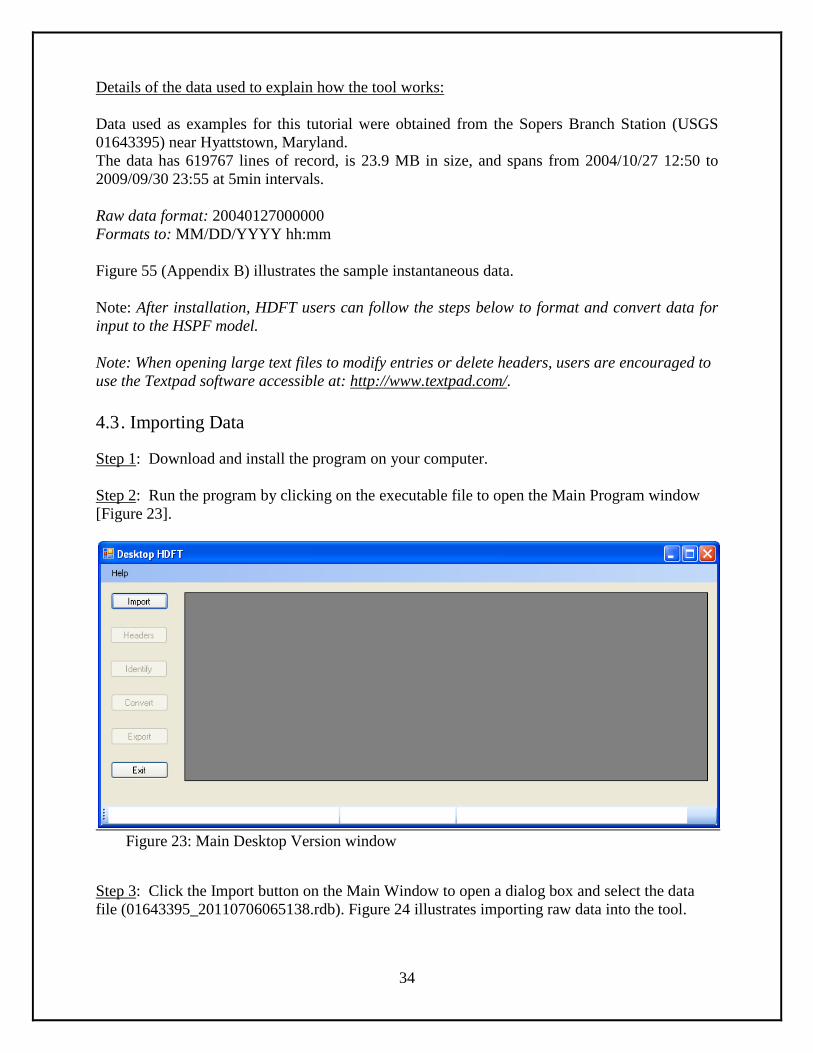
Step 2: Run the program by clicking on the executable file to open the Main Program window

[Figure 23].

Figure 23: Main Desktop Version window

Step 3: Click the Import button on the Main Window to open a dialog box and select the data

file (01643395_20110706065138.rdb). Figure 24 illustrates importing raw data into the tool.

http://www.textpad.com/

35

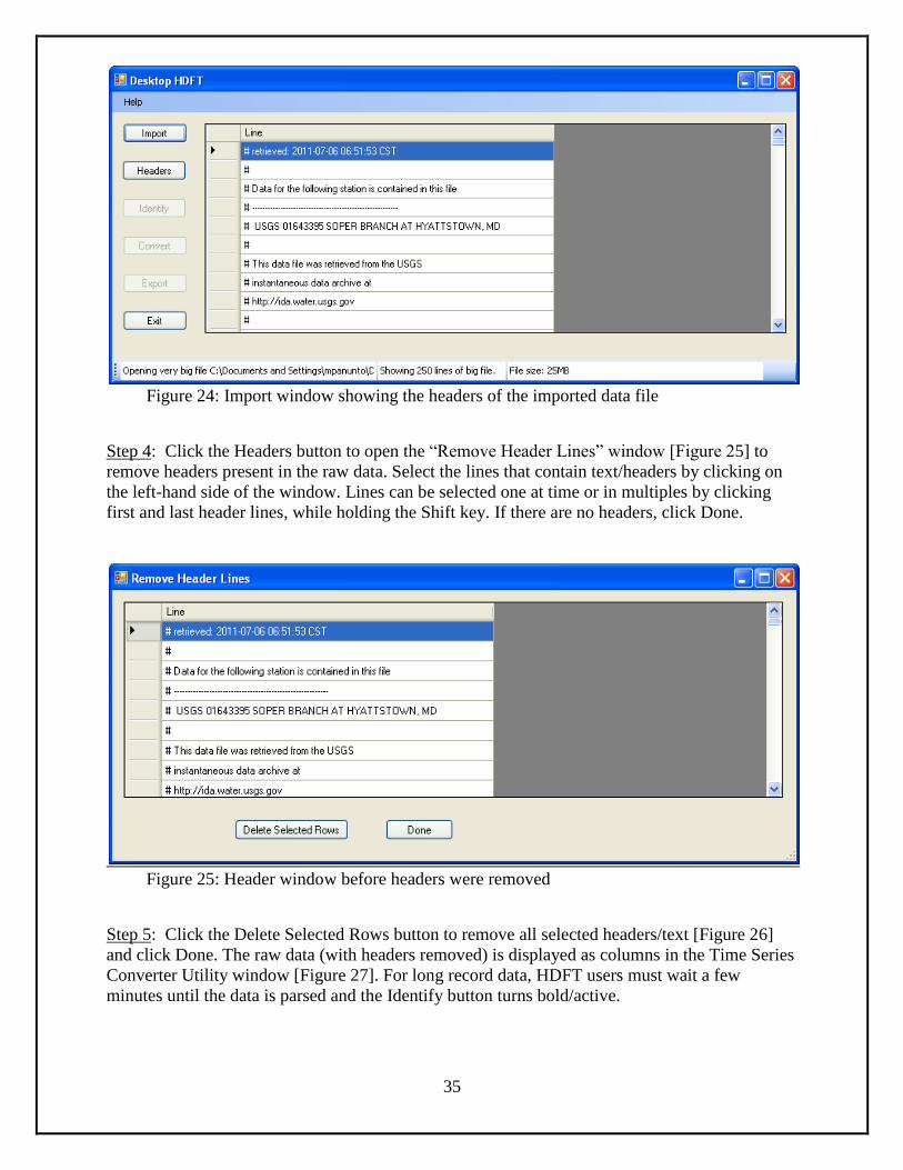
Figure 24: Import window showing the headers of the imported data file

Step 4: Click the Headers button to open the “Remove Header Lines” window [Figure 25] to

remove headers present in the raw data. Select the lines that contain text/headers by clicking on

the left-hand side of the window. Lines can be selected one at time or in multiples by clicking

first and last header lines, while holding the Shift key. If there are no headers, click Done.

Figure 25: Header window before headers were removed

Step 5: Click the Delete Selected Rows button to remove all selected headers/text [Figure 26]

and click Done. The raw data (with headers removed) is displayed as columns in the Time Series

Converter Utility window [Figure 27]. For long record data, HDFT users must wait a few

minutes until the data is parsed and the Identify button turns bold/active.

36

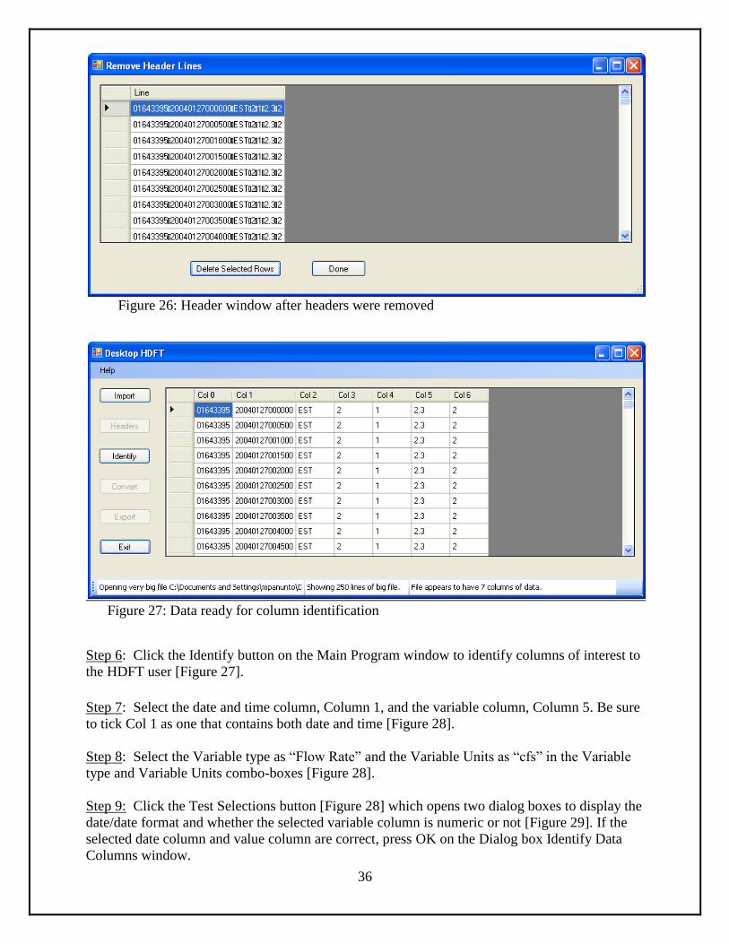
Figure 26: Header window after headers were removed

Figure 27: Data ready for column identification

Step 6: Click the Identify button on the Main Program window to identify columns of interest to

the HDFT user [Figure 27].

Step 7: Select the date and time column, Column 1, and the variable column, Column 5. Be sure

to tick Col 1 as one that contains both date and time [Figure 28].

Step 8: Select the Variable type as “Flow Rate” and the Variable Units as “cfs” in the Variable

type and Variable Units combo-boxes [Figure 28].

Step 9: Click the Test Selections button [Figure 28] which opens two dialog boxes to display the

date/date format and whether the selected variable column is numeric or not [Figure 29]. If the

selected date column and value column are correct, press OK on the Dialog box Identify Data

Columns window.

37

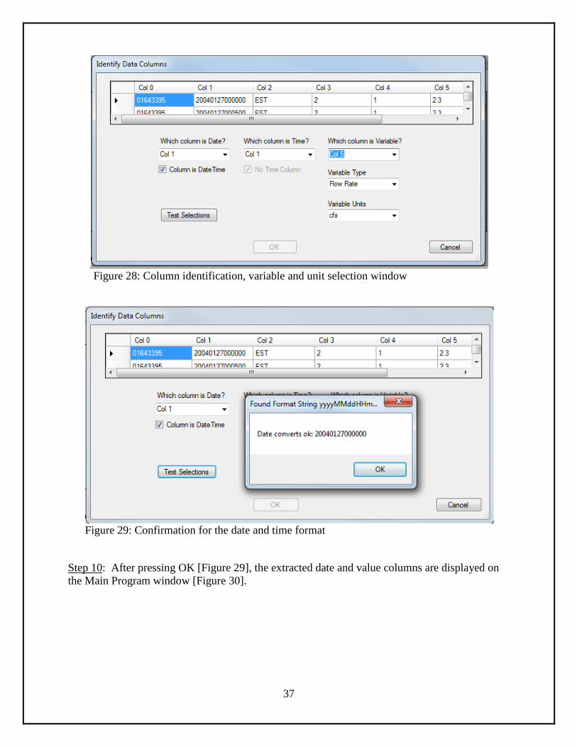
Figure 28: Column identification, variable and unit selection window

Figure 29: Confirmation for the date and time format

Step 10: After pressing OK [Figure 29], the extracted date and value columns are displayed on

the Main Program window [Figure 30].

38

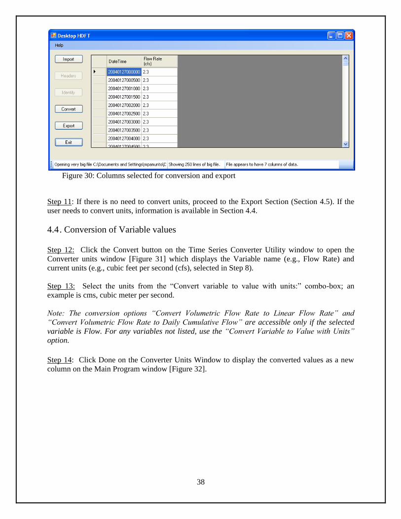
Figure 30: Columns selected for conversion and export

Step 11: If there is no need to convert units, proceed to the Export Section (Section 4.5). If the

user needs to convert units, information is available in Section 4.4.

4.4 . Conversion of Variable values

Step 12: Click the Convert button on the Time Series Converter Utility window to open the

Converter units window [Figure 31] which displays the Variable name (e.g., Flow Rate) and

current units (e.g., cubic feet per second (cfs), selected in Step 8).

Step 13: Select the units from the “Convert variable to value with units:” combo-box; an

example is cms, cubic meter per second.

Note: The conversion options “Convert Volumetric Flow Rate to Linear Flow Rate” and

“Convert Volumetric Flow Rate to Daily Cumulative Flow” are accessible only if the selected

variable is Flow. For any variables not listed, use the “Convert Variable to Value with Units”

option. Step 14: Click Done on the Converter Units Window to display the converted values as a new

column on the Main Program window [Figure 32].

39

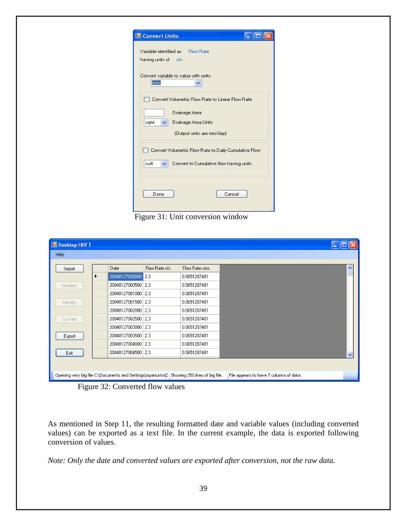
Figure 31: Unit conversion window

Figure 32: Converted flow values

As mentioned in Step 11, the resulting formatted date and variable values (including converted

values) can be exported as a text file. In the current example, the data is exported following

conversion of values.

Note: Only the date and converted values are exported after conversion, not the raw data.

40

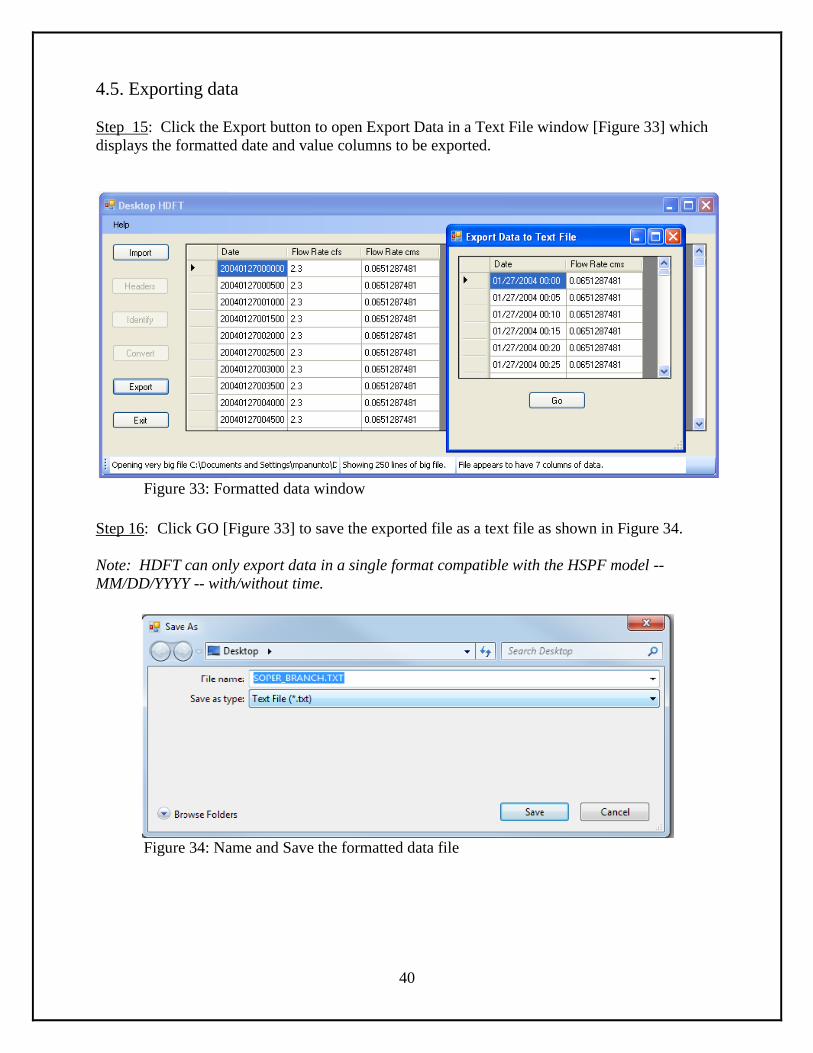
4.5. Exporting data

Step 15: Click the Export button to open Export Data in a Text File window [Figure 33] which

displays the formatted date and value columns to be exported.

Figure 33: Formatted data window

Step 16: Click GO [Figure 33] to save the exported file as a text file as shown in Figure 34.

Note: HDFT can only export data in a single format compatible with the HSPF model --

MM/DD/YYYY -- with/without time.

Figure 34: Name and Save the formatted data file

41

Chapter 5: Exporting HDFT-Formatted Data to WDMutil for HSPF

Model Use

This section provides additional information on handling various data formats, using other

resources such as the WDMUtil tool of BASINS software. For more information on the

WDMUtil tool, WDM Scripts and BASINS software, the user is referred to the following links:

WDMutil tool tutorial


BASINS Software

http://water.epa.gov/scitech/datait/models/basins/index.cfm

BASINS – Tutorials, Training and Lectures etc

http://water.epa.gov/scitech/datait/models/basins/training.cfm

Note: Chapter 5 assumes the user has a working knowledge of WDMUtil. Information about

WDMUtil can be found in BASINS training exercise #3.

Data exported from HDFT should not have headers, as WDM files require input data without

headers. To import HDFT-formatted data to a WDM file, users can use three formatting scripts

that work with one uniform date format and three time formats. The uniform date format

(MM\DD\YYYY) is made possible by using HDFT to pre-process data. HDFT exported

datafiles can have any of the following formats:

Date and time Value

Daily MM\DD\YYYY XX.XX

Hourly MM\DD\YYYY hh XX.XX

Hourly MM\DD\YYYY hh:00 XX.XX

Sub-hourly MM\DD\YYYY hh:mm XX.XX

There are separate scripts for each of the temporal resolutions and guidelines on using each .


http://water.epa.gov/scitech/datait/models/basins/index.cfm

http://water.epa.gov/scitech/datait/models/basins/training.cfm

42

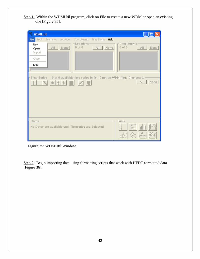
Step 1: Within the WDMUtil program, click on File to create a new WDM or open an existing

one [Figure 35].

Figure 35: WDMUtil Window

Step 2: Begin importing data using formatting scripts that work with HFDT formatted data

[Figure 36].

43

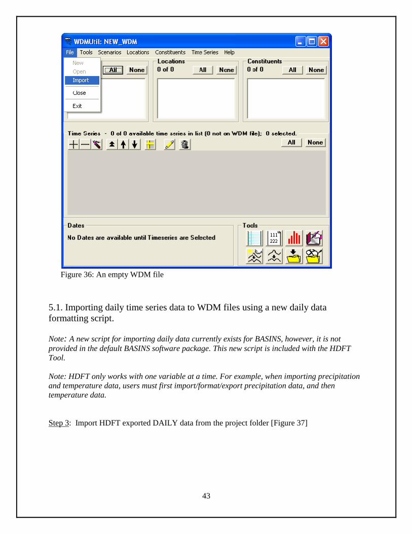
Figure 36: An empty WDM file

5.1. Importing daily time series data to WDM files using a new daily data

formatting script.

Note: A new script for importing daily data currently exists for BASINS, however, it is not

provided in the default BASINS software package. This new script is included with the HDFT

Tool.

Note: HDFT only works with one variable at a time. For example, when importing precipitation

and temperature data, users must first import/format/export precipitation data, and then

temperature data.

Step 3: Import HDFT exported DAILY data from the project folder [Figure 37]

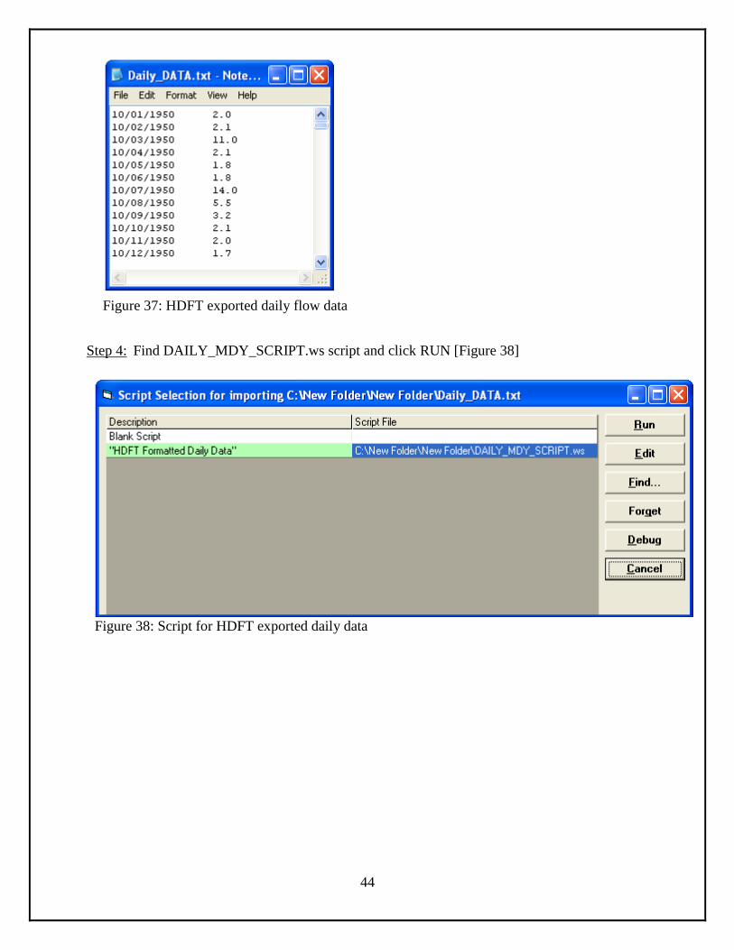
44

Figure 37: HDFT exported daily flow data

Step 4: Find DAILY_MDY_SCRIPT.ws script and click RUN [Figure 38]

Figure 38: Script for HDFT exported daily data

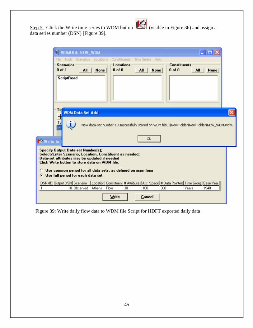
45

Step 5: Click the Write time-series to WDM button (visible in Figure 36) and assign a

data series number (DSN) [Figure 39].

Figure 39: Write daily flow data to WDM file Script for HDFT exported daily data

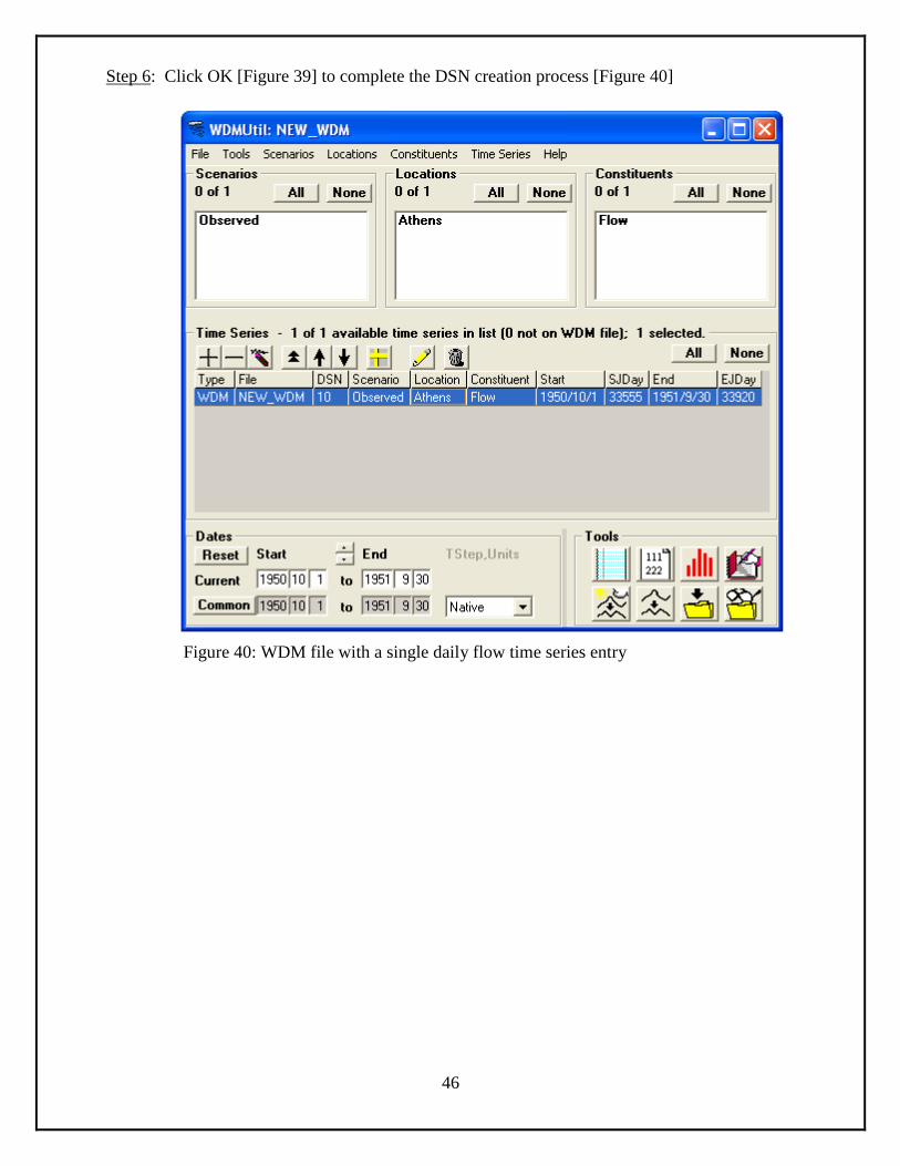
46

Step 6: Click OK [Figure 39] to complete the DSN creation process [Figure 40]

Figure 40: WDM file with a single daily flow time series entry

47

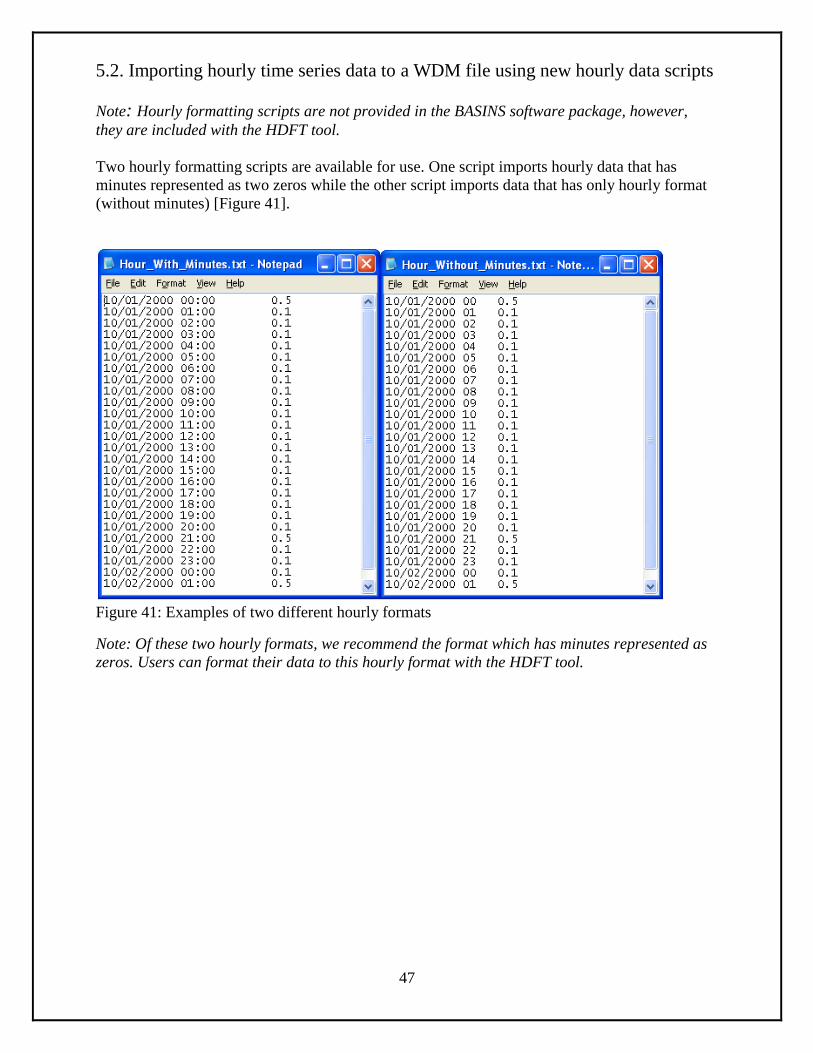
5.2. Importing hourly time series data to a WDM file using new hourly data scripts

Note: Hourly formatting scripts are not provided in the BASINS software package, however,

they are included with the HDFT tool.

Two hourly formatting scripts are available for use. One script imports hourly data that has

minutes represented as two zeros while the other script imports data that has only hourly format

(without minutes) [Figure 41].

Figure 41: Examples of two different hourly formats

Note: Of these two hourly formats, we recommend the format which has minutes represented as

zeros. Users can format their data to this hourly format with the HDFT tool.

48

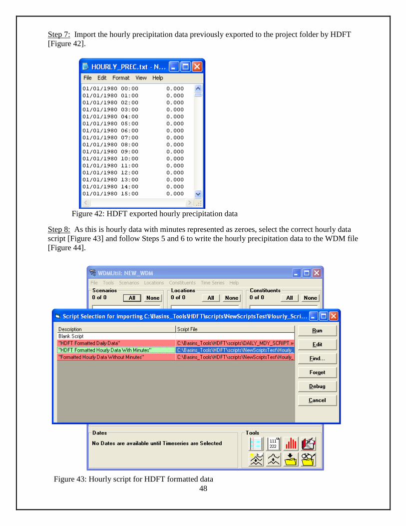
Step 7: Import the hourly precipitation data previously exported to the project folder by HDFT

[Figure 42].

Figure 42: HDFT exported hourly precipitation data

Step 8: As this is hourly data with minutes represented as zeroes, select the correct hourly data

script [Figure 43] and follow Steps 5 and 6 to write the hourly precipitation data to the WDM file

[Figure 44].

Figure 43: Hourly script for HDFT formatted data

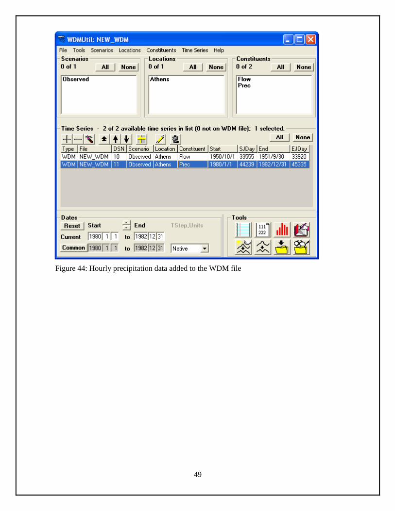
49

Figure 44: Hourly precipitation data added to the WDM file

50

5.3. Importing sub-hourly time series data to a WDM file, using a new sub-hourly

data script

Note: A sub-hourly formatting script is not provided in the default BASINS software package,

however, this script is included with the tool.

Step 9: Import sub-hourly HDFT exported data from the project folder [Figure 45]

Figure 45: HDFT exported sub-hourly (5 minute interval) flow data

51

Step 10: Select the sub-hourly data script [Figure 46] and follow Steps 5 and 6 to write the sub-

hourly data to the WDM file.

Figure 46: Sub-hourly script for HDFT formatted data

Note: The sub-hourly data shifts back one time step when imported into the WDM program. For

example, a date starting at midnight will shift back to the day before, i.e., 2004-10-01 00:00 will

shift to 2003-09-30 23:55. Step 11 corrects this problem.

Step 11: Click on List/Edit Time Series Button (visible in Figure 44) and under the File

tab click New Time Series. Once the New Time Series window is open, specify the sub-hourly

time step of the data on the Change Interval Tab [Figure 47].

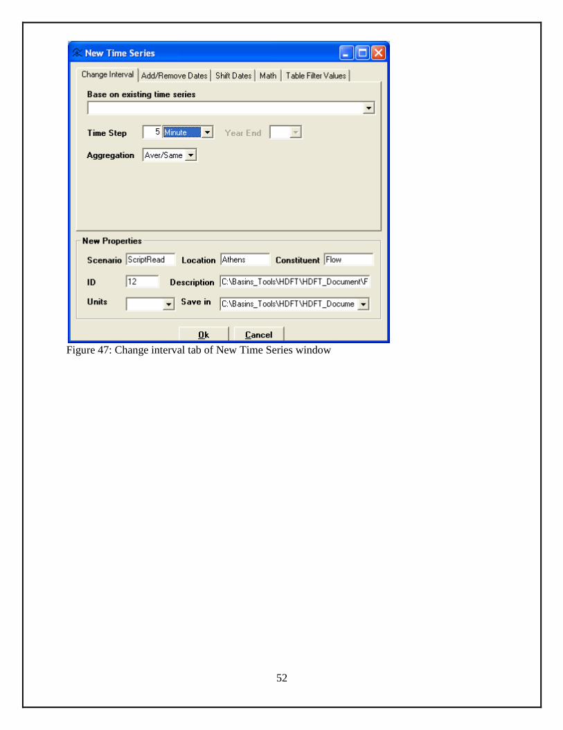
52

Figure 47: Change interval tab of New Time Series window

53

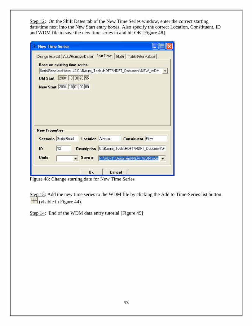
Step 12: On the Shift Dates tab of the New Time Series window, enter the correct starting

date/time next into the New Start entry boxes. Also specify the correct Location, Constituent, ID

and WDM file to save the new time series in and hit OK [Figure 48].

Figure 48: Change starting date for New Time Series

Step 13: Add the new time series to the WDM file by clicking the Add to Time-Series list button

(visible in Figure 44).

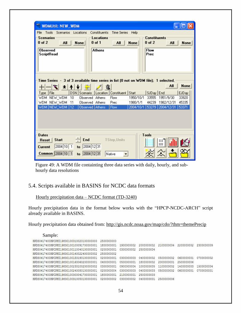
Step 14: End of the WDM data entry tutorial [Figure 49]

54

Figure 49: A WDM file containting three data series with daily, hourly, and sub-

hourly data resolutions

5.4. Scripts available in BASINS for NCDC data formats

Hourly precipitation data – NCDC format (TD-3240)

Hourly precipitation data in the format below works with the “HPCP-NCDC-ARCH” script

already available in BASINS.

Hourly precipitation data obtained from: http://gis.ncdc.noaa.gov/map/cdo/?thm=themePrecip

Sample:

http://gis.ncdc.noaa.gov/map/cdo/?thm=themePrecip

55

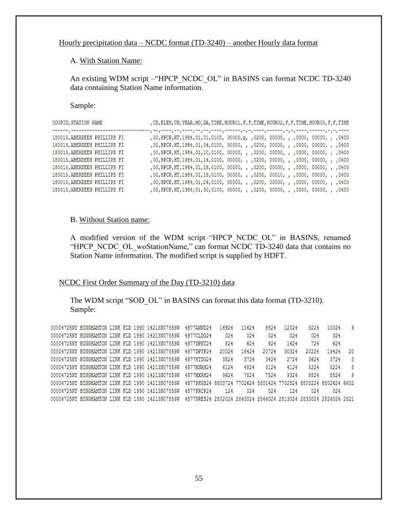
Hourly precipitation data – NCDC format (TD-3240) – another Hourly data format

A. With Station Name:

An existing WDM script –“HPCP_NCDC_OL” in BASINS can format NCDC TD-3240

data containing Station Name information.

Sample:

B. Without Station name:

A modified version of the WDM script–“HPCP_NCDC_OL” in BASINS, renamed

“HPCP_NCDC_OL_woStationName,” can format NCDC TD-3240 data that contains no

Station Name information. The modified script is supplied by HDFT.

NCDC First Order Summary of the Day (TD-3210) data

The WDM script “SOD_OL” in BASINS can format this data format (TD-3210).

Sample:

56

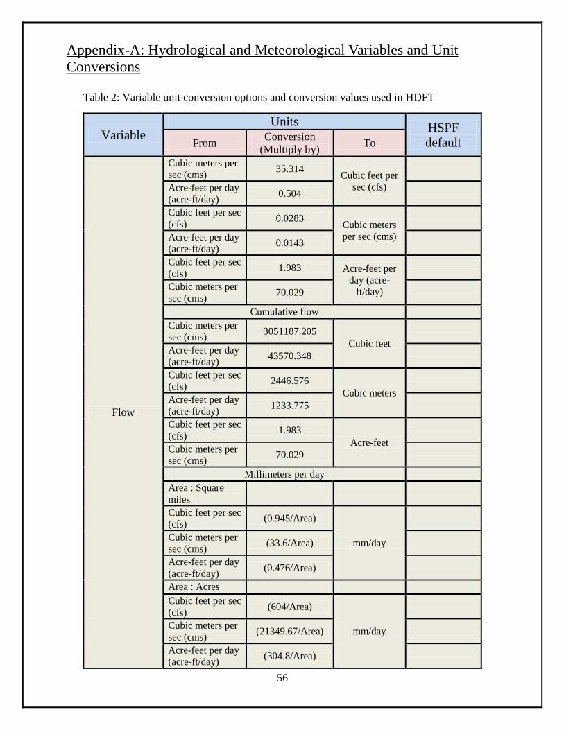
Appendix-A: Hydrological and Meteorological Variables and Unit

Conversions

Table 2: Variable unit conversion options and conversion values used in HDFT

Variable Units

HSPF

default From Conversion

(Multiply by) To

Flow

Cubic meters per

sec (cms) 35.314

Cubic feet per

sec (cfs)

Acre-feet per day

(acre-ft/day) 0.504

Cubic feet per sec

(cfs) 0.0283

Cubic meters

per sec (cms)

Acre-feet per day

(acre-ft/day) 0.0143

Cubic feet per sec

(cfs) 1.983 Acre-feet per

day (acre-

ft/day)

Cubic meters per

sec (cms) 70.029

Cumulative flow

Cubic meters per

sec (cms) 3051187.205

Cubic feet

Acre-feet per day

(acre-ft/day) 43570.348

Cubic feet per sec

(cfs) 2446.576

Cubic meters

Acre-feet per day

(acre-ft/day) 1233.775

Cubic feet per sec

(cfs) 1.983

Acre-feet

Cubic meters per

sec (cms) 70.029

Millimeters per day

Area : Square

miles

Cubic feet per sec

(cfs) (0.945/Area)

mm/day

Cubic meters per

sec (cms) (33.6/Area)

Acre-feet per day

(acre-ft/day) (0.476/Area)

Area : Acres

Cubic feet per sec

(cfs) (604/Area)

mm/day

Cubic meters per


Acre-feet per day


57

Area : Square

Kilometers

Cubic feet per sec

(cfs) (2.447/Area)

mm/day

Cubic meters per


Acre-feet per day


Concentration

Micrograms per

liter (µg/l) 0.001

Milligrams per

liter (mg/L)

Milligrams per

liter (mg/L) 1000

Micrograms

per liter (µg/l)

Load

Kilograms per

day (Kg/day) 2.208

Pounds/day

(Lb/day)

Tonnes per day

(Tonnes/day) 2204.622

Kilogram per

second (Kg/sec) 190728.477

Pounds/day

(Lb/day) 0.453

Kilograms per

day (Kg/day)

Tonnes per day

(Tonnes/day) 1000

Kilograms per

second (Kg/sec) 86400

Pounds/day

(Lb/day) 0.000045

Tonnes per

day

(Tonnes/day)

Kilograms per

day (Kg/day) 0.001

Kilograms per

second (Kg/sec) 86.4

Pounds/day

(Lb/day) 5.243×10

-6

Kilograms per

second

(Kg/sec)

Kilograms per

day (Kg/day) 0.0000115

Tonnes per day

(Tonnes/day) 0.1157

Precipitation

Inches per hour

(Inches/hr) 25.4 Millimeters

per hour

(mm/hr) Inches per hour

(Inches/hr) Millimeters per

hour (mm/hr) 0.0393 Inches per

hour

(Inches/hr)

Temperature Centigrade (

0C) [9*(

0C)/5]+32 Fahrenheit (

0F)

Fahrenheit (0F) Fahrenheit (

0F)

[5*(0C)/9]-32

Centigrade

(0C)

Solar Radiation

Watts per square

meter (Watt/m2)

0.0858

Langley per

hour

(Langley/hr)

Langley per

hour

(Langley/hr)

Cloud Cover Oktas (1 to 10) --------- Oktas (1 to 10) Oktas (1 to 10)

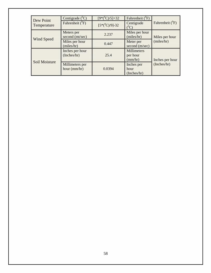
58

Dew Point

Temperature

Centigrade (0C) [9*(

0C)/5]+32 Fahrenheit (

0F)

Fahrenheit (0F) Fahrenheit (

0F)

[5*(0C)/9]-32

Centigrade

(0C)

Wind Speed

Meters per

second (mt/sec) 2.237

Miles per hour

(miles/hr) Miles per hour

(miles/hr) Miles per hour

(miles/hr) 0.447

Meter per

second (m/sec)

Soil Moisture

Inches per hour

(Inches/hr) 25.4 Millimeters

per hour

(mm/hr) Inches per hour

(Inches/hr) Millimeters per

hour (mm/hr) 0.0394

Inches per

hour

(Inches/hr)

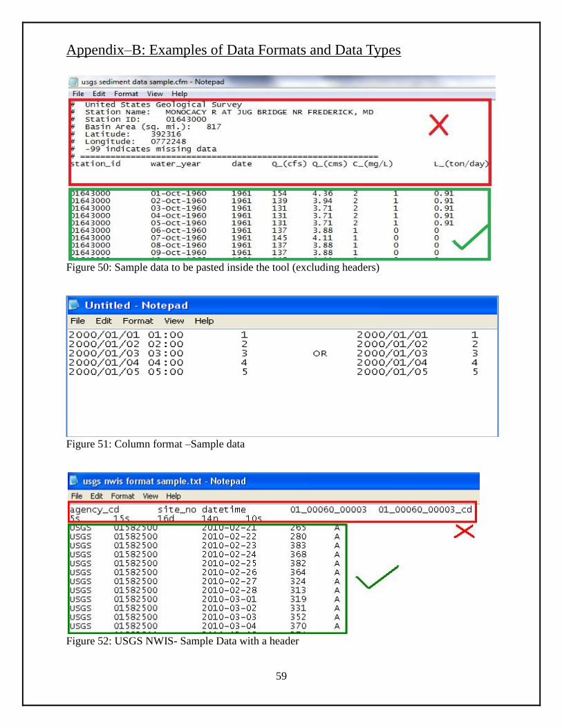
59

Appendix–B: Examples of Data Formats and Data Types

Figure 50: Sample data to be pasted inside the tool (excluding headers)

Figure 51: Column format –Sample data

Figure 52: USGS NWIS- Sample Data with a header

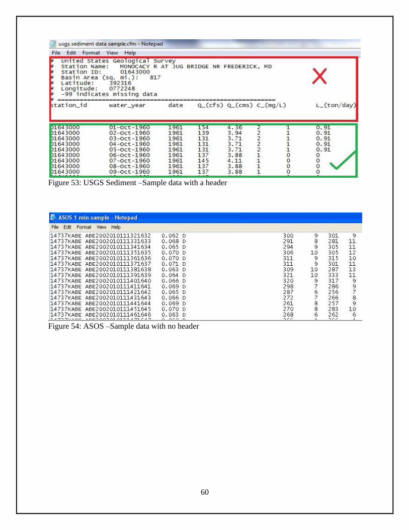
60

Figure 53: USGS Sediment –Sample data with a header

Figure 54: ASOS –Sample data with no header

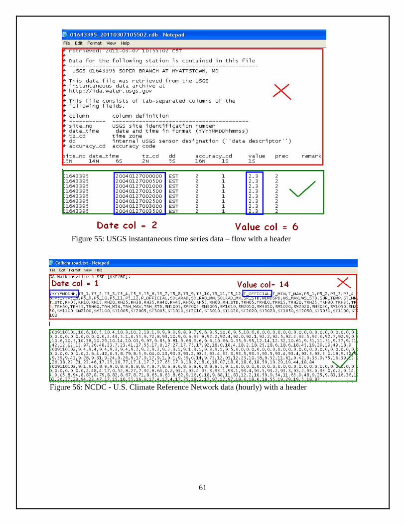
61

Figure 55: USGS instantaneous time series data – flow with a header

Figure 56: NCDC - U.S. Climate Reference Network data (hourly) with a header

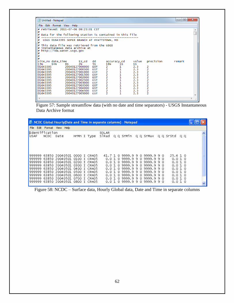
62

Figure 57: Sample streamflow data (with no date and time separators) - USGS Instantaneous

Data Archive format

Figure 58: NCDC – Surface data, Hourly Global data, Date and Time in separate columns

63

Appendix-C: Downloading Data from the National Climate Data Center

NCDC: * National Climatic Data Center (NCDC) *

www.ncdc.noaa.gov/

Figure 59: National Climatic Data Center home page

To access data, follow these steps:

Step 1: Click on the “Climate Data Online” link [Figure 59] to open an interactive map

application web page [Figure 60].

Step 2: Click on the “Interactive Map Application” figure to open an interactive GIS-based

world map. Initially, a help window displays to provide information on downloading the data

[Figure 61].

Step 3: Close the Map Help window to view the world map [Figure 62].

http://www.ncdc.noaa.gov/

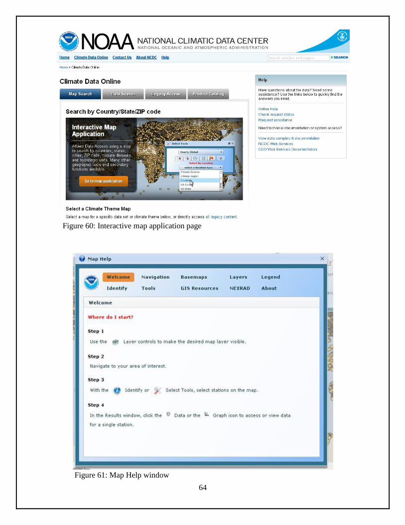
64

Figure 60: Interactive map application page

Figure 61: Map Help window

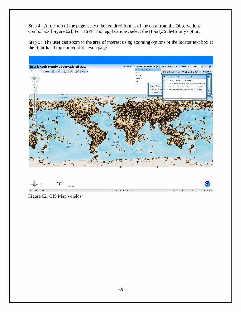
65

Step 4: At the top of the page, select the required format of the data from the Observations

combo box [Figure 62]. For HSPF Tool applications, select the Hourly/Sub-Hourly option.

Step 5: The user can zoom to the area of interest using zooming options or the locator text box at

the right-hand top corner of the web page.

Figure 62: GIS Map window

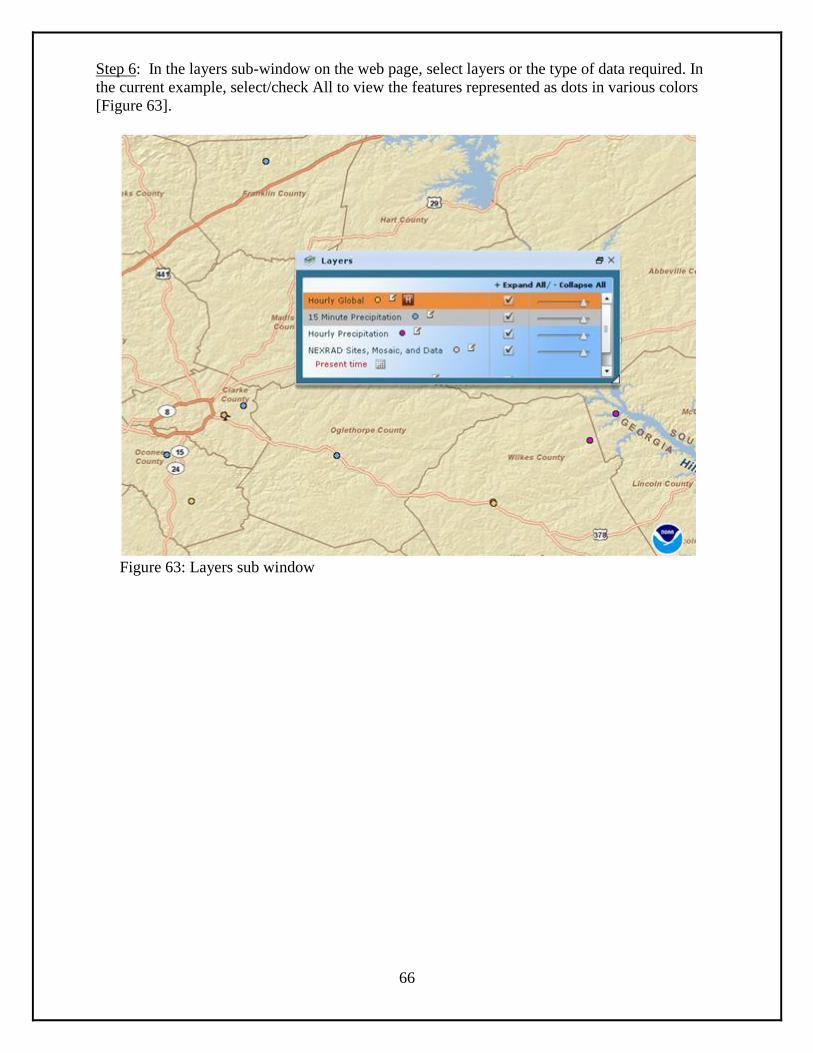
66

Step 6: In the layers sub-window on the web page, select layers or the type of data required. In

the current example, select/check All to view the features represented as dots in various colors

[Figure 63].

Figure 63: Layers sub window

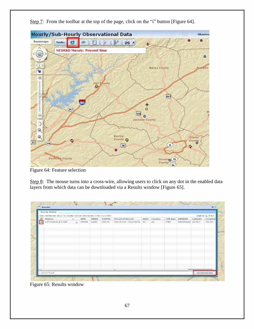
67

Step 7: From the toolbar at the top of the page, click on the “i” button [Figure 64].

Figure 64: Feature selection

Step 8: The mouse turns into a cross-wire, allowing users to click on any dot in the enabled data

layers from which data can be downloaded via a Results window [Figure 65].

Figure 65: Results window

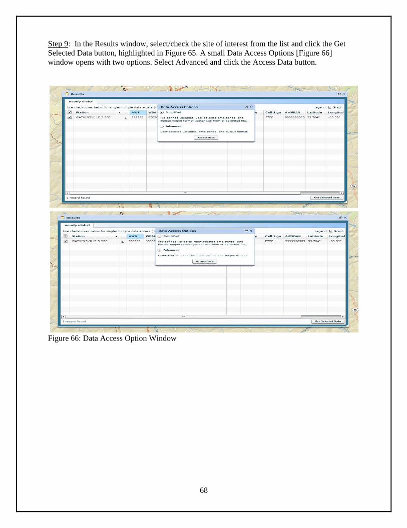
68

Step 9: In the Results window, select/check the site of interest from the list and click the Get

Selected Data button, highlighted in Figure 65. A small Data Access Options [Figure 66]

window opens with two options. Select Advanced and click the Access Data button.

Figure 66: Data Access Option Window

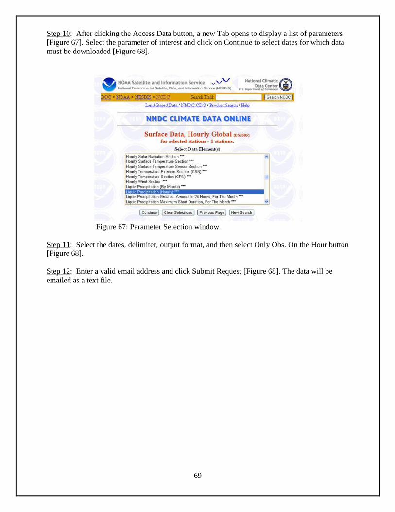
69

Step 10: After clicking the Access Data button, a new Tab opens to display a list of parameters

[Figure 67]. Select the parameter of interest and click on Continue to select dates for which data

must be downloaded [Figure 68].

Figure 67: Parameter Selection window

Step 11: Select the dates, delimiter, output format, and then select Only Obs. On the Hour button

[Figure 68].

Step 12: Enter a valid email address and click Submit Request [Figure 68]. The data will be

emailed as a text file.

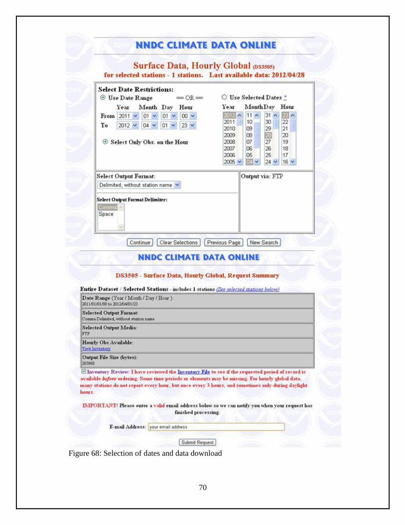
70

Figure 68: Selection of dates and data download

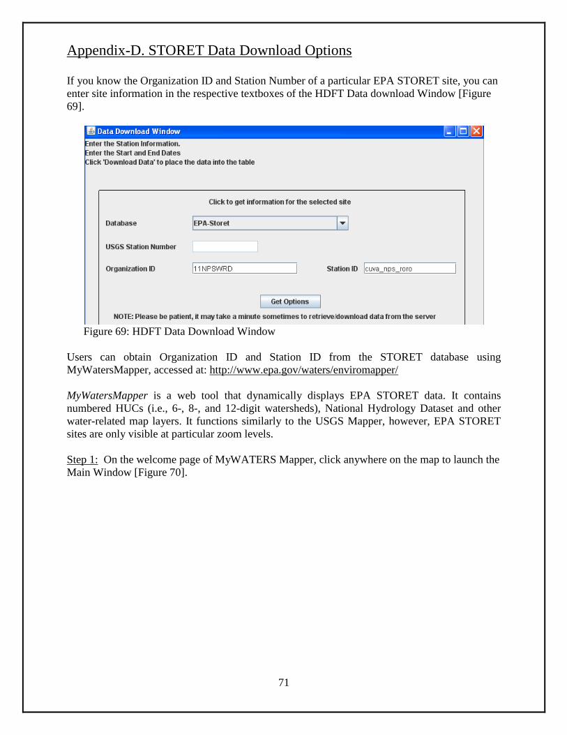
71

Appendix-D. STORET Data Download Options

If you know the Organization ID and Station Number of a particular EPA STORET site, you can

enter site information in the respective textboxes of the HDFT Data download Window [Figure

69].

Figure 69: HDFT Data Download Window

Users can obtain Organization ID and Station ID from the STORET database using

MyWatersMapper, accessed at: http://www.epa.gov/waters/enviromapper/

MyWatersMapper is a web tool that dynamically displays EPA STORET data. It contains

numbered HUCs (i.e., 6-, 8-, and 12-digit watersheds), National Hydrology Dataset and other

water-related map layers. It functions similarly to the USGS Mapper, however, EPA STORET

sites are only visible at particular zoom levels.

Step 1: On the welcome page of MyWATERS Mapper, click anywhere on the map to launch the

Main Window [Figure 70].

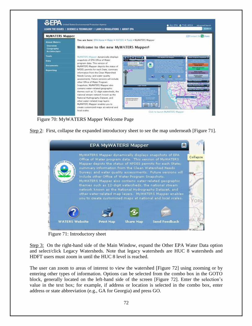
http://www.epa.gov/waters/enviromapper/

72

Figure 70: MyWATERS Mapper Welcome Page

Step 2: First, collapse the expanded introductory sheet to see the map underneath [Figure 71].

Figure 71: Introductory sheet

Step 3: On the right-hand side of the Main Window, expand the Other EPA Water Data option

and select/click Legacy Watersheds. Note that legacy watersheds are HUC 8 watersheds and

HDFT users must zoom in until the HUC 8 level is reached.

The user can zoom to areas of interest to view the watershed [Figure 72] using zooming or by

entering other types of information. Options can be selected from the combo box in the GOTO

block, generally located on the left-hand side of the screen [Figure 72]. Enter the selection’s

value in the text box; for example, if address or location is selected in the combo box, enter

address or state abbreviation (e.g., GA for Georgia) and press GO.

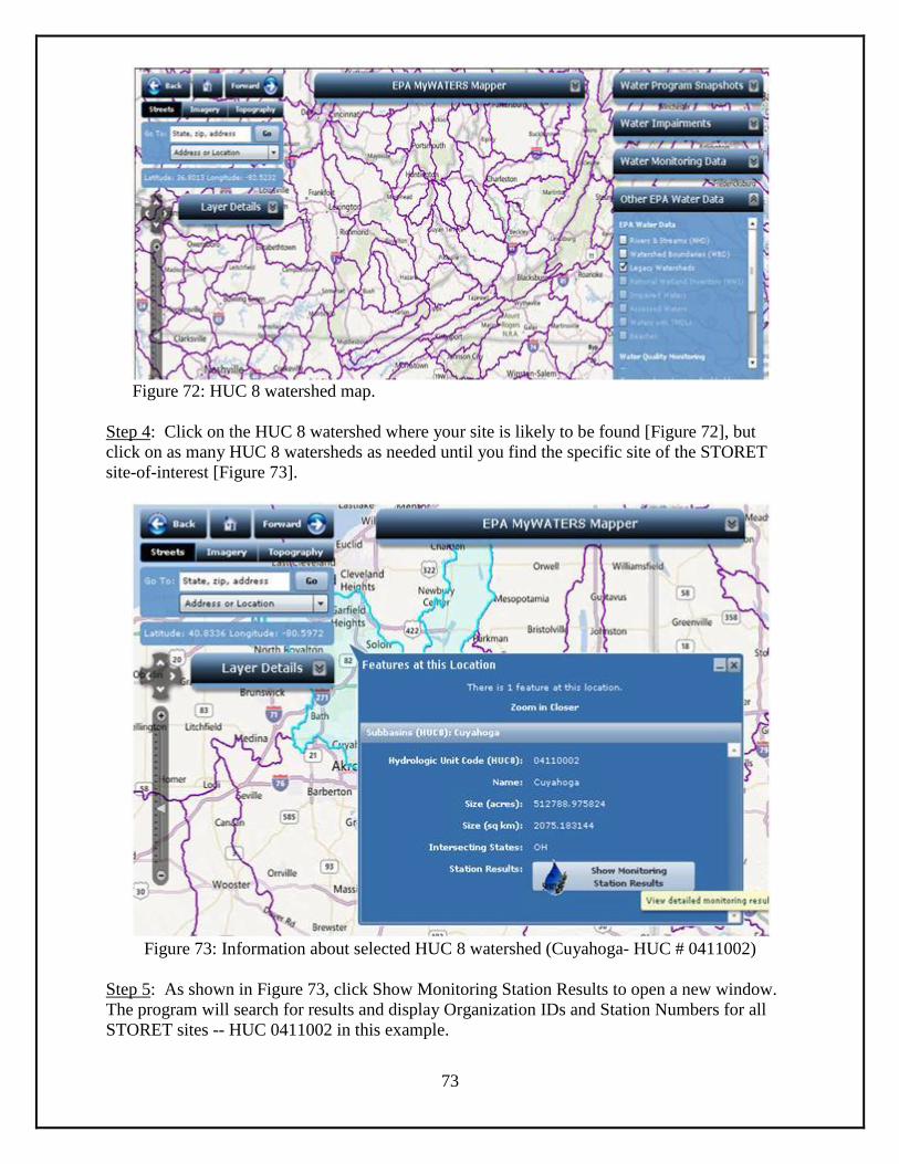
73

Figure 72: HUC 8 watershed map.

Step 4: Click on the HUC 8 watershed where your site is likely to be found [Figure 72], but

click on as many HUC 8 watersheds as needed until you find the specific site of the STORET

site-of-interest [Figure 73].

Figure 73: Information about selected HUC 8 watershed (Cuyahoga- HUC # 0411002)

Step 5: As shown in Figure 73, click Show Monitoring Station Results to open a new window.

The program will search for results and display Organization IDs and Station Numbers for all

STORET sites -- HUC 0411002 in this example.

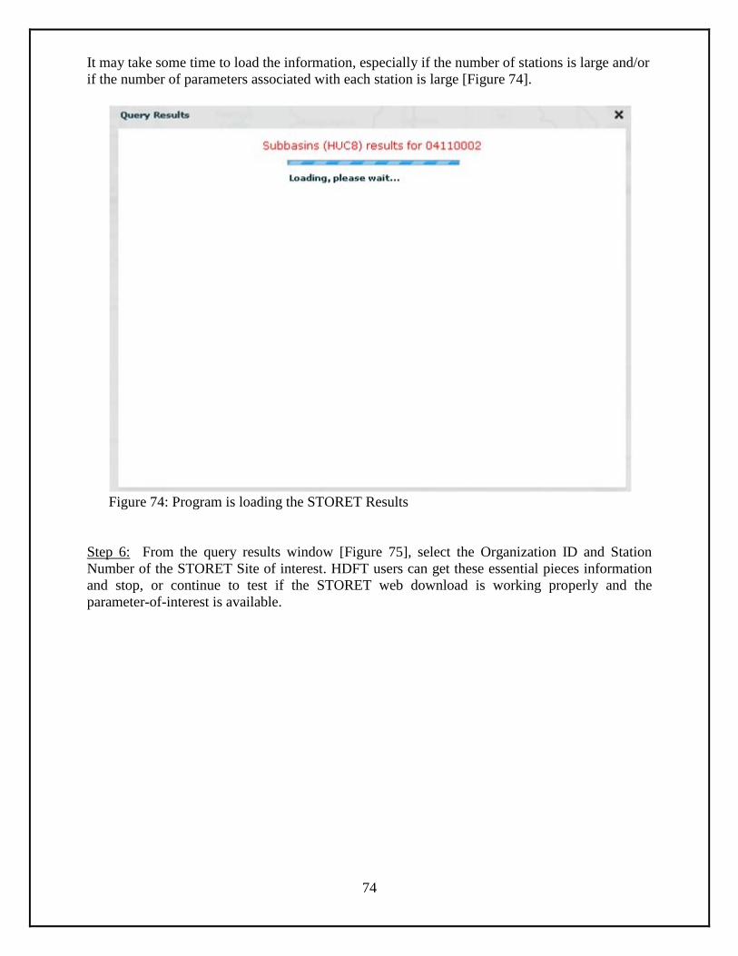
74

It may take some time to load the information, especially if the number of stations is large and/or

if the number of parameters associated with each station is large [Figure 74].

Figure 74: Program is loading the STORET Results

Step 6: From the query results window [Figure 75], select the Organization ID and Station

Number of the STORET Site of interest. HDFT users can get these essential pieces information

and stop, or continue to test if the STORET web download is working properly and the

parameter-of-interest is available.

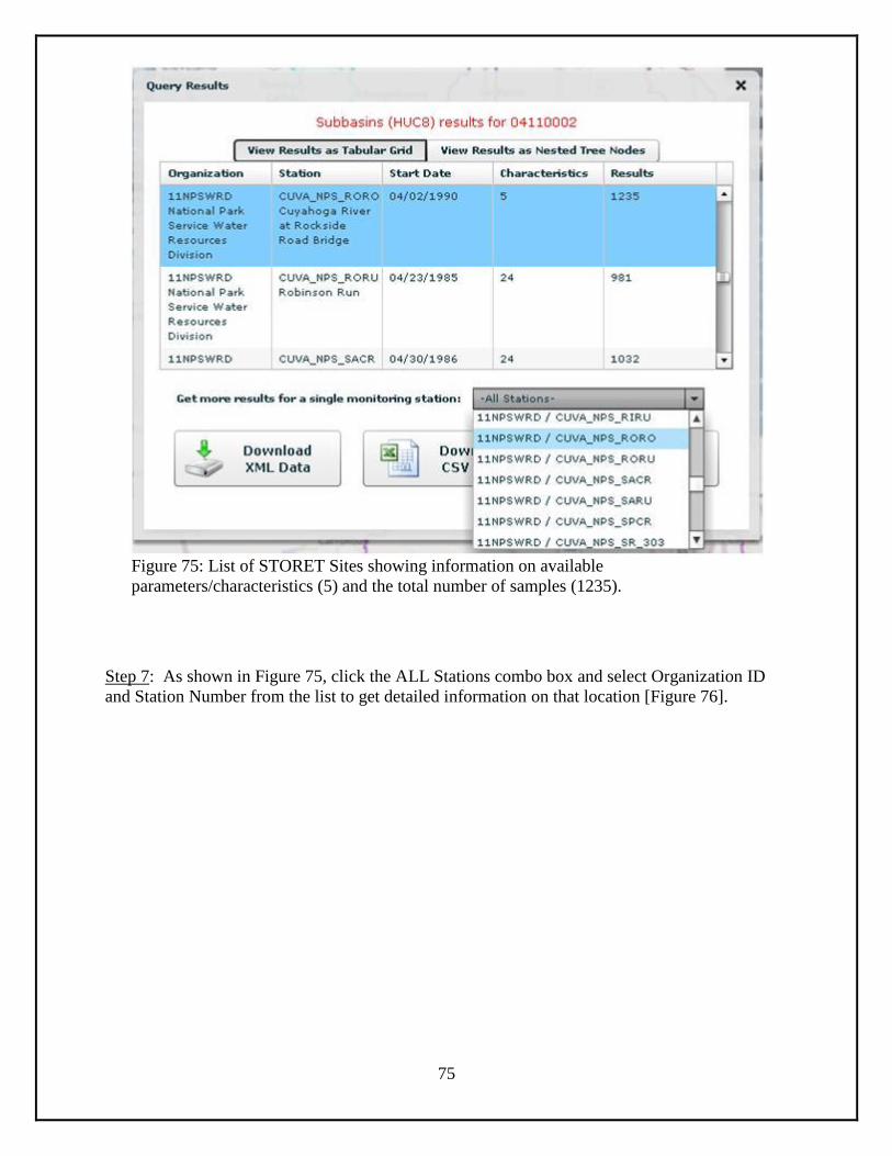
75

Figure 75: List of STORET Sites showing information on available

parameters/characteristics (5) and the total number of samples (1235).

Step 7: As shown in Figure 75, click the ALL Stations combo box and select Organization ID

and Station Number from the list to get detailed information on that location [Figure 76].

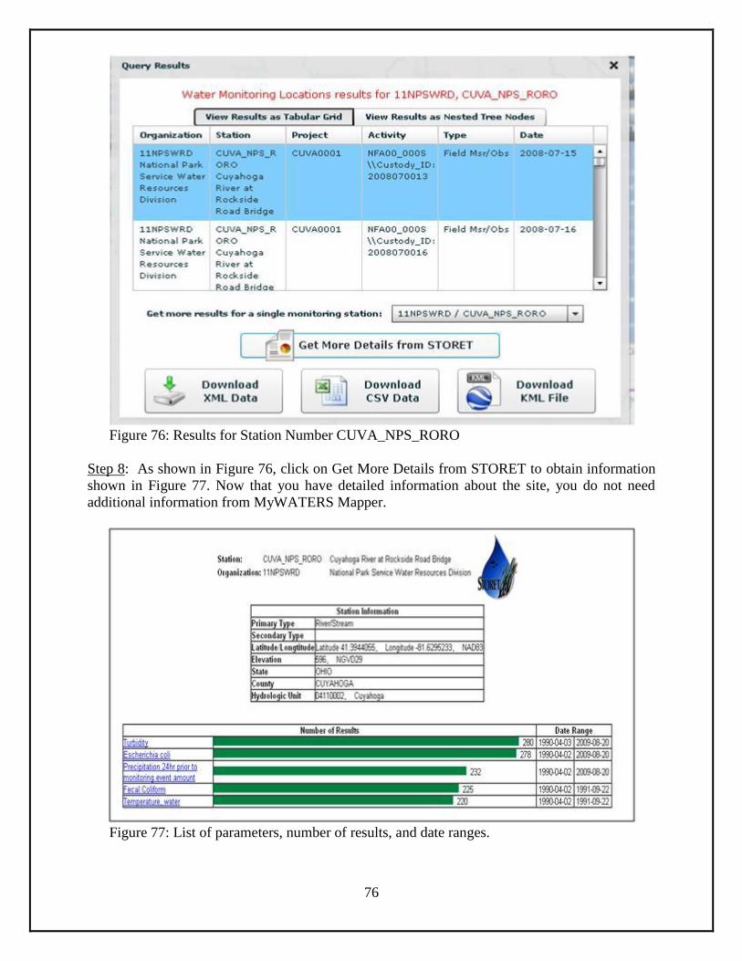
76

Figure 76: Results for Station Number CUVA_NPS_RORO

Step 8: As shown in Figure 76, click on Get More Details from STORET to obtain information

shown in Figure 77. Now that you have detailed information about the site, you do not need

additional information from MyWATERS Mapper.

Figure 77: List of parameters, number of results, and date ranges.

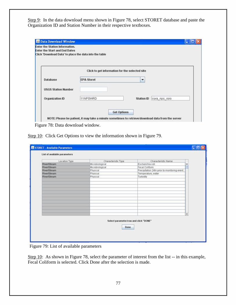
77

Step 9: In the data download menu shown in Figure 78, select STORET database and paste the

Organization ID and Station Number in their respective textboxes.

Figure 78: Data download window.

Step 10: Click Get Options to view the information shown in Figure 79.

Figure 79: List of available parameters

Step 10: As shown in Figure 78, select the parameter of interest from the list -- in this example,

Fecal Coliform is selected. Click Done after the selection is made.

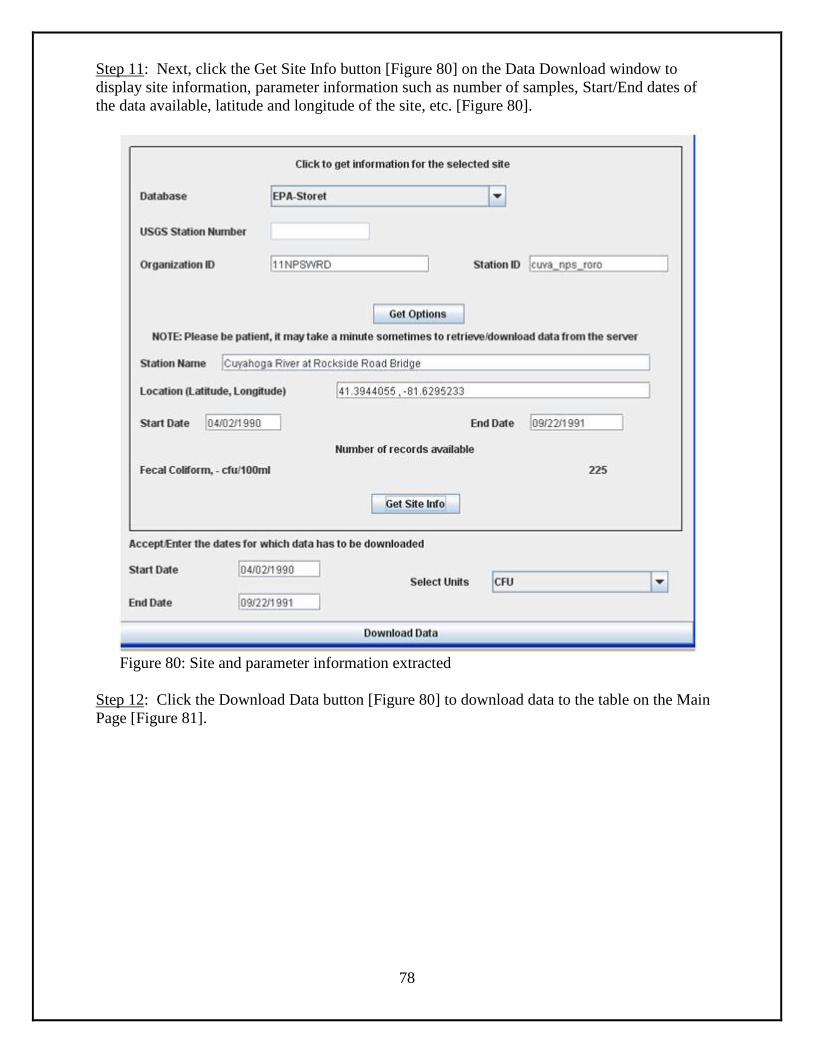
78

Step 11: Next, click the Get Site Info button [Figure 80] on the Data Download window to

display site information, parameter information such as number of samples, Start/End dates of

the data available, latitude and longitude of the site, etc. [Figure 80].

Figure 80: Site and parameter information extracted

Step 12: Click the Download Data button [Figure 80] to download data to the table on the Main

Page [Figure 81].

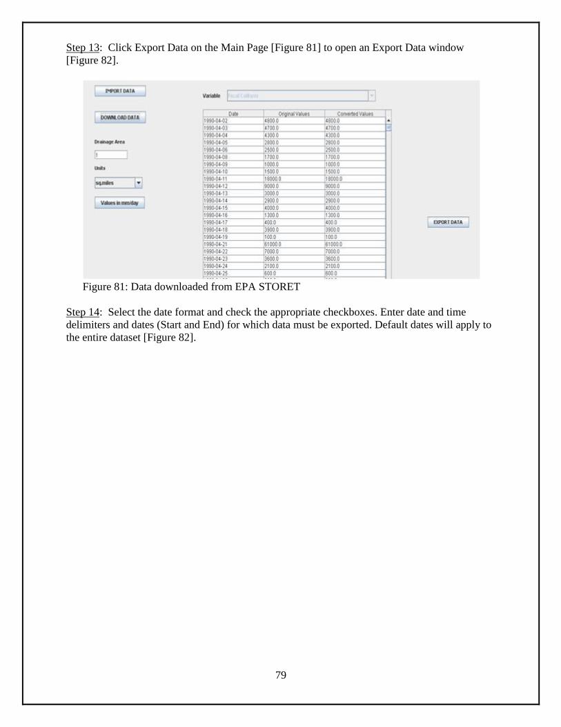
79

Step 13: Click Export Data on the Main Page [Figure 81] to open an Export Data window

[Figure 82].

Figure 81: Data downloaded from EPA STORET

Step 14: Select the date format and check the appropriate checkboxes. Enter date and time

delimiters and dates (Start and End) for which data must be exported. Default dates will apply to

the entire dataset [Figure 82].

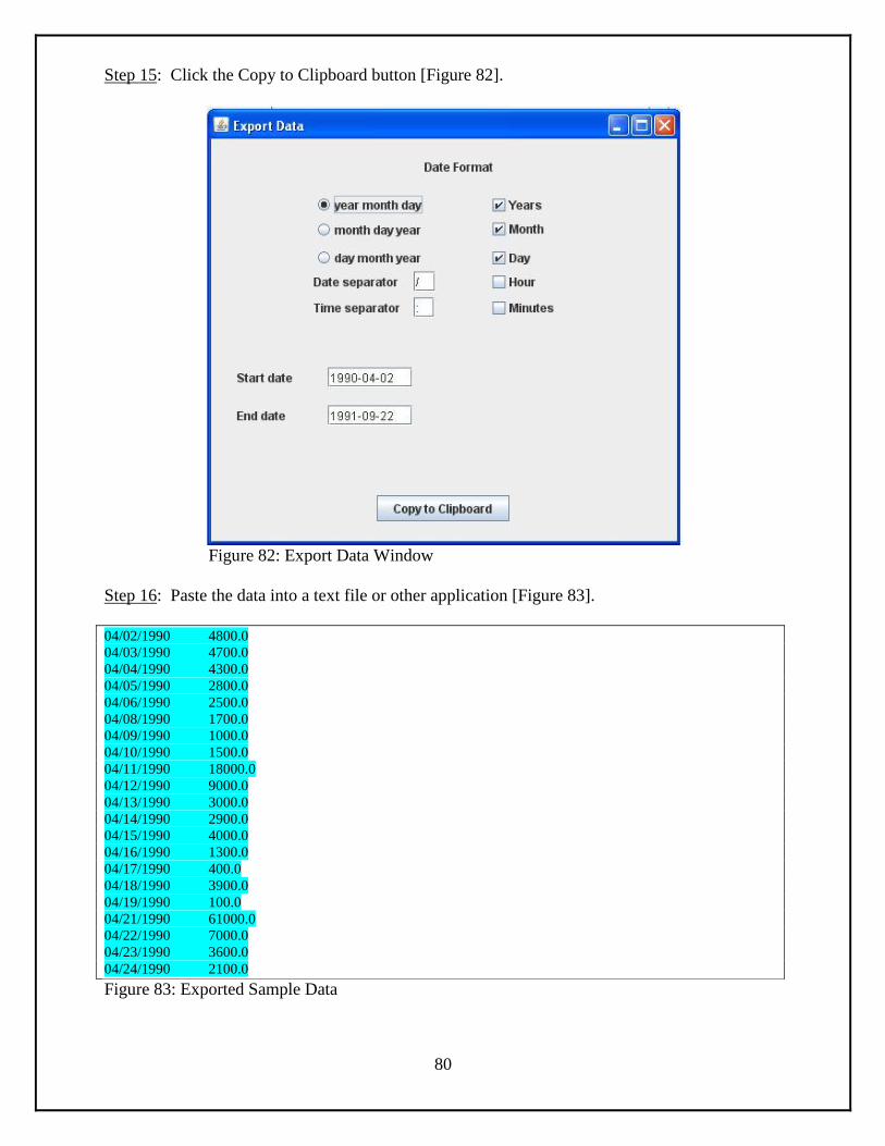
80

Step 15: Click the Copy to Clipboard button [Figure 82].

Figure 82: Export Data Window

Step 16: Paste the data into a text file or other application [Figure 83].

04/02/1990 4800.0

04/03/1990 4700.0

04/04/1990 4300.0

04/05/1990 2800.0

04/06/1990 2500.0

04/08/1990 1700.0

04/09/1990 1000.0

04/10/1990 1500.0

04/11/1990 18000.0

04/12/1990 9000.0

04/13/1990 3000.0

04/14/1990 2900.0

04/15/1990 4000.0

04/16/1990 1300.0

04/17/1990 400.0

04/18/1990 3900.0

04/19/1990 100.0

04/21/1990 61000.0

04/22/1990 7000.0

04/23/1990 3600.0

04/24/1990 2100.0

Figure 83: Exported Sample Data

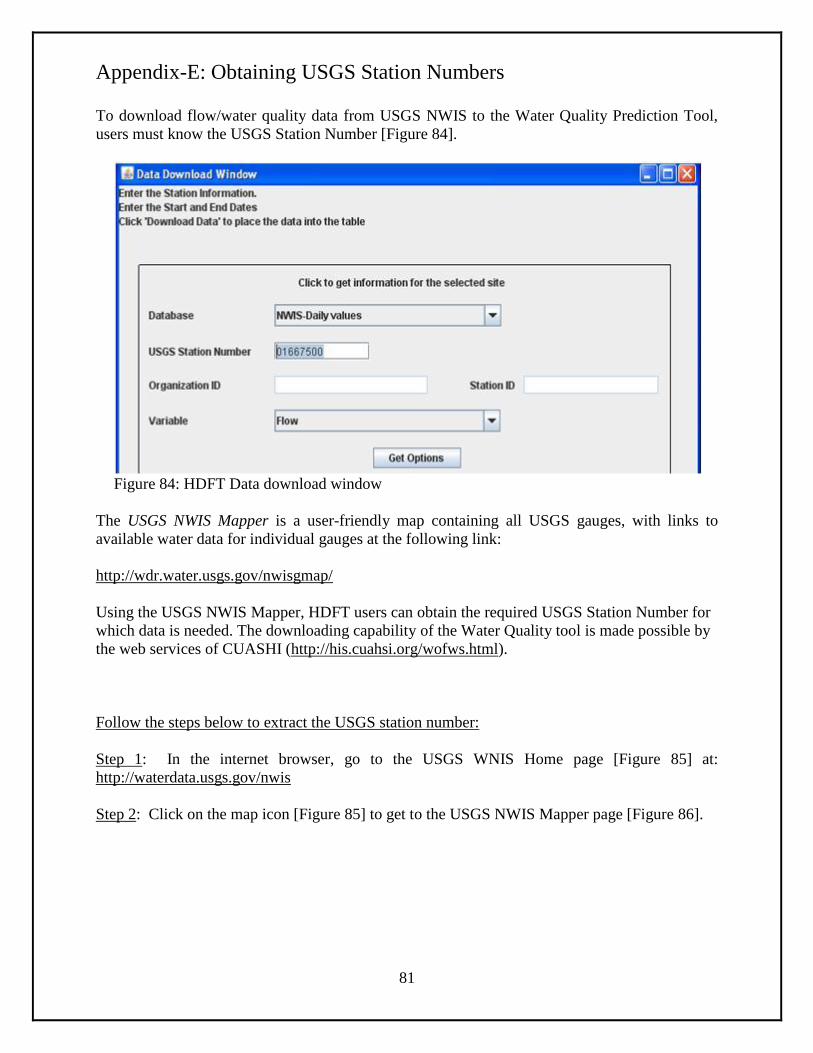
81

Appendix-E: Obtaining USGS Station Numbers

To download flow/water quality data from USGS NWIS to the Water Quality Prediction Tool,

users must know the USGS Station Number [Figure 84].

Figure 84: HDFT Data download window

The USGS NWIS Mapper is a user-friendly map containing all USGS gauges, with links to

available water data for individual gauges at the following link:

http://wdr.water.usgs.gov/nwisgmap/

Using the USGS NWIS Mapper, HDFT users can obtain the required USGS Station Number for

which data is needed. The downloading capability of the Water Quality tool is made possible by

the web services of CUASHI (http://his.cuahsi.org/wofws.html).

Follow the steps below to extract the USGS station number:

Step 1: In the internet browser, go to the USGS WNIS Home page [Figure 85] at:


Step 2: Click on the map icon [Figure 85] to get to the USGS NWIS Mapper page [Figure 86].

http://wdr.water.usgs.gov/nwisgmap/

http://his.cuahsi.org/wofws.html


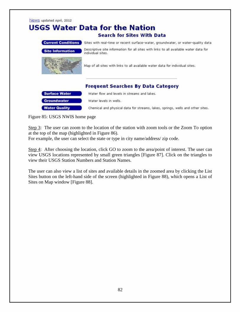
82

Figure 85: USGS NWIS home page

Step 3: The user can zoom to the location of the station with zoom tools or the Zoom To option

at the top of the map (highlighted in Figure 86).

For example, the user can select the state or type in city name/address/ zip code.

Step 4: After choosing the location, click GO to zoom to the area/point of interest. The user can

view USGS locations represented by small green triangles [Figure 87]. Click on the triangles to

view their USGS Station Numbers and Station Names.

The user can also view a list of sites and available details in the zoomed area by clicking the List

Sites button on the left-hand side of the screen (highlighted in Figure 88), which opens a List of

Sites on Map window [Figure 88].

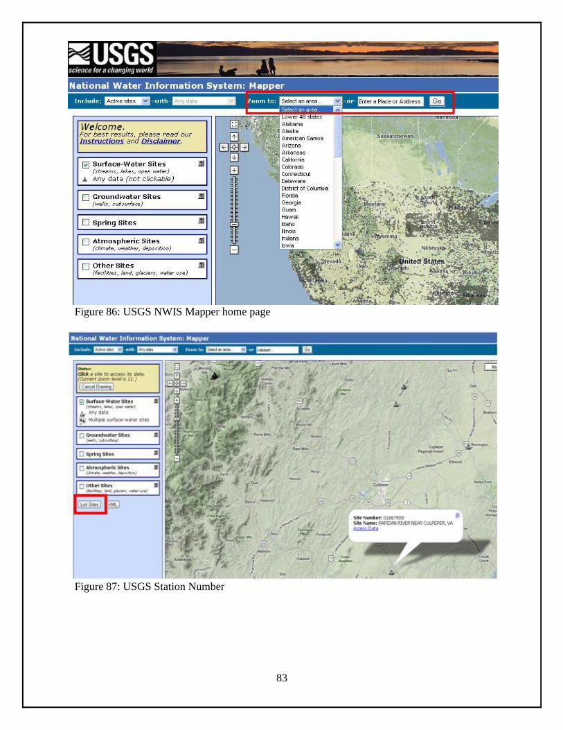
83

Figure 86: USGS NWIS Mapper home page

Figure 87: USGS Station Number

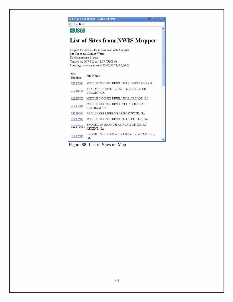
84

Figure 88: List of Sites on Map

hydrological simulation program fortran (hspf… · management of land and water resources. to meet...

Documents