hydrostatic correction for sigma coordinate ocean models

Hydrostatic correction for sigma coordinate ocean models

Peter C. Chu and Chenwu FanNaval Ocean Analysis and Prediction Laboratory, Department of Oceanography, Naval Postgraduate School, Monterey,California, USA

Received 30 September 2002; revised 17 March 2003; accepted 4 April 2003; published 27 June 2003.

[1] How to reduce the horizontal pressure gradient error is a key issue in terrain-followingcoastal models. The horizontal pressure gradient splits into two parts, and incompletecancellation of the truncation errors of those parts cause the error. Use of the finite volumediscretization leads to a conserved scheme for pressure gradient computation that hasbetter truncation properties with high accuracy. The analytical coastal topography andseamount test cases are used to evaluate the new scheme. The accuracy of the new schemeis comparable to the sixth-order combined compact scheme (with an error reduction by afactor of 70 comparing to the second-order scheme) with mild topography and muchbetter than the sixth-order combined compact scheme with steep topography. Thecomputational efficiency of the new scheme is comparable to the second-order differencescheme. The two characteristics, high accuracy and computational efficiency, makethis scheme useful for the sigma coordinate ocean models. INDEX TERMS: 4255

Oceanography: General: Numerical modeling; 4263 Oceanography: General: Ocean prediction; 4243

Oceanography: General: Marginal and semienclosed seas; 4219 Oceanography: General: Continental shelf

processes; 3337 Meteorology and Atmospheric Dynamics: Numerical modeling and data assimilation;

KEYWORDS: sigma coordinate ocean model, horizontal pressure gradient error, hydrostatic correction, finite

volume scheme, high-order scheme

Citation: Chu, P. C., and C. Fan, Hydrostatic correction for sigma coordinate ocean models, J. Geophys. Res., 108(C6), 3206,

doi:10.1029/2002JC001668, 2003.

1. Introduction

[2] In regional oceanic (or atmospheric) prediction mod-els, the effects of bottom topography must be taken intoaccount and usually the terrain-following sigma coordinatesshould be used to imply the continuous topography. Insigma coordinates the water column is divided into thesame number of grid cells regardless of the depth. Consider2D problems for mathematical simplification. Let (x, z) bethe Cartesian coordinates and (x̂, s) be the sigma coordi-nates. The conventional relationships between z and sigmacoordinates are given by

x̂ ¼ x; s ¼ z� hH þ h

; ð1Þ

where h is the surface elevation. Both z and s increasevertically upward such that z = h, s = 0 at the surface ands = �1, z = �H at the bottom. The horizontal pressuregradient becomes difference between two large terms

@p

@x¼ @p̂

@x̂� 1

H þ ss@H

@x̂þ @h

@x

� �@p̂

@s; ð2Þ

that may cause large truncation error at steep topography[e.g., Gary, 1973; Haney, 1991; Mellor et al., 1994;

McCalpin, 1994; Chu and Fan, 1997, 1998, 1999, 2000,2001; Song, 1998].[3] Several methods have been suggested to reduce the

truncation errors to acceptable levels: (1) smoothing topog-raphy [Chu and Fan, 2001], (2) subtracting a mean verticaldensity profile before calculating the gradient [Gary, 1973;Mellor et al., 1994], (3) bringing certain symmetries of thecontinuous forms into the discrete level to ensure cancella-tions of these terms such as the density Jacobian scheme[e.g., Mellor et al., 1998; Song, 1998; Song and Wright,1998], (4) increasing numerical accuracy [e.g., McCalpin,1994; Chu and Fan, 1997, 1998, 1999, 2000, 2001], (5)changing the grid from a sigma grid to a z level grid beforecalculating the horizontal pressure gradient [e.g., Stellingand van Kester, 1994]. Kliem and Pietrzak [1999] claimedthat the z level based pressure gradient calculation is themost simple and effective means to reduce the pressuregradient errors. After comparing to other schemes, Ezer etal. [2002] show the favorable performance of the latestpolynomial schemes. Recently, Shchepetkin and McWil-liams [2002] design a pressure gradient algorithm withsplines that achieves more accurate hydrostatic balancebetween the two components and that does not lose asmuch accuracy with nonuniform vertical grids at relativelycoarse resolution.[4] Using the finite volume integration approach [Lin,

1997], an extra hydrostatic correction term is added to theordinary second-order scheme for reducing the horizontalpressure gradient error. With the extra term the discretiza-

JOURNAL OF GEOPHYSICAL RESEARCH, VOL. 108, NO. C6, 3206, doi:10.1029/2002JC001668, 2003

This paper is not subject to U.S. copyright.Published in 2003 by the American Geophysical Union.

37 - 1

tion scheme is called the hydrostatic correction (HC)scheme. In this study, we describe the physical and math-ematical bases of the HC scheme and its verification. Theoutline of this paper is as follows: Description of thehorizontal gradient in finite volume is given in section 2.The second-order scheme is given in section 3. Hermitpolynomial integration and hydrostatic correction aredepicted in sections 4 and 5. Error estimation and seamounttest case are given in sections 6 and 7. In section 8, theconclusions are presented.

2. Horizontal Pressure Gradient in Finite Volume

[5] Let the flow field change in x-z plane only (Figure 1).A finite volume (trapezoidal cylinder) is considered with thelength of Ly (in the y direction) and the cross sectionrepresented by the shaded region (trapezoid) in Figure 1.The resultant pressure force (F) acting on the finite volumeis computed as follows:

F ¼ Ly

IC

pnds ð3Þ

where p is the pressure, C represents the four boundaries; ndenotes the normal unit vector pointing inward; and ds is anelement of the boundary. The contour integral is takencounterclockwise along the peripheral of the volumeelement. The pressure force exerts on the four boundariesof the finite volume with pw, pe, pu, and pl on the west, east,upper, and lower sides. The horizontal (Fx) and vertical (Fz)components of the resultant pressure force are computed by

Fx ¼ �Ly

Z2

1

pldzþZ3

2

pedzþZ4

3

pudzþZ1

4

pwdz

0@

1A; ð4Þ

Fz ¼ Ly

Z2

1

pldxþZ4

3

pudx

0@

1A; ð5Þ

where points 1, 2, 3, and 4 are the four vertices of the finitevolume. The hydrostatic balance is given by

Fz ¼ g�m; ð6Þ

where g is the gravitational acceleration, �m is the mass ofthe finite volume. Equation (6) states that the verticalcomponent of the resultant pressure force acting on thefinite volume exactly balances the total weight of the finitevolume.[6] For a Boussinesq, hydrostatic ocean model, the pres-

sure field is calculated by

p ¼ patm þ r0ghþ g

Z0

z

r x; z0; tð Þdz0; ð7Þ

where patm is the atmospheric pressure at the ocean surface,r0 is the characteristic density, and h is the surface elevation.Substitution of (7) into (5) leads to

Fz ¼ gLy

Z2

1

Z0

z

r x; z0; tð Þdz0dxþZ4

3

Z0

z

r x; z0; tð Þdz0dx

0@

1A

¼ gLy

Z�S

Zr x; z0; tð Þdz0dx ¼ g�m; ð8Þ

where �S is the area of the trapezoid (Figure 1) computedby

�S ¼ xiþ1 � xið Þ zi;k þ ziþ1;k � zi;kþ1 � ziþ1;kþ1

; zi;k ¼ Hi � sk :

ð9Þ

Equation (8) indicates that the finite volume discretizationguarantees the hydrostatic balance in Boussinesq, hydro-static ocean models. Using equation (4) the horizontalpressure gradient is computed by

@p

@x� Fx

Ly�S¼ � 1

�S

Z2

1

pldzþZ3

2

pedzþZ4

3

pudzþZ1

4

pwdz

0@

1A;

ð10Þ

which has the flux form (i.e., the conserved scheme). In theconserved scheme, the pressure gradient for any grid cell iscomputed from the summation of pressure exerted on thefour sides of the cell. For the whole domain integration, thepressure at any grid cell side not at the domain boundary isused twice with opposite sign (canceling each other). Thusequation (10) is called the conservation scheme. Finitedifference schemes in the sigma coordinate such as second-order central difference scheme popularly used in oceanmodels as well as the recently developed spline-basedscheme [Shchepetkin and McWilliams, 2002]. Since designof conservation scheme is a key issue in numerical modeling,the discretization (equation (10)) may improve the pressuregradient computation in terrain-following ocean models.

3. Second-Order Scheme

[7] In ocean models with the staggered grid (Figure 1),velocity is evaluated at the center of the volume and

Figure 1. Finite volume discretization with staggered gridin a terrain-following coordinate system.

37 - 2 CHU AND FAN: HYDROSTATIC CORRECTION FOR SIGMA COORDINATE OCEAN MODEL

pressure is put at the four vertices. With given values atvertices, we have several methods to compute four integra-tions in the right-hand side of (equation (10)). The meanvalue theorem leads to,

Z2

1

pldz ¼ �pl ziþ1;kþ1 � zi;kþ1

;

Z3

2

pedz ¼ �pe ziþ1;k � ziþ1;kþ1

;

Z4

3

pldz ¼ �pu zi;k � ziþ1;k

;

Z1

4

pwdz ¼ �pw zi;kþ1 � zi;k

; ð11Þ

where �pl; �pe; �pu; �pw are the mean values of pressure at thefour sides of the trapezoid. The horizontal pressure gradientwith the finite volume consideration is given by

�p

�x¼ 1

�S�pl ziþ1;kþ1 � zi;kþ1

þ �pe ziþ1;k � ziþ1;kþ1

�

þ �pu zi;k � ziþ1;k

þ �pw zi;kþ1 � zi;k

�; ð12Þ

For the second-order staggered grid, �pl; �pe; �pu; �pw, are takenas the arithmetic means of pressure at the two vertices,

�pw ’ pi;k þ pi;kþ1

2; �pe ’

piþ1;k þ piþ1;kþ1

2;

�pl ’pi;kþ1 þ piþ1;kþ1

2�pu ’

pi;k þ piþ1;k

2:

ð13Þ

Substitution of equation (13) into equation (12) and Use ofequation (1) lead to

�p

�x

� �i;k

¼

piþ1;kþ1 � pi;k

Hiþ1sk � Hiskþ1ð Þ þ piþ1;k � pi;kþ1

Hisk � Hiþ1skþ1ð Þ

�xi�sk Hi þ Hiþ1ð Þ ;

ð14Þ

where�xi = xi + 1 � xi and�sk = sk � sk + 1. Equation (14)is the discretization of the horizontal pressure gradient withthe finite volume consideration.[8] Finite difference schemes are commonly used in sigma

coordinate ocean models. For the sigma coordinate system,

zi;k ¼ Hi � sk ; ð15Þ

the horizontal pressure gradient (2) discretized by thecentral difference scheme is

�p

�x

� �i;k

¼ piþ1;k þ piþ1;kþ1 � pi;k � pi;kþ1

2�xi� sk þ skþ1

Hi þ Hiþ1

� �

� Hiþ1 � Hi

�xi

� �pi;k þ piþ1;k � pi;kþ1 � piþ1;kþ1

2�sk

� �

¼piþ1;kþ1 � pi;k



�xi�sk Hi þ Hiþ1ð Þ ;

which is exactly the same as equation (14). Thus thesecond-order finite volume scheme is the same as the finitedifference scheme for the staggered grid.

[9] Discretization of pressure integration along the seg-ments (equation (11)) has two weaknesses: (1) low accuracy(second-order) and (2) pure mathematical, which means thephysical property of p is not considered. Since most sigmacoordinate ocean models are hydrostatically balanced,

@p

@z¼ �rg; ð16Þ

one way to increase accuracy is to use Hermit Polynomial.

4. Hermit Polynomial Integration

[10] Suppose p and its directional derivative @p/@l begiven at two vertices of a segment of [l1, l2] of any finitevolume in Figure 1. Let

x ¼ l � l1

�l; �l � l2 � l1: ð17Þ

x varies in [0, 1]. The integration of p along the segmentfrom l1 to l2 is given by,

Z l2

l1

p lð Þdl ¼ �l

Z 1

0

Y xð Þdx; ð18Þ

where

Y xð Þ ¼ pl1�1 þ pl2�2 þ�l@p

@l

� �l1

�3 þ�l@p

@l

� �l2

�4; ð19Þ

is the Hermit polynomial and

�1 ¼ 1� 3x2 þ 2x3; �2 ¼ 3x2 � 2x3;

�3 ¼ x� 2x2 þ x3; �4 ¼ x3 � x2;ð20Þ

are the four basis functions. Substitution of equations (19)and (20) into (18) leads to

Z l2

l1

pdl ¼Z 1

0

Y xð Þdx ¼ �l

2p1 þ p2ð Þ þ�l2

12

@p

@l

� �1

� @p

@l

� �2

� �:

ð21Þ

5. Hydrostatic Correction

[11] From the hydrostatic balance (equation (16)), thepressure integration along the two vertical segments of afinite volume is calculated analytically by (taking east sidein Figure 1 as an example)

Z 3

2

pedz ¼z3 � z2ð Þ

2p2 þ p3ð Þ � z3 � z2ð Þ2g

12r2 � r3ð Þ: ð22Þ

For upper and lower segments of the finite volume (Figure 1),directional derivative needs to be computed

@p

@l¼ cosa

@p

@xþ sina

@p

@z¼ cosa

@p

@x� rg sina; ð23Þ

CHU AND FAN: HYDROSTATIC CORRECTION FOR SIGMA COORDINATE OCEAN MODEL 37 - 3

where a is the angle between the segment and the x axis(Figure 2). The pressure integration along the upper andlower segments is calculated by (lower segment as anexample)

Z 2

1

pldz ¼ sinaZ l2

l1

pdl ’ z2 � z1ð Þ2

p1 þ p2ð Þ � z2 � z1ð Þ2g12

� r1 � r2ð Þ þ 1

12

@p

@xj1 �

@p

@xj2

� �x1 � x2ð Þ z1 � z2ð Þ:

ð24Þ

Thus integration along the four segments of the finitevolume (Figure 1) is represented by

Z n

m

pdz ’ zn � zmð Þ2

pm þ pnð Þ � zn � zmð Þ2g12

rm � rnð Þ

þ 1

12

@p

@xjm � @p

@xjn

� �xm � xnð Þ zm � znð Þ: ð25Þ

In the right-hand side, the first term is from the mean valuecalculation, and the second term is the hydrostatic correc-tion. Substitution of equation (25) into equation (10) andneglect of high-order terms lead to

�p

�x

� �i;k

’piþ1;kþ1 � pi;k

ziþ1;k � zi;kþ1

þ piþ1;k � pi;kþ1

zi;k � ziþ1;kþ1

� �xiþ1 � xið Þ zi;k þ ziþ1;k � zi;kþ1 � ziþ1;kþ1

þ�ik ;

ð26Þ

where

�ik ¼g�ik

6 xiþ1 � xið Þ zi;k þ ziþ1;k � zi;kþ1 � ziþ1;kþ1

;

�ik � Hiþ1sk � Hiþ1skþ1ð Þ2 riþ1;k � riþ1;kþ1

h

� Hisk � Hiskþ1ð Þ2 ri;k � ri;kþ1

þ Hiþ1skþ1 � Hiskþ1ð Þ2

� riþ1;kþ1 � ri;kþ1

� Hiþ1sk � Hiskð Þ2 riþ1;k � ri;k

i: ð27Þ

[12] The new correction term �ik is in some sense equiv-alent to the common practice in Princeton Ocean Model(POM) [Blumberg and Mellor, 1987] of removing a verticalmean density profile [Mellor et al., 1994], though here isdone locally, while in the standard POM code the meandensity profile is usually based on area averaged climatologyand requires interpolation of the mean density profile to thesigma grid. In the sigma coordinate ocean models, equation(26) becomes

�p

�x

� �i;k

’piþ1;kþ1 � pi;k



� ��xi�sk Hi þ Hiþ1ð Þ þ �ik :

ð28Þ

The scheme (28) is evaluated with the coastal and seamounttopography. The horizontal pressure gradient is computedusing equations (27) and (28).

6. Error Estimation

6.1. Analytical Coastal Topography

[13] Choose coordinates such that the y axis coincides withthe coast, and the x-axis points offshore. Cross-coastal topog-raphy consists of shelf, slope, and deep layer (Figure 3a).Analytical bottom topography is proposed in a way thatshelf and slope are arcs of two circles. The shelf has asmaller radius (r), and the slope has a larger radius (R). Thetwo arcs are connected such that the tangent of the bottomtopography, dh/dx, is continuous at the shelf break (x = x0).This requirement is met using the same maximum expand-ing angle (q) for both arcs (Figure 3b). Thus q represents themaximum slope angle. This bottom topography has threedegrees of freedom: r, R, and q. The maximum water depthis given by (Figure 3b)

H ¼ r þ Rð Þ 1� cos qð Þ; ð29Þ

The horizontal, vertical coordinates, radii (r, R), and waterdepth are nondimensionalized by

x* ¼ x

H; z* ¼ z

H; r* ¼ r

H; R* ¼ R

H; h* ¼ h

H: ð30Þ

The analytical bottom topography representing shelf, slope,and deep layer (Figure 3) is given by

h* x*ð Þ ¼

r*�ffiffiffiffiffiffiffiffiffiffiffiffiffiffiffiffiffiffiffir*

2

� x*2

q; if x* � x0*ð Þ

1� R*þffiffiffiffiffiffiffiffiffiffiffiffiffiffiffiffiffiffiffiffiffiffiffiffiffiffiffiffiffiffiffiffiffiffiR*

2

� x1*� x* 2q

; if x0* < x* � x1*

1; if x* > x1*

8>>>>>><>>>>>>:

ð31Þ

Let the ratio between the two radii be defined by

k ¼ r

R; ð32Þ

Figure 2. Directional derivative of pressure along upper orlower segment.


Substitution of equations (29) and (32) into equation (30)leads to

r* ¼ k

1þ kð Þ 1� cos qð Þ ; R* ¼ 1

1þ kð Þ 1� cos qð Þ ;

x0* ¼ r* sin q ¼ k � sin q1þ kð Þ 1� cos qð Þ ;

x1* ¼ r*þ R*ð Þ sin q ¼ sin q1� cos q

:

ð33Þ

The shelf and slope widths are x0* and (x1* � x0*),respectively. Use of equations (32) and (33) leads to

x0*= x1*� x0*ð Þ ¼ r*=R* ¼ k ð34Þ

which indicates that the nondimensional parameter k is theratio between shelf and slope widths. Thus the nondimen-sional bottom topography (equation (31)) has two degreesof freedom: k and q. Figure 4 shows the coastal topographyvarying with the maximum slope angle q (10�, 30�, 60�,90�) and the shelf slope ratio k (0.1, 0.5, 1). The larger theangle q, the steeper the bottom topography is; the lager thek, the shorter the slope is.

6.2. Nondimensional Pressure

[14] Let r0 (1,025 kg m�3) be the characteristic density.The density (r) and pressure (p) are nondimensionalized by

r* ¼ rr0

; p* ¼ p

r0gH; ð35Þ

and the hydrostatic balance (equation (16)) is nondimensio-nalized by

@p*

@z*¼ �r*: ð36Þ

Integration of equation (36) from the ocean surface to depthz* leads to

p* ¼Z 0

z*r*dz*þ pa*; ð37Þ

where pa* is the nondimensional atmospheric pressure. Sincethe horizontal atmospheric pressure gradient does notdepend on the ocean bottom topography (or selection of

the oceanic coordinate system), its effect on the sigmacoordinate error (ocean) is neglected in this study.

6.3. Methodology

[15] Error reduction by the hydrostatic correction term(�ik) is evaluated using the motionless ocean with anexponentially stratified density [Chu and Fan, 1997],

r* ¼ 1þ 0:005 1� e2z*� �

; ð38Þ

which leads to the fact that the pressure p* depends only onz* (atmospheric pressure effect neglected) and no horizontalpressure gradient exists. However, computation in the sigmacoordinate leads to false horizontal pressure gradient that isregarded as the sigma coordinate error.[16] The horizontal pressure gradient dp*/dx* is computed

for x* from 0 to 12 from the density field (equation (38))with the analytical bottom topography (equation (31)) using

Figure 3. Coastal geometry with open boundaries: (a) three-dimensional view and (b) cross-coastalview.

Figure 4. Dependence of bottom topography on k valuesfor different values of maximum slope q: (a) 10�, (b) 30�, (c)60�, and (d) 90�.


four different schemes: second-order difference (SD)scheme (equation (14)), fourth-order compact difference(CD) scheme [Chu and Fan, 1998], sixth-order combinedcompact difference (CCD) scheme [Chu and Fan, 1998],and the hydrostatic correction (HC) scheme (equation (28)).The accuracy of these schemes is evaluated by various mean

and maximum values of the horizontal pressure gradienterrors.

6.4. Global Performance

[17] The global performance of the four schemes is eval-uated by the global mean (over all the grid points) of the

Figure 6. Dependence of GME on the shelf slope ratio (k value) for different q value: (a) 10�, (b) 30�,(c) 60�, and (d) 90�. Note that the four curves in each panel represent the SD (dotted), CD (dot-dashed),CCD (dashed), and HC (solid) schemes.

Figure 5. Dependence of GME on the maximum slope (q value) for different k values: (a) 0.1, (b) 0.3,(c) 0.6, and (d) 1.0. Note that the four curves in each panel represent the SD (dotted), CD (dot-dashed),CCD (dashed), and HC (solid) schemes.


absolute values of the horizontal pressure gradient, denotedby global mean error (GME). GME is computed using thefour schemes for various k (0.1 to 1.0) and q (5� to 90�).Figure 5 shows the dependence of GME on the maximumslope angle q with four different values of the shelf/sloperatio: k = 0.1, 0.3, 0.6, 1. On each panel (a particular value ofk), four curves are plotted representing the four schemes: SD,CD, CCD, and HC. For all the four schemes, GME increaseswith the maximum slope q monotonically. However, GMEreduces from SD to CD, from CD to CCD, and from CCD toHC schemes. Taking k = 0.1 and q varies from 5� to 90�,GME increases from 1.04 � 10�7 to 1.58 � 10�5 using theSD scheme, from 2.37 � 10�8 to 6.08 � 10�6 using the CDscheme, from 1.58 � 10�9 to 5.82 � 10�6 for the CCDscheme; and from 1.09 � 10�11 to 1.31 � 10�8. The overallerror reduces drastically using the HC scheme.[18] Figure 6 shows the dependence of GME on the shelf

slope ratio (k) with four different maximum slopes: q = 10�,

30�, 60�, and 90�. On each panel (a particular value of q),four curves are plotted representing the four schemes: SD,CD, CCD, and HC. The same as Figure 5, GME greatlyreduces using the HC scheme, compared to using the threecurrently used schemes (SD, CD, and CCD). For not verysteep topography (Figures 6a–6c), GME reduces from SDto CD, from CD to CCD, and from CCD to HC schemes.[19] For very steep topography (Figure 6d, q = 90�), GME

is comparable using any of the existing schemes (SD, CD,CCD), but 2–3 orders of magnitude smaller using the HCscheme. Such a high performance makes the HC schemevaluable for coastal modeling.

6.5. Cross-Coastal Error

[20] The cross-coastal error is evaluated by the verticalmean (over a water column) of the absolute values of thehorizontal pressure gradient, denoted by vertical mean error(VME). VME is computed using the four schemes for three

Figure 7. Dependence of VME on the offshore distance (x*) for three k values (0.1, 0.5, and 1) and fourq values (10�, 30�, 60�, and 90�). Note that each panel has four curves representing SD (dotted), CD (dot-dashed), CCD (dashed), and HC (solid) schemes.


k values (0.1, 0.5, 1.0) and four q values (10�, 30�, 60�,90�). Each panel in Figure 7 shows the dependence of VMEon the offshore distance (x*) with four different schemes fora particular combination of the (k, q) values. For the SD andHC schemes, VME usually has a minimum value at thecoast (x* = 0) and increases with x* from shelf to slope. Forthe CD and CCD schemes, however, VME has a relativelylarge value at the coast, reduces with x* to shelf break andthen increases with x* in the slope. This is caused byadditional condition such as @2p/@x2 = 0 is added at thecoast (x* = 0). The HC scheme reduces around 105 times ofVME comparing to the SD scheme, around 104 times ofVME comparing to the CD scheme, and around 10–103

times of VME comparing to the CCD scheme.[21] Figure 8 shows the contour of the absolute values of

the pressure gradient (with q = 60� and k = 0.2) calculatedusing the four schemes. Large errors occur near the bottomtopography for all the schemes. However, the error reducesfrom SD to CD, from CD to CCD, and from CCD to HCschemes. The maximum error reduces by a factor of 2.39from SD to CD scheme, a factor of 5.96 from CD to CCDscheme, and a factor of 32.57 from CCD to HC scheme.GME reduces by a factor of 3.81 from SD to CD scheme, a

factor of 5.00 from CD to CCD scheme, and a factor of408.8 from CCD to HC scheme (Table 1). High GME errorreduction of the HC scheme is expected since the entireerror in those tests is due to the vertical density gradient (seeequation (38)). Removal of the hydrostatic term (or hydro-static correction) removes most of the error.

7. Seamount Test Case

7.1. Known Solution

[22] Accuracy of any numerical scheme should be evalu-ated by either analytical or known solution. For a realisticocean model, the analytical solution is hard to find. Consider

Figure 8. Contour of the absolute values of the horizontal pressure gradient (with q = 60� and k = 0.2)calculated using: (a) SD, (b) CD, (c) CCD, and (d) HC schemes.

Table 1. Comparison of Maximum and Global Mean Horizontal

Pressure Gradient Errors Among Four Schemes Using the

Analytical Coastal Bottom Topography With q = 60� and k = 0.2

Maximum Error Global Mean Error

SD 28.2 � 10�6 1.41 � 10�6

CD 11.8 � 10�6 0.37 � 10�6

CCD 1.98 � 10�6 0.74 � 10�7

HC 6.08 � 10�9 1.81 � 10�10Figure 9. Seamount geometry.


a horizontally homogeneous and stably stratified ocean withrealistic topography. Without forcing, initially motionlessocean will keep motionless forever, that is to say, we havea know solution (V = 0). Any nonzero model velocity can betreated as an error. Ezer et al. [2002] evaluated seven differentschemes and found that the sixth-order CCD scheme isaccurate but computationally expensive. Thus we use thestandard POM seamount test case to verify the performanceof HC scheme, comparing with the SD and CCD schemesboth in accuracy and computational efficiency.

7.2. Configuration

[23] A seamount is located in the center of a squarechannel with two solid, free slip boundaries in the northand south (Figure 9). The bottom topography is defined by[Ezer et al., 2002]

H x; yð Þ ¼ Hmax 1� A exp � x2 þ y2

=L2� ��

; ð39Þ

where Hmax is the maximum depth (4,500 m); L is theseamount width; and (1 � A) represents the depth of theseamount tip. In this study, we use a ‘‘very steep’’ case withA = 0.9 and L = 25 km.[24] Unforced flow over the seamount in the presence of

resting, level isopycnals is an idea test case for the assess-ment of pressure gradient errors in simulating stratified flowover topography. The flow is assumed to be reentrant(periodic) in the along the two open boundaries of thechannel. We use this standard seamount case of POM to testthe performance of the HC scheme. POM is the sigmacoordinate model. In the horizontal directions the modeluses the C grid and the second-order finite differencediscretization except for the horizontal pressure gradient,which the user has choice of either second-order SD orsixth-order CCD schemes. There are 21 sigma levels. Foreach level, the horizontal model grid includes 64 � 64 gridcells with nonuniform size with finer resolution near theseamount,

�xi ¼ �xmax �1

2�xmax sin

ip64

� �;

�yj ¼ �ymax �1

2�ymax sin

jp64

� �;

ð40Þ

where �xmax = �ymax = 8 km, denoting the grid size at thefour boundaries. Temporal discretization is given by

�tð Þex ¼ 6 s; �tð Þin ¼ 30 �tð Þex; ð41Þ

where (�t)ex and (�t)in are external and internal time steps,respectively.[25] POM is integrated from motionless state with an

exponentially stratified temperature (�C) field

T x; y; zð Þ ¼ 5þ 15 exp z=HTð Þ; HT ¼ 1000 km; ð42Þ

and constant salinity (35 ppt) using three different schemes:SD, CCD and HC. During the integration, a constantdensity, 1000 kg m�3, has been subtracted for the errorreduction. The Laplacian Smargorinsky diffusion set up inthe standard POM seamount test case is used in this study.

[26] It is found that 5 days are sufficient for the modelmean kinetic energy (MKE) per unit mass,

MKE ¼

ZZZ1

2rV2dxdydzZZZrdxdydz

to reach quasi-steady state under the imposed conditions(Figure 10) for all the three schemes. Here, V is the errorvelocity. Thus we use the first 5 days of model output insidethe region of (�169.35 km � x � 169.35 km, �169.35 km� y � 169.35 km) to compare the HC scheme to the SD andCCD schemes. Feasibility of using the HC scheme istwofold: (1) drastic error reduction and (2) no drastic CPUtime increase. The following two quantities are used tocompare the errors: the volume-integrated pressure gradientand the vertically integrated velocity.

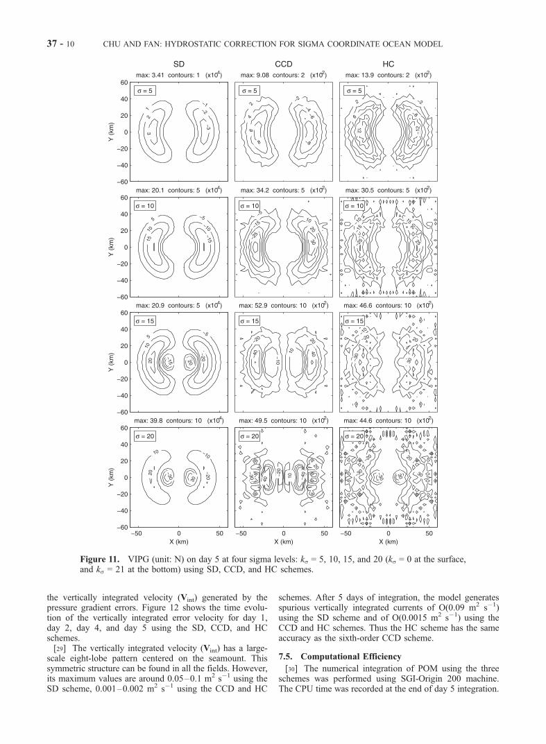
7.3. Volume-Integrated Horizontal Pressure Gradient

[27] The volume-integrated horizontal pressure gradient(@p/@x) for a finite volume (Hdsdxdy) with its center at(x, y, s), denoted by VIPG, is used to represent the sigmacoordinate errors. Figure 11 shows VIPG at day 5 for thesecond-order SD, sixth-order CCD, and HC schemes atfour sigma levels: ks = 5, 10, 15, and 20 (ks = 0 at thesurface, and ks = 21 at the bottom). VIPG reveals adipole pattern at east and west of the seamount at theupper half water column (ks = 5, 10), and a quadrupledipole in the lower layer. VIPG increases with depth fromthe surface (maximum 3.41 � 104 N) to the bottom(maximum 3.98 � 105 N) using the SD scheme). It reducesgreatly using both CCD and HC schemes. Taking ks = 10 asan example, the maximum VIPG is 2.01 � 105 N using theSD scheme, 3.42 � 103 N using the sixth-order CCDscheme, and 3.05 � 103 N using the HC scheme. Thisindicates that the HC scheme has a comparable accuracy asthe sixth-order CCD scheme and reduces the errors by afactor of 70 comparing to the SD scheme.

7.4. Vertically Integrated Velocity

[28] Owing to a very large number of calculationsperformed, we discuss the results exclusively in terms of

Figure 10. Temporally varying MKE (m2 s�2) using SD(dotted), CCD (dashed), and HC (solid) schemes.


the vertically integrated velocity (Vint) generated by thepressure gradient errors. Figure 12 shows the time evolu-tion of the vertically integrated error velocity for day 1,day 2, day 4, and day 5 using the SD, CCD, and HCschemes.[29] The vertically integrated velocity (Vint) has a large-

scale eight-lobe pattern centered on the seamount. Thissymmetric structure can be found in all the fields. However,its maximum values are around 0.05–0.1 m2 s�1 using theSD scheme, 0.001–0.002 m2 s�1 using the CCD and HC

schemes. After 5 days of integration, the model generatesspurious vertically integrated currents of O(0.09 m2 s�1)using the SD scheme and of O(0.0015 m2 s�1) using theCCD and HC schemes. Thus the HC scheme has the sameaccuracy as the sixth-order CCD scheme.

7.5. Computational Efficiency

[30] The numerical integration of POM using the threeschemes was performed using SGI-Origin 200 machine.The CPU time was recorded at the end of day 5 integration.

Figure 11. VIPG (unit: N) on day 5 at four sigma levels: ks = 5, 10, 15, and 20 (ks = 0 at the surface,and ks = 21 at the bottom) using SD, CCD, and HC schemes.


It increases 36% from the SD to CCD, and only 3% fromthe SD to HC scheme (Table 2). No evident CPU increasefrom the SD to HC scheme but the drastic error reductionmake the HC scheme a good choice for the sigma coordi-nate ocean model to reduce the horizontal pressure gradienterror.

8. Comparison Between the Two Test Cases

[31] Comparing to the analytical coastal topography test,the seamount test case yields smaller error reduction. Thelarge difference in the error reduction is caused by theexistence of the two kinds of the sigma error [Mellor et al.,1998]. The two-dimensional coastal topography test only

includes the sigma error of the first kind, which oftendecreases with time. While the three-dimensional seamounttest case also includes the sigma error of the second kindthat depends on the curvature of the topography and doesnot reduce with time. Thus high-order interpolation

Figure 12. Vertically integrated velocity vectors (unit: m2 s�1) at day 1, day 2, day 4, and day 5 usingSD, CCD, and HC schemes.

Table 2. Comparison of CPU Time (Minute) at the End of 5 Day

Runs of the POM Seamount Test Case Using the SD, CCD, and

HC Schemes

Scheme SD CCD HD

CPU Time 171.51 233.33 176.92Ratio 1 1.36 1.03


schemes are especially useful for the second kind of thesigma error.

9. Conclusions

[32] 1. The sigma coordinate pressure gradient errordepends on the choice of difference schemes. By choosingan optimal scheme, we may reduce the error significantlywithout increasing the horizontal resolution. An optimalscheme should satisfy the three requirements: conservation(especially for pressure gradient calculation), high accuracy(especially near the steep topography), and computationalefficiency.[33] 2. The hydrostatic correction scheme has been de-

veloped in this study using the finite volume discretization.The major features of this new scheme are conservation (forpressure gradient calculation), high accuracy, and computa-tional efficiency.[34] 3. Computation of horizontal pressure gradient for

analytical coastal topography with two varying parameters(maximum slope and shelf slope ratio) is used to verify theperformance of the hydrostatic correction scheme againstthe second-order, fourth-order combined, and sixth-ordercombined compact schemes. For all the four schemes, theglobal mean error increases with the maximum slope anddecreases with the shelf slope ratio monotonically. Howev-er, it reduces by a factor of 3.81 from the second-order tofourth-order compact schemes, a factor of 5.00 from thefourth-order compact to sixth-order combined compactschemes, and a factor of 408.8 from the sixth-order com-bined compact to hydrostatic correction schemes. Themaximum error reduces by a factor of 2.39 from thesecond-order to fourth-order compact schemes, a factor of5.96 from the fourth-order compact to sixth-order combinedcompact schemes, and a factor of 32.57 from the sixth-ordercombined compact to hydrostatic correction schemes.[35] 4. For very steep topography, the global mean

pressure gradient error is comparable using any of theexisting schemes (second-order, fourth-order compact,sixth-order combined compact), but 2–3 orders of magni-tude smaller using the hydrostatic correction scheme. Suchhigh performance of the hydrostatic correction scheme isdue to its conservation characteristics for calculating thehorizontal pressure gradient.[36] 5. The standard POM seamount test case is used to

evaluate the performance of the hydrostatic correctionscheme against the second-order, and sixth-order combinedcompact schemes. The hydrostatic correction scheme hascomparable accuracy as the sixth-order combined compactscheme and reduces the errors by a factor of 70 comparingto the second-order scheme. However, its computationalefficiency is comparable to the second-order scheme.

[37] 6. As model resolution increases, the cost for givenaccuracy will eventually favor the high-order methods.While the HC scheme looks the best overall here, morestringent accuracy requirements could be easily satisfiedusing the HC scheme.

[38] Acknowledgments. The Office of Naval Research, the NavalOceanographic Office, and the Naval Postgraduate School supported thisstudy.

ReferencesBlumberg, A., and G. Mellor, A description of a three dimensional coastalocean circulation model, in Three-Dimensional Coastal Ocean Models,Coastal Estuarine Ser., vol. 4, edited by N. S. Heaps, pp. 1–16, AGU,Washington, D. C., 1987.

Chu, P. C., and C. W. Fan, Sixth-order difference scheme for sigma co-ordinate ocean models, J. Phys. Oceanogr., 27, 2064–2071, 1997.

Chu, P. C., and C. W. Fan, A three-point combined compact differencescheme, J. Comput. Phys., 140, 370–399, 1998.

Chu, P. C., and C. Fan, A three-point sixth-order nonuniform combinedcompact difference scheme, J. Comput. Phys., 148, 663–674, 1999.

Chu, P. C., and C. W. Fan, A staggered three-point combined compactdifference scheme, Math. Comput. Model., 32, 323–340, 2000.

Chu, P. C., and C. W. Fan, An accuracy progressive sixth-order finite-difference scheme, J. Atmos. Oceanic Technol., 18, 1245–1257, 2001.

Ezer, T., H. Arango, and A. F. Shchepetkin, Developments in terrain-fol-lowing ocean models: Intercomparisons of numerical aspects, OceanModel., 4, 249–267, 2002.

Gary, J. M., Estimate of truncation error in transformed coordinate primitiveequation atmospheric models, J. Atmos. Sci., 30, 223–233, 1973.

Haney, R. L., On the pressure gradient force over steep topography in sigmacoordinate ocean models, J. Phys. Oceanogr., 21, 610–619, 1991.

Kliem, N., and J. D. Pietrzak, On the pressure gradient error in sigmacoordinate ocean models: A comparison with a laboratory experiment,J. Geophys. Res., 104, 29,781–29,799, 1999.

Lin, S.-J., A finite volume integration method for computing pressure gra-dient force in general vertical coordinates, Q. J. R. Meteorol. Soc., 123,1749–1762, 1997.

McCalpin, J. D., A comparison of second-order and fourth-order pressuregradient algorithms in a sigma-coordinate ocean model, Int. J. Numer.Methods Fluids, 18, 361–383, 1994.

Mellor, G. L., T. Ezer, and L.-Y. Oey, The pressure gradient conundrum ofsigma coordinate ocean models, J. Atmos. Oceanic Technol., 11, 1126–1134, 1994.

Mellor, G. L., L.-Y. Oey, and T. Ezer, Sigma coordinate pressure gradienterrors and the seamount problem, J. Atmos. Oceanic Technol., 15, 1122–1131, 1998.

Shchepetkin, A. F., and J. McWilliams, A method for computing horizontalpressure-gradient force in an oceanic model with a non-aligned verticalcoordinate, J. Geophys. Res., 108(C3), 3090, doi:10.1029/2001JC001047,2002.

Song, Y. T., A general pressure gradient formulation for ocean models. part1: Scheme design and diagnostic analysis, Mon. Weather Rev., 126,3213–3230, 1998.

Song, Y. T., and D. G. Wright, A general pressure gradient formulation forthe ocean models. part 2: Momentum and bottom torque consistency,Mon. Weather Rev., 126, 3213–3230, 1998.

Stelling, G. S., and J. A. T. M. van Kester, On the approximation ofhorizontal gradients in sigma coordinates for bathymetry with steep bot-tom slope, Int. J. Numer. Methods Fluids, 18, 915–935, 1994.

��P. C. Chu and C. Fan, Naval Ocean Analysis and Prediction Laboratory,

Department of Oceanography, Naval Postgraduate School, 833 Dyer Road,Room 328, Monterey, CA 93943, USA. ([email protected])


hydrostatic correction for sigma coordinate ocean models

Documents