Hyper-Local, Directions-Based Ranking of Places

Petros Venetis Hector Gonzalez Christian S. Jensen Alon HalevyStanford University Google Inc. Aarhus University Google Inc.

venetis@cs.stanford.edu hagonzal@google.com csj@cs.au.dk halevy@google.com

ABSTRACTStudies find that at least 20% of web queries have local intent; andthe fraction of queries with local intent that originate from mo-bile properties may be twice as high. The emergence of standard-ized support for location providers in web browsers, as well as ofproviders of accurate locations, enables so-called hyper-local webquerying where the location of a user is accurate at a much finergranularity than with IP-based positioning.

This paper addresses the problem of determining the importanceof points of interest, or places, in local-search results. In doingso, the paper proposes techniques that exploit logged directionsqueries. A query that asks for directions from a location a to a lo-cation b is taken to suggest that a user is interested in traveling to band thus is a vote that location b is interesting. Such user-generateddirections queries are particularly interesting because they are nu-merous and contain precise locations.

Specifically, the paper proposes a framework that takes a user lo-cation and a collection of near-by places as arguments, producinga ranking of the places. The framework enables a range of aspectsof directions queries to be exploited for the ranking of places, in-cluding the frequency with which places have been referred to indirections queries. Next, the paper proposes an algorithm and ac-companying data structures capable of ranking places in responseto hyper-local web queries. Finally, an empirical study with verylarge directions query logs offers insight into the potential of direc-tions queries for the ranking of places and suggests that the pro-posed algorithm is suitable for use in real web search engines.

1. INTRODUCTIONWith the proliferation of high-end mobile devices and improve-

ment to the wireless infrastructure, accessing the Internet from mo-bile phones is becoming commonplace. Current projections arethat in the near future, the sales of high-end mobile devices withcapable browsers will outnumber the sales of desktop computers,and the mobile Internet is slated to become bigger than the con-ventional, wired Internet. Recent studies find that at least 20% ofweb queries have local intent, and the fraction of queries with localintent that originate from mobile properties may be twice as high.

Permission to make digital or hard copies of all or part of this work forpersonal or classroom use is granted without fee provided that copies arenot made or distributed for profit or commercial advantage and that copiesbear this notice and the full citation on the first page. To copy otherwise, torepublish, to post on servers or to redistribute to lists, requires prior specificpermission and/or a fee. Articles from this volume were invited to presenttheir results at The 37th International Conference on Very Large Data Bases,August 29th - September 3rd 2011, Seattle, Washington.Proceedings of the VLDB Endowment, Vol. 4, No. 5Copyright 2011 VLDB Endowment 2150-8097/11/02... $ 10.00.

The emergence of standardized support for location providers inweb browsers, as well as of providers of accurate locations, enablesso-called hyper-local web querying where the location of a user isaccurate at a much finer granularity than with IP-based positioning.

This paper addresses a fundamental problem that arises in mobilesearch: determining the importance of points of interest in local-search results. We consider a setting in which a mobile user queriesthe web for popular near-by places. The user may optionally alsospecify a category of places of interest (e.g., restaurants, attrac-tions, shopping). We assume that a collection of geo-referenced,near-by places is available, but we are agnostic as to how they werecollected (e.g., from a yellow pages service or a web crawl). Thechallenge is to produce a good ranking of the places and to do soin a scalable fashion so that the places can be ranked for any querylocation. While previous work on local-web querying (e.g., [3, 22])assumes IP-based positioning and therefore knows the location ofthe user within a ZIP code, we assume that the user’s location isknown within tens to hundreds of meters, leading to a fundamen-tally different problem.

Our first contribution is to show that logs of directions queriesare a promising source of user-generated content that may enablethe desired ranking. A directions-query log entry contains an ori-gin, a destination, and the time at which the query was issued. Withthe rise in queries to map-based services, such logs are voluminous.In particular, they are much larger and much more current than on-line reviews of points of interest, which would be another sourcefor determining user interest in places. Although one can imag-ine many reasons for issuing directions queries (e.g., to determinemileages for expense reports) a query suggests that there is an inter-est of some kind in the destination. Also, aggregate figures acrosslarge numbers of queries serve to eliminate noise (as confirmed byour studies).

Intuitively, we interpret a query for directions to a point b as avote by a user that point b is of interest. However, we also allowour scoring functions to take several other aspects into considera-tion. First, not all votes are equal: a vote from an origin fartheraway from b could be considered as more important than a votefrom nearby b, as it suggests that the user was willing to travela longer distance to reach b. Second, when candidate places areconsidered in response to a point-of-interest query from a user lo-cation l, the distance to a should be a factor in the ranking. Third,as directions queries have a temporal component, it is relevant toconsider whether temporal patterns in the directions queries can beexploited. For example, users may have different intentions in themorning than in the evening, or on weekdays versus weekend days.

We believe that this is the first research that explores the potentialof directions logs for the ranking of places in local search. Studieshave been reported that aim to identify places that individuals visit

290

from GPS logs and related data sources [7, 17, 18, 19, 25]. Someof these studies also study link-based ranking of places. This pa-per does not consider the identification of places; and it considersranking based on directions queries, not link-based techniques.

Our second contribution is a scalable query processing techniquefor a general hyper-local location-ranking architecture. The archi-tecture, shown in Figure 1, operates in two phases. In the offlinephase, we compute a score for each place in our directory. In theonline phase, we rank places relative to a user’s query location andthe distance the user is willing to travel [16].

Scorer 1

Scorer n

Scorer 2

Hyper−local

Ranking

Retrieval

Top−k places

Query

h−index

...

hcell−rankings

...+

Online

Offline

Places

Figure 1: Architecture for hyper-local ranking

The offline score can combine scores from several scorers, thusleveraging different information sources. In addition to driving di-rections, we can consider the rankings of web pages (or just PageR-ank) associated with places, or reviews that places have received inGoogle or yelp.com. Combining multiple scorers has been con-sidered in previous work [11] and is not considered here.

Our query processing technique superimposes a grid on the space.For each grid cell, called an hCell, we store a list of the places thatfall into the cell, sorted by their (offline) score. At query time, weretrieve the set of hCells relevant to the query and then compute thetop-k places, adjusting the score of each candidate place accordingto its distance to the user’s query location.

We report on experiments that show that real (driving) directionslogs are a viable source for the scoring of places and that the pro-posed framework scales to large data sources and is capable of fastquery response, enabling integration with an existing search engineinfrastructure.

Roadmap: Section 2 presents the problem setting and proposestechniques that use driving directions for place ranking. Section 3then discusses the spatial indexing required to follow our work andpresents a baseline algorithm and a more efficient algorithm forplace ranking. Section 4 considers the suitability of a real driv-ing directions log for ranking of places. Section 5 presents per-formance experiments for the ranking algorithms we propose. Wecover related work in Section 6 and conclude in Section 7. An ap-pendix contains a detailed description of our data sources, someexamples of ranking functions that take into account the directionsquery logs, pseudocode for the baseline algorithm, proofs, and ad-ditional experimental results.

2. RANKING OF PLACES

2.1 Problem SettingA query takes four arguments: (i) the user’s location, (ii) the time

that the query is issued, (iii) the maximum distance the user is will-ing to travel, and (iv) a query string. The query string can be one

of a predefined set of categories, e.g., museums, restaurants, andshopping. This query is capable of supporting a class of popularservices. The result of a query is a ranked list of nearby placesthat match the query string, where the ranking aims to reflect theinterestingness of the places.

To formalize the key concepts of the problem setting, we assumethat a set of places P is given and has signature L × C, where L isthe set of locations in Euclidean space and C is a set of categories(e.g., restaurant, cafe). Places thus model points of interest that auser can visit, and they are categorized. We use Google’s businessdirectory as P .

We also assume that a set D of directions query log entries isgiven, and we use the Google Maps query log. An entry d ∈ D isa record 〈t, a, b, ||a, b||〉 with signature T × L × L× R+. Here, Tis the domain of query times and t is the time when the query wasissued; L was defined earlier, and a is the “from” and b is the “to”of the query; ||a, b|| is the distance between a and b.

A user query q ∈ Q is a quadruple 〈l, t,D, q〉 with signatureL× T ×R+ ×Qq . Here,Qq is the set of all possible strings, i.e.,a set of predetermined categories C, with the empty string denotingall categories. Also, q.D is the distance that the user is willing totravel. This parameter may be specified by the user, or it may bederived from the travel pattern of the user (e.g., walking, driving)using the query logs.

2.2 Scoring FunctionsWe use a scoring function S : Q× P × D to rank an argument

place according to a set of log entries and a user query. Since weuse scoring functions for ranking, the absolute values returned by ascoring function do not matter—only the relative values matter.

Specifically, our framework supports the following kind of scor-ing function:

S(q, p,D) = S(p,D)× weightq.D(||q.l, p.l||).

This function separates the offline scoring from the online scor-ing, as discussed in Section 1. Thus, S(p,D) represents the offlinepart of the scoring, while the weight weightq.D(·) is computed inthe online part. This arrangement enables maximum precomputa-tion for the problem considered. At query time, the offline scoreneeds only be adjusted by a simple multiplication with a score thatdepends on the distance between a query and a place. This is im-portant to achieve low query latency.

We restrict the function weightq.D(·) to be non-increasing, aswe discuss in Section 3.3. This simply means that a user is as-sumed to prefer to travel a shorter rather than a longer distance toachieve the same reward. This assumption also underlies k nearestneighbor querying. Appendix A presents a range of possible scor-ing and weight functions and an experimental comparison of thesefunctions.

2.3 Time-Aware ScoringTime-aware scoring may be applied to any scoring function we

just described. To account for the intuition that users’ behaviorvary across the day and between weekdays and weekend days, weassign different weights to different directions queries according tothe temporal match between their time and the time in the user’squery.

Thus, we can obtain a temporal counterpart of each instance ofthe previous kind of scoring function as follows:

S ′(q, p,D) = S(q, p,D) + α× Stod(q.t)(q, p,D) +

+β × Sdow(q.t)(q, p,D).

291

Here, α and β are positive constants. Function Stod(·) restricts thescoring function to the query log tuples that occur during a particu-lar time of the day. We divide a day into disjoint intervals for morn-ing (06.00–10.00), lunch (10.00–14.00), afternoon (14.00–17.00),dinner (17.00–20.00), evening (20.00–23.00), and night (23.00–06.00). Similarly, function Sdow(·) restricts the scoring functionto the query log tuples that occur during particular sets of days ofthe week: either weekends or weekdays.

We note that the directions query logs can be used in this time-aware setting in contrast to other methods used until now (e.g.,number of reviews, sentiment of reviews).

3. RANKING ALGORITHMSWe assume that a set of places has been retrieved and scored in

an offline phase. We describe two algorithms that then compute thetop-k most relevant places for a query issued by a user at a knownlocation.

We first provide background information on our spatial indexingapproach. Because major search engines (e.g., Google) use space-filling curves to index their geo content, our methods rely on thesetechniques for better integration.

3.1 Spatial IndexingTo efficiently retrieve places located in a given geographic re-

gion, we use a space-filling curve that maps locations on Earth to aone dimensional curve.

5.0.1

5.0.25.0.35.0.0

5.1.05.1.3

5.1.1 5.1.2

5.2.0

5.2.1 5.2.2

5.2.3

5.3.05.3.1

5.3.2

5.3.3 5.0.0.1

5.0.1.1

Figure 2: Example of a Hilbert curve at two levels

We project the Earth’s surface onto the six faces of a unit cube(applying standard transformations to account for distortion). Oneach face of the cube we use the Hilbert curve [21] to map pointsfrom 2-D to 1-D. The Hilbert curve is defined recursively, as exem-plified in Figure 2 that considers part of the 5th face of the Earth.Each cell is subdivided into four smaller cells at each subsequentlevel (identified by the numbers 0, 1, 2, 3 every time). The processstops when the desired granularity has been achieved. We use cellsfrom level 1 (a face in the unit cube) to level 23 (approximately a1 m×1 m cell). We refer to cells in a Hilbert Curve as hCells in thefollowing. Also, we denote as hCellIDl the ID of a hCell at levell. Example hCellIDs can be seen in Figure 2 for l = 3 (left) andl = 4 (right)1. Advise Appendix B for additional details.

Each (latitude, longitude) location is mapped to an hCell at level23. Addresses are mapped into hCells by using a standard geocoder.A geocoder is a piece of software that maps various geographic data(e.g., address, ZIP code) to (latitude, longitude) pairs.

3.2 Table-Based Algorithm (Baseline)We first describe a table-based ranking algorithm. The algo-

rithm uses a table BusinessListing, which contains informa-1We have that hCellID1 ∈ {0, . . . , 5} (face of the Earth) andhCellIDl+1 = hCellIDl.s where s ∈ {0, 1, 2, 3} tells us the or-der by which the Hilbert curve crosses the four smaller squares ofthe hCellIDl.

tion aboutP . The schema of BusinessListing is (PlaceID,Location, Category, Score), where PlaceID is an IDof a place, Location is its location (expressed as an hCell23 iden-tifier), Category is the category to which it belongs (e.g., restau-rant), and Score is the offline score assigned to this place (seeFigure 1), which can be the result of a combination of scores frommultiple scorers.

The table-based algorithm takes as input a subset of the tuples inBusinessListing, namely the places that are within the rangethe user is willing to travel. We use standard spatial indexes tofind such tuples/places. From this subset of tuples, the algorithmcomputes a place ranking by sorting the result tuples according totheir distance-weighted scores (online part of Figure 1). The pseu-docode can be found as Algorithm 2 in Appendix C. The followingexample illustrates the ranking.

EXAMPLE 1. Assume that we have a database with the businessesin Table 1 and that Table 2 contains the information necessary forthe algorithm, computed from the query log.

Table 1: Example business directoryLoc Name Type Category

5.1 . . . Petros’ place Greek restaurant Restaurant5.1 . . . Christian’s place Danish restaurant Restaurant5.0 . . . Hector’s place Colombian restaurant Restaurant5.0 . . . Alon’s place Coffee shop Restaurant5.3 . . . Jack’s place American restaurant Restaurant

Table 2: Statistics of interest for Example 1BusName Offline score Distance (km)

Petros’ place 1000 2.2Christian’s place 700 1.2Hector’s place 200 1.5Alon’s place 500 1.0Jack’s place 550 1.2

We assume that the query q is 〈5.2. . . , 2009/Jun/15 14:23:24.412PST, 2 km, restaurant〉. The relevant set of places then excludesPetros’ place, which is too far away (further than the 2 km that theuser is willing to travel). Assuming a simple linear weighting func-tion (weightq.D(d) = 1 − d/D), the algorithm ranks the resultsas follows: Christian’s place (score = (1−1.2/2.0)×700 = 280),Alon’s place (score = (1 − 1.0/2.0) × 500 = 250), Jack’s place(score = (1 − 1.2/2.0) × 550 = 220), Hector’s place (score =(1− 1.5/2.0)× 300 = 75).

Although this naive algorithm is fast when the set of relevantplaces is small (i.e., the distance the user is willing to travel is smallor the density of places is low), it rapidly degrades as we need toexamine more places. One reason is that the distance function callis expensive.

3.3 Threshold-Based AlgorithmThe algorithm described next adopts the approach of the thresh-

old algorithm [13] and is capable of handling a very large numberof places. This algorithm integrates well with current search en-gines that use space filling curves to index their geo content.

Supported scoring functions. The algorithm accepts any scoringof places that is adjusted with a weighting function weightq.D(d)that decreases monotonically with d, i.e., for di < dj we alwayshave weightq.D(di) ≥ weightq.D(dj).

A simple example in our case would be a scoring function ofthe form: S(p,D) = |{d| d ∈ D ∧ d.b = p.l}|, where d.b is the

292

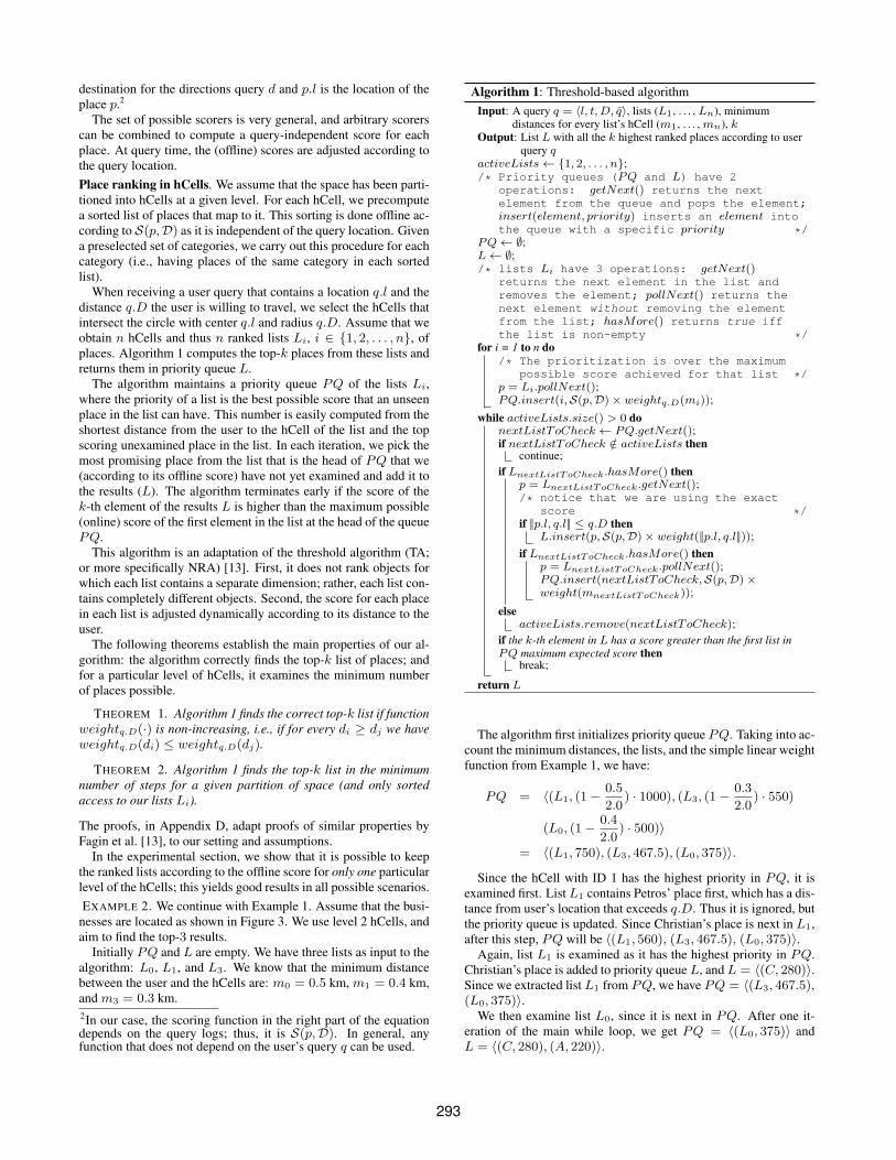
destination for the directions query d and p.l is the location of theplace p.2

The set of possible scorers is very general, and arbitrary scorerscan be combined to compute a query-independent score for eachplace. At query time, the (offline) scores are adjusted according tothe query location.Place ranking in hCells. We assume that the space has been parti-tioned into hCells at a given level. For each hCell, we precomputea sorted list of places that map to it. This sorting is done offline ac-cording to S(p,D) as it is independent of the query location. Givena preselected set of categories, we carry out this procedure for eachcategory (i.e., having places of the same category in each sortedlist).

When receiving a user query that contains a location q.l and thedistance q.D the user is willing to travel, we select the hCells thatintersect the circle with center q.l and radius q.D. Assume that weobtain n hCells and thus n ranked lists Li, i ∈ {1, 2, . . . , n}, ofplaces. Algorithm 1 computes the top-k places from these lists andreturns them in priority queue L.

The algorithm maintains a priority queue PQ of the lists Li,where the priority of a list is the best possible score that an unseenplace in the list can have. This number is easily computed from theshortest distance from the user to the hCell of the list and the topscoring unexamined place in the list. In each iteration, we pick themost promising place from the list that is the head of PQ that we(according to its offline score) have not yet examined and add it tothe results (L). The algorithm terminates early if the score of thek-th element of the results L is higher than the maximum possible(online) score of the first element in the list at the head of the queuePQ.

This algorithm is an adaptation of the threshold algorithm (TA;or more specifically NRA) [13]. First, it does not rank objects forwhich each list contains a separate dimension; rather, each list con-tains completely different objects. Second, the score for each placein each list is adjusted dynamically according to its distance to theuser.

The following theorems establish the main properties of our al-gorithm: the algorithm correctly finds the top-k list of places; andfor a particular level of hCells, it examines the minimum numberof places possible.

THEOREM 1. Algorithm 1 finds the correct top-k list if functionweightq.D(·) is non-increasing, i.e., if for every di ≥ dj we haveweightq.D(di) ≤ weightq.D(dj).

THEOREM 2. Algorithm 1 finds the top-k list in the minimumnumber of steps for a given partition of space (and only sortedaccess to our lists Li).

The proofs, in Appendix D, adapt proofs of similar properties byFagin et al. [13], to our setting and assumptions.

In the experimental section, we show that it is possible to keepthe ranked lists according to the offline score for only one particularlevel of the hCells; this yields good results in all possible scenarios.EXAMPLE 2. We continue with Example 1. Assume that the busi-

nesses are located as shown in Figure 3. We use level 2 hCells, andaim to find the top-3 results.

Initially PQ and L are empty. We have three lists as input to thealgorithm: L0, L1, and L3. We know that the minimum distancebetween the user and the hCells are: m0 = 0.5 km, m1 = 0.4 km,and m3 = 0.3 km.2In our case, the scoring function in the right part of the equationdepends on the query logs; thus, it is S(p,D). In general, anyfunction that does not depend on the user’s query q can be used.

Algorithm 1: Threshold-based algorithmInput: A query q = 〈l, t,D, q〉, lists (L1, . . . , Ln), minimum

distances for every list’s hCell (m1, . . . , mn), kOutput: List L with all the k highest ranked places according to user

query qactiveLists← {1, 2, . . . , n};/* Priority queues (PQ and L) have 2

operations: getNext() returns the nextelement from the queue and pops the element;insert(element, priority) inserts an element intothe queue with a specific priority */

PQ← ∅;L← ∅;/* lists Li have 3 operations: getNext()

returns the next element in the list andremoves the element; pollNext() returns thenext element without removing the elementfrom the list; hasMore() returns true iffthe list is non-empty */

for i = 1 to n do/* The prioritization is over the maximum

possible score achieved for that list */p = Li.pollNext();PQ.insert(i,S(p,D)× weightq.D(mi));

while activeLists.size() > 0 donextListToCheck ← PQ.getNext();if nextListToCheck /∈ activeLists then

continue;if LnextListToCheck.hasMore() then

p = LnextListToCheck.getNext();/* notice that we are using the exact

score */if ||p.l, q.l|| ≤ q.D then

L.insert(p,S(p,D)× weight(||p.l, q.l||));if LnextListToCheck.hasMore() then

p = LnextListToCheck.pollNext();PQ.insert(nextListToCheck,S(p,D)×weight(mnextListToCheck));

elseactiveLists.remove(nextListToCheck);

if the k-th element in L has a score greater than the first list inPQ maximum expected score then

break;

return L

The algorithm first initializes priority queue PQ. Taking into ac-count the minimum distances, the lists, and the simple linear weightfunction from Example 1, we have:

PQ = 〈(L1, (1−0.5

2.0) · 1000), (L3, (1−

0.3

2.0) · 550)

(L0, (1−0.4

2.0) · 500)〉

= 〈(L1, 750), (L3, 467.5), (L0, 375)〉.

Since the hCell with ID 1 has the highest priority in PQ, it isexamined first. List L1 contains Petros’ place first, which has a dis-tance from user’s location that exceeds q.D. Thus it is ignored, butthe priority queue is updated. Since Christian’s place is next in L1,after this step, PQ will be 〈(L1, 560), (L3, 467.5), (L0, 375)〉.

Again, list L1 is examined as it has the highest priority in PQ.Christian’s place is added to priority queue L, and L = 〈(C, 280)〉.Since we extracted list L1 from PQ, we have PQ = 〈(L3, 467.5),(L0, 375)〉.

We then examine list L0, since it is next in PQ. After one it-eration of the main while loop, we get PQ = 〈(L0, 375)〉 andL = 〈(C, 280), (A, 220)〉.

293

L0 = 〈(J, 500), (H, 300)〉

L1 = 〈(P, 1000), (C, 700)〉

L3 = 〈(A, 550)〉0 3

21 0.4 km

0.3 km

0.5 km

P

C

JAH

User

Figure 3: Threshold-based algorithm example

We now examine list L0 since it is next in PQ. After the it-eration, we get L = 〈(C, 280), (J, 250), (A, 220)〉 and PQ =〈(L0, 150)〉. We now have three elements in priority queue L.Since the last element has an actual score that is greater than themaximum possible score of any remaining element in list L0, wehave found the top-3 elements and are done.

4. DIRECTIONS LOGS EVALUATIONWe now describe key characteristics of our data sources (more

details can be found in Appendix E) and show that the directionslog can be a very effective signal for place ranking. Additionalexperiments can be found in Appendix F.

4.1 Key Data Source StatisticsWe use a sample of queries from a travel directions log that con-

tains all the queries issued at Google Maps during July 2009. Wefocus on queries in a sub-region of the United States and thus con-sider the business listings located in this sub-region. We limit theset of business listings to a subset of categories including museums,hotels, restaurants, night clubs, and landmarks.

The query log that we use (D) contains queries for 18,968,123different locations. For the categories of interest we have 151,721business listings (P). It is clear that most of the destinations ofdriving directions queries are not businesses in the directory.

We perform a join between the destination query log and thebusiness directory, on the log destination and the business loca-tion attributes. There are 128,159 businesses for which there is atleast one query with a destination matching the business location.That is, around 84.47% of all business listings in the directory arequeried in the driving directions queries; 0.676% of driving direc-tions queries in D have a business in P as their destination. Al-though, 0.676% is a small percentage, the actual number of queriesissued for the 128,159 businesses is 49,533,223; this number is al-most two orders of magnitude greater than the number of reviewsfor the same places (which was around 550,000). Interestingly,22.5% of the places for which we have directions queries do nothave any reviews, showing that the abundance of directions queriesoffers additional coverage.

In the business directory available, there were multiple busi-nesses located in the same location (hCell23). This happens be-cause the business directory merges several data sources and thenperforms an imperfect Entity Resolution (ER). Furthermore, theinformation extracted from web pages is not always completely ac-curate. The problem of ER in the business listing is orthogonal toour study (see Appendix E.3 for additional details).

Figure 4 shows the distribution of the queries across locationsfor the locations that “survived” the join between D and P , i.e.,locations in which at least one business is located and for which atleast one directions query has the location as its destination. Forexample, in the lower right corner of the figure, we can observethat there is a location that has received ∼8 × 106 queries. In thetop left corner of the figure, we can see that there are around 8,000locations that have received 1 query each.

1

10

100

1000

10000

100

101

102

103

104

105

106

107

Nu

mb

er

of

loca

tio

ns (

log

axis

)

Number of queries (log axis)

Figure 4: Distribution of queries across locations

4.2 Utility of Directions LogsThis experiment investigates the utility of the directions logs sig-

nal. We compare the sets of the top-k results produced and therankings of the results with the corresponding sets and ranking pro-duced by other methods.

We have created a system where a user is able to select a loca-tion the user knows very well and then select a category among thefollowing three: restaurant, point of interest, and hotel. Finally, theuser selects a maximum travel distance. The system then computesthe top-5 places that three methods produce:

1. DL: number of directions log entries that have the place astheir destination,

2. NR: number of reviews for the place under consideration, and3. AR: the average score (sentiment) that reviews have assigned

to the place under consideration.Finally, the resulting 15 places (top-5 from each method) are

shuffled and shown to the user, without the user knowing the ori-gin of each place3. We did not incorporate distance between theuser and a place since we wanted to compare the usefulness of our(offline) signal against two other standard signals. The user is thenasked to evaluate these 15 places with a score between 0 and 4:

Score Specification0 I have no idea of what this is1 Not interesting to most people in general and not recommended2 Neutral to most people in general3 An OK location to most people in general4 Very interesting to most people in general and recommended

Since users are experts in the areas they selected (e.g., around theirhouses or work), their assessments are considered to be of highquality.

We had 10 users select locations, issue queries, and evaluate 15places for each query. A total of 45 queries and 675 places wereevaluated during this process.

We compared the average score that the evaluators assigned tothe top-5 places of each method: our proposed signal (DL) had anaverage score of 1.960, while AR had 1.498, and NR had 1.453.This means that our signal is better at reporting the best places inits top-5 list than the other two signals.

We also evaluated the rankings produced by each method usingthe nDCG metric [15]. This metric can be defined for any list ofevaluated objects; it compares the ranking a method has done (listof objects) to an optimal list of objects according to the evaluationscores. We evaluated nDCG for the top-5 places of each of themethods we examined. The metric takes values between 0 and 1: 1means that the ranking is as expected according to the evaluations,3If there are duplicates among the top-5 lists, we continue deeperinto the lists so that we always show 15 places.

294

and 0 means that the ranking is very bad. DL had nDCG equal to0.787, AR had 0.845, and NR had 0.827.

This study shows that driving directions logs can serve as a strongsignal, on par with reviews, for place ranking. This is an importantfinding because log data offer a number of advantages over reviews,as mentioned in Section 4.3. The fact that the directions-based sig-nal is comparable to the review-based signals is surprising. It is upto a scorer that takes into account multiple signals to decide howthe signals should be combined based on their characteristics.

4.3 Correlation with Number of ReviewsIn this experiment, we evaluate the feasibility of using driving

directions logs as a proxy for the popularity/importance of a place.We compare the correlation of the driving directions based signalwith the number of reviews for a place, which is a commonly ac-cepted measure of popularity. The number of reviews was extractedvia Google’s business directory, and it is the total number of re-views found in various data sources on the Web.

For this experiment, we choose 100 random user locations. Wethen issue the category query “food” and set the distance the useris willing to drive to 2 km. Each of the 100 queries has at least 100ranked results (otherwise, we choose a new random user location).We had to consider 514 distinct places to find 100 user locationswith at least 100 food-related places within a radius of 2 km (∼20%of the randomly selected places had at least 100 results).

We then find the number of reviews of each ranked place forall the queries. We partition the ranked results into batches of tenresults (the top-10, the top-11–20, etc.). For each batch, we sum thenumber of reviews for the places ranked in those places for the 100rankings that we have; the result can be seen in Figure 5. Thereis a clear correlation between the rankings of the results and thenumber of reviews that a place has, which shows that the directionslogs are indicative of the popularity of a place.

These findings are important because driving directions logs arecheap to collect and are orders of magnitude more frequent thanuser reviews, which are expensive to obtain. Further, the logs pro-vide near real-time evidence of changing sentiment, an aspect thatis usually hard to capture with other signals (e.g., the reviews thata place has received; even a newly added web page of a restaurantwill need time to increase its PageRank), and they are available forbroader types of locations.

The scoring function we used for this experiment is S(p,D) =|{d = 〈t, a, p.l, ||a, p.l||〉| d ∈ D}| and weightq.D(d) = 1− d

q.D.

However, similar results are obtained when using other scoring andweighting functions (like the ones described in Appendix A).

5. PERFORMANCE EVALUATIONWe now proceed to report on the evaluation of the runtime per-

formance of the proposed table-based and threshold-based rankingalgorithms in the presence of very large log and place databases.

In the experiments, we assume that the user issues an emptyquery string (retrieve all possible places around me) in order tohave more results to rank. Also, the user is located in a region withhigh business density.

We use the same datasets as described in Section 4.1, and we runall the experiments on a single machine with two AMD dual-coreOpteron CPUs (we only use one of the cores) at 2.2 GHz and with8 GB of RAM.

For the table-based algorithm, we use MySQL as the DBMS withindexing for efficiently determining the places near a user. For thethreshold-based algorithm, we load the ranked lists from the offlinecomputation into memory.

2000

4000

6000

8000

10000

12000

14000

16000

18000

20000

0 10 20 30 40 50 60 70 80 90 100

Nu

mb

er

of

revie

ws f

or

the

ba

tch

Midpoint of the batch

Figure 5: Number of reviews for our ranked list of results

5.1 Table- vs. Threshold-Based AlgorithmFor the threshold-based algorithm we use hCells at level 7 (for

reasons that will be clear later on) and compute the top-100,000results.

Figure 6 presents the ranking time vs. the distance that the user iswilling to travel. It can be observed that the table-based algorithm

1

10

100

1000

10000

1 10 100 1000

Ela

psed tim

e (

msecs)

Distance (kms)

BaselineThreshold method

Figure 6: Performance comparison for our two algorithms

(baseline) takes up to 9.5 secs for large distances (which translatesinto a lot of places), while the threshold-based (efficient) algorithmtakes around 350 msecs in the worst case.

5.2 Varying the hCell LevelIn this experiment, we vary the hCell level from 3 to 23. We

start at 3 because the areas the query logs cover are at this level.We measure the time required to find the top-1,000 results. Themeasurements can be seen in Figure 7 for varying distances (q.D)that the user is willing to travel and for all hCell levels.

0

100

200

300

400

500

600

700

800

0 5 10 15 20 25

Ela

psed tim

e (

msecs)

hCell Level

q.D = 1 kms

q.D = 2 kms

q.D = 4 kms

q.D = 8 kms

q.D = 16 kms

q.D = 32 kms

q.D = 64 kms

q.D = 128 kms

q.D = 256 kms

q.D = 512 kms

Figure 7: Elapsed time vs. hCell level

We observe that the higher the hCell level (i.e., the smaller ourhCells are), the more time is required for our computation for all

295

distances d. This is so because we have to handle more rankedlists of results, which makes the handling of the priority queue PQslower.

We also see that for small distances (like q.D = 1 km andq.D = 2 km), the elapsed time for ranking increases significantlyif one uses a very low hCell level. This happens because we haveto process large lists in order to find results that belong to the smallregion of interest to the user. Put differently, we have to considerplaces that lie in relatively large regions, and that will eventually befiltered given the user’s low willingness to travel.

It seems that a very good trade-off for all possible distances is touse hCell levels 6 or 7. Thus, a search engine can keep statistics foronly one of these two hCell levels and not for every possible level,thus achieving important savings in storage and computation.

5.3 Varying the Value of kNext, we evaluate the time required to find the top-k places for a

fixed maximum travel distance and different values of k. We chosethe distance q.D = 512 km, for a user located in a region with highbusiness density. This setting maximizes the number of places torank, thus imposing a greater burden on the ranking algorithm. Weexperiment with hCell level 7, since the previous experiment showsthat the threshold-based algorithm performs very well at this level.

Figure 8 presents the time required to compute the top-k listsfor several values of k. As expected, the total time increases withk. We note that the process is incremental, meaning that we canfirst find the top-10 results and then, using the same data structures,continue running the algorithm up to the desired level of k.

0

200

400

600

800

1000

1200

0 5 10 15 20 25

Ela

pse

d t

ime

(m

se

cs)

hCell Level

k = 10

k = 100

k = 1000

k = 10000

k = 100000

Figure 8: Time required to find the top-k results for varyingvalues for k

5.4 Performance of Offline ProceduresFor this experiment, we measure the storage and time require-

ments of the offline part of our two algorithms. The MySQL tableBusinessListing is around 89 MB for the table-based algo-rithm (it contains some metadata about the places); the total mem-ory required for the creation of all the ranked lists (based on theoffline score) is around 100.7 MB for all possible levels we haveconsidered.

Both algorithms need to compute the offline score; the additionalcost that the threshold-based algorithm imposes is that one mustcreate ranked lists for each hCell beforehand, which is not requiredin the table-based algorithm. This additional cost (when everythingrun on one machine) is around 25–26 secs for hCell levels 3–8 andthen steadily increases to 28.3 secs for level 9, 31.7 secs for level10, 38.8 secs for level 11, . . . , 329.5 secs for level 23.

We can see that for low levels, the additional offline time is in-significant; as the level of detail increases, the overhead also in-creases. However, the cost is not prohibitive for our method, es-

pecially when we are at levels 6 and 7 where, as we saw earlier,we achieve the best performance. Also, this computation is doneoffline and its cost will be amortized across millions of queries.

6. RELATED WORKFinding interesting locations and/or destinations: A number ofstudies have aimed to identify important locations using primarilyGPS data. Our setting assumes that we know the important lo-cations and that they are classified (e.g., restaurants, hotels); thisinformation is found in business directories.

In the location identification setting, several studies aim to iden-tify places visited by individuals from GPS logs. Ashbrook andStarner [1, 2] present techniques capable of learning significantuser locations and predicting user movement based on GPS data.Brilingaite et al. [4, 5, 6] capture routes and (start and end) destina-tions from GPS trajectories and use these along with temporal us-age information for predicting the routes and destinations of users.Experiments with data from users demonstrate that the techniquesare effective. Krumm and Horvitz [17, 18] also propose techniquesfor destination prediction based on GPS data.

Liu et al. [19] and Cao et al. [7] extract so-called stay pointsfrom the trajectories of users; they propose clustering and reversegeocoding techniques that aim to derive semantically meaningfullocations from the stay points. Zheng and Xie [25] also identifystays from GPS logs, propose a hierarchical containment orderingfor the geographical extents of stays, and then mine so-called lifepatterns of individuals from the resulting location histories. Alongthe same lines Zheng et al. [25], mine locations from GPS trajecto-ries. Here, focus is on identifying public locations, which are thenranked using link-based techniques. Cao et al. [7] offer improvedlink-based ranking techniques.

Our approach can use the results from this line of research asanother source of places (instead of a business directory). Ourapproach does not use GPS data and link-based techniques for itsranking, but considers a different alternative: that of using drivingdirections ranking. GPS datasets typically contain many positionsfor few users; in contrast, directions queries are derived from largeruser populations, with each user issuing few queries.

Ranking functions in a Spatial Context: Other related work dealswith the problem of place ranking [24], where the ranking of ob-jects (e.g., houses) is defined with respect to other qualities aroundthem (e.g., restaurants, schools, hospitals) within a distance range.Also, a framework for the efficient computations of this ranking isprovided. These methods do not try to determine the inherent valueof a place; they determine the value of a place given the fact thatother places are around it. Thus, one could apply our algorithmsand then, as a next step, the algorithms described in [24].

In a more general context, substantial research has consideredlocal search where the results that a user sees for a query dependon the user’s location; the results though are documents and notranked places/businesses (for example, one result could be a blogpost about a particular restaurant), which makes the setting verydifferent. Two recent works in this field propose indexes that areevaluated in terms of efficiently in their settings [8, 26].

In other work [10], NLP techniques are used for geo-searches onthe web. The idea is to find phrases like “next to Eiffel tower” ina hotel’s web document and to thus be able to answer queries like“hotel in Paris” more accurately. Again the output is ranked docu-ments, not ranked places. Our work differs from other techniquesin that no geocoding is used, but only NLP techniques. Means ofdetecting and extracting geographical information (e.g., addresses)from web documents has also been studied [20]. The idea is to

296

extract addresses, phones, ZIP codes and other useful geographicalinformation from a web document and then to augment the locationinformation with keywords from the content of the web document.Query log analysis: Backstrom et al. [3] aim to determine the re-gion of importance for a query, using a probabilistic model. Thiswork does not use positioning, but rather depends on IP-based (10×10 km2) positioning. We try to determine good places, which is dif-ferent from trying to determine the region to which a query is rele-vant. Other work [22] in this line of research aims to determine theso-called dominant location for each query (the location most im-portant for a particular query). The techniques used include querytokenization, query log analysis, and exploration of the snippets ofsearch results for the top-k results.

Work on mobile search log analysis [9] aims to determine howusers search using mobile devices. Some of the explored user be-haviors are the number of keywords in queries, number of queriesper user per day, and search topics.

Finally, there is some work on categorization of queries depend-ing on their scope (local, neighborhood, etc.) [14, 23]. Other workin this area [16] explores the distances that one is willing to travelin order to get to a particular place. This work can be used in ourframework to automatically find a maximum threshold for traveldistance for a given query.TA/NRA comparison: The threshold-based algorithm proposedin Section 3.3 is an adaptation of the threshold algorithm (TA) andmore specifically, a variation of TA called “no random accesses”(NRA) [13]. Both TA and NRA rank objects. Each object has mscores for m different attributes. The overall score of an objectis determined by a combination of the scores for the m attributes,using some monotone aggregation function. For each of the m at-tributes there is a ranked list of the objects according to their scorefor that attribute. TA and NRA find the top-k objects according tothe overall score. TA and NRA differ in that NRA assumes sortedaccess to the ranked lists, i.e., to see the object in the lth positionof a sorted list, one must have seen all l − 1 objects before it. Ouralgorithm differs from NRA in that each list contains different ob-jects in our setting, not a ranking of the same objects for a differentattribute. In addition, in our setting, the score for each place ineach list is adjusted dynamically according to its distance to theuser, which we believe has not been explored in any other work.

7. CONCLUSIONS AND DIRECTIONSGiven the ability to accurately determine the location of a mo-

bile user and the obvious revenue possibilities involved, it is likelythat answering hyper-local queries will receive increasing atten-tion. Our first contribution is to present a new signal, directionslogs, that can be used for scoring places in response to hyper-localqueries. We present key statistics about these logs and show that di-rection queries have a good correlation with the number of reviewsfor places. But unlike reviews and ratings, they are inexpensive tocollect and readily available.

We present an architecture for answering hyper-local queries thatis the first to take into account the distance between a user and aplace and to adjust the score of the place accordingly. To supportthis framework, we propose a threshold-based algorithm that scalesvery well with the number of places under consideration. This algo-rithm returns exact rankings under assumptions that are reasonablein practice.

In terms of future research, we see interesting issues in explor-ing additional scoring functions and methods for combining thesefunctions. In particular, some scoring functions may be more ap-propriate than others for specific types of user queries. Another

interesting aspect of our work is the personalization of the rankingdepending on a user’s specific search history.

Acknowledgments. Christian S. Jensen is an Adjunct Professorat University of Agder, Norway.

8. REFERENCES[1] D. Ashbrook and T. Starner. Learning Significant Locations and

Predicting User Movement with GPS. In ISWC, pp. 101–108, 2002.[2] D. Ashbrook and T. Starner. Using GPS to Learn Significant

Locations and Predict Movement across Multiple Users. Personaland Ubiquitous Computing, 7(5):275–286, 2003.

[3] L. Backstrom, J. M. Kleinberg, R. Kumar, and J. Novak. SpatialVariation in Search Engine Queries. In WWW, pp. 357–366, 2008.

[4] A. Brilingaite. Location-Related Context in Mobile Services. PhDthesis, Aalborg University, 2006.

[5] A. Brilingaite and C. S. Jensen. Enabling Routes of Road NetworkConstrained Movements as Mobile Service Context. GeoInformatica,11(1):55–102, 2007.

[6] A. Brilingaite, C. S. Jensen, and N. Zokaite. Enabling Routes asContext in Mobile Services. In GIS, pp. 127–136, 2004.

[7] X. Cao, G. Cong, and C. S. Jensen. Mining Significant SemanticLocations from GPS Data. PVLDB, 3(1):1009–1020, 2010.

[8] Y.-Y. Chen, T. Suel, and A. Markowetz. Efficient Query Processingin Geographic Web Search Engines. In SIGMOD, pp. 277–288, 2006.

[9] K. Church, B. Smyth, K. Bradley, and P. Cotter. A Large Scale Studyof European Mobile Search Behaviour. In MobileHCI, pp. 13–22,2008.

[10] T. M. Delboni, K. A. V. Borges, and A. H. F. Laender. GeographicWeb Search Based on Positioning Expressions. In GIR, pp. 61–64,2005.

[11] C. Dwork, R. Kumar, M. Naor, and D. Sivakumar. Rank AggregationMethods for the Web. In WWW, pp. 613–622, 2001.

[12] R. Fagin, R. Kumar, and D. Sivakumar. Comparing Top k Lists.SIAM J. Discrete Math., 17(1):134–160, 2003.

[13] R. Fagin, A. Lotem, and M. Naor. Optimal Aggregation Algorithmsfor Middleware. J. Comput. Syst. Sci., 66(4):614–656, 2003.

[14] L. Gravano, V. Hatzivassiloglou, and R. Lichtenstein. CategorizingWeb Queries according to Geographical Locality. In CIKM,pp. 325–333, 2003.

[15] K. Jarvelin and J. Kekalainen. Cumulated Gain-Based Evaluation ofIR Techniques. ACM Trans. Inf. Syst., 20(4):422–446, 2002.

[16] R. Jones, W. V. Zhang, B. Rey, P. Jhala, and E. Stipp. GeographicIntention and Modification in Web Search. Int. J. Geogr. Inf. Sci.,22(3):229–246, 2008.

[17] J. Krumm and E. Horvitz. Predestination: Inferring Destinationsfrom Partial Trajectories. In Ubicomp, pp. 243–260, 2006.

[18] J. Krumm and E. Horvitz. Predestination: Where Do You Want to GoToday? IEEE Computer, 40(4):105–107, 2007.

[19] J. Liu, O. Wolfson, and H. Yin. Extracting Semantic Location fromOutdoor Positioning Systems. In MDM, pp. 73, 2006.

[20] Y. Morimoto, M. Aono, M. E. Houle, and K. S. McCurley. ExtractingSpatial Knowledge from the Web. In SAINT, pp. 326–333, 2003.

[21] H. Sagan. Space-Filling Curves. Springer-Verlag,Berlin/Heidelberg/New York, 1994.

[22] L. Wang, C. Wang, X. Xie, J. Forman, Y. Lu, W.-Y. Ma, and Y. Li.Detecting Dominant Locations from Search Queries. In SIGIR,pp. 424–431, 2005.

[23] X. Yi, H. Raghavan, and C. Leggetter. Discovering Users’ SpecificGeo Intention in Web Search. In WWW, pp. 481–490, 2009.

[24] M. L. Yiu, X. Dai, N. Mamoulis, and M. Vaitis. Top-k SpatialPreference Queries. In ICDE, pp. 1076–1085, 2007.

[25] Y. Zheng, L. Zhang, X. Xie, and W.-Y. Ma. Mining InterestingLocations and Travel Sequences from GPS Trajectories. In WWW,pp. 791–800, 2009.

[26] Y. Zhou, X. Xie, C. Wang, Y. Gong, and W.-Y. Ma. Hybrid indexstructures for location-based web search. In CIKM, pp. 155–162,2005.

297

APPENDIXA. ADDITIONAL SCORING AND WEIGHT

FUNCTIONSWe present some specific examples of possible scoring functions

that can be used in practice. We recall that a place p = 〈l, c〉 has asignature L× C, where L is the set of locations in Euclidean spaceand C is a set of categories that could be of interest to the users.

A.1 Scoring FunctionsCount-based Scoring: The simplest scoring function assigns ascore to a place p that is equal to the count of directions to p:

SC(p,D) = |{d = 〈t, a, p.l, ||a, p.l||〉| d ∈ D}|.

The intuition is that the importance of a place increases with thenumber of users that are willing to travel to reach the place.

Distance-Aware Scoring: With distance-aware scoring, we weighthe contribution to a count by a directions query 〈t, a, b,D〉 by||a, b||, and do not just use a plain count:

SD(p,D) =∑

〈t,a,p.l,‖a,p.l‖〉∈D

||a, p.l||.

The intuition is that the importance of a place increases with thedistance that users are willing to travel to reach the place. If a useris willing to travel long distances, the place is more important thanif the user is willing to travel only short distances to reach it.

Locality-Aware Scoring: With locality-aware scoring, we onlytake into account queries with a distance ||a, b|| similar to the onethe user is willing to travel:

SL(p,D) = |{〈t, a, p.l, ||a, p.l||〉 ∈ D| ||a, p.l|| ≈ ||q.l, p.l||}|.

The intuition behind this scoring function is that people who arewilling to drive similar distances, will more probably want to go tosimilar places.

A.2 Weighting FunctionsLinear Weight: We used two linear weight functions:

weightq.D (||q.l, p.l||) = 1− ||q.l, p.l||q.D

and

weightq.D (||q.l, p.l||) = 1− ||q.l, p.l||2× q.D .

The first one takes the value 1 for ||q.l, p.l|| = 0 and decreaseslinearly to the value 0 for ||q.l, p.l|| = q.D. The second one takesagain the value 1 for ||q.l, p.l|| = 0 and decreases linearly to thevalue 1

2for ||q.l, p.l|| = q.D.

Parabolic Weight: We used two parabolic weight functions:

weightq.D (||q.l, p.l||) = 1− ||q.l, p.l||2

q.D2

and

weightq.D (||q.l, p.l||) = 1− ||q.l, p.l||2

2× q.D2.

The first one takes the value 1 for ||q.l, p.l|| = 0 and decreasesparabolically to the value 0 for ||q.l, p.l|| = q.D. The second onetakes again the value 1 for ||q.l, p.l|| = 0 and decreases paraboli-cally to the value 1

2for ||q.l, p.l|| = q.D.

A.3 Experimental StudyTo study the differences of the various scoring and weighting

functions, we randomly chose 1,000 query locations and ranked allpoints of interest, within a radius of 5 kms with all combinations ofthe scoring and weight functions we defined in Appendix A.1 andA.2.

We used three metrics to compare the ranking produced by dif-ferent scoring functions [12]:Kendall’s Tau: This metric counts the number of times that a pairof entries (α, β) appears in reverse order in the two rankings, i.e.,(α, . . . , β) in ranking one, and (β, . . . , α) in ranking two, normal-ized by the total number of possible pairs.Spearman’s Footrule: This metric counts is defined as the sum ofthe absolute differences between the ranks of an item in two lists(e.g., if place p is 1st in list 1 and 4th in list 2, place p contributes|1 − 4| = 3 to the total sum. We normalize it by dividing by themaximum possible value this sum can have [12].Intersection Metric: When comparing two top-k lists, this met-ric gives the sum of the sizes of the symmetric differences of thetwo lists when considering the top-1, top-2, . . . , top-k elements ofthe two lists, normalized by the maximum possible value of thissum [12].

For all three metrics a value close to 0 signals similar rankings,while a value close to 1 signals different rankings. Using as aweight function a constant function (e.g., weightq.D(||q.l, p.l||) =1), the comparison for the (offline) scoring functions gave the re-sults contained in Table 3, where the Spearman’s footrule for thetop-10 lists is contained (C.-b. stands for Counts-based, D.-a. forDistance-aware, and L.-a. for Locality-aware). Very similar results

Table 3: Comparison of offline scoring functionsCount-based Distance-aware Locality-aware

C.-b. 0 0.430 0.064D.-a. 0.430 0 0.470L.-a. 0.064 0.470 0

were obtained for Kendall’s tau and the intersection metric, andalso for other values of top-k.

Similarly, for the count-based scoring functions we defined inSection A.1, Kendall’s tau metric for the top-20 lists is given inTable 4 (where L.-1 stands for Linear-1, L.- 1

2for Linear- 1

2, P.-1 for

Parabolic 1 and P.- 12

for Parabolic- 12

).

Table 4: Comparison of weight functionsLinear-1 Linear- 1

2Parabolic-1 Parabolic- 1

2

L.-1 0 0.044 0.001 0.060L.- 1

20.044 0 0.048 0.006

P.-1 0.001 0.048 0 0.064P.- 1

20.060 0.006 0.064 0

Very similar results were obtained for Spearman’s footrule andthe intersection metric, other values of top-k and other offline scor-ing functions.

We observe that the actual definitions of the offline scoring func-tions may give substantially different results (look for example thecomparison between the Count-based and the Distance-aware func-tions). Furthermore, the weight functions can also change the rankedlists by a fair amount. While we do not explore with user studieshow to select the appropriate functions, the space is very large andmany different aspects of ranking can be captured in our setting.

298

B. SPACE PARTITIONINGThe following example shows how a (latitude, longitude) pair is

mapped to an hCell’s ID for any possible hCell level.EXAMPLE 3. We denote the hCell ID at level j, where j ∈ {1, 2,. . . , 23}, by hCellIDj . Assume that we are given a location withcoordinates (37.2o,−119.34o), as seen in Figure 9. We want tofind the hCell ID of these coordinates at all levels. In this example,we restrict ourselves to levels 1 and 2.

latitude = 37.2o

longitude = −119.34o

0

1 2

3

hCellID2 = hCellID1.1 = 5.1hCellID1 = 5

Figure 9: Example of hCells

The process is recursive. We first find the hCell ID at level 1 ofthese coordinates; this ID is a number between 0 and 5 (since atlevel 1, we have a cube with six faces). We assume hCellID1 = 5.We then take the rectangle and use the Hilbert curve to number itsfour smaller rectangles. Then, the hCell ID for level 2 becomeshCellID2 = hCellID1.1 = 5.1, as can be seen in the figure.

C. PSEUDOCODE FOR THE TABLE-BASEDALGORITHM

Algorithm 2 contains the pseudocode the straightforward table-based algorithm.

Algorithm 2: Table-based algorithmInput: A query q = 〈l, t,D, q〉, a set of relevant places RP ⊆

BusinessListingOutput: A ranked list of the places in ResultResult←SELECT PlaceID, Score ×weightq.D(||q.l,RP||) AS sFROM RPWHERE RP.Category = qORDER BY s;

The algorithm assumes that all places have been scored and thatthe retrieval module has selected a subset of relevant places, e.g.,places within 10 km of the user’s location. The SQL query simplyreturns the places sorted by their distance-adjusted scores.

D. THEOREM PROOFSHere is the proof of Theorem 1:

Proof: At each point of our algorithm, priority queue PQ containsall the active lists. These are ordered by the maximum possiblescore that a list can contain after removal of the elements we haveseen so far from the list.

The priority queueL contains a ranked list of places that we haveseen in the lists. The ranking for L is over the score S(q, p,D).

The algorithm may stop for two reasons:1. There are no more elements to see in the listsLi: Then priority

queue L contains all the elements ranked by their actual score, andwe have solved the problem correctly.

2. The kth element in L has a score greater than the first listin PQ. Assume the score of the kth -th element in L has score skand the first list in PQ has a maximum possible score sl. Since thealgorithm stopped, we have sk ≥ sl. All the places that have beenexamined so far (and have been included in L) have been rankedaccording to their actual score. Also, all the places that have notbeen examined in the lists have a score that is at most sl ≤ sk.Thus, we know that apart from the current top-k places in L, thereis no other place that can have a score that places it higher than thekth place in L. Thus, we have computed the top-k places.

We need the non-increasing property of function weight(·) toensure that PQ always overestimates the maximum score for thenext element in the list.

Here is a sketch of the proof for Theorem 2:

Proof: Assume we have the ranked lists Li, for i = 1, 2, . . . , nto which we only allow sorted access; sorted access means thatwe have to retrieve elements from the top of each list Li beforeretrieving elements below. Also, assume that the minimum distancebetween the user and the hCell that list Li represents is mi.

Let’s assume that the ranked (by its offline score) content of listLi is 〈pi,1, pi,2, . . . , pi,|Li|〉, for all i. Now assume that we decaythe places in lists Li in order to create the conceptual lists L′i =〈p′i,1, p′i,2, . . . , p′i,|Li|〉; the score of place p′i,j is weightq.D(mi)times less than the score of pi,j . Note that the relative order ofplaces in each list does not change due to the conceptual decayprocess; all places are decayed by the same factor if they are in thesame list.

Each place’s p′i,j offline score has an “error” from its onlinescore that is bounded by a function that takes into account theweight(·) function, the diameter of the hCell and the exact user’slocation. Our algorithm keeps a threshold (let’s call it Ton for thisproof) which is the maximum kth online score seen so far in placesof lists Li (and L′i). At each step, we pick the top place p in listsL′i which has maximum possible offline score soff . If soff < Ton

and we have k examined elements, then we have found the correcttop-k elements.

Now assume that the number of places our algorithm has to ex-amine before it finds the correct top-k places is d. Assume thatthere is another algorithm A that correctly finds the top-k placesin our setting with at most d − 1 steps. Obviously, algorithms Adoes not examine at least one place that our algorithms examines.Let’s call this place p. Say that at that point that algorithm A stopsthe threshold for our algorithm was T ′on. Then, since our algorithmdid not stop at that point and some of the lists L′i had at least theplace p, it was the case that s′off ≥ T ′on. Thus, if p actually had anonline score T ′on (which is possible when place p lies on the pointwith minimum distance from the user’s location and the hCell ofthe list where p is located), then algorithm A would miss a placethat should have been included in the output top-k places.

E. DATA SOURCESWe describe the two main data sources used for place scoring:

the business directory data and the driving directions logs.

E.1 Business DirectoryThe business directory stores information regarding businesses

and their location. An important consideration is high coverage,which is achieved by combining various data sources.

After the business listings have been retrieved, an extensive at-tempt to do Entity Resolution (ER) takes place. A particular restau-rant may have one entry in yelp.com, one in yellowbook.

299

1

10

100

1000

10000

100000

0 50 100 150 200 250Num

ber

of lo

cations (

logarith

mic

axis

)

Collisions

Figure 10: Histogram of collisions

com, one in a blog post, and it may have its own web page. Thisinformation has to be retrieved, cleaned, and then merged into (ide-ally) one entity. Google is very aggressive with respect to ER, inorder to maintain high quality business listings.

After the cleaning and ER, the most accurate address for a busi-ness is geocoded. Thus, we have a very good estimate of the actuallocation of the business (with an accuracy of ∼10 m). Since thegeocoder is the same as the one that was used for the addressesin the direction logs, we can perform a join between the two datasources.

Google’s business directory is a table BusinessListingwithschema (PlaceID, Name, Location, Category), wherePlaceID is an ID for a place, Name is the name of the place,Location is a hCellID23 that captures the location of the place(details on hCellIDs can be found in Section 3.1), and Categoryis one of a few predefined business categories, e.g., museum, restau-rant, university. Table 1 is an example business directory and canbe found in Section 3.2.

Because we have accurate locations of businesses, it is easy todistinguish between two different “branches” of the same chain,e.g., different McDonald’s restaurants.

We derive places from business listings:

Definition 1. We define a place p as a tuple p = 〈l, c, n〉,where l is a location, c is a (business) category, and n is the (busi-ness) name. We may also use the tuple 〈l, c〉 as a place, if the nameof the business under examination is not important.

E.2 Directions LogsThe main data source is the directions logs from Google maps. A

log entry contains a timestamp, an origin (or source), a destination,and the distance from the source to the destination. The followingis an example of a log entry: 〈2009/Jun/15 16:24:43.956PST, 5.2.2.0.3..., 5.2.2.3.2..., 61,043 m〉.

The timestamp is the time when the query was issued and hasan accuracy of 1 ms. The source and destination are given ashCellID23 identifiers. These values are obtained by geocoding thequery strings provided by the user. If a geocode cannot be obtained(e.g., if the source string is not an address but the string “choco-late”), no source value is logged for this attempt to get directions.Thus, we can be certain that if we have valid location IDs then theoriginal query contained actual addresses. The distance betweenthe source and the destination is given in meters and has an accu-racy of some tens of meters.

E.3 Joining the Two Data SourcesWe performed a join between the destination query log and the

business directory, on the log destination and the business locationattributes as we described in Section 4.1.

Let us now examine the number of places that have been as-signed in the same location as other places have been assigned to.

Definition 2. There are k collisions in a particular location li ifthere are exactly (k + 1) places for which p.l = li.

Figure 10 shows the histogram of collisions that appear in thelocations that we have in hand after we perform the join betweenthe query log (D) and the business directory (P).

Most locations contain exactly one place (business listing). Thereare some locations, though, with more than one business. Fromthe empirical evaluation, we have determined that most collisionsoccur because the entity resolution (ER) is not perfect, especiallywhen one has to take into account multiple data sources of busi-ness listings. For example, we have seen examples of two placesin the same location that have the exact same name, or that have aslightly different name (e.g., “La Strada Italian Restaurant” and “LaStrada Ristorante Italiano”), which are the same place, but were notmerged during the ER.

We also note that there are locations with more than 5 businesscollisions. This happens, for example, when the only informationthat we have for a restaurant is the city in which it is located, inwhich case the location of the restaurant is assumed to be the cen-ter of that city. We ignore all the places at locations with 5 ormore collisions in them. We only eliminate 1,733 places with thismethod, which is less than 1.14% of the total business listings inthe region we examine.

The focus of this paper is not on entity resolution, and the busi-ness directory at our disposal is clean enough for place ranking.

F. ADDITIONAL EXPERIMENTALRESULTS

F.1 Directions Log Time DependenceWe study the fluctuations in the number of driving directions

queries for different hours of the day and days of the week. We ex-amined restaurants familiar to us: a steakhouse where people oftengo for dinner on weekdays (it is generally avoided during weekendssince it is slightly isolated), a famous brunch place where peoplego during weekends between the hours of 10 am and 2 pm, and aplace where people gather for drinks and food. Figure 11(a) showsthe normalized number of queries for different hours of the dayfor these three places and for all the restaurants in our business di-rectory. Figure 11(b) shows the normalized number of queries fordifferent days of the week (day 1 is Sunday).

These graphs reveal quite distinct temporal variation. For ex-ample, the brunch place gets the majority of its queries during themornings of the weekends. Similarly, the (isolated) steakhouse re-ceives few queries during the weekends, and the after-work hang-out receives many queries during Friday’s before dinner and lunchtime.

F.2 Directions Logs ContributionIn this experiment we aim to understand whether a place ranking

signal based on driving directions adds new information to an exist-ing place ranking system. The existing place ranking system maytake into account aspects such as the number of reviews, sentimentof reviews, and the PageRank of web pages related to a place. Thepurpose of this experiment is not to quantify the quality of the newsignal, but merely to determine whether it can bring new informa-tion to ranking.

We use Kendall’s tau, described in Appendix A.3, to measurethe distance between two rankings, and we compare place rankings

300

0

0.2

0.4

0.6

0.8

1

1.2

1.4

1.6

1.8

0 5 10 15 20 25

No

rma

lize

d n

um

be

r o

f q

ue

rie

s

Hour of the day

All restaurantsSteakhouse

Brunch placeAfter-work hangout

(a) Hour of the day

0

0.2

0.4

0.6

0.8

1

1.2

1.4

1.6

1.8

0 1 2 3 4 5 6 7 8

No

rma

lize

d n

um

be

r o

f q

ue

rie

s

Day of the week

All restaurantsSteakhouse

Brunch placeAfter-work hangout

(b) Day of the week (day 1 is Sunday)

Figure 11: Normalized number of queries

generated using our scoring function with rankings generated us-ing Google local search (GLS). For our ranking, we use the count-based scoring function (see Appendix A.1) and weightq.D(d) =1− d

q.D.

Figure 12 uses box-whiskers plots to compare top-k rankings fork = 5, 10, 15, . . . , 100 using Kendall’s tau. The boxes contain thevalues between the first quartile and the third quartile. The endpoints represent the minimum and maximum values observed forthe measurements, while the line inside the box is the median. Wesee that the median of new information is around 50% for all thevalues of k considered. Also, it tends to stabilize as k gets larger.

0

0.2

0.4

0.6

0.8

1

0 20 40 60 80 100

Kendall’

s tau

Number of top-k results under comparison(in multiples of 5)

GLS comparison

Figure 12: Count-aware scoring versus GLS ranking

We note that no existing system explicitly uses a weightq.D(·)function for the distance. Usually current systems just rank placesthat are in the user’s ZIP code, irrespectively of the user’s distanceto the places, or they use other heuristics similar to this. Thus, it isexpected that the use of directions logs will add new information toany existing ranking system.

F.3 Sensitivity to the User’s LocationIn this experiment, we examine how sensitive our ranking func-

tions are to the exact location of a user.For examining the sensitivity of our ranking functions to the ex-

act location of a user, we use the simple weightq.D(·) functionweightq.D(d) = 1 − d

q.Dand the count-based scoring function

(see Appendix A.1), which basically just counts the queries for aparticular location.

The settings for the experiment are as follows. We have 100hypothetical users. Each user is located in a randomly chosen lo-

cation, the user issues the query “food” (one of the predeterminedcategories), and the user is willing to travel 2 km. For each one ofthe 100 users, we select 400 locations, such that their distances tothe user are less than ∼1.4 km.

For each one of the 400 locations, we re-rank the results thatwere initially ranked for the associated user’s location, using theranking function S(q′, p,D), where q′ and q are only different inthe user’s location (q.l is the user’s original location and q′.l is oneof the 400 locations around the user). Then we compare the top-klists of the two lists using Kendall’s tau (with parameter p = 0).

0

0.02

0.04

0.06

0.08

0.1

0 200 400 600 800 1000 1200 1400

Kendall’

s tau

Distance from original point (meters)

Location sensitivity

Figure 13: Location sensitivity of our ranking functions

We have included all the comparisons of the top-50 lists for var-ious distances and we present a box-whiskers plot (as described inAppendix F.2) for distances that are less than 100 m, 200 m, . . . ,1,400 m in Figure 13.

One can observe that two ranked lists are very similar (there isa difference that is less than 1%) for distances of around 100 m.The similarity decreases rapidly with distance, to around 8% for adistance of 1.4 km. This provides evidence of the importance ofhyper-local ranking. When the precise location of a user is known,we can do a better job of ranking locally interesting places.

The results for other scoring functions (e.g., the ones describedin Appendix A.1) and different values of k (for the top-k lists) werevery similar. We also experimented with some other weight func-tions (e.g., the ones described in Appendix A.2); again, the resultsare very similar to the ones presented here. Of course, the graphdepends on how fast the weightq.D(·) function decreases, but noqualitative differences were observed during our experiments.

301