The Regional Economics Applications Laboratory (REAL) is a unit of the University of Illinois focusing

on the development and use of analytical models for urban and region economic development. The

purpose of the Discussion Papers is to circulate intermediate and final results of this research among

readers within and outside REAL. The opinions and conclusions expressed in the papers are those of the

authors and do not necessarily represent those of the University of Illinois. All requests and comments

should be directed to Geoffrey J. D. Hewings, Director, Regional Economics Applications Laboratory,

607 South Matthews, Urbana, IL, 61801-3671, phone (217) 333-4740, FAX (217) 244-9339.

Web page: www.real.illinois.edu.

INTER-REGIONAL ENDOGENOUS GROWTH UNDER THE IMPACTS OF DEMOGRAPHIC CHANGES

Tae-Jeong Kim and Geoffrey J.D. Hewings

REAL 10-T-3 April, 2010

- 1 -

Inter-Regional Endogenous Growth under the Impacts of Demographic Changes

Tae-Jeong Kim

Regional Economics Applications Laboratory, University of Illinois at Urbana-Champaign, 607 S.

Mathews, Urbana, IL 61801

tkim35@illinois.edu

Geoffrey J.D. Hewings

Regional Economics Applications Laboratory, University of Illinois at Urbana-Champaign, 607 S.

Mathews, Urbana, IL 61801

hewings@illinois.edu

ABSTRACT: This paper attempts to project the economic paths for the individual

Midwest states (Illinois, Indiana, Michigan, Ohio and Wisconsin, as well as the Rest of

the US) in the near future when the population ageing becomes more pronounced. To

accomplish this task, a dynamic general equilibrium model is developed so that it could

incorporate the inter-regional transactions and endogenous growth mechanisms within

the framework of an overlapping generations (OLG) model. Key parameter values

associated with the regional interconnections were assigned by using multi-regional

Social Accounting Matrix (SAM) of the Midwest states. Two different steady-state

results were presented with two different age-cohort population structures corresponding

to year 2007 and 2030. These steady-state results imply that the rate of declining of per-

capita output are projected to be heterogeneous across the regions due to the different

developments of age-cohort population structures and consequently different levels of

endogenously determined educational investment of workers. Also two steady-state

simulation results revealed that the development of output price in a certain region

reflects the dynamics of demographics of every region. Meanwhile, the dynamic

simulation results reveal that the per-capita output of every region is projected to grow

positively in the near future when the population ageing will be pronouncing. However,

the growth rate of the per-capita output is projected to be heterogeneous across the

regions: the regions with high-skilled workers hold the potential threat that population

ageing could give more negative impacts on the economy due to the relatively sluggish

growth of human capital stock. Also, the dynamic simulation results show that certain

regions in Midwest will experience their terms-of-trade deteriorate in the near future,

implying that careful attention should be given to their future trade conditions.

KEY WORDS: Human Capital; Overlapping Generations; Inter-Regional Transaction;

Demographic Transition; Social Accounting Matrix (SAM); Terms of Trade

- 2 -

I Introduction

This paper attempts to project the economic paths for the individual Midwest states

(Illinois, Indiana, Michigan, Ohio and Wisconsin, as well as the Rest of the US) in the

future when the population ageing becomes more pronounced. To accomplish this task, a

dynamic general equilibrium model is developed so that it could incorporate the inter-

regional transactions and endogenous growth mechanisms within the framework of an

overlapping generations (OLG) model.

There has been expanding literature that has adopted OLG models to explore the

issues of demographic change. In particular, the papers that used the OLG model and the

endogenous growth mechanism showed that the negative impact of population ageing

could be mitigated through the revelation of educational motive on the part of workers

since educational investment in developing workers’ human capital could improve the

overall productivity in the corresponding economy and thus significantly attenuate the

shortage of labor force. The literature includes the work of Sadahiro and Shimasawa

(2002) and Ludwig et al. (2007). Although those two papers accepted different human

capital technology under different scenarios of age-population projection, they found out

that the individual’s educational motive substantially adjusts the effect of population

ageing. However, their papers did not pay attention to the interconnections between the

regions, assuming implicitly that all transactions including exchanging intermediate

inputs and consumption and investment goods are done in single economy. However,

when multiple economies are interconnected with each other, then the different scale of

demographic changes in one region should bring about the different flows of transactions

- 3 -

between the regions. It is important to develop a dynamic model that could recognize the

interconnections between the regions.

Fougere et al. (2004) showed the effect of population ageing in Canada under

some alternative scenarios. In this context, they presented different demographic

scenarios depending on the different number of immigrants and immigration destinations.

The main contribution of this paper is to introduce an inter-regional OLG framework to

capture the interactions of six regions of Canada. For this, they assumed that the regional

goods are imperfect substitutes each other; and each region’s purchase of consumption

and investment goods from the six regions are ruled by a constant elasticity substitution

(CES) function. They assumed no transactions of intermediate goods between the

regions; and the productivity of each age-cohort was exogenously given.

A multi-regional social accounting matrix (SAM) records all the transactions

between the regions in a certain fiscal year. This valuable source could be useful to

calibrating the parameters in the inter-regional model, especially related to the regional

demand function for the goods produced in other regions. There are not many papers that

use a SAM in the process of calibrating a dynamic general equilibrium model. Among

them, Kehoe et al. (1995) and Kehoe (1996) could be regarded as a starting point for

using SAM in general equilibrium models. Kehoe et al. (1995) and Kehoe (1996)

attempted to use social accounting matrices (SAMs) in muti-sectoral general equilibrium

models. Those papers used the transaction data of Spanish (national-level) SAM to

calibrate the parameter in consumption, investment and production function. Adopting

the disaggregated model specification, where 12 production sectors, 9 consumption goods

- 4 -

and 3 factors of production, those papers simulated the Spanish economy and presented

the impacts of Spain’s integration into the European Community.

This paper is organized as follows. In section II, the model description will be

presented. In section III, the calibration procedure will be described, focusing on the

regional production, consumption and investment demand function, by using an

aggregated six-regional Midwest SAM for year 2007 that was compiled by the Regional

Economics Applications Laboratory (REAL) at the University of Illinois at the Urbana-

Champaign (UIUC). In section IV, computational results including steady-state results

and dynamic results will be presented. In the final section, conclusions will be drawn and

suggestions for further research will be briefly discussed.

II Model description

The model represents the US economy through the specification of 6 regions- Illinois

(IL=1), Indiana (IN=2), Michigan (MI=3), Ohio (OH=4), Wisconsin (WI=5) and the rest

of US (ROUS=6). The economy is closed to the rest of the world; thus, there are no

foreign imports or exports in the model. There are two types of economic agents in each

region: a representative firm and households. Each year, there are 65 overlapped

generations in the household sector. Also there is a federal government to operate a

social security system in each region. The economy produces physical goods as well as

human capital. Physical goods are tradable across regions; and the firm can purchase

intermediate goods from each region. Also, consumers and investors purchase goods

from all the regions for consumption and investment purposes respectively.

- 5 -

1 Production

Regional production functions specify intermediate input requirements of both factors,

such as labor and capital, and other regional goods. Following Kehoe (1996), a

requirement of fixed input per unit production is assumed for a composite input of

regional goods as well as for value added. Factor input requirements are represented by

Cobb-Douglas value-added functions. Defining ,j t

Y as the gross output in region j at

period t , the general form of production technology is as follows:

, 1 , 1 6 , 6 , ,min( / ,......, / , / )

j t j t j j t j j t VA jY x z x z VA z= (1)

where ij

z is the amount of intermediate good produced in region i , required to produce

one unit in region j , ,VA j

z is the fixed value-added requirement per unit production in the

region j , ij

x is the intermediate input of regional good produced in region i ; and ,j t

VA is

the value added. Value added technology is assumed to take a Cobb-Douglas form:

1

, , ,

j jd d

j t j j t j tVA A K L

α α−= (2)

while jA is a parameter of total factor productivity (TFP), d

jK is a demand for physical

capital stock, d

jL is a demand for effective labor for the value added and jα is a

parameter of capital income share. We assume that labor is immobile. Since producers

minimize cost, they never waste their inputs. Thus,

1

, 1 , 1 2 , 2 , , ,/ / .... /j jd d

j t j t j j t j j j t j t VA jY x z x z A K L zα α−

= = = = holds.

The firm’s optimization problem is to solve:

Max 6

, , , , , , , , ,

1

d d

j t j t j t j t j t j t j t i t ij t

i

p Y w L rr K p xπ=

= − − −∑ (3)

- 6 -

where rr is a rental return of physical capital belonging to investors, w is a wage rate for

one effective labor unit. This problem leads to the following first order conditions:

,

16

,

, , , ,

1,

j

j t

d

j j j t

j t j t i t i jdiVA j

A Krr p p z

z L

α

α−

=

= −

∑ (4)

6,

, , , ,

1, ,

(1 )jd

j j j t

j t j t i t i jdiVA j j t

A Kw p p z

z L

αα

=

− = −

∑ (5)

where p is output price. These conditions reveal that the marginal product of capital and

labor should be depreciated by the cost of buying intermediate goods which complement

the labor or capital input. That is, the rental return and wage rate is positively correlated

with the terms of trade. If the output price in region j becomes relatively higher than the

other regions, then this relative increase should be reflected by factor prices. Also,

conditions (4) and (5) imply that firms earn zero profit in every region at every period

since the market is assumed to be perfectly competitive.

2 Consumption

In each region at every period, households are represented by 65 overlapping generations.

Each individual is assumed to live 65 periods: each individual is born and enters the labor

market at age 1 (real age 20), works until age 45; and lives until age 65 (real age 84).

A household’s inter-temporal optimization problem consists of choosing a

sequence of consumption and educational investment share over the life-time in order to

maximize life-time utility subject to life-time wealth. The following formulation is a

current period preference of a representative household of generation g in region j at

period t :

- 7 -

1 1

, , , ,

, , , ,( , )

1

j g t j g t

j g t j g t

c eu c e

γ γθ

γ

− −+=

− 1γ > , 0 1θ< < (6)

where c denotes a consumption bundle, which is composed of the final goods produced

in each region; and e is a educational investment share of individual’s time endowment

(=1) with γ determining the inter-temporal elasticity of substitution and θ being a

parameter representing the degree of educational investment motive. Thus, life-time

utility of a representative individual born at time t in the region j is as follows:

1

1, , 1

145 45

, , 11

, , 1 , , 1

1 1

( , )1

gj g t gj g t gg

t j g t g j g t g

g g

c eU u c e

γ γθβ β

γ

−

−+ −

−+ −−

+ − + −= =

+ = = −

∑ ∑ (7)

where β denotes the subjective discount factor.

The individual who was born in the region j at time t has a following life-time budget

constraint:

2 265 45

, , 1 , , 1 , 1 , , 1 , 1 , , 1

1 1, ,

1 1(1 ) (1 )

1 1

t g t gc p

j g t g j g t g j t g j g t g j t g j g t g

g gk t k tj k j k

p c h w er r

τ+ − + −

+ − + − + − + − + − + −= == =

= − − + +

∑ ∑∏ ∏

265

, , 1

46 ,

1

1

t g

j g t g

g k t j k

penr

+ −

+ −= =

+ + ∑ ∏ (8)

where ,j tr denotes the rate of return on capital stock in the region j at time t , , ,

c

j g tp is

consumption price index, ,

p

j tτ is a pension tax on earnings in the region j at time t and

, ,j g th denotes human capital stock of age-cohort g in the region j at the time t . This

budget constraint means that present value of life-time consumption (i.e., left-hand side

of the equation 8) should be exactly the same as the present value of life-time wealth

composed of labor income and pension benefits (i.e., right-hand side of 8). It is assumed

- 8 -

that there is no unexpected death until the age 65; thus there should not be unintended

bequests. Note that the current period budget constraint is as follows:

, 1, 1 , , , , , , , , , , , , ,(1 ) (1 ) (1 )p c

j g t j t j g t j t j t j g t j g t j g t j g ta r a w h e p cτ+ + = + + − − − (if 45g ≤ ),

, 1, 1 , , , , , , , , ,(1 ) c

j g t j t j g t j g t j g t j g ta r a pen p c+ + = + + − (if 46g ≥ ).

(9)

Now, the inter-temporal Euler equations are computed from the household’s

optimization problem (7) subject to (8) as follows:

1/

, 1 , ,

, 1, 1 , ,

, 1, 1

(1 )c

j j t j g t

j g t j g tc

j g t

r pc c

p

γβ +

+ +

+ +

+=

(10)

1/

, ,

, , , ,

, , ,(1 )

c

j g t

j g t j g tp

j t t j g t

pe c

w h

γθ

τ

= −

(if 45g ≤ ) (11)

Then, aggregate consumption demand in the region j at the period t could be

characterized as:

, , , , ,j t j g t j g t

g

C N c=∑ (12)

where , ,j g tN is the number of population belonging to the age-cohort g in the region j at

time t .

In the next optimization step, Armington’s (1969) strategy is applied to allocate

the household’s consumption expenditure across each region’s produced goods.

Consumers are assumed to consider each region’s goods as imperfect substitutes. Given

this assumption, a CES type sub-utility function of households can be developed:

1

1

, , , , , ,( )

cc c jj jc c

j g t i j i j g t

i

c dσσ σ

υ−

= ∑ (13)

- 9 -

where , , ,i j g t

cd denotes the demand for the final good produced at the region i by

individuals of age-cohort g living at the region j ; and ,

c

i jυ is a preference parameter

determining a consumption distribution across regional goods; and c

jσ determines the

elasticity of substitution across regional goods at the region j . Then, by the first order

condition of household’s optimization problem, the demand for region i product by the

region j consumers is specified as follows:

, , ,

1

1,

, , ,

,

cj

i j g t

c

j tc c

i j j g t

i t

pd c

p

σ

υ−

=

(14)

where ,i tp is the output price of goods produced at the region i at the time t . The

consumption price index ( ,

c

j tp ) can be computed as a non-linear weighted average of each

region’s output price:

1 1

, , ,

c cj j

c cj jc c

j t i j i t

i

p p

σ σ

σ συ

− −

− −=∑ (15)

3 Investment

After consumption and social security payments, the rest of an individual’s disposable

income is saved in the form of investment in physical capital for the next period. The

aggregate supply of physical capital at the region j can be defined as follows:

, , , ,

,

,

j g t j g t

gs

j t I

j t

N a

Kp

=∑

(16)

where Ip denotes the unit price of the investment good and sK is a aggregate supply of

physical capital.

- 10 -

The law of motion for the physical capital stock is as follows:

, 1 , ,(1 )s k s

j t j t j tK Inv Kδ+ = + − (17)

where kδ denotes the depreciation rate of physical capital; and ,j tInv represents the

aggregate investment bundle in the region j . Investment activity is supposed to be inter-

regional, implying that the investment bundle in the region j ( ,j tInv ), which was

purchased in region j for the investment purpose, is composed of each region’s produced

good. The investment bundle ( ,j tInv ) is formed as a CES function that combines the

goods from the six different regions as follows:

1

1

, , , ,( )

II I jj jI I

j t i j i j t

i

Inv dσσ σ

υ−

= ∑ (18)

where , ,

I

i j td is the quantity of goods produced in region i , that is demanded by the

investor1 of region j ; ,

I

i jυ is the preference parameter determining a regional distribution

of investment goods and I

jσ determines the elasticity of substitution across the regional

goods. Then, an investor chooses the optimal portfolio of regional goods according to the

following equation:

, ,

1

1,

, ,

,

Ij

i j t

I

j tI I

i j j t

i t

pd Inv

p

σ

υ−

=

(19)

Now, ,

I

j tp can be computed as a non-linear weighted average of each region’s output

price:

1 There is no investor in this model explicitly. However, for the purpose of interpretation of model

specification, an investor could be understood as a group of individuals in each region; and an investor is

supposed to decide the composition of portfolio of the aggregate investment in his/her region.

- 11 -

1 1

, , ,

I Ij j

I Ij jI I

j t i j i t

i

p p

σ σ

σ συ

− −

− −=∑ (20)

The rate of return from investment in physical capital should be composed of

rental return and a capital gain as follows:

, ,

,

, 1

(1 )1

k I

j t j j t

j t I

j t

rr pR

p

δ

−

+ −+ = (21)

where ,j tR denotes the (net) rate of return from the investment in physical capital. There

are no financial assets in this economy, so this rate of return will serve as a bench mark

interest rate; thus , ,1 1j t j tr R+ = + for all j .

4 Social security

The federal government operates a pay-as-you-go (PAYG) style pension system. Under

the PAYG system, the government levies a social security tax ( pτ ) on labor income and

transfers the pension benefit to the retirees. There is neither public debt nor other forms

of taxation from the governments. The pension benefit ( pen ) is assumed to be a fraction

of average life-time labor income and this fraction rate (ξ ) is identical across the regions.

The pension benefit is fixed according to the following:

45

, 46, , , ( ) , ( ) , , ( )

1

(1 )j G t j g t G g j t G g j g t G g

g

pen e w hξ≥ − − − − − −=

= −∑ (22)

The social security tax is endogenously determined so that the federal government’s

pension system is assumed to be balanced every period as follows:

( )45 65

, , , , , , , , , , ,

1 46

(1 )p

t j g t j g t j t j g t j g t j g t

j g j g

N e w h N penτ= =

− =

∑ ∑ ∑ ∑ . (23)

- 12 -

5 Human capital

The human capital technology is governed by the following specification proposed by

Sadahiro and Shimasawa (2002):

1

, 1, 1 , , , , , , ,(1 ) ( ) ( )j g t h j g t j t j g t j g th h B mk h eφ φδ −

+ + = − + (24)

where t

k is the physical capital/labor ratio while B is the parameter for the accumulation

efficiency of human capital, m is the portion of physical capital stock used for producing

the human capital stock, h

δ is the parameter of depreciation rate of human capital stock

and φ is the parameter of the elasticity of human capital formation function.

Human capital is transmitted between generations according the following rule:

45 45

,1, , , 1 , , 1 , , 1

1 1

/hc

j t j g t j g t j g t

g g

h h N Nπ − − −= =

=

∑ ∑ (25)

where hcπ is the parameter of human capital transmission factor. This parameter can be

interpreted as the degree of quality or efficiency to pass the available stock of knowledge

from generation to generation. If a society can provide the individual a successful

educational environment (either formally or in-formally) in childhood and youth so that

the individual earns the cognitive ability and creativeness well in these period, this

parameter value should be high since the human ability acquired early will make post-

secondary learning easier.

The aggregate human capital stock of region j at time t is defined using (26); and

the aggregate supply of labor can be computed using (27):

45

, , , , ,

1

j t j g t j g t

g

H h N=

=∑ (26)

45

, , , , , , ,

1

(1 )s

j t j g t j g t j g t

g

L e h N=

= −∑ (27)

- 13 -

6 Competitive equilibrium

A competitive equilibrium of the economy is defined as a dynamic and spatial sequence

of regional disaggregate variables { , , , , , ,, ,j g t j g t j g tc e a } , ,j g t ; regional aggregate variables

{ , , , , , ,, , , , ,s s d d

j t j t j t j t j t j tC K L K L Inv } ,j t ; regional demand variables { , , ,

c

i j g td } , , ,i j g t and { , ,

i

i j td } , ,i j t ;

regional intermediate demand variable { ,ij tx }, ,i j t

; regional output price and factor prices

{ , , ,, ,j t j t j tp rr w } ,j t ; the interest rate { ,j tr } ,j t ; and the regional pension contribution rate

{ p

tτ }

t where ,i j =IL, IN, MI, OH, WI and ROUS; g is the age-cohort from 1 to 65; and

t denotes year which satisfy 1) through 4):

1) Given prices and interest rate, the allocations are feasible for every region at every

period: , , , , , , , , ,

c I

i t ij t j g t i j g t i j t

j j g j

Y x N d d= + +∑ ∑∑ ∑ , , ,

s d

j t j tL L= and , ,

s d

j t j tK K= .

2) Output prices and factor prices { , , ,, ,j t j t j tp rr w } ,j t satisfy (4) and (5) for every region at

every period; and (21) holds for every period.

3) Given prices and the interest rate, disaggregate variables { , , , , , ,, ,j g t j g t j g tc e a } , ,j g t satisfy

(9), (10) and (11) for every generations for every region at every period.

4) Given prices and interest rate, the pension contribution rate { p

tτ }

t satisfies (23) for

every region at every period.

III Calibration

This section will focus on the estimation of the parameter values in the production,

consumption and investment functions. There are very little data available necessary for

statistically estimating the inter-regional elasticity of substitution in consumption and

- 14 -

investment functions described in the previous section. For example, there are only four

sets (that is, 1993, 1997, 2002 and 2007) of data from the Commodity Flow Survey

(CFS). Also, there are no time-series of SAMs to provide the possibility for estimating

the price elasticities of consumption and investment across the regions. However, there

is some literature that has attempted to estimate the regional import elasticity of

substitution in the US, focused on individual industries. For example, Bilgic et al. (2002)

estimate the elasticity of import substitution for 20 industry groups between 48 states,

based on the micro-level data of 1993 CFS. In this paper, for the regional elasticity of

substitution, this work is used as a benchmark; thereafter, the preference parameters of

consumers and investors in each region from the six-regional Midwest-SAM are

developed. For the human capital technology, the parameter values are assumed to be

identical across regions, drawing on those available for the US economy in Sadahiro and

Shimasawa (2002).

1 Production function

Table 1 is provides the expenditure quantities across regions for all industries in each

state derived from input-output table of the Midwest. Since this paper does not consider

sectors of institutions as well as tax and transfer of government and international trade,

we exclude the products of institution and indirect business taxes as well as exports and

imports in the table when calibrating the parameters. Also it should be noted that the

original values in the IO table are denominated by the consumer price index (CPI) of

each corresponding region (see table 2 for the regional coverage of CPI). Thus, each

number in the cell in the table 1 is a unit-free quantity.

- 15 -

The parameters determining the quantity of intermediate goods across regions

(that is, ij

z ) could be computed as shares of expenditures from the table 1. The capital

and labor income shares are also computed from the same table. Table 3 reveals the

parameter values, which will be assigned to the production function.

2 Consumption and Investment functions

The elasticity of substitution in consumption and investment across regional goods is set

to be 1.103, derived from the result of Bilgic et al. (2002). This number is the estimated

elasticity of import substitution of all commodities. This elasticity is assumed to be

homogeneous across regions and generations. Using this parameter value, the preference

parameter of each region in consumption and investment could be computed with the

information of consumption and investment shares of each region (table 4). Note that the

magnitude in this table is also a unit-free quantity.

From (14), the preference parameter of consumption (,

c

i jυ ) could be computed as

follows:

,

,

cj

i j

sc c

jc

i j

j i

d p

c pυ

−

= ×

(28)

where 1/(1 )c c

j js σ= − is nothing but an elasticity of substitution for consumption; and

1 1

, , ,

c cj j

c cj jc c

j t i j i t

i

p p

σ σ

σ συ

− −

− −=∑ . Also, from (18), the preference parameter of investment (

,

I

i jυ ) can

be estimated as:

,

,

Ij

i j

sI I

jI

i j

j i

d p

Inv pυ

−

= ×

(29)

- 16 -

where 1/(1 )I I

j js σ= − is a elasticity of substitution across regional investment goods; and

1 1

, , ,

I Ij j

I Ij jI I

j t i j i t

i

p p

σ σ

σ συ

− −

− −=∑ . Table 5 shows the calibration results.

IV Computational results

1. Steady-state

In this section, before presenting the results of the dynamic simulation, the steady state

simulation results will be briefly summarized. For this presentation, the age-cohort

population structure is adopted from the Census Bureau’s estimation for the year 2007.

Figure 1 shows the age-cohort structure that was adopted into the model for the steady

state simulation. Note that IL’s total population is normalized to a unit

(65

, , 2007

1

1j IL g t

g

N = ==

=∑ ). Table 6 reveals that OH has the highest dependency ratio; and IL has

the lowest. Figure 1 reveals that IL has significantly more people belonging to the

below-retirement age than OH; but IL has almost same number of people belonging to

the retirement age as OH. This could be interpreted as the result of retirement migration

out of IL2. For the steady state analysis, this age-cohort population structure is assumed

to be maintained in the long-term; also, it is assumed that there will be no change in

prices including output, consumption and investment prices as well as factor prices such

as the rental return and the wage rate. These assumptions described above would not be

2 According to the 2008 American Community Survey (ACS) data, Illinois ranked the 2

nd state after New

York in the volume of losing the elderly residents (age 65+) through the out-migration during the previous

one year.

- 17 -

maintained in the dynamic simulation, the results of which will be presented in the next

section.

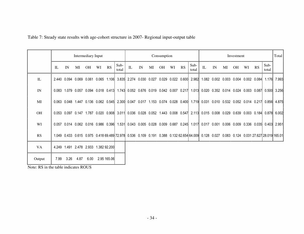
The input-output table (table 7) could be constructed by using the simulation

results of the transactions among the six regions. The IO table, which is one of the

outcomes of steady state general equilibrium simulation, is very similar to the actual IO

table presented before: (i) the industries of each state purchases the commodities from the

industries of the same state in large part; (ii) the consumers and investors also buy the

majority of their consumption and investment goods from their own states; (iii) the

volumes of production are in the order of ROUS>IL>OH>MI>IN>WI; and (iv) the usage

of each region’s output is largely consistent with actual statistics. For example,

according to the simulation result, 48.0% of IL’s output is sold as intermediate input;

37.3% as consumption goods; and 14.7% as investment goods while actual IO table

shows that 50.3% of output produced in IL are purchased for input, 40.2% for

consumption and 9.5% for investment (see table 8).

There exists a noteworthy gap in per-capita output across the regions according to

the simulation results (table 9). Simulation and actual statistics point out that the state

with the lowest per-capita output among the five Midwest states is Michigan; and the

state with the highest per-capita output is Illinois. It should be noted that one of the

reasons for the discrepancy between simulation result and actual data could be attributed

to ignoring the differences of the technology level across the regions in the simulation

model. Also the assumption that there is no external trade may bias the estimation.

Further, it is also clear that the economy of the US was not in steady state in 2007.

- 18 -

Therefore, it is only with some degree of probability that the steady-state simulation

result and the actual statistics should not be entirely consistent with each other.

The gaps of investment in physical capital and human capital play a key role in

achieving different level of per-capita output in the simulation model. Table 10 shows

that ROUS and IL invest 17.1% and 16.2% of their output while IN, WI, MI and OH

allocate only 12.2%, 13.1%, 13.6% and 14.2% of their output in physical investment.

This difference in investment tendency is related to the rate of rental return (see table 12

for factor prices): household agents would more inclined to consume the goods rather

than save and invest them when the rental return becomes relatively low (or is expected

to become low in the dynamic model.)

Also, the educational attainment could be a major factor in determining the

difference of economic performance (here, per-capita output) since the educational

investment is directly linked to the improvement of the human capital stock or

productivity in our model. It is very certain in this model that the regions with higher

per-capita output tend to combine inputs such as physical capital and labor force with a

higher level of productivity. Table 11 shows the average time share spent in educational

investment across the regions: IN, MI, WI and OH spend apparently less time in

education than ROUS and IL. Accordingly, there should be subsequent gaps in human

capital stock across the regions: figure 2 shows the discrepancies of the age-productivity

profile (or human capital stock).

There is a notable gap between two groups: high skilled region and less skilled

regions. The high skilled region are ROUS and IL; and less skilled region consist of IN,

MI, OH and WI. For example, the average worker at the retirement age in the high

- 19 -

skilled region (that is ROUS and IL) is 36.8% more productive than the worker at the

same age in the less skilled region (that is IN, MI, OH and WI). This simulation result is

consistent with the statistics of labor productivity between the regions: the labor statistics

shows that IL and ROUS is the leading region in terms of labor productivity (the last row

in table 11). Again, these gaps in productivity are attributed mainly to the differences of

time spent on educational investment (table 11) and also the level of physical capital

stock in the six-regional economies according to the model specifications (see 24).

Finally, Table 12 shows the regional prices such as output, consumption and

investment price as well as production factors. The gaps of goods prices between the

regions are larger than the actual CPI presented in the table 2. However, the order of

prices matches well with the actual CPI level except MI: The simulation results under-

estimates the consumption price in MI, compared to the table 2. Also, the simulation

results imply that renting physical capital and hiring one unit of labor cost the most in the

ROUS; on the contrary, the least region is IN.

Another steady state result can be generated with the different age-cohort

structure in order to obtain the insight of impact of population ageing on the economy.

The Census Bureau expects that the population ageing process will accelerate over time

(table 13). According to the projection of the Census Bureau, the number of people

between 15 and 64 will decline in the Midwest from 2007 to 2030. On the contrary, the

number of people above 65 will grow at a significant rate. In particular, in the ROUS, the

number of people of age 65+ will almost double from 2007 to 2030.

Without any change of model specification, the steady state simulation was

implemented with the projected age-cohort structure for the year 2030. It is very

- 20 -

important to note that this steady state result does not reflect the dynamic changes of the

human capital level of households in each region. In other words, the steady-state result

in this section reflects the changes of human capital level only between the generations,

but does not consider the changes of human capital stock along the time dimension.

However, the dynamic simulation, the result of which will be described in the next

section, will reflect the endogenous growth of human capital stock along the time

dimension as well as between the generations. Furthermore, the changes of human

capital- related variables would play a critical role in simulating the dynamics of the six

regions’ economies.

Table 14 shows the comparison of per-capita output under the two different age-

cohort structures. The results are quite intuitive: due to the population ageing, per-capita

output under the age-cohort structure in 2030 is less than per-capita output under the age-

cohort structure in 2007 in every region. It should be noticed that the per-capita output in

OH under the demographic scenario of 2030 does not decline so much from the level

under the scenario of 2007. The number of people belonging to the working age (15-64)

in OH declines faster than the other region from 2007 through 2030; subsequently the

total population size (15+) grows at only 1.4% (table 13). On the contrary, it grows at

24.6% in the ROUS and 10.6% in the WI. The relative faster growth of the external

demand mitigates the negative impact of population ageing to some extent. This positive

effect from the external economy is reflected by the relative price changes: the demand

growth from the growing population in the other regions and the limited supply of the

good produced in OH (owing to drop of labor force) causes the improvement of the terms

of trade for OH, assuming that the goods produced in each region are imperfect

- 21 -

substitutes each other. As shown in figure 3, the growth of the relative output price of

OH from 2007 through 2030 is the highest among 5 Midwest states, reflecting the

improving terms of trade for OH.

2 Results of dynamic simulation

2.1 Dynamics of age-cohort population structure

The main origin of dynamics of the regional economies in this paper should be

population ageing: in particular, the dynamic simulation is focused on the demographic

change from 2007 through 2030. The panels in figure 4 show the changes of age-cohort

structure of each region. Again note that the total population size of IL in 2007 in this

simulation is normalized to be a unit (65

, , 2007

1

1j IL g t

g

N = ==

=∑ ). It is apparent that the

population ageing process is becoming more important in every one of the six regions

from 2007 through 2030. This paper assumes that the age-cohort structure and

population size of each region after 2030 is same as those for 20303.

2.2 Outcomes

The results presented in this section should be different from what we have seen in the

previous section since the agents are assumed to react to the expectation of future price

development caused by the demographic changes in the dynamic simulation model. In

the steady-state simulation, the price variables are assumed to be constant permanently.

3 This could be strict assumption in the dynamic simulation since the individuals respond sensitively to the

movement of economic variables in the future. Thus it is quite desirable to get the projection of age-cohort

population strucuture as long as possible for the dynamic simulation like the model in this paper.

- 22 -

Table 15 shows the per-capita output in 2007 and 2030 for each region (see the

appendix for the detailed figures). Unlike the results shown in the previous section, the

dynamic simulation demonstrates that the per-capita output will grow positively even

though there will be a fast growing population ageing phenomenon. As shown in Kim

and Hewings (2010), this is because individual’s endogenous choice in educational

investment mitigates the negative effects of population ageing to some extent thru

improving the overall productivity in the corresponding economy during the transition.

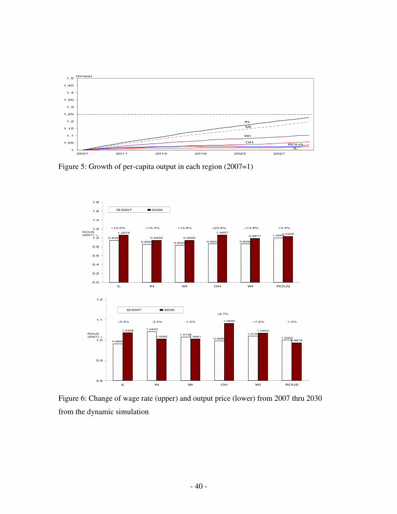
Furthermore, the simulation results projects that IN and MI will grow 22.9% and 19.6%

respectively while IL and ROUS grow at 2.2% and 3.6%. Figure 5 shows the size of per-

capita output, compared to 2007: it shows that IN and MI are growing relatively fast.

However, notice that the growth of 22.8% (IN) for 23 years (2007 thru 2030) is still very

low: it amounts to 0.9% per year. Also, note that ROUS and IL will produce most per

worker; and MI produces least per worker still in 2030 (see the appendix).

In the economy that the model describes, the physical capital and human capital

complement each other. In terms of human capital, higher human capital stock makes the

combination of labor and physical capital more effective; consequently, the combination

promotes the economic growth. This economic growth induces the physical capital stock

to be built up more since the economy produces more per unit of input than before.

However, as the physical capital stock per labor grows, the marginal return to investment

in human capital stock decreases (see the human capital technology equation 24); and

workers react less unfavorably to increasing their investment time more in their human

capital. This reluctance in increasing educational investment decelerates the economic

growth; and consequently lowers the growth of physical capital stock. Overall, in the

- 23 -

region of higher human capital stock and physical capital stock, the growth of human

capital stock and physical capital stock is relatively low. In our simulation, IL and ROUS

have the highest level of physical capital per worker and human capital among the six

regions in 2007 (see the 2nd

and 3rd

section in the table 16). On the contrary, IN and MI

have the lowest average physical capital and human capital stock, implying the marginal

return to education in IN and MI is higher than the other area. So the workers in IN and

MI will increase their educational investment more rapidly than those in ROUS and IL.

This conjecture is consistent with the simulation results: the first section of table 16

shows that educational investment in IN and MI grows at 14.2% and 12.8% respectively

while ROUS and IL grow at 1.4% and 2.4% respectively from 2007 thru 2030. Thus, the

growth of human capital stock and physical capital stock per worker in IN and MI is

higher than the other regions; and those in ROUS and IL is less than the other regions.

However, note that ROUS and IL would still lead the other regions in terms of amount of

time spent in educational investment, average human capital stock and average physical

capital stock per worker in 2030.

Population ageing will generally cause the wage rate to increase since a large

number of retired persons will cause the labor force to decline compared to the other

production factor (physical capital). Consistent with this notion, the wage rates in every

one of the six regions increases from 2007 to 2030 according to the simulation results

(see upper panel in figure 6). However, the growth rate of the wage rate is different

across the regions. For example, OH and WI are projected to experience higher increase

of wage rates than any other region. As shown in the first order condition (5), there exist

two prime forces to influencing the wage rate in each region: one is the relative scarcity

- 24 -

of labor and the other is the remaining aggregate region’s output price together with the

parameters representing the preference for each region’s output as an intermediate good.

The former is linked positively; and the latter is linked negatively with the movement of

the wage rate. First, IN, MI and WI are the top 3 regions where the labor (joined with

human capital stock) will become scarce more rapidly than the other regions (see the 3rd

section in the table 16). So the wage rate in WI is projected to show a higher growth rate

(+14.8%). However, IN and MI will not show a high increasing tendency in the wage

rate even though the labor force will become scarce relatively rapidly. This is because

their terms of trade are projected to deteriorate from 2007 through 2030. Figure 6 shows

that output price of IN, ROUS and MI will decrease 3.4%, 1.2% and 1.0% during the

period while the output price of the goods produced in OH will grow at 8.7%. The wage

rate in OH will experience the upward pressure from the improving terms of trade (which

means a decline in the relative output price in the other regions). The terms of trade of

ROUS will deteriorate since its demand for the goods produced in the Midwest states will

grow more rapidly than the Midwest states’ demand for the goods produced in ROUS,

taking the population growth projection in the table 13. However, IN and MI will receive

a smaller benefit from this declining terms of trade in ROUS since ROUS’ demand for

the goods produced in IN and MI is relatively low, compared to the other Midwest states.

Table 17 compares the preference parameter of ROUS fixed in the previous calibration

procedure (note that the elasticity of substitution across the regions was set to be identical

across the regions in the previous section). The parameters representing the preference of

ROUS for the goods produced in IN and MI as intermediate input, consumption and

investment goods are low, compared to the other regions. Also the goods produced in IN

- 25 -

and MI will be relatively abundant in 2030, compared to 2007, thanks to the rapid

increase of per-capita output in these regions as analyzed before.

V Conclusion

In the last section, the simulation results were presented to explore two issues: one is how

significantly the educational motive mitigates the negative impact of faster growing

number of elderly people (65+); and the other is how each state affects each other during

the population ageing era. According to the last section, the steady state results reveal

that each region will grow negatively in sense of per-capita output from 2007 through

2030 even though there will be some differences of degree of deterioration across the

regions.

However, dynamic simulation results imply that the economy in every region will

show the positive growth during the period thanks to a prominent underlying force of

economic growth: human capital. Also, it was shown that there exist the eventual

interactions of demographics and terms of trade of each region through the mechanisms

of demand and supply of the goods; further, these interactions substantially affect the

development of factor prices. Incorporating the information from the multi-regional

input-output within the dynamic OLG framework worked well in simulating the

mechanism of demand and supply forces at the intermediate good, consumption and

investment good markets.

This paper projects that the per-capita output of IN and MI will grow relatively

rapidly from 2007 thru 2030, taking the expected demographic developments and

- 26 -

endogenous growth mechanism into considerations. However, it should be noted that the

per-capita output simulated in the last section should be understood as a concept of

potential output: the highest sustainable level of output that the corresponding economy

can produce by efficiently combining its every inputs such as labor, capital and

technology. Thus, the simulation result regarding the growth of per-capita output just

reveals that the negative impacts of population ageing in IN and MI could be mitigated

more than the other regions due to human capital formation mechanism. To realize this

potential, it is critical that there should be no formal or informal hindrance for the

workers to implement their optimal decisions on educational investment. In practice, the

regional government should encourage the workers to invest their time in improving their

human capital stock by fiscal policy so that the economy could mitigate the negative

impact from the population ageing (see Kim and Hewings (2010) for the detailed

analysis); and follow the track presented in the last section. Meanwhile, it was shown

that IN and MI would be ones where the output price will be declining during the aging

period. The deterioration of terms of trade will result in a decline in the wage rate,

implying that the worker’s welfare would be undermined in these regions. Thus, while

encouraging the worker to invest more time in improving his/her human capital stock as

described above, the firms should try to build up the industrial relationship with the

institutions outside the Midwest so that their goods could be demanded more than before

as intermediate inputs, as well as consumption and investment goods by the regions

outside the Midwest states.

For the highly developed region like ROUS and IL in terms of per-capita physical

capital stock and human capital stock level, there exist underlying threats stemming from

- 27 -

the population ageing since the human capital growth could be sluggish in the near future

in these regions. Thus, the political effort should be concentrated on shifting the human

capital stock formation function itself. One of the policies for consideration would be

upgrading the educational environment, either through institutional or non-institutional

settings, of the group with the lower human capital stock such as international immigrants

and African-Americans. Upgrading the learning ability during the early period of life of

the people in the lower-skilled group could shift upward the post-school human capital

stock formation of the corresponding community. Kim and Hewings (2010) showed that

this kind of upgrading of human capital stock formation technology corresponding to the

African-American society in Illinois benefits the whole economic agents in Illinois

substantially in the long run under a population ageing scenario.

This paper assumes that the household agent is immobile between the states.

However, as this paper reveals in the previous section, the heterogeneous demographic

change across the regions causes the dynamic movements of factor prices and different

growth of physical and human capital stock across the regions. These effects of regional

demographic changes may provide a portion of regional residents with the incentives to

migrate between the regions to seek higher wage rates and/or higher returns to education

and so forth. Empirically, Illinois is considered to be the number two state after New

York in terms of retirement outmigration according the data analysis of 2008 American

Community Survey (ACS); and as Yu (2009) analyzed, the fund outflows stemming from

the retirement outmigration pattern negatively affect the regional economy. Thus it is

desirable to extend the model presented in this paper to incorporate the migration of

active labor and retirees. For this extension, the uninsurable idiosyncratic shock related

- 28 -

to the skill factor (say) should be included in the model; and the revealed history of

shocks makes each individual to be heterogeneous in terms of skill level. This

heterogeneity of skill level and subsequently difference of expected life-time income will

cause individuals to reveal a different pattern in choosing whether to stay or not during

each period in which the model is run. For example, one might expect that highly skilled

and unskilled workers would exhibit a different pattern of optimizing their choice on

whether to out-migrate or not. As Basile and Lim (2006) have demonstrated, there needs

to be additional consideration of the decision to migrate and the actual time when the

migration takes place. Different factors may influence each part of this two-stage process.

Finally, as mentioned before presenting the simulation results, this paper assumed

that the age-cohort population structure will be maintained after 2030. It is highly

possible that this assumption may generate a distortion of projection to some extent

especially in the later period near 2030 since the economic agents in the simulation model

optimize their choices based on the expectation of future economic variables; and future

economic variables are substantially influenced by demographics. For generating more

plausible outcomes, the longer term dynamics of age-cohort population structure in each

region should be generated. In other words, more rigorous way in obtaining the age-

cohort population structure is desired instead of depending entirely on the relatively

short-term population data provided by the Census Bureau.

- 29 -

References

Armington, P. 1969. "A Theory of Demand for Products Distinguished by Place of

Production." International Monetary Fund Staff Papers 16: 159-178.

Basile, R. and Lim, J. 2006. "Wages Differentials and Interregional Migration in the U.

S.: An Empirical Test of the "Option Value of Waiting" Theory." ERSA conference

papers, European Regional Science Association.

Bilgic, A., King, S., Lusby, A. and Schreiner, D. 2002. “Estimates of U.S. Regional

Commodity Trade Elasticities of Substitution.” Journal of Regional Analysis and

Policy 32: 79-98.

Borsch-Supan, A., Ludwig, A. and Winter, J. 2005. “Aging, Pension Reform, and Capital

Flows: A Multi-Country Simulation Model.” Computing in Economics and Finance

123: 1-49.

Bouzahzah, M., Croix, D. and Docquier, F. 2002. “Policy reforms and growth in

computable OLG economies.” Journal of Economic Dynamics & Control 26: 2093-

2113.

Fougere, M., Harvey, S., Merette, M. and Poitras, F. 2004. “Ageing Population and

Immigration in Canada: An Analysis with a Regional CGE Overlapping Generations

Model.” Canadian Journal of Regional Science 27:209-236.

Hall, R. and Jones, C. 1999. “Why Do Some Countries Produce So Much More Output

Per Worker Than Others?” The Quarterly Journal of Economics 114: 83-116.

Kehoe, T., Polo, C., and Sancho, F. 1995. “An evaluation of the performance of an

applied general equilibrium model of the Spanish economy.” Economic Theory 6:

115-141.

- 30 -

Kihoe, T. 1996. “Social Accounting Matrices and Applied General Equilibrium Models.”

Working paper 563, Federal Reserve Bank of Minneapolis.

Kim, T. and Hewings, J. 2010. “Endogenous Growth of the Ageing Economy with Intra-

Generational Heterogeneity over Race and Migration Status.” Discussion paper 10-T-

2, Regional Economics Applications Laboratory, University of Illinois at Urbana-

Champaign.

Ludwig, A., Schelkle, T. and Vogel, E. 2007. “Demographic Change, Human Capital and

Endogenous Growth.” Working paper, MEA, University of Manheim.

Miller, R. and Blair, P. 1985. Input-Output Analysis. New Jersey: Prentice-Hall, Inc.

Plassmann, F. and Tideman, T. 1999. “A Dynamic Regional Applied General

Equilibrium Model with Five Factors of Production.” Working Paper W9907,

Binghamton University.

Plassmann, F. 2005. “The Advantage of avoiding the Armington assumption in multi-

region models.” Regional Science and Urban Economics 35: 777-794.

Sadahiro, A. and Shimasawa, M. 2002. “The computable overlapping generations model

with an endogenous growth mechanism.” Economic Modelling 20:1-24.

Shoven, J. and Whalley, J. 1992. Applying General Equilibrium. New York: Cambridge

University Press.

Yu, Chenxi. 2009. “Illinois Migration Report 1992-2006.” Retrieved from

http://www.real.illinois.edu/.

- 31 -

Table 1: Expenditure quantity of each region’s industry in 2007

IL IN MI OH WI ROUS Total

I L 1,622 73 52 45 51 638 2,482

I N 55 841 42 69 14 236 1,257

M I 42 37 1,078 99 49 315 1,621

O H 35 75 110 1,310 16 529 2,075

W I 38 11 46 12 779 228 1,115

ROUS 698 337 458 715 331 40,245 42,784

Intermediate

purchases

across

regions

Intermediate total 2,490 1,375 1,786 2,249 1,240 42,192 51,333

Employee Compensation 1,742 728 1,157 1,381 699 32,459 38,166

Proprietary Income 220 81 142 138 64 4,509 5,154

Other Property Income 864 353 547 630 330 16,430 19,154

Indirect Business Taxes (A) 224 87 143 162 80 4,262 4,959

VA total 3,049 1,249 1,989 2,312 1,173 57,660 67,433

Value Added

VA total – (A) 2,826 1,162 1,846 2,150 1,093 53,398 62,474

Institutions (B) 12 9 10 13 6 196 246

Foreign Import (C) 117 88 111 141 58 5,502 6,017

Total 5,669 2,721 3,896 4,715 2,478 105,550 125,029

Total – (A) – (B) – (C) 5,316 2,537 3,632 4,399 2,333 95,590 113,807

Table 2: Consumer price index of each region in 2007

Region Coverage CPI

IL Chicago-Gary-Kenosha, IL-IN-WI 204.8

IN Cincinnati-Hamilton, OH-KY-IN 193.9

MI Detroit-Ann Arbor-Flint, MI 200.1

OH Cleveland-Akron, OH 196.0

WI Milwaukee-Racine, WI 194.1

ROUS US city average 205.7

Source: Bureau of Labor Statistics (www.bls.gov)

- 32 -

Table 3: Parameter values in production function

IL (j=1) IN (j=2) MI (j=3) OH (j=4) WI (j=5) ROUS (j=6)

IL (1 j

z ) 0.3052 0.0288 0.0142 0.0102 0.0220 0.0067

IN (2 j

z ) 0.0104 0.3314 0.0116 0.0156 0.0062 0.0025

MI (3 j

z ) 0.0079 0.0147 0.2968 0.0226 0.0210 0.0033

OH (4 j

z ) 0.0066 0.0298 0.0302 0.2977 0.0067 0.0055

WI (5 j

z ) 0.0071 0.0043 0.0128 0.0027 0.3340 0.0024

ROUS (6 j

z ) 0.1312 0.1330 0.1261 0.1625 0.1417 0.4210

Value Added (,VA j

z ) 0.5316 0.4580 0.5083 0.4887 0.4684 0.5586

Labor income share (1-j

α ) 0.6166 0.6262 0.6269 0.6425 0.6394 0.6079

Capital income share (j

α ) 0.3834 0.3738 0.3731 0.3575 0.3606 0.3921

Table 4: Expenditure quantity of each region’s consumption and investment in 2007

IL IN MI OH WI ROUS Total

Consumption

IL 1,528 35 31 25 23 342 1,984

IN 28 636 17 29 6 101 817

MI 25 15 1,029 50 22 176 1,317

OH 22 31 55 1,164 8 291 1,571

WI 26 5 28 7 622 123 812

ROUS 367 129 224 341 137 36,430 37,628

Total 1,997 851 1,384 1,616 817 37,463 44,129

Investment

IL 435 2 2 2 2 28 471

IN 7 241 9 11 2 24 293

MI 10 6 338 24 8 59 445

OH 5 7 22 350 2 59 446

WI 6 1 4 5 220 11 247

ROUS 52 23 69 74 23 9,748 9,989

Total 515 279 445 466 257 9,930 11,892

- 33 -

Table 5: Regional preference parameter values in consumption and investment function

IL (j=1) IN (j=2) MI (j=3) OH (j=4) WI (j=5) ROUS (j=6)

Consumption

IL (1,

c

jυ ) 0.7666 0.0434 0.0226 0.0160 0.0293 0.0091

IN (2,

c

jυ ) 0.0134 0.7367 0.0121 0.0176 0.0066 0.0025

MI (3,

c

jυ ) 0.0121 0.0184 0.7405 0.0311 0.0274 0.0046

OH (4,

c

jυ ) 0.0107 0.0359 0.0390 0.7113 0.0095 0.0074

WI (5,

c

jυ ) 0.0122 0.0059 0.0198 0.0043 0.7509 0.0031

ROUS (6,

c

jυ ) 0.1851 0.1597 0.1661 0.2197 0.1763 0.9733

Investment

IL (1,

I

jυ ) 0.8458 0.0072 0.0051 0.0050 0.0064 0.0029

IN (2,

I

jυ ) 0.0121 0.8562 0.0194 0.0236 0.0064 0.0023

MI (3,

I

jυ ) 0.0186 0.0235 0.7593 0.0515 0.0319 0.0057

OH (4,

I

jυ ) 0.0101 0.0234 0.0480 0.7444 0.0089 0.0057

WI (5,

I

jυ ) 0.0111 0.0028 0.0087 0.0102 0.8498 0.0010

ROUS (6,

I

jυ ) 0.1023 0.0869 0.1596 0.1654 0.0965 0.9824

Table 6: Dependency ratio of each region in 2007

IL IN MI OH WI ROUS

18.04% 18.54% 18.33% 20.11% 19.39% 18.70%

- 34 -

Table 7: Steady state results with age-cohort structure in 2007- Regional input-output table

Intermediary Input Consumption Investment Total

IL IN MI OH WI RS Sub-

total IL IN MI OH WI RS

Sub-

total IL IN MI OH WI RS

Sub-

total

IL 2.440 0.094 0.069 0.061 0.065 1.106 3.835 2.274 0.030 0.027 0.029 0.022 0.600 2.982 1.082 0.002 0.003 0.004 0.002 0.084 1.176 7.993

IN 0.083 1.079 0.057 0.094 0.018 0.413 1.743 0.052 0.676 0.019 0.042 0.007 0.217 1.013 0.020 0.352 0.014 0.024 0.003 0.087 0.500 3.256

MI 0.063 0.048 1.447 0.136 0.062 0.545 2.300 0.047 0.017 1.153 0.074 0.028 0.400 1.719 0.031 0.010 0.532 0.052 0.014 0.217 0.856 4.875

OH 0.053 0.097 0.147 1.787 0.020 0.908 3.011 0.036 0.028 0.052 1.443 0.008 0.547 2.113 0.015 0.008 0.029 0.639 0.003 0.184 0.878 6.002

WI 0.057 0.014 0.062 0.016 0.986 0.396 1.531 0.043 0.005 0.028 0.009 0.687 0.245 1.017 0.017 0.001 0.006 0.009 0.336 0.035 0.403 2.951

RS 1.049 0.433 0.615 0.975 0.418 69.489 72.978 0.536 0.109 0.191 0.388 0.132 62.654 64.009 0.128 0.027 0.083 0.124 0.031 27.627 28.019 165.01

VA 4.249 1.491 2.478 2.933 1.382 92.200

Output 7.99 3.26 4.87 6.00 2.95 165.06

Note: RS in the table indicates ROUS

- 35 -

Table 8: Percentage of usage of each region’s output (%)

Intermediary Input Consumption Investment

IL Simulation 47.97 37.31 14.72

Actual data 50.27 40.19 9.54

IN Simulation 53.54 31.11 15.35

Actual data 53.11 34.52 12.38

MI Simulation 47.18 35.26 17.56

Actual data 47.92 38.93 13.15

OH Simulation 50.17 35.21 14.62

Actual data 50.71 38.39 10.90

WI Simulation 51.88 34.47 13.65

Actual data 51.29 37.35 11.36

ROUS Simulation 44.23 38.79 16.98

Actual data 47.33 41.62 11.05

Table 9: Per-capita output

IL IN MI OH WI ROUS

Simulation 0.9704 0.8036 0.7286 0.7990 0.7996 1.0000

Actual data 1.0729 0.8885 0.8442 0.8835 0.9197 1.0000

Note: 1. Numbers of ROUS is normalized to a unit.

2. Actual data is calculated by GSP (Gross State Product) excluding public sectors ÷ population

estimation in 2007.

Source: BEA (www.bea.gov) for GSP; and Census Bureau for population estimation.

Table 10: Steady-state results- Investment-output ratio

IL IN MI OH WI ROUS

Physical Investment (A) 1.2911 0.3982 0.6625 0.8502 0.3876 28.2210

Output (B) 7.9929 3.2557 4.8748 6.0022 2.9510 165.0061

Investment-Output

ratio (A / B) 0.1615 0.1223 0.1359 0.1416 0.1313 0.1710

Table 11: Steady-state results- Time share of educational investment and average human

capital stock

IL IN MI OH WI ROUS

Time share in education (%) 13.18 10.42 10.55 11.42 10.97 13.55

Avg. human capital stock 2.27 1.77 1.78 1.94 1.85 2.39

Gross State Product / Annual

Employment: 1998 thru 20071)

80.52 67.77 74.88 68.94 65.06 78.66

Note: 1) Unit: thousand dollars chained with 2000 price level. Source: Bureau of Labor Statistics and

Bureau of Economic Analysis

- 36 -

Table 12: Steady state results- Prices

IL IN MI OH WI ROUS

Production 0.9783 0.7619 0.7611 0.8816 0.8316 1.0000

Consumption 0.9720 0.8085 0.8057 0.9010 0.8608 0.9963 Goods

price Investment 0.9701 0.7841 0.8011 0.8892 0.8457 0.9968

Rental return (physical capital) 0.0857 0.0648 0.0662 0.0723 0.0690 0.0888

Wage rate 1.5363 0.9494 0.9717 1.2228 1.1041 1.6090

Table 13: Growth of population size (age 15+) from 2007 to 2030

Age IL IN MI OH WI ROUS

15-64 0.9665 0.9873 0.9474 0.9105 0.9750 1.1163

65+ 1.5595 1.5774 1.6320 1.5261 1.7803 1.9415

15+ 1.0571 1.0796 1.0535 1.0136 1.1057 1.2464

Dependency

ratio

18.04% →

29.10%

(+11.1%p)

18.54% →

29.63%

(+11.1%p)

18.33% →

31.57%

(+13.2%p)

20.11% →

33.70%

(+13.6%p)

19.39% →

35.40%

(+16.1%p)

18.70% →

32.53%

(+13.8%p)

Source: Census Bureau’s projection

Table 14: Steady state result- Per-capita output under the alternative age-cohort structures

IL IN MI OH WI ROUS

2007: A 7.9932 6.6194 6.0017 6.5813 6.5866 8.2374

2030: B 7.3336 6.1256 5.6248 6.4631 6.1252 6.6928 Per-capita

output

B/A 0.9175 0.9254 0.9372 0.9820 0.9299 0.8125

Table 15: Per-capita output from the dynamic simulation results

IL IN MI OH WI ROUS

2007: A 7.6775 5.7624 5.3164 6.1117 5.9618 7.9339

2030: B 7.8491 7.0798 6.3597 6.4586 6.5759 8.2189 Per-capita

output

B/A 1.0224 1.2286 1.1962 1.0568 1.1030 1.0359

- 37 -

Table 16: Average physical capital per effective labor and human capital stock per labor

2007 (A) 2010 2020 2030 (B) B/A

IL 0.1204 0.1205 0.1218 0.1233 1.0241

IN 0.0967 0.1007 0.1069 0.1104 1.1417

MI 0.0980 0.1015 0.1073 0.1105 1.1276

OH 0.1073 0.1089 0.1117 0.1139 1.0615

WI 0.1022 0.1049 0.1090 0.1110 1.0861

Educational

investment

(fraction of

endowment

time)

ROUS 0.1263 0.1262 0.1269 0.1281 1.0143

IL 0.9485 0.9611 0.9971 1.0565 1.1139

IN 0.7393 0.7258 0.7733 0.8618 1.1657

MI 0.7448 0.7335 0.7800 0.8676 1.1649

OH 0.8104 0.8093 0.8414 0.9062 1.1182

WI 0.7725 0.7657 0.8049 0.8803 1.1395

Human capital

stock

(ROUS in 2007

= 1)

ROUS 1.0000 1.0236 1.0757 1.1384 1.1384

IL 0.9394 0.9251 0.9514 0.9451 1.0061

IN 0.5702 0.6696 0.8387 0.8709 1.5272

MI 0.5955 0.6834 0.8389 0.8782 1.4747

OH 0.7198 0.7487 0.8326 0.8523 1.1842

WI 0.6451 0.7075 0.8337 0.8622 1.3365

Physical

capital/effective

labor

(ROUS in 2007

=1)

ROUS 1.0000 0.9806 1.0214 1.0454 1.0454

Table 17: Preference parameter of ROUS

IL IN MI OH WI ROUS

Intermediate input .0067 .0025 .0033 .0055 .0024 .4210

Consumption .0091 .0025 .0046 .0074 .0031 .9733

Investment .0029 .0023 .0057 .0057 .0010 .9824

- 38 -

0

0.005

0.01

0.015

0.02

0.025

1 5 9 13 17 21 25 29 33 37 41 45 49 53 57 61 65

IL

IN

MI

OH

WI

Age in the model

0

0.05

0.1

0.15

0.2

0.25

0.3

0.35

0.4

0.45

0.5

1 5 9 13 17 21 25 29 33 37 41 45 49 53 57 61 65

ROUS

Age in the model

Figure 1: Age-cohort population structure

0

0.5

1

1.5

2

2.5

3

3.5

4

1 5 9 13 17 21 25 29 33 37 41 45

IL

IN

MI

OH

WI

ROUS

0

0.5

1

1.5

2

2.5

3

3.5

1 5 9 13 17 21 25 29 33 37 41 45

High-skilled region

Low-skilled region

(Age in the model)

Figure 2: Steady state results- Age profile of human capital stock

0

5

10

15

20

25

IL IN MI OH WI

(%)

.9783 → 1.1591:

18.5%.7611→ .9000:

18.2%.7619 → .8986:

17.9%

.8816→ 1.0826:

22.8%

.8316→ .9785:

17.7%

Figure 3: Percentage growth of (relative) regional output prices from 2007 to 2030

according to the steady-state simulation

- 39 -

0

0.005

0.01

0.015

0.02

0.025

1 5 9 13 17 21 25 29 33 37 41 45 49 53 57 61 65

2007

2015

2030

Age in the model

1. IL

0

0.005

0.01

0.015

0.02

0.025

1 5 9 13 17 21 25 29 33 37 41 45 49 53 57 61 65

2007

2015

2030

Age in the model

2. IN

0

0.005

0.01

0.015

0.02

0.025

1 5 9 13 17 21 25 29 33 37 41 45 49 53 57 61 65

2007

2015

2030

Age in the model

3. MI

0

0.005

0.01

0.015

0.02

0.025

1 5 9 13 17 21 25 29 33 37 41 45 49 53 57 61 65

2007

2015

2030

Age in the model

4. OH

0

0.005

0.01

0.015

0.02

0.025

1 5 9 13 17 21 25 29 33 37 41 45 49 53 57 61 65

2007

2015

2030

Age in the model

5. WI

0

0.05

0.1

0.15

0.2

0.25

0.3

0.35

0.4

0.45

0.5

1 5 9 13 17 21 25 29 33 37 41 45 49 53 57 61 65

2007

2015

2030

Age in the model

6. ROUS

Figure 4: Age-cohort population structures of the each region (to be incorporated into the

simulation)

- 40 -

1

1.05

1.1

1.15

1.2

1.25

1.3

1.35

1.4

1.45

1.5

2007 2011 2015 2019 2023 2027

IN

MI

WI

ROUS

IL

OH

(times)

Figure 5: Growth of per-capita output in each region (2007=1)

0.9442

0.8565 0.83280.8602 0.8599

1.00001.0575

0.9459 0.9462

1.0657

0.98711.0335

0.0

0.2

0.4

0.6

0.8

1.0

1.2

1.4

1.6

1.8

IL IN MI OH WI ROUS

2007 2030

ROUS

(2007) =

+12.0% +10.4% +13.6% +23.9% +14.8% +3.4%

0.9825

1.0423

1.0158

0.9960

1.0193

1.0000

1.0358

1.0065 1.0061

1.0830

1.0353

0.9876

0.8

0.9

1.0

1.1

1.2

IL IN MI OH WI ROUS

2007 2030

ROUS

(2007) =

+5.4% -3.4% -1.0%

+8.7%

+1.6% -1.2%

Figure 6: Change of wage rate (upper) and output price (lower) from 2007 thru 2030

from the dynamic simulation

- 41 -

Appendix: Key variables from dynamic simulation results

1 Per-capita output

2007 (A) 2010 2015 2020 2025 2030 (B) B/A

IL 7.6775 7.7364 7.7744 7.7934 7.7942 7.8491 1.0224

IN 5.7624 5.9814 6.2942 6.5838 6.8300 7.0798 1.2286

MI 5.3164 5.4831 5.7250 5.9501 6.1436 6.3597 1.1962

OH 6.1117 6.1815 6.2491 6.3104 6.3594 6.4586 1.0568

WI 5.9618 6.0851 6.2454 6.3742 6.4676 6.5759 1.1030

ROUS 7.9339 8.0432 8.1170 8.1429 8.1242 8.2189 1.0359

2 Fraction of time-spending in educational investment (average per worker)

2007 (A) 2010 2015 2020 2025 2030 (B) B/A

IL 0.1204 0.1205 0.1210 0.1218 0.1229 0.1233 1.0241

IN 0.0967 0.1007 0.1045 0.1069 0.1091 0.1104 1.1417

MI 0.0980 0.1015 0.1050 0.1073 0.1093 0.1105 1.1276

OH 0.1073 0.1089 0.1105 0.1117 0.1132 0.1139 1.0615

WI 0.1022 0.1049 0.1076 0.1090 0.1104 0.1110 1.0861

ROUS 0.1263 0.1262 0.1265 0.1269 0.1277 0.1281 1.0143

3 Human capital stock (average per worker)

2007 (A) 2010 2015 2020 2025 2030 (B) B/A

IL 2.2669 2.2971 2.3336 2.3830 2.4479 2.5250 1.1139

IN 1.7669 1.7347 1.7633 1.8481 1.9524 2.0597 1.1657

MI 1.7800 1.7530 1.7824 1.8641 1.9662 2.0736 1.1649

OH 1.9369 1.9342 1.9561 2.0110 2.0837 2.1659 1.1182

WI 1.8463 1.8300 1.8556 1.9237 2.0108 2.1039 1.1395

ROUS 2.3900 2.4465 2.5074 2.5709 2.6428 2.7207 1.1384

4 Rental return to physical capital

2007 (A) 2010 2015 2020 2025 2030 (B) B/A

IL 0.0932 0.0946 0.0941 0.0931 0.0931 0.0968 1.0386

IN 0.1301 0.1177 0.1058 0.0996 0.0965 0.0982 0.7548

MI 0.1222 0.1121 0.1022 0.0972 0.095 0.0976 0.7987

OH 0.0985 0.0968 0.0938 0.0924 0.0926 0.0979 0.9939

WI 0.1102 0.1039 0.0968 0.093 0.0917 0.0952 0.8639

ROUS 0.0955 0.0965 0.0948 0.0924 0.0909 0.0903 0.9455

- 42 -

5 Wage rate (before tax)

2007 (A) 2010 2015 2020 2025 2030 (B) B/A

IL 1.4393 1.4475 1.4796 1.5168 1.5477 1.612 1.1200

IN 1.3056 1.3643 1.4151 1.4248 1.4176 1.4419 1.1044

MI 1.2695 1.3234 1.3736 1.3944 1.4032 1.4423 1.1361

OH 1.3112 1.3485 1.4156 1.4747 1.5273 1.6244 1.2389

WI 1.3108 1.3475 1.3954 1.4276 1.4489 1.5046 1.1478

ROUS 1.5243 1.5138 1.5306 1.5556 1.5711 1.5754 1.0335

6 Output price

2007 (A) 2010 2015 2020 2025 2030 (B) B/A

IL 0.9632 0.9707 0.9797 0.9885 0.9991 1.0155 1.0543

IN 1.0219 1.0164 1.0060 0.9944 0.9864 0.9868 0.9657

MI 0.9959 0.9927 0.9859 0.9801 0.9787 0.9864 0.9905

OH 0.9765 0.9853 0.9995 1.0140 1.0320 1.0618 1.0874

WI 0.9993 0.9978 0.9963 0.9968 1.0011 1.0150 1.0157

ROUS 0.9804 0.9814 0.9820 0.9822 0.9832 0.9682 0.9876

7 Consumption price

2007 (A) 2010 2015 2020 2025 2030 (B) B/A

IL 0.9672 0.9731 0.9800 0.9867 0.9951 1.0053 1.0394

IN 1.0103 1.0070 1.0003 0.9926 0.9880 0.9878 0.9777

MI 0.9912 0.9895 0.9852 0.9815 0.9815 0.9864 0.9952

OH 0.9786 0.9851 0.9950 1.0050 1.0179 1.0358 1.0585

WI 0.9947 0.9940 0.9931 0.9936 0.9974 1.0060 1.0114

ROUS 0.9805 0.9815 0.9822 0.9825 0.9838 0.9695 0.9888

8 Investment price

2007 (A) 2010 2015 2020 2025 2030 (B) B/A

IL 0.9861 0.9916 0.9988 1.0060 1.0142 1.0434 1.0581

IN 1.0363 1.0307 1.0215 1.0114 1.0039 1.0196 0.9839

MI 1.0117 1.0087 1.0035 0.9993 0.9982 1.0188 1.0070

OH 0.9979 1.0035 1.0132 1.0234 1.0357 1.0723 1.0746

WI 1.0180 1.0157 1.0138 1.0140 1.0168 1.0439 1.0254

ROUS 1.0001 1.0002 1.0002 1.0002 1.0003 1.0009 1.0008

9 Social security tax rate

2007 (A) 2010 2015 2020 2025 2030 (B) B/A

US 0.1184 0.1195 0.1309 0.1457 0.1601 0.1657 1.3995