B i b l i o t h w e nationale du Canada - - -

- -

.

CANADIAN THESES ON MICROFICHE

- - - -

- NAME OF

I ZER- LIN CMhl

DEGREE FOR WH~CH THESIS WAS ~ E S E N T E D / M45TFK ciF k i ~ r \ l C l f GRADE POUR LEQUEL CETTE THESE FUT P R ~ S E N T ~ E -

I

NAME OF SUPERVISOR/NOM DU DIREC TEUR DE T H ~ S E F ~ ~ F E ~ s OR C . VZ&A 5

Permission is hereby granted to the NATIONAL LIBRARY OF , L'autorisation est, par la prgsente, accordge la BIBLIOTH~- - - P --

CANADA to microfilm this thesis and to lend or sell copips -QUE NATIONALE DU CANADA de rnicrofilrner.cette thhse et . -

of the film. de prgter ou de vendre des exernplaires du fi lm.

The author reserves other pub1 ication rights, and ne i th r the L'auteur se rgserve les autres d o i t s de publication; n i la

thesis nor extensive extracts from it may be printed or other- th8seni de longs extraits de celle-ci ne doivent &re imprimBs n

wi se reproduced wi t h w t the author's written permi ss im. / ou a-trernenr reproauits sans l'eutorisation &rite de /'auteur.

. .

National Library of Canada "' Bibliotheque nationale du Canada E

Cataloguing Branch Direction du catalogage Canadian Theses Division Division des theses canadiennes

f p - - - - - -- - - - L - L - - Ottawa, Canada K I A ON4

NOT

The quality of t h ~ s Aicrofiche is heavily dependent upon the quality of the original thegis submitted for microfilm- ing. i?ery effort has been made to ensure the.highest quality of reproduction possible.

If pages are missing, contact the university which granted the degree.

Some pages may have indistinct print especially if the or~ginal pages &re typed with a poor typewriter ribbon or if the university sent us a poor photocopy.

a

Previously copyrighted materials (journal articles, published tests, etc.) are not filmed.

Reproduction In full or in part of this fdm IS governed by the Canadian Copyright Act, R.S.C. 1970, c. (2-30. Please read the authorization forms wh~ch accompany this thesis.

La qualite de cette m~crofiche depend grandement de la qualite de la these soumise au microfilmage. Nous avons tout fait pour assurer une qualit&superieure de repro: duction.

-

S'il manque des pages, veuillez communiquer avec I'un~versite qui a confere le grade.

-- - - - -

La qualite d'impression de certaines pages peut laisser a desirer, surtout si les pages originales ont ete dactylographiees a I'aide d'un ruban use ou st I'universite

, nous a fait parvenlr une photocopie de mauvaise qualite.

Les documents qui font deja I'objet d'un droit d'au- teur (articles de revue, examens publies, etc.) ne sont pas microfilmes.

-

La reproduction, m6me partlelle, de ce mrcrofilm est soumlse B la Lo1 canadienne sur le drolf d'auteur, SRC - ' 1970, c. C-30. Veu~llez prendre conna~ssarjice des for- mules d'autorlsatlon qul accompagnent cette these

THIS DISSERTATION HAS BEEN MICROFILMED EXACTLY AS RECEIVED NOUS L'AVONS RECUE

Tzer-Lin Chen

Villanova University,

A THESIS SUBMITTED IN P W I A L FULFIUMENT OF -

mQUI.FMENTS FOR THE I1EGmE OF THE

MASTER OF SCIENCE , .

in the Department

0 f - t e

Mathematics -

@ TZER-LIN CHEN 1978

February 1978

- - - - -

All rigfits reserved. This thesis may not be reproduced in whole or in part, by photocopy or other means, without permission of the -author.

Name :

Degree: Master of Science L

_ T i t l e of Thesis: '~ormal Approximations' t o Posteripr Distributions

Examining Committee:

~hairpkrson: D r . A . <H. .~achlan

0

Y -

. Profes-. Villefas - . \

Senior Supervisoa

D r . D. M. Eaves

External Examiner

. I hereby g r a n t t o Simon Fraser Univers.i t y t h e r i g h t - t o l e n d

my t h q s i sse r ta f i on ( t h e t i t l e o f which is -shown be lowr t o users - ><

o f t h e Simon Fraser . U n i v e r s i t y , k i b r a r y , and t o make p a r t i a l o r s i n g l e

' copies o n l y f o r , such u s e r s o r . in response t o a rehues t from t h e 1 i brery: 4

of any o the r u n i v e r s i t y , o r o t h e r educat ional i n s t i t u t i o n , on its'own

C-- -I- - - -- - - 6eha1fporLT7ir on2 o f i tsuse rs ; 1 f ~ r t ~ e r a g r e e t h a f permiss ion f o r

1 t i p l e copying o f t h i s . t h e s i s f o r - s c h b l a r l y purpose? may be g r a i t e d

me o r t h e Dear+ o f . ~ i a d u a t e Studies. I t i s understood - - - - t h a t copying - -

- -

p u b l i c a t i o n of t h i s t h e s i s f o r f i n a n c i a l ga in s h a l l n d t be a l lowed -

w i t h o u t my w r i t t e n perni ission.

T i t l e o f ~ h e s i s / ~ i s s e r ' t a t i o n :

Author : . , w

( s i g n a t u r e )

(name)

~ c h e f f g ' s Theorem and the Lebesgue Dominated Convergence - + . 8 9.f%ore2 are important too l s i n the.derivation of normal approximations

- s o

d 4

t o poster-io; dis t r ibut ions. DeGroot f i r s t introduced the defini t ion of 0

supercontinuity and used the defini t ion to provide normal approximations

_ t o poster-ior- di-sk-ibuthr&h - the c a s e - of -one unknown parameter-,- -The-- -

purpose of t h i s thes i s i s t o review an a l te rna t ike approach; based on \

the lectures of Professor C. Villegas, which i s appJicabie whenever -

- - -- the re la t ive l ikelihood~fun,ction has a special . form.

he t h e s i s i s divided in to f ive chapters, the' f i r s t presenting'

* the basic theory.

r -. ( In chapter 2 we give an alte'rnative proof of ~ c h e f f i ' s Theorem

and an a l iza t ian of the Lebesgue Dominated .

Convergence Theorem. . Also cognterexamp19- t o the converse o f p-

chef •’6 ' s Theorem.

In Chapter 3 we discuss a concept o f supercontinuity tha t bas

introduced by DeGr~ot to derive normal approximations t o pgster ior 4

i ' . . - distributions,.. We o f fe r f&ur propositions which survey the bagic ~. . properties of supercontinuity. W e also i l l u s t r a t e DeGrootks n?eehod.by

five-prac&cal example.

\

- In Chapter 4 we review an a l te rna t ibe approach based on the - - - -

lectures of Professor C..Villegas. WeXlso e l ix ida te t h i s a l te rna t ive

,- --

approach by considering f ive p rac t i ca l examples. -

Fina l ly i n Chapter 5 we consider some pkoblems which a r i s e i n ' L

Y

the appl icat ion df t he methods ih time s e r i e s analysis . . . *

+

We i l l u s t r a t e t he normal approximation t o th? dis t r i l fut ions of the / parameters of ,autoregress ive processes by consideri-ng on? p r a c t i c a l

,

iv. ; /

I

f , - L r

I, wou;a- like to express my appreciati&n to Professor C. Villegas . 1 I

b

8 and Dr. P. de,'Jong far their suggestions and $help during the writing of -, - i . .

I 6 this thesis .' I- would also like to thank Mrs. Nancy Hood for -typing the

* . L \ TABLE OF CONTENTS

*, "

'T i t l e Page

i

Approval Page 'ii .%

iii

5

v J

>

' v i

Abstract . 7

Acknowledment

Table of--€ontents

cHP$TER I In t roduc t ion -

CHAPTER I1 Weak Convergence

2 .1 In t roduc t ion

3. -2.2 A P ropos i t ion ton t h e General ~ e b e s g u e ~ ~ n t e g r a l . #

* b

2.3 Convergence i n D i s t r i b u t i o n - 6 -- \

4 P

I . 1

CHAPTER I11 Dedroot ' s Normal ~ ~ @ r o x i r n i t i o n s - t o p o s t e r i o r ' ? .-

- Sapercont inui ty *

I . Solu t ions of t h e Likelihood Equatio-n . . . H . .

Normal . ~ ~ ~ r o x i m a t i o n s t o P o ~ t e r i o r - D i s t r i b u t i o n s

' ,

Examples / ' 3

Conclusions *

CHAPTER I V An Al te rna t ive ~ p p r o a c h , Z '. s -

-- --

- I -- -

Fa 21 4 .1 In t roduct ion b , . ? =

- 4.2 ~ o r r h a l Approximations t o P o s t e r i o r p i s t r i 6 u t i o n s 22 1 I 1 , ' 4.3 Examples, - ' . . I . 25 \ \ - t

\

I, . .

- v i u

I r T

4 1

' 4.4 Condlusions 32 -

CHAPTER'V Normal Approximations to the Distributi~ns of the . ,. .

ParametGrs. of Autoregressive ~ r o w s s & . Y - .

Introduction 33

Two Strong Laws of Large Numbers in Autoregressive 34 '2 ..

Processes

Example

Conclusions Conclusions . . P a . 40 . .. . i -.. i - - -

u . --41 , * . ' 2 . , I

. ,. I I

. , i

BIBLIOGRAPHY

vii

- -

CHAPTER I

INTRODUCTION

, If a random variable x , has a probability-density f (x I a) . .

which depends on a single unkhwn real valued parameter a, and n(a) is

9

the prior'density for a, then the posterior density of a, given x is

proportional to f (x I a ) n ( a ) . In other words, the po~terior~density is -

, proportional to the product of the likelihood function and the prior' 1 . -

I

density. - - * , " . -

Normal. approximations to posterior distTibutions are avai"lab1e '

L %

- in many important cases. In the derivation of these approximations,.

DeGroot (1970) uses a concept of supercontinuity. In Chapter 3 we review

DeGroot ' s approach and discuss the .concept of supercontinlity. 1

In Chapter 4 we r&ew an alternative approach based on. the - - - -

lectures of Professor C. Villegas, which is' applicable wh

likelihood function has a simple special form. In

' the methods are illustrated by several examples.

a When the observed values constitute an autoregressi~e~process, 'J 'additional problems-arisebecause of the lack of independence. Some of ,

I \

these problems are .discussed in Chapter 5 .' a

The following definitions' are used throughout: this thesis. C *

~efinition-l.,?. 1. The function' L, defined b . I 2

/ s

. n

- a p - 2 _ - -- -

- - - - - - - --

function, and its value for any a 'is called

4

-

is called the likelihood

the likelihood of a.

Definition 1.1.2. Let a denote an arbitrary parapeter and let the

likelihood function be such that %(a) = f (x I a ) . If & is a possible* '

V

ryalue of, a and & is the.maximum likelihood estimator, then the

< , j " likelihood ratio

is caued the relative liikel'ihood of E ,

CHAPTER I1 .. % 0

j J / '

, - WEAK CONVERGENCE I

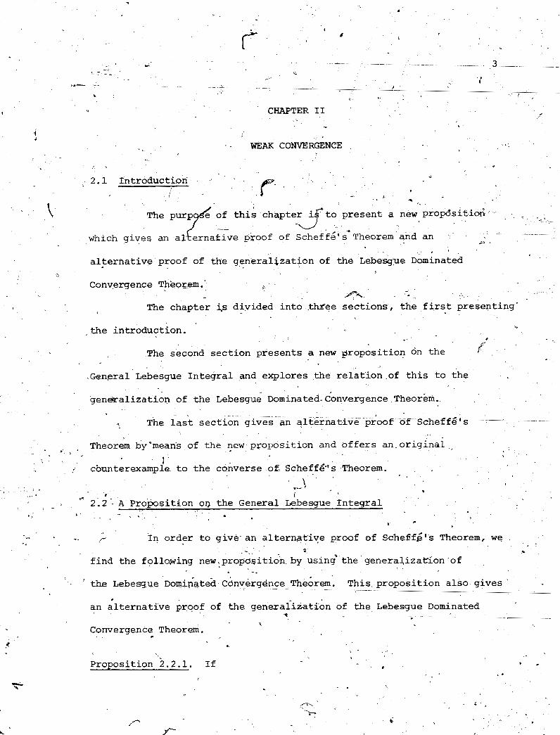
2 . 1 Introduction +

P d t * -*

'f thi; chapter i r t o present a new propdsit i& - ' 4 ,- +

-

- - proof of ~ c h e f f g ' s Theorem and an $E .

. ' a l te rna t ive proof of the general izat ion of the Lebeque Dominated

The chapter i,s divided i n t o , W e e sec t ions , the f i r s t presentingm *

I

. the introduction. +

The second sect ion presents a new groposit ion dn the f

General Lebesgue In tegra l and explores the r e l a t i o n of t h i s t o the

generalization of the ~ e b e s ~ u e Dominated- convergence he or em.

Theorem by-means of the new proposition and o f f e r s an o r ig ina l +

I *;- t

,- connterexample t o the converse of, ~ c h e f f & ' s Theorem.

\ - I . I

dr

2.2 '- A Proposition OQ the General Lebesgue In t eg ra l - *. . <

I

... - -. In order t o give an a l t e r w t i y e p r w f of ~che5fG's Theorem, we B

f ind the follo,wing new. propasitidn by usin< the generalizarion ,of - a

- * +e Lebesgue ~ o m i i a t e d cbnvi rg~nce - - - heo or em. - This - - proposit ion - a lso gives

- pp

an a l t e rna t ive prqof of the generaiizatibn t of the Lebesgue - Dominated --

* . --

Convergence Theorem.

F

Proposition 2 . 2 . 1 . I f - ,

(ii) gn 5 f n I Gn f o r a l l n a .e . - .

then / f, -+ / f and / f i s f i n i t e .

-

Proof

From Fatou ' s lemma and l i ~ sup ( - X,) . = - l i m i n f Xn --

"u:; - %+- yl

J G - / f = / l i m inf(Gn - f,) 5 l im i n f / (Gn - fn ) '

1 (2.1) l im sup / ff, 5 .I- f .

S imi la r ly ,

. . -h, - .

,- - ( 2 . 2 ) / f S l i m i n f / ' f n .

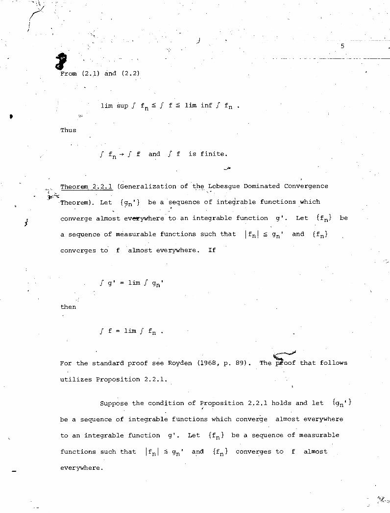
l i m sup 1 f n S 1 f 5 lim inf f, . w

Thus

. .

1 f n + J f and 1 f is f i n i t e .

- . Theorem 2 . 2 . 1 (Generalization of the Lebesgue Dominated Convergence =. - - &e

Theorem). Let { g ' } be a sequence of integrable functions which ,

converge almost eveywhere t o an integrable function g ' . Let {f,) be

a sequence of measurable functions such tha t f g and Ifn}

converges to f almost everywhere. I f

then

For the standard proof see Royden (1968, p. 89) . The tha t follows

u t i l i z e s Proposition 2 .2 .1 . I

Suppose the condition of Proposition 2 . 2 . 1 holds and l e t tgn1 1 * -

be a sequence of integrable functions which converge almost everywhere

t o an integrable function g ' . Let i f n } be a sequence of measurable

functions such tha t 1 f 1 5 g and i fn} converges t o f almost

everywhere.

I

g n S fnSG, for all n a.e.

S g n = S -9, + J - g r and - g' is finite.

I Gn = gnl -+ f g' and 1 g' is finite.

Now from Proposition 2.2.1

f, + f f and I f is finite then / f = lim f fn a

which completes the proof.

2.3 Convergence in Distribution

We apply both the notion of convergence in distribution and Scheffe's

Theorem in Chapter 3, Chapter 4 and Chapter 5. This section gives-an altexnative

proof of ~cheff6's Theorem by means of Proposition 2.2.1. This section .

also offers an original counterexample to the converse of ~cheffg's Theorem. + C

Definition 2.3.1. A sequence (F~} of distribution functions is said

to converge weakly to F if

a t a l l c o n t i n u i t y p o i n t s

Def in i t ion 2.3.2. W e say a sequence {Xn) of random v a r i a b l e s converges

i n d i s t r i b u t i o n t o t h e random v a r i a b l e X , and-we w r i t e -

i f t h e d i s t r i b u t i o n s

F o f X.

Fn of t h e Xn converge weakly t o t h e d i s t r i b u t i o n

Theorem 2-3.1. A sequence IF,} of d i s t r i b u t i o n funCtions converges I

weakly t o F i f and only i f f o r every bounded continuous r e a l funct ion h

Proof. See Kingman (1966, pp. 315-317).

Theorem 2.3.2. I f a sequence {Xn) of random v a r i a b l e s converges i n

d i s t r i b u t i o n t o t h e random v a r i a b l e X and i f f is a continuous

func t ion , then { f ( x n ) ) converges i n d i s t r i b u t i o n t o f ( X ) .

Proof. See B i l l i n g s l e y (1968, p. 31) . 4

-

Theorem 2 .3 .3 ( ~ c h e f f g ' s Theorem). If {fn} i s a sequence of p r o b a b i l i t y -- s-

d e n s i t i e s i n a Euclidean space and i f f n + f a - e . , then t h e sequence {F 1 n

of d i s t r i b u t i o n func t ions converges weakly t o F.

Proof.

J f n = l and J f = 1

J 0 + J 0 = 0 i s f i n i t e

J (f, + f ) + J 2f = 2 i s f i n i t e .

It follows from Proposit ion 2.2.1 t h a t

+ Let h be any bounded continuousreal-valued function on the

~ u c l i d e a n space on which the f n and f a r e defined.

There e x i s t s M. - ch t h a t h(x) 5 M f o r every X.

",

Hence

Thus

J hf, + ,J hf .

It io l lows from- heo or em 2.3.1 t h a t {F,) converges weakly t o F.

Remark 2.3.1. The converse of Theorem 2.3.3 i s no t t r u e , a s is shown by + .+* c

countaf&?rnple -

Figure 2.1 --

In Figure 2.1, F, (x) -+ F (x) , t h e d e r i v a t i v e s of Fn a t p o i n t s except e

jump p o i n t s a r e ze ro , b u t t h e d e r i v a t i v e s of Fn a t jump p o i n t s do n o t

e x i s t . In words, a sequence of d i s t r i b u t i o n funct ions without p r o b a b i l i t y

d e n s i t i e s can converge weakly t o a d i s t r i b u t i o n funct ion wi th a p r o b a b i l i t y

dens i ty .

--

1

CHAPTER

TO POSTERIOR DISTRIBUTIONS

The d e f i n i t i o n of supercont inui ty was f i r s t introduced by

i s an unknown parameter, observat ions

X1, . . . ,Xn form a l a r g e random sample from t h e p r o b a b i l i t y d e n s i t y

t h e p r i o r d e n s i t y of i s p o s i t i v e and continuous i n t h e

neighbourhood, supercon t inu i ty assumptions and r e g u l a r i t y assumptiom

a r e s a t i s f i e d , DeGroot ,(I9701 has shown the v a l i d i t y of normal

approximation t o t h e p o s t e r i o r d i s t r i b u t i o n of a when a i s s c a l a r .

The purpose o f t h i s chapter i s t o p r e s e n t four p ropos i t ions

which s c r u t i n i z e t h e b a s i c p r o p e r t i e s of supercon t inu i ty and t o

e l u c i d a t e DeGrootls normal approximations t o the p o s t e r i o r d i s t r i b u t i o n s

of one unknown parameter by studying f i v e p r a c t i c a l examples.

The chapter is div ided i n t o f i v e % e c t i o n s , t h e f i r s t present ing

t h e in t roduc t ion . The second s e c t i o n o f f e r s four new propos i t ions which.

survey the b a s i c p r o p e r t i e s of supercont inui ty . The t h i r d s e c t i o n deals

with s o l u t i o n s of the l ike l ihood equation when t h e observat ions

xl, . . . ,Xnform a l a r g e random sample from the p r o b a b i l i t y d e n s i t y

Sec t ion 4 i l l u s t r a t e s DeGrootls normal approximations t o t h e

p o s t e r i o r d i s t r i b u t i o n s i n t h e case of one unknown parameter. The l a s t

s e c t i o n s t u d i e s f i v e p r a c t i c a l examples which expla in DeGrootls normal

approximations t o t h e p o s t e r i o r d i s t r i b u t i o n s i n the case of one unknown

parameter.

3.2 Supercont inui ty

DeGroot (1970) f i r s t introduc-ed t h e d e f i n i t i o n of supercont inui ty .

'7 Supercontinuity is equivalent t o t h e ordinary con t inu i ty under a

- t

condi t ion which w i l l b e i l l u s t r a t e d i n Remark 3.2.1. i his s e c t i o n a l s o

p resen t s four new propos i t ions i n supercont inui ty . These p ropos i t ions

survey t h e b a s i c p r o p e r t i e s of super/ntinuity.,

~ e f i n i t & 3.2.1. Following .DeGroot (1970) a real-valued funct ion g

is supercontinuous a t t h e va lue a. € $2 i f

and g(X,a) i s s p e c i f i e d a t every p o i n t (x , a ) of t h e product space

S x 51, where S is t h e sample space of a s i n g l e observat ion X , 52 i s - -- -

an open ' i n t e r v a l of t h e r e a l l i n e and N (a0.6) i s the i n t e r v a l around

a0 conta in ing every p o i n t i n $2 whose d i s t a n c e from a. is less than

6 , and t h e expecta t ion i s computed assuming t h a t t h e random v a r i a b l e

X has t h e d i s t r i b u t i o n indexed by a. .

' Remark 3.2.1. I f EI sup / g ( x , a ) - g(x ,ao) I ] e x i s t s f o r a l l a€N (ao, 6)

s u f f i c i e n t l y small va lues of 6 , then supercont inui ty of t h e func t ion

g a t a. i s equ iva len t t o ordinary con t inu i ty of t h e func t ion g ( x , * ) . -

a t aO f o r a l l va lues of x € S except on a subset T o f S whose

5

p r o b a b i l i t y is 0.

The fol lowing four new propos i t ions survey t h e b a s i c p r o p e r t i e s

of supercontinuity.

a, Proposition 3.2.1. If g and h are supercontinu~us at the value

-P

a. C P, then' g + h is supercontinuous at the value a. C 9.

Proof. .

Hence, g + h is supercontinuous at the value a. C 9.

Proposition 3.2.2: If g and h are supercontinuous at the value

a C Q , and there exists M > 0 such that ~ax(~~(x,a)I,lh(x,a~)I) 5 M 0

for all values of a € N(a0,6) and for all values of x C S, then gh

is supercontinuous at the value a. C P.

Proof. ', -

Hence, i s s ~ p e r ~ ~ n t i n ~ ~ ~ ~ a t t h e va lue a. ~ ' 8 . .

* 5

I f h is supercontinuous a t &e value -ao E 51; And

/ t h e r e e x i s t s K > 0 such t h a t Ih (x,a) ( 2 K f o r a l l va lues of -

Jl a E N(a0,6) and f o r a l l va lues of x E S , then - i s supercontinuous h

B \

a t t h e va lue a. C Q.

Proof.

1 Hence, - i s supercontinuous a t 'the value a. t 51. h

d

em ark 3.2.2. Crarner (1946, pp. 67-68) has s t a t ed the following r e su l t : /

I f f o r almost every value of x t S and f o r a f ixed value a. of a ,

the followinq conditions a r e sa t isf ied: '

(i) The p a r t i a l der iva t ive e x i s t s ,

I -, g(x , a + h) - g(x,a)

(ii) ye have h < G ( x ) f o r

u 0 . c ihl c hot where ho i s independent of . A x , and G is an integrable

function over S with . respec t t o probabi l i ty dens i ty f (x I ao ) and S . ,

is the sample space, then

-,

-. : . F-, 4

Proposition 3.2.4. S f (ii) i n em ark -

a - Pr ' ag(x ta ) f ( X 1 ao)dp (x) 1 {z is 9 b . a ) f (X I-ao)dlJ (x) } = { I S -7 a=ao a=ao .

supercontinuous a t the value uO .

Proof.

I

..- , - 'if:

Hence, g i s supercontinuous a t the value a. . - 1 5 +-

.?.

\

\ - - y

3.3 Solutions of the Likelihood Equation d

-

1 We now proceed t o . f i n d the solutions of the l ikelihood

equation,when the observations X , . . . X form a large random sample ( 1

from the probabi l i ty density f ( a 1 ao) . 'i

make the following assumptions (primes ind ica te

d i f f e r e n t i a t i e h respect t o a only) : -

Assumption L 1 . The second-order der ivat ives f " (x 1 a) e x i s t fo r a l l

values of k € S and a l l values of a i n sdme neighbourhood N (a0,6) - of a. t where 6 > 0.

Assumption LZ . JSr f (X 1 ao) dp (x) .= 0 . and IS f" (x / ao) du (x) = 0.

Assumption L3 . For any values of x E S and a C ~ ( a 0 , 6 ) , it i s , .

assumed t h a t f (x I a ) > 0. Furthermore, i f h ( x I a) is de'f ineb by

+'.

it is assumed t h a t functions A, A ' and 1" are superc continuous a t ,

=0. and f o t a l l va lues of a € N ( C C ~ ~ ~ ) , t h e expecta t idns E'[X(x I a ) 1 ;

EIX1'(x, ta) l a r e . f i n i t e , where t ,

' Assumption L4 . For -any va lues a € N ($ ,6) , l e t IYa) . be dkf ineg a s

f 01 lows :

The unct ion I i s p o s i t i v e and cont$nuous throughout t h e .L 0

lieo or em 3.3.1. I f a. is an unknown parameter, observat ions P -

x l , . . . ,Xn form a random sample from the p r o b a b i l i t y denb i ty - - .r:, $-* !%

f(* 1 a o ) , and Assumptions L1 t o Lq a r e s a t i s f i e d , then , wi th

p r o b a b i l i t y 1, t h e r e w i l l e x i s t an i n t e g e r no such t h a t f o r each value

of n 2 no , t h e l ike l ihood equation

n (3.3) 1 X' (xi I a) = o

i=l

= log f (x I a)

h a s a s o l u t i o n a - . . . , and l i m & ( x l , . . . rXn) = a o - ir n-

Proof. See DeGroot (1970, pp. 209-2101,

If a. is an unknown parameter, observations X i , . . . ,xn -

form a large random sample from the probabi l i ty densi ty f ( 1 ao) , the ,

p r i o r dens i ty of a i s pos i t i ve and continuous i n the neighbourhdod

N(a0,6) , and Assumptions Li t o Lq are s a t i s f i e d , DeGroot '(1970)

has shown t h a t t he pos te r ib r d i s t r i b u t i o n of a i s approximately a - . . 1 normal d i s t r i bu t ion with mean 2 and variance I where

C

t X I . . . X denote so lu t ions of the likel$hood equation (3.3) and -2

3.5 Examples

This s,ectiop i l l u s t r a t e s DeGYoot's normal approximations t o the IC

d i s t r i bu t ions by considering f i v e p r a c t i c a l exampLes. - -

Example 3.5.1. Suppose t h a t X I . . . X is a random sample from a

Bernoulli d i s t r i bu t ion with an unknown-value of t he parameter

(0 < a < 1).

s a t i s f i e d It can be che,cked t h a t ' Assumptions L1 t o L4 + a r e .r

and -

I 4

I t a l so can be checked t h a t the normal approximation t o the '

-=- - pos.terior d i s t r i bu t ion of a is a normal d i s t r i bu t ion with mean x

,"

- - ' and variance x ( 1 - X) .

n

Example 3.5.2. Suppose that X I . . . X is a random sample from a

binomial d i s t r i b u t i o n with an unknown value of t he parameter a

I .

( 0 < a < 1)

It can be cheyked t h a t Assumption3 L1 t o L4 a r e s a t i s f i e d and

It a l s o can be checked t h a t the normal approximation t o the -

and pos te r io r d i s t r i bu t ion of a i s a normal d i s t r i bu t ion with mean - m

T-u

Example 3.5.3. Suppose t h a t X , . . . X is a random sample from a

Poisson d i s t r i b u t i o n with an unknown value of the mean u (a > 0 ) .

It can be checked t h a t Assumptions L1 t o L4,are s a t i s f i e d and

It a l s o can be checked t h a t the normal approximation t o the - -

- pos te r io r d i s t r i bu t ion of a is a normal d i s t r i bu t ion with mean x and

- X variance n.

Exainple 3.5.4. Suppose t h a t X I . . . X i s a random sample from a

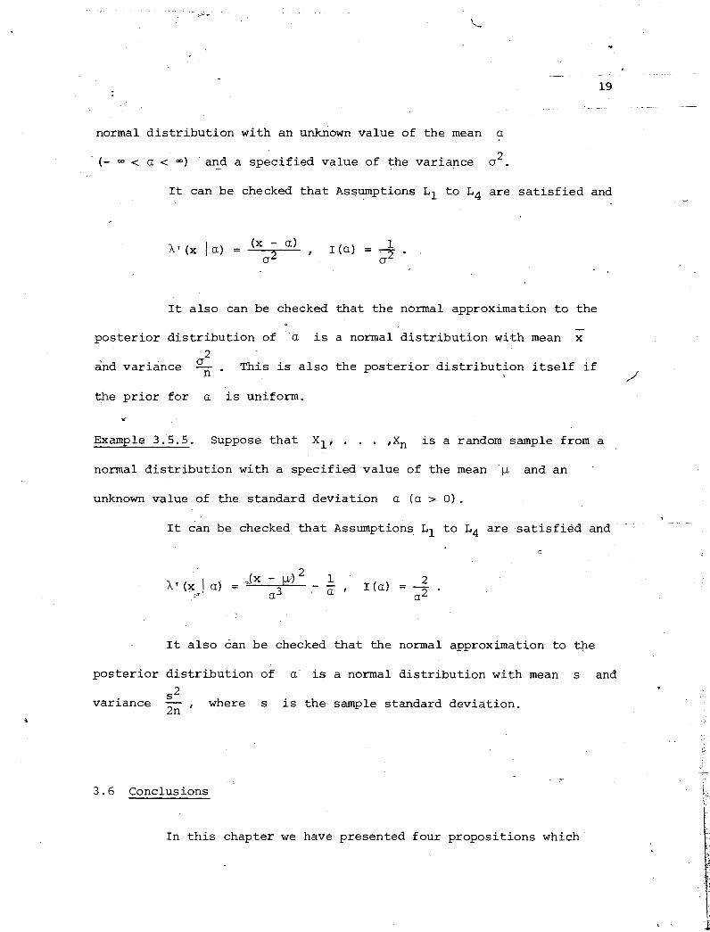
normal d i s t r i bu t ion with an unknown value of the mean a

- 2 (- < a < a) and a specif ied value of the variance o .

It can be checked t h a t Assumptions L1 t o Lq a re s a t i s f i e d and -

It a l so can be checked t h a t the normal approximation t o the

- pos te r ior d i s t r i bu t ion of a is a normal d i s t r i bu t ion with mean x

2 &d variance 7 . This is a l s o the poster ior d i s t r i bu t ion i t s e l f i f

/' the p r io r fo r a i s uniform.

Example 3.5.5. Suppose t h a t is a random sample from a

normal d i s t r i bu t ion with a specif ied value of the mean p and an

unknown value of the standard deviation a (a > 0 ) .

It can be checked t h a t Assumptions Ll t o L4 a re s a t i s f i e d and

It a l s o can be checked t h a t the normal approximation t o We

pos te r ior d i s t r i bu t ion of a is a normal d i s t r i bu t ion with mean s and rn

variance - where s i s the sample standard deviation. 2n '

3.6 Conclusions

In t h i s chapter w e have presented four proposit ions which

scrutinize the basic properties of supercontinuity and we elucidated

DeGrootrs normal approximations to the posterior distribution of one

unknown parameter by studying five practical examples.

CHAPTER ' IV

AN ALTERNATIVE APPROACH 0

4.1 In t roduc t ion

I n t h e p r e s e n t chapter we review an a l t e r n a t i v e approach t o

t h e problem of f i n d i n g normal approximations t o p o s t e r i o r d i s t r i - -

bu t ions t h a t was developed i n the l e c t u r e s o f P ro fessor C. *

Vi l l egas . We assume t h a t t h e unknown parameter a is a column vec to r - -

belonging t o a known open set B i n a p-dimensional space. The b a s i c

assumption i s t h a t , f o r s u f f i c i e n t l y l a r g e n,, t h e r e l a t i v e l ike l ihood

func t ion has t h e s p e c i a l form exp[- ncp(&,un(X1, ; . . , X n ) ) I r where - cp i s a known func t ion of two arguments,. a parameter 6 f 51 and a - vec to r un which i s a known func t ion of t h e observat ions . We assume - a l s o t h a t , wi th p r o b a b i l i t y 1, t h e r e i s , . f o r a s u f f i c i e n t l y l a r g e sample - -

s i z e ' n , a uniquely def ined maximum l ike l ihood es t ima te which - converges t o t h e t r u e parameter a when n inc reases i n d e f i n i t e l y . - F i n a l l y , w e assume t h a t cp i s a twice -d i f fe ren t i ab le func t ion of E -

when X l r . - . , X n a r e f i x e d , and t h a t , wi th p r o b a b i l i t y 1, '

u . . . , c o n v g e s t o an unknown vec to r u. - - i !

The purpose of t h i s chapter is t o review an a l t e r n a t i v e , , I I

approach, under P ro fessor C . V i l l egas ' s assumptions. These normal L

- + approximations t o p o s t e r i o r d is t r ibutCons are obta ined by applying f

the Taylor expansion technique , t h e s t rong law of l a r g e numbers and i

+.

scheffg's Themem respective* to a special form of reIal9ve Iikellihood. Tn - t

P the alternative approach we do not apply DeGro t's supercontinuity notion.

This chapter is divided into thre sections, the first <

presenting the introduction. The second section reviews an alternative

approach of normal approximations to posterior distributions - under

Professor C. Villegas' s assumptions. The last section elucidates these normal A:+.

i ,-

approximations to posterior distributions by considering five practical 1 -

Normal Approximations to Posterior Distributions

Suppose these assumptions in 4.1 hold. It follows from

Definition 1.1.2 that

Hence

Maximizing exp[- rxp(&,un(Xl, . . . ,Xn))l is equivalent to - -. - minimizing rp ( E r ~ ( x 1 , . . . ,Xn) 1 , it follows that

II

, A second-order Taylor expansion gives, assuming t h a t - and

& a r e column vec tors , ) -

/' The prime denotes t ransposi t ion and 4 i s t he matrix whose i , j - t h -

3 - ' entry i s ( p i j (2 - + 8 (5 - - - GI, un(xl, . . . , x n ) ) = -

+ g(& - &) , u n ( ~ l , . . . , x n ) ) f o r some 0 i n t he i n t e r v a l - - 3aiaa

j O < 0 c 1.

We define An t o be the upper t r i angula r matrix with pos i t ive

diagonal elements which i s uniquely defined by t

,., I

For f ixe2 vector - T suppose t h a t - a i s specif ied by the equation

Hence

. , Let n ( a ) - be the p r i o r f o r the parameter a. Since the Jacobian -

- ~- -- ~ -

a i J = I I is constant, the p r io r fo r - T w i l l be proportional t o

A n ( 2 - + nn-l ) . Assuming t h a t with probabi l i ty 3, -+ ,,y follows

-- .

. '

t ha t the p r io r density fo r r converges t o a constant. We also have, -

with probabi l i ty 1,

d and . .

.An + A where A 'A = 4 .

Therefore, fo r any fixed , A - converges t o the iden t i ty matrix - - <

with probabili ty 1. Hence

= exp 1- i l r~d-l+n~n-lr) 2 - I

converges, with probabili ty 1, t o

This provides an approximation t o the r e l a t ive l ike l iho

values of n.

w The normal approximation t o the posterior d is t r ibut ion of a - .-.

i s thus a norma1,distribution with mean vector a and covariance matrix -

4.3 Examples

We illustrate the normal approximations to posterior

distributions by considering five practical examples.

Example 4.3.1. Suppose that X1, . . . ,X, is a random sample from a - d .

normal probability , distribution. C

The maximum likelihood estimates are

The relative likelihood is

where

It is well known that, with probability 1,

It can be checked that the matrix 4 is

It is obvious that

It is clear that the relative likelihood is approximately the density

of a normal distribution with mean zero and covariance matrix 6-I . - n

In other words, the normal approximation to the posterior distribution

- of (al .a2) is a normal distribution with mean vector (x,s) and

covariance matrix [n; I -'.

Example 4.3.2. Suppose that X , . . . X is a random sample from a

Rayleigh distribution

,-

la) = { , ,

({exp[- x2/~a21)x/a2 for x + 0

The maximum likelihood estimate is

It can be checked that

It is well known that Ci?

with probability 1. It also can be checked that

where cpW(a,un(X1, . . . , X n ) ) = aLcp(a,un(x1, . . . ,x,)) .

It i s c l ea r t h a t t he r e l a t i v e l ikelihood is approximately a normal

2 d i s t r i bu t ion with mean 0 and variance . In o ther words, the normal

4

approxtmation t o the pos t e r io r d i s t r i bu t ion of a i s a normal

A 2 a d i s t r i bu t ion with mean a and variance - .

4n

Example 4 . 3 . 3 . Suppose t h a t X , . . . X is a random sample Trom a

Poisson d i s t r i bu t ion

(d

The maximum l ikel ihood estimate i s

It can be checkkd t h a t

- un (XI r . . t X n )

+ un ( X I , . . . , X n ) log un (XI , . . . , X n )

t

n where u,(X1, . . . , X n ) = [ 1 Xi] .

i=l n

I t i s well known t h a t

n un ( X l , . . . , X n ) = [ 1 Xi] + E [Xi] = a with probabi l i ty 1.

I t a l so can be checked t h a t

2 where cp" (a,u,(xl', . . . ,xn) = a .cp(a,un(X1, . . . ,xn)

a a2

I t i s c l ea r t h a t the r e l a t i v e l ikelihood is approximately a normal

- d i s t r i bu t ion with mean 0 and variance. x. In other words, the normal

approximation t o the pos te r io r d i s t r i bu t ion of a is a normal

- - X d i s t r i bu t ion with mean x and variance -. I n

3 I:

> Example 4.3.4. Suppose t h a t X , . . . X is a r dom sample from a

- L + f - -

Bernoulli d i s t r i bu t ion

. - 4--

f ( x I a) = a X ( l -- a) l-x f o r x = , 0 , 1 .

The maximum likelihood estimate is

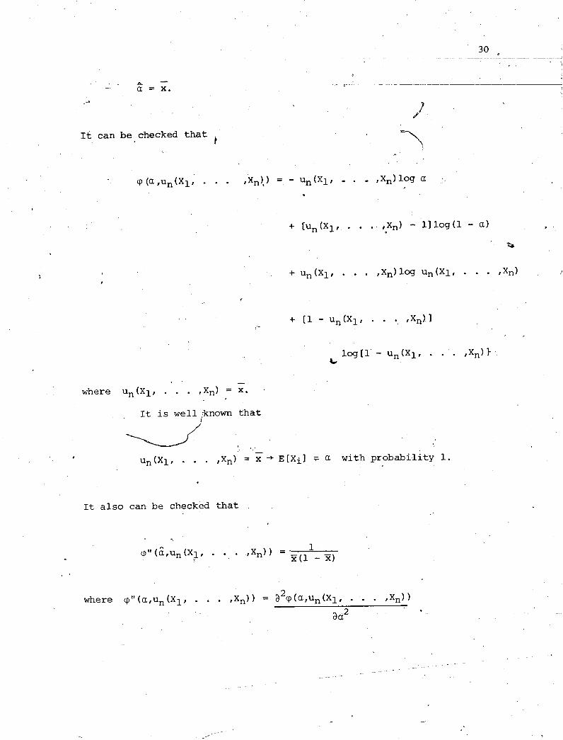
~t can be checked t h a t I

cp (a ,u, (xl, . . . , x ~ ) , ) = - un (Xl . Xn) log a '.

. - - where un ( X l r . . . , X n ) = x. '

It is w e l l ;known t h a t i

' . - un[xlr . . . ,xn) = x -+ E [xi] 7 a wi th p r o b a b i l i t y 1.

It a l s o can be checked that

2 where cp"(a,un(X1, . . . rxn)) = a cp(afun(X1, . - . ,Xn))

a a2

It is clear that the relative likelihood is approximately a normal 3 1

- - distribution with mean 0 and variance x(1 - x)'. In other words, the

normal approximation to the posterio 4 distribution of a is a normal

- - - distribution with mean x and variance x(l - x) .

n -7

Example 4.3.5. Suppose that X1, . . . ,Xn is a random sample from an

exponential density - L - - --

otherwise.

The maximum likelihood estimate is

It can be checked that

It is well k n m that

T -.., 9 -;"&>: I t a l s o can be checked t h a t -<a f -.*+

..=

a2,(a,un(xl, . . . ,X,U . where 9" (a,un(xl , . . - ,Xn) ) = -

It i s c l e a r t h a t t h e r e l a t i v e l ike l ihood is approximately a normal

- 2 d i s t r i b u t i o n wi th mean 0 and va r i ance (x) . I n o t h e r words, the

normal &proximation t o . t h e p o s t e r i o r d i s t r i b u t i o n of a i s a normal

- - 2 d i s t r i b u t i o n wi th mean x and va r i ance (x) .

n

4.4 Conclusions

I n this chapter w e review an a l t e r n a t i v e approach under

P ro fessor C. V i l l e g a s ' s assumptions. I n t h e a l t e r n a t i v e approach

w e d i d n o t apply DeGroot ' s supercon t inu i ty not ion .

NORMAL APPROXIMATIONS TO THE DISTRIBUTIONS OF THE

5.1 Introduction

PARAMETERS OF AUTOREGRESSIVE PROCESSES

I n this

approximations t o

chapter we donsider the problem of f inding asymptobic

t he pos te r ior d i s t r i bu t ions of the parameters of

autoregressive processes. I n the examples qf Chapter 3 and 4 we applied

the ordinary strong law of la rge numbers, but the ordinary strong law of -

large numbers does not apply t o aut!oregressive processes, and a version

of the s t rong law of la rge numbers val id f o r autoregressive processes

should be used instead.

The purpose of t h i s chapter i s t o e lucidate the normal

approximations t o t he d i s t r i bu t ions of the paraineters of autoregressive -

processes by studying one p rac t i ca l example. The normal approximations *

t o - t h e d i s t r i bu t ions of the parameters of autoregressive processes a re

obtained by applying s t rong law of large numbers t o the

conditional r e l a t i v e l ikelihood.

This chapter is divided i n t o three sect ions , the f i r s t

introducing the topic . The second sect ion s t a t e s two s t rong

laws of large numbers. The l a s t section considers one p rac t i ca l .

example which describes the normal approximations t o the d i s t r ibu t ions - -

o f - t h e parameters of autoregressive processes.

5.2 Two Strong Laws of Large Numbers in Autoregressive Processes

N ~ W we shall state two stronG laws of large numbers.

We shall use the foilowing definition.

% Definition 5.2.1. We call the following equation the first-order

p-component vector autoregressive process. a

where

a i s a p x p -

Theorem 5.2.1.

matrix of coefficients, E [Vt] =&0 , E [V~V;] = Z. - - * If- Xt is defined by (5.1), t = 1 2 . . . . , with. - a - -

having eigenvalues less than 1 in absolute value, and if Vtts are 4 -

independently and identically distributed with EIVtl = 0 and .+ .. ?.* $1,- - $ * . ' L.i$

E [V~V;] = Z, then with probability 1 h -

Proof. See Anderson (1971, p. 195) .

Theorem 5.2.2. Under t he condit ions of Theorem

pos i t i ve d e f i n i t e , then with probabi l i ty 1

5.2.1 and i f D i s s

where

ti"

Proof. See Anderson (1971, p. 196) .

Example

We i l l u s t r a t e t he normal approximations t o the d i s t r i bu t ions

of the parameters. of autoregressive processes by considerjng the following

simple example: I

Let Xi denote t he autoregressive process s a t i s fy ing the

following f i r s t - o r d e r s t o c h a s t i c d i f f e r e n c e equat ions :

where o is unknown, Vi is normal ( 0 , l ) .

The cond i t iona l d e n s i t y of X1 given Xo i s

and s i m i l a r l y f o r t h e cond i t iona l d e n s i t y of X given j

X j - l l X j - 2 t . - ' X1 such t h a t , f o r example t h e cond i t iona l dens i ty -

of X given X X - l r . . - l X i s n n:l

I t can be' checked t h a t t h e j o i n t cond i t iona l dens i ty of

X I , . . ,Xn given Xo i s , b

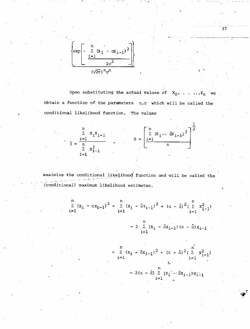
Upon substituting the actual values of Xo, . . ..,Xn we

obtain a function of the parameters a,o which will be called the

. conditional likelihood function. The values

maximize the conditional like>hoodC function and will be called the -

- - - - -- -

- - (conditional) maximum likelihood estimates.

Hence the conditional likelihood is proportional to .

*

f - It follows that the' conditional relative likelihood is equal to

J

Here we have set

It follows from Theorem 5.2.1 that d .

n 2 2 I

u x , . . . x = ( Z , --+ E with probability 1. ~t

i=l - - n

It follows from Theorem 5.2.2 that

A

a -+ a with probability 1

6 -+ o with probability 1.

I

A posterior distribution of the parameters ..9 a and o may be

derived by multiplying the conditional likelihood function by a prior

density, and we can find an approximation to this posterior distribution

using the approach developed in the previous chapter. 4 The results are

Formally the same as in simple regression. In this approximation to the

posterior distribution of a and o, these parameters, are independent, A 2 rf w

h

a has a normal distribution with mean a. and variance n . ' .-. i=l ,

and o has a normal distribution with mean a and A 2 -

=,. o variance - . 2n

parameters

strong law

normal approximations to the distributions of the .

autoregressive processes are obtained by L applying the

large numbers to the conditional relative likelihood.

BIBLIOGRAPHY

1. Anderson, T. W., The Statistical Analysis of Time Series, John Wiley and Sons, Inc., New York, 1971.

2. Billingsley, Patrick, Convergence of Probability Measures, John Wiley and Sons, Inc., New York, 1968.

Methods of Statistics, Princeton

4. DeGroot, Morris H., Optimal Statistical Decisions, McGraw-Hill Book Company, New York, 1970.

5. Kingman, J. F. and Taylor, S. J., Introduction to Measure and Probability, Cambridge University Press, 1966.

6. Royden, H. L., Real Analysis, The Maanillan Company, 1968. a