ice-ex heat exchanger analyses for ice storages in solar ... · final report november 7, 2017...

Federal Department of theEnvironment, Traffic, Energy and Communications DETEC

Swiss Federal Office of EnergyEnergy Research

s

Final Report November 7, 2017

Ice-Ex

Heat Exchanger Analyses for Ice Storages inSolar and Heat Pump Applications

Untersuchung vonEisspeicher-Warmeubertragern furSolar-Warmepumpen-Heizungen

Contracting body:

Swiss Federal Office of Energy SFOEResearch Programme Solar Heat and Heat StoragesCH-3003 Bernwww.bfe.admin.ch

Contractor:

Institut fur Solartechnik SPF, Hochschule fur Technik Rapperswil HSROberseestr. 10CH-8640 Rapperswilwww.spf.ch

Authors:

Dr. Daniel Carbonell, [email protected] Battaglia, [email protected] Philippen, [email protected]. Michel Haller, [email protected]

SFOE Head of domain: Andreas Eckmanns, [email protected] Programme manager: Dr. Elimar Frank, [email protected] Contract number: SI/501235-01

The author of this report bears the entire responsibility for the content and for the conclusionsdrawn therefrom.

Abstract

The combination of solar thermal and heat pump systems with ice storages, the so-called solar-ice systems,are becoming popular in Switzerland for the provision of space heating and domestic hot water. Thesesystems can have a high efficiency, in the range of ground source heat pumps (GSHP) or higher, withoutbeing submitted to regulations of ground water protections. However, today’s system cost are stillhigher than those from GSHP and research is needed to make solar-ice systems more efficient and costcompetitive.

One approach to improve the efficiency and the investment cost of solar-ice systems is to optimize the heatexchanger area in the ice storage. Besides the aims of increasing the efficiency and reducing installationcost, an appropriate heat exchanger design can increase the ice fraction. The aim of the present projectis to find suitable heat exchanger types and define the optimum heat exchanger area needed in the icestorage based on energetic and cost indicators.

This report is separated into six main chapters. Besides the first (Introduction) and the last (Conclusions)chapters, the report has four main chapters. Experimental results of different heat exchangers, i.e.capillary mats, flat plates and coils are presented in chapter 2. The mathematical description of an icestorage model able to cope with all experimentally analyzed heat exchangers is presented in chapter 3.In chapter 4, results from the validation of the model using the experimental data from chapter 2 areshown. The optimum heat exchanger area for the most promising heat exchangers was evaluated from asystem perspective in terms of energetic efficiency and heat generation cost. The energetic simulationsof the complete solar-ice system with varying heat exchanger type and area for different collectors areasand storage volumes is presented in chapter 5. In the same chapter, the cost effective heat exchangerarea was evaluated and compared with state of the art ground source heat pump systems.

The main conclusions of this project can be summarized as follows. Very high ice fraction can be reachedwith all heat exchangers and the casing did not show any damage under high ice fraction conditions.This means that designing an ice storage able to reach an ice fraction up to 95% or higher should besafe. Therefore, the size of the ice storage, and thus the cost of the system, have the potential to bereduced. From all the heat exchanger analyzed, the most promising designs for small ice storages (below5 m3) are polypropylene capillary mats (CM) and flat plates (PF) of stainless steel. From these twoheat exchangers, capillary mats showed the best performance considering energetic and cost indicators.Solar-ice systems using ice storages volumes from 0.3 to 0.5 m3 per MWh of yearly heating demand, andselective uncovered collectors with 1.5 to 2.5 m2/MWh in the city of Zurich were able to achieve systemperformance factors SPFSHP+ ranging from 3.5 to 6 with both CM and FP in a single family housewith 10 MWh of yearly demand. Considering the cost of the system, only simulations with CM wereable to achieve lower heat generation cost than that of the GSHP with higher SPFSHP+ (an SPFSHP+

of 4 was assumed for GSHP). For example, a system with a collector area of 1.5 m2/MWh and an icestorage volume of 5 m3/MWh, can reach heat generation cost of 29 Rp./kWh, 0.5 Rp./kWh below theGSHP reference cost, with an increase of SPFSHP+ of 20 % respect to the GSHP system. However, theretargets can only be achieved using CM and with the appropriate heat exchanger area. The optimal heatexchanger area was found to be around 5 to 6 m2 per m3 of ice storage for CM and around 10 to 12m2/m3 for FP. These heat exchanger ratios correspond to a distance between heat exchangers of around12 - 17 cm for both CM and FP. These results were obtained assuming a conservative maximum icefraction of 80 %.

Zusammenfassung

Die Kombination von solarthermischen Warmepumpensystemen mit Eisspeichern, sogenannte solare Eis-speichersysteme, findet in der Schweiz immer mehr Beachtung. Diese Systeme konnen Raumwarme undBrauchwarmwasser mit vergleichbarer oder hoherer Effizienz wie Erdsondenwarmepumpen zur Verfugungstellen. Allerdings sind die aktuellen Systemkosten im Vergleich nach wie vor hoher, weshalb Forschungs-und Entwicklungsarbeit notig ist, um solare Eisspeichersysteme effizienter und wirtschaftlich konkur-renzfahig zu machen.

Ein Ansatzpunkt zur Steigerung der Effizienz und der Wirtschaftlichkeit sind die im Eisspeicher verwen-deten Warmetauscher. Neben einer erhohter Effizienz und gunstigeren Beschaffungskosten kann ein gutesWarmetauscherdesign auch den maximal moglichen Vereisungsgrad verbessern. Das Ziel des in diesemBericht beschriebenen Projekts ist, geeignete Warmetauschergeometrien und -materialien zu identifizierenund die optimale Warmetauscherflache in Abhangigkeit von energetischen und okonomischen Zielfunk-tionen zu definieren.

Dieser Bericht ist in sechs Kapitel unterteilt. Das erste Kapitel gibt eine Einfuhrung ins Thema.Die Schlussfolgerungen aus den Arbeiten sind im Kapitel 6 zusammengefasst. Die einzelnen Arbeits-schritte sind in den Kapiteln 2 bis 5 genauer beschrieben. Die experimentellen Resultate der unter-suchten Warmetauschertypen (Kapillarmatten, Warmetauscherplatten und Wendelwarmetauscher) sindin Kapitel 2 aufgefuhrt. Das mathematische Modell, welches auf der Basis der Experimente entwickeltwurde, ist in Kapitel 3 beschrieben. In Kapitel 4 ist die Validierung des Modells mittels Daten aus denLabormessungen gegeben. Die Systemsimulationen des kompletten solaren Eisspeichersystems werden inKapitel 5 prasentiert. Die optimale Warmetauscherflache wird dabei aus der Systemperspektive in Bezugauf Energieeffizienz und Warmegestehungskosten bestimmt. Zusatzlich werden die erreichten Werte desEisspeichersystems mit heutigen Erdsondensystemen verglichen.

Die Resultate des Projekts konnen folgendermassen zusammengefasst werden: Sehr hohe Vereisungsgradewurden mit allen Warmetauschertypen erreicht, wobei der Eisspeicherbehalter in keinem ExperimentSchaden genommen hat. Daraus lasst sich schliessen, dass in einem geeigneten Behalter Vereisungsgradevon 95 % moglich sind, ohne dass Schaden zu erwarten sind. Der Verzicht auf nicht genutztes Eisspe-ichervolumen ist folglich eine Moglichkeit zur Kostenreduktion. Von den ausgemessenen Warmetauscher-typen zeigten Kapillarmatten und Warmetauscherplatten aus Edelstahl die beste Performance fur kleineEisspeicher mit einem Volumen von unter 5 m3. Die besten Resultate betreffend Systemeffizienz undKosten weissten dabei Kapillarmatten aus. Solare Eisspeichersysteme mit Eisspeichervolumina von 0.3bis 5 m3 pro MWh jahrlicher Warmebedarf und unabgedeckte Kollektoren mit einer Gesamtflache von1.5 bis 2.5 m2/MWh zeigten in den Simulationen mit Kapillarmatten und Plattenwarmetauschern Sys-temjahresarbeitszahlen SPFSHP+ von 3.5 bis 6. Die Resultate wurden fur ein Einfamilienhaus mit 10MWh jahrlichem Warmebedarf unter den klimatischen Bedingungen von Zurich generiert. Mit Blick aufdie Wirtschaftlichkeit konnten lediglich mit Kapillarmatten Simulationsbedingungen gefunden werden,welche einen hoheren SPFSHP+ bei im Vergleich mit Erdsondensystemen geringeren Kosten ermoglichten.Beispielsweise hat ein System mit einer Kollektorflache von 1.5 m2/MWh und einem Eisspeicher mit 5m3/MWh Volumen Warmegestehungskosten von 29 Rp./kWh. Dies ist 0.5 Rp./kWh gunstiger als dieReferenzkosten eines Erdsondensystems, wobei der SPFSHP+ dabei um 20 % hoher lag. Die optimaleWarmetauscherflache liegt fur Kapillarmatten generell bei 5-6 m2 pro Kubikmeter Eisspeichervolumenund fur Warmetauscherplatten bei 10-12 m2/m3. Dies entspricht in beiden Fallen jeweils einer Distanzzwischen den einzelnen Warmetauschern von 12 - 17 cm.

Resume

Les systemes composes de panneaux solaires thermiques et d’une pompe a chaleur avec stockage deglace, appeles systemes solaire a accumulateur de glace deviennent de plus en plus populaires pour lestockage thermique aussi bien de chauffage que de l’eau chaude sanitaire en Suisse. Ces systemes ontune efficacite elevee, similaire voir superieure a celle obtenue a l’aide d’une pompe a chaleur (PAC) asonde geothermique et cela sans etre soumis a la reglementation de protection des eaux souterraines.Cependant, ce type de systeme demeure actuellement plus couteux que les PAC a sonde geothermiqueun developpement est encore necessaire afin de rendre les systemes solaire a accumulateur de glace plusefficaces et leurs prix plus competitifs.

L’une des approches pour ameliorer l’efficacite et diminuer le cout d’investissement est d’optimiser lasurface de l’echangeur de chaleur dans l’accumulateur de glace. En plus des objectifs d’augmentation del’efficacite ainsi que de reduction du cout d’installation, une conception d’echangeur de chaleur approprieepeut egalement permettre d’augmenter la fraction de glace. Le but de ce projet consiste a trouver desechangeurs appropries et a definir la surface d’echange optimale necessaire dans l’accumulateur de glaceen se basant sur des indicateurs energetiques et financiers.

Ce rapport est divise en six chapitres. Outre le premier chapitre (introduction) et le dernier (conclusion),le rapport comporte quatre chapitres principaux. Les resultats experimentaux de differents echangeursde chaleur (tapis capillaires, plaques plates et bobines) sont presentes dans le chapitre 2. La descriptionmathematique d’un modele de stockage de glace capable de fonctionner avec tous les types d’echangeursde chaleur analyses experimentalement est presentee au chapitre 3. Dans le chapitre 4, les resultatsde la validation du modele utilisant les donnees experimentales du chapitre 2 sont exposes. La surfaced’echange de chaleur optimale des echangeurs de chaleur les plus prometteurs a ete evaluee a partir desperspectives en termes d’efficacite energetique et du cout de production de chaleur. Les simulationsenergetiques du systemes solaire a accumulateur de glace complet en fonction du type d’echangeur ainsique de la surface d’echange pour differentes surface de collecteurs et differents volumes de stockage sontpresentes au chapitre 5. Dans le meme chapitre, un tel systeme a ete evalue sur la base de l’echangeur lemoins couteux et compare a un systeme standard de PAC a sonde geothermique.

Les principales conclusions de ce projet peuvent se resumer comme suit : Une importante fraction de glacepeut etre atteinte avec tous les echangeurs et aucun degat n’a ete engendre a l’enveloppe de l’accumulateurpar une fraction de glace importante. Cela signifie qu’un systeme d’accumulateur de glace a memed’atteindre une fraction de glace egale ou superieure a 95% devrait etre securitaire. Par consequent, lataille du stockage de glace et donc les couts lies peuvent etre reduits. De tous les echangeurs de chaleuranalyses, les conceptions les plus prometteuses pour de petits accumulateurs de glace (inferieurs a 5 m3)sont les tapis capillaires en polypropylene et les echangeurs a plaques en acier inoxydable. De ces deuxechangeurs de chaleur, les tapis capillaires ont demontre les performances les plus elevees considerant lesindicateurs energetiques et de cout. Les systemes solaire a accumulateur de glace utilisant des volumesde stockage de glace allant de 0.3 a 0.5 m3 par MWh de demande annuelle de chauffage et des collecteursselectifs non-couverts avec 1.5 a 2.5 m2/MWh dans la ville de Zurich ont pu atteindre des facteurs deperformance SPFSHP+ allant de 3.5 a 6 avec des echangeurs de type tapis capillaires ou echangeurs aplaques pour une maison familiale avec des besoins annuels de chauffage de 10 MWh. En tenant comptedu cout du systeme, seules les simulations avec echangeurs de type tapis capillaires ont ete capables degenerer un cout de production de chaleur inferieur a une PAC a sonde geothermique avec un facteurde performance SPFSHP+ plus eleve (un SPFSHP+ de 4 a ete considere pour la PAC). Par exemple,un systeme avec une surface de collecteurs de 1.5 m2/MWh et un volume d’accumulateur de glace de 5m3/MWh peut atteindre un cout de production de chaleur de 29 Rp./kWh, soit 0.5 Rp./kWh de moinsque le prix de reference d’une PAC a sonde geothermique, avec une augmentation de 20% du facteur deperformance SPFSHP+ par rapport a un systeme de PAC a sonde geothermique. Cependant, ces objectifsne peuvent etre atteints qu’en utilisant des echangeurs de type tapis capillaires et une surface d’echangede chaleur appropriee. La surface d’echange de chaleur optimale est d’environ 5 a 6 m2 par m3 de volumed’accumulateur de glace pour des echangeurs de type tapis capillaires tandis qu’elle est de 10 a 12 m2

par m3 pour les echangeurs a plaques. Ces rapports correspondent a des distances entre les echangeursde chaleur d’environ 12 - 17 cm pour des echangeurs de type tapis capillaires ou echangeurs a plaques.Ces resultats ont ete obtenus en assumant une valeur de fraction de glace maximale conservative egale a80%.

Contents

1 Introduction 11.1 Solar-ice systems for the provision of heating and domestic hot water . . . . . . . . . . . . 11.2 Heat exchangers for ice storages . . . . . . . . . . . . . . . . . . . . . . . . . . . . . . . . . 3

2 Experimental analyses 42.1 Experimental set-up . . . . . . . . . . . . . . . . . . . . . . . . . . . . . . . . . . . . . . . 42.2 Heat exchangers analyzed . . . . . . . . . . . . . . . . . . . . . . . . . . . . . . . . . . . . 4

2.2.1 Ice-on-coil . . . . . . . . . . . . . . . . . . . . . . . . . . . . . . . . . . . . . . . . . 42.2.2 Ice-on-plate . . . . . . . . . . . . . . . . . . . . . . . . . . . . . . . . . . . . . . . . 7

2.3 Performance indicators . . . . . . . . . . . . . . . . . . . . . . . . . . . . . . . . . . . . . . 72.4 Uncertainty analyses . . . . . . . . . . . . . . . . . . . . . . . . . . . . . . . . . . . . . . . 82.5 Methodology . . . . . . . . . . . . . . . . . . . . . . . . . . . . . . . . . . . . . . . . . . . 92.6 Experimental results . . . . . . . . . . . . . . . . . . . . . . . . . . . . . . . . . . . . . . . 9

2.6.1 Sensible heating (S1 and S2) . . . . . . . . . . . . . . . . . . . . . . . . . . . . . . 102.6.2 Sensible cooling (S3 and S4) . . . . . . . . . . . . . . . . . . . . . . . . . . . . . . . 102.6.3 Solidification (S5) . . . . . . . . . . . . . . . . . . . . . . . . . . . . . . . . . . . . 112.6.4 Melting (S9) . . . . . . . . . . . . . . . . . . . . . . . . . . . . . . . . . . . . . . . 132.6.5 Cycling (S8) . . . . . . . . . . . . . . . . . . . . . . . . . . . . . . . . . . . . . . . 14

2.7 Conclusions . . . . . . . . . . . . . . . . . . . . . . . . . . . . . . . . . . . . . . . . . . . . 16

3 Mathematical modelling of the ice storage 163.1 Literature review on ice storage models . . . . . . . . . . . . . . . . . . . . . . . . . . . . 163.2 Mathematical formulation . . . . . . . . . . . . . . . . . . . . . . . . . . . . . . . . . . . . 18

3.2.1 Heat from/to the surroundings . . . . . . . . . . . . . . . . . . . . . . . . . . . . . 183.2.2 Heat exchangers . . . . . . . . . . . . . . . . . . . . . . . . . . . . . . . . . . . . . 183.2.3 Overall heat transfer coefficient . . . . . . . . . . . . . . . . . . . . . . . . . . . . . 193.2.4 Ice solidification and melting on the heat exchanger . . . . . . . . . . . . . . . . . 193.2.5 Constrained calculation . . . . . . . . . . . . . . . . . . . . . . . . . . . . . . . . . 213.2.6 Comparison between ice constrainment models . . . . . . . . . . . . . . . . . . . . 24

3.3 Conclusions . . . . . . . . . . . . . . . . . . . . . . . . . . . . . . . . . . . . . . . . . . . . 25

4 Validation of the ice storage model 254.1 Quantified differences between experiments and simulations . . . . . . . . . . . . . . . . . 264.2 Sensible heating cycle . . . . . . . . . . . . . . . . . . . . . . . . . . . . . . . . . . . . . . 26

4.2.1 Flat plates . . . . . . . . . . . . . . . . . . . . . . . . . . . . . . . . . . . . . . . . 274.2.2 Capillary mats . . . . . . . . . . . . . . . . . . . . . . . . . . . . . . . . . . . . . . 27

4.3 Cooling cycle . . . . . . . . . . . . . . . . . . . . . . . . . . . . . . . . . . . . . . . . . . . 314.3.1 Flat plates . . . . . . . . . . . . . . . . . . . . . . . . . . . . . . . . . . . . . . . . 314.3.2 Capillary mats . . . . . . . . . . . . . . . . . . . . . . . . . . . . . . . . . . . . . . 32

4.4 Icing cycle . . . . . . . . . . . . . . . . . . . . . . . . . . . . . . . . . . . . . . . . . . . . . 354.4.1 Flat plates . . . . . . . . . . . . . . . . . . . . . . . . . . . . . . . . . . . . . . . . 354.4.2 Capillary mats . . . . . . . . . . . . . . . . . . . . . . . . . . . . . . . . . . . . . . 37

4.5 Melting cycle . . . . . . . . . . . . . . . . . . . . . . . . . . . . . . . . . . . . . . . . . . . 384.5.1 Flat plates . . . . . . . . . . . . . . . . . . . . . . . . . . . . . . . . . . . . . . . . 394.5.2 Capillary mats . . . . . . . . . . . . . . . . . . . . . . . . . . . . . . . . . . . . . . 42

4.6 Cycles of icing and melting . . . . . . . . . . . . . . . . . . . . . . . . . . . . . . . . . . . 454.7 Conclusions . . . . . . . . . . . . . . . . . . . . . . . . . . . . . . . . . . . . . . . . . . . . 47

5 Solar-ice system simulations 475.1 Methodology . . . . . . . . . . . . . . . . . . . . . . . . . . . . . . . . . . . . . . . . . . . 475.2 Hydraulic scheme of the simulated system . . . . . . . . . . . . . . . . . . . . . . . . . . . 485.3 System control . . . . . . . . . . . . . . . . . . . . . . . . . . . . . . . . . . . . . . . . . . 495.4 Performance indicators . . . . . . . . . . . . . . . . . . . . . . . . . . . . . . . . . . . . . 495.5 System energetic performance with varying heat exchanger type and area . . . . . . . . . 495.6 Cost analyses of solar-ice systems . . . . . . . . . . . . . . . . . . . . . . . . . . . . . . . . 51

5.6.1 Heat generation cost . . . . . . . . . . . . . . . . . . . . . . . . . . . . . . . . . . . 53

5.6.2 Installation cost . . . . . . . . . . . . . . . . . . . . . . . . . . . . . . . . . . . . . 54

6 Conclusions 56

Dissemination 58

References 58

1. Introduction

The decarbonisation of the energy supply system should be a must-have goal at a world wide level tomitigate the climate change. The transformation towards a fossil fuel free energy system is one of the pri-orities of the Europen Commision (2012) which intends to reduce the annual greenhouse gas emissions in2050 by 80% compared to the status of 1990. The Swiss Federal Council (2013) also proposed measures toreduce the environmental emissions at a national level. According to the European Technology Platformon Renewable Heating and Cooling (2013), the heating and cooling demand of the building stock wasresponsible in 2010 of 26% of the total EU energy demand. Therefore, in order to achieve the ambitiousgoals to decrease the GHG emissions by 80%, a special attention needs to be paid to sustainable solutionsfor heating and cooling of buildings.

1.1. Solar-ice systems for the provision of heating and domestic hot water

An efficient way to decrease the use of fossil fuels and greenhouse gas emissions for the provision of heatingand cooling in buildings is to use a heat pump, preferably if combined with clean electricity. Heat pumpscan have several heat sources, such as air, ground or solar. Air source heat pumps (ASHP) are cheapand easy to install. However, the efficiency is limited and sometimes the use of these devices are notsocially well accepted or even prohibited due to the noise of the fan and the external heat exchangeraesthetics and space needs in the surroundings of the building. Ground source heat pumps (GSHP) havebeen used for heating and cooling in Switzerland since several decades in a very efficient way. The maindisadvantages of GSHP compared to ASHP are the need for available ground to drill boreholes, possibleconflicts with water protection laws, and the higher investment cost.

An alternative to those two solutions consists in using solar energy as a source for the heat pump. Aslong as the sun shines or the ambient temperature is not too low, solar collectors can be used as asource for the heat pump directly. However, during cold nights or day periods with low irradiation, theheat extraction from solar collectors might not be high enough to run the heat pump. When the solarcollectors are not able to provide the amount of energy needed by the evaporator of the heat pump,the heat transfer fluid temperature circulating between the collectors and the evaporator will decreaseuntil the minimum temperature accepted by the heat pump1 is reached. Under those conditions the heatpump will stop for security reasons and the back-up (gas boiler, electrical heater, etc.) will be activated,thereby increasing the undesired non-renewable energy demand considerably. A significant reduction ofthe back-up heating will be achieved by enhancing the use of solar energy also in times during whichcollectors can only provide low-temperature heat. An increased usage of solar and ambient energy can beachieved by using an ice storage which can store low-grade heat with a high volumetric storage capacity.Besides solar collectors or ambient air, other sources such as waste heat, e.g. from waste water, can beused to provide the low-grade heat. The term solar-ice is used for systems that include solar collectors aheat pump as well as an ice storage. A solar-ice concept is therefore a system in which solar and ambientheat provided by the collector field are the only renewable sources for heating the building. This energyis mainly stored in the form of latent heat in the ice storage, which is then used as a temporary ”source”for the heat pump. As discussed above, the use of ambient air in additional to solar heat, may be veryimportant to avoid the use of back-up heating in cloudy periods. Therefore, it is relatively common touse uncovered collectors that, besides using solar energy, can work as air to brine heat exchangers too. Ifthe system is aimed to have a high annual performance, then a selective coating of uncovered collectorsis an advantage since it enables to provide heat at domestic hot water temperature levels, i.e. 50-60 oC.

Some of the frequently asked questions and answers concerning solar-ice systems are:

• ”How can a solar-ice system, which is based on a 0 oC temperature source for the heat pump, performbetter than a GSHP system which has usually a higher temperature source?” The main reason isthat a solar-ice system can also use solar heat directly without the need of the heat pump. Duringtimes when solar heat is used directly, the system performance in terms of heat provided dividedby electricity consumed can be up to fifty times higher compared to a GSHP system (only pumpsconsume energy). Moreover, since solar collectors are also used directly as a source for the heatpump, the source temperatures in solar-ice systems when the sun is shining can can be considerablyhigher than in a GSHP.

1Usually around -8 oC

1/60

• ”Whats is the use of the ice? Can it be spared?” The key aspect of the solar-ice system conceptrelies on reducing the need of the storage volume by making use of the high latent heat of fusionreleased when ice is formed. Icing a specific quantity of water releases the same energy as cooling thesame amount of water from 80 oC to 0 oC. Thus, although remaining always above the solidificationtemperature of water would lead to higher system performance, the required storage volume wouldbe prohibitively large for this concept.

The principal idea of a solar-ice system is shown schematically in Fig. 1.1.

Ice storage

Solar Thermal

Heat Storage

Heat Pump

Demand

SFH

MFH

Figure 1.1: Principle concept of solar-ice systems. The arrows show the heat fluxes that are on differenttemperature levels, i.e. red, orange and blue for high (>30 oC), medium (>10 oC) and cold (<10 oC)respectively.

In summary, the following characteristics of ice storages are of interest for solar-ice systems (Carbonellet al., 2015):

• The use of phase change enthalpy in the ice storage leads to a high volumetric storage capacity, i.e.relatively small-sized ice storages can store a large amount of heat.

• The solar gains are significantly increased2 due to the use of collectors at low temperatures (5-10oC to melt the ice) and even lower (< 0 oC) as direct source for the heat pump.

• The impact on-site is low compared to other heat sources for heat pumps. No potential restrictionsor risks for drilling boreholes as for GSHP and no aesthetics or acoustic impacts as for ASHP.

• The ice storage can be installed in different locations, e.g. buried in the ground or in the cellar ofthe building.

• If the ice storage is installed outside the building (especially if buried in the ground) a thermalinsulation of the walls of the ice storage is not necessary.

• Ice storages usually gain heat from the surroundings, e.g. ground or cellar, during winter operation.

• Low-grade temperature heat sources like waste heat of e.g. exhaust air or waste water can deliverheat for melting the ice.

• The system design allows for flexibility, i.e. a lack of roof area can be compensated by larger icestorage volume and vice-versa.

2In solar-ice systems solar gains are usually two times larger than for state-of-the-art solar thermal systems

2/60

1.2. Heat exchangers for ice storages

Ice storages are a well proven technology for cooling applications where their main role consists in peakshaving of cooling loads at noon or in providing high cooling power for industrial processes (ASHRAE,2007). In solar-ice systems less extraction power is needed because the ice storage serves as temporary heatsource for a heat pump and not to cover peak demands. Therefore, ice storages in solar-ice systems, canbe designed with less heat exchanger area per storage volume compared to cooling applications (Carbonellet al., 2016c). However, this is often not considered when companies that have been traditionally workingfor the cooling sector are trying to enter the solar heating market, designing the ice storage with theexperience gained from cooling applications only.

In solar-ice applications, it is important to provide ice storages at low cost in order to be competitivewith respect to alternative solutions such as boreholes for GSHP systems. In contrast to the typical usefor cooling applications, a reduction of the capacity of the heat pump and peak load shaving are notrelevant. Furthermore, ice storages have to be reliable to keep maintenance costs as low as possible.

Most of ice storages installed in Europe are based on ice-on-coil heat exchangers, and although otherheat exchanger concepts exist on the market, their specific advantages and disadvantages remain unclear.Several heat exchanger concepts for extracting the latent heat from water can be used. Each concept hasto ensure that the ice layer on the specific heat exchanger reaches thicknesses that are appropriate for theconcept and do not result in too high heat transfer resistance, and thus, in too low source temperatures forthe heat pump. When ice grows on the surface of the heat exchanger the overall heat transfer coefficientof the heat exchanger decreases. If ice is not actively removed, the heat exchanger design has to ensurethat the heat transfer capacity will be enough at the maximum design mass ice fraction (see Eq. 3) or icethickness on the surface of the heat exchangers. For example, let’s assume that flat heat exchanger platescovering all the height of the ice storage are installed with a distance of 10 cm between each heat exchangerplate. If the heat transfer capacity with 3 cm of ice on the surface is not enough, the temperature ofthe heat transfer fluid will drop until the minimum temperature accepted by the heat pump is reachedand the heat pump will be stopped for security reasons. If this occurs, the ice thickness can not exceed3 cm and part of the latent storage capacity will be lost as 2 cm out of the theoretical maximum of 5cm will not be used. Thus, the maximum ice fraction will never grow above 60 %. Therefore, if the heatexchanger area is too low and/or the distance between heat exchanger is too high, the desired maximumice fraction may not be reached.

In principle, two main strategies exist for the design of heat exchangers for ice storages (Philippen et al.,2015):

(a) Ice-on-hx. Typically large heat exchanger areas, homogeneously distributed throughout the wholestorage volume, are necessary. Depending on the extraction power of the heat pump and on thespecific characteristics of the heat exchanger, a maximum ice layer thickness ranging from severalcentimeters to few decimeters are typical. This maximum ice thickness determines the distributionof the heat exchanger in the storage volume and/or the volume itself. The following ice-on-hx arecommonly used:

• Ice-on-coil: coils or capillary mats typically made of any polymer that are mounted on asupporting structure (Jekel et al., 1993). Suppliers are e.g. Viesmann/Isocal, Fafco, Consolar,Calmac and Clina.

• Ice-on-plates: flat plates made of plastic or stainless steel mounted on a supporting structure(Ismail et al., 1999). Suppliers are e.g. Energie Solaire, MEFA and BITHERM.

• Ice-in-spheres: The ice storage is filled with plastic spheres with water inside (ice balls). Theheat transfer fluid is pumped through the gaps between the spheres. Supplier e.g. Cristopia.

(b) Free-of-ice-hx. Small heat exchanger in or outside the storage with prevention of ice formationon the heat exchanger or active removal of ice from the heat exchanger surface:

• Ice slurries technologies: all ice slurry generators are avoiding the ice growth on the surfaceof the heat exchanger, either by a method that avoids that ice forms on the surface, e.g. bysupercooling (Bedecarrats et al., 2010) or direct evaporation (Wijeysundera et al., 2004) orby actively removing the ice from the heat exchanger surface, e.g by using scrapers (Kauffeldet al., 2005), fludized beds (Pronk et al., 2003), supercooled water jets (Mouneer et al., 2010)

3/60

or by blowing compressed air (Zhang et al., 2008). From all these method the most well knowand established technology is the scraper type with suppliers such as Mayekawa Intertech.

• Thermal de-icing.

– By hot gas: the storage water is sprayed over a heat exchanger mounted above an openstorage. A falling water film freezes on the heat exchanger which is periodically de-icedthermally by a hot gas. This system is known as an ice harvesting system (ASHRAE,2007).

– By solar thermal collectors : flat immersed heat exchanger plates made of stainlesssteel are mounted vertically at the bottom of the storage. The plates are periodicallyde-iced thermally by low-grade solar heat. This method was firstly presented for solarheating applications by Philippen et al. (2012). The first ice storage model was developedand validated in Carbonell et al. (2015)) and compared to measured data of a pilot plantin Carbonell et al. (2016b,c). This method is on a demonstration phase level for solar-icesystems (Philippen et al., 2014).

From the above mentioned systems only the ice-on-hx concepts are established in the solar and heatpump heating market. The ice-on-coil and ice-on-plate concepts will be analyzed in the present project.

2. Experimental analyses

In the present chapter different heat exchangers designed to be installed into an ice storage for solar andheat pump heating applications have been experimentally investigated. Analyzed heat exchangers arecapillary mats (CM), flat plates (FP) and coils (Coil) types. For CM and FP heat exchangers, differentdesigns, materials and number of heat exchanger units have been evaluated. For the Coil type, only oneheat exchanger set-up has been evaluated. For all heat exchanges two different mass flows have been used.This chapter aims at: i) characterizing different heat exchanger designs by means of measurements in alaboratory-size ice storage of 2 m3, ii) determine specific advantages and disadvantages of different heatexchanger concepts for ice storages used in combination with solar collectors and a heat pump and iii)provide a source of experimental data for model validation. Contents of this chapter have been publishedas Carbonell et al. (2016a).

2.1. Experimental set-up

The scheme of the experimental set-up is shown in Fig. 2.1. The inner dimensions of the ice storage are2 x 1 x 1.3 m and it is insulated with 5 cm of Armaflex R© (λ = 0.041 W/(m ·K)). The storage is filledwith 2 m3 of water. The heating and cooling is provided by a chiller with approximately 6 kW heatingand cooling power. Five Pt100 sensors are installed inside the storage for measuring the temperatureat different heights. Three Pt100 sensors are installed at the inlet/outlet of the heat exchangers. Anultrasonic sensor is used to measure the height of the water level and to derive the total mass fractionof ice inside the storage. A volume flow sensor is installed and the volume flow is regulated by a PIDcontrol. A LabVIEW interface has been developed to run all testing sequences automatically.

2.2. Heat exchangers analyzed

2.2.1 Ice-on-coil

Two capillary mats (CM) from the manufacturer Clina, labeled as G-type and S-type, have been exper-imentally evaluated. All CM are made with the same kind of tubes and materials but have a slightlydifferent design. From a practical point of view, when installing heat exchangers into an ice storage, itis desirable to have all header pipes on the upper side of the ice storage. For the S-type heat exchanger,the header pipe for flow and return are on the same side of the heat exchanger. Therefore, as can beseen in Fig. 2.2(b), the down-flow and up-flow on each tube are on the same plane when installed in theice storage. On the other hand, G-type have one header pipe at the upper part of the hx (on a verticalview) and the other on the bottom part. Therefore, for installing G-types on the ice storage they need

4/60

Chiller

Filter

Tout,hx

KH11 ¼"

Tin,hx

KH21 ¼"

Pump

Volume flow sensor

KH31 ¼" P-01

KH41 ¼"

Ts_1

Ts_2

Ts_3

Ts_4

ΔP

Ultrasonic distance sensor for measuring the icing

level

Tin2,hx

M1

Ice storage

Ts_5

Y1

10%

30%

50%

70%

90%

(of f

ill le

vel =

1m

)

PID control for mass flow regulation

Figure 2.1: Hydraulic scheme of the experimental set-up with sensor locations.

to be bent and clipped in a U-shaped form as can be see in Fig. 2.3(b). Thus, the length of the G-typeneeds to be twice the one from the S-type, leading to 22% more area per heat exchanger unit. Since theS-type does not need to be bent, it can be installed with approximately half the time compared to theG-type.

(a) (b)

Figure 2.2: Picture of a capillary mat set-up with 16 heat exchangers of S-type in two perspectives (a)along the heat exchanger (b) between heat exchangers.

In order to keep the distance between heat exchangers and to stabilize the whole heat exchanger set-up,both the S-type and G-type designs need a plastic line where heat exchangers can be clipped. In G-typeheat exchangers each U-bend was also clipped with the plastic line such that the distance between thedown-flow and up-flow was equal to the distance to the following heat exchanger. The distance was keptconstant for all the experimentally evaluated heat exchangers. Four clipping plastic lines were necessarybetween heat exchangers of S-type and G-type as can be seen in Fig. 2.2(b) and Fig. 2.3(b). In bothdesigns, the capillary mats have been connected in parallel to the distribution pipes and are tested withtwo different numbers of heat exchangers, 16 and 8.

Another kind of heat exchanger, a custom made polypropylene coil heat exchanger (Coils) has beentested, which follows a similar approach as the Isocal ice storage. This heat exchanger is based on five

5/60

(a) (b)

Figure 2.3: Picture of a capillary mat set-up with 8 heat exchangers of G-type in two perspectives (a)along the heat exchanger (b) between heat exchangers.

tubes that are bent and fixed in a supporting aluminum structure as can be seen in Fig. 2.4.

Figure 2.4: Picture of a custom-made coil heat exchanger (Coils) set-up with five coiled parallel tubes.

In total, four capillary mat combinations and one coil heat exchanger have been tested as shown inTable 2.1, where nhx is the number of heat exchangers installed; ntubes are the number of tubes per heatexchanger; Ltube is the length of each tube; di and do are the inside and outside diameters of the tubesrespectively; Ahx is the total net external heat exchanger area; xtubes is the distance between tubes inone heat exchanger and xhx is the distance between heat exchangers. In the coil heat exchanger, the xhxis considered to be the vertical distance between tubes on Fig. 2.4.

Table 2.1: Heat exchanger dimensions for capillary mats and coils.

Type nhx ntubes Ltube di do Ahx xtubes xhx[-] [-] [m] [mm] [mm] [m2 ] [mm] [mm]

CM-Gtype-16hx 16 64 1.96 2.75 4.25 30.75 30 30CM-Stype-16hx 16 96 0.98 2.75 4.25 24.06 20 60CM-Gtype-8hx 8 64 1.96 2.75 4.25 15.38 30 60CM-Stype-8hx 8 96 0.98 2.75 4.25 12.03 20 120Coils 1 5 30.55 13 17 8.16 0-100 100

6/60

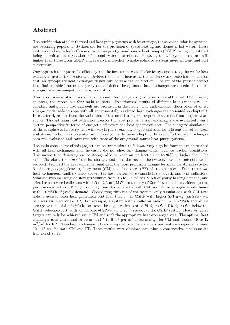
2.2.2 Ice-on-plate

Two different flat plate heat exchangers have been tested, one made of stainless steel (SS) from themanufacturer Energie Solaire and the other made of polypropylene (PP) from the manufacturer MEFA.The two flat plate types are shown in Fig. 2.5. The heat exchanger made from stainless steel have beentested with set-ups using 10, 8 and 6 units. The heat exchanger made of polypropylene was tested with10 and 8 units 3. The characteristic data of the heat exchangers is given in Table 2.2, where Hhx is theheight of the heat exchangers.

Table 2.2: Data of the flat plate heat exchangers used in the experiments.

Type nhx Lhx Hhx Ahx xhx[m] [m] [-] [m2 ] [mm]

FP-SS-10hx 10 1.854 0.834 30.9 100FP-SS-8hx 8 1.854 0.834 24.7 125FP-SS-6hx 6 1.854 0.834 18.5 167FP-PP-10hx 10 1.875 0.860 32.2 100FP-PP-8hx 8 1.875 0.860 25.8 125

(a) (b)

Figure 2.5: Picture of two flat plates experimentally evaluated made of (a) polypropylene (b) stainlesssteel.

2.3. Performance indicators

For each test sequence several indicators are calculated from measured data. The heat exchanger powerQ is calculated as:

Q = mcp(Tf,out − Tf,in) (1)

where m is the mass flow, cp the specific heat capacity and Tf the heat transfer fluid (glycol) temperature.The cumulative energy for the whole test sequence until the time t is calculated as:

Q =

∫ t

t=0

Q · dt (2)

where t is the time. The integral is discretized using a time step dt of 10 seconds. The mass ice fractionis calculated as the ratio between the mass of ice and the total amount of water and ice of the storage.

Mr =Mice

MT(3)

3Six units were not tested due to the very low performance expected from this set-up

7/60

The ice fraction is experimentally evaluated measuring the change of height of water due to the volumechange between water and ice. For some processes, e.g. melting cases where the initial ice fraction is verylarge and the ice is above water level, the mass of ice can not be accurately obtained from experimentsand therefore it is calculated from the energy exchanged between the heat exchangers and the storage,neglecting heat gains from the surroundings through the storage walls. Ice fraction results that arecalculated from the exchanged energy are labeled as M∗

r .

The global heat transfer rate of the heat exchanger UA is obtained from:

UA =Q

LMTD(4)

where the logarithmic mean temperature difference LMTD is calculated as:

LMTD =(Tf,out − Tw,av)− (Tf,in − Tw,av)

ln(Tf,out−Tw,av

Tf,in−Tw,av

) (5)

where Tw,av is the averaged water temperature in the storage. As long as ice exists in the storage, Tw,avis assumed to be 0 oC.

The heat transfer coefficient of the heat exchanger is calculated as:

U =UA

Aext(6)

where Aext is the external surface area of the specific heat exchanger analysed.

2.4. Uncertainty analyses

In the measurement procedure, there are different uncertainties that affect the confidence interval of theresults. In order to obtain a high precision, the 4-wire Pt100-temperature sensors (Class A) have beencalibrated for the temperature range of the test cycles (from -10 oC to 40 oC). Based on the calibration,the output values of each temperature sensor were corrected according to a 1st order polynomial. Theremaining uncertainty of the Pt100 sensors after calibration was in the order of 0.03-0.04 K. An electro-magnetic flow meter that has been calibrated for volume flows between 500 and 1400 l/h was used forvolume flow rate measurements. The relative uncertainty of the volume flow rate measurement after thecalibration of the flow sensor was determined to be 0.6 %. For the glycol concentration, an acceptablerange of 31.9 %-34.7 % has been defined. The maximal relative uncertainty of the mixture’s specific heatcapacity is then estimated with respect to this range and the uncertainty of the temperature measure-ment. For the analyzed experimental data it was generally smaller than 1.3%. These uncertainty valuesare used to calculate the total uncertainty of the derived values such as power or heat transfer coefficient.

The power extracted from the ice storage by the heat exchangers is calculated by:

Q = cpρV∆T = cpρV (Tout − Tin) (7)

This equation consists only of multiplications. Therefore, the uncertainty of the power can be calculatedby:

(uQ

Q

)2

=

(uV

V

)2

+

(uρ

ρ

)2

+

(ucpcp

)2

+

(u∆T

∆T

)2

(8)

The error of the cumulative energy over a testing sequence can be computed by the sum of the uncer-tainties of the power weighted with the length of the measurement time steps.

uQ2 =t∑t=0

uQ2 ·∆t (9)

The heat transfer coefficient rate (UA-Value) is calculated by Eq. 4, where Tstorage is measured also withfive Pt-100 temperature sensors. The total uncertainty of UA is then calculated by:

8/60

uUA2 =

(∂UA

∂Tout

)2

· (uTout)2 +

(∂UA

∂Tin

)2

· (uTin)2 (10)

+

(∂UA

∂Tw

)2

· (uTw)2 +

(∂UA

∂V

)2

· (uV )2

+

(∂UA

∂cp

)2

· (ucp)2 +

(∂UA

∂ρ

)2

· (uρ)2

The ice fraction is calculated from the total Volume Vtot = 2 · 1 · htot of the ice water mixture as

Mr = 100 · ρicem0· m0 − ρwVtot

ρice − ρw(11)

The variable m0 describes the total mass that was filled into the ice storage at the beginning of a testcycle. The uncertainty related to the ice fraction values is then:

uM2r =

(∂Mr

∂htot

)2

· (uhtot)2 +

(∂Mr

∂m0

)2

· (um0)2 +

(∂Mr

∂ρice

)2

· (uρice)2 (12)

The uncertainty of m0 was determined by the difference of the mass value displayed by the flow meter atthe water inlet of the ice storage and the value that has been derived from the height measurement. Theuncertainty of the ice density was estimated by computing the difference of the ice density at averagestorage temperature and at 0 ◦C. It is assumed that all the water is at 0 ◦C and therefore, ρw is notaffected by any uncertainty when ice is present.

The relative uncertainty of the extracted power is in the order of 2 %. The calculated heat transfercoefficient is affected by an uncertainty that ranges from 2.5 % up to 14 %. High uncertainty values arecaused by small temperature differences when the ice storage temperature approaches the chiller set pointtemperature and therefore the heat exchanger’s inlet and outlet temperature are close together. Thus,system operating points with significant energy transfer are not affected by large uncertainty values. Theice fraction calculation was computed based on the changing water level in the storage tank when ice isformed or melted. The ultrasonic sensor has a precision of 0.5 mm which results in an uncertainty of theicing fraction in the order of 0.5% - 1%.

2.5. Methodology

In order to test the heat exchangers an experimental sequence has been defined and programmed inLabView. The testing sequence is summarized in Table 2.3. All heat exchangers have been tested withtwo volume flows regulated with a PID control (1000 l/h and 2000 l/h). Each test lasted around oneweek for each mass flow and a total of ten heat exchanger set-ups have been evaluated.

Table 2.3: Testing sequences considered for each heat exchanger.Test phase Name Mass Flow Tset of the chiller Begin of sequence End of sequenceSensible heating S1 1000 l/h 20 oC Storage at 10 oC or end of S8 steady state

S2 2000 l/h 40 oC End of S1 steady stateSensible cooling S3 1000 l/h -10 oC End of S1 Ts,av ≈ 0 oC

S4 2000 l/h -10 oC End of S2 Ts,av ≈ 0 oCSolidification S5 1000-2000 l/h -10 oC End of S3 or S4 Vr ≈ 95% (or 3 days)Cycling : Ice/melt S6 1000-2000 l/h -10 oC (40 min)

10 oC (20 min) End of S6 10 cyclesMelting S7 1000-2000 l/h 10 oC End of S8 steady state

2.6. Experimental results

The experimental results are split into sensible heating, sensible cooling, icing, melting and cycling oficing/de-icing. Results for flat plates made of polypropylene with a volume flow of 1000 l/h are not shownin the following sections because problems with flow distribution were detected.

9/60

2.6.1 Sensible heating (S1 and S2)

The overall heat transfer coefficients (U) for sensible heating processes are shown in Fig. 2.6 . Circlemarks are for 2000 l/h and for S2, i.e. the storage is heated from 20 oC to 40 oC. Filled triangles are for1000 l/h and for S1, i.e the storage is heated from 10 oC to 20 oC.

0

50

100

150

200

250

300

U[W

/(m

2K)]

0 1 2 3 4 5 6 7 8 9 10 11 12 13 14 15

Time [h]

CM-Gtype-16hxCM-Stype-16hxCM-Gtype-8hx

CM-Stype-8hxCoil

0

50

100

150

200

250

300

U[W

/(m

2K)]

0 1 2 3 4 5 6 7 8 9 10 11 12 13 14 15

Time [h]

FP-SS-10hxFP-SS-8hxFP-SS-6hx

FP-PP-10hxFP-PP-8hx

2000 l/h 1000 l/h

(a) (b)

Figure 2.6: Overall heat transfer coefficient results for sensible heating sequences S1 and S2 for (a) ice-on-coil heat exchangers and (b) ice-on-plate heat exchangers. Circle marks are for 2000 l/h and S2 (heatingfrom 20 oC to 40 oC) and filled triangles are for 1000 l/h and S1 (heating from 10 oC to 20 oC).

FP-SS show better capabilities for providing energy to the storage by means of sensible heat. For a flowrate of 2000 l/h, U is in the range of 90-110 W/(m2K) for CM heat exchangers and between 150-200W/(m2K) for FP with SS. For 1000 l/h U values are decreased to values between 70 and 90 W/(m2K)for CM and to 100-140 W/(m2K) for FP-SS approximately. Coils shows the best performance of theice-on-coil solutions with around 100-120 W/(m2K) for 1000 l/h and 2000 l/h respectively. However, thetotal area of Coils is substantially lower than that of CM and usually low Ahx shows better performanceper m2 of heat exchanger area due to the higher temperature difference at the end of the heat exchanger.

The main difference between the two designs of capillary mats, G and S types, is the heat exchangerarea as U values are very similar. FP-PP show a much lower performance compared to FP-SS and theperformance of ice-on-coil heat exchangers is better than the one of FP-PP but worse than the one ofFP-SS. Except for FP-SS, the performance of all heat exchangers remains relatively constant during theheating process, even though the Reynolds number (Re) increases due to the lower viscosity of the fluidwhen it is heated. During the whole test sequence the Re number remains below 400 for 2000 l/h andbelow 150 for 1000 l/h and therefore it is theoretically always in a laminar regime. In a laminar flowregime the Nussels number is relatively constant and thereby the performance of the heat exchangers arenot affected by the increase of Re during the heating process and only slightly due the change of volumeflow. However, FP-SS are significantly affected by the mass flow, probably because their special designenhances turbulence. Thanks to this special design, the flow is turbulent at lower Re number as comparedto smooth pipes. Therefore, flow regimes are most of the time in the transition regime between laminarand turbulent. This means that the Nussel number and, as a consequence, the heat transfer coefficient,are affected by the Re number.

2.6.2 Sensible cooling (S3 and S4)

Overall heat transfer coefficients for the sensible cooling process are shown in Fig. 2.7. Circle marksrepresent a volume flow of 2000 l/h and a test sequence S4 in which the storage temperature is cooledfrom 40 oC to 0 oC. Triangle marks represent a volume flow of 1000 l/h and a test sequence S3 in whichthe storage temperature is cooled from 20 oC to 0 oC.

10/60

0

50

100

150

200

250

300

U[W

/(m

2K)]

0 1 2 3 4 5 6 7 8 9 10 11 12 13 14 15

Time [h]


CM-Stype-8hxCoil

0

50

100

150

200

250

300

U[W

/(m

2K)]

0 1 2 3 4 5 6 7 8 9 10 11 12 13 14 15

Time [h]


FP-PP-10hxFP-PP-8hx

2000 l/h 1000 l/h

(a) (b)

Figure 2.7: Measured overall heat transfer coefficients for sensible cooling sequences S4 for (a) ice-on-coilheat exchangers and (b) ice-on-plate heat exchangers. Solid lines are for 2000 l/h and the cycle starts atTs of 40 oC; dashed lines are for 1000 l/h and the cycle starts at Ts 20 oC.

The overall heat transfer coefficient shows a different behavior for ice-on-coil heat exchangers and FP-SS.For FP-SS, the U values decrease significantly with time. For CM the U values remain approximatelyconstant for a large time period. The reason for that is the same as given in section 2.6.1, i.e. ice-on-coilheat exchangers are always in a laminar regime while FP-SS are in the turbulent and transition regime.In this case, the Re number decreases along the sequence because the fluid’s viscosity increases whencooled down to 0 oC. At the beginning of the test sequence, FPs perform significantly better than theice-on-coil heat exchangers, and the opposite is true at the end of the test sequence. The U values rangefrom 120 to 75 W/(m2K) for 2000 l/h and from 100 to 60 W/(m2K) for 1000 l/h when ice-on-coil heatexchangers are used; and they range from 220 to 40 W/(m2K) for 2000 l/h and from 175 to 40 W/(m2K)using 1000 l/h when FP-SS are used. The evolution of U along time for FP-PP is similar to the oneobserved with ice-on-coil heat exchangers when 2000 l/h are used. The U values are relatively constantand in the range of 100 W/(m2K) for a large period. The efficiency of the heat exchangers is reducedwhen the storage water temperature is close to 0 oC.

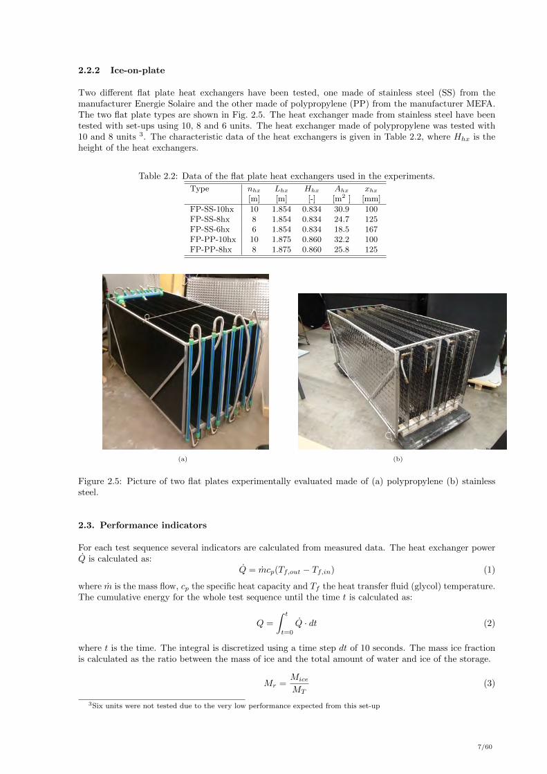
2.6.3 Solidification (S5)

The amount of ice produced for all heat exchangers are shown in Fig. 2.8. Usually, capillary mats freezethe water of the storage faster compared to flat plates. Coils have a lower rate of icing due to thelower heat exchanger area (see Table 2.1). Ice fractions of 95 % and above are achieved. Due to thespecific height of the FP used in the experiments, only 85% of the storage height was covered by theheat exchangers, limiting its capacity to ice the whole storage. However, flat plate heat exchangers canbe used to achieve very high ice fractions (above 95%). Mass ice fractions higher than 85% with FPare possible. However, above 85 %, the U value is very low since ice has to grow on the surface of acompact ice cube that includes all plates and thus, the path between the heat transfer fluid in the heatexchanger and liquid storage water is long. For FP, ice fractions above 90% where achieved. During theicing experiments and also at the maximum ice fractions up to 100% no damaging of the casing could beobserved with any of the heat exchangers used.

The overall heat transfer coefficient is shown in Fig. 2.9 as a function of the ice fraction. The referencearea for the calculation of the heat transfer coefficient is the external heat exchanger area, as in all theother cases. From this graph, it can be observed that the decrease of U for ice-on-coil heat exchangersis much smaller compared to FP. Considering the ideal case of ice growing on a single tube, the higherthermal resistance of the ice layer when ice grows is partially compensated by the higher contact areabetween the outside of the growing ice radius and the surrounding water. Therefore, the heat transferrate UA remains relatively constant when ice grows on a cylinder (Carbonell et al., 2015). However, ice-

11/60

0

10

20

30

40

50

60

70

80

90

100

Vr

0 10 20 30 40 50 60 70 80 90 100

Time [h]


CM-Stype-8hxCoil

0

10

20

30

40

50

60

70

80

90

100

Vr

0 10 20 30 40 50 60 70 80 90 100

Time [h]


FP-PP-10hxFP-PP-8hx

2000 l/h 1000 l/h

(a) (b)

Figure 2.8: Evolution of mass ice fraction over time for the icing sequence S5 for (a) ice-on-coil heatexchangers and (b) ice-on-plate heat exchangers.

0

50

100

150

200

250

U[W

/(m

2K)]

0 10 20 30 40 50 60 70 80 90 100

Vr


CM-Stype-8hxCoil

0

50

100

150

200

250

U[W

/(m

2K)]

0 10 20 30 40 50 60 70 80 90 100

Vr


FP-PP-10hxFP-PP-8hx

2000 l/h 1000 l/h

(a) (b)

Figure 2.9: Measured overall heat transfer coefficients as a function of the ice fraction for the icingsequence T5 for (a) ice-on-coil heat exchangers and (b) ice-on-plate heat exchangers.

on-coil heat exchangers are composed of many tubes and the ideal one-dimensional growing on a singletube is only valid until growing of ice from neighboring tubes contact with each other. For example,for the S-type, the distance between tubes in one heat exchanger is 20 mm. Assuming that ice growshomogeneously on all pipes and along the whole pipe length, ice layers start to touch to each other withinone heat exchanger when Vr is approximately 27% and 14% for 16 hx and 8 hx respectively. For G-type,the distance between pipes is 30 mm, this means that ice layers between pipes touch when the ice fractionis approximately 80% and 40% for 16 hx and 8 hx, respectively.

The consequences of physical contact between ice layers is usually called constrained ice growing (Jekelet al., 1993). For all CM, the heat exchangers undergo of a two step constrained ice growing, the first onewhen the ice is constrained within one heat exchanger (ice between adjacent tubes touch each other) andthe second when ice is constrained between neighboring heat exchangers. When ice growing is constrainedthe overall heat transfer coefficient decreases compared to the unconstrained case because the contactarea between the growing ice and surrounding storage water decreases. However, in the experimentalresults it is not possible to observe a sharp decrease of the U value when ice constrainment occurs becauseice grows unequally along the length of each tube and thus the constrainment of ice growth starts at the

12/60

cold inlet and progresses slowly towards the end over a long period.

For FP, ice starts to be constrained when the ice thickness is half the distance between heat exchangers.In the experiments shown here, this corresponds always to an ice fraction of approximately 83%. Atthese conditions all water between heat exchangers is frozen and ice can only grow on the surface of asolid cube of ice with very low U values. Comparing all heat exchangers one can observe that for low icefractions the U values of FP-SS are higher. However, the decrease of the U value when ice grows is muchmore pronounced for FP-SS compared to ice-on-coil heat exchangers. As stated before, the contact areabetween ice and water increases when ice grows in ice-on-coil heat exchangers. Instead, for FPs the icesurface area remains approximately constant and the U value decreases rapidly. For FP with PP, thedecrease of efficiency is much less pronounced in comparison to SS because the heat transfer resistanceof the polypropylene is the limiting factor, in comparison to the FP-SS, where the ice thickness is thelimiting factor.

2.6.4 Melting (S9)

The energy delivered for melting the ice is shown in Fig. 2.10. Melting 2 m3 of water needs about 185kWh. On top of that, the energy needed to heat the sub-cooled ice to 0 oC and the sensible heat to raisethe temperature from 0 oC to 10 oC needs to be considered. Comparing CM with FP one can observe

0

25

50

75

100

125

150

175

200

Q[kW

h]

0 10 20 30 40 50

Time [h]


CM-Stype-8hxCoil

0

25

50

75

100

125

150

175

200

Q[kW

h]

0 10 20 30 40 50

Time [h]


FP-PP-10hxFP-PP-8hx

2000 l/h 1000 l/h

(a) (b)

Figure 2.10: Energy delivered to the storage by the heat exchangers for the melting sequence S9 for (a)ice-on-coil heat exchangers and (b) ice-on-plate heat exchangers.

that FP-SS are usually able to melt completely the ice in less time. The measure for the ice fraction forcapillary mats was not accurate with the method used in these experiments. A water layer above the iceblock was not always present at high ice fraction (≥ 95%) and the measurement of solid ice was disturbingthe accuracy. Because the flat plates had a layer of 17 cm of water above them, the measurement of themelted ice was much more accurate. However, even in this case, with the method used, it is not possibleto measure the ice fraction until the melted ice connects with the water of the storage. Ice is meltedaround the heat exchangers forming a cavity of liquid water. Before this cavity of melted ice connects tothe bulk water, the change of density when the ice is melted creates an under-pressure around the heatexchangers that would either expand the heat exchanger or evaporate part of the water until the changeof volume is filled.

Overall heat transfer coefficients are shown in Fig. 2.11. FP-SS have the highest melting capacity athigh ice fractions with values above 250 W/(m2K). For ice fractions below 60% the U values reduce to50-60 W/(m2K) for FP-SS. For ice-on-coil heat exchangers, the U values are more stable over the wholemelting process with values between 50-80 W/(m2K).

13/60

0

50

100

150

200

250

300

U[W

/(m

2K)]

0 10 20 30 40 50 60 70 80 90 100

V ∗r


CM-Stype-8hxCoil

0

50

100

150

200

250

300

U[W

/(m

2K)]

0 10 20 30 40 50 60 70 80 90 100

V ∗r


FP-PP-10hxFP-PP-8hx

2000 l/h 1000 l/h

(a) (b)

Figure 2.11: Overall heat transfer coefficient for melting sequence S9 for (a) CM and (b) FPs.

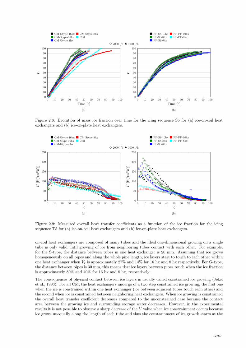
2.6.5 Cycling (S8)

The cycling experiment consist of 10 sequences of heating and cooling which are used for melting andicing. This test sequence is performed at a very high ice fraction after the icing sequence S5. Eachcycle is performed with a constant time of 20 min for heating and 40 min for cooling. All experimentswith CM were tested with cycles always in the subcooled zone (ice temperature was below 0 oC) andtherefore melting was not always achieved. For this reason the test control was changed such that itheats up the storage until the outlet of the heat exchanger is close to zero before cycling starts. In thisway it is ensured that ice is melted and solidified during each cycle. As an example, results for cyclingsequences are presented in Fig. 2.12 for FP with 10 hx. For all the cycles the inlet temperature of theheat exchangers increases above 0 oC, which means that it is always possible to melt ice, at least at theentrance of the heat exchangers. For the first four cycles, the outlet temperature remains at 0 oC, whichmeans that ice is never subcooled at the end of the heat exchanger. After the first cycles, the outlettemperature starts to drop below 0 oC which means that ice is subcooled, and the UA values are reducedbecause the heat of fusion is not released along the whole length of the hx.

The danger of breaking the casing of the storage is potentially higher when cycles of melting and icing areperformed at high ice fractions. In normal icing conditions without any cycles, the solid ice will alwayspush the liquid water to the surface. Therefore, as long as there is an escape way for the water, thereis no risk for the casing. The problem may occur when a volume of water in contact with the casing istrapped within an ice block. If then this water is iced, the volume expansion will produce a strong forceto the wall of the casing with the danger of breaking it. This situation may occur when the dynamics ofthe system are on a specific state, which however was never the case in the lab.

In this test several cycles of melting and icing have been performed at very high ice fractions in orderto test the robustness of the heat exchangers under these dynamic conditions. The mechanical stressthat was caused by the dynamics of icing and melting was neither found to be a problem for the heatexchangers nor for the storage casing. However, long term tests should be performed to investigate therobustness and stability.

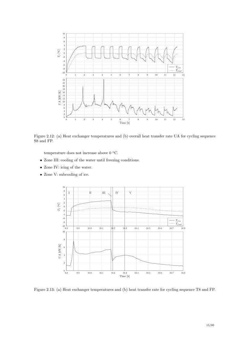
The cycling sequence will also be very useful for the validation of the ice storage model (see chapter 4),since in each cycle different physical phenomena take place. Fig. 2.13 shows one cycle of melting andicing for FP-SS with 10 hx (zoom into Fig. 2.12). The sequence has been split into five zones, from I toV as shown in Fig. 2.13. Zones I to II correspond to heating/melting and zones III to V correspond tocooling/icing.

• Zone I : switch from cooling to heating.

• Zone II: the ice is heated from the subcooled state to 0 oC and melted starting from the entranceof the heat exchangers. Most likely, melting does not occur over the whole length since the outlet

14/60

-10

-8

-6

-4

-2

0

2

4

6

8

10

Tf[oC]

0 1 2 3 4 5 6 7 8 9 10 11 12 13

Tf,in

Tf,out

0

2

4

6

8

10

12

14

16

18

20

22

24

UA

[kW

/K]

0 1 2 3 4 5 6 7 8 9 10 11 12 13

Time [h]

Figure 2.12: (a) Heat exchanger temperatures and (b) overall heat transfer rate UA for cycling sequenceS8 and FP.

temperature does not increase above 0 oC.

• Zone III: cooling of the water until freezing conditions.

• Zone IV: icing of the water.

• Zone V: subcooling of ice.

-10

-8

-6

-4

-2

0

2

4

6

8

10

Tf[oC]

9.8 9.9 10.0 10.1 10.2 10.3 10.4 10.5 10.6 10.7 10.8

Tf,in

Tf,out

0

2

4

6

8

10

UA

[kW

/K]

9.8 9.9 10.0 10.1 10.2 10.3 10.4 10.5 10.6 10.7 10.8

Time [h]

I II III IV V

Figure 2.13: (a) Heat exchanger temperatures and (b) heat transfer rate for cycling sequence T8 and FP.

15/60

2.7. Conclusions

In the present chapter results of several heat exchangers have been analyzed, including capillary matswith different designs made of polypropylene, polypropylene coils and flat plates made of stainless steeland polypropylene. The area analyzed has been modified for each heat exchanger and all test havebeen performed using two different mass flow rates. In total, nine possibilities have been experimentallyevaluated for several test sequences including sensible heating and cooling, icing, melting and cycling.The main conclusions of this experimental study can be summarized as:

• Very high ice fraction can be reached with all heat exchangers and mass flows.

• The casing did not show any damage under high ice fraction conditions. This means that designingan ice storages able to reach 95% ice fraction or higher should be safe.

• All heat exchangers showed to be reliable and robust under the test conditions. Long term testswere not carried out.

• Flat plates made of stainless steel are better suited compared to capillary mats or coils for sensibleheating and cooling and for melting processes.

• Capillary mats or coils are better suited compared to flat plates for the icing process due to thestrong decrease of performance that flat plates suffer when ice grows.

• Flat plates made of polypropylene have shown the worst thermal performance of all tested heatexchangers.

• Coil heat exchangers made of polypropylene for small ice storages were difficult to design and build.Therefore, it does not seem to be the a promising solution for low ice storage volume (< 5 m3).

3. Mathematical modelling of the ice storage

In this chapter, an ice storage model able to use capillary mats, coils and flat plate heat exchangers isdescribed.

3.1. Literature review on ice storage models

Ice storage concepts can be classified as direct or indirect. In direct concepts, the heat exchanger is usedto solidify water around the heat exchanger, while melting takes place by circulating warm water throughthe storage without any heat exchanger. Therefore, the ice is melted on the outside surface of the icelayer. Indirect concepts are those in which both solidification and melting is possible due the circulationof a brine solution in the heat exchanger. Since ice is melted on the surface of the heat exchanger indirectconcepts are sometimes called internal melting concepts. The model presented in this paper, and thusthe literature review described hereafter, is only focused on the indirect approach.

Phase change processes can be modeled at different levels of complexity, from empirical models to Com-putational Fluid Dynamics (CFD). In order to be able to assess the feasibility of an ice storage concept forsolar heating applications yearly dynamic simulations are required. Therefore, complex models that needhigh computational time are not appropriate for this application. Many ice storage models have beendeveloped until today. Most of the ice storage models can be classified into storage or heat exchangerbased models. Storage models are focusing on the conservation of energy of the storage water, while heatexchanger based models are looking at the problem from the heat exchanger perspective. The secondapproach is usually profiting from the fact that water temperature in the storage remains close to 0 oCwhile ice exists and, thus, the storage model is simplified to an energetic balance in one control volume.

Jekel et al. (1993) developed a model based on the energy balance in the storage and heat transfer rateequations for heat exchanger predictions. The heat exchangers were modeled using a logarithmic meantemperature difference approach assuming a constant overall heat transfer coefficient from brine to bulkwater along the heat exchanger length. Only one control volume was assumed for the water storage aswell as for the heat exchanger. The solidification and melting was based on horizontal, spiral woundtubes spaced on a square grid. The process of extracting the sensible and latent heat from water was

16/60

split into sensible, unconstrained and constrained solidification and melting (see section 3.2.5 for furtherdetails). Averaged differences between simulations and manufacturers data were found to be up to 10%for the melting process. Because only manufacturers data was used, the validation of the model is lackingdocumented comparisons with experimental data. The main limitations of this model are that i) it isnot valid for partial icing and melting and thus not able to predict correctly cycles of icing and melting;ii) only one control volume was assumed in both heat exchanger and storage iii) ice constrainment wasconsidered assuming only symmetric cases and iv) the sensible heat in the ice was neglected (ice wasassumed to be always at 0 oC).

Drees and Braun (1995) used the model developed by Jekel et al. (1993) and improved it by usingdiscretization techniques in the the heat exchanger and by using more appropriate equations for forcedconvection inside a spiral tube geometry. Validation was provided with experiments with differences upto 6% for the energy exchanged in the melting period.

Vick et al. (1996) developed a model in which partial charge and discharge was considered by taking intoaccount the possible existence of several and alternate layers of water and ice due to partial melting andicing. The creation of multiple layers made the model more complex. As a difference from the modelscited above, two tubes were simulated to consider a counterflow arrangement. Moreover, the thermalcapacity of ice, brine and tube walls was considered. As in the model of Drees and Braun (1995) theheat exchanger is discretized along the fluid flow path. The model was compared with experimental datain Nelson et al. (1996) with satisfactory results, but without quantifying differences between simulationsand experiments. The main disadvantage of this model is that ice constrainment is not considered, whichis a key aspect when high ice fractions are reached.

Neto and Krarti (1997a) presented a model where constrained ice growing was considered using a regularsquare geometry of tubes but considering different ice diameters on the tubes. The latter model wasvalidated in Neto and Krarti (1997b) and the authors reported differences of 5% for energy exchanged atthe end of the analyzed process. The model from Neto and Krarti (1997a) is the most detailed from thementioned above. However, due to their consideration of the geometry of the coils in a detailed manner,the extension to other heat exchanger designs would be difficult. Moreover, the model is using an analyticsolution for ice constrainment which is only valid for a symmetric case. As will be shown in section 4,the consideration of asymmetric cases is of relevance if capillary mats are to be modeled.

Koller et al. (2012) developed a model with similar features than those provided by Jekel et al. (1993), butnatural convection around the tubes during the melting process of the water was considered. Comparisonswith experimental results were provided with differences up to 10 % for the energy injected into the storagein the melting phase.

Most of the above mentioned models are focusing on the solidification and melting of ice around theheat exchangers and thus the modeling of the storage is highly simplified. Therefore, these models arevalid if the temperature of the water remains close to 0 oC. For solar heating applications, the storageis used as cold source in winter and as heat sink in spring, summer and beginning of autumn. Thus,numerical models need to consider several control volumes along the height of the storage, consideringthe heat conduction between water layers, losses and gains from the ambient, and the density gradientsof water that lead to stratification of the storage tank. Validations of the models for sensible heatingand cooling of the storage water is also not usually reported in the literature. In the work presented byCarbonell et al. (2016c, 2015) those phenomena were considered. However, the ice storage concept inthese publications was based on flat plate heat exchangers with thermal de-icing and therefore maximumice thickness on the heat exchangers were low. Validation with different numbers of heat exchangers wasnot carried out in any of the cited articles. Thus, the model performance for other configurations thanthe reported ones, e.g. different heat exchanger spacing, is unknown.

The model presented in this paper considers ice constrainment for both symmetric and asymmetric cases,where different distances between pipes or heat exchangers can be defined along the width and the lengthof the storage. This feature is necessary if different numbers of heat exchanger units in the ice storageand thus different spacing between tubes shall be analyzed. Another important feature of this paper isthat the number of experiments carried out is large, including two heat exchanger designs with differentnumber of capillary mat units, four testing sequences (sensible heating, sensible cooling, solidification andmelting) with two different volume flows (2000 l/h and 1000 l/h). The validation carried out is way moredetailed, and therefore more challenging, compared to most of the publications found in the literature.

17/60

3.2. Mathematical formulation

The formulation of the ice storage model is based on the solution of the energy conservation law appliedto the water of the storage Carbonell et al. (2015):

ρcp∂T

∂t+ (ρcp)ice

∂Tice∂t

=∂

∂y(λ∂T

∂y) +

hfV

∂Mice

∂t+ qsurr + qhx (13)

where cp is the specific heat capacity of water, hf the enthalpy of fusion, Mice the mass of ice, qextand qhx are the heat fluxes per unit volume between the storage fluid and the surroundings and heatexchanger respectively, T the water temperature, t the time, V the water volume of the storage, y thecoordinate along the height of the storage, λ and ρ are the heat conductivity and density of water. Thefirst and second term of Eq. 13 represents the accumulated sensible heat of the fluid and solid ice. Thefirst term of the right side of Eq. 13 is the heat of conduction between control volumes and it is calculatedusing the conductivity of water at the specific temperature multiplied by the effective conductivity factorλeff = λw(T ) · reff . The latter is used in order to account for conduction in the walls of the storage.The second term of the right hand side of Eq. 13 represents the latent heat of solification and meltingand the last term two terms are the heat provided by the surroundings and heat exchangers respectively.

A drawback of this formulation is that the model is not able to handle a 100 % ice fraction in any controlvolume, since the energy balance is done in the liquid phase. When the water volume is extremely low,the stability of the model is penalised since any heat gains/losses means high temperatures changes inone time step.

3.2.1 Heat from/to the surroundings

The third term of the right side of Eq. 13 represents the heat losses to the surroundings through theexternal surface area of the storage tank Aext. It is calculated assuming a constant heat transfer coefficientUext for each control volume j as:

Qext,j = Uext,jAext,j(Tj − Text,j) (14)

where Qext,j = qext,jV and Text is the temperature of the surroundings, which in the present case can bethe ground or cellar temperature depending on the placement of the storage. The heat loss coefficient isprovided as an input of the model for several surfaces, i.e. top, bottom and lateral sides. The latter issplit into two values, one for the upper and one for the lower half of the lateral sides.

3.2.2 Heat exchangers

The heat exchanger is solved by a step-by-step model, which consists of a one-dimensional analysis inthe fluid direction applying a finite control volume discretization technique. The energy balance insidethe circulating fluid takes into an account the thermal losses through the external surface and convectiveheat transfer with the neighboring control volumes neglecting the axial heat conduction.

The discretized mesh is displaced (the node is at the fact of the CV) for m, T and P , but is centered(the node is at the centre of the CV) for the storage water Tw and wall Twall temperatures. Applyingthe mass conservation law in the whole domain, the mass flow rate at the outlet is directly obtained fromthe given mass flow rate at the inlet:

mout = min (15)

Under the above mentioned hypothesis, the energy conservation expression is discretized resulting in analgebraic equation in terms of temperature for a CV i of the form:

(ρcpV )iTi − Ti

0

∆t+ mcp,i(Ti+1 − Ti) = (UA)i

(Tw,i − Ti

)(16)

The subscripts i and i + 1 represents the value at the inlet and outlet of the CV i respectively and thesuperscript 0 refers to the value at previous time step. The UA is the overall heat transfer rate coefficient

18/60

from the fluid to the bulk storage water Tw, T represents the arithmetic average of the temperaturebetween the temperatures at the faces of the CV i and i+1. The overall heat transfer coefficient iscalculated as explained in section 3.2.3.

Algebraic equations resulting from the discretized energy and mass conservation laws shown above aresolved from inlet to outlet following a step-by-step procedure (from CV i to the next CV i+1). The modelneeds no iterations if UA is known and the thermo-physical properties are calculated from conditionsat the inlet of the CV. From the mass flow rate and temperature of the fluid at the inlet, and properboundary conditions, the distribution of temperatures, mass flow rate (constant), and heat losses or gainsthroughout the physical domain are calculated.

3.2.3 Overall heat transfer coefficient

The main task in solving the heat exchanger is to calculate the overall heat transfer coefficient UA fromEq. 16. For situations where solidification/melting takes place, the UA reads:

UA =1

1αinAin

+ 1UAwall

+ 1UAice

+ 1αoutAout

(17)

where the subscripts in, wall, ice, and out refer the internal fluid, wall, solidification and melting ofice and outside heat transfer coefficients. The αin and αout need to be defined for different boundaryconditions and heat exchanger types. A summary of Equations used for those cases are shown in Table3.1.

For tubes, the total heat transfer coefficient is obtained as:

UA =1

1Aiαi

+ln

dp,outdp,in

2πLhxλp+

lndice

dp,out

(2π−φcons)Lhxλice+ 1

Aiceαo

(18)

where dp is the pipe diameter, Lhx is the length of the pipe and φcons is the overlapping contact areabetween growing ice due to ice constrainment (see section 3.2.5 for more details). Therefore, the usefulheat exchange area where ice and water are in contact is reduced by the overlapping as:

Au = (2π − φcons

2)diceLhx (19)

The heat transfer coefficient per useful area Au is obtained from:

U =1

(2π−θcons)2π

(dice

dp,inαin+ dice

dp,outαo+

dicelndp,outdp,in

2λp

)+

dicelndice

dp,out

2λice

(20)

All results presented in this report are based on a U value per external heat exchanger area as presentedin Eq. 6. However, for the calculation of the model Eq. 20 is used.

3.2.4 Ice solidification and melting on the heat exchanger

The term for heat of solidification and melting appearing in Eq. 13 is defined as:

Qlat = hf∂Mice

∂t= hfρice

∂Vice∂t

(21)

Assuming a small time step, the latent heat due to ice growing on a cylinder tube surface can be linealizedas:

Qlat = hfρiceπL(rice)

2 − (r0ice)

2

∆t≈ hfρice2πLr0

ice

rice − r0ice

∆t(22)

where r0ice is the radius of the previous time step. Rearranging Eq. 22, the radius for the new time step

rice can be obtained:

rice =Qlat∆t

hfρice2πLr0ice

+ r0ice (23)

19/60

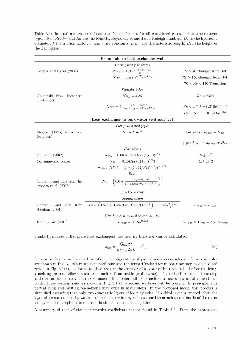
Table 3.1: Internal and external heat transfer coefficients for all considered cases and heat exchangertypes. Nu, Re, Pr and Ra are the Nusselt, Reynolds, Prandtl and Raleigh numbers, Dh is the hydraulicdiameter, f the friction factor, C and n are constants, Lchar the characteristic length, Hhx the height ofthe flat plates

Brine fluid to heat exchanger wall

Corrugated flat plates

Cooper and Usher (2002) NuL = 1.68(RePrDhw

)0.4 Re ≤ 70 changed from Ref.

NuT = 0.2(Re0.67Pr0.4) Re ≥ 150 changed from Ref.

70 < Re < 150 Transition

Straight tubes

Gnielinski from Incroperaet al. (2006)

NuL = 4.36 Re < 2300

NuT = f8

(Re−1000)Pr

1+(12.7(f/8)0.5(Pr2/3−1)Re < 2e4 f = 0.316Re−0.25

Re ≥ 2e4 f = 0.184Re−0.2

Heat exchanger to bulk water (without ice)

Flat plates and pipes

Morgan (1975) (developedfor pipes)

Nu = CRan flat plates Lchar = Hhx

pipes Lchar = dp,out or Hhx

Flat plates

Churchill (2002) NuL = 0.68 + 0.67(Ra · f(Pr))1/4 Ra≤ 1e9

(for immersed plates) NuT = 0.15(Ra · f(Pr))1/3) Ra≥ 1e12

where f(Pr) = (1 + (0.492/Pr)9/16))−16/9

Tubes

Churchill and Chu from In-cropera et al. (2006)

Nu =

(0.6 + 0.387Ra1/6

(1+(0.559/Pr)9/16)8/27

)2

Ice to water

Solidification

Churchill and Chu fromStephan (2006)

Nu =(

0.825 + 0.387 [Gr · Pr · f(Pr)]16

)2

+ 0.435Lchar2rE

Lchar = Ltube

Gap between melted water and ice

Koller et al. (2012) Nugap = 0.3Ra0.238 Nugap > 1 λw = λw ·Nugap

Similarly, in case of flat plate heat exchangers, the new ice thickness can be calculated:

sice =Qlat∆t

hfρice2πL+ s0

ice (24)

Ice can be formed and melted in different configurations if partial icing is considered. Some examplesare shown in Fig. 3.1 where ice is colored blue and the formed/melted ice in one time step as dashed redzone. In Fig. 3.1(a), ice forms (dashed red) at the exterior of a block of ice (in blue). If after the icing,a melting process follows, then ice is melted from inside (white zone). The melted ice in one time stepis shown in dashed red. Let’s now imagine that before all ice is melted, a new sequence of icing starts.Under these assumptions, as shown in Fig. 3.1(c), a second ice layer will be present. In principle, thispartial icing and melting phenomena may exist in many steps. In the proposed model this process issimplified assuming that only two concentric layers of ice may exist. If a third layer is created, then thelayer of ice surrounded by water, inside the outer ice layer, is assumed to attach to the inside of the outerice layer. This simplification is used both for tubes and flat plates.

A summary of each of the heat transfer coefficients can be found in Table 3.2. From the expressions

20/60

r,o

r,ice

dr,ice

(a)

r,o

r,melt

r,ice

(b)

Ice Water

r,o

r,ice,out

Glycol r,meltIce

r,ice,in

(c)

Figure 3.1: (a) Ice growing on a cylinder and (b) ice internal melting (c) partial icing and melting.

shown in this Table, the UA value for flat plates can also be derived.

Table 3.2: Equations for flat plates and cylinder heat exchangers.

Equation Flat plate Cylinder

αi, αo see Table 3.1 Table 3.1

UAwall Ahxλwallδwall

2πLλwallln(dout/din)

UAice Ahxλicesice

2πLλicefconsln(dice/dout)

3.2.5 Constrained calculation

When ice grows on a circular tube and the radius of icing is larger than half the distance to the nexttube, the two ice surfaces are in contact, which leads to a decreased surface of the ice-to-water contactarea and thus to a decreased heat transfer capacity. In a first approximation, it is useful to treat theproblem purely geometrically. The total area of constrained surface Acons, where the heat transfer isnegligible because of symmetry, can be described by the overlapping angle of the cylinder φcons and theicing radius:

Acons = rice · φcons · Ltubes (25)

where Ltubes is the length of the tube. Assuming a symmetric case, where all tubes are parallel (sameflow) and equally distant from each other, the center of the tubes form a quadratic grid. The solutionfor the overlapping angle in this case was proposed by Neto and Krarti (1997b):

φcons = 8 · ntube,tot · cos−1

[x

rice

](26)

where x is half the distance between tubes. The present model needs to consider a grid with differentdistances in the two axis. Therefore, the longer and the smaller grid distances are considered, namelyxlarge and xsmall respectively. Figure 3.2 shows the considered grid where xlarge represents half thedistance between tubes in the x-axis and xsmall represents half the distance between tubes in the y-axis.The critical radius of the ice cylinder where the surface area is constrained is rice > xlarge and rice > xsmallrespectively. When neglecting the outermost tubes that are not surrounded by four neighboring tubes,the angle related to the total surface can be calculated as:

φcons = 2 · φsmall + 2 · φlarge = 4 · ntube,x · cos−1

[xlargerice

]+ 4 · ntube,y · cos−1

[xsmallrice

](27)

where ntube,x and ntube,y are the number of tubes in the two directions of the grid. Notice that Eq. 26 isa particular case of Eq. 27 where xsmall = xlarge = x.

The total active area can then be calculated from the total area as:

Aactive = 2πrice · ntube,x · ntube,y − φcons · rice = Auncons

(1− φcons

2π

)(28)

21/60

Figure 3.2: Schematic drawing of the geometry used in the constraint ice calculation.

From this equation a surface correction factor Ar can be defined as:

Ar =

(1− φcons

2π

)= 1−

(2cos−1(

xlarge

rice)

π

)−(

2cos−1(xsmall

rice)

π

)(29)

A model based on Eq. 27 assumes that the heat flux exchanged when ice growing is constrained isproportional to the surface area between ice and water. However, since the temperature gradient andthe heat flux will not be radial in the constraint case the conductance is not proportional to the activesurface. Based on the ideas above, a correction factor of the conductance can be defined based on thesurface correction factor Ar as:

fcons(Ar) =Qcon

Qunc(30)

where Qunc is the ideal (unconstrained) heat flux through a cylindrical annulus with inner radius rpipe and

outer radius rice and Qcons is the real (constrained) heat flux. The factors fcons and Ar were originallydefined in Jekel et al. (1993) and correlated under the assumption that the ice cylinder is connectedat four alternate equidistant points along the surface perimeter. In that symmetric case, the surfacecorrection factor reduces to:

Ar = 1−(

4cos−1( xrice

)

π

)(31)

where x is the distance between equidistant tubes. In Jekel et al. (1993), a correction function was fittedto heat flux values that were calculated using a finite element calculation.

fjekel = −1.441 ·Ar + 2.455√Ar +

(3.116 ·Ar − 3.158

√Ar) rice,ideal

xsmall(32)

The correction factor can also be obtained from the constrained angle from Eq. 27 considering only thegeometry as:

fφcons= 1− φcons

2π(33)

Notice that this correction factor is exactly equal to the argument Ar defined in Eq. 29 which is used tocalculate fjekel. Therefore, the use of the correction factor fjekel, can be considered as an extension ofthe geometrical factor.

22/60

Figure 3.3: Geometry where ice is constrained in (a) the xsmall axis and (b) in both axis. The rice,idealis defined as the unconstrained radius that leads to the same area (blue zone) as the constrained area

The method proposed by Jekel et al. (1993) has been further extended in the present project in orderto consider different distances between tubes in the x and y direction of a rectangular grid. A modifiedcorrection factor fcons was derived using the FEM solver of ANSYS CFX. A 2D model of a constrainedice piece was build in the shape of the constrained ice geometry shown in Fig. 3.3. The figure on the lefthand side shows the case in which constrainment only happens in the direction of xsmall. The right figureshows the case in which the icing surface is constrained in all directions. All surfaces except Aactive andthe pipe surface are adiabatic due to the symmetry of the heat exchanger arrays. The heat flux valueswere calculated in ANSYS keeping the pipe surface at -4 oC and the active outer surface at 0 oC. Theresulting correction factor of the heat flux through the surface f(Ar, α, β) is related to the ratios:

α =xsmall

min(rice, xlarge), α ∈ (β, 1] (34a)

β =rpipe

min(rice, xlarge), β ∈ (0, 1) (34b)

The function f(Ar, α, β) was evaluated on a grid of total 1100 points. The grid contains values of α in therange of 0.16 < α < 1 and values of β range of 0.064 < β < 0.25. In order to implement the correctionfactor function f(Ar, α, β) into the simulation model, a fitting function was derived:

fcons(Ar, α, β) = Arw1Ar2+w2β

2+w3α2+w4Arβ+w5Arα+w6βα+w7Ar+w8β+w9α+w10 (35)

The function used fulfills the requirements fcons(0, α, β) = 0 and fcons(1, α, β) = 1 for all α and β. Thefree parameters of the function have been fitted to the FEM-results using a least squares algorithm. Theresulting values of the fitting are given in Table 3.3. The fitting function resulted in an absolute RMSerror of 0.018 at the evaluated points.

The used model always assumes that ice grows ideally as a perfect cylinder. The area using the the idealradius rice,ideal and the real rice differ depending on the amount of overlapping area. Starting from thetotal ice area it is straight forward to calculate the radius rice,ideal of circular tubes around the heatexchanger (filled area in Figure 3.3) that leads to the same area (same ice volume when consideringthe length). However, for the fitting function, the radius of the assumed constrained ice surface riceis necessary. There is no analytic solution to the geometric equation that relates rice,ideal and rice.Therefore, another fitting function g(γ, α, β) is used such that the following equation holds:

rice = g(γ, α, β) · rice,ideal (36)

The used fitting function is again a quadratic function in three variables:

g(γ, αg, βg) = v1γ2 + v2α

2g + v3β

2g + v4γαg + v5γβg + v6αgβg + v7γ + v8αg + v9βg + v10 (37)

23/60

Where the coefficient γ is defined as:

γ =rice,idealrsmall

(38)

In Eq. 37, a modified version of α and β, namely αg and βg, are used:

αg =xsmallxlarge

(39a)

βg =rpipexlarge

(39b)

The above equations are not exactly the sames as the ones defined in Eq. 34a and Eq. 34b because thereal rice is not know before hand. Therefore, it is not possible to know if the ice will be constrained inthe xlarge axis.

All the above definitions ensure that the following applies:

0 ≤ rice < xsmall → Ar = 1, α = 1, β = 1→ fcons(1, 1, 1) = 1 (40)

Table 3.3: Best fit values of the generalized correction function f(Ar, α, β)

Coefficient Fitting value Coefficient Fitting value

w1 0.18142704 v1 -0.24882159w2 0.12806988 v2 3.21603436w3 0.59817959 v3 -0.36384021w4 0.38678919 v4 1.98830385w5 -1.63787425 v5 0.38896584w6 -0.47262632 v6 0.53800171w7 1.43174888 v7 2.14297332w8 0.79350135 v8 -3.20396299w9 -0.80224704 v9 1.41740863w10 0.41533001 v10 -2.38774657

The function was fitted to the calculated values that have been extracted from the ANSYS model. Thebest fit parameters are shown in Table 3.3. The absolute RMS of the fit function of g(γ, αg, βg) is 0.025.For a given heat exchanger geometry the correction value can be approximated in the following way:

rice = max(1, g(γ, α, β)) · rice,ideal (41)

The max function introduces a lower bound to the fitting function g(γ, α, β) which improves the result.Values below 1 are nonphysical due to rice > rice,idel. However, they can result as an artifact of fittinginaccuracy.

3.2.6 Comparison between ice constrainment models

A comparison between the results of the different constrainment methods explained in section 3.2.5 isshown in Fig. 3.4. The graphs show the correction factor f according to the methods described in Eq. 32and Eq. 33 and in the present work (fconst). In order to apply Eq. 32 on a non-symmetric case, theaverage distance between xsmall and xlarge is used as x.

When rice/xsmall reaches 1 then the ice is constrained in the xsmall axis. In the second y-axis theratio rice/xlarge is presented. When rice/xlarge reached 1, then ice is constrained in both directions. Thisphenomena can only be considered by the present model fcons, the others can not deal with constrainmentin two directions. As can be observed in Fig. 3.4, there are large differences between the methods, whichare mainly due to different range of validity and different definitions of rice. The larger the asymmetrybetween tubes, the stepper the decrease of fcons, and thus power, when the ice is constrained in twoaxis. The most asymmetric case is Stype-8hx, where the distance between tubes in the heat exchangeris 20 mm and the distance between tubes of different heat exchangers is 120 mm. For this case, whenrice/xlarge is equal to 1 the fcons decay to zero rapidly, while in the Gtype-16hx (the symmetric case) thedecay is slower. The correction function fjekel is only valid for the symmetric case Gtype-16Hx. Both

24/60

fconst and fjekel take into account the difference between rice,ideal and rice and therefore decay to zeroat the same value in the symmetric case. The geometric function fφcons

can be used for the rectangulargrid as well but it is completely based on rice,ideal. Thus, the correction factor has non-negative valuesfor large radius rice where in reality everything would be fully iced.

0.0

0.2

0.4

0.6

0.8

1.0

f con

s

0.0

0.5

1.0

1.5

2.0

2.5

0.0 0.5 1.0 1.5 2.0 2.5 3.0 3.5 4.0 4.5

rice/xsmall

Gtype-8Hx

0.0

0.2

0.4

0.6

0.8

1.0

0.0

0.5

1.0

1.5

2.0

2.5

r ice/x

l arge

0.0 0.5 1.0 1.5 2.0

rice/xsmall

Gtype-16Hx

0.0

0.2

0.4

0.6

0.8

1.0

f con

s

0.0

0.5

1.0

1.5

2.0

2.5

0 2 4 6 8 10 12 14

rice/xsmall

Stype-8Hx

0.0

0.2

0.4

0.6

0.8

1.0

0.0

0.5

1.0

1.5

2.0

2.5

r ice/x

l arge

0 1 2 3 4 5 6 7

rice/xsmall

Stype-16Hx

(a) (b)

(c) (d)

fcons fjekel fφcons

Figure 3.4: Comparison of the different correction functions fcons for the particular cases of the fourcapillary mats experimentally evaluated in the project.

3.3. Conclusions

The mathematical formulation of an ice storage able to consider several heat exchanger types, i.e. coils,capillary mats and flat plates has been presented. The main novelty of the developed model is thatit is able to simulate the solidification of ice for asymmetric tube configurations, where the distancebetween tubes in one heat exchanger is very different from the distance between tubes of neighboringheat exchangers. This ice constrainment feature is necessary to evaluate the performance of the storagewith varying number of capillary mats and coils and with different heat exchanger designs, where distancesbetween tubes are different.

4. Validation of the ice storage model

The model described in chapter 3 has been implemented in TRNSYS using FORTRAN 90 language.The development has been implemented in a separate ice storage model Type 861 based on Type 860

25/60

developed in Carbonell et al. (2015). The experiments presented in chapter 2 are used for the validationprocess. From all the experimentally analyzed heat exchangers, the capillary mats S-type and G-typeand the flat plates of stainless steel (FP-SS) will be used for the validation process. Flat plates made ofpolypropylene will not be modelled since they did not show promising results in chapter 2. Results ofcoil heat exchangers will not be used here since this heat exchanger concept, as built in chapter 2, doesnot fit very well for small ice storages.

The validation process includes all sequences tested as described in Table 2.3 for the two volume flowrates of 2000 l/h and 1000 l/h. The results of the validation are shown separately per heat exchangertype, i.e. flat plates and capillary mats.

In this chapter markers are used for experimental data and solid lines for simulations. All experimentalresults can be presented with their respective error band. However, this hampers the visualization anddoes not bring much information for most of the compared variables because the error band is quite low.The only case where the uncertainly is large and therefore shown is the analysis of the heat transferrate UA. The UA is preferred in this chapter instead of the U value used in chapter 2 because the UAobviously changes when the number of heat exchangers is increased. Instead, all U values tend to bevery close to each other when plotted in the same graph and it is difficult to see the difference betweensimulations and experiments.

An important aspect to take into account for the validation process is related to the parameters used inthe model. Usually, some parameters can be tuned so that predictions match better to the experimentswhen for example, heat exchanger design, area or volume flow is modified. However, in most of practicalcases where the ice storage model will be used, there is no experimental data to fit the model and thereforethe model needs to rely on standard values. The strategy followed for the validation process is to definethose parameters that can be fitted using common values from literature or derived in this project anduse them for all simulations. Another important factor for the model validation is that the number ofexperiments carried out is very large, i.e. several heat exchanger designs with several number of units,several testing sequences with two different volume flows are used. The validation carried out is way moredetailed, and therefore more challenging, compared to most of the publications found in the literature.

Contents of this chapter have been submitted to a peer-reviewed journal as Carbonell et al. (2017)

4.1. Quantified differences between experiments and simulations

In order to have a quantified measure of the differences between simulations and experiments, the rootmean square error along the test sequence will be used:

θrms =

√∑ni=1(θexp − θnum)2

n(42)

where θrms is the variable of interest, n the number of experimental data, and exp and num refer toexperimental and numerical predictions respectively. Besides the root mean square value, its normalizedform, expressed as a percentage, will also be used for some of the variables:

θNr,rms = 100 · θrms∑ni=1

θexp

n

[%] (43)

The normalized form will not be used for temperatures because in the solidification process the temper-ature is very close to 0 oC. Each testing sequence was experimentally evaluated for different number ofheat exchangers and the model is validated for all cases. Therefore, for each testing sequence there willbe different simulations and in order to report one single value regarding the accuracy of the model themaximum difference over several simulations will be denoted as θmaxrms ; and the averaged value as θavgrms.The same nomenclature will be used for the normalized values, i.e. θmaxNr,rms

, θavgNr,rms. All these quantified

differences are shown in the Tables of the following sections.

4.2. Sensible heating cycle

The experiments for the sensible heating cycle have been presented in section 2.6.1. The cycles consist onheating the storage by circulating a warmer brine through the heat exchangers until the temperature at

26/60

the outlet of the heat exchanger stabilizes at a defined value. Two volume flows are used: i) when 2000l/h are used the storage temperature is heated from 20 oC to 40 oC, and ii) when 1000 l/h are used, thestorage is heated from 10 oC to 20 oC.

The brine from the heat exchanger is heated directly by a chiller heater without any storage in between.Therefore, the inlet temperature in the heat exchangers evolves during time. The volume flow rate andalso the inlet temperature of the heat exchangers are used as inputs for the model. The same is true forall the remaining testing sequences presented in the following sections.

This section is divided in two parts, the first one is focused on flat plates and the second one in capillarymats.

4.2.1 Flat plates

Experimental and numerical results for the sensible heating test are provided in Fig. 4.1 and Fig. 4.2 for(left) 2000 l/h and (right) 1000 l/h for all FP tested. Quantified RMS differences are provided in Table4.1.

Table 4.1: RMS differences between experiments and simulations for sensible heating tests using flatplates.

Tout,rms Tw,rms Qrms QNr,rms Qrms QNr,rms

[K] [K] [kW ] [%] [kWh] [%]

Sensible heating from 20oC to 40oC with 2000 l/hFP-SS-10hx 0.17 0.10 0.45 8.37 2.50 8.07FP-SS-8hx 0.15 0.22 0.40 7.52 1.74 5.86FP-SS-6hx 0.13 0.22 0.32 5.68 1.06 3.81θmax 0.17 0.22 0.45 8.37 2.50 8.07θavg 0.15 0.18 0.39 7.19 1.77 5.91

Sensible heating from 10oC to 20oC with 1000 l/hFP-SS-10hx 0.18 0.08 0.12 3.79 0.24 1.50FP-SS-8hx 0.22 0.08 0.14 4.39 0.45 2.82FP-SS-6hx 0.19 0.11 0.15 4.43 0.25 1.52θmax 0.22 0.11 0.15 4.43 0.45 2.82θavg 0.20 0.09 0.14 4.20 0.31 1.95

The outlet temperature of the heat exchanger is shown in the upper graphs of Fig. 4.1. With bothmass flow rates the numerical results agree very well with experimental data. A maximum RMS error ofTf,out,rms of 0.22 K in all of the six simulated cases can be observed. This correspond to 0.5 % of themaximum temperature of the test. The averaged temperature in the storage (not shown in the Figures)is also very well predicted with a maximum Tw,rms of 0.22 K in all of the six simulated cases.

The power provided by the heat exchangers to the storage is shown in the mid part of Fig 4.1. Resultsagree very well with the experimental data with 1000 l/h. However, some differences are observed at theend of the test for 2000 l/h with an averaged Qavgrms error for the three FP simulations of 7 %. Smallerdifferences of 4 % are achieved for 1000 l/h. The higher differences for 2000 l/h have an effect on thecumulative energy predicted. The averaged Qavgrms error for the three FP simulations is of 6 % for 2000l/h and of 2 % for 1000 l/h.

The heat transfer coefficient rate is shown in Fig 4.2. The UA value considers many phenomena andtherefore it is very difficult to predict it accurately. Uncertainties at the end of the test are much higherdue to the lower temperature difference between the inlet and the outlet of the heat exchanger, as wellas between the outlet and the storage temperatures. Simulations with 2000 l/h show good agreementand most of the results are within or close to the uncertainty range. However, predictions show lessinfluence on the number of heat exchangers from 8 to 10 units, i.e. the clear variation of UA observed inexperiments is not seen in the model calculations.

4.2.2 Capillary mats

Simulated and experimental results for a sensible heating test are shown on Fig. 4.3 and Fig. 4.4 forboth 2000 l/h (left) and 1000 l/h (right). Quantified differences between simulations and experiments

27/60

10

15

20

25

30

35

40

45Tf,out[oC]

0

1

2

3

4

5

6

7

8

9

10

Q[kW

]

0

10

20

30

40

50

60

Q[kW

h]

1 2 3 4 5 6 7 8 9 10

Time [h]1 2 3 4 5 6 7 8 9 10

Time [h]

FP-SS-6hx FP-SS-8hx FP-SS-10hx

Figure 4.1: Simulation (solid lines) and experimental (symbols) results for the sensible heating test with(left) 2000 l/h and (right) 1000 l/h.

0

1

2

3

4

5

6

7

8

UA

[kW

/K]

2 4 6 8 10 12

Time [h]2 4 6 8 10 12

Time [h]


Figure 4.2: Heat transfer rate of FP for the sensible heating test with (left) 2000 l/h and (right) 1000l/h. Simulation (solid lines) and experimental (symbols)

28/60

are provided in Table 4.2.

Table 4.2: RMS differences between experiments and simulations for sensible heating test using capillarymats.

Tout,rms Tw,rms Qrms QNr,rms Qrms QNr,rms[K] [K] [kW ] [%] [kWh] [%]

Sensible heating from 20oC to 40oC with 2000 l/hCM-Gtype-16hx 0.19 0.45 0.35 7.17 0.89 2.92CM-Stype-16hx 0.07 0.36 0.11 3.21 0.30 1.13CM-Gtype-8hx 0.08 0.44 0.15 4.27 0.46 1.62CM-Stype-8hx 0.13 0.55 0.24 6.92 0.66 2.31θmax 0.19 0.55 0.35 7.17 0.89 2.92θavg 0.12 0.45 0.21 5.39 0.58 1.99

Sensible heating from 10oC to 20oC with 1000 l/hCM-Gtype-16hx 0.23 0.37 0.31 12.44 0.45 4.16CM-Stype-16hx 0.30 0.61 0.35 15.84 0.49 4.60CM-Gtype-8hx 0.37 0.87 0.32 11.68 0.82 5.49CM-Stype-8hx 0.28 0.69 0.33 13.72 0.84 5.55θmax 0.37 0.87 0.35 15.84 0.84 5.55θavg 0.30 0.64 0.33 13.42 0.65 4.95

10

15

20

25

30

35

40

45

Tf,out[oC]

0

1

2

3

4

5

6

7

8

9

10

Q[kW

]

0

10

20

30

40

50

60

Q[kW

h]

2 4 6 8 10 12 14

Time [h]2 4 6 8 10 12 14

Time [h]

CM-Gtype-8hx CM-Stype-16hx CM-Gtype-16hx CM-Stype-8hx

Figure 4.3: Simulation and experimental results of CM for the sensible heating test with (left) 2000 l/hand (right) 1000 l/h.

The outlet temperature of the heat exchanger is shown in the upper part of Fig. 4.3 with very good results

29/60

for both volume flow rates. Averaged heat exchanger outlet temperature RMS differences between all heatexchangers analysed presented in Table 4.2 are 0.1 K and 0.3 K for 2000 l/h and 1000 l/h respectively.These RMS temperature differences are 0.2 % and 1.5 % respect the maximum temperature of the test.

The averaged temperature in the storage (not shown in the Figures) is also well predicted with a maximumRMS difference of 0.4 K for 2000 l/h and 0.9 K in 1000 l/h. These differences represent 1 % and 4 % for2000 l/h and 1000 l/h respect to the maximum temperature of the test.

The power exchanged by the heat exchangers is shown in the middle part of Fig. 4.3. Results agreerelatively well for 2000 l/h with averaged power Nr,rms differences of 5 %. Maximum differences of 7 %are observed for 2000 l/h, which are mainly due to under-predictions of power at then end of the testsequence, when the difference between the temperature in the heat exchanger and storage is relatively low.Results for 1000 l/h are significantly worst for all simulated cases. None of the simulated cases using 1000l/h is able to predict correctly the beginning of the test sequence and this affects the storage temperature,which is over-predicted during the first hour, affecting the rest of the simulated time. Averaged errorsin power exchanged in the range of 13 % are observed which are well above the 5 % observed for 2000l/h. The reason for this difference is that the test sequence was not started from a steady state andtherefore the dynamics of the storage and heat exchangers influence the first part of the test sequence.These dynamics of the starting period were not considered in the model and the accuracy of the wholetest sequence is penalized.

The cumulative energy provided to the storage is shown in the lower part of Fig. 4.3. In terms of energyprovided results are satisfactory with averaged RMS values of 2 % and 5 % for 2000 l/h and 1000 l/hrespectively.

The UA values are shown in Fig. 4.4. All simulations tend to over-predict the experimental values.However, the higher values for increased number of heat exchangers seem to be well predicted sincedistance between lines in simulations and between marks in experiments match quite well.

0

1

2

3

4

5

6

7

8

UA

[kW

/K]

2 4 6 8 10 12 14

Time [h]2 4 6 8 10 12 14

Time [h]


Figure 4.4: Heat transfer rate of CM for the sensible heating test with (left) 2000 l/h and (right) 1000l/h. Simulation (solid lines) and experimental (symbols).

30/60

4.3. Cooling cycle

The experiments for the sensible cooling cycle have been presented in section 2.6.2. The cycles consist ofcooling the storage from a starting temperature of 40 oC (2000 l/h) or 20 oC (1000 l/h) by circulating acolder brine through the heat exchangers until the temperature at the outlet of the heat exchanger reachesvalues close to 0 oC. This test sequence had no real stop in the experiments, the test was continued untilthe storage was fully iced (see section 4.4). However, in order to present results it is more convenient tosplit the test into sensible cooling and icing.

4.3.1 Flat plates

Experimental and numerical results for the sensible cooling test are provided in Fig. 4.5 and Fig. 4.6 for(left) 2000 l/h and (right) 1000 l/h for all FP tested. Quantified differences between simulations andexperiments are provided in Table 4.3.

Table 4.3: RMS differences between experiments and simulations for sensible cooling tests using flatplates.

Tout,rms Tw,rms Qrms QNr,rms Qrms QNr,rms[K] [K] [kW ] [%] [kWh] [%]

Sensible cooling from 40oC to 0oC with 2000 l/hFP-SS-10hx 0.44 0.59 0.79 9.72 2.06 4.50FP-SS-8hx 0.49 0.50 0.89 11.09 2.22 5.11FP-SS-6hx 0.49 3.04 0.91 11.98 1.98 4.31θmax 0.49 3.04 0.91 11.98 2.22 5.11θavg 0.47 1.38 0.86 10.93 2.09 4.64

Sensible cooling from 20oC to 0oC with 1000 l/hFP-SS-10hx 0.50 0.42 0.52 8.59 0.40 1.45FP-SS-8hx 0.49 0.39 0.52 9.19 0.65 2.41FP-SS-6hx 0.55 0.56 0.58 10.35 0.63 2.35θmax 0.55 0.56 0.58 10.35 0.65 2.41θavg 0.51 0.46 0.54 9.38 0.56 2.07

Predictions of the outlet temperature of the heat exchanger shown in the upper part of Fig 4.5 agree verywell with an average Tf,out,rms between the three FP of 0.5 oC for both 2000 l/h and 1000 l/h.

The averaged storage temperature is also very well predicted with values of Tst,rms below 0.6 oC for allsimulations except for FP-SS-6hx and 2000 l/h with a value of 3 oC. The reason for this difference is ???.

The heat extracted from the storage is shown in the mid part of Fig 4.5. In this case differences aresignificant with averaged Nr,RMS power differences of the three FP of 11 % and 9 % for 2000 l/h and1000 l/h respectively. At around 9 hours for 2000 l/h, a peak in the power plot, which means a decrease incooling power, can be observed in the simulations. This peak is predicted when the storage temperatureis around 4 oC, i.e. when the maximum density of water is achieved and therefore the temperatureinversion occurs. In the simulations this temperature inversion is assumed to be instantaneous, whichis a simplification. In the predicted values the power and therefore the heat transfer coefficient rateis decreasing before the maximum density of water is achieved. After that, the power increases againbecause ice starts to form. This phenomenon is not observed in the experiments and therefore the modelis not able to predict the behavior around 4 oC. Nevertheless, the non accurate predictions around 4 oCare not expected to influence the model when applied to a solar-ice system because this situation willlikely appear once per year. Usually, as soon as ice is formed, the ice storage will be, at least partially,iced until the end of winter.

The cumulative extracted energy is well predicted with Nr,RMS differences of 5 % and 2 % for 2000and 1000 l/h respectively. Therefore, the under-prediction and over-prediction of the cooling power iscompensated along the testing time with a good match at energy level.

Results of the heat transfer rate are shown in Fig 4.6. The heat transfer rate is clearly over predicted atthe beginning of the test for 2000 l/h for all FP tested. After this initial process of around 2 hours, thepredicted UA values for 2000 l/h flow with different numbers of heat exchangers are approaching eachother. This is observed also in the experimental data for 8 and 10 hx, but not for 6 hx where a decreaseof the UA is observed. Therefore, the increase of the number of heat exchangers from 8 to 10 does not

31/60

-5

0

5

10

15

20

25

30

35

40

45Tf,out[oC]

-12

-10

-8

-6

-4

-2

0

Q[kW

]

-100

-80

-60

-40

-20

0

Q[kW

h]

2 4 6 8 10 12

Time [h]2 4 6 8 10 12

Time [h]


Figure 4.5: Simulation (solid lines) and experimental (symbols) results of FP for the sensible cooling testwith (left) 2000 l/h and (right) 1000 l/h.

improve the performance after few hours of test. For 1000 l/h the UA values are well predicted, evenat the beginning of the test. The main reason is probably the lower temperature of the storage at thebeginning (20 oC instead of 40 oC). In the test with 1000 l/h there is a clear increase of the UA valuesboth in simulations and in the experiments at around 6.5 hours. At this time ice starts to grow and theUA value is rising.


For this testing sequence, results from CM-Stype-8hx have been disregarded due to a sudden stop in thecooling cycle caused by a problem with the chiller.

Predictions of the outlet temperature of the heat exchanger shown in the upper part of Fig. 4.7 agreevery well with an average RMS difference between the four CM of 0.3 K for 2000 l/h and 0.4 K for1000 l/h. These differences represent 0.7 % and 2 % for 2000 l/h and 1000 l/h respect to the maximumtemperature of the testing sequence.

The averaged storage temperature is also very well predicted with averaged RMS values of 0.7 K and0.4 K for 2000 l/h and 1000 l/h respectively. These represent around a 2 % difference respect to themaximum storage temperature achieved.

The heat extracted from the storage is shown in the mid part of Fig. 4.7. Averaged RMS power differences

32/60

0

2

4

6

8

10

12

14UA

[kW

/K]

2 4 6 8 10 12

Time [h]2 4 6 8 10 12

Time [h]


Figure 4.6: Heat transfer rate of FP for the sensible heating test with (left) 2000 l/h and (right) 1000l/h.

Table 4.4: RMS differences between experiments and simulations for sensible cooling test using capillarymats.

Tf,out,rms Tw,rms Qrms QNr,rms Qrms QNr,rms[K] [K] [kW ] [%] [kWh] [%]

Sensible cooling from 40oC to 0oC with 2000 l/hCM-Gtype-16hx 0.29 0.48 0.62 7.51 1.52 2.72CM-Stype-16hx 0.33 0.63 0.71 8.48 1.49 2.67CM-Gtype-8hx 0.34 0.76 0.72 9.43 1.23 2.35CM-Stype-8hx 0.30 0.83 0.61 8.37 1.19 2.00θmax 0.34 0.83 0.72 9.43 1.52 2.72θavg 0.31 0.67 0.67 8.45 1.36 2.43

Sensible cooling from 20oC to 0oC with 1000 l/hCM-Gtype-16hx 0.31 0.29 0.34 5.37 0.51 1.79CM-Stype-16hx 0.35 0.60 0.40 5.88 0.31 1.09CM-Gtype-8hx 0.49 0.62 0.58 9.58 1.19 3.56θmax 0.49 0.62 0.58 9.58 1.19 3.56θavg 0.38 0.50 0.44 6.94 0.67 2.14

of 8 % and 7 % are observed for 2000 l/h and 1000 l/h respectively. Predictions show a decrease of power(a peak in the graphs) at the end of the test for all simulated cases. This decrease of power is notobserved in experiments. The same phenomena has been observed for flat plates heat exchangers. Thesame reason given in section 4.3.1 for flat plate applies here, i.e. the model is not able to predict accuratelyheat transfer rates and the dynamics of the temperature inversions when the storage temperature is closeto 4 oC.

The cumulative extracted energy is shown in the bottom part of Fig. 4.7. The energy extracted alongtime is very well predicted with averaged differences of QNr,rms of around 2 % for both 2000 and 1000l/h. The instantaneous deviations of power along the test compensate with each other, leading to a goodevolution of energy exchanged during time.

Results of the heat transfer rate are shown in Fig 4.8. The heat transfer rate is usually over predicted fora large time of the test for all CM and volume flow rates tested. As a consequence, all simulations tendto predict the decrease of the heat transfer rate when the storage water is close to 0 oC and ice startsto be formed earlier. The larger the area, the larger the peak decrease. Interestingly, the UA profilesfollow the Q profiles in all simulations, but this is not observed in all experiments. Experiments with16hx shows a valley in UA that can not be seen in Q measurements. When 8hx are used, simulationspredict a valley in the UA which can not be observed in measurements.

33/60

-10

0

10

20

30

40

Tf,out[oC]

-12

-10

-8

-6

-4

-2

0

Q[kW

]

-120

-100

-80

-60

-40

-20

0

Q[kW

h]

2 4 6 8 10 12

Time [h]2 4 6 8 10 12

Time [h]


Figure 4.7: Simulation and experimental results of CM for the sensible cooling test with (left) 2000 l/hand (right) 1000 l/h.

0

1

2

3

4

5

6

7

8

UA

[kW

/K]

2 4 6 8 10 12 14

Time [h]2 4 6 8 10 12 14

Time [h]


Figure 4.8: Heat transfer rate of CM for the sensible heating test with (left) 2000 l/h and (right) 1000l/h.

34/60

4.4. Icing cycle

The experiments for the icing cycle have been presented in section 2.6.3. The cycle consist on icing thewater of the storage which temperature is initially close to 0 oC by circulating a colder brine through theheat exchangers until the icing fraction is close to 98 % or testing time is larger than 3 days.

4.4.1 Flat plates

Experimental and numerical results for the icing test are provided in Fig. 4.9 and Fig. 4.10 for (left) 2000l/h and (right) 1000 l/h for all FP tested. Quantified differences between simulations and experimentsare provided in Table 4.5.

Table 4.5: RMS differences between experiments and simulations for solidification test using flat plates.

Tf,out,rms Qrms QNr,rms Qrms QNr,rms[K] [kW ] [%] [kWh] [%]

T5 : Icing with 2000 l/hFP-SS-10hx 0.37 0.82 28.05 5.57 4.09FP-SS-8hx 0.29 0.69 28.05 7.66 5.51FP-SS-6hx 0.22 0.39 20.26 2.08 1.31θmax 0.37 0.82 28.1 7.7 5.5θavg 0.30 0.6 25.5 5.1 3.6

T5 : Icing with 1000 l/hFP-SS-10hx 0.64 0.71 29.74 5.17 3.62FP-SS-8hx 0.50 0.54 22.27 2.42 1.72FP-SS-6hx 0.34 0.36 15.14 2.75 1.98θmax 0.64 0.71 29.7 5.2 3.6θavg 0.49 0.5 22.4 3.4 2.4

Figures presented in this section for the icing test are modified with respect to the previous sectionswhere sensible heating and cooling phenomena was taking place. Fig. 4.9 shows the outlet temperatureof the heat exchanger (top), the ice fraction (mid) and the cumulative energy extracted from the storage(bottom) as a function of time. Fig. 4.10 shows the icing power and the UA value as a function of theice fraction.

Predictions of the outlet temperature of the heat exchanger shown in the upper part of Fig. 4.9. It shouldbe mentioned that the sudden change of the outlet temperature between 25 h and 30 h has nothing todo with the behavior of the ice storage but it is an artifact caused by the chiller. When the outlettemperature of the chiller (inlet of the heat exchanger) was around -7 oC the chiller activated an internalheating to avoid freezing the refrigerant. This was not foreseen and it is disturbing the interpretationof the results. This step change of the inlet is also causing some higher differences in the model whichcan not dynamically react as the experiments. The main reason is because the model is neglecting thesensible heat of the ice, while in reality parts of the ice are subcooled down to -7 oC. When a boundarycondition is changed drastically the sensible capacity of the ice plays a role increasing the differencesbetween simulations and experiments. The fact that the subcooling of the ice is neglected is probably oneof the main reasons why the temperature is over-predicted in the last phase of the test. Nevertheless, evenwith all this complexity added on, the heat exchanger temperature is predicted with averaged differencesof Tf,out,rms of 0.3 oC for 2000 l/h and of 0.5 oC for 1000 l/h, which represents differences in the orderof 4 % to 6 % respect to the total temperature difference along the test (8 oC in this case).

The averaged temperature of the storage and its quantified difference is not provided because almost allwater is solidified and the sensors are showing the temperature of the ice and not of the remaining liquidwater in the storage.

The ice fraction is shown in the middle of Fig. 4.9. Results are only compared until an ice fraction of80 % which represents 100% of the height where the heat exchangers are active. In the experimentshigher ice fractions were achieved with ice growing on the top surface of the packed ice cube with allheat exchanger plates. Growing ice on this conditions is not implemented in the model and not relevantbecause in a real ice storage the heat exchangers should cover all or almost all the effective height of thestorage. Interesting to note that the use of several control volumes in the heat exchanger length allows tosmooth the effect of the ice constrainment and predictions follow the experiments results relatively well.

35/60

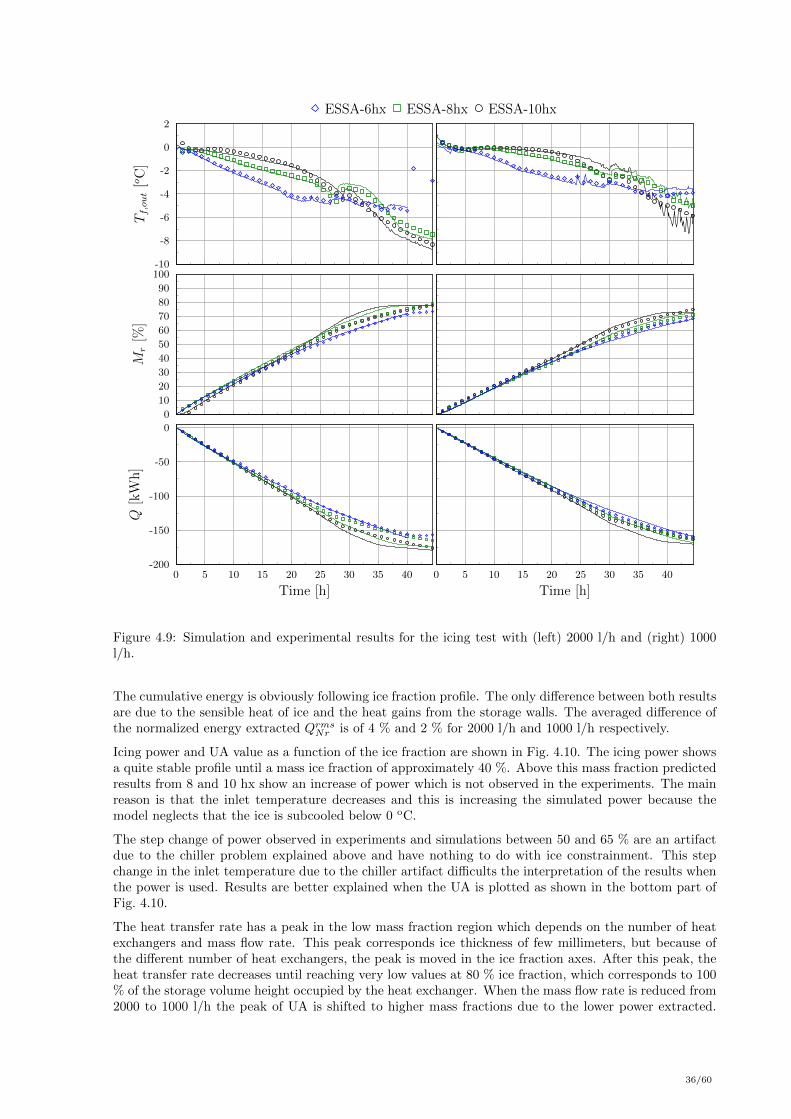
-10

-8

-6

-4

-2

0

2

Tf,out[oC]

0

10

20

30

40

50

60

70

80

90

100

Mr[%

]

-200

-150

-100

-50

0

Q[kW

h]

0 5 10 15 20 25 30 35 40

Time [h]0 5 10 15 20 25 30 35 40

Time [h]

ESSA-6hx ESSA-8hx ESSA-10hx

Figure 4.9: Simulation and experimental results for the icing test with (left) 2000 l/h and (right) 1000l/h.

The cumulative energy is obviously following ice fraction profile. The only difference between both resultsare due to the sensible heat of ice and the heat gains from the storage walls. The averaged difference ofthe normalized energy extracted QrmsNr is of 4 % and 2 % for 2000 l/h and 1000 l/h respectively.

Icing power and UA value as a function of the ice fraction are shown in Fig. 4.10. The icing power showsa quite stable profile until a mass ice fraction of approximately 40 %. Above this mass fraction predictedresults from 8 and 10 hx show an increase of power which is not observed in the experiments. The mainreason is that the inlet temperature decreases and this is increasing the simulated power because themodel neglects that the ice is subcooled below 0 oC.

The step change of power observed in experiments and simulations between 50 and 65 % are an artifactdue to the chiller problem explained above and have nothing to do with ice constrainment. This stepchange in the inlet temperature due to the chiller artifact difficults the interpretation of the results whenthe power is used. Results are better explained when the UA is plotted as shown in the bottom part ofFig. 4.10.

The heat transfer rate has a peak in the low mass fraction region which depends on the number of heatexchangers and mass flow rate. This peak corresponds ice thickness of few millimeters, but because ofthe different number of heat exchangers, the peak is moved in the ice fraction axes. After this peak, theheat transfer rate decreases until reaching very low values at 80 % ice fraction, which corresponds to 100% of the storage volume height occupied by the heat exchanger. When the mass flow rate is reduced from2000 to 1000 l/h the peak of UA is shifted to higher mass fractions due to the lower power extracted.

36/60

-7

-6

-5

-4

-3

-2

-1

0

Q[kW

]

0

1

2

3

4

5

6

7

8

UA

[kW

/K]

0 10 20 30 40 50 60 70 80

Mr [%]0 10 20 30 40 50 60 70 80

Mr [%]


Figure 4.10: Simulation and experimental results for the icing test as function of the mass ice fractionwith (left) 2000 l/h and (right) 1000 l/h.

The peak has the highest uncertainty because the outlet is closer to 0 oC reducing the logarithmic meantemperature difference. The UA is way off compared to experiments because an error in the outlettemperature leads to an error in the power predicted and also in the LMTD and, thereby, the UA addsall these errors. For example, a 6 % higher outlet temperature can lead to a 12 % lower power and 17 %higher LMTD. A division by this lower power divided by the higher LMTD leads to a 25 % lower UA.


Experimental and numerical results for the icing test are provided in Fig 4.11 and Fig 4.12 for (left) 2000l/h and (right) 1000 l/h for all CM tested. Quantified differences between simulations and experimentsare provided in Table 4.6.

The outlet temperature of the heat exchanger is shown in the upper part of Fig. 4.11 as a function oftime. Numerical predictions are in good agreement with experimental data with average differences ofT rmsf,out between all CM heat exchangers of 0.3 K and 0.6 K for 2000 l/h and 1000 l/h respectively. Theseabsolute RMS differences correspond to 3 % and 7 % respect to the total temperature difference of thetest (8 K for the icing case).

The ice fraction is shown in the middle section of Fig. 4.11. Very high ice fractions were achieved forall capillary mats and mass flow rates. No damaging of the casing was observed with any of the heatexchangers used. Regarding the simulations, with the exception of S-type-8hx case, the ice fraction isover-predicted by the simulated cases until the maximum predicted ice fractions is reached. The mainexplanation is that the model is neglecting the heat capacity of ice and therefore the energy extractedis used completely to ice. The maximum ice fraction observed in the experiments was not achieved inthe simulations for 16 number of heat exchangers, since some water volume was necessary to solve thesystem of equations.

The predicted cumulative energy extracted is following the same pattern as the mas fraction. Averagednormalised energy differences of all simulations QrmsNr in the order of 6 % and 7 % for 2000 l/h and 1000l/h respectively are found. The model developed for ice constrainment shows to work properly evenin the case of highly asymmetry between tubes, i.e. Stype-8hx. Differences between simulations and

37/60

experiments are more or less in the same order of magnitude for all cases. Thus, the model predictssimilarly both symmetric and highly non-symmetric heat exchangers configurations. Variations on thevolume flow are also predicted with similar accuracy.

Predictions of instantaneous power show higher differences compared to energy along the testing time.Differences in the order of 16 - 23 % of QNr,rms are observed in all cases. Heat power predictions areshown in Fig. 4.12 as a function of the ice fraction. Differences in Fig. 4.12 might not be correspondingexactly to what has been quantified in Table 4.6, because quantified differences differences presented inthe table are obtained with differences along the time. Fig. 4.12 shown results along the ice fractionand therefore results are coupled with prediction of the ice fraction too. The step changes in powerpredictions, e.g. at 50 % Mr for Stype-8hx are due to the artifact of the chiller and have nothing to dowith ice constrainment. UA values are very well predicted. The heat transfer rate UA for the icing test iscalculated in both experiments and simulations considering the storage water is at 0 oC. The temperaturesensors for water in the ice storage were covered with ice and temperatures were measuring values downto -7 oC and were obviously not representing the temperature of the liquid remaining water. The goodresults of the UA show that the model is able to predict appropriately the heat transfer with constrainedice under different heat exchangers set ups. Predictions of heat power show much larger differences,partially due to the simplification of considering that ice is always at 0 oC. As said before temperaturesensors in the storage were measuring values of -7 oC. Subcooling 2000 kg of ice to -7 oC needs about 8kWh, around 4 % of the total energy needed in the icing process. Therefore, it is of relevance and shouldbe included in future works.

Table 4.6: RMS differences between experiments and simulations for solidification test using capillarymats.

T rmsf,out Qrms QrmsNr Qrms QrmsNr

[K] [kW ] [%] [kWh] [%]

T5 : Icing with 2000 l/hCM-Gtype-16hx 0.39 0.87 20.17 7.23 6.29CM-Stype-16hx 0.37 0.79 21.54 9.60 6.91CM-Gtype-8hx 0.33 0.73 16.83 7.00 5.90CM-Stype-8hx 0.28 0.59 16.13 7.83 6.23θmax 0.4 0.9 21.5 9.6 6.9θavg 0.3 0.7 18.7 7.9 6.3

Icing with 1000 l/hCM-Gtype-16hx 0.77 0.87 22.97 8.00 6.77CM-Stype-16hx 0.66 0.73 16.97 5.96 4.91CM-Gtype-8hx 0.75 0.84 23.54 7.28 6.08CM-Stype-8hx 0.40 0.42 16.98 6.74 4.67θmax 0.8 0.9 23.5 8.0 6.8θavg 0.6 0.7 20.1 7.0 5.6

4.5. Melting cycle

The experiments for the melting cycle have been presented in section 2.6.4. The cycle consist on meltingthe ice of the storage with a set fluid temperature of 10 oC. However, as already discussed before, the fluidinlet temperature in the heat exchangers is changing over time because the chiller (heating device in thiscase) is connected directly to the heat exchangers and has not enough power to raise the temperature from0oC to 10 oC with the given volume flow. Each experiment started at a slightly different ice fraction due tothe whole testing sequence previous to the melting test sequence. All tests from sensible heating, coolingand icing were in series for each mass flow. However, between the icing and the melting experiments, acycling sequence was tested and thus, the initial Mr depends on the cycling test. Results from the cyclingtest are provided in section 4.6. The melting test sequence was finished when the storage temperaturewas at 10 oC approximately. After this sequence the whole process with 1000 l/h was started. This iswhy the sensible heating sequence for 1000 l/h starts at 10 oC and not at 20 oC.

The measurements of the ice fraction were not accurate for the melting process in all cases. Therefore, inorder to plot the ice fraction from the experiments, it has been calculated based on the energy extractedconsidering the sensible heat of water when being heated to 0 oC, but neglecting the heat losses thoughthe storage walls and the sensible heat stored in the ice.

38/60

-10

-8

-6

-4

-2

0

2

Tf,out[oC]

0

10

20

30

40

50

60

70

80

90

100

Mr[%

]

-250

-200

-150

-100

-50

0

Q[kW

h]

0 5 10 15 20 25 30 35 40

Time [h]0 5 10 15 20 25 30 35 40

Time [h]


Figure 4.11: Simulation and experimental results of CM for the icing test with (left) 2000 l/h and (right)1000 l/h.

-7

-6

-5

-4

-3

-2

-1

0

Q[kW

]

0

1

2

3

4

5

6

7

8

UA

[kW/K

]

0 10 20 30 40 50 60 70 80 90

Mr [%]0 10 20 30 40 50 60 70 80 90

Mr [%]


Figure 4.12: Simulation and experimental results for the icing test as function of the mass ice fractionwith (left) 2000 l/h and (right) 1000 l/h.

4.5.1 Flat plates

The predicted outlet temperatures of the heat exchanger and the averaged temperature of the storageare shown in Fig 4.13. RMS differences are presented in Table 4.7

39/60

The outlet temperature of the heat exchanger is shown in the upper graphs of Fig. 4.13. Predictions followrelatively well the experimental data. However, an overprediction of Tf,out is usually observed when thestorage is being heated up, i.e. when the sensible heating phase starts to be dominant. This means thatthe power is underpredicted when most of the ice has been already melt. The storage temperature isshown in the middle graphs of Fig. 4.13. At beginning of the test the sensors are covered with solidice and temperatures of -7 oC are measured. However, the value Tstore refers to the remaining watertemperature and therefore experimental results have been limited to ≥ 0 oC. Averaged RMS differencesof the outlet heat exchanger temperature T rmsf,out of 0.63 K and 0.84 K are observed for 2000 l/h and 1000l/h volume flows. These difference represent 6 % and 8 % respect to the temperature difference alongthe test (10 oC for melting test).

-2

0

2

4

6

8

10

12

Tf,out[oC]

-2

0

2

4

6

8

10

12

Tst,av[oC]

5 10 15 20 25 30 35

Time [h]5 10 15 20 25 30 35

Time [h]


Figure 4.13: Simulation and experimental results for the melting test with (left) 2000 l/h and (right)1000 l/h.

Table 4.7: RMS differences between experiments and simulations for melting test using flat plates.


[K] [kW ] [%] [kWh] [%]

T9 : Melting with 2000 l/hFP-SS-10hx 0.64 1.36 19.58 7.34 7.69FP-SS-8hx 0.70 1.49 22.10 6.38 6.49FP-SS-6hx 0.54 1.10 16.38 14.91 13.97θmax 0.70 1.49 22.1 14.9 14.0θavg 0.63 1.3 19.4 9.5 9.4

T9 : Melting with 1000 l/hFP-SS-10hx 0.73 0.75 13.37 5.77 5.56FP-SS-8hx 0.61 0.61 10.98 5.68 5.77FP-SS-6hx 1.06 1.13 20.98 4.28 4.20θmax 1.06 1.13 21.0 5.8 5.8θavg 0.80 0.8 15.1 5.2 5.2

The predicted cumulative energy provided to the storage, shown in Fig. 4.14, is relatively well predictedexcept for the case with 6 hx and 2000 l/h. For this case the Nusselt number for the natural convectionis underestimated. A reason could be the large distance between plates, allowing in one hand to easilydetach ice plates from the heat exchangers and in the other hand enhancing natural convection. Thedetachment of plates is not considered in the present model and this increases the heat transfer area

40/60

of ice plates since two surfaces are used to melt instead of the one close to the heat exchanger whennot detached. Averaged differences between heat exchanger units in normalized RMS cumulative energyQrms are in the order of 10 % and 63 %, with the largest difference of 14 % for 6 hx units and 2000 l/h.

0

10

20

30

40

50

60

70

80

90

100

Mr[%

]

0

20

40

60

80

100

120

140

160

180

200

Q[kW

h]

5 10 15 20 25 30 35

Time [h]5 10 15 20 25 30 35

Time [h]



The mass fraction of ice has been also plotted in Fig. 4.14 in order to know what was the initial icecontent for each case. For the experimental case, the M∗

r has been used, i.e. the ice fraction is calculatedusing the energy extracted since measures where not very accurate (see section 2.6.4 for details).

The melting power and the heat transfer rate UA are shown in Fig. 4.15 as a function of the ice fractionMr for simulations and ice corrected fraction M∗

r for the experiments. Notice that the test starts withthe highest ice fraction and, thereby, results at the beginning of the test are plotted in the right handside of the x-axis. The melting sequence can be split in three phases, the first one where heat conductionis dominant (Mr ≥ 60 % approx). When the melted plates are large enough, convection starts to bethe dominant effect. In the third phase (Mr ≤ 10 − 20 % approx), plates detach from heat exchangers.After the detachment, these plates are pushed towards the surface due to the density gradient betweenwater and ice and are melted faster due to the higher temperature on the upper part of the storage andalso due to the larger melting surface area, i.e. two faces per plate instead of the one close to the heatexchanger when attached to it are used for melting. The detachment of flat plates is not considered inthe present model.

In general the model underpredicts melting UA rates when conduction is dominant and also when iceplates are floating to the surface (low Mr values). The highest different is found with 6 hx and 2000l/h where the model clearly underestimates the melting power. Interestingly, predictions are in goodagreement when 6 hx and 1000 l/h are used. For 1000 l/h both experiments and simulations showa lower melting power compared to 8 hx and 10 hx units. For 2000 l/h simulations show the samebehaviors, i.e. predictions of lower melting power, but this is not observed in the experiments where thepower is very similar to that when 8 hx or 10 hx units are used.

The UA values are relatively well predicted during most of the convective dominant melting (20 ≥Mr ≤69). High differences are observed in the low ice fraction region (Mr ≤ 20), specially for 1000 l/h. Bothexperiments and simulations show a UA valley for 2000 l/h in the region 5 ≥ Mr ≤ 15. However,simulations tend to shift this valley towards higher ice fractions and the valley is more pronounced in thesimulations. For 1000 l/h this vally is not observed in the experiments and only slightly in the simulations.

41/60

In fact, experiments show a peak for 8 and 10 hx units, instead of a valley, at low ice fractions when1000 l/h are used. Probably plates are detached for these cases increasing the melting rates as explainedabove. Clearly, the phenomena of detachment uder this conditions is somewhat chaotic and difficult topredict. In the model presented in Carbonell et al. (2015), the detachment of ice plates was modelledfor a thermal de-icing concept. However, for when de-icing is used ice plates are always thin and theice from the tow faces of the heat exchanger are never in contact. Therefore, detachment of ice platescan be controlled and thus modelled. In the present case, plates can detach or not depending on manyphenomena that can not be modelled.

0

1

2

3

4

5

6

7

8

9

10

Q[kW

]

0

1

2

3

4

5

6

7

8

UA

[kW/K

]

0 10 20 30 40 50 60 70 80

M∗r [%]

0 10 20 30 40 50 60 70 80

M∗r [%]


Figure 4.15: Simulation and experimental results for the melting test as function of the corrected massice fraction with (left) 2000 l/h and (right) 1000 l/h. M∗

r is used for experiments and Mr for simulations.


The predicted outlet temperatures of the heat exchanger and the averaged temperature of the storageare shown in Fig 4.16. Quantified RMS differences for CM simulations are presented in Table 4.8.

The outlet temperature of the heat exchanger, shown in Fig. 4.16, is well predicted until sensible heatbecomes dominant. The storage temperature shown in the bottom part of Fig. 4.16 increases faster inthe simulations. This means that the power is overpredicted when most of the ice has been already melt.Averaged T rmsf,out RMS differences between all CM is of 0.6 K and 1.2 K are observed for 2000 l/h and1000 l/h volume flows.

The cumulative energy along with the ice fraction is shown in Fig. 4.17. All simulations end the meltingtest with lower energy values. There are two main reasons are this. The first one is that the whole blockof ice before being melted was at temperatures below 0 oC. All these energy is neglected in the model.Moreover, in some cases it is not possible to start the model with the same initial mass of ice than inthe experiments because the model needs some liquid water to solve the system of equations (see Eq.13). Besides these differences found at the end of the test, there is one case where differences are clearlylarger compared to the others, i.e. Stype-16hx. For this case the model is over-predicting the cumulativeenergy substantially with normalized RMS QrmsNr of 12 %. However, the averaged values for all cases arearound 6 % and 5 % for 2000 l/h and 1000 l/h respectively.

The melting power and heat transfer rates are shown in Fig. 4.18 respect to the ice fraction. Meltingrates for 2000 l/h are well predicted for G-type, but for S-type large differences are found. In general

42/60

Table 4.8: RMS differences between experiments and simulations for melting test using capillary mats.


[K] [kW ] [%] [kWh] [%]

T9 : Melting with 2000 l/hCM-Gtype-16hx 0.47 0.98 14.04 1.94 2.05CM-Stype-16hx 0.90 1.95 42.69 11.16 11.99CM-Gtype-8hx 0.27 0.54 11.68 5.21 6.08CM-Stype-8hx 0.70 1.53 27.84 5.06 5.01θmax 0.90 1.95 42.7 11.2 12.0θavg 0.58 1.2 24.1 5.8 6.3

T9 : Melting with 1000 l/hCM-Gtype-16hx 0.77 0.83 12.62 2.05 2.12CM-Stype-16hx 0.98 1.04 23.21 3.93 4.27CM-Gtype-8hx 0.70 0.68 15.08 2.33 2.71CM-Stype-8hx 1.85 0.80 16.69 2.33 2.67θmax 1.85 1.04 23.2 3.9 4.3θavg 1.07 0.8 16.9 2.7 2.9

-2

0

2

4

6

8

10

12

Tf,out[oC]

-2

0

2

4

6

8

10

12

Tst,av[oC]

5 10 15 20 25 30 35 40 45

Time [h]5 10 15 20 25 30 35 40 45

Time [h]



results for melting for S-type are significantly worst compared to the other cases. The reason, why it islike that, it is not clear yet. The melting power predicted for S-type-16hx is overpredicted during all thetest. For S-type-8hx the model overpredicts significantly the melting power for Mr ≤ 40 approximately.The melting power of Stype-8hx shows a different behaviour compared to all other cases with a cleardecrease of power for low ice fractions. However, the UA value shows a relatively constant value, whichmeans that the change of storage temperature makes the difference in the power predictions. For 1000l/h, melting power is much better predicted. Even though average normalized RMS power QrmsNr is inthe order of 16 % for 1000 l/h, most of the differences are at the end of the test when for simulations thepower tends to zero but experimental data still shows some power values due to the larger energy thatcan be extracted in experiments for the higher initial ice fraction and subcooling of ice.

43/60

0

10

20

30

40

50

60

70

80

90

100M

r[%

]

0

20

40

60

80

100

120

140

160

180

200

Q[kW

h]

5 10 15 20 25 30 35 40 45

Time [h]5 10 15 20 25 30 35 40 45

Time [h]



0

1

2

3

4

5

6

7

8

9

10

Q[kW

]

0

1

2

3

4

5

6

7

8

UA

[kW/K

]

0 10 20 30 40 50 60 70 80 90

M∗r [%]

0 10 20 30 40 50 60 70 80 90

M∗r [%]


Figure 4.18: Simulation and experimental results for the melting test as function of the mass ice fractionwith (left) 2000 l/h and (right) 1000 l/h. M∗

r is used for experiments and Mr for simulations.

44/60

4.6. Cycles of icing and melting

Simulated and experimental results of the test considering cycles of heating and cooling on icing andmelting conditions are shown in Fig. 4.19 for 1000 l/h and in Fig. 4.20 for 2000 l/h. The three testednumber of heat exchangers are shown in those figures, 6 hx in the left, 8 hx in the mid and 10 hx in theright side. In the upper part of the figures the simulated ice thickness is provided (left axes) and the inletand outlet temperature of the heat exchangers (right axis).

0.0

0.2

0.4

0.6

0.8

1.0

1.2

1.4

sice[cm]

sout-7 cm

-8

-6

-4

-2

0

2

4

6

8

10

Q[kW

]

-5

0

5

10

15

20

Qcycle[kW

h]

0 1 2 3 4 5 6 7 8 9 10

Time [h]

sout-5 cm

0 1 2 3 4 5 6 7 8 9 10

Time [h]

-8

-6

-4

-2

0

2

4

6

8

10

T[oC]

sout-4 cm

0 1 2 3 4 5 6 7 8 9 10

Time [h]

Symbols : experimental Solid lines : simulations

Tin Tout sin smelt

Figure 4.19: Simulation and experimental results of the icing and meting cycle T8 with 1000 l/h for (up)FP-6hx (mid) FP-8hx and (bot) FP-10hx.

The simulated ice thickness is shown for the outlet thickness sout, for the internal thickness sin and forthe melted thickness smelt. Explanations of these thickness are provided in section 3 . The fix constantvalue per set of heat exchangers has been subtracted from the outlet ice thickness in order to plot allresults with a smaller range, e.g. for 6 hx the outlet ice thickness is reduced by 7 cm is order to beplotted in the range of 0 to 1.4 cm. The power for melting and icing is shown in the mid part of thefigures. The cumulative energy provided by the heat exchangers Qcycle for melting and icing for eachheating and cooling cycle is shown in the bottom part of each figure. All the cycling test starts with a

45/60

melting phase that last until the experimental outlet temperature of the heat exchanger is above 0 oC.This phase is needed in order to ensure that the cycling test allows to melt and ice. Otherwise the heatingand cooing cycles could only change the temperature from the ice from -8 oC to 0 oC without actuallymelting any ice. The model is not prepared to work under the subcooled zone and the solid ice is alwaysassumed to be at 0 oC. This is the reason why in all cases simulated results in the first meting phase arealways over-predicting the temperature and thus under-predicting the power and the melted energy. Inthe experiments the ice is at temperatures down to -8 oC increasing the extracted power respect to thesimulations where the ice is assumed to be at 0 oC. In this initial phase the outlet ice thickness decreasesrapidly as the melted ice thickness increases. After this initial phase the icing and melting cycles start.In each cycle of icing and melting the internal ice thickness increases reducing the melted ice thicknessand increasing the total ice thickness correspondingly. When a second cycle starts, if the internal icethickness has not reached the melted ice the internal ice thickness is assumed to stick to the external icethickness. As soon as the internal ice thickness reaches the melted thickness, the melted and internal icethickness are set to zero and the whole ice thickness is in one block. This can be observed in Fig. 4.20after the first cycle for 6 hx (left graphs), between 1 and 2 hours.

0.0

0.2

0.4

0.6

0.8

1.0

1.2

1.4

sice[cm]

sout-7.5 cm

-8

-6

-4

-2

0

2

4

6

8

10

Q[kW

]

-5

0

5

10

15

20

Qcycle[kW

h]

0 1 2 3 4 5 6 7 8 9 10

Time [h]

sout-5 cm

0 1 2 3 4 5 6 7 8 9 10

Time [h]

-8

-6

-4

-2

0

2

4

6

8

10

T[oC]

sout-4 cm

0 1 2 3 4 5 6 7 8 9 10

Time [h]

Symbols : experimental Solid lines : simulations

Tin Tout sin smelt

Figure 4.20: Simulation and experimental results of the icing and meting cycle T8 with 2000 l/h for (up)FP-6hx (mid) FP-8hx and (bot) FP-10hx.

46/60

Looking at the temperature of the heat exchanger for 1000 l/h it can be seen that in the experimentsthe outlet temperature is very stable at 0 oC even when the inlet is at 7 oC. This is probably due to thesensible “cold” accumulated in the ice. The outlet predicted temperatures in the icing mode are usuallywell predicted and close to 0 oC except when the internal ice thickness reaches the melted thickness. Inthis circumstances, the ice resistance increases because all ice thickness in in one block and thereforethe outlet temperature decreases when icing. This is not observed in the experiments because in realitymultiple ice layers are possible and the icing always start to form without any ice on the surface (whichis not the case in the model after sin reaches smelt). Both the power and the energy for melting and icingagrees very well with the experimental data.

4.7. Conclusions

In this chapter, the mathematical formulation for an ice storage has been validated with experimentaldata from chapter 2. Validation of the model has been conducted using a large number of simulatedcases, including difference testing sequences, heat exchanger types, number of heat exchangers and massflow rates. The parameters of the model were constant for all cases, without any specific tuning per caseof heat exchanger type. The main conclusions of this chapter are:

• The sensible heating test is very well predicted by both FP and CM heat exchanger models. Thenormalized averaged energy differences QrmsNr are between 2 % and 6 % depending on mass flow andheat exchanger type. The normalized averaged power QrmsNr shows differences between 4 % and 7% for FP. For CM and 2000 l/h, differences of 5 % were observed. For CM and 1000 l/h, higherdifferences up to 13 % were observed. However, this was thought to be related to the non-steadyconditions at the beginning of the test and not to the mass flow rate influence.

• The sensible cooling test is not as well predicted as the heating case due to the differences betweensimulations and experiments around 4 oC, where the maximum density of water is found. Differencesin this region lead to higher differences in power predictions, with averaged QrmsNr between 7 % to 11% depending on mass flow and heat exchanger type. Nevertheless, differences in energy predictionswere found to be good with QrmsNr between 2 % to 5 %.

• The validation of the icing test was found to be very challenging for the CM and specific functionsto mode the ice constrainment were necessary to handle different distances between tubes in twospatial direction. In FP these functions are not necessary due to the unidirectional growing of theice in the heat exchanger plates. Energy differences and thus ice fraction evolution were found tobe satisfactory with averaged differences of QrmsNr between 2 % to 6 %. However, power predictionshad larger errors with difference of QrmsNr around 22 to 25 % for FP and around 20 % for CM.

• The validation of the melting process lead to similar results to the icing test. Averaged QrmsNr werebetween 5 % to 9 % for FP and between 3 % to 6 % for CM. Averaged differences in power werebetween 15 % to 19 % for FP and between 17 % to 25 % for CM depending on mass flow rate.

5. Solar-ice system simulations

The aim of the present chapter is to analyze flat plates (FP) and capillary mats (CM) heat exchangersfor solar-ice systems. The optimum heat exchanger area needed in the ice storage is based on energetictransient system simulations and on cost indicators. In section 5.1 the methodology followed to solve thesystem of equations is described, in section 5.2 the hydraulics of the system are presented. In section 5.5,the results of the simulation from an energetic point of view are presented and the cost of the systemsare discussed in section 5.6.

5.1. Methodology

Dynamic system simulations are used in order to assess the heat exchanger area and heat exchanger typeon a system level. The simulations have been conducted with the simulation environment TRNSYS-17 (Klein et al., 2010). The basic components to model a solar-ice system are: collectors, heat pump,ice storage, sensible thermal storage, building, climate and control. The ice storage model has been

47/60

explained in chapter 3. The formulation of the remaining component models were provided in Carbonellet al. (2016c), where a complete solar-ice system based on a de-icing concept was validated with monitoreddata on one pilot plant.

The time step of yearly simulations is set to 120 seconds. As a verification process several systematicchecks are done for all simulations. Heat balances are checked in all individual components, hydraulicloops and also from the system perspective. The convergence criteria from TRNSYS is set to 5e-4, whichallows to achieve heat imbalances always below 1.% in respect to the total demand. Iteration problemsare also checked for all simulations and are always below 10 time steps per year simulated. In most casesiteration problems are in the order of 1 - 5 per year.

5.2. Hydraulic scheme of the simulated system

The hydraulic scheme of the complete solar-ice heating system is shown in Fig. 5.1. The main componentsof the heating system are the collector field, the combi-storage, the heat pump and the ice storage.

Figure 5.1: Simplified hydraulic scheme of the analysed heating system.

The main energy source of the system is the solar irradiation. Some additional energy is extracted fromthe air, especially when uncovered collectors are used 4. Part of the total solar irradiation is transformedby the collectors to useful heat for the system. This energy is transferred, either to the heat pump, to theice storage or to the combi-storage. When the heat pump is running, two operation modes are possible,depending on whether the collectors are able to provide energy or not: i) the heat pump uses the solarenergy directly in a series operation mode or ii) the heat pump uses the ice storage as its source. Withthe hydraulic set-up proposed here, when the heat pump is running with solar energy as a source, themass flow from the solar collector field is divided: one part goes to the heat pump and the other partgoes to the ice storage. The split of the mass flow is basically controlled by each pump, i.e. solar andheat pump evaporator. If these mass flows are not equal, its difference will flow to the ice storage. Onthese conditions, if more energy is available from the collector field than is needed by the heat pump,the ice storage is also loaded while the heat pump is running. On the contrary, if the collector output islower than the heat pump needs, both, the ice storage and the collector field are used to provide heat tothe evaporator of the heat pump. If none of these heat sources are available, which means that the icestorage is full of ice and the solar radiation and the ambient temperature are very low, the temperatureof the heat pump evaporator drops below the minimum allowed value and the heat pump stops. In thiscase, a direct electric back-up is used. A method to reduce the need of back-up in winter times is to sendthe whole mas flow from the collector to the heat pump. This can be done with this hydraulic schemeby setting the mass flow from the collector equal to the one demanded by the heat pump. This tendsto reduce the working temperature of the circuit and as a consequence decrease the heat pump COP.However, it reduces the times where the ice storage is used and thus the times where the direct electricback-up is used. Usually, reduction of the time use of the back-up is compensated by the loss of heatpump performance.

4All results shown in this project are obtained with selective uncovered collectors.

48/60

5.3. System control

The system part on the secondary side of the heat pump, i.e. the heating distribution and the DHW-preparation, and the heat pump itself are mostly controlled in a standard way. The brine cycle on theprimary side, on the other hand, needs some special operation modes to decide how to use the solar heat.The backup needs to be controlled too, such that it runs when there is a heating demand in the buildingand the ice storage is fully iced (no source available for the heat pump). Further, season-based prioritiesregarding the use of the solar heat are implemented. The solar-ice system has a global control with threemain priorities in the following hierarchy:

1. Use of direct solar heat to provide the space heat to the building without switching on the heatpump.

2. Switching on the heat pump when not enough energy is available in the combi-storage in order toprovide the space heat. When heat pump is on, solar energy is prioritized as energy source.

3. Use solar heat to load the combi-storage and ice storage when the heat pump is off. Loading thecombi-store is usually referred as direct solar heat. Direct solar heat is usually prioritized in spring,summer and autumn, but in winter the loading of the ice storage is prioritized.

The control has to cope with the fact that the ice storage is a cold sink for a long time during the year.Unless a logic is implemented, that switches to loading of the combi-storage when appropriate, the icestorage would be loaded predominantly. The control mode that actively stops the loading of the coldstorage and tries to divert the solar heat on a higher temperature level to the combi-storage is calledwarm storage priority. If the warm storage priority is not active, the control mode cold storage priorityis on, which loads the ice storage. For small sized systems is usually a better option to use the a coldstorage priority in winter in order to avoid the time when the direct electric back-up is needed. As soonas there is no risk to fully ice the storage, then warm storage priority should be used.

5.4. Performance indicators

The main performance indicator for the systems is the System Performance Factor calculated as describedin Malenkovic et al. (2012):

SPFSHP+ =QDHW +QSH

Pel,T=

QDPel,T

(44)

Q is the yearly heat load energy and Pel,T the total yearly electric energy consumption. The subscriptsSHP , DHW , SH and D stand for solar and heat pump, domestic hot water, space heating, and totaldemand respectively.

The total electricity consumption is calculated as:

Pel,T = Pel,pu + Pel,hp + Pel,cu + Pel,aux + Pel,pen (45)

where the subscripts pu, hp, cu, aux and pen refer to circulation pumps, heat pump, control unit, auxil-iary and penalties respectively. The symbol ”+” in the SHP+ from Eq. 44 refers to the consideration ofthe heat distribution circulating pump in the electricity consumption. Therefore, the system performanceindicator used in this work includes all circulation pumps of the system and also all thermal losses/gainsfrom storages and piping. Penalties for not providing the heating demand at the desired comfort temper-ature are calculated according to Haller et al. (2012). Pel,aux is the energy used from the direct electricback-up system.

5.5. System energetic performance with varying heat exchanger type and area

Dynamic yearly system simulations have been carried out for different heat exchanger areas and for twotypes of heat exchangers, capillary mats (CM) and flat plates with stainless steel (FP-SS). Simulationshave been performed for ice storage volumes of 3 m3, 4 m3 and 5 m3 and collector areas of 15 m2, 20 m2

and 25 m2.

49/60

Vice = 3 m3 Vice = 4 m3 Vice = 5 m3

2.0

2.5

3.0

3.5

4.0

4.5

5.0

5.5

6.0

6.5

SPFSHP+

0 5 10 15 20 25 30 35 40

Ahx/Vice [m2/m3]

2.0

2.5

3.0

3.5

4.0

4.5

5.0

5.5

6.0

6.5

SPFSHP+

0 5 10 15 20 25 30 35 40 45 50 55 60

Distance Hx [cm]

0 5 10 15 20 25 30 35 40

Ahx/Vice [m2/m3]

0 5 10 15 20 25 30 35 40 45 50 55 60

Distance Hx [cm]

0 5 10 15 20 25 30 35 40

Ahx/Vice [m2/m3]

0 5 10 15 20 25 30 35 40 45 50 55 60

Distance Hx [cm]

CM, Acol = 15 m2

CM, Acol = 20 m2

CM, Acol = 25 m2

FP-SS, Acol = 15 m2

FP-SS, Acol = 20 m2

FP-SS, Acol = 25 m2

Figure 5.2: Yearly system performance as function of (top) heat exchanger area divided by ice storagevolume and (bottom) distance between heat exchangers for three ice storage volumes of (left) 2 m3, (mid)4 m3 and (right) 5 m3.

Results for the SPFSHP+ are shown in Fig. 5.2 as a function of the ratio between the heat exchanger areaand the ice storage volume and as a function of the distance between heat exchangers. The same distancesbetween heat exchangers are used both for CM and FP-SS. However, since FP-SS have almost twice thearea5 compared to CM, results for FP-SS are shifted towards higher Ahx/Vice. Both heat exchangertypes are able to provide very high SPFSHP+, up to 6 for the sizes used in these simulations. Systemperformances above 4 (as GSHP) are always achieved if the collector area is ≥ 20 m2. For collector areasin the order of 15 m2, an SPFSHP+ above 4 can be achieved with CM and Vice = 4 m3 and with FP-SSif Vice = 5 m3. Using 15 m2 and 5 m3 both heat exchangers are able to provide SPFSHP+ above 4.

Very high system performances, in the order of 5 to 6, can be achieved with different component sizes.These results confirm the flexibility of the system concept, i.e. the same SPFSHP+ can be obtainedusing different configurations of ice storage volume and collector area. This allows to achieve an specificSPFSHP+ even if there are restrictions such as small cellar capacity or available roof area. However, thereis a limit on the lowest size of the collector field since the solar-ice system is based purely on solar energyas heat source. The system flexibility of solar-ice systems was discussed in Carbonell et al. (2014). Ofparticularly interest are results with 4 m3, since this storage volume could fit in many cellars of singlefamily homes using two separated storages of 2 m3 allowing to achieve an SPFSHP+ ≥ 5 with collectorareas of 20 m2.

Regarding the heat exchanger type, it seems clear that the SPFSHP+ is usually higher for CM comparedto FP-SS except for large distance between heat exchangers, e.g. > 25 cm for Vice =3 m3. Systemperformances for CM when distances between heat exchangers are small are higher because of the betterheat transfer coefficient when icing at high ice fractions. The SPFSHP+ of CM is worse than that ofFP-SS for cases where the distance between heat exchangers is way higher than that between the tubesin one CM. One can imagine a CM like a FP with empty spaces between tubes. Let’s imagine the limitcase where all tubes in one CM are in contact to each other. Under those circumstance CM would beworst than FP because of the higher resistance of polypropylene compared to stainless steel. When icefills all the gaps between tubes, there is the added limitation that not all area is used due to the spacesbetween tubes.

5The two faces of the flat plate heat exchanger are considered as heat exchanger area.

50/60

Differences between FP-SS and CM are more prominent for low collector areas and low ice storagevolumes. Results for 25 m2 and 5 m3 tend to an asymptotic solution where differences between CMand FP-SS are negligible. In those situation the direct electric back-up is not used because the systemcomponents are sized largely enough such that not all the latent heat capacity of the storage is necessary.The direct electric back-up is shown in Fig. 5.3 as a function of the ratio between Ahx and Vice. Clearly,


0.0

0.5

1.0

1.5

2.0

2.5

Qaux[M

Wh]

0 5 10 15 20 25 30 35 40

Ahx/Vice [m2/m3]

0 5 10 15 20 25 30 35 40

Ahx/Vice [m2/m3]

0 5 10 15 20 25 30 35 40

Ahx/Vice [m2/m3]

CM, Acol = 15 m2

CM, Acol = 20 m2

CM, Acol = 25 m2

FP-SS, Acol = 15 m2

FP-SS, Acol = 20 m2

FP-SS, Acol = 25 m2

Figure 5.3: Direct electric back-up as a function of heat exchanger area divided by ice storage volume forthree ice storage volumes of (left) 2 m3, (mid) 4 m3 and (right) 5 m3.

the increase of collector area and storage volume decrease the use of the direct electric back-up. Thedirect electric back-up is used exclusively in winter, when the ice storage if full (maximum ice fraction of80 % has been assumed) and there is not enough solar energy to provide the heat for the evaporator of theheat pump. The use of the electric back-up is the dominant factor that influences the SPFSHP+. Oncethe electric back-up is avoided, the system performance is quite independent of the heat exchanger areaand less dependent on the collector area or ice storage volume. A SPFSHP+ value below 5.5 is usuallyindicates the need of direct electric back-up.

In order to establish the optimum heat exchanger area in terms of SPFSHP+ it is of importance toinvestigate the maximum ice fraction achieved, as shown in Fig. 5.4. If the heat exchanger area is toolow for the specific system design, some latent heat may not be used because the heat transfer coefficientwill be too low at the maximum ice thickness achieved. This would lead to a situation where the heatpump would not be able to extract enough power from the ice storage while there is still liquid waterpresent. For CM the maximum ice fraction of 80 % is reached approximately for ratios of Ahx/Vice of5-10 m2/m3. For FP the maximum ice fraction is reached at higher ratios of 10-15 m2/m3. For bothcases these ratios correspond to a distance of around 7-12 cm between heat exchangers.

For some configurations, it is not possible to use all latent heat of the storage. For example for Vice = 5m3 and Acol = 25 m2, non of the heat exchangers setup can achieve an ice fraction of 80 %. This indicatesthat the system is oversized and either the ice storage or the collector area could be decreased and thesystem performance would not be penalized much. For example in Fig. 5.2 the SPFSHP+ of Acol = 25m2 is almost the same if the storage volume is 4 m3 or 5 m3. Another way to make use of the latent heatand also to increase the SPFSHP+ would be to give more priority to the warm storage loading.

5.6. Cost analyses of solar-ice systems

In sections above the system performance in terms of energy have been provided. In this section, costsare taken into consideration in order to further evaluate different system designs. For all analyzed heatingsystems, investment costs and heat generation costs for prices of the Swiss energy market in 2016/2017are calculated. The comparison of costs is used to find the optimum heat exchanger area consideringboth energetic system performance and a good value for the money.

The investment costs of the solar-ice systems are based on real costs that were gathered from severalsources. Some data was obtained from the realization of two demonstration projects of solar-ice systemsin Rapperswil-Jona, Switzerland. The data from the solar part was obtained from the SFOE project

51/60


0

10

20

30

40

50

60

70

80

90

100

Mr[%

]

0 5 10 15 20 25 30 35 40

Ahx/Vice [m2/m3]

0

10

20

30

40

50

60

70

80

90

100

Mr[%

]

0 5 10 15 20 25 30 35 40 45 50 55 60

Distance Hx [cm]

0 5 10 15 20 25 30 35 40

Ahx/Vice [m2/m3]

0 5 10 15 20 25 30 35 40 45 50 55 60

Distance Hx [cm]

0 5 10 15 20 25 30 35 40

Ahx/Vice [m2/m3]

0 5 10 15 20 25 30 35 40 45 50 55 60

Distance Hx [cm]

CM, Acol = 15 m2

CM, Acol = 20 m2

CM, Acol = 25 m2

FP-SS, Acol = 15 m2

FP-SS, Acol = 20 m2

FP-SS, Acol = 25 m2

Figure 5.4: Maximum yearly mass ice fraction as a function of (top) heat exchanger area divided by icestorage volume and (bottom) distance between heat exchangers for three ice storage volumes of (left) 2m3, (mid) 4 m3 and (right) 5 m3.

ReSoTech (Philippen et al., 2016). This data was used to derive cost functions per component. The costfunctions are then used to calculate investment costs per specific system size simulated.

A ground source heat pump system is used as a reference to compare the system performance in termsof energetic efficiency and cost. Using a borehole length of 130 m for a single family house in the regionof Zurich an SPFSHP+ around 4 is expected. Investment costs for GSHP are based on two offers of Swisssellers for a GSHP system that supplies heat to a single family house (Causi, 2010). The cost functionswere derived from average costs of the two offers. All received cost functions were verified by a Swissseller of heating systems in terms that they represent actual average market prices.

For each system the present value of costs and the annuity are calculated following the methodology ofVDI (2012) and Bangerter (1985) with some simplifications. Main assumptions for the economic analysisare given in Table 5.1 and details for the calculation method were provided in Philippen et al. (2015).The electricity prices are taken from the price list of a regional Swiss utility and represent typical pricesfor small customers. The increase of electricity cost is based on the assessment of this utility.

Table 5.1: Assumptions for calculation of heat generation costs.

Rate of interest 2.0 % p.a.Analysis period 25 yearsYearly Maintenance 0.25 % of investment costsLifetime ice storage casing and bore holes 50 yearsElectricity costs (incl. VAT) Fixed costs: 171 Fr. per year

Variable costs: 0.13 Fr. per kWhIncrease of electricity costs 1. % p.a.

52/60

5.6.1 Heat generation cost

The system performance (top) and the heat generation cost (bottom) are shown in Fig. 5.5 as a functionof the ratio Ahx/Vice for CM and FP-SS for three collector areas and storage volumes analyzed in sectionsabove. The SPFSHP+ is repeated here in order to compare directly graphs of SPFSHP+ and cost. Thereference values for the GSHP system are included in all graphs. The objective is to achieve a solar-icesystem with same or higher performance than GSHP with same or lower cost. Therefore, the focus is onsolar-ice systems with an SPFSHP+ ≥ 4. The only configurations where this target is not met are thesystems with Ac = 15 m2 and Vice = 3 m3. For Vice = 5 m3 all systems performance are above 4 and forVice = 4 m3 only performance of the case with 15 m2 and FP-SS are below 4.


2.0

2.5

3.0

3.5

4.0

4.5

5.0

5.5

6.0

SPFSHP+

28

30

32

34

36

38

40

Heatgenerationcost

[Rp./kW

h]

0 2 4 6 8 10 12 14 16 18 20

Ahx/Vice [m2/m3]

0 2 4 6 8 10 12 14 16 18 20

Ahx/Vice [m2/m3]

0 2 4 6 8 10 12 14 16 18 20

Ahx/Vice [m2/m3]

CM, Acol = 15 m2

FP-SS, Acol = 15 m2CM, Acol = 20 m2

FP-SS, Acol = 20 m2CM, Acol = 25 m2

FP-SS, Acol = 25 m2Ref : GSHP

Figure 5.5: System performance (up) and heat generation cost (bottom) as function of heat exchangerarea divided by ice storage volume. Three ice storage volumes are used: (left) 3 m3, (mid) 4 m3 and(right) 6 m3.

The heat generation cost are shown in bottom part of Fig. 5.5. There are two configurations wherethe SPFSHP+ ≥ 4 and the heat cost are below that from the GSHP. Both configurations are using CMand 15 m2, for 4 and 5 m3 storage volumes. These two system set-ups are of particular interest due tothe low cost and high efficiency. All systems using FP which performance is above 4 have higher heatgeneration cost compared to that of the GSHP. It should be noted that cost calculations are based onmany assumptions that affect significantly the results. Therefore, heat generation cost should be seen asorders of magnitude. Unfortunately, the error band is not easy to assess.

Using the cost function alone is not a good approach to decide the heat exchanger area. For examplein FP the lowest area seems to provide the cheapest system even when the energetic performance isrelatively low. Besides the cost function, the SPFSHP+ and also the maximum ice fraction achieved asshown in Fig. 5.4 should be used. Considering all these values it seems that the optimum heat exchangerarea is in the order of 4-5 m2/m3 for CM and around 10-14 m2/m3 for FP-SS. Those ratios correspondapproximately to 12-17 cm for both heat exchangers.

The heat generation cost along with the system performance are shown in Fig. 5.6 as a function of the

53/60

collector area. The heat generation cost increases linearly with collector area. The minimum of thefunction can not be observed with the simulated collector area. From this plot and the sizes chosen,it seems that is a better option to reduce the collector area and increase the ice storage volume. Forexample CM with Vice = 5 m3 and 15 m2 has higher SPFSHP+ and lower cost compared to CM with 20m2 of collector area. The cost of the selective uncovered collectors are based on a single manufacturer.Considering the cost of other manufacturers could change this trend.

2.0

2.5

3.0

3.5

4.0

4.5

5.0

5.5

6.0

6.5

7.0

SPFSHP+

15 20 25

Acol [m2]

28

30

32

34

36

38

40

Heatgenerationcost

[Rp./kW

h]

15 20 25

Acol [m2]

2.0

2.5

3.0

3.5

4.0

4.5

5.0

5.5

6.0

6.5

7.0

SPFSHP+

15 20 25

Acol [m2]

28

30

32

34

36

38

40

Heatgenerationcost

[Rp./kW

h]

15 20 25

Acol [m2]

Distance between heat exchangers 12.5 cm

Distance between heat exchangers 16.6 cm

CM, Vice = 3 m3

FP-SS, Vice = 3 m3CM, Vice = 4 m3

FP-SS, Vice = 4 m3CM, Vice = 5 m3

FP-SS, Vice = 5 m3Ref : GSHP

Figure 5.6: System performance (left) and heat generation cost (right) as function of the collector areaand ice storage volume for a distance of 12.5 cm (up) and 16.6 cm (bottom) between heat exchangers.

5.6.2 Installation cost

Installation costs for an ice storage volume of 4 m3 with a distance of 16.6 cm between each heat exchangerand a collector area of 15 m2 are shown in Fig. 5.7. As a reference, the installation cost of GSHP arecalculated as 53’048 Fr. The installation cost using CM heat exchangers, with a total amount of 48’460Fr., is 8.6 % lower than that of the GSHP and the case with FP-SS with 52’980 Fr. is almost the same.

An example of the calculation cost for the CM is shown in Table 5.2. The installation cost using FP-SSonly differ on the heat exchangers used in the ice storage. The cost of the ice storage for FP-SS is givenin Table 5.3.

The conclusions of the cost-energetic study of chapter 5 are provided at the end of the following chapter6.

54/60

Collectors

26.6%

Heat Pump

16.0%

Sensible Storage 13.1%

Ice Storage

21.7%

Labour

22.6%

Total cost 52.98 [kFr]

(a)

Collectors

29.1%

Heat Pump

17.5%

Sensible Storage

14.3%

Ice Storage

14.3%

Labour

24.8%

Total cost 48.46 [kFr]

(b)

Figure 5.7: Shares of installation cost for an ice storage of 4 m3 with a distance of 15 cm between heatexchangers and a collector area of 15 m2 for (a) FP-SS (b) CM.

Table 5.2: System and Heat generation costs for an ice storage of 4 m3, a distance of 16.6 cm betweenheat exchangers and a collector area of 15 m2 using CM heat exchangers (all values incl. 8% VAT).

Component Component Costs Total Costs[Fr.] [Fr.]

Ice Storage Stainless steel storage with insulation 5288CM heat exchangers 816

Piping 248Mounting heat exchangers and pipes 600

Total Ice storage 6953 (14%)

Collectors Selective uncovered 7935Hydraulic roof to cellar (solar) 6163

Total Collectors 14098 (29%)

Heat pumpHeat pump unit 7904

Hydraulic heat pump to combi-storage 186Insulation pipes 400

Total Heat pump 8490 (18%)

Thermal storages Basic costs storage 6915Total combi-storage 6915 (14%)

Labor cost Installation 8000Third parties + Divers 4000

Total Labor costs 12000 (25%)

Total Investment Cost 48456

Table 5.3: Ice storage cost for a volume of 4 m3 and a distance of 16.6 cm between each FP-SS heatexchanger (all values incl. 8% VAT).

Component Component Costs Total Costs[Fr.] [Fr.]

Ice Storage Stainless steel storage with insulation 5288FP-SS heat exchangers 4021

Piping 248Mounting heat exchangers and pipes 1920

Total Ice storage 11478 (22%)

55/60

6. Conclusions

In this research study a experimental and numerical analyses of different heat exchangers, i.e. capillarymats, flat plates and coils were carried out. An ice storage model able to cope with all analyzed heatexchangers has been developed and validated with the experimental data. The energetic simulationsof the complete solar-ice system has been used to find the optimum heat exchanger area for the mostpromising heat exchangers in terms of energetic efficiency and heat generation cost.

In chapter 2, results of several heat exchangers have been analyzed, including capillary mats with differentdesigns made of polypropylene, flat plates made of stainless steel and polypropylene and a custom-madepolypropylene coil. The area analyzed has been modified for each heat exchanger and all tests havebeen performed using two different mass flow rates. In total, ten possibilities have been experimentallyevaluated for several test sequences including sensible heating and cooling, icing, melting and cycling.The main conclusions of this experimental study can be summarized as:

• Very high ice fraction can be reached with all heat exchangers and mass flows.

• The casing did not show any damage under high ice fraction conditions. This means that designingan ice storages able to reach 95% ice fraction or higher should be safe.

• All heat exchangers showed to be reliable and robust under the test conditions. Long term testswere not carried out.

• Flat plates made of stainless steel are better suited compared to capillary mats or coils for sensibleheating and cooling and for melting processes.

• Capillary mats or coils are better suited compared to flat plates for the icing process due to thestrong decrease of performance that flat plates suffer when ice grows.

• Flat plates made of polypropylene have shown the worst thermal performance of all tested heatexchangers.

• Coil heat exchangers made of polypropylene for small ice storages were difficult to design and build.Therefore, it does not seem to be the a promising solution for low ice storage volume (< 5 m3).

From all the heat exchangers analyzed experimentally, capillary mats made of polypropylene and flatplates made of stainless steel are the most promising solutions.

In chapter 3 the mathematical model for an ice storage has been presented. The validation of the icestorage has been presented in chapter 4 using the experimental data from chapter 2. The main conclusionsof the validation procedure are:

• The sensible heating test is very well predicted by both FP and CM heat exchanger models. Thenormalized averaged energy differences QrmsNr are between 2 % and 6 % depending on mass flow andheat exchanger type. The normalized averaged power QrmsNr shows differences between 4 % and 7% for FP. For CM and 1000 l/h, higher differences up to 16 % were observed. However, this wasthought to be related to the non-steady conditions at the beginning of the test and not to the massflow rate influence.

• The sensible cooling test is not as well predicted as the heating case due to the differences betweensimulations and experiments around 4 oC, where the maximum density of water is found. Differencesin this region lead to higher differences in power predictions, with averaged QrmsNr between 7 % to 10% depending on mass flow and heat exchanger type. Nevertheless, differences in energy predictionswere found to be good with QrmsNr between 2 % to 5 %.

• The validation of the icing test was found to be very challenging for the CM and specific functionsto mode the ice constrainment were necessary to handle different distances between tubes in twospatial direction. The use of these functions were found to be satisfactory, since results using themlead to slightly better results for CM compared to FP. In FP these functions are not necessary dueto the unidirectional growing of the ice in the heat exchanger plates. Energy differences and thusice fraction evolution were found to be satisfactory with averaged differences of QrmsNr between 5 %to 6 %. However, power predictions had larger errors with difference of QrmsNr around 18 to 20 %for CM and between 25 to 30 % for FP depending on mass flow rate.

56/60

• The validation of the melting process lead to similar results to the icing test. Averaged QrmsNr werebetween 4 % to 6 % for FP and between 9 % to 10 % for CM. Averaged differences in power werearound 20 to 23 % for both FP and CM.

In general results are satisfactory considering the large number of simulated cases, including differencetesting sequences, the use of different heat exchanger types, number of heat exchangers and the use ofdifferent mass flow rates. Moreover, the parameters of the model were constant for all cases, withoutany specific tuning per case of heat exchanger type. Therefore, results should be compared with cautionto other publications were only one case was simulated. Tuning each case could reduce the differencessignificantly.

In chapter 5 the complete solar-ice system has been simulated with the validated ice storage model fromchapter 3. From the system simulations the following conclusions can be drawn:

• A solar-ice system with ice storages volumes between 0.3 to 0.5 m3 per MWH of yearly heatingdemand, and collector areas between 1.6 to 2.6 m2/MWh can reach an SPFSHP+ in the range of3.5 to 6 in Zurich for a single family home with 9.5 MWh total (SH + DWH) heating demand.

• Besides the sizes of the ice storage and collector field areas, the most relevant factor affecting theSPFSHP+ is the electric back-up necessary to run the system in winter periods. Control strategiesshould be focus on reducing it as a first target. When the electric back up is minimized, controlstrategies should focus on the maximization of direct solar heat.

• Solar-ice systems can reach very high SPFSHP+ regardless of the heat exchanger type, but whenthe heat generation cost are included, only capillary mats are able to provide higher SPFSHP+

compared to GSHP at a lower cost. However, the heat exchanger area needs to be well design toreach these targets. An ice storage volume of 0.5 m3/MWh with capillary mats and 1.6 m2/MWhof collector area can reach heat generation costs of 29 Rp./kWh (0.5 Rp./kWh below the GSHP)with an SPFSHP+ of 4.8, which represents an increase of SPFSHP+ of 20 % respect to GHSP.

• Considering both energetic and economic indicators, capillary mats are found to be the most promis-ing solutions for solar-ice applications when compared to the other heat exchangers analyzed alongthe project. Nevertheless, other factors could be used to choose other heat exchangers. For example,one may choose flat plates made of stainless steel instead of capillary mats due to the robustness ofthe heat exchanger, with a life time guarantee of 25 years. Another reason to select stainless steelheat exchangers can be that they are oxygen tight and therefore an expensive stainless steel pipingsystem in the collector loop can be avoided. The cost of the stainless steel piping system neededwhen plastic capillary mats are used could overcome the more expensive heat exchangers. However,this has not been considered in the cost calculations, where the piping system was the same for allheat exchangers. Moreover, one should keep in mind that cost calculations have a large degree ofuncertainty.

• A strategy to reduce the direct electric back up is to reduce the working temperature of the primarybrine loop connecting the solar collectors, ice storage and heat pump. For cost economic systems,priority should be set to use the collectors as primary source for the heat pump in winter, eventhat the working temperature decreases well below 0 oC. For those circumstances, the use of theice storage would increase the instantaneous COP of the heat pump. However, it would increasethe operating times of the direct electric back-up. The better instantaneous heat pump COP canhardly compensate the higher use of the electric back-up at a COP of 1. For oversized systems,where the back-up is seldomly used in winter, the control should give priority to the combi-storage.Those systems will have roughly an SPFSHP+ in the order of 5.5 or above.

57/60

Dissemination

Project results have been presented in the two international conferences and one national. Moreover, themathematical formulation and validation of the ice storage model using capillary mats heat exchangershave been submitted to a peer-reviewed journal.

Conference proceedings

• Carbonell, D., Granzotto, M., Battaglia, M., Philippen, D. and Haller, M. Y. Experimental investi-gations of heat exchangers in ice storages for combined solar and heat pump systems. In 11th ISESEuroSun Conference, Palma (Mallorca), Spain, 2016. International Solar Energy Society (ISES).

• Philippen, D., Carbonell, D., Battaglia and Haller, M. Y. Eisspeicher in der Forschung und impraktischen Einsatz. In 23. Tagung des BFE-Forschungsprogramm

”Warmepumpen und Kalte“,

HTI Burgdorf, Schweiz, 2017. Bundesamt fur Energie BFE.

• Carbonell, D., Philippen, D., Battaglia, M. and Haller, M. Y. Cost energetic analyses of ice storageheat exchangers in solar-ice systems. In International Conference on Solar Heating and Cooling forBuildings and Industry, Abu Dhabi, United Arab Emirates, 2017. IEA Solar Heating and CoolingProgram.

Oral presentations were held in Mallorca (Spain) and Burgdorf (Switzerland). A poster will be presentedin Abu Dhabi (United Arab Emirates).

Journal paper with contributions from this project

Project results regarding the modelling of the ice storage have been submitted to a peer-reviewed journal.

• Carbonell, D., Battaglia, M., Philippen, D., and Haller, M. Y. Numerical and experimental evalu-ation of ice storages with ice on capillary mat heat exchangers for solar-ice systems. InternationalJournal of Refrigeration (submitted), 2017.

References

ASHRAE (2007). Handbook : HVAC Applications. American Society of Heating, Refrigerating andAir-Conditioning Engineers, Inc.

Bangerter, H. (1985). Baukostendaten 1985, Rentenbarwert- und wahre Mittelwertfaktoren. Band 1.

Bedecarrats, J.-P., David, T., and Castaing-Lasvignottes, J. (2010). Ice slurry production using super-cooling phenomenon. International Journal of Refrigeration, 33(1):196–204.

Carbonell, D., Battaglia, M., Philippen, D., and Haller., M. Y. (2017). Numerical and experimentalevaluation of ice storages with ice on capillary mat heat exchangers for solar-ice systems. InternationalJournal of Refrigeration (submitted).

Carbonell, D., Granzotto, M., Battaglia, M., Philippen, D., and Haller, M. Y. (2016a). Experimentalinvestigations of heat exchangers in ice storages for combined solar and heat pump systems. In 11th

ISES EuroSun Conference, Palma (Mallorca), Spain. International Solar Energy Society (ISES).

Carbonell, D., Philippen, D., Granzotto, M., and Haller, M. Y. (2016b). Simulation of a solar-ice systemfor heating applications. System validation with one-year of monitoring data. Energy and Buildings,127(0):846 – 858.

Carbonell, D., Philippen, D., Granzotto, M., Haller, M. Y., and Frank, E. (2014). Simulation of combinedsolar thermal, heat pump, ice storage and waste water heat recovery systems. Design criteria andparametric studies. In Proceedings of EuroSun, Aix les Bains, France. International Solar EnergySociety (ISES).

58/60

Carbonell, D., Philippen, D., and Haller, M. Y. (2016c). Modeling of an ice storage buried in the groundfor solar heating applications. Validations with one year of monitored data from a pilot plant. SolarEnergy, 125:398–414.

Carbonell, D., Philippen, D., Haller, M. Y., and Frank, E. (2015). Modeling of an ice storage based on ade-icing concept for solar heating applications. Solar Energy, 121:2–16.

Causi, A. (2010). Simulation und Vergleich von Warmepumpen-Heizungen welche Erdsonden respektiveEisspeicher und Solarkollektoren als Warmequellenutzen. Bachelor Thesis, Hochschule fur TechnikRapperswil,Institut fur Solartechnik SPF, Switzerland.

Churchill, S. W. (2002). Free convection around immersed bodies, pages 2.5.7–1–2.5.7–31. Heat ExchangerDesign Handbook, Hewitt G.F., Washington: Hemisphere Publishing Corporation.

Cooper, A. and Usher, J. D. (2002). Plate heat exchangers, pages 3.7.5–1. Heat Exchanger DesignHandbook, Hewitt G.F., Washington: Hemisphere Publishing Corporation.

Drees, K. H. and Braun, J. E. (1995). Modeling of area-constrained ice storage tanks. HVAC&R Research,1(2):143–158.

European Technology Platform on Renewable Heating and Cooling (2013). Strategic Research andInnovation Agenda for Renewable Heating & Cooling. Technical report, International Energy AgencyIEA.

Europen Commision (2012). Energy roadmap 2050. Technical report, European Commision.

Haller, M. Y., Dott, R., Ruschenburg, J., Ochs, F., and Bony, J. (2012). The reference framework forsystem simulation of the IEA SHC Task44/HPP Annex 38: Part A : General simulation boundaryconditions. Technical Report IEA-SHC Task44 Subtask C.

Incropera, F. P., Dewitt, D. P., Bergman, T. L., and Lavine, A. S. (2006). Fundamentals of Heat andMass Transfer. John Wiley & Sons, 6th edition.

Ismail, K. A. R., Quispe, O., and Henrıquez, J. R. (1999). A numerical and experimental study on aparallel plate ice bank. Applied Thermal Engineering, 19(2):163–193.

Jekel, T. B., Mitchell, J. W., and Klein, S. A. (1993). Modeling of ice storage tanks. ASHRAE Transac-tions, 99(1):1016–1024.

Kauffeld, M., Kawaji, M., and Egolf, P. W. (2005). Handbook on Ice Slurries - Fundamentals andEngineering. International Institute of Refrigeration (IIR), 1st edition.

Klein et al. (2010). Trnsys 17: A transient system simulation program, solar energy laboratory. Technicalreport, University of Wisconsin, Madison, USA, http://sel.me.wisc.edu/trnsys.

Koller, T., Spindler, K., and Muller-Steinhagen, H. (2012). Experimental and theoretical investigationsof solidification and melting of ice for the design and operation of an ice store. International Journalof Refrigeration, 35(1):1253–1265.

Malenkovic, I., Eicher, S., and Bony, J. (2012). Definition of main system boundaries and performancefigures for reporting on SHP systems. IEA-SHC Task44 Subtask B.

Morgan, V. T. (1975). The overall convective heat transfer from smooth circular cylinders. In Advancesin Heat Transfer, volume 11, pages 199–264, New York. Academic Press Inc.

Mouneer, T. A., El-Morsi, M. S., Nosier, M. A., and Mahmoud, N. A. (2010). Heat transfer performanceof a newly developed ice slurry generator: A comparative study. Ain Shams Engineering Journal,1(2):147–157.

Nelson, D. J., Vick, B., and Yu, X. (1996). Validation of the algorithm for ice-on-pipe brine thermalstorage systems. ASHRAE Transactions, 102(1):55–62.

Neto, J. H. and Krarti, M. (1997a). Deterministic model for an internal melt ice-on-coil thermal storagetank. ASHRAE Transactions, 103(1):113–124.

59/60

Neto, J. H. and Krarti, M. (1997b). Experimental validation of a numerical model for an internal meltice-on-coil thermal storage tank. ASHRAE Transactions, 103(1):125–138.

Philippen, D., Caflish, M., Brunold, S., and Haller, M. Y. (2016). ReSoTech - Reduction of Market Pricesof Solar Thermal Systems due to New Technological Approaches – Phase 1: Analysis of Potentialsand Possible. Institut fur Solartechnik SPF for Swiss Federal Office of Energy (SFOE), ResearchProgramme Solar Heat and Heat Storage, CH-3003 Bern.

Philippen, D., Carbonell, D., Granzotto, M., Zenhausern, D., Haller, M. Y., and Brunold, S. (2015).High-Ice - System development for high solar thermal gains with ice storage and heat pump. Institutfur Solartechnik SPF for Swiss Federal Office of Energy (SFOE), Research Programme Solar Heat andHeat Storage, CH-3003 Bern.

Philippen, D., Carbonell, D., Haller, M. Y., Frank, E., and Brunold, S. (2014). Auslegung und Betriebeiner hocheffizienten Solarthermie-Warmepumpen-Heizung mit Eisspeicher. In 24. OTTI SymposiumThermische Solarenergie, Kloster Banz, Germany.

Philippen, D., Haller, M. Y., Logie, W., Thalmann, M., Brunold, S., and Frank, E. (2012). Developmentof a heat exchanger that can be de-iced for the use in ice stores in solar thermal heat pump systems.In Proceedings of EuroSun, Rijeka and Opatija, Croatia. International Solar Energy Society (ISES).

Pronk, P., Meewisse, J. M., Ferreira, C. A. I., and Witkamp, G. J. (2003). Ice slurry production with acirculating fluidized bed heat exchanger. In International Congress of Refrigeration, Washington D.C.,USA.

Stephan, P. (2006). VDI-Warmeatlas. VDI e.V. | Springer.

Swiss Federal Council (2013). Botschaft zum ersten massnahmenpaket der energiestrategie 2050. Tech-nical Report 2013-0462.

VDI (2012). VDI-Richtlinie, Economic efficiency of building installations, Fundamentals and economiccalculation, Part 1.

Vick, B., Nelson, D. J., and Yu, X. (1996). Model of an ice-on-coil brine thermal storage component.ASHRAE Transactions, 102(1):45–54.

Wijeysundera, N. E., Hawlader, M. N. A., Andy, C. W. B., and Hossain, M. K. (2004). Ice-slurryproduction using direct contact heat transfer. International Journal of Refrigeration, 27(5):511–519.

Zhang, X. J., Qiu, L. M., Zhang, P., Liu, L., and Gan, Z. H. (2008). Performance improvement of verticalice slurry generator by using bubbling device. Energy Conversion and Management, 49(1):83–88.

60/60

ice-ex heat exchanger analyses for ice storages in solar ... · final report november 7, 2017...

Documents