ices report 10-18

Isogeometric Analysis

Thomas J.R. Hughes and John A. Evans

The Institute for Computational Engineering and SciencesThe University of Texas at AustinAustin, Texas 78712

by

ICES REPORT 10-18

May 2010

Reference: Thomas J.R. Hughes and John A. Evans, "Isogeometric Analysis", ICES REPORT 10-18, The Institute for Computational Engineering and Sciences, The University of Texas at Austin, May 2010.

Isogeometric Analysis

Thomas J.R. Hughes and John A. Evans

Abstract. We present an introduction to Isogemetric Analysis, a new methodology forsolving partial differential equations (PDEs) based on a synthesis of Computer AidedDesign (CAD) and Finite Element Analysis (FEA) technologies. A prime motivation forthe development of Isogeometric Analysis is to simplify the process of building detailedanalysis models for complex engineering systems from CAD representations, a majorbottleneck in the overall engineering process. However, we also show that IsogeometricAnalysis is a powerful methodology for providing more accurate solutions of PDEs, andwe summarize recently obtained mathematical results and describe open problems.

Mathematics Subject Classification (2000). Primary 65N30; Secondary 65D07.

Keywords. isogeometric analysis, finite element analysis, NURBS, error estimates, vi-

brations, Kolmogorov n-widths, smooth discretizations, compatible discretizations

1. Introduction

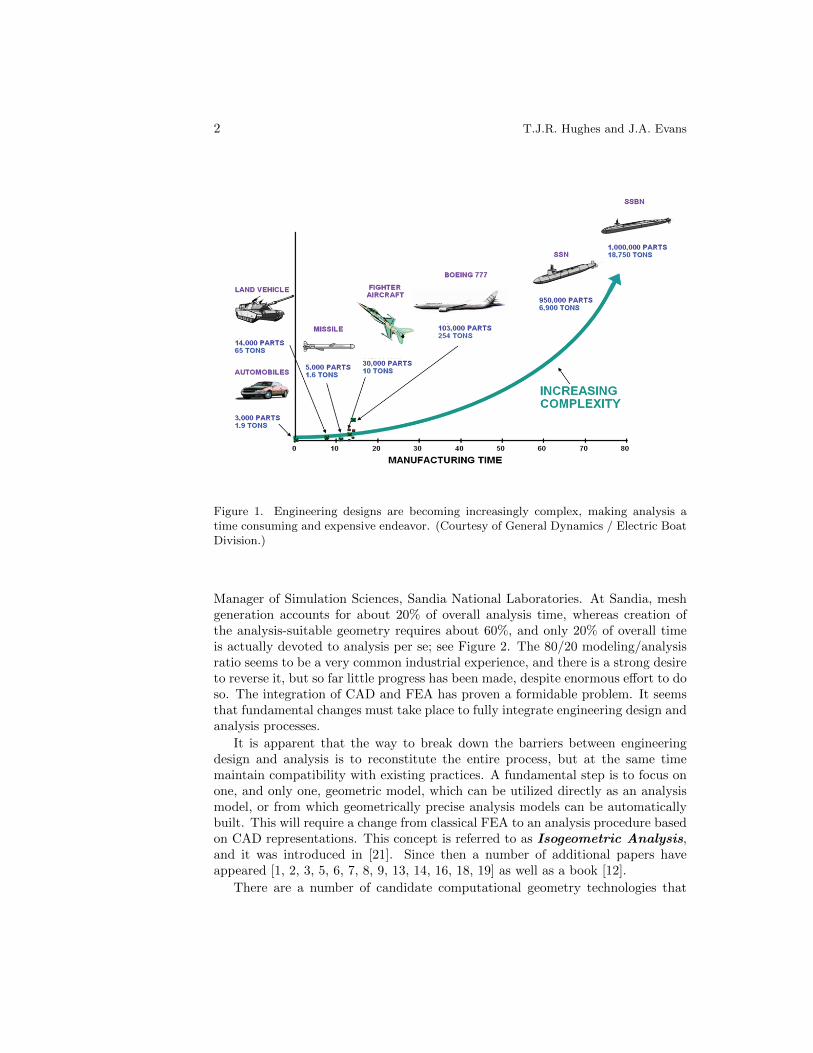
Designers generate CAD (Computer Aided Design) files and these must be trans-lated into analysis-suitable geometries, meshed and input to large-scale finite el-ement analysis (FEA) codes. This task is far from trivial and for complex engi-neering designs is now estimated to take over 80% of the overall analysis time, andengineering designs are becoming increasingly more complex; see Figure 1. Forexample, presently, a typical automobile consists of about 3,000 parts, a fighter jetover 30,000, the Boeing 777 over 100,000, and a modern nuclear submarine over1,000,000. Engineering design and analysis are not separate endeavors. Design ofsophisticated engineering systems is based on a wide range of computational anal-ysis and simulation methods, such as structural mechanics, fluid dynamics, acous-tics, electromagnetics, heat transfer, etc. Design speaks to analysis, and analysisspeaks to design. However, analysis-suitable models are not automatically cre-ated or readily meshed from CAD geometry. Although not always appreciated inthe academic analysis community, model generation is much more involved thansimply generating a mesh. There are many time consuming, preparatory stepsinvolved. And one mesh is no longer enough. According to Steve Gordon, Princi-pal Engineer, General Dynamics Electric Boat Corporation, “We find that today’sbottleneck in CAD-CAE integration is not only automated mesh generation, it lieswith efficient creation of appropriate ‘simulation-specific’ geometry.” (In the com-mercial sector analysis is usually referred to as CAE, which stands for ComputerAided Engineering.) The anatomy of the process has been studied by Ted Blacker,

2 T.J.R. Hughes and J.A. Evans

Figure 1. Engineering designs are becoming increasingly complex, making analysis atime consuming and expensive endeavor. (Courtesy of General Dynamics / Electric BoatDivision.)

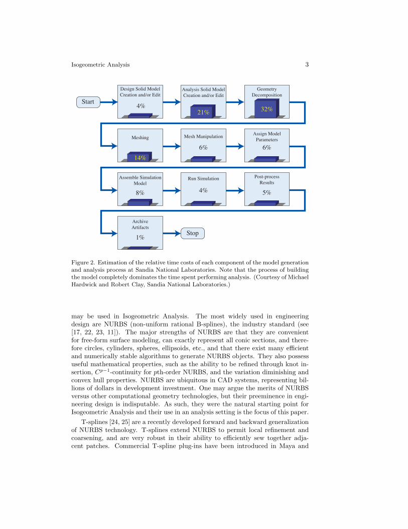
Manager of Simulation Sciences, Sandia National Laboratories. At Sandia, meshgeneration accounts for about 20% of overall analysis time, whereas creation ofthe analysis-suitable geometry requires about 60%, and only 20% of overall timeis actually devoted to analysis per se; see Figure 2. The 80/20 modeling/analysisratio seems to be a very common industrial experience, and there is a strong desireto reverse it, but so far little progress has been made, despite enormous effort to doso. The integration of CAD and FEA has proven a formidable problem. It seemsthat fundamental changes must take place to fully integrate engineering design andanalysis processes.

It is apparent that the way to break down the barriers between engineeringdesign and analysis is to reconstitute the entire process, but at the same timemaintain compatibility with existing practices. A fundamental step is to focus onone, and only one, geometric model, which can be utilized directly as an analysismodel, or from which geometrically precise analysis models can be automaticallybuilt. This will require a change from classical FEA to an analysis procedure basedon CAD representations. This concept is referred to as Isogeometric Analysis,and it was introduced in [21]. Since then a number of additional papers haveappeared [1, 2, 3, 5, 6, 7, 8, 9, 13, 14, 16, 18, 19] as well as a book [12].

There are a number of candidate computational geometry technologies that

Isogeometric Analysis 3

Design Solid ModelCreation and/or Edit

4%

GeometryDecomposition

32%

Analysis Solid ModelCreation and/or Edit

21%

Meshing

14%

Mesh Manipulation

6%

Assign ModelParameters

6%

Assemble SimulationModel

8%

Run Simulation

4%

Post-processResults

5%

ArchiveArtifacts

1%

Start

Stop

Figure 2. Estimation of the relative time costs of each component of the model generationand analysis process at Sandia National Laboratories. Note that the process of buildingthe model completely dominates the time spent performing analysis. (Courtesy of MichaelHardwick and Robert Clay, Sandia National Laboratories.)

may be used in Isogeometric Analysis. The most widely used in engineeringdesign are NURBS (non-uniform rational B-splines), the industry standard (see[17, 22, 23, 11]). The major strengths of NURBS are that they are convenientfor free-form surface modeling, can exactly represent all conic sections, and there-fore circles, cylinders, spheres, ellipsoids, etc., and that there exist many efficientand numerically stable algorithms to generate NURBS objects. They also possessuseful mathematical properties, such as the ability to be refined through knot in-sertion, Cp−1-continuity for pth-order NURBS, and the variation diminishing andconvex hull properties. NURBS are ubiquitous in CAD systems, representing bil-lions of dollars in development investment. One may argue the merits of NURBSversus other computational geometry technologies, but their preeminence in engi-neering design is indisputable. As such, they were the natural starting point forIsogeometric Analysis and their use in an analysis setting is the focus of this paper.

T-splines [24, 25] are a recently developed forward and backward generalizationof NURBS technology. T-splines extend NURBS to permit local refinement andcoarsening, and are very robust in their ability to efficiently sew together adja-cent patches. Commercial T-spline plug-ins have been introduced in Maya and


Rhino, two NURBS-based design systems (see references [27] and [28]). Initiatoryinvestigations of T-splines in an Isogeometric Analysis context have been under-taken by [4] and [15]. These works point to a promising future for T-splines as anisogeometric technology.

2. Basics of NURBS-based Isogeometric Analysis

In FEA there is one notion of a mesh and one notion of an element, but an elementhas two representations, one in the parent domain and one in the physical space.Elements are usually defined by their nodal coordinates and the degrees-of-freedomare usually the values of the basis functions at the nodes. Finite element basisfunctions are typically interpolatory and may take on positive and negative values.Finite element basis functions are often referred to as “interpolation functions,” or“shape functions.” See [20] for a discussion of the basic concepts.

In NURBS, the basis functions are usually not interpolatory. There are twonotions of meshes, the control mesh1 and the physical mesh. The control pointsdefine the control mesh, and the control mesh interpolates the control points. Thecontrol mesh consists of multilinear elements, in two dimensions they are bilinearquadrilateral elements, and in three dimensions they are trilinear hexahedra. Thecontrol mesh does not conform to the actual geometry. Rather, it is like a scaffoldthat controls the geometry. The control mesh has the look of a typical finiteelement mesh of multilinear elements. The control variables are the degrees-of-freedom and they are located at the control points. They may be thought of as“generalized coordinates.” Control elements may be degenerated to more primitiveshapes, such as triangles and tetrahedra. The control mesh may also be severelydistorted and even inverted to an extent, while at the same time, for sufficientlysmooth NURBS, the physical geometry may still remain valid (in contrast withfinite elements).

The physical mesh is a decomposition of the actual geometry. There are twonotions of elements in the physical mesh, the patch and the knot span. The patchmay be thought of as a macro-element or subdomain. Most geometries utilizedfor academic test cases can be modeled with a single patch. Each patch hastwo representations, one in a parent domain and one in physical space. In two-dimensional topologies, a patch is a rectangle in the parent domain representation.In three dimensions it is a cuboid.

Each patch can be decomposed into knot spans. Knots are points, lines, andsurfaces in one-, two-, and three-dimensional topologies, respectively. Knot spansare bounded by knots. These define element domains where basis functions aresmooth (i.e., C∞). Across knots, basis functions will be Cp−m where p is thedegree2 of the polynomial and m is the multiplicity of the knot in question. Knot

1The control mesh is also known as the “control net,” the “control lattice,” and curiously the“control polygon” in the univariate case.

2There is a terminology conflict between the geometry and analysis communities. Geometerswill say a cubic polynomial has degree 3 and order 4. In geometry, order equals degree plus


0 1 2 3 4,4 50

1 N1,2N2,2

N3,2 N4,2 N5,2

N6,2

N7,2

N8,2

Figure 3. Quadratic B-spline basis functions for open, non-uniform knot vector Ξ =0, 0, 0, 1, 2, 3, 4, 4, 5, 5, 5.

spans are convenient for numerical quadrature. They may be thought of as micro-elements because they are the smallest entities we deal with. They also haverepresentations in both a parent domain and physical space. When we speak of“elements” without further description, we usually mean knot spans.

There is one other very important notion that is a key to understanding NURBS,the index space of a patch. It uniquely identifies each knot and discriminatesamong knots having multiplicity greater than one.

NURBS basis functions are the rational counterpart of standard B-spline basisfunctions. For a discussion of the construction of B-spline basis functions on theparent domain from preassigned knot vectors, see Chapter 2 of [12]. A quadraticexample is presented in Figure 3. B-spline basis functions exhibit many desirableproperties, including partition of unity, compact support, and point-wise positivity.Multi-dimensional basis functions are defined through a tensor product, and basisfunctions are defined in physical space through a push-forward, i.e. by consid-ering a composition with the inverse of the geometrical mapping. In IsogeometricAnalysis, the isoparametric concept is invoked. That is, the same basis is usedfor both geometry and analysis. Analogues of h- and p-refinement also exist inIsogeometric Analysis in the form of knot insertion and order elevation, and thereis a new refinement scheme called k-refinement. See Chapter 2.1.4 of [12].

See Table 2 for a summary of NURBS paraphernalia employed in IsogeometricAnalysis. A schematic illustration of the ideas is presented in Figure 4 for a NURBSsurface in R3. For more details on B-splines and NURBS, see [17, 22, 23, 11].

3. Boundary Value Problems

As an example of solving a differential equation posed over the domain definedby a NURBS geometry, let us consider Laplace’s equation. The goal is to find

one. Analysts will say a cubic polynomial is order three, and use the terms order and degreesynonymously. This is the convention we adhere to.


ξ1 ξ7ξ6ξ5ξ4ξ3ξ2

η1

η2

η3

η4

η5

η6

η7

η8

Index space

Ξ = ξ1,ξ2 ,ξ3,ξ4 ,ξ5 ,ξ6 ,ξ7 = 0, 0, 0, 1/2, 1, 1, 1

H = η1,η2 ,η3,η4 ,η5 ,η6 ,η7 ,η8 = 0, 0, 0, 1/3, 2/3, 1, 1, 1

Knot vectors

0 1

1

2/3

1/3

01/2

ξ

η

N1 N4N2 N3

M1

M2

M3

M4

M5

R2

-1 1-1

1

ξ

η

Parameterspace

Parentelement

0 11/2

Rij ξ,η( ) =wij Ni (ξ)M j (η)wi j Ni (ξ)M j (η)

i , j∑

ξ

η

Integration isperformed on theparent element1

2/3

1/3

0x

y

z

Control point Bij

R3

Control mesh

Physical mesh

Physical space

S ξ,η( ) = Bij Rij ξ,η( )i, j∑

Figure 4. Schematic illustration of NURBS paraphernalia for a one-patch surface model.Open knot vectors and quadratic C1-continuous basis functions are used. Complex multi-patch geometries may be constructed by assembling control meshes as in standard FEA.Also depicted are C1-quadratic (p = 2) basis functions determined by the knot vectors.Basis functions are multiplied by control points and summed to construct geometricalobjects, in this case a surface in R3. The procedure used to define basis functions fromknot vectors is described in detail in Chapter 2 of [12].


Index Space

Control Mesh Physical Mesh

Multilinear Control Elements Patches Knot Spans

Topology:

1D: Straight lines definedby two consecutivecontrol points

2D: Bilinear quadrilater-als defined by fourcontrol points

3D: Trilinear hexahedradefined by eight con-trol points

Patches: Images ofrectangular meshesin the parent domainmapped into the actualgeometry. Patchesmay be thought ofas macro-elements orsubdomains.

Topology of knots in theparent domain:

1D: Points

2D: Lines

3D: Planes

Topology:

1D: Curves

2D: Surfaces

3D: Volumes

Topology of knots in thephysical space:

1D: Points

2D: Curves

3D: Surfaces

Patches are decom-posed into knot spans,the smallest notion ofan element.

Topology of knotsspans, i.e., “elements”:

1D: Curved segmentsconnecting con-secutive knots

2D: Curved quadrilat-erals bounded byfour curves

3D: Curved hexahedrabounded by sixcurved surfaces

Table 1. NURBS paraphernalia in Isogeometric Analysis


u : Ω→ R such that

∆u+ f = 0 in Ω, (1a)

u = g on ΓD, (1b)

∇u · n = h on ΓN , (1c)

βu+∇u · n = r on ΓR, (1d)

where ΓD⋃

ΓN⋃

ΓR = Γ ≡ ∂Ω, ΓD⋂

ΓN⋂

ΓR = ∅, and n is the unit outwardnormal vector ∂Ω. The functions f : Ω → R, g : ΓD → R, h : ΓN → R, andr : ΓR → R are all given, as is the constant β. Equation (1) constitutes the strongform of the boundary value problem (BVP). The boundary conditions given in(1b), (1c), and (1d) represent the three major types of boundary conditions oneis likely to encounter. These are Dirichlet conditions, Neumann conditions, andRobin conditions, respectively.

For a sufficiently smooth domain, and under certain restrictions on g, h, and r,a unique solution u satisfying (1) is known to exist, but an analytical expression willusually be impossible to obtain. However, we may seek an approximate solutionof the form

uh =∑A

dANA (2)

where NA is a basis function and dA is an unknown to be determined. We generi-cally refer to techniques for doing so as numerical methods. Different numericalmethods are simply different techniques for finding dA such that uh ≈ u. We focushere on the Bubnov-Galerkin method that underlies most of modern FEA.

The technique begins by defining a weak, or variational, counterpart of (1). Todo so, we need to characterize two classes of functions. The first is to be composedof candidate, or trial solutions. From the outset, these functions will be requiredto satisfy the Dirichlet boundary condition of (1b).

To define the trial and weighting spaces formally, let us first define the spaceof square integrable functions on Ω. This space, called L2(Ω), is defined as thecollection of all functions u : Ω→ R such that∫

Ω

u2 dΩ < +∞. (3)

Let us consider a multi-index ααα ∈ Nd where d is the number of spatial di-mensions in the space. For ααα = α1, . . . , αd, we define |ααα| =

∑di=1 αi. We now

have a concise way to represent derivative operators. Let Dααα = Dα11 Dα2

2 . . . Dαdd ,

where Dji = ∂j

∂xji. So that certain expressions to be employed in the formulation

make sense, we shall require that the derivatives of the trial solutions be square-integrable. Such a function is said to be in the Sobolev space H1(Ω), which ischaracterized by

H1(Ω) = u|Dαααu ∈ L2(Ω), |ααα| ≤ 1. (4)

We may now define the collection of trial solutions, denoted by S, as all ofthe function which have square-integrable derivatives and that also satisfy

u|ΓD = g. (5)


This is written asS = u | u ∈ H1(Ω), u|ΓD = g. (6)

The second collection of functions in which we are interested is called theweighting functions. This collection is very similar to the trial functions, exceptthat we have the homogeneous counterpart of the Dirichlet boundary condition.That is, the weighting functions are denoted by a set V defined by

V = w | w ∈ H1(Ω), w|ΓD = 0. (7)

We may now obtain a variational statement of the BVP by multiplying (1a)by an arbitrary test function w ∈ V and integrating by parts, incorporating (1c)and (1d) as needed. The resulting weak form of the problem is now: Given f , g,h, and r, find u ∈ S such that for all w ∈ V∫

Ω

∇w · ∇u dΩ + β

∫ΓR

wudΓ

=

∫Ω

wf dΩ +

∫ΓN

whdΓ +

∫ΓR

wr dΓ. (8)

This weak form may be rewritten as

a(w, u) = L(w) (9)

where

a(w, u) =

∫Ω

∇w · ∇u dΩ + β

∫ΓR

wudΓ, (10)

and

L(w) =

∫Ω

wf dΩ +

∫ΓN

whdΓ +

∫ΓR

wr dΓ. (11)

This concise notation, or variants thereof, is quite common in the finite elementliterature. For problems other than the Laplace equation, the details vary, but thebasic form remains. It captures the essential mathematical features of the varia-tional method (as well as suggesting features of a finite element implementation)that are more general than the details of the equation itself.

The solution to (8), or equivalently (9), is called a weak solution. Underappropriate regularity assumptions, it can be shown that the weak solution andthe strong solution of (1) are equivalent; see [20].

The Bubnov-Galerkin method, abbreviated as Galerkin’s method, consists ofconstructing finite-dimensional approximations of S and V, denoted Sh and Vh,respectively. Strictly speaking, these will be subsets such that

Sh ⊂ S, (12)

Vh ⊂ V. (13)

Furthermore, these will be associated with subsets of the space spanned by theisoparametric basis. In Isogeometric Analysis, these spaces consist of mappedNURBS functions.


We can further characterize Sh by recognizing that if we have a given functiongh ∈ Sh such that gh|ΓD = g, then for every uh ∈ Sh, there exists a unique vh ∈ Vhsuch that

uh = vh + gh. (14)

We can now write a variational equation of the form of (9). The Galerkin form ofthe problem is: Given gh, h, and r, find uh = vh + gh, where vh ∈ Vh, such thatfor all wh in Vh

a(wh, uh) = L(wh). (15)

Recalling (14) and the bilinearity of a(·, ·), we can rewrite (15) as

a(wh, vh) = L(wh)− a(wh, gh). (16)

In this latter form, the unknown information is on the left-hand-side, while every-thing on the right-hand-side is given, as before.

The finite-dimensional nature of the function spaces used in Galerkin’s methodleads to a coupled system of linear algebraic equations. Let the solution spaceconsist of all linear combinations of a given set of NURBS functions NA : Ω→ R,where A = 1, . . . , nnp. Without loss of generality, we may assume a numbering forthese functions such that there exists an integer neq < nnp such that

NA|ΓD = 0 ∀A = 1, . . . , neq. (17)

Thus, for all wh ∈ Vh, there exist constants cA, A = 1, . . . , neq such that

wh =

neq∑A=1

NAcA. (18)

Furthermore, the function gh (frequently called a “lifting”) is given similarly bycoefficients gA, A = 1, . . . , nnp. In practice, we will always choose gh such thatg1 = . . . = gneq = 0 as they have no effect on its value on ΓD, and so

gh =

nnp∑A=neq+1

NAgA. (19)

Finally, recalling again (14), for any uh ∈ Sh there exist dA, A = 1, . . . , neq suchthat

uh =

neq∑A=1

NAdA +

nnp∑B=neq+1

NBgB =

neq∑A=1

NAdA + gh. (20)

Proceeding to define

KAB = a(NA, NB), (21)

FA = L(NA)− a(NA, gh), (22)


and

K = [KAB ], (23)

F = FA, (24)

d = dA, (25)

for A,B = 1 . . . , neq, we can rewrite (16) as the matrix problem

Kd = F. (26)

The matrix K is commonly referred to as the stiffness matrix, and F and d arereferred to as the force and displacement vectors, respectively.

It is important to note that K is a sparse matrix. This is a result of the fact thatthe support of each basis function is highly localized. Thus, for many combinationsof A and B in the neq × neq global stiffness matrix, KAB = a(NA, NB) = 0. Wecan take advantage of this fact in order to reduce the amount of work necessaryin building and solving the algebraic system. Things are further simplified byemploying Gaussian quadrature to perform integrations. This process is detailedin Section 3.3.1 of [12]. Even though the NURBS functions are not necessarilypolynomials, Gaussian quadrature seems to be very effective for integrating them.Though this approach to integration is only approximate, it is important to notethat integrating the classical polynomial functions by quadrature on elements withcurved sides is only an approximation as well.

Once Galerkin’s method has been applied and an approximation, uh, has beenobtained, it is fair to inquire as to just how good of an approximation it is. Resultsfor classical FEA and Isogeometric Analysis are discussed in the next session. Itturns out that, for elliptic problems such as the one considered in this section, thesolution is optimal in a very natural sense; see Chapter 4 of [20].

4. Error Estimates for NURBS

4.1. FEA. Well established a priori approximation results exist for classicalfinite elements applied to elliptic problems (see, for example, the classic text by[10]). The Sobolev space of order r is defined by

Hr(Ω) = u|Dαααu ∈ L2(Ω), |ααα| ≤ r. (27)

The norm associated with Hr(Ω) is given by

‖u‖2r =∑|ααα|≤r

∫Ω

(Dαααu) · (Dαααu) dx. (28)

In classical FEA, the fundamental error estimate for the elliptic boundary valueproblem, expressed as a bound on the difference between the exact solution, u,and the FEA solution, uh, takes the form

‖u− uh‖m ≤ Chβ‖u‖r, (29)


where ‖ · ‖m and ‖ · ‖r are the norms corresponding to Sobolev spaces Hm(Ω) andHr(Ω), respectively, h is a characteristic length scale related to the size of theelements in the mesh, β = min(p+ 1−m, r −m) where p is the polynomial orderof the basis, and C is a constant that does not depend on u or h.

The term of interest in (29) is hβ . The mesh parameter, h, can be defined inseveral ways, with the specific definition affecting C. A fairly general definition isthe diameter of the smallest circle (in two dimensions) or sphere (in three dimen-sions) that is large enough to circumscribe any element in the mesh. The order ofconvergence, β, expresses how the error changes under refinement of the mesh.In particular, if we use h-refinement to bisect each of the elements in the mesh(i.e., h is replaced with h/2), we would expect the error to decrease by a factor of(1/2)β .

4.2. NURBS. The extremely technical details of the process of obtaining aresult analogous to (29) for NURBS can be found in [3]. Here we present the basicideas, but encourage the interested reader to consult the original publication.

For classical FEA polynomials, the result in (29) is obtained by first establishingthe interpolation properties of the basis. Let Πm be the projection operator fromHm(Ω) into the space spanned by the FEA basis. Then the optimal interpolate isthe function

ηh = Πmu (30)

such that‖u− ηh‖m ≤ ‖u− vh‖m ∀vh ∈ Sh, (31)

where Sh is the finite element space. To establish just how good this optimalapproximation is (i.e., to determine how can ‖u− ηh‖m be bounded), we obtain abound on each element, and then sum over all of the elements to get a global result.With this interpolation result in hand, the second step in the process is to relatethe result of the Galerkin finite element method, uh, to the optimal interpolate, ηh.In particular, it can be shown that the order of convergence of the finite elementsolution is the same as for the optimal interpolate. Taken together, these tworesults yield the the bound (29), which states that (up to a constant) Galerkin’smethod gives us the optimal result.

When we seek an analogous result for NURBS, we face several difficulties.The first is that the approximation properties of this rational basis are harder todetermine than are those of a standard polynomial basis. In particular, note thatthe weights are determined by the geometry and so are out of our control whenwe attempt to approximate a field over that geometry and cannot be adjusted toimprove the result. The second difficulty originates from the large support of thespline functions. Standard interpolation estimates seek to find a best fit withineach element and then aggregate these results to obtain an approximation over theentire domain. This is non-trivial with the spline functions because the support ofeach function spans several elements, and so we cannot determine optimal valuesfor the control variables by looking at each element individually. The issue isfurther complicated by the possibility of differing levels of continuity (and thusdiffering sizes of the the supports of the functions) throughout the domain.


To overcome the fact that the basis is rational rather than polynomial, we firstnote that the parameter space Ω can be considered to be the unit cube [0, 1]d. Nogenerality is lost in this assumption as dividing a knot vector by a constant oradding a constant does not change the resulting physical domain in any way. Letus first denote a NURBS basis function as:

Ri(ξ) =Ni(ξ)wiW (ξ)

, (32)

with

W (ξ) =

n∑i=1

Ni(ξ)wi (33)

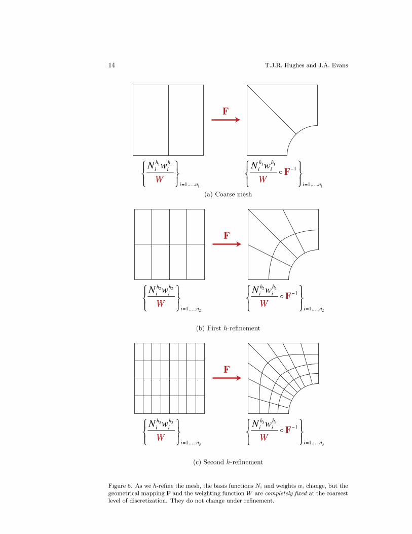
where Ni is the corresponding B-spline basis function. The important thing to noteis that the weighting function3, W (ξ), does not change as we h-refine the mesh(it does not change under p-refinement either, though this is not the case we areinterested in at present). While both the weights and the basis functions change,they do so in such a way as to leave W (ξ) unaltered. Similarly, the geometricalmapping from the parameter space into the physical space, F : Ω → Ω, does notchange as we insert new knot values. See Figure 5. It remains exactly the sameat all levels of refinement. To take advantage of this fact, we consider the functionwe wish to approximate, u : Ω → R`. As the geometrical mapping is one-to-one,we can pull this back to the parametric domain to define u = u F−1 : Ω → R`.Lastly, we can lift the image of the function using the weighting function to defineu = Wu,W : Ω → R`+1. Recalling that we obtain the rational basis in Rd bya projective transformation (equivalent to dividing by W ) of a B-spline basis inRd+1, we see that the ability of the rational NURBS basis to approximate u on Ωis intimately related to the ability of the underlying B-spline basis to approximateu on Ω. Thus we have reduced the problem of understanding a rational basis on ageneral domain to that of understanding a polynomial basis on the unit cube.

The second hurdle is more technical. The fact that each function has supportover many elements and that the continuity across the various element boundariescan vary from one boundary to the next greatly complicates matters comparedwith the classical case. [3] address this difficulty by proving approximation resultsin so-called “bent” Sobolev spaces in which the continuity varies throughout thedomain. A sequence of lemmas is established leading up to an approximation resultthat includes not only the norm in these bent Sobolev spaces of the function u beingapproximated, but also the gradient of the mapping, ∇F. This last term presentsno problem because, as already discussed, it does not change as the mesh is refined,and thus does not affect the rate of convergence. The resulting approximationresult is: Let k and l be integer indices such that 0 ≤ k ≤ l ≤ p + 1, and letu ∈ H l(Ω); then

nel∑e=1

|u−Πku|2Hk(Ωe) ≤ Cnel∑e=1

h2(l−k)e

l∑i=0

‖∇F‖2(i−l)L∞(F−1(Ωe))|u|

2Hi(Ωe). (34)

3Do not confuse this use of the term “weighting function” with the unrelated use of the sameterminology in Galerkin’s method.


F

Nih1wi

h1

W⎧⎨⎩

⎫⎬⎭i=1,K,n1

Nih1wi

h1

Wo F−1⎧

⎨⎩

⎫⎬⎭i=1,K,n1

(a) Coarse mesh

F

Nih2wi

h2

W⎧⎨⎩

⎫⎬⎭i=1,K,n2

Nih2wi

h2

Wo F−1⎧

⎨⎩

⎫⎬⎭i=1,K,n2

(b) First h-refinement

F

Nih3wi

h3

W⎧⎨⎩

⎫⎬⎭i=1,K,n3

Nih3wi

h3

Wo F−1⎧

⎨⎩

⎫⎬⎭i=1,K,n3

(c) Second h-refinement

Figure 5. As we h-refine the mesh, the basis functions Ni and weights wi change, but thegeometrical mapping F and the weighting function W are completely fixed at the coarsestlevel of discretization. They do not change under refinement.


The constant C depends on p and the shape (but not size) of the domain Ω, aswell as the shape regularity of the mesh. The factors involving the gradient of themapping render the estimate dimensionally consistent.

Finally, with the approximation result of (34) in hand, establishing the mannerin which the Isogeometric Analysis solution, uh, relates to the optimal interpolate,ηh, proceeds exactly as in the classical case. Combining these results yields thedesired result: The Isogeometric Analysis solution obtained using NURBS of orderp has the same order of convergence as we would expect in a classical FEA settingusing classical basis functions with a polynomial order of p. This is an exceptionallystrong result as it is independent of the order of continuity that the mesh possesses.That is, bisecting all of the elements in an FEA mesh (thus cutting the mesh pa-rameter from h to h/2) requires the introduction of many more degrees-of-freedomthan does bisection of the same number of NURBS elements while maintainingp− 1 continuity (see Section 2.1.4 of [12]). This means that NURBS can convergeat the same rate as FEA polynomials, while remaining much more efficient.

4.3. Explicit h-k-p-estimates for NURBS. The theoretical study of[3] is continued in [6], focusing on the relation between the degree p and the globalregularity k of a NURBS space and its approximation properties. Indeed, errorestimates that are explicit in terms of the mesh-size h, and p, k are obtained. Theapproach is restricted to Ck−1 approximations, with 2k − 1 ≤ p. The interestingcase of higher regularity, up to k = p, is still open. However, the results give anindication of the role of the smoothness k and offer a first mathematical justifica-tion of the potential of Isogeometric Analysis based on globally smooth NURBS.The main result, in a simplified form and in the two-dimensional setting, is thefollowing: let v be a function to be approximated. Then there exists a NURBSapproximation Πv such that

|v −Πv|H`(Ωe) ≤ C(p− k + 1)−(σ−`)hσ−`e ‖v‖Hσ(Ωe) (35)

where Ωe is a mesh element of diameter he in the NURBS physical domain Ω,2k ≤ σ ≤ p + 1, and ` ≤ k. In [6], different asymptotic regimes are studied. Inparticular, when v is smooth, the strong advantage of higher k is shown.

5. Vibrations

The study of structural vibrations or, more specifically, of eigenvalue problemsallows us to examine in more detail the approximation properties of the smoothNURBS functions independently of any geometrical considerations. In general,spectrum analysis is the term applied to the study of how numerically com-puted natural frequencies, ωhn, compare with the analytically computed naturalfrequencies, ωn. We will see that, for a given number of degrees-of-freedom andbandwidth, the use of NURBS results in dramatically improved accuracy in spec-tral calculations over classical FEA.


Let us begin by considering one of the simplest vibrational model problemsin one dimension: the longitudinal vibrations of an elastic rod. If we considerthe domain Ω = (0, L) ⊂ R, there is no longer an issue of geometrical accuracy.FEA basis functions and NURBS4 are equally capable of representing this domainexactly, and so the quality of the results will depend entirely on the approximationproperties of the basis.

To understand the formulation of the eigenproblem representing the longitudi-nal vibrations of a “fixed-fixed” elastic rod, let us begin by considering the elas-todynamics equation from which it is derived. The behavior of the rod, which isassumed to move only in the longitudinal direction, is governed by the equationsof linear elasticity combined with Newton’s second law, resulting in

(Eu,x),x − ρu,tt = 0 in Ω× (0, T ), (36a)

u = 0 on Γ× (0, T ), (36b)

where Ω = (0, L), ρ : (0, L) → R is the density per unit length of the rod, E :(0, L)→ R is Young’s modulus, and the “fixed-fixed” condition (36b) ensures thatthe ends of the rod do not move. For an actual dynamics problem, we would needto augment (36) with appropriate initial conditions of the form

u(x, 0) = u0(x), (37)

u,t(x, 0) = v0(x). (38)

At present, however, we are not interested in the transient behavior of the rod.Instead, we are interested in the natural frequencies and modes in which the rodvibrates. We obtain these by separation of variables. In a slight abuse of notation,we assume u(x, t) to have the form

u(x, t) = u(x)eiωt, (39)

where u(x) is a function of only the spatial variable, x, while i =√−1, and ω

is the natural frequency. Inserting (39) into (36a) and dividing by the commonexponential term results in the eigenproblem we are seeking:

(Eu,x),x + ω2ρu = 0 in Ω, (40a)

u = 0 on Γ. (40b)

Equation (40) constitutes an eigenproblem for the rod. The nontrivial solutionsare countably infinite. That is, for k = 1, 2, . . . ,∞, there is an eigenvalue λk =(ωk)2 and corresponding eigenfunction u(k) satisfying (40). Furthermore, 0 < λ1 ≤λ2 ≤ . . ., and the eigenfunctions are orthogonal. Though the eigenfunctions areonly defined up to a multiplicative constant, we can remove the arbitrariness byaugmenting the orthogonality condition to include normality.

Following the now familiar process, we multiply (40a) by a test function w andintegrate by parts to obtain the weak form of the equation: Find all eigenpairsu, λ, u ∈ S, λ = ω2 ∈ R+, such that for all w ∈ V

a(w, u)− ω2(w, ρu) = 0, (41)

4In this simple domain, the NURBS reduce to the special case of B-splines.


where

a(w, u) =

L∫0

w,xEu,x dx, (42)

(w, ρu) =

L∫0

wρudx. (43)

Note that, due to the homogeneous boundary conditions, S = V = H10 (0, L) =

u ∈ H1(0, L)|u(0) = u(L) = 0.The Galerkin formulation is obtained by restricting ourselves to finite-dimensional

subspaces Sh ⊂ S in the usual way. That is, w and u in (41) will be replaced byfinite dimensional approximations wh and uh of the form

wh =

neq∑A=1

NAdA and uh =

neq∑B=1

NBcB , (44)

respectively. The resulting eigenpairs will contain approximations of both naturalmodes uh(k) and the natural frequencies ωhk . The problem becomes: Find all ωh ∈R+ and uh ∈ Sh such that for all wh ∈ Vh

a(wh, uh)− (ωh)2(wh, ρuh) = 0. (45)

Substituting the shape-function expansions for wh and uh in (45) gives rise to amatrix eigenvalue problem: Find natural frequency ωhk ∈ R+ and eigenvector ΨΨΨk,k = 1, . . . , neq, such that (

K− (ωhk )2M)

ΨΨΨk = 0, (46)

where

K = [KAB ], (47)

M = [MAB ], (48)

with

KAB = a(NA, NB), (49)

MAB = (NA, ρNB), (50)

and ΨΨΨk is the vector of control variables corresponding to uh(k).As before, we refer to K as the stiffness matrix. The new object, M, is

the mass matrix. Noting that ρ > 0, and that the NURBS basis functions arepointwise non-negative, we see from (43) that every entry in the mass matrix isalso non-negative. This claim cannot be made for standard finite elements.

Let us consider the case where ρ, E, and L are each taken to be 1. Analytically,(40a) can be solved to obtain ωn = nπ for n = 1, . . . ,∞. We can assess the qualityof the numerical method by comparing the ratio of the computed modes, ωhn, with


the analytical result. That is, (ωhn/ωn) = 1 indicates that the numerical frequencyis identical to the analytical result. In practice, the discrete frequencies will alwaysobey the relationship

ωn ≤ ωhn for n = 1, . . . , neq, (51)

and so we expect the ratio (ωhn/ωn) to be greater than 1 (see, e.g., [26]), with largervalues indicating decreased accuracy.

Figure 6 shows a comparison of k-method (Cp−1 pth-order NURBS) and p-method (C0 pth-order finite elements) numerical spectra for p = 1, ..., 4 (we recallthat for p = 1 the two methods coincide). Here, the superiority of the isogeometricapproach is evident, as one can see that for C0 finite elements the higher modesdiverge with p. This negative result shows that even higher-order finite elementshave no approximability for higher modes in vibration analysis, and possibly ex-plains the fragility of higher-order finite element methods in nonlinear and dynamicapplications in which higher modes necessarily participate. In contrast, the entireNURBS spectrum converges for all modes. This dramatic result is all the morecompelling when we recall that the result is independent of the geometry in thisone-dimensional setting. Results such as these can be understood from a morefundamental functional analysis perspective through the notion of Kolmogorovn-widths.

0 0.1 0.2 0.3 0.4 0.5 0.6 0.7 0.8 0.9 11

1.1

1.2

1.3

1.4

1.5

1.6

n/N

FEM

NURBS

p

p

k−method, p=2k−method, p=3k−method, p=4p−method, p=2p−method, p=3p−method, p=4p=1

ωnh

/ωn

Figure 6. Longitudinal vibrations of an elastic rod. Comparison of k-method and p-method numerical spectra.


6. Kolmogorov n-widths

The approximation result (34) is a basic tool for proving convergence of NURBSto the solution of partial differential equations with h-refined meshes (see [3] forexamples). Note that the continuity of the basis functions does not explicitlyappear in (34). Consequently, the order of convergence in (34) depends only onthe order of the basis functions employed. However, the results of eigenvaluecalculations indicate that there is a dramatic difference between C0- and Cp−1-continuous pth-order basis functions (see, e.g., Figure 6). In Figure 6, as p isincreased, the upper part of the spectrum diverges for C0-continuous classical finiteelements whereas it converges for Cp−1-continuous NURBS (i.e., B-splines in thiscase). This phenomenon is not revealed by standard approximation theory resultsof the form (34). Consequently, we much conclude that there is a lot of informationhiding in the so-called “constant” C in (34). Indeed, the refined approximationresult (35) illustrates an explicit dependence of the constant on polynomial orderand continuity. However, the result is quite limited in its application as it isrestricted to Ck−1 approximations, with 2k − 1 ≤ p.

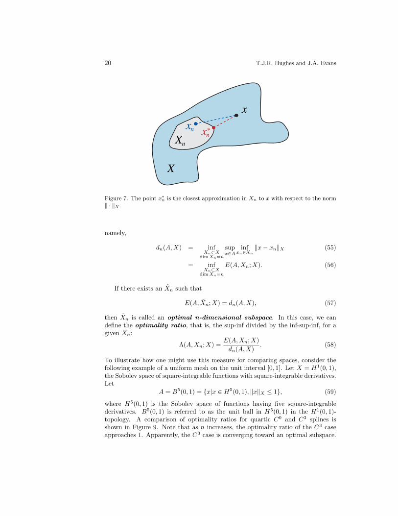
It would be desirable to develop a mathematical framework that revealed be-havior like that seen in Figures 6 from the outset. The concept of Kolmogorovn-widths seems to hold the potential to do so. A sketch of some of the main ideasfollows: Let X be a normed, linear space, equipped with norm ‖ · ‖X . In the casesof primary interest here, X would be a Sobolev space. Let Xn be an n-dimensionalsubspace of X. Assume we wish to approximate a given x ∈ A ⊂ X, where A is asubset of X, with a member xn ∈ Xn. We define the distance between x and Xn

as

E(x,Xn;X) = infxn∈Xn

‖x− xn‖X , (52)

where inf stands for infimum (see Figure 7). If there exists an x∗n such that

‖x− x∗n‖X = E(x,Xn;X) (53)

then x∗n is called the best approximation of x.

Now we assume we are interested in approximating all x ∈ A. For each x ∈ A,the best we can do is expressed by (53). The question we wish to have answeredis, for which x ∈ A do we get the worst best-approximation? In other words, forwhich x ∈ A is infxn∈Xn ‖x−xn‖X the largest? The idea is to anticipate situationssuch as those depicted in Figures 6. The worst best-approximation is obtained bycomputing the supremum of (53) over all x ∈ A; we define the deviation, or“sup-inf,” as

E(A,Xn;X) = supx∈A

infxn∈Xn

‖x− xn‖X . (54)

See Figure 8 for a schematic illustration. Sup-inf’s are useful for comparing theapproximation quality of different finite element subspaces, such as C0 and Cp−1

splines, but prior to that we might ask what is the best n-dimensional subspace forapproximating A? This is given by the Kolmogorov n-width, or “inf-sup-inf,”


X

Xn

xxn xn

∗

Figure 7. The point x∗n is the closest approximation in Xn to x with respect to the norm

‖ · ‖X .

namely,

dn(A,X) = infXn⊂X

dimXn=n

supx∈A

infxn∈Xn

‖x− xn‖X (55)

= infXn⊂X

dimXn=n

E(A,Xn;X). (56)

If there exists an Xn such that

E(A, Xn;X) = dn(A,X), (57)

then Xn is called an optimal n-dimensional subspace. In this case, we candefine the optimality ratio, that is, the sup-inf divided by the inf-sup-inf, for agiven Xn:

Λ(A,Xn;X) =E(A,Xn;X)

dn(A,X). (58)

To illustrate how one might use this measure for comparing spaces, consider thefollowing example of a uniform mesh on the unit interval [0, 1]. Let X = H1(0, 1),the Sobolev space of square-integrable functions with square-integrable derivatives.Let

A = B5(0, 1) = x|x ∈ H5(0, 1), ‖x‖X ≤ 1, (59)

where H5(0, 1) is the Sobolev space of functions having five square-integrablederivatives. B5(0, 1) is referred to as the unit ball in H5(0, 1) in the H1(0, 1)-topology. A comparison of optimality ratios for quartic C0 and C3 splines isshown in Figure 9. Note that as n increases, the optimality ratio of the C3 caseapproaches 1. Apparently, the C3 case is converging toward an optimal subspace.


X

Xn

Axn

x

xn∗

x∗

Figure 8. The distance between subspaces Xn and A is determined by the “worst-casescenario.” That is, if the distance between point x∗ ∈ A and its best approximationx∗n ∈ Xn is the supremum over all such best-fit pairs, then ‖x∗ − x∗

n‖X defines thedistance between Xn and A.

In contrast, in the C0 case, the optimality ratio converges to approximately 5.5,indicating that for each n there is at least one member of B5(0, 1) that is muchmore poorly approximated by C0 splines than C3 splines. This result seems to bequalitatively consistent with what we saw in Figures 6. Smooth spline bases, thatis the k-method, exhibit better behavior than classical C0 elements. For furtherresults and methodology used to compute them, see [16].

7. Smooth Isogeometric Discretizations

From the mathematical side, one of the most interesting aspects of Isogeomet-ric Analysis is the possibility to have smooth approximation fields. Smooth dis-crete spaces can be directly used with partial differential equations of order higherthan two. One interesting example is the stream-function approach to the Stokesproblem (see [1]). The solution of the Stokes variational equations is the pair5

(u, p) ∈ (H1D(Ω))2 × L2(Ω) such that

∫Ω

grad (u) : grad (v) +

∫Ω

p divv =

∫Ω

f · v ∀v ∈ H1D(Ω)

∫Ω

q divu = 0 ∀q ∈ L2(Ω),

(60)

5Here p is the pressure instead of the degree.


0 10 20 30 40 501

2

3

4

5

6

Number of degrees-of-freedom

(B5 (0

,1),X

n;H1 (0

,1))

C 0 FEAk method

Figure 9. The optimality ratio for approximating the H5 unit ball in H1 using quartic(p = 4) elements. As the number of degrees-of-freedom increases, the optimality ratio ofC0 FEA functions diverges, while the optimality ratio of C3-continuous splines convergestoward 1.

where H1D(Ω) is the Sobolev space of H1 functions vanishing on ΓD ⊂ ∂Ω. For

two-dimensional problems, the divergence-free field u can be represented as thecurl of a potential, the so called stream function, that is u = curlψ. Sincediv ( curlψ) = 0, one can replace (60) with∫

Ω

grad ( curlψ) : grad ( curlφ) =

∫Ω

f · curlφ ∀φ ∈ H2(Ω) + boundary conditions.

(61)The advantage of the above formulation is that at the discrete level, replacingH2(Ω) with a suitable NURBS space with at least global C1-continuity, one obtainsan approximation uh = curlψh which is exactly divergence-free.

The application of this approach to a more realistic problem is presented in[2] where the capability of various numerical methods to correctly reproduce thestability range of finite strain (nonlinear) problems in the incompressible regimeis studied. The stream-function isogeometric NURBS approach is applied to alinearized problem at each Newton step of the finite strain problem. This techniqueis able to sharply estimate the stability limits of the continuous problem in contrastwith various standard finite element methods. For example, a simple benchmarkproblem (an elastic incompressible square in plain strain under constant bodyload and clamped on three sides) is shown to be stable under compression up to aloading factor of 6.6, while various finite element methods show instabilities arounda loading factor of 1.


Another application area where smooth isogeometric discretizations can be uti-lized is the numerical simulation of phase-field models. Phase-field models providean alternative description for phase-transition phenomena. The key idea in thephase-field approach is to replace sharp interfaces by thin transition regions wherethe interfacial forces are smoothly distributed. The transition regions are part ofthe solution of the governing equations and, thus, front tracking is avoided. Phase-field models are typically characterized by higher-order differential operators andhence require smooth discretization techniques. Isogeometric Analysis has beenapplied to several phase-field models, including the Cahn-Hilliard equation [18]and the Navier-Stokes-Korteweg equations [19].

8. Vector Field Discretizations

An alternate approach to stream-functions which can also handle problems witha solenoidal constraint is the construction of B-splines or NURBS spaces whichfulfill the divergence-free property exactly. This is possible once again due to thesmoothness of isogeometric spaces, leading to an extension of classical Raviart-Thomas elements. These new discretizations can be used for a much wider class ofproblems (e.g., Stokes flow (60)) than classical Raviart-Thomas elements. In [9],smooth Raviart-Thomas B-splines and NURBS spaces are introduced and theirstudy is initiated. In [7], these spaces are used in the simulation of incompressiblefluid flows.

The mathematical structure behind the construction in [9] can be understoodin the framework of the Exterior Calculus. This has been done in [8] where a DeRham complex for B-spline spaces6 is constructed. Notably, there exist B-splinespaces Xi

h, i = 0, . . . , 3, of any degree and commuting projectors Πi, i = 0, . . . , 3such that

H1(Ω)grad−−−−→ H(curl; Ω)

curl−−−−→ H(div; Ω)div−−−−→ L2(Ω)

Π0

y Π1

y Π2

y Π3

yX0h

grad−−−−→ X1h

curl−−−−→ X2h

div−−−−→ X3h.

(62)

The above diagram paves the way to stable discretizations of a wide class of dif-ferential problems. For example, it provides spurious free smooth approximationof the Maxwell eigenproblem: find ω ∈ R, and u ∈ H(curl; Ω) , u 6= 0 such that∫

Ω

curl u · curl v = ω2

∫Ω

u · v ∀v ∈ H(curl; Ω) . (63)

For more details, see [8].

6Note that these are B-splines and not NURBS.


9. Conclusions

We have presented a brief mathematical introduction to Isogeometric Analysis,a new numerical methodology for solving partial differential equations (PDEs)that combines and synthesizes Computer Aided Design (CAD) and Finite Ele-ment Analysis (FEA) technologies. A main motivation of Isogeometric Analysis isto simplify the process of building FEA models from CAD files, a major bottle-neck in the overall engineering process. However, Isogeometric Analysis has alsoprovided new insights and methods for solving PDEs. By way of an example,we have shown that Isogeometric Analysis can provide more accurate solutionsof PDEs than classical C0-continuous finite elements. However, these differencesare not revealed by standard error analysis procedures utilizing functional analysistechniques in that they are rather insidiously hidden in “constants” in functionalanalysis inequalities. The example also illustrates a striking deficiency of classical,higher-order, C0-continuous finite elements, namely, the errors in higher modes di-verge with increasing polynomial order. This surprising result seems to explain theobserved fragility of these finite element spaces when used to obtain the solution ofnonlinear problems, which often involve higher-mode behavior. We also reportedon initial investigations using Kolmogorov n-widths to computationally determinethe relative merits of finite-dimensional approximating spaces. This amounts toan a priori approach capable of exposing deficiencies of approximating spaces forcomputing the solutions of PDEs.

We have also noted that the smooth, higher-order basis functions of Isogeo-metric Analysis open the way to efficiently solving higher-order PDEs on complexdomains. Problems of this kind, such as those representing multi-phase phenom-ena, have proven very difficult for standard FEA approaches. Finally, we brieflyreviewed recent mathematical work in Isogeometric Analysis devoted to the con-struction of smooth, divergence-free, approximating spaces for vector field prob-lems, and mentioned seminal functional analysis results that explicitly reveal theimprovements garnered by the smooth approximating spaces used in IsogeometricAnalysis.

Acknowledgements

We thank Lourenco Beirao de Veiga, Annalisa Buffa, and Giancarlo Sangalli forproviding us with a summary of their most recent results that we have includedherein. T.J.R. Hughes was partially supported by the Office of Naval Researchunder Contract Number N00014-08-0992 and by the National Science Foundationunder NSF Grant Number 0700204. J.A. Evans was partially supported by the De-partment of Energy Computational Science Graduate Fellowship, provided underGrant Number DE-FG02-97ER25308.


References

[1] F. Auricchio, L. Beirao de Veiga, A. Buffa, C. Lovadina, and A. Reali, A fully “locking-free” isogeometric approach for plane elasticity problems: A stream-function formula-tion, Computer Methods in Applied Mechanics and Engineering, 197, (2007) 160-172.

[2] F. Auricchio, L. Beirao de Veiga, C. Lovadina, and A. Reali, The importance of theexact satisfaction of the incompressibility constraint in nonlinear elasticity: MixedFEMs versus NURBS-based approximations, Computer Methods in Applied Mechan-ics and Engineering, 199, (2010) 314-323.

[3] Y. Bazilevs, L. Beirao de Veiga, J.A. Cottrell, T.J.R. Hughes, and G. Sangalli, Isoge-ometric analysis: approximation, stability, and error estimates for h-refined meshes,Mathematical Models and Methods in Applied Sciences, 16, (2006) 1031-1090.

[4] Y. Bazilevs, V.M. Calo, J.A. Cottrell, J.A. Evans, T.J.R. Hughes, S. Lipton, M.A.Scott, and T.W. Sederberg, Isogeometric analysis using T-splines, Computer Methodsin Applied Mechanics and Engineering, 199, (2010) 229-263.

[5] Y. Bazilevs, V.M. Calo, Y. Zhang, and T.J.R. Hughes, Isogeometric fluid-structureinteraction analysis with applications to arterial blood flow, Computational Mechanics,38, (2006) 310-322.

[6] L. Beirao da Veiga, A. Buffa, J. Rivas, and G. Sangalli, Some estimates for h-p-k-refinement in isogeometric analysis, Technical report, IMATI-CNR Preprint, 2009.

[7] A. Buffa, C. De Falco, and G. Sangalli, Isogeometric analysis: New stable elementsfor the Stokes equation, Technical Report, IMATI-CNR Preprint, 2010.

[8] A. Buffa, J. Rivas G. Sangalli, and R. Vazquez, Isogeometric analysis in electromag-netics: Theory and Testing, Technical Report, IMATI-CNR Preprint, 2010.

[9] A. Buffa, G. Sangalli, and R. Vazquez, Isogeometric analysis in electromagnetics: B-splines approximation, Computer Methods in Applied Mechanics and Engineering,199, (2010) 1143-1152.

[10] P.G. Ciarlet, The Finite Element Method for Elliptic Problems, North-Holland, 1978.

[11] E. Cohen, R.F. Reisenfeld, and F. Elber, Geometric Modeling with Splines: AnIntroduction, A.K. Peters, Ltd., 2001.

[12] J.A. Cottrell, T.J.R. Hughes. and Y. Bazilevs, Isogeometric Analysis: Toward Inte-gration of CAD and FEA, Wiley, 2009.

[13] J.A. Cottrell, T.J.R. Hughes, and A. Reali, Studies of refinement and continuityin isogeometric analysis, Computer Methods in Applied Mechanics and Engineering,196, (2007) 4160-4183.

[14] J.A. Cottrell, A. Reali, Y. Bazilevs, and T.J.R. Hughes, Isogeometric analysis ofstructural vibrations, Computer Methods in Applied Mechanics and Engineering, 195,(2006) 5257-5296.

[15] M.R. Dorfel, B. Juttler, and B. Simeon, Adaptive isogeometric analysis by local h-refinement with T-splines, Computer Methods in Applied Mechanics and Engineering,199, (2010) 264-275.

[16] J.A. Evans, Y. Bazilevs, I. Babuska, and T.J.R. Hughes, n-widths, sup-infs, andoptimality ratios for the k-version of the isogeometric finite element method, ComputerMethods in Applied Mechanics and Engineering, 198, (2009) 1726-1741.


[17] G.E. Farin, NURBS Curves and Surfaces: From Projective Geometry to PracticalUse, A.K. Peters, Ltd., 1999.

[18] H. Gomez, V.M. Calo, Y. Bazilevs, and T.J.R. Hughes, Isogeometric analysis ofthe Cahn-Hilliard phase-field model, Computer Methods in Applied Mechanics andEngineering, 197, (2008) 4333-4352.

[19] H. Gomez, T.J.R. Hughes, X. Noguerira, and V.M. Calo, Isogeometric analysis ofthe isothermal Navier-Stokes-Korteweg equations, Computer Methods in Applied Me-chanics and Engineering, 199, (2010) 1828-1840.

[20] T.J.R. Hughes, The Finite Element Method: Linear Static and Dynamic Finite El-ement Analysis, Dover, 2000.

[21] T.J.R. Hughes, J.A. Cottrell, and Y. Bazilevs, Isogeometric analysis: CAD, finite el-ements, NURBS, exact geometry and mesh refinement, Computer Methods in AppliedMechanics and Engineering, 194, (2005) 4135-4195.

[22] L. Piegl and W. Tiller, The NURBS Book (Monographs in Visual Communication),Second Edition, Springer-Verlag, 1997.

[23] D.F. Rogers, An Introduction to NURBS with Historical Perspective, AcademicPress, 2001.

[24] T.W. Sederberg, D.L. Cardon, G.T. Finnigan, N.S. North, J.M. Zheng, and T.Lyche, T-spline simplication and local refinement, ACM Transactions on Graphics,23, (2004) 276-283.

[25] T.W. Sederberg, J.M. Zheng, A. Bakenov, and A. Nasri, T-splines and T-NURCCSs,ACM Transactions on Graphics, 22, (2003) 477-484.

[26] G. Strang and G.J. Fix, An Analysis of the Finite Element Method, Prentice-Hall,1973.

[27] T-Splines, Inc. http://www.tsplines.com/maya/ (2010).

[28] T-Splines, Inc. http://www.tsplines.com/rhino/ (2010).

Institute for Computational Engineering and Sciences, University of Texas at Austin,1 University Station, Austin, Texas 78735, U.S.A.E-mail: [email protected]

ices report 10-18

Documents