=- M

r746/33 A

&N.,IVESTIGATION OF ;N.TANTANEOUS ffEAT TRANSFERLRATES IN THE MXHAUSTgORT OF AN INTERNAL COMBUSTION ENGiNE;

Fina1ff

Icks ~~eS. Q C.A.eno

4 qw

I U. S. Army Research office -

I DAAG29-7-G-13 & '

~I'Department of M4echanical and industrial EngineeringUniversity of Illinois-at Urbana- 'mpaignI Urbana, IL 61801

010

o Approved for Public ReleaseDistribution Unlimited

81 324 00-

SECURITY CLASSIFICATIO9 OF THIS PAG~E ('"oun Data Entered)

REOTW UENAINPG READ INSTRUCTIONSREPOT DCUMNTATON AGEBEFORE COMPLETING FORMI.RPR UBR2 0TACESSION No. 3. RECIPIENT'S CATALOG NUMBER

UlLU ENG - 80-4008 A - ~4. TITLE (andSubitle) S. TYPE OF REPORT &PERIOD COVERED

An investigation of instantaneousheat transter rates in the exhaust port of anFia

intenal ombstio engne.6. PERFORMING ORG. REPORT NUMBER

_________________________________________ UlLU ENG - 80-40087. AUTHOR(*) 8. CONTRACT OR GRANT NUMBER~f

Rakesh SachdevzS. C. Sorenson DAe.G 29-78-G-0133

9. PERFORMING ORGANIZATION NAME AND ADDRESS IQ- PROGRAM ELEMENT. PRO.JECT. TASK(LDepatmet ofMec. &AREA & WORK UNIT NUMBERS

j University of Illinois at Urbana-Champaign

It. CONTROLLING OFFICE NAME AND ADDRESS 12. REPORT DATE_

U. S. Army Research Office January 1981 IPost Office Box 12211 [13. NUMBER OF PAGESResearchTrianglePark,-NC__27i-09______________

14. MONITORING AGENCY NAME & ADDRESS(I1 diff erent from Controflling 011fice) 15. SECURITY CLASS. (of this report) _

EUnclassified bIS.DECASSFICTIO/DONGRADING1 SCI4EDULE

IS. DISTRIBUTION STATEMENT (of this RePortl NA 1Approved for public release; distribution unlimited.

______ __ _AM__EL PTLC2

17. DISTRIBUTION STATEMENT (of the abstract entered In Block 20. It different from, Report) I.&-

NA

III. SUPPLEMENTARY NOTES

The findings in this report are not to be construed as &n ofeficial1_________

Department of the Army position, unless so designated by other authorizeddocuments._______________________ ____

19. KEY WORDS (Continue on revern. old* It necessary and Identify by block number)

Heat Tansfer, internal combustion engines

20 .\STRACT (Continue on reverse, side If necessary end Idontify by block number)

1ecently, the growing concern over the exhaust emissions, cooling requirementsand design of exhaust system devices has led to the study of the instantaneousrheat transfer rates in the straight portion of the engine exhaust port and theport itself. In this study, experimental measurements were made of the instan-taneous exhaust gas temperatures and the instantaneous wall surface temperature4: at four different positions in the exhaust port for a range of engine operatingconditions. The calculated instantaneous heat transfer rates and the instantaneous

IDD IA j473 1473 EDITION OF NOV 65 IS OBSOLETE UcasfeSECURITY CLASSIFICATION OF THIS. PAGE (^oin Dae. Entered)EJ 2

J NWN

SECI4RIiY CLASSIFICATION OF THIS PAGEOUJIW Date Entored)

heat transfer coefficients were found to be significantly dependant on thegeometrical position in the exhaust port, the engine speed and the engineload and depicte3 a consistent trend in the results._

Aj

M -JiInlasiie

SEUiYCASFCTO FTI AEWe aeEttd

IO

iv

TABLE OF CONTENTS

Page

1. INTRODUCTION ......................................... 1

2. LITERATURE SURVEY .................... * ............... 3

3 DESCRIPTION OF EXPERIMIENTAL APPARATUS ................ 73.1 DESCRIPTION OF TEST SECTION ..................... 7

3.2 WALL TEMPERATURE MEASUREMENTS ...................3.3 GAS TEMPERATURE MEASUREMENT ........... *........ 113.4 EXHAUST GAS MASS FLOW RATE MEASUREMENTS ........ 143.5 CRANK ANGLE PULSE GENERATOR .................... 16

4- DESCRIPTION OF THE DATA ACOUISTION SYSTEM..........204.1 F.M. TAPE RECORDER AND ITS CAPABILITIES ........ 20

4.2 INTERFACING THE TAPE RECORDER WITP THE

TRANSDUCERS ............. ............. ......... 204.3 DIGITIZATION OF THE ANALOG SIGNALS ON

A MINI-COMPUTER ....... .... .............. 234.4 DATA PROCESSING AND ANALYSIS ................... 23

5. EXPERIMENTAL PROCEDURE. .............................. 25

6. DETERMINATION OF THE INSTANTANEOUS HEAT FLUX .......4.29

6.1 FINITE DIFFERENCE APPROACH ..................... 296.2 COMPARISON WITH FOURIER-SERIES EXPANSION ,

METHOD ............. ..... ......................... 326.3 STABILITY OF THE FORWARD-DIFFERENCE TECHNIQUE

AND THE SELECTION OF THE GRID IN SPACEAND TIMP ...................................... 33 Acoeisson For

NTIS G.RATI G I7. EXPERIMENTAL RESULTS ............................ 37 .. TI rA

7.1 TYPICAL SET OF DATA ........................... 37 Unannounced7.2 WALL TEMPERATURE RISE DUE TO MOVEMENT OF ust

VOLUME OF GAS IN TEST SECTION FROM PREVIOUS s--t,EXHAUST STROKE .............. ................... 40

7.3 EFFECT OF TEST-SECTION GEOMETRY ............... 46 Br__.7.4 EFFECT OF ENGINE SPEED AND ENGINE LOAD ......... 51 DiStribut on/

67 Availability Codes -8. CONCLUSIONS ........................................ 67 -Al i .

Ivai ld,- ~Dist I :ell,

REFERENCES .................................

APPENDICES:I LiL9A. OPTICAL TECHNIQUE FOR THE DETERMINATION OF

GAS TEMPERATURE ....................................71

B. VOLTAGE CALIBRATION OF F.M. TAPE RFcORDER ..........473

LR-

I

C. TEMPERATURE DISTRIBUTION IN A FLAT PLATE WITH ONE lSURFACE TEMPERATURE A PERIODIC FUNCTION OF TIME..77

D. FLOW RATE OF AN IDEAL GAS THROUGH AN ORIFICE ........ 81

E. SIMULATION OF WALL TEMPERATURE RISE IN TESTSECTION DUE TO SUDDEN FLOW OF GAS AT CONSTANTTEMPERATUJRE.... ................................. 84

F. GRAPHS OF MEASURED AND CALCULATED DATA............86

G. COMPUTER PROGRAMS...... o.. .... o. o ........... 103 13

41

1. INTRODUCTION

The design and development of Internal Combustion Engines is demanding

more and more scientific and accurate techniques as the standards of

performance, economy, and pollution control are raised. Computer technology

has now made it possible to acquire and simulate large amounts of engine data

and use this for the design of new engines. The success of such a design

based on a mathematical molel, however, would definitely depend on the

accuracy of the assumptions made in the model. Hence, along with other

information, a knou dge of local instantaneous heat transfer rates from the

combustion gases to the engine surfaces would be a major factor in the design,

especially where problems of severe thermal stresses have to be avoided. Most

of the work done so far in this area has been the study of the convective and

radiative heat transfer rates in the combustion chamber itself. However,

recently, the concern over the exhaust emissions and cooling requirements has

led to the study of the instantaneous heat transfer rates in the straight

portion of the exhaust port and the port itself.

In conventional piston type I.C. Engines; the high pressure gas filling

the cylinder rapidly rushes past the exhaust valve as it just begins to open,

driving the presstres and the temperatures in the exhaust to reach their

maximum value. With a further opening of the exhaust valve the pressure and

temperature of the exhaust gases begin to drop. A detailed knowledge of these

extremely ranid changes in the temperatures and pressures of the exhaust gases

is very important from the stand point of exhaust system device applications

such as turbochargers, catalytic converters and thermal reactors. For Niexample, accurate turbine-inlet temperatures are required to interpret the

performance characteristics of turbochargers when matched with internal

combustion engines. The oxidatio. of hydrocarbon species in the exhaust is

'I-_________ _______N

-+ I1~ 2I

also very strongly influenced by the temperature time history of the exhaust

gas. Also, by reducing the amount of heat transferred in the exhaust port,+ the power needed to drive cooling fans and pumps could be decreased.5M

Moreover, the determination of peak heat fluxes that future engines would beiT= +subjected to, would be a deciding factor in the design of exhaust valves and

is also one of the primary reasons of this non-steady heat transfer research.

N

A--

-- I

+- . +-

3

2. LITERATURE SURVEY

I A great deal of experimental and theoretical work has been done by

various people to study and predict the convective heat transfer in internal

combustion engines both in the combustion chamber and in the exhaust. So far

a reasonably accurate correlation does not exist for pulsating flows and

estimates are usually drawn from steady-state correlations.

The instantaneous heat fluxes at the surface of a wall is usually

expressed by Newton's law of cooling with the use of surface heat transfer

coefficients

Q/A(O) - h(O) (T (0) - (0))g w

where

0 = crank angle (analogous to time)

Q/A =heat flux

h = heat transfer coefficient

Tg =Mass averaged gas temperature

Tw = Wall surface temperature

Nusselt (1), by incorporating a term to account for forced convection due

to piston motion, used the results from a spherical bomb experiment to the

situation in an engine and formulated an expression for the surface heat

transfer coefficient

h(t) = 0.0278(1 + 0.38V ) [p(t) 2 T (t)]I1 3

p gZ (Tg~) W Tw(t)4

+ 1.275 x 10 (Tg(t) -w(t)) (2)

where p(t) = instantaneous cylinder gas pressure in psia

Tg(t) instantaneous clyinder gas temperature in R

T = mean piston speed in ft./sec.

1;Tw =instantaneous surface wall temperature in 0 RI:HE

4!The first term on the right hand side of the above equation represents the

convective heat transfer while the second term gives the radiative portion.

Although Eichelberg's (2) correlation is a modification of Nusselt's, it

deserves special mention because of its wide usage. He did extensive research

with the use of subsurface thermocouples to study the instantaneous surface

heat flux and proposed the correlation

1/31/h(t) = 0.0565 V 1 (p(t) T (t))l/2 (3)

T Anand (3) formulated the relation for the instantaneous surface heat flux as

q(t) a k(t) (Re)b (T (t) -Tw(t)) + c(T (t) 4 -T (t) 4 ) (4)

where k(t) = gas conductivity

D = bore diameter

and a, b, c are constants.

More recently, Woschni (4) suggested a method to evaluate the heat transfer

coefficient for internal combustion engines from the laws of similarityI

governing convective heat transfer and derived an equation containing two

convective terms, one accounting for the piston motion and the other for the

convection due to combustion. T. LeFeuvre, P. S. Myers and D. A. Uyehara (5)

used surface thermocouples to measure instantaneous temperatures and

calculated the instantaneous heat fluxes at several positions on the cylinder

head and sleeve of a direction injection diesel engine for both motored and

fired operation. They used a boundary layer model and arrived at an

expression for the heat flux for the motored engine.

k(t) Re(t)0.8 Pr(t)0.33 (Tg(t) - Tw(t)) (5) IAr

{Generally the simplest type of relation used to correlato the

experimental data by the use of the principles of dimensional analysis and

physical similarity for flow in tubes is of the form (6)

- "- :Jft

5

Nu D cRe Dm Prm (6)

! D D

where NuD Nusselt number ba3ed on the tube diameter D)

ReD Reynolds number based on the tube diameter D

Pr = Prandtl number

and c, m and n are constants determined from the experimental data. The

papers of Annand (3); Woschni (4); LeFeuvre, et. al. (5); and some others

provide between them extensive reviews of the existing literature on engine Q

heat transfer, the comparative assessments of the various correlations

proposed over the years, and the presentation of newer correlations. However

all the above correlations apply to steady flow situations. There is still

very little experimental data and information available for correlating the

heat transfer coefficient in pulsating flows. In the exhaust the pressures,

temperatures and velocities change with time and thus the use of time averaged

data to compute the maximum heat transf-r rates would be inaccurate.

It is pointed out in studies . gle-phase flow (7,8) that periodic

flow rate variations affect heat transfer and the mechanism of heat and

momentum transfer. V. V. Mamayev, et al (9) found that the higher the

frequency of mechanical pulsations, the lower the velocity of single phase

flow at which turbulence occurs. For example, El' perin et al (7) proved by

-isual observations of pulsed flow in a circular pipe that when the frequency

is increased from 0 to 20 Hz, the critical Reynolds number, Recr changed from

2310 to 1500. Work done on heat transfer in pulsed turbulent flows at high

frequencies (10) showed that the heat rate increased by 40%, while Parnas

found the augmentation to be 20%. In other work, it was shown that in pulsed

flows the heat transfer coefficient increased by 50% as the frequency

increased from 0.3 to 2 Hz.

I

6

PE

West and Taylor determined that at equivalent time averaged Reynolds I

numbers between 30000 and 85000, the heat transfer coefficient in pulsating

flow of water through a pipe increased as much as 70% over the steady flow

situation (11). However in some other independent investigation at lower

Reynolds numbers, no such increase in the heat transfer coefficient wasi -

observed (12,13). In situations of fully developed turbulent flow of a fluid

in a tube, Barnett and Vachon found significant increases in heat transfer at

low frequencies of pulsation while a decrease in the heat transfer coefficient

was observed for frequencies greater than 10 Hz (14). Results obtained by

Havemann and Narayan (15) who studied the flow of heated air in a tube for

Reynolds numbers varying from 5000 to 3500 an frequencies from 5 to 33 Hz,

showed a change in the heat transfer coefficient as much as 30%. The change

was found to be negative below a certain critical frequency and positive above

it. A number of other people like Qialetban (16), Koshkin et al. (17), Hwu

(18), Goluba (19), Bayley (20) found varied effects on the heat transfer in

pulsating flows. However, it can be inferred that the heat transfer

coefficient is dependent upon the Reynolds number and the frequency of

pulsation, and that pulsations generally tend to increase the heat transfer.

rII

=~--- ------

7I

ii 3.* DESCRIPTION OF EXPERIMENTAL APPARATUS

3.1 DESCRIPTION OF TEST SECTION

To enable the study of heat transfer at the exhaust with convenience, a

four-stroke. two-cylinder 325 Honda motorcycle engine having a bore and stroke

of 2.52 in. and 2.00 in.. respectively, was used. A test section consisting

of two concentric stainless steel cylinders (see Fig. 3.1) was then machined

and affixed at the exhaust end of one of the air cooled cylinder heads which

had earlier been modified to enable the mating of the two components. Cooling

water was provided in the annular region of the test section near the exhaust

valve and was allowed to flow out downstream of the section with the aid of

0.5 in. copper tubing. Thus the flow of water was in the same direction as

that of the exhaust gases. A vent was also provided at the top of the test

section to remove any trapped air in the cooling jacket. Measurements of wall

surface temperatures, both at the exhaust gas side and the water side along

with the exhaust gas temperatures could be made at two different axial

locations in the test section--one approximately 4 in. and the other about

8 in. from the exhaust valve seat. An orifice along with pressure transducers

on either side of it were incorporated in the test section to deteraine the

instantaneous exhaust gas mass flow rate (see Fig. 3.2).

3.2 WALL TEMPERATUE MEASUREMENTS

The temperatures of the wall surface next to the exhaust gas as well next

to the water were measured at each axial location. T1he temperatures were

measured at diagonally opposite positions at each location (see Fg. 3.3). The

gas side surface wall temperature measurements were made with Bendersky type

chromel alumel thermocouples (21) (Medtherm Model TCS-099T-K-2.00-CR-GGS6-132-

0). These thermocouples were screw-in type and were mounted flush with the

exhaust gas side wall. MHreover, these thermocouples have been noted to have

Uz

7 7 - I;7

12 8 4

II

-O iiv ii

iiII

r~.11 IN

1. (NJ I gg~4C~gAV'$

C\i

0 0

a_ 00

Ar--

0_0

4-1

4-- 1i U ~ 0

10

T Chromel WireAlumel ScrewA

Insulation

Compression Fitting

2-1 Dio

1j Dia Thermocouple

1L" Dia1

1I. Dia A

Thermocouple -0-Ring

Figure 3.3 Gas side and water side wall thermocouples(section A-A of Figure 3.2)

Ii

11M

a time constant of less than a millisecond which in light of the fact that the

object of the study ws determining the transient heat transfer rates, made

-Itheir selection quite a satisfactory one. An ice bath was used as thetaxe

reference junction. The thermocouple signal was then amplified by a high gain

iI direct current amplifier (BLH Model 5300). In order to obtain a noise free

and clean signal without the help of low pass filters which would otherwise

filter off many valuable harmonics of the signal, it was found essential to

T shield all the thermocouple wires, the engine ignition system, and ground all

the equipment at one point to avoid the formation of any ground loops Since

measurements could be made only at one thermocouple at a time, the

thermocouple leads were connected to a selector switch before the signal

entered the high gain amplifier in order to facilitate the selection of any

thermocouple desired. The water side surface wall temperature measurements

were made by electron beam welding chromel alumel thermocouples to the surface

of the wall next to the water. The thermocouple signal measurements for the

water wall side were made with the use of a Leeds and Northrup Model 8686

potentiometer. Another selector switch was incorporated to facilitate the

1selection of the water-wall thermocouple desired for measurement.

3.3 GAS TEMPERATURE MEASUREMENT

I: iThe determination of gas temperatures by the use of thermocouples,

resistance thermometers, metallic or ceramic probes offered considerable

experimental difficulties and were not considered feasible since the gas

temperatures were excessively high. In this study, an optical method was used

to determine the exhaust gas temperature by measuring the thermal radiation of

the gas with an infrared photovoltaic indium antimonide detector (Texas

Instruments Model ISV 378 with an IRM-026 preamplifier) (see Appendix A). The

I optical system consisted of a set of four spherical concave front surface

Z

12

a V mirrors (see Fig. 3.4). Two sapphire windows were provided in the test

section at each of the two locations in order to ena e t ansmit the thermal

radiation of the gases onto the mirrors which in turn Ad reflect the image

onto the detector. The windows were fabricated from sapphire because it turns

out that at the wavelength of interest they absorb relatively little radiation

(less than 15 percent). The sensing medium was carbon dioxide at a wavelength

of 4.4 microns (peak of the CO2 infrared band). In order to maximize the

response of the detector, an optical filter with a bandpass of 0.18 microns

was placed in the path of the reflected radiation. A two-bladed mechanical

chopper coupled by a flexible driveshaft to the engine was placed directly in

front of the detector. This provided the necessary fluctuations for the input

radiation to the detetor while the engine was running. The calibration of the

detecter was done with the aid of a known temperature blackbody source (Barnes

Infrared Radiation Reference Source Mdl 11-210). An electrically operated

S chopper was placed directly in front of the blackbody source to provide the

recurring zero signal level necessary to obtain an accurate calibration. This

chopped calibration eliminated any errors that might have arisen from a direct

current drift of the detection system. A variable diameter iris was also

included in the optical path to provide for optical attenuation of the image

intensity (22). The maximum opening of the iris was fixed so that no possible

light path through the system could fall on the edge of any of the optical

A elements. This provided uniform illumination of the image by radiation with

both the engine viewing optics and the calibration optics and made possible

the viewing of the same solid angle by the detector for either optics. The

centerline of the optical system was aligned with -he help of an He-Ar laser

beam and the mirrors were positioned in a manner so as to produce the images

of the center of the test section and the blackbody source at the detector.

TM

:---.. -. -_ ... ='' a W

-~ _____z!"

- 13

Engine M

Flexble DiameeerhIri

(tophview)

Infraed DeectoFlexble rivehaI

_iur 3.41as a eprtuemaueetsse___(to view).

14

Since surface deposits form on the windows while he engine is running, it was

necessary to calibrate the window and surface deposit transmission (see -

Fig. 3.5). However, it was noted that the accumulation of the deposits was

not very prominent for a single engine run. The entire gas temperature

measurement system was mouned on a moveable table to enable measurements at

either location of the test section.

3.4 EXHAUST GAS MASS FLOW RATE MEASUREMENTS

The instantaneous exhaust gas mass flow rates were computed by measuring A

the pressures on either side of a thick plate orifice placed downstream in the

test section. The absolute pressures were measured with the use of quartz

pressure transducers (Kist]ar Model 206) which had very high signal to noise

ratio and produced a high level and a low impedance signal. The transducers

had to be mounted in water cooled adapters to prevent a decrease in the

sensitivity at high temperatires. Assuming the flow to be compressible and [Iisentropic, the mass flow rate can be expressed as (see Appendix D)

2 1/2PP (P/P)Y+ 1/Y 2Ft R{ = C A{[2yg Pl1/[4 P2/ - .IP1 /vl)TI 4 2/y (.)1-I - (P2 - P1 -

where,

Cv = Flow Coefficient

AR Restriction Area

P1 Upstream Pressure

= Downstream Pressure

T= Upstream Temperature

R , Exhaust gas constant ;ff-

15

0

[ CQ

L- 0 L$44-

C)O

r ) tw(svw A0~VIO mooiUcU) 4 i

16

S=Diameter Ratio

I Specific Heat Ratio

The instantaneous values of the pressures and the exhaust gas tempeature were

used in the above equation to evaluate the instantaneous mass flow rates. To

provide a check for the mass flow rate computations and also to determine the

I air fuel ratio, the air consumption was also measured with the use of a Meriam Li I50 MC2-2S flowmeter coupled to an inclined tube water manometer. The fuel

consumption was measured with a 24 ml burrett.

1 3.*5 CRANK ANGLE PULSE GENERATOR

As a time reference for all other signals, crank angle pulses were

generated every 3 degrees of the crank rotation. A flywheel disc was

fabricated with circular holes drilled at every 3 degrees of its outer

periphery and another hole was provided at a smaller radius to enable

generation of the top-dead center pulse (see Fig. 3.6). The disc was

directly coupled to the crankshaft. A rubber pad was provided between the

coupling to absorb the vibrations while the engine was running and to absorb

the shock when the engine was stopped. Two plastic NPN Silicon Photo-EiMtransistors (MOT MRD 450) ere activated by a direct current light source

I chopped by the outer periphery of holes and the inner hole. The arrangment

and circuitry is shown in Fig. 3.7. The circuit incorporated a monostable

multivibrator with Schmitt-Trigger inputs. This allowed stable triggering

from inputs with transition rates as slow as 1 volt per second, providing the

circuit with an excellent noise immunity. Once fired, the output pulses were

independent of further transition of the inputs, i.e., independent of the

angular rotation of the flywheel and were a function only of the timing

components. The output pulse was designed typically to have a width of 45

microseconds and remain unimpaired up to at least 6 kHz.

- -_ -_- = = _ =

ME 17

C12

o to

-41

__ 0a

CLO

a-2 :3)

------ =z

C 18

454OT M D

4 1

(22) ~50Penlite Bulbs

MOTS~ MRD 702N46 7

gnrani t on

1 4 10

62S'I 27MO0.0022 22IM

1705 +5V_ 2-~~ -:- --- - -- -:-=- -

19

The choice of the fuel used in this investigation was determined by the

fact that only a minimum amount of combustion deposits on the sapphire windows

could be tolerated for the infrared detector to perceive the maximum amount of

orrexhaust gas radiation. Isoctane, which meets the ASM reference fuel

ran standards, was found to be the most suitable. The engine could be loaded by

means of a Genral Electric Model 1-0-337 eddy current dynamometer which was

coupled to the engine with a chain and sprocket drive. A strobe light was

used to measure the engine rpm. The factory installed constant velocity

carburetors were replaced by a variable venturi type (Honda part No.

161 C2 312 034).

ig

I° !-

I' i

M

20

4. DESCRIPTION OF THE DATA ACQUISITION SYSTEM

4.1 FM TAPE RECORDER AND ITS CAPABILITIES

In order to obtain a reliable and accurate representation of the engine

data, a high speed, multiple channel data acquisitic.- system was essential

(see Fig. 4.1). A seven channel, multispeed FM tape recorder (Sangamo Sabre

VII) was used to record the analog data. At its highest tape speed (60

in./sec), this tape recorder was capable of a frequency response from dc to

40,000 Hz. At this same tape speed, the signal to noise ratio was better than

50 decibels. The tape recorder was capable of accepting a maximum voltage of

anywhere between 0.2 V to 10.0 V. To make full use of the recorders' signal

to noise capability, the input signal had to be amplified, or attenuated,

depending on the input level so as to reproduce voltages varying bewen +1 V.

This capability was built into the record electronics of the tape recorder.

4.2 INTERFACING THE TAPE RECORDER WITH THE TRANSDUCERS

Since Ole total level of signal from the gas wall thermocouple, after Iamplification by the high gain amplifier, was very much larger than that

produced by the temperature swing during the engine cycle, it was found Iessential to bias of the dc level so as to be only left with the fluctuating

temperature signal. This signal had to then be amplified further (X30) to

bring it up in the feasible range for recording. (see Fig. 4.2). This signal

along with the aiplified output signals from the infrared detector, the two

pressure transducers and the crank angle and top dead center pulse generator

electronics were fed to the FM tape recorder. The recording was made at the

highest possible tape speed and visual observation of the data was made

possible during recording on a four-channel ocilloscope. Approximately 250

consecutive cycles of engine data were recorded per engine run.

21

CL

L ___

cn P.I~47

L. u -

in NC

I-NM

22

10 K0

Input

Bias0---

0.005 uf for 100 Hz Coiner Frequency

10 + 4

-0

BNC 0 Output

VPigure 4.2 Biasing and amplification electronicsof gas side wall -emperature swing.

KL

-~ '~M

Mag

23

4.3 DIGITIZING OF THE ANALOG SIGNALS ON A MINI-COMPUTER

After the recordings, the taped analog signals were then digitized on a

PDP-11 mini-computer by an Analog-to-Digital Converter (ADVII-A). This is a

12-bit successive-approximation A/D converter with built-in multiplexer and

sample-and-hold, and could accommodate 16 single-ended or eight quasi-

; ditferential inputs. The analog to digital conversions were initiated by the

crank angle pulses and a real-time sampling (RTS) routine was used for the

K execution. Since the ADVII-A was designed to accept input voltages in the

range of +5.12 V, all the output signals from the tape recorder, which were in

-0 the range of +lV, were amplified (X5) before connecting them to the ADVII-A in

order for it to operate near maximum sensitivity. Also for the sampling-E

frequency to remain within the capability of the A/D converter, the FM tape

recorder was played back at 1/16 (3.75 in. per second) the recorded tape

speed, while digitizing. The digitized data was written onto magnetic floppy

disks on the PDP-11 minicomputer and then transferred and stored on a magnetic

tape which had a considerably larger storage space than the floppy discs.

This enabled the floppy discs to be reused.

4.4 DATA PROCESSING AND ANALYSIS

The digitized data was then transferred from the magnetic tape and floppy

discs to a CDC Cyber 175 computer by directly loading the magnetic tape on

the Cyber system and also by means of a dataphone. The capabilities of the

CDC Cyber 175 far exceeded that of the minicomputer and was the reason why all

the digitized data was decided to be analyzed on the Cyber system. A Fortran

-I iprogram ws first used to scan the digitized data for the engine cycles,

compile them, delete the defective cycles, and then process them into their

I ] actual values. A transient heat transfer anslysis was then done on each cycle

M individually. Finally, a specified number of engine cycles were ensemble L

E]

24

I U

averaged to give one averaged cycle of all the distributions of interest. The

advantages of averaging a number of cycles, first of all, was eliminating

cycle-to-cycle variation of the data and secondly attenuating the random

noise, introduced by the various electronic components, by a factor 1I/N 1 /2

where N is the number of cycles averaged.(23) Aother program was used to

compute the instantaneous exhaust gas mass flow rates. Plottings were then

finally done using plotting routines. A complete listing of all the programs

can be found in the Appendix G.

-A

M I

Vr

L51AI

I-________________________________ - ~ ~ !

25

5. EXPERIMENTAL PROCEDURE

Since the recording of the engine data for a single run took a very short

time within which quite a lot of measurements had to be made, it was found

necessry to have two people carry out the experiment most efficiently. From

the start to the end the experimental procedure can be summarized in the

following steps:

1. Check the level of the fuel in the fuel tank and insure that it is at

least half full.

2. Check the level of the engine oil.

3. Switch on the power to the F. M. Tape Recorder, Thermocouple amplifier,

pieztron couplers, Biasing amplifer, LDfra-red detector preamplifier,

oscilloscope and let the equipment warm up for at least 10 minutes.

4. Remove the saphire windows from the test section and clean all the

combustion deposits that may have formed on the surface from previous

runs.

5. Turn on the hot water supply to the test section and insure that the

temperature at the inlet steadies out at a minimum of 1100 by controlling

t the variac for the water neater. This would prevent any water vapour from

condensing on the windows during the engine run.

6. Remove any moisture present in the infrared detector by blowing in it with

dry compressed air.

7. Cool the detector by filling it with liquid nitrogen and wait till all the

L. condensed vapour on its surface has evaporated.

8. Standardize the millivolt potentiometer.

£ 9. Place the reference juntion, common to both the water wall and gas wall

thermocouples, In a crushed ice bath.

i4

37 26

1 '10. Turn on the cooling water and switch on the generator set power to the

dynamometer.

_ 11. Check and insure that all the set screws on the perforated flywheel shaft

; and coupling are tight sufficiently.12. Move the optical table to the desired location of measurement.

13. Set the selector switch in position for gas wall thermocouple

F measurements.

14. Set the secondary selector switches to the particular gas wall

thermocouple intended for measurement.

15. Set the detector preamplifier bias at 2.0 volts output allowing the

detector to operate near maximum sensitivity.

16. Energize the crank angle electronics and the penlite bulbs with a 12 V

battery.

17. Note the initial reading of the inclined water monometer.

U 18. Unlock the dynamometer and open the fuel valves.

19. Connect the engine ignition system to a 12 V battery and after putting on

the ignition switch, kick start the engine in a neutral gear.

20. Start the engine cooling fan.

21. Shift the transmission into second gear.

22. Adjust the dynamometer setting and throttle to the desired engine speed

and load. Wait for a few minutes for the engine to stabilize.

23. With the help of visual observation on the oscilloscope adjust the

R " thermocouple bias so as to eliminate most of the dc signal and obtain the

temperature swing around a mean of 0 volts. Note this biased voltage and

1 also the level of the thermocouple signal before the high gain

amplification as a check.

AHI°°11

-N

27

24. Start recording all the jignals on the FM tape recorder and -ake the

recording for at least 45 seconds to insure the taping of at least 250

-cycles of data.

25. Set the selector switch in position for water wall thermocouple

I _measurements and set the secondary selector switches to the desired water

wall thermocouple. With the aid of the millivolt potentiometer, note down

the output reading.

26. Note the reading on the inclined water manometer.

27. Measure the fuel rate by timing the flow of the fuel through the burette

i using a stop watch.

28. Set the selector switch back to the position for gas wall thermocouple

measurements and then set the secondary selector switches to the

diametrically opposite gas wall thermocouple for the same previous

location in the test section. Repeat steps 23 and 24.

29. Gently reduce the load and the engine speed simultaneously till idle 1

condition.

30. Engage the clutch and shift the transmission into neutral. Open the

ignition switch to stop the engine.

31. Lock the dynamometer and shut the fuel valves.

32. Let the cooling wa er and the cooling fan be turned on for at least 10

minutes after completion of the test preventing any damage to the test

section or the engine.

33. Playback all the recorded data on the oscilloscope an4 check all the

channels of data.

34. Record a voice commentary at the end of each run on the tape recorder in

order to keep track of the data on the tape for later digitization work on

the minicomputer.

-~!K

I3 28

J, 35. When enough data has been recorded, transport the tape recorder to the

computer room and interface it with the PDP-11 minicomputer. Digitize and

process all the analog data.

_ 36. Transfer the processed data to the Cyber 175 computer by means of a data

phone. Finally carry out all the heat transfer calculations and

plottings.

rM

M=

[ I?

I :

29

6. DETERMINATION OF THE INSTANTANEOUS HEAT FLUX

6.1 FINITE-DIFFERENCE APPROACH

In order to determine the heat flux through the walls of the test section

at a particular location and at any point ot time, or equivalently at any

crank rotation during the engine cycle, it was necessry to obtain the

temperature distribution in the wall. Since the engine cycles are comprised

of periods during which the exhaust valve is closed and open, the mass flow

rate of the exhaust gases and the exhaust gas temperature are functions of theI . crank position. Consequently the gas wall temperature is a function of time

and location in the test section. This is then a boundary value problem with

two 'k:own boundary conditions, i.e. known temperatures at either end of theIwall thickness at a particular location in the test section (see Fig. 6.1).The cooling water forces the temperature of the wall on the water side to be Li1= fixed. The temperature of the wall next to the gas, i.e. the gas wall i

temperature is a known function of time. A one-dimensional forward difference

technique can be developed to obtain the temperature distribution in the

I i wall. Assuming constant thermal properties for the wall, the governing V

differential equation can be written as

23 a T ... (6.1)ia ax2 s

whert a - thermal diffusivity. The wall can be divided into grids with equal

grid length and the temperature of the nodal points can be determined at equal

time intervals.

T(xt) T

- - = ~ - - V7

- 30

The subscript i denotes the x position and j denotes the time increment

T(x + Ax, t)- TjVSK i+l

J+1T(x, t + At) = T

The second partial derivative can be approximated by2 "Ma T-x 1 (T + -i 2

...ax (Ax)2 il ii

The time derivative can be approximated by

3 I

3t At i i

Incorporating these approximations in Eqn. (6.1)

" Ti = at TJ + T ) + ( 2t T(62)- )2 i -l 2' ...(.2-)(Ax) (Ax)

H °*Thus if the temperatures of the various nodes are known at any particular

time, the temperatures after a time increment At can be calculated by writingH ~J+l T

an equation lMke Eq. (6.2) for each node and obtaining the values of T TO

determine the heat flux oJ convected into the wall at any time increment J, a

t transient energy balance can be made on the node (m) on the surface by setting

I the sum of the energy conducted and convected into the node equal to the

increase in the internal energy of the node (see Fig. 6.2)

= 7 7- _ _ -=

=1 31

Location 1 Location 2

I Exhaust Gases

Figure 6.1 Boundary conditions imposed on the test

section wall during the engine cycle

x L

Ax _

I M-1Ax

X:O 2 j

tTj tQJ

Figure 6.2 Imaginary grid construction in the testsection wall.

I7

32

m+l o Ax m ikA - + . = peA- AAx 2 At

where k = thermal conductivity of the test section material. Rearranging, the

heat flux Q- isA

}- -

J _k [(Tj _Tj + (Ax)2 (T~l_ TJ)]XA Ax m -1) 2 a At m m

This transient heat flux was then used to determine a transient convective

heat transfer coefficient, hJ

=hj (TJ T JA g m

where Tg' is the exhaust gas temperature at a time increment J.

The temperature distribution in the wall, the heat flux and the convective

heat tr.tnsfer coefficient were computed at every three degrees of the crank

I rotation, i.e. at 240 points in time during the engine cycle. A listing of

Ii tecmue rga sI pedx

The solution to the above problem can also be obtained in a fourier series

= i'expansion. However, in order to obtain the temperature distribution in the

wall it is necessary to express the gas wall temperature as a known function

of time. To facilitate any easy comparison of the finite difference

UI

T-F2 __ __ _

33

approximation with the fourier series expansion method the gas wall

temperature was expressed as cosine function (see Fig. 6.3) and the wtter wall

temperature was assumed constant. The solution to the above problem expressed

V in a fourier series expansion can be found in Appendix C. The computer

programs are listed in Appendix G. Since the temperature of the gas wall was

being measured at every 3 degrees of crank rotation, this required the series

to be summed 240 times for every engine cycle. The computer time involved in

I using the fourier expansion method for the above problem was found to be of

the same order as the time required for the finite difference approximation

L method. The solutions, however, determined by using both the methods agreed

V extremely well. This can be seen in Fig. 6.4 where the instantaneous heat

3 flux computed separately by each method is plotted. Moreover, in this study,

fL each cycle had to be analysed individually which would require the

determination of a new set of constants for the Fourier series for each cycle

L due to cycle to cycle variation. This would then cause a substantial increase I

in the computer time involved. The use of the finite difference approach was

thus justified.

6.3 STABILITY OF THE FORWARD-DIFFERENCE TECHNIOUE AND THE SELECTION OF THE

GRID IN SPACE AND TIME

It can be seen that for the finite difference approach, the larger the

values of Ax and At, the more rapidly will the solution proceed. On the other

hand, the smaller the value of these inrements in the independent variables,

the more accuracy will be obtained. However, the finite-difference equations

limit these values. In order that the second law of Thermodynamics be not

violated, a stability condition generated requires

'A

1= ____34

0

CLLJI O

uz0C

- If

Il- v

35

E100

.4 p7

-i-

--

16 a:

E-j 44

CJ4

00

:a --'.4

-0 E

x C) --

I

'.

CO S ~ O / , iy U, ViE"

:1 0$4 0

_ Ci

o 4 cU-'4 41

tri -4~

.1 8 34 -

r,4 rz rI4

00

-W V 0o 0 ED

X a

36

(Ax) 2

Since the gas wall temperature was measured at every 3 degrees crank rotation,

the time step At was selected to be the time required to rotate the crank by 3

degrees. Thus the time step selected was a function of the engine rpm.

At 2 secondsS2 x (rpm)

Thus the stability condition required

Ax (~.1)1/2x>rpm)(~

Assuming that the lowest engine rpm required for the experimental study was

about 1000 rpm and also as

0.0055 in 2sec

Then for stability

- i 0.0055 1/2Ax > (I-' 5l = 0.0023 inch

A safe value of Ax = 0.003 inch was selected. The thickness of the wall was

0.156 inch. Then,

Number of one dimension grids = 0.156/0.003 = 52

Number of Nodal points in the wall 53.

if-

37

__ 5 7. EXPERIMENTAL RESULTS AND DISCUSSION

The measured and calculated results of this study are presented and discussed

in this chapter.

1 7.1 TYPICAL SET OF DATA

Figure 7.1 shows the gas side wall temperature swing and exhaust gas mass

flow rate as a function of the crank rotation typically for one complete

iiengine cycle measured at a single position in the test section. The gas side

wall temperature swing and the exhaust gas temperature also as functions of

I the crank rotation for one engine cycle are shown in Figure 7.2. The trends

of these curves can be best explained by looking at what happens during the

_1 exhaust period of the engine. As the exhaust valve opens, about 550 beiore

I BDC, the hot burnt gases at high pressure in the cylinder rush through the

F= - e. }'aust port into the test section displacing the yolume of gas from' the

_previous exhaust stroke. The movement of this relatively constant temperature

volume of gas causes the initial rise in the wall temperature. The piston

then pushes the remaining burnt gases in the cyliner through the test section

on the exhaust stroke. The trends of the exhaust gas temperature correspond

to the exhaust gas flow relatively closely. As the exhaust valve closes, at

T about 400 after TDC, the exhaust gas temperature starts to drop as thermal

T energy is beig lost to the walls of the test section. The wall temperature

then starts to drop after reaching its peak value and continues to do so till

another pulse of hot gas drives it up again.,

Figure 7.3 displays the traces of the pressures from the upstream and I1I downstream pressure transducers, the gas side wall temperatur-, and the TDC

pulses for one engine cycle. After the exhaust valve closes the pressures

continue to oscillate due to reflected pressure waves in the exhaust pipe. At

~ji (Jq/wqL) 9e MOLJ SseW 3

Q ) C) C>

30) ko C

w 00

4.3 4- U

E= 0 . 4

S- 4-4

4~4J

04-

$4 0

LO 0 ZF; 0

4- 41H

__ CU)

08

4

x: 0

0 )*.-4 U)

00

~- C )

0; 0; 0

(j'690) a.Jn;P.Adw~i LLRM ON SP9

0 0) CD CD C0C C

I.LO CV

1- C)

S S..4-,

S.. Ct)

(A C) CD)

I--

04'(

to

cnI

tOct443

0 H Es

41 En

C))

0- Q

CO Ct) 00t.

(j*~)a.AnWi.dwaj. L LPM aP S-sL9

40

the engine rpm of 2100 the period of these pulsarions was noticed to be about

75 degrees of crank rotation. For a pressure pulse at sonic velocity c, to

travel the pipe length, X, and return, the time required, t secs, or

equivalently the crank rotation, 0, in degrees can be computed

21t- sec% c

6= x 6 x (rpm)c

The pipe length, 9, was approximately 3.5 ft. For a gas temperature of 6000

F, the sonic velocity c is approximately 1590 ft./sec.

2 (3.5) x 6 x 2100 = 5601590

The calculated period was thus found to differ from the observed period of

pulsation slightly.

Figure 7.4 shows the consistency in the pressure, gas side wall

temperature and exhaust gas temperature data for a number of engine cycles.

Both Figure 7.3 and Figure 7.4 are photographs of actual raw data as displayed

on an oscilliscope before digitization. The precise measurement of relatively

small changes in the gas wall temperature is extremely important in computing

instantaneous heat fluxes at the gas side wall. A typical graph of the

computed instantaneous heat flx that the test section wall as a function of

the crank rotation for one engine cycle is depicted in Figure 7.5 for the same

engine condition. The corresponding computed heat transfer coefficient as a

function of the crank rotation is shown in Fisure 7.6. The trends of both the

instantaneous heat flux and the heat transfer coefficient are found to follow

each other relatively closely. The heat transfer coefficient curve, however,

tends to drop slightly earlier due to the increasing exhaust gas temperature.

7.2 WALL TEMPERATURE RISE DUE TO MOVEMENT OF VOLUME OF GAS IN TEST SECTION

FROM PREVIOUS EXHAUST STROKE

U_____ _______ -~

41

iiio

Figure 7.3 A typical oscillocope trace of the gas ]side wall temperature and the upstream Iand downstream pressures

IJ

Figure 7.4 Oscilloscope trace showing the consistencyLin the upstream pressure, gas side wall Itemperature data for 6 consecutive enginecycles

'--

42

c'J

CY()

0

0

o 44

S ii

o~Lo

4-

CDCC"J C) 44

C)C

C - 44

O*4 U)

-~ 0

4J0

4

ol-4

0

-- TI

C;C: C)

(3as/ -UL bs/ njq) V/0

- -uLAMM

11

L)

C)C

4-.

o to

4 -)

4.)

fk)

-4)

04

rdU

w~ 0

C)

4

a0lp

CD)

LO- LO LOi-

0 li'6@0 jq/41 S/ nq)

44

Figures 7.7 and 7.8 display the traces of the gas side wall temperature

and the exhaust gas temperature as a function of time for a single engine

cycle. It was observed that for very low engine speeds, the rise in the gas

side wall temperature begins even before the exhaust gas temperature starts to

rise. (Figure 7.7). On the other hand at high engine speeds the rise in the

wall temperature follows closely with the rise in the exhaust gas

temperature. This phenomenon can first be physically explained by observing

what happens during the periods the exhaust valve is closed and open. Mien

the exhaust valve is closed, there is a cold boundary layer of gas insulating

the wall from the volume of gas from the previous exhaust stroke resulting in =

a little or no temperature rise in the wall. As the exhaust valve opens, the

high pressure gases from the cylinder rush out through the exhaust port Into

the test section displacing the volume of gas. The large increase in the gas

velocity then causes the rise in the wall temperature even before the hot gas

pulse from the cylinder actually reaches that particular location in the test '1

section. At high engine speeds the time required to displace the volume of

gas until the hot exhaust gas pulse arrives at the particular location in the

test section is reduced. As a result the rise in the gas side wall

temperature due to the movement of this volume of gas is also reduced.

The above result was confirmed by carrying out a simulation of the gas

side wall temperature rise in the test section due to a sudden flow of gas at

a constant temperature using a stepwise function for the heat transfer

coefficient. (See Appendix E). The simulation as carried out for various

engine speeds. For an engine speed of 1700 rpm and a constant gas temperature

Mof 10000 F, the wall temperature was found to rise 0.870 F over a crank

rotation of 1800. At the same position in the test section, for an engine

speed of 3400 rpm and a constant gas temperature of 10000 F, the wall

[4- - " - -

45

I-

Figure 7.7 Oscilloscope trace of rhe gas side walltemperature anid the exhaust gas temperaturefor an engine speed of 1700 rpm and underno load conditions

Figure 7.8 Oscilloscope trace of the gas side wall

temperature and the exhaust gas temperaturesfor an engine speed of 3000 rpm and engine loadof 23 ft-lb3

- - -= -

Ii 46temperature was found to actually decrease 0.02

0 F over a P'eriod of 1800 of

crank rotation. These results from the simulation agree quite well with the

T experimental data confirming the physical reasoning.

7.3 EFFECT OF TEST SECTION GEOMETRY

Figure 7.9 shows the gas side wall temperature swing at each of the four

positions in the test section plotted as a function of the crank angle for the

same engine run. The highest temperature swings wre observed at positions 4

and 2, while the lowest temperature swings were recorded at positions 1 and

3. These results can be attributed to the curved geometry of the flow region,

where the highest gas velocities occur near the wide radius of the curve.

Moreover, a higher degree of turbulent mixing takes place near position 4

resulting in higher heat transfer to the wall. IFigure 7.10 shows the exhaust gas temperature as a function of the crank

rotation at the two locations of measurement in the test section for the same

I engine conditons. An average decrease of approximately 250°F in the gas "

S temperature, between the upstream and downstream location, was observed. The

computed instantaneous heat flux and the instantaneous heat transfer

V coefficient at each of the four positions for the same engine run are shown in

Figure 7.11 and 7.12 respectively. It can be seen that the trends of these

two curves follow closely with those of the wall temperature swings at the

various positions in the test section. The heat flux was found to be the

highest at position 4 and lowest at position 1. Moreover, the heat flux at

the gas side wall at positions 2 and 3 was found to drop more rapidly and

earlier during the engine cycle and remained at a low value for the remaining

duration of the cycle. This trend was more pronounced at lower engine

speeds. The instantaneous heat transfer coefficient curves wre found to

follow similar trends at the four different positions in the test section.

A--

47U

CC-)

U)

00n

U)

43K ~ 4(D

44-

0~ 0 004

~~~ a41.I I$I

cmi 0i

C ) r

C) CBa) uS 4ndwj L0I0

a_ CL

r- T=.- C

48

4

1

C))

4(4

4~J +j 4

u. 4. C 4 C CE O F mC

U i CQ 0 0O

41

0

0

C) C1

C))

0

C~C)

'00co.

C> _

CD4C ~~ Cp C> CDCC>C

C ~~U C> C C D DC

(i0L *Ba .AI-awaLS!

I7 --49

00

ClC)

-C'J (v)

0 0

w) C) C)U 00 0 00 41

CL 0- m 1-0

I 41

II C,

04

C2C

cc0 0I

0C) 3. 4

(39s/ *uL bs/ njq) V/

00

0 0 0 mLO 4.W

0 I 0 0r

0

0

U') 4.)

C)IU)43

C=))

U)4-)

a) 0 9

C)~0

044(\J - z

4

0 *4

a ) C

0: 0 (0

00 -004-,4U-a

(-4

0

C0)

(:16ac/ J~/ .4bs/ ni~q) H=

1 51

I 7.4 EFFECT OF ENGINE SPEED AND ENGINE LOAD

The effect of engine speed and load on the instantaneous heat flux and

-Ithe instantaneous heat transfer coefficient curves for a particular positionin the test section can be best uiderstood by looking at the gas side wall

temperature swing and the exhaust gas temperature curves measured at various

I engine speeds and loads at that position. The effect of increasing engine

speed and load on the wall temperature swing at positiun 4 is shown in Figure

f 7.13. The effect of increasing the engine speed is to reduce the temperature

swing of the gas side wall and also to shift the peak of the gas side wall

I temperature curje to a later point of time in the engine cycle. This is

T because at higher engine speeds the time for the wall temperature to rise,

i.e, the rise time, is reduced resulting in a larger fraction of the heat

energy to be lost in the exhaust and consequently a decrease in the wall M

temperature swing during the engine cylce. These trends were also confirmed

by carrying out a simulation as explained in the previous section. For more A

details see Appendix E.

The effect of increasing the engine load is to increase the mean

temperature of the gas side wall and hence the mean temperature difference

-between the gas side wall and the water side wall resulting in a higher heat

flux at the wall. This reaction is expected as the engine must consume more

fuel and air to accomodate the increased load causing an increase in the [exhaust gas mass flow rates and exhaust gas temperatures. The wall 2

temperature swing curves were found to follow similar trends at the otherpositions in the test section for increasing engine speeds and loads as shownin figure 7.14, 7.15 and 7.16 for position 3, 2 and 1 respectively.

The effect of increasing engine speed and load on the exhaust gas

temperature during the engine cycle is shown in figures 7.17 and 7.18 for the

52

-A 0

~0 I 4- 4-

CD 06CL C - CL J

S- - S- S

'-0 L- '-

e-~~1 0- Y f

4U)K0 a)00<

cfD 0)

N

N~U CU) z

0) 004

0NN

4-'lONM d-4 1 1V

53

4- 4- 4J

4-~ -

Or- C 'J (a.

- S- s- .- 4-

Lr) CL) 0 C)0

/ 14LL

4-)VD K-4M

a) 0

a)0Lr0 4(Oi~GONIMSdV\I~ 771

00I

- 54

0

TII .( C) 4- 44- 4- 4-

1 .)

- " - Oc Mo Q

SeI- &- S- S

M C)

'-0)

C4)

0 4J0U

Q,4)

Q)0)

N.U 4J

144 -4

00 4-) 1

0v 0

4--4

V 10

c' 0)

ii,C ~ - ~ -44

'55 B

-, 0

1 -- (4- M

S.. - S- S- Lo. f)V-

). U*) LO co U)-r- Co r- I o.

c xqLn 4J 4J

77 <

I ~4-ja) 0

4 -

)U4)0

r-4-

56

=upstream and downstream locations in the test section. The exhaust gas

temperature, while on one hand was little effected by the engine speed,

increased with an increase in the engine load. As can be seen the exhaust gas

temperature was more sensitive to change in engine loads at the upstream

location (location 1) as compared to the downstream location. (location 2).

I The trends of the computed instantaneous heat flux curves depend on the

instantaneous temperature distribution in the wall, and thus follow closely

with the gas side wall temperature swing. The heat flux at the wall, however,

starts dropping before the gas side wall temperature reaches its maximum. The

effects of engine speed and load on the instantaneous heat flux curves at each

of the four positions in the test section are shown in Figures 7.17, 7.18,

7.19 and 7.20. At higher engine speeds and loads the heat flux curves tend to

remain flat and high during the engine cycle. With a decrease in engine speed

and load the heat flux was found to drop more rapidly and earlier during the

engine cycle. Similar trends were observed for the computed instantaneous

heat transfer coefficient curves as shown in Figures 7.21, 7.22, 7.23 and 7.24

for each of the four positions.

N~

NI

[

14?

4. 4 --

Co (0

CL In. ca.

-t CD - r- f5M C I~J

C"

LO 4-1

0< 0

0co<

-4J

-- U 106Q 6

44

4- 0-- - __-

VV

.4-) 4-) -~

4- I -D

-~ cr'

0 u,jJ 0 -4jw0IEn

K 4J

) / 0U4- .-4

00kccc<4. -4) _)

CC)

00 0 0Y) LO'

(\J (1) d-l SVO ~

I I -,---,-5 9

4--

N __y..

o .- - ' j:*--

- I 5. I 44

L CLC"L(

- - E

0 0 0 0...i" . 0~

4.3

C a )0 0C 0

C ( S ! /

M)V 41

NI

413< 00

(O~SNVOSflIG V/<~ o u

_ UJ

60

4- 4- 4- Y

4- (D

* i EiE^Ei

S.- S- S- S-

-~~ e- C~i () C) -c

m C: m C)I 2

C~-,Lf) _V)

~4J

1) (0 C)(~ I0I

0 41W

0 0I a104

I-AU

co (0 O'

K/ NK10i ) /

61

,4- 4- 0x

S.- -4

4- CD LO -L

0 m cJ CD

r-~O~--O -Ito

C~4J 0r

0i u

- -. 2

** r4 ~-

U4 -

Co~~ £041C 10 0

'44 4J

~ui~HIQ~§/~Da V/U

On1

aT

62

I -I 4~

4J .4-- 14--4-*~ -

R4-) .34- CY,

LA LA L C)o -

S- - - r-

C' z) CC.U' 1 < LO cCC r K

ID 0

Q Q)Z- s

00

(0o]S/Nv*Os//'rL) v/o

I5

_1+- 4-

4- 00- M

ca 41IITC C. Co c-

C. C zx C) C)I

IE -W_ I)

r-~.-~'J c, c41

O ~ ~ DLA

0 z0

ISM-

L6 LO 0:LoJ

C~j 1M

(A'!7(1/ H/i os/n o) H

_ 1 64

- gi

I ~q.04- 4 - (D U

4-3 C\J LO 4

4- * 4ILI~S-- 7- es

I I 0I-O

C) LO 0

C- 0

r jC\JQ)

Loo

Ir K X.2r4-0

-~ 0 Q)

ia, -0

0~~ 0 004If)a 043

C\J C\J

[ Mc'HI sri~C ___

0 0 44___

E.5

-4

4- *. - 1

S- S. S- S-0

LCO CDL )0

r-.(z- 0

BC (j)

-00

~1Q ) 04

40)

>~ 0~

a) 44I

C .0-rO

6 0

Lo LD

Ir

MML

66

47- 4

4- 4-cC -F~~ ~ U0I4~4~0

o o 6

LD LA CA CX) cOLO CO O 03- . - .4.

0LD

-- 1

0 < - )4 [

0) 4-

4) u

0))

-4-

_ 671

8. CONCLUSIONS

The current efforts achieved the objective of measuring and collecting

] transient heat transfer data in the straight portion of the exhaust port of a

spark ignition engine. The following conclusions can be drawn from the

experimental data.

1. The temperature of the gas side wall in the test section was found to be

dependent on the engine speed, engine load, geometrical position and

time. At lower engine speeds the magnitude of the gas side wall

temperature swing increases and it is found to peak at an earlier time in

the engine cycle. With an increase in the engine load the mean

temperature of the gas side wall and hence the mean temperature difference

across the wall increases. The largest temperature differentials were

observed closest to the exhaust valve and along the large radius of the

flow path.

2. The exhaust gas temperature was a function of time, engine load and

location in the test section. Engine speed was found to have little

effect. At a location 4 inches from the valve seat, temperature

differences as high as 600°F were recorded during the engine cycle and

exhaust gas temperature drops of 250°F over an axial distance of 4 inches

were measured. Also, the exhaust gas temperature was more sensitive to

change in engine loads at the location closer to the exhaust valve as

compared to the downstream location.

3. The computed instantaneous heat flux at the test section wall was found to

follow closely with, and showed similar trends %o the wall temperature

swing curves. The engine speed, engine load and geometrical position were

found to effect the heat flux in a manner similar to the wall

temperature. With an increase in the engine speed, the heat flux at the

I

wall is reduced. An increase in the engine load increases the heat flux

at the wall. Thus at both higher engine speeds and loads the heat flux

curves tend to remain high and flat during the engine cycle and tend to

drop more rapidly and earlier during the engine cycle with the lowering of

the engine speed and load. Moreover, the highest heat fluxes were

observed at the position in the test section at the location closer to the

exhaust valve and along the large radius of the flow path. The computedI ]iheat transfer coefficient values during the engine cycle displayed similar

trends as the instantaneous heat flux curves along with the added effect

of the exhaust gas temperature tending to smoothen the curves during the

period the exhaust temperature was high.

4. The exhaust gas mass flow rate is seen to be the driving factor governing

the convective heat transfer from the exhaust. However, it seems that no

one simple correlation correlating the instantaneous Nusselt number with

the instantaneous-exhaust gas mass flow rate or equivalently the Reynolds

number can be formulated. This was not completely analved and needs

further examination.

NN ii

ZN I

___

69

jREFERENCES

1. W. Nusselt, "Der Warmleul'ergang in der Verbrennungs-Kraftmaschine," V.D.I.-Forschungsheft, 264 (1q23).

2. G. Elchelberg, "Some New Investigations on Old Combustion Engine

Problems," Engineering (1939).

3. W. J. D. Annand, "Heat Transfer in the Cylinders of Reciprocating Internal

Combustion Engines," Proc. Inst. 1No1ch. Eng., Vol. 177, No. .36 (1963).

4. C. Woschni, "A Universally Applicable Equation for the Instantaneous HeatTransfer Coefficient in the Internal Combustion Engine," S. A. E. Trans.- Vol. 76, Paper 670931 (1967).

5. T. LeFeuvre; P. S. Myers, and 0. A. Uyehara, "Experimental InstantaneousHeat Fluxes in a Diesel Engine and their Correlation," S. A. E. Trans.JI Vol. 78, Paper 690464 (1969).

6. J. P. Holman, "Heat Transfer," MtCraw Hill, New York, 2nd Edition, 1963,

p. 98 .

7. I. T. El' perin, Galershteyn, D. M.and Levental', "Infleuence of SurfaceEffects and Unsteadiness on Transfer Processes in Hetrogeneous Systems,"

Inzh.-fiz. zhur, 7,8, 1964.

8. G. B. Darling, "Heat Transfer to Liquids in Intermittent Flow," Petroleum,22, 1959.

9. V. V. Mamayev, V. S. Nosov and N. I. Syromyatnikov, "Investigation of Heat

Transfer in Pulsed Flow of Air in Pipes," Heat Transfer-Soviet Research,Vol. 8, No. 3, May-June, 1976.

10. G. G. Agadzhanyan, 'Convective Heat Transfer in Pipes with Pulsed GasFlow," In: Teoriya podobiya i modelirovaniya (Similitude and Modeling

Theory). Press of USSR Academy of Sciences, 1951.

11. F. B. West, A. T. Taylor, "The Effect of Pulsation on Heat Transfer,"Chemical Eng. Prog., Vol. 48, 1952, p. 39.

-12. R. R. Mrris, Univ. of Washington, M.S. Thesis, 1950.

13. R. P. Webb, Univ. of Washington, M.S. Thesis, 1949.

14. D. 0. Barnett, R. I. Vachon, "An Analysis of Convective Heat Transfer forPulsating flow in Tube," 4th International Heat Transfer Conference,

Paris, France, 1970, p. FC9.1. V15. H. Havemann, R. Narayan, "Heat Transfer in Pulsating Flow," Nature, Vol.

174, 1954, p. 41.

16. V. Chalitbhan, Effect of Longitudinal Pulsations on Heat Transfer," Ph.D.

Thesis, Univ. of Texas, 1959.

r,~

I70

17. V. K. Koshlin, Y. I. Danilov, G. A. Dreitser, B. M. Gulikseysky, E. K.Kalinin, V. K. Isosinov, "Unsteady Heat Transfer in Tubes Resulting fromChanges in Heat Flow, Gas Mass Flow Rate and Acoustic Resonance," Proc.3rd International Heat Transfer Conf., Vol. 3, 1966, p. 57.

18. K. Hwu, "The Effect of Vibrations on Forced Convective Heat Transfer,"Univ. of Cinn., Ph.D. Thesis, 1968.

19. R. W. Goluba, "The Effect of Periodic Shock Fronted Pressure Waves on theInstantaneous Heat Flux at the End Wall of a Tube," Univ. of Wis., Ph.D.,Thesis, 1968.

20. F. J. Bayley, P. A. Edwards, P. P. Siigh, "The Effect of Flow Pulsationson Heat Transfer by Forced Convection fro a Flat Plate," SecondInternational Heat Transfer Conference, Aug. 1961, p. 499.

21. D. Bendersky, "A Special Thermocouple for Measuring T:ansientTemperatures," Mechanical Engineering, Vol. 75, 1953, p. 117.

22. P. F. Flynn, "An Experimental Determination of the Instantaneous PotentialRadiant Heat Transfer within a,, Operating Diesel Engine," Univ. ofWisconsin, Ph.D. Thesis, '971.

23. T. LeFeuvre, P. S.Myers, D. A. Uyehara, J. H. Shipinski, "A Tape Recordingand Computer Processing System for Instantaneous Engine Data," Paperi680133, presented at SAE Automotive Engineering Congress, Detroit, January1968.

24. S. S. Penner, "Quantitative Molecular Spectroscopy and Gas Emissivities,"Reading, Mass., Adition-Wesley, 1959.

25. L. M. K. Boelter, V. H. Cherry, H. A. Jchnson, R. C. Martinelli, "HeatTransfer Notes,' Univ. of Calif. Press, Berkely and Los angeles, 1946.

26. D. P. Eckman, "Industrial Instrumentation," John Wiley and Sons, New York,1950, p. 270.

27. G. L. Malchow, 'An Experimental Heat Transfer Study of the StraightPortion of the Exhaust Port of a Spark Ignition Engine," Univ. ofIllinois, Ph.D. Thesis, 1978.

III °

71

APPENDIX A

OPTICAL TECHNIOUE FOR THE DETERMINATION OF GAS TEMPERATURE

The two-path method:

The two path method for the measurement of temperatures is an optical

technique that permits temperature measurements on systems in which the

intensity of radiation emitted varies rapidly (and aperiodically) with time

(24). The method depends upon a comparison of spectral temperatures when two

different path lengths are viewed separately.

Sapphire Windows Exhaust Gas

d . Mirror

For a volume of gas enclosed in a chamber the path length may be conveniently

doubled by placing a mirror at one end of the field of view. Neglecting

transmission losses through the windows and multiple reflection from the

chamber walls, the observed radiancy of the gas for a path length d in the

wavelength X and X + dX is,

R°(X,Tbrl) dX R°(X,TF)[l - exp(-K. pd)] dX (1)

where Tbrl represents the apparent brightness temperature corresponding to a

path length d: R°(X,TF)is the blackbody radiancy at the true temperature

TF; K1 equals the spectral main absorption coefficient and p is the density of __

the gas. When the path length is doubled by placing a mirror at one end of F-

the field of view, the observed radiancy corresponding to the apparent

brightness temperature Tbr2 is

R 0(X,T)d R°0(,TF)[I - exp(-K pd)] [1 + r1 exp(-Kopd] dX (2)

br

r

72 I

g where r is the spectral reflection coefficient of the front-surfaceAIreflecting mirror. From Eqs. (1) and (2) it follows that

1'Do,AI R0 XTb) -1 + r~ exp(-K~ pd) (3)

I From Ea.,bl L1Iexp(-K Pd) I R - Tr (4)

Therefore,

0 0R (X*Tb R (X,Tbl

0 0R (X TbrlR (X, T F

If the path length is large enough to make the exponential term in Eqs. (3)

and (4) negligible, i.t follows that

R(XT ) R(X,Tb ) R (X,T)

Thus the experimental determination of R 0 (XTbr permits calculation

of R0(X,T) and, therefore, determines the gas temperature TF uniquely.

FF

73p

APPENDIX B

VOLTAGE CALIBRATION OF F.M. TAPE RECORDER

Step by Step Voltage Calibration Procedure:

The procedures below is for calibration without tape motion. This

procedure was found to be the easiest to apply.

1. For greatest accuracy, set the speed selection to the speed to be used for

recording. The highest tape speed, 60 inches per second, was selected as

the recording speed.

2. Remove the panel on the upper left side of the recorder and switch the

squelch toggle to the position marked "D" (disable).

3. Connect the "To Recorder" BNC on the voltage calibrator to the input BNC

of the channel to be calibrated, and connect the output BNC nf the channel

to the "From Recorder'" BNC on the calibrator.

AM4. Connect a jumper cable from the yellow tip jack on the record board marked

"CAR" to the yellow tip Jack on #he reproduce board marked "IN." This

bypasses the record head, tape, reproduce head pathway.

5. Connect the Simpson DVM to the calibrator and adjust the "VOLTS ADJ" knob

on the calibrator to the desired setting.

.

74

=- 6. Depress the "Record" button.

7. Move the range switch on the record board to "TEST", the output of the

reproduce board, as measured with the DVM (calibrator "READ" switch on

"OUT") should be within + 50 mV of zero. If it is not, adjust the "ZERO"

potentiometer on the reproduce board to achieve thia result.

1 8. Move the "RANGE" switch on the record board to the appropriate range (.2 -

1.5 vrms) or (1.5 - 10 vrms). I

9. Adjust the "IN" potentiometer on the record board until the output of the

reproduce board reaches the desired value. When the "POLARITY" switch on

the calibrator is thrown, the output should reverse in polarity. Some

adjustment of the "IN" pot may be needed to achieve the best compromise

setting. If the difference in the absolute values of the two output

values is greater than 10 my, the system is malfunctioning and should be

repaired.

10. Return the "POLARITY" switch on the calibrator to the "NORM" setting,

remove the jumper from the record to the reproduce board, switch the

"squelch" toggle off of "D" and start the tape by pressing FWD and RECORD

simultaneously (release FORWARD first). This will record the reterence

voltage on the tape for checking calibration on later reproduction.

* - Observe the output of the reproduce board. After the tape is up to speed,

and the recorded data has moved from the record heads to the reproduce

heads (this takes a while at low tape speeds), the output reading should

j be within a few mv of that obtained above with the tape stationary. If it

is not, the system is malfunctioning and should be repaired.

1 75

11. Repeat the procedure for all channels to be calibrated.

I Vm

IT AM

-

[ IVp

76

Transducer Channel Input Output GainNumber (volts) (volts)[

Upstream Pressure 1 0.5 1.0 2.t0Transducer

- -Downstream Pressure 2 0.5 1.0 2.0Transducer

Gas Wall Temperature 3 3.0 1.0 0.33- Thermocouple

Detector for 5 4.0 1.0 0.25Exhaust GasTemperature

TDC pulse 6 3.5 1.0 0.286Generator

CA pulse 7 3.5 1.0 0.286generator

Table H-1 Voltage calibration values for all channels

used on the F.M. Tape Recorder

ItIF

IilU 77

APPENDIX C

TEMPE~RATURE DISTRIBUTION IN A FLAT PLATE WITH ONE SURFACE TEMPERATURE A

PERIODIC FUNCTION OF TIME (STEADY STATE SOLUTION)

T TOEM

x L

- x =0 -- - 2'n "T= T Cos 8

~0 c 0sTM~

Expressing the periodic surface temperatures of a flat plate by a Fourier

series of cosine (either by an even function or with phase angles) gives the L

temperature distribution as the combined sum of two or more series of cosine

terms. The procedure in the derivation is to superimpose arbitrarily a series

of hypothetical temperature waves by considering the nth harmonic, which will

9 give the desirad boundary conditons for that harmonic (25). The "n" harmonics

are then summed to obtain the resultant periodic temperature distribution

which is superimposed upon the mean temperature gradient which exists within

the solid. The derivations are based upon the nth harmonic. Calculations are

carried out for each harmonic of the boundary conditions and the resultant

temperature found at any point and any time by algebraic addition.

For the semi-infinite solid where the surface temperature is given by

T0 102i

- - _______ 2 __

78

the periodi-- temperature distribution within the solid is:

- x

T1=0eCos [L-a 0 - -xj

n~rL 2~t - b, then

- xn

T T e e L 21-n -b- b2-bx 0b- 2it (LxL

Hswarbitrais sperioed tnol caeltat temperatue vaaioknes ofan eqation

(2) whdichapentratetotepaex-L.Tn the temperature vaiaio givennex i

by qua ion (3)b ec s A t thu f c

TA~ T e Co fn0b

79

T =_T ebe-b c,2'n 0 b b 12,0,

which is cancelled by arbitrarily imposing the temperature wave:

TI-b -b L inx

T3 T0 e e e cosB 1 - -b-b b- (4)0

Similarly a fourth wave P

T4 T e~ e CO cc 17-rni0 3b -b (L)(5)

which cancels the effect of the 3 d wave upon the surface x L.

Thus, a sufficient number of waves when added will give finally, a

periodic temperature distribuion in the slab such that the surface x 0 has

the temperature variation expressed by equation (1) while the surface % L

will have n constant surface temperature To. That is adding equations (2),

(3), (4), (5) etc. gives:

xV=T e L 2n bx ~ L 2nrnO- ( -x

T ~ ~ T- e cost- Cs b2 _)lM x 0 L L0 T

80

b(2 -b(4 x) 2+ e cos[ 0 b(2 +Lx) ] + e cos[-- b(4

0060 L

or writing this equation as the sum of a general term

IN

-E+x N

T N= L -o+(-nn - b(N+6+(-l) (6)i 0 T -0 (-) e cos00 -)] ( L

01

L where 6 = 0 when N is even and 6 1 when N is odd; which is the temperature

distribution in a plate of thickness L where the temperature at the surface x

-0 is T0] and at the surface x = L temperature variation is zero.0

The instantaneous heat flux through the wall would then be

A_

3T-k -Tlx

t- A ax x 0

• q -k 0 bo e-b [N+ ] U0

A L (0 b esin[! - b(N + 6)]1 0

.i

21n- t 0 - b(N + 6)]}

0WrI

MI1A

81

APPENDIX D

FLOW RATE OF AN IDEAL GAS THROUGH AN ORIFICE

Assuming an adiabatic flow through an orifice and neglecting the potential

energy, the Firit law of Thermodynamics can be expressed as:

V2 V1P2V2 p 2g + u 1

where subscripts 1 and 2 denote the downstream and upstream locations with

respect to the orifice and,

p = Absolute pressure

V = Velocity

v = specific volume

u specific internal energy

Rearranging eqn. (1)

V 2 V 2 2[p2 1 2[(Pl v + Ul) "" (P2 v2 + u2 )12 2

or, V2 - V = 2(h - h2) (2)

whei-. the specific enthalpy h is defined as

h u. + pv

For an ideal gas with constant specific heats

Cp (y-l)

where Cp = Specific heat at constant pressure

y = Ratio of specific heats

R = Gas constant

"-r an ideal adiabatic gas flow

I

( P/T / (P

where T is the absolute temperature. Also,

irI -2-(T - T2)

82L

p or

hi1 -h 2 Qy-1) 1 ( 2/P 1 l yIIMSubstituting in Eqn. (2)

V 2 V 2 2yR T [1 -p (/P )Y1'f] (32 (Y-1) 1 21(3

From conservation of mass, the mass flow rate A~ is

A22 A-~

V2 V 1

Incorporating the above in eqn. (3)

v 2 Wv 2Wv2 1 2yR T1 (/)/Y

1 2 2

2 1/ (y-11/or, W 2y ~ )T 1 [1-()

2 /A2 2 2'2Y1 1 12

~v /-

Noting that A2/A, D221Dj 2

=~ where 0 is the diameter ratio the above

expression can be simplified

s~iA~ 2 2~ 1/4~,p)IY (4)

Sine oran adiabatic flow of an ideal gas

and p~ 1 =RTJ eqn (4) can be simplified to

2y p/v .P/,y+l/y2y~l1/2 (P2 p)' - (p/ 1 /2

1 = A2 (T7:-1 _RT ._) 4 1 - ( p )21/y

A IM

"M

83

Finally with the use of a flow coefficient, CV, to account for vena contracta

i i effects the above equation can be written as: (26)

2 2 1 2 ( 2 l) 2/y _ 2p/ l Y I /2v1/2R y42 /y

(y-l)RT1 )1~A

LI4j

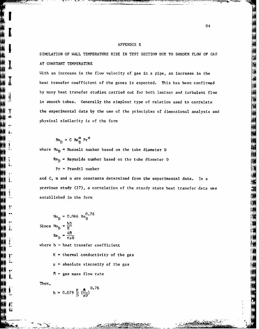
84

APPENDIX E

SIMULATION OF WALL TEMPERATURE RISE IN TEST SECTION DUE TO SUDDEN FLOW OF GAS[

AT CONSTANT TEMPERATURE

= With an increase in the flow velocity of gas in a pipe, an increase in the

heat transfer coefficient of the gases is expected. This has been confirmed

by many heat transfer studies carried out for both laminar and turbulent flow

; in smooth tubes. Generally the simplest type of relation used to correlate

the experimental data by the use of the principles of dimensional analysis and

physical similarity is of the form

- m rnNuD C Re D

where NuD = Nusselt number based on the tube diameter D

ReD = Reynolds number based on the tube diameter D

Pr = Prandtl number

and C, m and n are constants determined from the experimental data. In a

previous study (27), a correlation of the steady state heat transfer data ,as

established in the form

Nu = 0.066 Re0 .7 6

D D- hD

Since NuD

ReD = liDD -tjD

where h = heat transfer coefficient

K = thermal conductivity of the gas

u=absolute viscosity of the gas

= gas mass flow rate

Then,

0.76h = 0.079 (-)

D D)

ELI

85

IFor flow of gas at a constant temperature, the gas properties will remain

fairly constant and hence corresponding to the gas mass flow rate an

approximate alue for the heaL transfer coefficient can be obtained. Thus it

seemed feasible to determine the effect on the wall temperature due to a

sudden flow of gas at a constant temperature by using a stepwise function for

the heat transfer coefficient and neglecting flow acceleration.

A computer prograv using the finite difference approach was used to

E determine the gas side wall temrerature when subjected o a stepwise function

of the heat transfer coefficient of the gas. A transient energy balance can

be made on a node, m, on the surface of wall (See Figure 6.2) by setting the

sum of the energy conducted and convected into the node equal to the increase

in the internal energy of the node

(T _ TJ) (T 1i Tj )kA((m-l m +hAT T) CAAx m mAx g AT i 2 At

iJ Rearranging,A(Ax)2 2hJAx

T 2 N Tg + 2 T1 + T{ 2}]

m .x-,2 k 9hM-1 _ _ __k

• Thus the gas side wall temperature can be determined as a function of time

given the stepwise function for the heat transfer coefficient and the initial

temperature distribition in the wall. The simulation was carried out for

various engine speeds and the effect on the wall temperature determined up to

the desired crank angle in the engine cycle. The initial temperature

distribution in the wall required by the simulation program was calculated

from the actual experimental data.

186I APPENDIX F

GRAPHS OF MEASURED AND CALCULATED DATA

IThe graphs presented in this appendix depict the gas side walltemperature, Twall ' the exhaust gas temperature, Tgas and the exhaust gas mass

flow rate ,R as a function of the crank angle for different engine conditions

at each of the four positions in the test section. The gas temperature was

ensemble averaged over ten engine cylces while the wall temperatures curve

plotted was obtained from a single engine cycle for the same engine

condition.

MA-W

L-

87

0O 0m C) Cco

C) C0 ) C 0 CD ) CD C

m -0')t c C

th C)

Lo

ix -0 .0-

4-11

- 0

C) 0-

88

(.A14 WqL )Wk

co C0

LO 0o 0 0

cIc

CD-

C) CY

1 i 00 -

0to

I--

~C~) 0 r- ~ ~U)Cc )

U C~~~= C-)0 0 ~ O

EN- -~ I- i c -I

89

LflC C)J CD~

co ~ ~ (~ SOCM2 C Cm_ to m C 0 0

co an r-I LO m~ .c cm~ - e - n

ar_ _ _ _ _ __ _ _ _ _ _ 0

Lo I

S- -4

0 I 3

9 0

oc

to tn t o ou

LLLM.-

31si--

L LPMLOCh C) C C C C

(\Jcl co -.rC'j -

r CCD

I -4- N

I C)

C CCo

-~S- C:)

0 C)clfl

LOL

91 M

wqj

oo CD 0 0 0

1e_ I I I

CD C ) CD C CC) CIC ) CD C DCL I

I it /-, -au

I--

I~ -D

4-.C)I

C) m SI

C)/72 IcnL

Il

92

A (q/ wqL W C

Co C) C () ) tzr

r ~ 0 C)

SI PO

IC

12 CD 4"ra /o LO 4-I

(D 00-

M:o C C C C)

El (J)OPM

- --CD w

_ _ _ _c

In93

CD C) C>)

co 0o 0 0 o

0i

A LL

L HoLL

IL)4-i

TY I- C\

- I --.

oc

m 0 CD

0

1.0 00 ~ 0 k'.

I1 LPM-

UU

Li 94

I 22 J I / q lWc o U *O C j 000c n )

II i

Is L

i K!i

LL

7 1 c~)C)

-leU

I 04 4-A

4 11

SLLP14

CM

1 95

co 0CI

IC) C) C) C). C) C) C0C

cn LO C

r~co

i3-%

S- -Wh 4- M-1=~t CoI1

- 0~. c

I ~~- - - -

0 CDLL~

__ 1 96

0C) CJ 0C0

C~i C) ) C)

(j CD C- CD C- C) C

C)9- cn

-S

IIIf

C)~~ C)C

U.).

CT

97

co~~~ tqO wcu C) wD C) >

CDI C) DC CD CDC ~ ~ ~ d0 LO M0) C

I CD

LO D jo,

I C)

- I_

0

I C=)

LO CY

L ~L LeM*1(J.)

98

Aqu/ wqL W

00 0 0l C) C C)0%.0 co C 0 0

m(j a) O

Cl

I L /

V(

- 4 -

%--,I

L 1

0Jr

CD

CC

10 ? Ix. aDC)

00~l

0-) 1 e

99

(q/ wqL W

mi

C) ) D C C CD C- Cm- m -O p)C

U~ K - L

0l)

Ic~CD

cm1 CD

IIF-

0

UD LA0 -L nt LO

LLR

100

(l) Ci.

(YU -) ts t

M~ C)

hrj clIi / C0II-

Cl0

-- ------

C

L _ _

I-) C l

Ti eM

101

C(j S) 29

00 0 0 0)

CD, C CD C:) C) CD v

-C)i

br-LO .-

I coo

-I-

/ ~CD-

CD [AU ~ l :

0n :0 clj V0

Le~- - - -

102

( Aq/ wq~ L C

co Lr([') SPD C

CCi 01 (C)C)CeJcmJ CDJ -

C~j C0

I I Nj

C:I /c

M co

-~4/

CC)

iE~yy c:>K

1 01

0 -

C)J C\

Il l l

1A

103

SI,I APPENDIX G

COMPUTER PROGRAMS

C THE FOLLOWING PROGRAM USES CRANK ANGLE PULSES TO EXTERNALLYC TRIGGER THE DIGITISATION OF THE ANALOG SIGNALS WITH THE AIDC OF A REAL TIME SAMPLING (RTS) ROUTINE ON A PDP 11 MINI-C COMPUTER.

MAIN PROGRAMI DIMENSION IBUF (12000)I DATA K/li/

TYPE 5

TY PFORMAT(2X,-NAME OUTPUT DATA FILE-)CALL ASSIGN(li)UMW,-16NEW', )

C SET THE FLAGICMF=0

C SAMPLING DRIVEN BY S.T.#1C CALL RTS(IBUF,12000,,2400,,5,,0,ICMFIBEF)C WAIT FOR COMPLETION

CALL LWAIT(ICMF,0)_ TYPE 10

10 FORMAT(//,5X,-ICHAN1,2X,-ICHAN2",2X,IhAN3-,12X, "ICHAN4",2X, 'ICHAN5")DO 30 J=1,2400WRITE(1,20)IBUF(K),IBUF(K+1),IBUF(K+2),IBUF(K+3),IBUF(K+4)

20 FORMAT(5(I5))TYPE 25,IBUF(K),IBUF(K+1),IBUF(K+2),IBUF(K+3),IBUF(K+4)

25 FORMAT(5X,5(2X,I5))K=K+5

30 CONTINUECALL CLOSE(!)STOPENDI

C THE FOLLOWING PROGRAM SCANS THE DIGITISED DATA FORC ENGINE CYCLES,COMPILES THEM,DELETES THE DEFECTIVEC CYCLES AND THEN PROCESSES THEM INTO THEIR ACTUAL VALUES.C PROGRAM VALUE THEN USES A FINITE-DIFFERENCE METHODC TO DETERMINE THE INSTANTANEOUS HEAT FLUX AND HEATC TRANSFER COEFFICIENT FOR EACH INDIVIDUAL ENGINE CYCLEC AND THEN FINALLY ENSEMBLE AVERAGES THEM TO OBTAIN ONEC AVERAGED ENGINE CYCLE.

PROGRAM VALUEC (INPUT,OUTPUT,TAPE7,TAPE6) iDIMENSION IBUF3(53,241),IBUF4(241),IBUF5(241),SUM1(241)

-- -- A A

104

1,SUM2 (241) ,SUM4 (241) ,Q(241) ,H(241) ,X(21) ,Y(21) ,A(53,241)REAL K,IBUF3,IBUF4,IDUF5DATA X/2.0,2.1,2.2,2.3,2.4,2.5,2.6,2.7,2.8,2.9,3.0,3.11,3.2,3.3,3.4,3.5,3.6,3.7,3.8,3.9,4.0/DATA Y/520., 725.,932.,1105.,1235.,1350.,1445.,1540.1

C1635. ,1720. ,1805. ,1895. ,1995. ,2090. ,2180. ,2260. ,2340.:1 C,2430. ,2520. ,2610. ,2700./PRINT *,"N OF 'CYCLES TO AVG="READ *,MMPRINT *,IIFOR DELETING FIRST 120 PTS TYPE 1 ELSE 2"READ *JPRINT *,"GAS WALL TEMP (BIAS) ="READ *,TWALLCPRINT *,"WATER WALL TEMP="1READ *,TINITPRINT *,"RPM="t7 READ *,NNPRINT *,"SIF GAS WALL TEMP AMPLIFIED X5 TYPE 1 ELSE 2"

T READ *,IPPRINT *,IIF GAS TEMP AMPLIFIED X5 TYPE 1 ELSE 2"1READ *,IJKPRINT *,"ADDITIONAL GAS TEMP BIAS OVER 2V="READ *,ABPRINT *"AX~ ITERATIONS="

10 KP=5.

27IF (IP. EQ. 1) GO TO 10

GO TO 29

T 28 GF=5.29 DO 30 I=1r2130 X (1)=X (I) +AB31 DO 33 I=1,240

READ(7,32)IBUF3(53,I),IBUF4(I),IBUF5(I)32 FORMAT(1oX,3F5.0)

IF(I.LT.6)GO TO 33

IF(IBUF5(I).GT.3000.)GO TO 34I33 CONTINUE34 PRINT *,"'DO LOOP 13 COUNTER SUFF"

IF(JP.EQ.1)GO TO 36GO TO37

36 JP=JP+5GO TO 31

37 KK=O

A 1 -75 C--~- ~r~~-~TZ

105

Do 40 I=1,240RBAD(7,38)IBUF3(53,1) ,IBUF4(I) ,IBUF5(I)

38 FORI4AT(10X,3F5.0)I JJ=0IF(I.LT.10)GO TO 40IF(IBUF5(I).GT.3000.)GO TO 39GO TO 40

39 N=IGO TO 41

40 CONTINUE41 IF(N.EQ.120)GO TO 42

IF(N.GT.120)GO TO 37JJ=1

42 DO 45 I=1,240READ(7,43)IBUF3(53,I+120),IBUF4(I+120),IBUF5(II120)

43 FORMAT(10X,3F5.0)i-c(I.LT.10)GO TO 45IF(IBUFS(I+120).GT.3000.)GO TO 44GO TO 45

44 M=IGO TO 46

45 CONTINUE46 IF(M.GT.120)GO TO 42

IF(JJ.EQ.1)GO TO 37IB'(M.EQ.120)GO TO 47GO TO 37

47 PRINT *,t240 PTS CHECK SUCESSFUL"C

Do 52 I=1,240IBUF3(53,I)=(IBUF3(53,I)-2048.)*0.0025IBUF4 (I)=(IBUF4 (I) -2048.) *0.0025IBUF3(53,I)=TWALLC+(IBUF3(53,I)*1000.*3./(0.0227*2000*28.

1*GF))IBUF4 (I) =IBUF4 (I) *4./APIF(IBtJF4(I).GT.X(21))GO TO 74IF(IBUF4(I).GE.X(1))GO TO 49

IF(IBUF4(I).GT.0.)GO TO 52IF(I.EQ.1)GO TO 80IBUF4 (I) =IBUF4 (I-1)GO TO 52

49 DO 51 J=1,21IF(IBUF4(I).EQ.X(J))GO TO 50GO TO 51

50 IBUF4 (I) =Y (J)GO TO 52

51 CONTINUEMl+ (IBUF4 (I) -X (1))/0. 1

52 CONTINUEI ~IBUF3 (53, 241) =IBUF3 (53, 240)

106

IBUF4 (241) =IBUF4 (240)C

DO 53 J=1,241I53 TAVG=TAVG+IBUF3(53,J)TAVG=TAVG/2 41.DELTIM=1./(2. *NN)DELX=. 156/52COEFF=ALPHA*DELTIM/(DL*2

DO 54 I=1,52I ~IBUF3 (1,1) =TINIT-I(TAVG-TINIT) *ZZ/.15654 ZZ=ZZ+0.00355 IBUF3(1,1)=TINIT

KK=KK+1,JK=ODO 57 J=1,239I IBUF3 (1,J+1) =TINITDO 56 I=2,52

- I C+IBUF3(I,J)*(1-2*COEFF)I IF(KK.EQ.1)GO TO 25

25 AJ1)=BUF3(I,J+1)-AIJ1)IU3IJ1)G.01J~

56 CONTINUE57 CONTINUEr

IF(KK.EQ.1)GO TO 26IF(KK.EQ.KMAX)GO TO 75IF(JK.EQ.1)GO TO 26GO TO 59

26 DO 58 I=1,53ii ~IBUF3 (I, 1) =IBUF3 (I, 240)

58 CONTINUEGO TO 55

59 QAVG=0.DO 60 J=1,240Q(J) =(IBUF3 (53,J) -IBUF3 (52,J) )*K/DELx+(IBUF3 (53,J+1)

C-IBU'3 (53,J) )*K/(DELX*2*COEFF)QAVG=QAVG+Q (J)[

60 CONTINUEQAVG=QAVG/240.

IF(KP.GT.0)GO TO 63Lai DO 62 I=1,240

SUM2(I)=0.I SUM4 (I) =0.62 CONTINUE63 KP=KP+1I DO 64 I=1,240

------- --

107

i ~ ~SUM1(I) =SUM! (I) +Q (I)

SUM2 (I) =SUM2 (I) +H (I)SUM4 (I) =SUM4 (I) +IBUF4 (I)

64 CONTINUEIF(KP.EQ.MM)GO TO 65

GO TO 3765 PRINT *,"NO OF CYCLES TO AVG=',KP

DO 68 I=1,240SUM1(I)=SUM1(I)/KPSUM2 (I) =SUM2 (I)/KPSUM4 (I) =SUM4 (I)/KP

68 CONTINUEC DO 100 I=1,53C WRITE(6,101)IBUF3(I,240)C101 FORMAT(10X,F15.10)CI00 CONTINUE

DD=1.E9DO 66 I=1,240IF(IBUF3(53,I).LT.DD)DD=IBUF3(53,I)

66 CONTINUEDO 67 I=1,240IBUF3 (53,I) =IBUF3 (53,I) -DD

67 CONTINUEC WRITE(6,69)C69 FORMAT(//,9X,"Q(J)",8X,"T(53,J)" 9X,"T(52,J)",7X,C C"TGAS(J) ",1OX,"H(J) ",/)

DO 73 J=i,240WRITE(6,71)SUM1(J),IBUF3(53,J),IBUF3(52,J),SUM4(J),SUM2(J)71 FORMAT (El5.6,4F15.6)

73 CONTINUEGO TO 76

74 PRINT *,"GAS TEMP INTERVAL INSUFF ON HIGH SIDE"GO TO 76I75 PRINT *?"CONVERGENCE FAILED"PRINT *,"INCREASE THE MAX NO OF ITERATIONS"GO TO 76

80 PRINT *,"FIRST VALUE OF GAS TEMP NEGATIVE"76 STOP

END

T C THE FOLLOWING PROGRAM USES CORRECTED INSTANTANEOUSC UPSTREAM AND DOWNSTREAM PRESSURES TO COMPUTE THE

, C INSTANTANEOUS EXHAUST GASS MASS FLOW RATE.

PROGRAM PCORR (FINAL1, TAPE5=FINAL1, TEMPI, TAPE6=TEMP1, INPUT,

1OUTPUT)DIMENSION SUM1(241) ,SUM2(241) ,SUM4 (241) ,MEXH(241)REAL MEXH,MTOT

-AM

108

DATA CC/-1.EIO/,D1)/1.El0/,EIE/-1.ElO/,FF/1 iG,

GC=32. 174GAIMA=1.3RGAS=1544./28.59B=0.55CV=0.72P1=3. 141599D=1. 125/12.MTOT=0.PRINT *,"PRESS2 CORRECTION TERM:LOWER BY ? PSI"

RED*, PCORR2

PRINT *j"SHIFT PRESS2 DOWN(PHASE-LAG) :HOW MANY PTS?"READ *,IPDO 25 I=1,240READ(5,10-)SUM1(I) ,SUM2(I) ,SUM4(I)

10 FORMAT(2(lX,F14.6) ,16X,F14.6)

SUM2 (I-IP) =SUM2 (I)_ I GO TO 25

20 SUM2(240-IP+I)=SUM2(I)25 CONTINUE

DO 70 I=1,240II30 KL1lIF(SUM1(I).GE.SUM2(I))GO TO 40I A=SUM1 (I)SUMi (I) =SUM2 (I)SUM2 (I) =A

40 KL=-l40 Fl=SQRT(2.*GC*GAMMA*((SUM1(I)*144.)**2)/((GAMA-1)

1*RGAS*(459.67+SUM4(I))))F2=SQRT( ( ((SUM2(I)/SUM1(I) )**(2 /GAMMA) )-( (SUM2(I)

2/SUM1(I))**(2./GAMMA)))))MEXH(I) =( (CV*PI* (D**2) *(B**2) )/4.) *Fl*F2*KL*3600.IF(KL.EQ.1)GO TO 50BB=SUM1 (1)SUMi (I) =SUM2 (I)

ft SUbM2 (I)=BB3 50 IF(SUM1(I) .GT.CC)CC=SUM1(I)

IF(SUM1(I) .LT.DD)DD=SUM1(I)IF (SUM2 (I) . GT. EE) EE=SUM2 (I)IF(SUM2 (I).LT.FF) FF=SUM2 (I)IF(MEXH(I) .GT.GG)GG=MEXH(I)IF (MEXH (I) .LT. HH) HH=MEXH (I)WRITE(6,60)SUM1(I) ,SUM2(I) ,MEXH(I)I 60 FORMAT(2(1X,FJ.4.6) ,1X,E15.7)MTOT=MTOT+MEXH (I)

70 CONTINUEMTQT=MTOT/140.

LA_ -m

109

PRINT *, "MTOT" l,MTOT, "LBS/HR"'PRINT *,flPRESS1 MAX=",CCPRINT *, "PRESS1 MIN=",DDPRINT *,I"PpRE55 MAX=",EEPRINT *,IIPRESS2 MIN",FFPRINT *,HMEXH MAX=",GGIPRINT *,'MEXH MIN=",HHSTOP

END

C THE FOLLOWING PROGRAM USES THE FINITE-DIFFERENCE METHODc TO OBTAIN THE TEMPERATURE DISTRIBUTION IN A FLAT PLATEI

C WITH ONE SURFACE TEMPERATURE A KNOWN PERIODiC FUNCTIONC OF TIME.

PROGRAM FDIFF (TEMP, TAPE6=TEMP, INPUT, OUTPUT)DIMENSION T(53,241) ,Q(240) ,A(53,241)REAL KTINIT=2.PRINT *,"MAX ITERATIONS="READi~ *,KM4JXKK=OPI=3.141597TA=2.THETA=0.1DO 10 J=1,241F= (J-1) /2400.I: T(53,J) =TA*COS(2. *PI*F/THETA)

10 CONTINUEALPHA=0. 0055K=0.00023DELTIM0. 1/240PRINT * ,"DELTIM"l, DELTIMDELX=. 156/52COEFF=ALPHA*DELTIM/ (DELX**2)DO 20 I=1,52T(I,1) =TINIT

20 CONTINUE21 T(1,1)=TINIT

JK=OLKK=KK+1DO 40 J=1,239T(1,J+1) =TINIT

ijDO TO 29,5T(I,J+1) =COEFF*(T(I+1,J)+T(I-1,J) )+T(I,J) * (1A2*COEFF)

29 A(I,J+1)=T(I,J+1)

110

30 CONTINUE40 CONTINUE

IF(KK.EQ.1)GO TO 71I IF(KK.EQ.KMAX)GO TO 90IF(JK.EQ.1)GO TO 71QTOT=0 .0I DO 50 J=1,240Q(J)=(T(53,J)-T(52,J) )*K/DELX+(T(53,J+1).T(53,J))1*K/ (DELX*2. *COEFF)QTOT=QTOT+Q (J)

50 CONTINUEQTOT=QTOT/240.1C WRITE(6,51)QTOT

C51 FORMAT(//,9X,"QTOT=",5X,E15.6)C WRITE(6,60)C60 FOR.NAT(///,9X,"Q(J),8X,"T(53,J)",9X,"T(52,J)")

AA=0.

DD=99999999.

DO 70 J=1,240IF(Q(J) .GT.AA)AA=Q(J)IF(Q(J) .LT.BB)BB=Q(J)IF(T(53,J) .GT.CC)CC=T(53,J)IF(T(53,J) .LT.DD)DD=T(53,J)WRITE(6,65)Q(J) ,T(53,J) ,T(52,J)

65 FORMAT(El5.6,2FI5.6)70 CONTINUE

PRINT *, "QMAX=" ,AA, "QMIN=" ,BBPRINT ~,"T(53,J)MAX=",CC,"T(53,J)MIN=",DDGO TO 80

C71 PRINT *, t 'KKI'l,KK71 DO 75 I=1,53

T (1,1) =T (1,240)75 CONTINUE

GO TO 2180 PRINT *?"CONVERGENCE SUCCESSFUL"

PRINT *,"NO OF CYCLES FOR CONVERGENCE=",KKGO TO 100

90 PRINT *,"'CONVERGENCE FAILED"PRINT *"INCREASE THE MAX NO OF ITERATIONS"3

100 STOPEND

C THE FOLLOWING PROGRAM USES A FOURIER-SERIES EXPANSIONC METHOD TO OBTAIN THE TEMPERATURE DISTRIBUTION IN AC FLAT PLATE WITH ONE SURFACE TEMPERATURE A KNOWN PERIODICC FUNCTION OF TIME.

4Ilid

PROGRAM SERIES (INPUT,C, TAPE6=CHECK ,OUTPUT)DIMENSION Q(50) ,QDOT(241) ,TS(241)REAL L,KPI=3.141597L.156TM=2.OTHETA0. 1K=0. 00023A=0. 0055B=SQRT( (PI*(L**2) )/(A*THETA))PRINT ~,"MAX NO OF TERMS FOR SUMMATION"READ *,LP

C WRITE(6,25)JIC25 FORMAT(8X,-QDOT(M) ",10X,-SURFACE TEMP',//)

DO 300 M=1,241F= (M-1) /2400.G=2.*PI*F/THETATS (M) =TM*COS (2. *PI*F/THETA)

QD=Q (1)DO 200 I=1,LPX= IJJ=X/2IF(I.EQ. (2*JJ))D=0.IF(I.NE. (2*JJ))D=1.Q(I+1)=( (-1) **(2*I) )*B*EXP(-B* (I-ID) )*(SIN(G..B*(I+D))1-COS (G-B* (I+D)) ) LQD=QD+Q (1+1)IF(ABS((Q(I+1)-Q(I))/Q(I+1)).LT..001)GO TO 201

200 CONTINUEPRINT *,"CONVERGENCE FAILED"GO TO 101

201 PRINT *,"NO OF TERMS SUMMED=1fXQDOT (M)=-K*TM*QDWqRITE(6,75)QDOT(M) ,TS(M)

75 FORMAT(2X,E15.6,2X,F1S.6)300 CONTINUE

WRITE(6,50)50 FORMAT(//,5X,"Q(J) ",//)

DO 100 I=1,11IL WRITE (6, 150) Q ( I)

150 FORMAT(2X,E15.6)100 CONTINUE101 STOP

END

C THIS PROGRAM SIMULATES THE WALL TEMPERATURE RISE IN THEC TEST SECTION DUE TO FLOW OF GAS AT A CONSTANT TEMPERATUREIC AT VARIOUS ENGINE SPEEDS WITH THE USE OF AN INITIAL

112

C TEMPERATURE DISTRIBUTION IN THE WALL CALCULATED FROM THEC EXPERIMENTAL DATA AND A STEPWISE FUNCTION FOR THE HEATC TRANSFER COEFFICIENT.

PROGRAM PULSE (INPUT, OUTPUT, TAPE8 ,TAPE9)DIMENSION T(53,241) ,H(241) ,TGAS(241) ,BIOTNO(241) ,TSWING(241)1, THETA (241)REAL K

READ *,TINITPRINT * ,"ARP ALL EPRTR=RINT *,"PM&

PRINT *,"VALUE OF GAS TEMPERATURE"READ1 *,TGPRINT *,"STEP INPUT VALUE OF H"tREAD *,flGPRINT *,"TEMPERATURE RISE TILL WHAT CRANK ANGLE"

READ *,ICAIDO 10 J=1,241H(J) =HG/ (144. *3600.)TGAS (J)=TG

10 CONTINUEDO 12 I=1,53

I READ(8,11)T(I,1)11 FORMAT(1OX,F15.10)12 CONTINUE j

ALPHA=0.0055K=0.00023DELTIM=1./ (2. *NN)DELX=0.156/52COEFF=ALPHA*DELTIM/ (DELX* *2)[THETA(1) =0.T(1,1) =TINITTSWING (1) =0.DO 14 J=1,239T(1,J+1) =TINITBIOTNO (J) =H (J) *DELX/KDO 13 I=2,52T(I,J+1)=C0EFF*(T(I+1,J)+T(I-1,J) )+T(I,J) *(1.-2.*COEFF)

13 CONTINUET(53,J+1)=COEFF*(2.*T(52,J)+2.*BIOTNO(J)*TGAS(J)+T(53,J)

C*((1./COEFF)-2.*BIOTNO(J)-2.))TSWING(J+1)=T(53,J+1)-T(53,1)THETA (J+1) =3*J

14 CONTINUEKJ=ICA/3+1DO 16 J=1,KJWRITE(9,15)THETA(J) ,TSWING(J)

15 FORMAT(5X,F5.1,10X,F1O 5)

L 16 CONTINUEt

113

WRITE(9,17)TINIT17 FORMAT(//,5X,"'TINIT=",FlO.4)

WRITE(9,18) T(53,1)18 FORMAT(/,5X,"T(53>,l)="F10.4)

STOPEND

C THE FOLLOWING IS A TYPICAL PLOTTING ROUTINE USED TOC PLOT THE INSTANTANEOUS HEAT FLUX. HEAT TRANSFER COEFF.,C SURFACE WALL TEMPERATURE SWING AND THE EXHAUST GAS I

C TEMPERATURE AS A FUNCTION OF THE CRANK ANGLE.

PROGRAM PLCT5 (INPUT, OUTPUT, TAPEl, TAPE2, TAPE3 ,TAPE4 ,TAPE5O=1OUTPUT)VDIMENSION 241q) ,Y1(241) ,Y2(241) ,Y3(241) ,Y4(241)C,A1(241) ,A2 (241) ,A3 (241) ,A4(241)PRINT *,-TYPE 1 FOR Q,2 FOR TWALL,3 FOR TGAS,4 FOR H-READ *'JJPRINT *, "INPUT YMIN,-.MAX,YTICK,ND"READ *,YMIN,YMAjX,YTICi(,NDCALL PLOTS(O.,0.,50)CALL BOX(0.:720.,90.,1l,YMIN ,YMAX ,YTICK,ND)CALL XLABEL("CRANK ANGLE!Z-,0)IF (JJ. EQ. 1) GO TO 13IF (JJ. EQ. 2) GO TO 16IF (JJ.EQ.3)GO TO 19DO 12 I=1,240READ (1, 11) Yl(I)

11 FORMAT-(60X,F15.6)READ (2, 25) Y2(I)

25 FORM.AT(60X,F15.6)READ (3, 26) Y3(I)

26 FORMAT(60X,F15.6)READ (4, 27) Y4 (I)

27 FORMAT(60X,F15.6)12 CONTINUE

CALL YLABEL("H (BTU/SQ.FTf/HR/DEG.F) !Z"0)

13 DO 15 I=1,240

28 FORZMAT(E15.6)READ (2,28) Y2(I)

28 FORMAT(E1L5.6)READ (3,320) Y3(I)

30 FORMAT(E15.6)

15 CONTINUE ra

114

= CALL YLABEL("Q/A (BTU/SQ. IN/SEC) !Z",0)GO TO 5O

16 X(1)=0IDO 70 I=1,240X(I+1) =1*3

70 CONTINUEDO 18 I=1,240RED(,3)Y I

31 FORMAT(15X,Fl5.6)READ (2, 32) Y2(I)

32 FORMAT(15X,F15.6)LSREAD (3, 33) Y3 (I)I

33 FORMAT(15X,F15.6)-IREAD (4, 34) Y4(I)34 FORMAT(15X,F15.6)18 CONTINUEI3: Y1 (241) =Y1 (240)

Y2 (21) =Y (240

Y3 (241) =Y3 (240)Y4 (241) =Y4 (240)

= CALL YLABEL("WALL TEMP SWING(DEG)!Z",0)GO TO 22

19 X(1)=0DO 80 I=1,240X(I+1) =1*3

780 CONTINUEDO 21 I=1,240

20 FORMAT(45X,F15.6)READ (2, 35) Y2(I)

35 FORMAT(45X,F15.6)READ (3, 36) Y3(I)

36 FORMAT(45X,Fl5.6)READ(4,37)Y4 (4

37 FORMAT(45X,F15.6)21 CONTINUE

Y1 (241)=Y1 (240)Y2 (241) =Y2 (240)Y3 (241) =Y3 (240)Y4 (241) =Y4 (240)I CALL YLABEL(-GAS TEMP (DEG.F)!Z",0)GO TO 22

50 DO 60 I=1,240Al (I)=Y1 (I)A2(I)=Y2(I)A3(I)=Y3(I)A4 (I) =Y4 (I):3:60 CONTINUEX(1)=0DO 40 I=2,240X (I)=(1-1) *3-. j5

Fir: ______ -~-- =--- __

115

Yl1(I)=(Al1(I-1) +A 1) )/2._ Y2(I)=(A2(I-1)+A2(I))/2.

Y3 (I) =(A3 (I-1) +A3 (I) ) /2.Y4 (I) =(A4 (I-1) +A4(1)) )/2.

40 CONTINUEX(241) =717Yl (241) =Al (240)Y2 (241) =A2 (240)

Y3 (241)=A3 (240)Y4 (241) =A4 (240)

22 CALL LEGEND(O.0,0.O,0.0,0.0)CALL LPLOT(X,Y1,241,1,0)CALL LPLOT(X,Y2,241,1,0)CALL LPLOT(X,Y3,241,1,0)CALL LPLOT(X,Y4,241,1,0)CALL PLOT(0.,0.,999)PRINT *,tlTYPE,TA.PE50 TO PLOT-STOPEND

13

no-

r

®R