identification of low order equivalent system models …mln/ltrs-pdfs/nasa-2000-tm210117.pdf ·...
TRANSCRIPT

August 2000
NASA/TM-2000-210117
Identification of Low Order EquivalentSystem Models From Flight Test Data
Eugene A. MorelliLangley Research Center, Hampton, Virginia

The NASA STI Program Office ... in Profile
Since its founding, NASA has been dedicatedto the advancement of aeronautics and spacescience. The NASA Scientific and TechnicalInformation (STI) Program Office plays a keypart in helping NASA maintain this importantrole.
The NASA STI Program Office is operated byLangley Research Center, the lead center forNASAÕs scientific and technical information.The NASA STI Program Office providesaccess to the NASA STI Database, the largestcollection of aeronautical and space scienceSTI in the world. The Program Office is alsoNASAÕs institutional mechanism fordisseminating the results of its research anddevelopment activities. These results arepublished by NASA in the NASA STI ReportSeries, which includes the following reporttypes:
· TECHNICAL PUBLICATION. Reports
of completed research or a majorsignificant phase of research thatpresent the results of NASA programsand include extensive data or theoreticalanalysis. Includes compilations ofsignificant scientific and technical dataand information deemed to be ofcontinuing reference value. NASAcounterpart of peer-reviewed formalprofessional papers, but having lessstringent limitations on manuscriptlength and extent of graphicpresentations.
· TECHNICAL MEMORANDUM.
Scientific and technical findings that arepreliminary or of specialized interest,e.g., quick release reports, workingpapers, and bibliographies that containminimal annotation. Does not containextensive analysis.
· CONTRACTOR REPORT. Scientific and
technical findings by NASA-sponsoredcontractors and grantees.
· CONFERENCE PUBLICATION.Collected papers from scientific andtechnical conferences, symposia,seminars, or other meetings sponsoredor co-sponsored by NASA.
· SPECIAL PUBLICATION. Scientific,
technical, or historical information fromNASA programs, projects, and missions,often concerned with subjects havingsubstantial public interest.
· TECHNICAL TRANSLATION. English-
language translations of foreignscientific and technical materialpertinent to NASAÕs mission.
Specialized services that complement theSTI Program OfficeÕs diverse offeringsinclude creating custom thesauri, buildingcustomized databases, organizing andpublishing research results ... evenproviding videos.
For more information about the NASA STIProgram Office, see the following:
· Access the NASA STI Program HomePage at http://www.sti.nasa.gov
· E-mail your question via the Internet to
[email protected] · Fax your question to the NASA STI
Help Desk at (301) 621-0134 · Phone the NASA STI Help Desk at
(301) 621-0390 · Write to:
NASA STI Help Desk NASA Center for AeroSpace Information 7121 Standard Drive Hanover, MD 21076-1320

National Aeronautics andSpace Administration
Langley Research CenterHampton, Virginia 23681-2199
August 2000
NASA/TM-2000-210117
Identification of Low Order EquivalentSystem Models From Flight Test Data
Eugene A. MorelliLangley Research Center, Hampton, Virginia

Available from:
NASA Center for AeroSpace Information (CASI) National Technical Information Service (NTIS)7121 Standard Drive 5285 Port Royal RoadHanover, MD 21076-1320 Springfield, VA 22161-2171(301) 621-0390 (703) 605-6000

i
Table of Contents
ABSTRACT ...................................................................................................................................ii
NOMENCLATURE .....................................................................................................................iii
SUPERSCRIPTS...............................................................................................................................v
SUBSCRIPTS ..................................................................................................................................v
I. INTRODUCTION ....................................................................................................................1
II. THEORY .................................................................................................................................3
MODEL FORMS .............................................................................................................................3
PARAMETER ESTIMATION METHODS............................................................................................8
Output Error in the Frequency Domain..................................................................................8
Equation Error in the Frequency Domain ............................................................................11
PARAMETER CORRELATION ANALYSIS.......................................................................................15
Output Error..........................................................................................................................15
Equation Error ......................................................................................................................21
LOES MODELING ISSUES...........................................................................................................22
III. SIMULATION EXAMPLES ..............................................................................................29
IV. FLIGHT TEST EXAMPLES .............................................................................................39
V. SUMMARY............................................................................................................................43
VI. REFERENCES.....................................................................................................................44
VII. TABLES ..............................................................................................................................47
VIII. FIGURES...........................................................................................................................54

ii
Abstract
Identification of low order equivalent system dynamic models from flight test data was
studied. Inputs were pilot control deflections, and outputs were aircraft responses, so the models
characterized the total aircraft response including bare airframe and flight control system.
Theoretical investigations were conducted and related to results found in the literature. Low
order equivalent system modeling techniques using output error and equation error parameter
estimation in the frequency domain were developed and validated on simulation data. It was
found that some common difficulties encountered in identifying closed loop low order equivalent
system models from flight test data could be overcome using the developed techniques.
Implications for data requirements and experiment design were discussed. The developed
methods were demonstrated using realistic simulation cases, then applied to closed loop flight
test data from the NASA F-18 High Alpha Research Vehicle.

iii
Nomenclature
az body axis vertical acceleration, g
c mean aerodynamic chord, ft
c.g. center of gravity
C parameter covariance matrix
E ¼; @ expected value
e equation error, or base of natural logarithm
FQ flying qualities
g gravitational acceleration = 32.174 ft/sec2
HARV High Alpha Research Vehicle
j imaginary number = −1
J cost function
K&θ gain for short period ~ ~q eη transfer function
L aerodynamic lift force, lbf
L, M, N aerodynamic roll, pitch, and yaw moments, ft-lbf
LOES Low Order Equivalent System
m number of discrete frequencies
np number of elements in parameter vector θ
N number of data points in the time domain
p, q, r roll, pitch, and yaw rates, rad/sec
P power spectral density
q dynamic pressure, lbf/ft2
Re real part of a complex number
s Laplace transform variable
See equation error covariance matrix
Sνν output error covariance matrix

iv
t time, sec
T data record length, sec
TR roll mode time constant
TS spiral mode time constant
1 Tθ 2numerator zero parameter for short period ~ ~q eη transfer function
v output error
V airspeed, ft/sec
w weight, lbf
xcg longitudinal center of gravity position, in
y model output
Y aerodynamic side force, lbf
z measured output
α angle of attack, rad
β sideslip angle, rad
∆ t sampling interval, sec
φ roll angle, rad
ϕ Bode plot phase angle, deg
ηa lateral stick deflection, in
ηe longitudinal stick deflection, in
ηr rudder pedal force, lbf
ν i1 6 noise vector at time i t−11 6∆θ parameter vector
Θ pitch angle, rad
σ 2 variance
τ time delay, sec
τ e longitudinal stick equivalent time delay, sec

v
τ a lateral stick equivalent time delay, sec
τ r rudder pedal equivalent time delay, sec
ω frequency, rad/sec
ω DR dutch roll natural frequency, rad/sec
ω sp short period natural frequency, rad/sec
ζ DR dutch roll damping ratio
ζ sp short period damping ratio
absolute value or modulus of a complex number
SUPERSCRIPTS
T transpose
† complex conjugate transpose
$ estimate
~ Laplace or Fourier transform
& time derivative
–1 matrix inverse
SUBSCRIPTS
avg average
E measured value from experiment
EE equation error
hos high order system
LOES low order equivalent system
LS least squares
OE output error
o nominal or trim value

1
I. Introduction
Many aircraft employ automatic flight control systems that include significant dynamics
attributable to the control law implementation, artificial feel systems, sensors, filters, and
actuators. The complexity of these control systems results from the desire for improved
performance and control over expanded flight envelopes, and from the ability to implement
lengthy calculations onboard the airplane in real time with small and fast flight control
computers.
Current flying qualities criteria and military specifications are based primarily on data from
unaugmented aircraft with classical dynamic responses. For linearized longitudinal dynamics,
the classical dynamic response is comprised of two damped oscillatory modes called the phugoid
(long period) mode and the short period mode. To apply the large body of information acquired
for unaugmented airplanes to airplanes whose dynamics are no longer classical because of
additional dynamics from the control system, the concept of a Low Order Equivalent System
(LOES) model was introduced1-3. The LOES model has the same form as the model for an open
loop unaugmented airplane with classical dynamic modes, except the inputs are pilot controls
with equivalent time delays, instead of control surface deflections. The equivalent time delay
was introduced to account for time delay resulting from the digital control system
implementation (e.g., sampling delay), and the phase lag at high frequency from control system
dynamics and various nonlinearities, such as control surface rate limiting.
The LOES model characterizes the linearized dynamic closed loop response of the airframe
and control system as it appears to the pilot. If the closed loop response of an augmented
airplane to pilot inputs can be accurately characterized using a LOES model, then specifications
for classical unaugmented aircraft parameters found in the current Military Specification for
Flying Qualities of Piloted Airplanes1 (hereafter called the Mil-Spec) can be applied directly to
the estimated parameters from a LOES model. The Mil-Spec quantifies the relationship between
parameter values in a low order dynamic model and pilot opinion as measured by flying qualities
levels1, which are based on pilot Cooper-Harper ratings4.
Many flight test research programs5-14 have demonstrated that the LOES concept can be
used to correlate pilot flying qualities levels with augmented aircraft dynamic response that is in

2
reality high order and nonlinear. LOES models of the aircraft dynamic response are fit over the
frequency band corresponding to typical pilot inputs, 0.1 – 10 rad/sec. Parameters from LOES
models can then be used with flying qualities specifications for classical low order model
parameters in the Mil-Spec to quantify and analyze flying qualities. The Mil-Spec also
documents the strong effect of time delay on Cooper-Harper ratings and includes specifications
relating flying qualities levels and time delay. Time delay is an important parameter, and is
estimated as part of the closed loop LOES model.
LOES models identified from flight test data are also useful for validating linear control law
designs, since the LOES model represents the achieved linearized closed loop dynamics of the
aircraft. LOES models can also be used for rudimentary simulation in the limited flight envelope
where the model is valid.
This work focused on identifying accurate low order equivalent system models for the
closed loop dynamics of augmented aircraft, based on measured flight test data. The methods
can be applied to identify LOES models using data from typical flying qualities evaluation
maneuvers such as tracking or landing tasks, and do not require specific system identification
maneuvers like frequency sweeps. A quantitative model of the closed loop aircraft response can
be identified using data from the same maneuver the pilot used to rate the flying qualities. Such
information is useful for flying qualities research and aircraft development. The techniques
described in this work address practical LOES modeling problems such as identifiability of
model parameters, limited data, frequency resolution, and variable model fidelity requirements
over the pilot input frequency range.
The next section includes theory and related investigations. Next, simulation examples
were used to demonstrate proposed approaches for accurate LOES modeling from measured
data. Finally, the modeling techniques were applied to data from flight test maneuvers of the
NASA F-18 High Alpha Research Vehicle (HARV).

3
II. Theory
MODEL FORMS
The model structure for LOES modeling is fixed a priori to correspond to classical linear
aircraft dynamic response with an input time delay. For the short period longitudinal dynamic
mode, the closed loop pitch rate response to longitudinal stick deflection is modeled in transfer
function form as1
~~
&q K s T e
s se
s
sp sp sp
e
η ζ ω ωθ θ
τ=
+
+ +
−1
2
2
2 2
3 83 8
(1)
The equivalent input time delay τe is included to account for additional phase lag from high
order control system dynamics, nonlinearities, and sampling delay. The current Mil-Spec1
correlates pilot opinion (via flying qualities levels) with ranges of values for all model
parameters in Eq. (1) except K&θ . If a LOES model can be identified that approximates the
closed-loop dynamic response over the bandwidth of the pilot, then the resulting estimated
parameters can be used in conjunction with the Mil-Spec to quantify flying qualities.
The problem addressed in this work is accurate estimation of the model parameters in
Eq. (1) using measured input-output flight test data. The idea is to match the measured outputs
or output time derivatives with the corresponding quantities from the model by adjusting the
model parameters to minimize a measure of fit error, usually the sum of the squared deviations
between model quantity and measured quantity. Several methods exist for estimating model
parameters based on measured data, both in the time domain15,16 and the frequency domain17-19.
One problem with the model parameterization in Eq. (1) is that the role of the gain
~ ~q seη with = 01 6 is not isolated to a single parameter, since the gain is K Tsp&θ θω 22
. Movement
of K Tsp&
, ,θ θω or 2
can account for changes in the gain when a parameter estimation algorithm
adjusts the free parameters to match measured data. In such cases, the parameters are said to be

4
correlated. Parameters Tθ2 and ω sp have other roles as well. Parameter Tθ2
is the negative
inverse of the numerator root, and ω sp is the natural frequency for the denominator quadratic
factor. These roles only become apparent at frequencies near or above 12
Tθ or ω sp . If most of
the measured data resides at low frequencies relative to 1 Tθ 2 and ω sp , the parameters
K Tsp&
, ,θ θω and 2
will be highly correlated, and the estimates of these parameters will be
indeterminate. The parameter estimation algorithm, given only low frequency data, cannot
determine which parameter to move to account for the gain, since movement of K Tsp&
, ,θ θω or 2
could be used to achieve a given gain.
Some improvement in the parameter correlation situation can be achieved by
re-parameterizing the model in Eq. (1) as
~~q b s b e
s a s ae
s
η
τ=
+
+ +
−1 0
21 0
1 63 8
(2)
or
~~q b s b e
a s a se
s
η
τ=
+
+ +
−1 0
22
1 1
1 63 8
(3)
The gain involves fewer parameters in Eqs. (2) and (3), which mitigates parameter correlations at
low frequency. The relationship among the parameters in Eqs (1)-(3) can be determined by
straightforward comparison. For example, the parameters in Eqs. (1) and (2) are related by:
b K b K T
a a
e
sp sp sp
1 0
1 02
2
2
= = =
= =
& &θ θ θ τ τ
ζ ω ω(4)

5
or
K b T b b
a a a
e
sp sp
&θ θ τ τ
ζ ω
= = =
= =
1 1 0
1 0 0
2
23 8(5)
Other model parameterizations are possible, such as
~~q b s b e
s se
s
sp sp spη ζ ω ω
τ=
+
+ +
−1 0
2 22
1 63 8
(6)
and
~~q
KT s e
ss
e
s
sp
sp
sp
η
ωζ
ω
θτ
=+
+ +���
���
−2
1
21
2
2
3 8
(7)
The LOES model can also be formulated as a state space model. Using the short period
approximation from classical airplane dynamics20, with the understanding that the stability and
control derivatives include the effects of bare airframe plus control system, the LOES model can
be written in state space form:
1 0
1
1
−�!
"$#�!
"$# =
− −�!
"$#�!
"$# +
−�!
"$#
−M q
L L
M M q
L
Mt
q
qe
e
e&
&
&α
α
α
η
η
α αη τ1 6 (8)
Assuming Lq ≈ 0 for low angles of attack, and assuming Leη ≈ 0 , which is typical,
1 0
1
1 0
−�!
"$#�!
"$# =
−�!
"$#�!
"$# +
�!
"$#
−M q
L
M M q Mt
qe
e&
&
&α
α
α η
α αη τ1 6 (9)
6
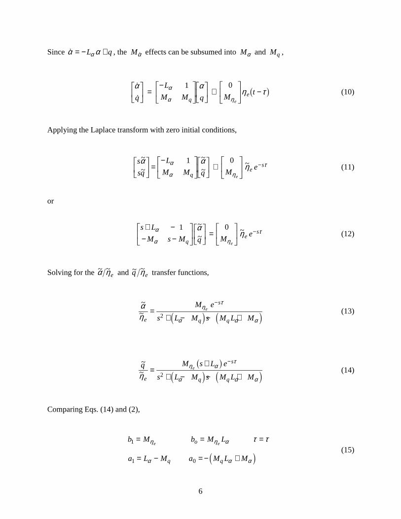
Since &α αα= − +L q , the M &α effects can be subsumed into Mα and Mq ,
&
&
α αη τα
α ηq
L
M M q Mt
qe
e
�!
"$# =
−�!
"$#�!
"$# +
�!
"$#
−1 0 1 6 (10)
Applying the Laplace transform with zero initial conditions,
s
sq
L
M M q Me
qe
s
e
~
~
~
~~α αηα
α ητ�
! "$# =
−�!
"$#�!
"$# +
�!
"$#
−1 0
(11)
or
s L
M s M q Me
qe
s
e
+ −− −
�!
"$#�!
"$# =
�!
"$#
−α
α ητα
η1 0~
~~ (12)
Solving for the ~ ~α ηe and ~ ~q eη transfer functions,
~
~αη
ητ
α α αe
s
q q
M e
s L M s M L Me=
+ − − +
−
2 3 8 3 8 (13)
~~q M s L e
s L M s M L Me
s
q q
e
ηη α
τ
α α α=
+
+ − − +
−1 63 8 3 82
(14)
Comparing Eqs. (14) and (2),
b M b M L
a L M a M L M
e eo
q q
1
1 0
= = =
= − = − +
η η α
α α α
τ τ
3 8(15)

7
or
M b L b b
Mb a b
bM
b
b
b a b
ba
e
q
η α
α
τ τ= = =
= − = − −���
��� −
1 0 1
0 1 1
1
0
1
0 1 1
10
(16)
Each of the ~ ~q eη model forms contains five unknown parameters, but the identifiability of
the model parameters will be different, as will be discussed further below.
Any of the ~ ~q eη models given above could also be expressed in the time domain. For
example, the time domain version of Eq. (2) is
&& &q t a q t a q t b t b te e1 6 1 6 1 6 1 6 1 6+ + = − + −1 0 1 0η τ η τ (17)
Estimating the equivalent time delay parameter τ in the time domain is problematic because
flight test data is collected at regular sampling intervals ∆t , so interpolation of the measured
input data is required to implement a value of τ which is not equal to an integer number of
sampling intervals. If values of τ are restricted to integer multiples of ∆t , resolution of the τ
estimate is coarse and convergence problems can occur. These problems can be avoided by
analyzing the data in the frequency domain.
In the frequency domain, the time delay parameter is a continuous parameter like all the
others. Data analysis in the frequency domain requires Fourier transformation of the measured
data. The transformation can be carried out with high accuracy by applying straightforward
corrections to the discrete Fourier transform21. With corrections, the accuracy of the conversion
from the time domain to the frequency domain is on the order of the computing machine
precision. The Fourier transform technique in Ref. [21] can use arbitrary and selectable
frequency range and resolution, independent of the time length of the data record. The transform
can therefore be limited to specific frequency bands, such as the frequency range of pilot inputs
or a frequency band around the expected crossover frequency. This brings about a natural
filtering of wide band noise from the data via the Fourier transformation alone, because of the

8
limited frequency band used for the transformation. At the same time, the number of data points
in the frequency domain can be kept small, which improves computational speed and efficiency
in the modeling process. With selectable frequency range and resolution, very fine data features
in the frequency domain can be included in the data analysis.
LOES models for closed loop lateral/directional dynamics can be formulated similarly,
although the order of these models is different in some cases. Most of this report will deal with
identifying the LOES model for closed loop short period longitudinal dynamics.
Lateral/directional LOES modeling is demonstrated in one of the flight test data examples.
PARAMETER ESTIMATION METHODS
The standard procedure for identifying LOES models from measured flight test data is to
use spectral estimates to identify a non-parametric frequency response in the form of a Bode plot,
followed by a least squares fit of a parametric model like Eq. (1) to the Bode plot data19,22,23.
There are some problems with this approach, including the need to calculate accurate spectral
estimates from the data, the consequent requirement for long test times or repeated maneuvers,
problems associated with computing ratios of spectral estimates for generating the Bode plot, and
data windowing issues19,22,23.
Output Error in the Frequency Domain
An alternate approach is to use the LOES model of Eq. (2) in either an output error or an
equation error formulation in the frequency domain, which avoids spectral estimation altogether.
Substituting s j= ω in Eq. (2) to go from the Laplace transform to the Fourier transform,
~ ~qb j b
a j aee
j=+
− + +−1 0
21 0
ω
ω ωη ωτ1 6
3 8 (18)
For output error, the parameters are adjusted so that the sum of squared output errors over
the m frequencies used in the Fourier transformation,

9
J q qOE i ii
m
ii
m
E= - = == =Ê Ê1
2
1
2
1
2
2
1
2
1
~ ~$ ~ ~ ~†ν ν ν3 8 (19)
is minimized. The quantity ~$qi is computed from Eq. (18) using estimated parameter values
$ , $ , $ , $ , $b b a a1 0 1 0 and τ , along with measured ~ηei. This is a nonlinear estimation problem because
the equivalent time delay parameter appears in the exponent of e j− ωτ , and because model
parameters a a1 0 and appear in the denominator of the expression for ~q . The output error
parameter estimation problem can be solved using a nonlinear estimation routine like the simplex
method, modified Newton-Raphson, or Levenberg-Marquardt24.
For modified Newton-Raphson, steps toward the solution are given by
$ $ $θ θ θk k+ = +1 D (20)
where k denotes the current step, $θ is the vector of model parameter estimates, and
∆ $ Re~ ~
Re~
~θθ θ θ
= ∂∂
���
���
∂∂
���
���
%&K'K
()K*K
�!
"$##
∂∂
���
���
%&K'K
()K*K=
−
=∑ ∑q q qi i
i
mi
ii
m† †
1
1
1
ν (21)
The quantities � �~qi θ and ~ν i are computed based on $θ k . The estimated parameter covariance
matrix is
C $ $ $ Re~ ~
θ θ θ θ θθ θ4 9 4 94 9≡ − −%&'
()* = ∂∂
���
���
∂∂
���
���
%&K'K
()K*K
�!
"$##=
−
∑Eq qT i i
i
m
σ 2
1
1†
(22)
where σ 2 is estimated by

10
$ ~σ ν2 2
1
1 2=−
=−=
∑m n m nJ
pi
i
m
pOE (23)
and np is the number of model parameters.
For multiple outputs, the cost consists of a normalized sum of the individual output errors in
the frequency domain. If the measured output vector in the frequency domain at the ith
frequency is denoted by ~zi and the corresponding model output vector in the frequency domain
is ~yi , then the output error cost function is
JOE i i i ii
m
i ii
m
= − − =−
=
−
=∑ ∑1
2
1
21
1
1
1
~ ~ ~ ~ ~ ~z y S z y S3 8 3 8† †νν ννν ν (24)
where Sνν is a weighting matrix estimated by
$ ~ ~Sνν ν ν==∑1
1m ii
m
i† (25)
For modified Newton-Raphson, steps toward the solution are given by
$ $ $θ θ θk k+ = +1 ∆ (26)
where k denotes the current step and
∆ $ Re~ ~
Re~
~θθ θ θ
ννν νν= ∂∂
���
���
∂∂
���
���
%&K'K
()K*K
�!
"$##
∂∂
���
���
%&K'K
()K*K
−
=
−
−
=∑ ∑y
Sy y
Si i
i
mi
ii
m† †1
1
1
1
1
(27)

11
The estimated parameter covariance matrix is
Cy
Sy$ $ $ Re
~ ~θ θ θ θ θ
θ θνν4 9 4 94 9≡ − −%&'()* = ∂
∂���
���
∂∂
���
���
%&K'K
()K*K
�!
"$##
−
=
−
∑ET i i
i
m †1
1
1
(28)
Equation Error in the Frequency Domain
For the equation error formulation, Eq. (2) with s j= ω is written as
− + + = +− −ω ω ω η ηωτ ωτ21 0 1 0
~ ~ ~ ~ ~q a j q a q b j e b eej
ej (29)
or
− = + − −− −ω ω η η ωωτ ωτ21 0 1 0
~ ~ ~ ~ ~q b j e b e a j q a qej
ej (30)
Parameters are adjusted so that the sum of squared equation errors over the m frequencies
used in the Fourier transformation,
J q q q q eEE i i i ii
m
i i ii
m
ii
m
E E= - = - == = =Ê Ê Ê1
2
1
2
1
22 2
2
1
22
1
2
1
ω ω ω~ ~$ ~ ~$ ~4 9 4 9 (31)
is minimized. The quantity ω i iq2~$ is computed from Eq. (30) using estimated parameter values
$ , $ , $ , $ , $b b a a1 0 1 0 and τ , as well as measured values for ~qi and ~ηei. Eq. (31) shows that the
equation error cost function includes frequency weighting on the differences ~ ~$q qEi i−4 9 . It is
possible to reformulate the equation error problem or re-parameterize the model so that the
frequency weighting is milder or non-existent. For example, Eq. (30) could be divided through
by jω or −ω 2 , for non-zero ω . If the model form of Eq. (3) is used in the equation error

12
formulation, the frequency weighting disappears. All of these approaches were investigated
using simulation data. It was found that the equation error formulation given in Eqs. (30) and
(31) was the most accurate and robust overall, compared to other model parameterizations and
frequency weightings. This judgment was based on the particular simulation cases studied, and
may not be true in general.
The equation error formulation results in a nonlinear estimation problem, because the
equivalent time delay parameter appears in the exponent of e j− ωτ . The equation error
parameter estimation problem can be solved using a nonlinear estimation routine like the simplex
method, modified Newton-Raphson, or Levenberg-Marquardt24. If the time delay parameter τ
is fixed, τ τ= 0 , the problem becomes a linear parameter estimation problem involving complex
numbers. Denoting the measured pitch rate and longitudinal stick deflection Fourier transforms
by ~q and ~ηe (i.e., omitting the E subscript to simplify the notation),
Y X e= +θ (32)
where
Y = − − −ω ω ω12
1 22
22~ ~ ~q q qm m
TK (33)
X =
− −− −
− −
�
!
"
$
#####
− −
− −
− −
j e e j q q
j e e j q q
j e e j q q
ej
ej
ej
ej
m ej
ej
m m mmm
mm
ω η η ωω η η ω
ω η η ω
ω τ ω τ
ω τ ω τ
ω τ ω τ
1 1 1 1
2 2 2 2
11 0
11 0
22 0
22 0
01
0
~ ~ ~ ~
~ ~ ~ ~
~ ~ ~ ~M M M M
(34)
θ = b b a aT
1 0 1 0 (35)

13
e = ~ ~ ~e e emT
1 2 K (36)
The solution is17
$ Re Reθ =−
X X X YT T= B = B1(37)
and the estimated parameter covariance matrix is
C X X$ $ $ Reθ θ θ θ θ4 9 4 94 9 = B= - -%&'()* =
-E
T Tσ 21
(38)
where σ 2 is estimated from
$ ~$ $ $σ 2 2
1
1 2 1=-
=-
=-
=
Êm n
em n
Jm np
ii
m
pEE
pe e† (39)
and np is the number of elements in the parameter vector θ. The estimated vector of equation
errors $e is computed using Eq. (32) and the estimated parameter values from Eq. (37).
Since the time delay is a small bounded positive number, 0 0500≤ ≤τ . sec , the equation
error cost function in Eq. (31) can be minimized by first fixing τ τ= 0 , where τ 0 is an initial
guess for the time delay. With τ fixed at τ 0 , the linear parameter estimation problem outlined
above can be solved in a single step using Eq. (37). Then the τ parameter can be found by
minimizing the cost via a line search on τ in the range 0 0500≤ ≤τ . sec , while holding the other
parameters fixed at the values found from the linear parameter estimation solution for fixed
τ τ= 0 . Linear parameter estimation with fixed τ is alternated with a line search on τ with the
other parameters fixed until all the parameters converge. This method can be classified as a
relaxation method, and was found to be very fast and accurate. All Single-Input, Single-Output
(SISO) LOES model parameters estimated using the equation error formulation were found using
this relaxation optimization method.

14
For airplane problems, typically the states are also measured outputs. If a state space
parameterization is used, then equation error in the frequency domain can be formulated using
the first time derivatives of the states. For multiple state equations, denoting the measured state
vector for the ith frequency as ~zi , and the equation error cost function is
J j j j jEE i i i i i i i ii
m
i ii
m
= − − =−
=
−
=∑ ∑1
2
1
21
1
1
1
ω ω ω ω~ ~ ~ ~ ~ ~z y S z y e S eee ee3 8 3 8 4 9† † (40)
where See is a weighting matrix estimated by
$ ~ ~S e eee =− =
∑1
1m npi
i
m
i† (41)
In this case, higher frequencies are weighted more heavily in the parameter estimation cost
function due to the multiplication of each term by j iω . Each equation in the state space model
contains a subset of the unknown parameters, and each parameter appears in only one equation.
An example of this can be seen in Eq. (11). The result is an increased ratio of information to
unknown parameters for each equation, which improves the parameter estimation.
If a transfer function parameterization were used with multiple outputs in the equation error
formulation, each equation would include a larger subset of the unknown parameters, because all
the denominator parameters appear in every equation. In addition, the equation error parameter
estimation would be coupled, because the same denominator parameters appear in every
equation.

15
PARAMETER CORRELATION ANALYSIS
Output Error
Output error parameter correlations can be diagnosed by examining the sensitivities, which
are partial derivatives of the model output with respect to the parameters. Eq. (21) shows that
the sensitivities direct the parameter update steps in Newton-Raphson optimization, and Eq. (22)
shows that the sensitivities are important in determining the estimated parameter covariance
matrix.
Considering Eq. (2) with s j= ω to examine frequency response, the sensitivities of output
~q to parameters b b a a1 0 1 0, , , , and τ are:
∂∂
=− + +
−~ ~q
b
j e
j a a
ej
1 21 0
ω η
ω ω
ωτ
3 8 (42)
∂∂
=− + +
−~ ~q
b
e
j a a
ej
0 21 0
η
ω ω
ωτ
3 8 (43)
∂∂
= −+
− + +
−~ ~q
a
j j b b e
j a a
ej
1
1 0
21 0
2
ω ω η
ω ω
ωτ1 63 8
(44)
∂∂
= −+
− + +
−~ ~q
a
j b b e
j a a
ej
0
1 0
21 0
2
ω η
ω ω
ωτ1 63 8
(45)

16
∂∂
= −+
− + +
−~ ~q j j b b e
j a a
ej
τω ω η
ω ω
ωτ1 0
21 0
1 63 8
(46)
Equations (42)-(46) show that the sensitivities depend on the parameter values, frequency,
and the spectral content of the input ~ηe . The sensitivities are complex quantities, which can be
characterized by magnitude and phase as a function of frequency for given parameter values and
a given input. Note also that the sensitivities can be calculated analytically in the frequency
domain, because time differentiation has been converted to multiplication by jω . In the time
domain, the sensitivities would have to be calculated by solving a set of differential equations, or
by finite difference15,16,25.
Small magnitude for a sensitivity indicates that the model output is only slightly affected by
changes in that parameter. This leads to an inaccurate parameter estimate, because the parameter
value can be changed by large amounts without significantly affecting the model fit to the data.
Eqs. (42)-(46) show that the frequency content of the input in relation to the system break
frequencies can have a strong effect on the sensitivities, and therefore also on estimated
parameter accuracies.
Apart from the sensitivity magnitude issue, it is also necessary that the phase angles of the
sensitivities differ from one another by a value that is not an integer multiple of 180 deg. If the
complex sensitivities are pictured as vectors in the complex plane, this simply means that the
vectors representing the complex sensitivities cannot be collinear. When two or more complex
sensitivities have phase angles that differ by a multiple of 180 deg, the output can be influenced
similarly by changes in any of the corresponding parameters, and the parameters are correlated.
As in the gain example given above, the modeling problem is indeterminate, because movement
of any of the correlated parameters could be used to produce a particular model output.
Mathematically, sensitivities that are nearly linearly dependent will cause problems with the
matrix inversion in Eqs. (21) and (22).
Figure 1 is a Bode plot indicating the frequency response for the sensitivities in
Eqs. (42)-(46), using an impulse input and the following nominal values for the model
parameters:

17
b b
a a
1 0
1 0
10 10 01
2 0 4 0
= = =
= =
. . .
. .
τ(47)
or
K T e
sp sp
&
. . .
. .
θ θ τ
ζ ω
= = =
= =
10 10 01
05 2 0
2(48)
The frequencies plotted in Figure 1 cover the frequency range for LOES modeling1-3, where
most pilot inputs occur:
01 10. rad / sec rad / sec ≤ ≤ω (49)
Parameter values in Eqs. (47) and (48) are representative values chosen for demonstration
purposes. The general discussion to follow applies regardless of the specific values taken by
these parameters, provided the statements referring to frequency ranges are understood to be
relative to the break frequencies defined by the particular parameter values used.
Figure 1 illustrates the two important qualities of sensitivities that relate directly to the
success of the parameter estimation – magnitude and correlation. All model sensitivities are
relatively large in the mid-range frequencies, and the equivalent time delay has high sensitivity at
high frequencies. Good estimates of the equivalent time delay can therefore be achieved with
sharp-edged inputs, which contain high frequency components from the sharp edges. In the
lower part of Figure 1, phase plots for the b0 and a0 sensitivities indicate correlation at low
frequencies, while the phase plots for b a1 1, , and τ sensitivities show a separate correlation at low
frequencies. For high frequency inputs, parameters b1 and a0 are correlated. Parameters b a0 1, ,
and τ show a separate high frequency correlation. The high frequency correlation between
parameters b1 and a0 is moderated because of the steep roll-off in magnitude for the a0
sensitivity at high frequency.

18
The situation is summarized by the diagram in Figure 2, which shows all strong sensitivity
correlations (absolute value greater than 0.9) from Eqs. (42)-(46) for low frequencies (solid
lines) and high frequencies (dashed lines). The data for Figure 2 was generated numerically in
the time domain using low and high frequency inputs applied to the model of Eq. (17) (time
domain version of Eq. (2)), with parameter values from Eq. (47). Table 1 gives the sensitivity
correlation matrix for the sensitivities using a low frequency (0.1 rad/sec) unit amplitude
sinusoidal longitudinal stick input. The time history was 200 seconds long with ∆ t = 0 025. sec.
The sensitivities were computed in the time domain using central finite differences, as a check on
the analytical expressions in Eqs. (42)-(46). Table 2 contains similar information for a high
frequency (10 rad/sec) unit amplitude sinusoidal input lasting 200 seconds with ∆ t = 0 025. sec.
The data in Tables 1 and 2 corroborate the sensitivity analysis given above, and are consistent
with the sensitivity correlations shown in Figures 1 and 2.
When parameter sensitivities are correlated, any estimation routine will produce inaccurate
parameter estimates with high variances due to an indeterminacy in the dependence of the output
on the model parameters. Correlation between parameter sensitivities is directly related to
ill-conditioning in the numerical algorithms used to estimate model parameters from measured
data, leading to convergence problems and inaccurate, non-physical values for the estimated
parameters. Such phenomena have been reported in the literature1,4,5, but without an explanation
from a system identification point of view. Later simulation examples will demonstrate these
effects.
The implication for experiment design is that a mix of high and low frequencies in the input
would break all the parameter correlations except the a1 and τ correlation, which is present at
both high and low frequencies. Including some mid-range frequencies would help to accurately
estimate the a1 and τ parameters. A predominantly low frequency input (such as a step input)
would be particularly bad for parameter estimation purposes, because Figure 1 shows parameters
b a1 1, , and τ as highly correlated, and parameters b a a1 1 0, , , and τ as insensitive for such an
input. Inputs with frequencies near the break frequencies (1 rad/sec for the numerator zero,
2 rad/sec for the denominator quadratic in this case), would produce sensitivities that have
relatively high magnitudes with phase characteristics that vary sufficiently to avoid high
parameter correlations. The problem with using inputs in this frequency range indiscriminately

19
is that the system response is largest in this frequency range, and therefore the output can
become large enough to invalidate the assumed linear model structure of the LOES model. A
balance must be struck between good excitation in the frequency range of the system break
frequencies and keeping the output response in the range where the linear model is valid.
Optimal input design techniques25-28 can be used to do this, but good results can also be achieved
heuristically15 using multi-step inputs or doublets.
When a relatively large amount of flight test time is available (e.g., 3-4 minutes at each
flight condition), frequency sweep inputs19,22 can be used effectively to collect data for LOES
modeling. Experiments are conducted using individual maneuvers for each axis (roll, pitch, and
yaw) at each flight condition. The parameter estimation method generally used19,22,23 to analyze
the data from this type of flight test maneuver involves estimating accurate spectral densities in
the frequency domain, which in turn requires that sufficient input power be applied over the
frequency range of interest. Relatively large amounts of total flight test time are required to
achieve extended time on all frequencies of interest, or to run the repeated maneuvers necessary
to achieve sufficient accuracy for the spectral estimates. Long maneuver times result from the
requirement that the maneuver include sufficient input power (i.e., 2-3 cycles in the time
domain) throughout the frequency range of interest. For lower frequencies, long periods are
involved, and there is added difficulty in keeping output responses inside the range for which the
LOES model is valid. Some economy in flight test time required to collect data for accurate
model parameter estimation can be achieved using targeted robust optimal inputs28 with some
rough idea of the location of the break frequencies a priori. Such information is usually
available from wind tunnel aerodynamic data and nonlinear simulation including the control law
implementation.
From Eq. (14), state space output error sensitivities for ~q are:
∂∂
=−
+ − − +
−~ ~q
L
M M e
s L M s M L M
e es
q qα
η ατ
α α α
η2
23 8 3 8(50)

20
∂∂
=+
+ − − +
−~ ~q
M
M s L e
s L M s M L M
e es
q qα
η ατ
α α α
η1 63 8 3 82
2(51)
∂∂
=+
+ − − +
−~ ~q
M
M s L e
s L M s M L Mq
es
q q
eη ατ
α α α
η1 63 8 3 8
2
22
(52)
∂∂
=+
+ − − +
−~ ~q
M
s L e
s L M s M L Me
es
q qη
ατ
α α α
η1 63 8 3 82
(53)
∂∂
=− +
+ − − +
−~ ~q s M s L e
s L M s M L Me e
s
q qτηη α
τ
α α α
1 63 8 3 82
(54)
Figures 3 and 4 give parameter correlation information for the state space output error
formulation in the same format as before, using equivalent parameter values computed from
Eqs. (16) and (47), and the same impulse input. Figure 3 shows parameters Lα , Mα , Mq , and
Meη as highly correlated at low frequency. Low frequency correlations with τ are moderated
because of the low frequency roll-off in magnitude for the � �~q τ sensitivity. This same effect
moderates most of the high frequency sensitivities that would be expected for many of the
parameters, based on phase angles. Figure 4 shows that most of the strong parameter
correlations occur at low frequency, in contrast to the transfer function parameterization, where
the strong parameter correlations were roughly evenly divided between high and low
frequencies. In this case, mid-range frequency inputs would produce sensitivities with relatively
high magnitudes and phase characteristics that vary sufficiently to avoid high correlations.
From the above discussion, it is clear that the frequency content of the input has a
significant effect on the sensitivities. It is also true that the model parameterization interacts with
the frequency content of the input and the model parameter values in a complicated way to
determine the magnitude and correlations of the parameter sensitivities.
21
Equation Error
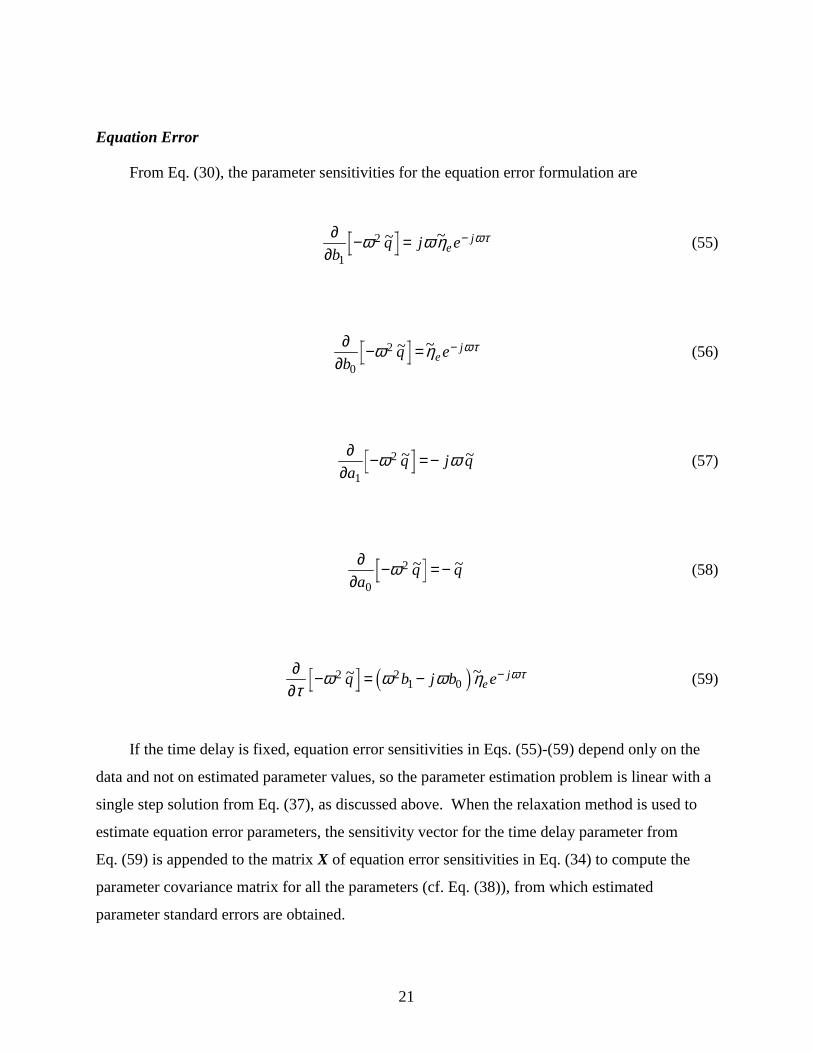
From Eq. (30), the parameter sensitivities for the equation error formulation are
∂∂
− = −b
q j eej
1
2ω ω η ωτ~ ~ (55)
∂∂
− = −b
q eej
0
2ω η ωτ~ ~ (56)
∂∂
− = −a
q j q1
2ω ω~ ~ (57)
∂∂
− = −a
q q0
2ω ~ ~ (58)
∂∂
− = − −τ
ω ω ω η ωτ2 21 0
~ ~q b j b eej3 8 (59)
If the time delay is fixed, equation error sensitivities in Eqs. (55)-(59) depend only on the
data and not on estimated parameter values, so the parameter estimation problem is linear with a
single step solution from Eq. (37), as discussed above. When the relaxation method is used to
estimate equation error parameters, the sensitivity vector for the time delay parameter from
Eq. (59) is appended to the matrix X of equation error sensitivities in Eq. (34) to compute the
parameter covariance matrix for all the parameters (cf. Eq. (38)), from which estimated
parameter standard errors are obtained.

22
Comparison of output error sensitivities in Eqs. (42)-(46) with the corresponding equation
error sensitivities in Eqs (55)-(59) reveals that the sensitivities differ only by a factor of
1 21 0− + +ω ωa j a3 8 , as long as the parameters used to compute the output error sensitivities
produce a model pitch rate that matches the measured pitch rate. It follows that when the
parameters used to compute output error sensitivities also produce an output error cost close to
the minimum, the convergence behavior of equation error and output error should be similar.
When the parameter values used to compute output error sensitivities are farther from the values
for minimum output error, the output error sensitivities are misleading, sometimes to the extent
that the output error parameter estimation does not converge or converges to non-physical
values. In some cases, the output error method fails to produce realistic values for the
parameters even when started at values considered close to the values for minimum output error,
e.g., equation error estimates. It appears that the interplay between the frequency content in the
measured input/output data and the sequence of parameter estimates inherent in nonlinear
parameter estimation (cf. Eqs. (20) and (21)) can produce sensitivities that never direct the
optimizer to a realistic solution. Some of these issues are demonstrated using simulation
examples described later.
LOES MODELING ISSUES
Neither output error nor equation error parameter estimation in the frequency domain
require integration, because all time derivatives become multiplications in frequency. Bias
parameters are avoided in both techniques by detrending the time domain data and selecting
2π T as the lowest frequency for the Fourier transformation, where T is the time length of the
data record. There are no ratios of spectral estimates to compute, as required for a Bode plot.
The data has simply been transformed from the time domain to the frequency domain for
analysis. For most practical flight test data analysis, the number of data points in the frequency
domain is much less than in the time domain m N<<1 6 , so that data analysis in the frequency
domain involves many fewer data points. This advantage is gained by using the arbitrary
frequency, high accuracy Fourier transform21. The result is more efficient calculation and faster
parameter estimation because only chosen frequencies in the frequency band of interest are used
for the Fourier transformation and data analysis. Also, in the frequency domain, the estimated

23
parameter covariances are automatically corrected for the spectral content of the residuals15,16,19.
Transformation to the frequency domain allows multiple maneuvers to be analyzed
simultaneously, thus enhancing the information content in the data used for modeling. The main
disadvantage for parameter estimation in the frequency domain is that a time domain simulation
must be carried out using the identified model to check the model fit to measured outputs in the
time domain.
An effective approach for LOES model identification is to use the equation error solution to
provide starting values for the output error problem. This two stage technique retains the
favorable statistical properties of the output error parameter estimates18, and avoids convergence
problems that result when the starting values of the parameters are far from the minimum, which
means the output error sensitivities (cf. Eqs. (42)-(46)) can be misleading. Using the equation
error formulation with fixed τ means that no starting values are needed, except for τ . A good
starting value for τ is 0.1 sec in nearly all cases. Since the equation error estimate for τ is
found using a line search with the other parameters fixed, each equation error parameter
estimation is a linear parameter estimation problem, which is solved in a single step. Figures 1
and 2 show that the equivalent time delay parameter τ is one of the most troublesome in terms
of parameter correlations. Fixing the value of τ in each step of the equation error parameter
estimation therefore makes each step toward the solution both fast and well-conditioned. In
many cases, a short iterative output error parameter estimation using the equation error parameter
estimates as starting values is a simple operation, because the parameter estimates from the
equation error solution are very close to the final parameter estimates using output error. Later
simulation examples explore this further.
Another option available to improve closed loop LOES modeling is to use more output
measurements. This improves the parameter estimation, because the ratio of information to
unknown parameters increases, assuming the experiment was designed well.
Aircraft longitudinal short period dynamics involve angle of attack α , in addition to pitch
rate q, and this fact can be used advantageously in LOES model identification. From
Eqs. (13)-(15), the longitudinal LOES transfer function models are

24
~
~αη
τ
e
sb e
s a s a=
+ +
−1
21 0
(60)
~~q b s b e
s a s ae
s
η
τ=
++ +
−1 02
1 0
1 6(61)
The LOES model for incremental z body axis acceleration at the c.g. is
~~
~
~~~
~
~a V
gs
q V
gL
V
g
b e
s a s az
e
o
e e
o
e
os
ηαη η
αηα
τ= -
���
��� = - =-
+ +
���
���
-
02
1 0(62)
The LOES ~ / ~q eη transfer function model in Eq. (61) can be identified at the same time as either
the ~ / ~α ηe model in Eq. (60) or the ~ / ~az eη model in Eq. (62).
Flying qualities specifications were historically developed for conventional airplanes,
where stick deflection commands angle of attack29. It therefore makes sense to include the angle
of attack response in estimating LOES models for comparison with the flying qualities
specifications, which are based largely on flight testing of conventional airplanes. The angle of
attack measurement is normally from a vane which is subject to systematic errors, particularly at
high angles of attack. These systematic errors can be estimated using data compatibility
analysis30. The linear acceleration at the c.g. would be preferred when the angle of attack
measurement is suspect, for example, because of the position of the sensor in the flow field.
The transfer function models of Eqs. (60)-(62) each involve only a single output
measurement. In contrast, if a state space model structure like Eq. (11) is chosen, each equation
in the state space model involves more than one state. The state space model of Eq. (11)
therefore requires both pitch rate and angle of attack measurements for the equation error
formulation.
The equation error and output error formulations in the frequency domain differ in how the
sensitivities are computed, i.e., using measured quantities for equation error sensitivities and

25
computed model outputs for output error sensitivities. In addition, the equation error method
minimizes the equation error, which involves matching state derivatives, rather than matching
outputs, as in the output error method. The method for computing the weighting matrix is the
same for both methods, except for the fact that the equation error applies to time derivatives of
the states rather than the outputs, as for the output error method (cf. Eqs (24)-(25) and (40)-(41)).
Another approach for ameliorating parameter correlation and insensitivity problems is to fix
one or more parameters at specific a priori values. Frequently the 12
Tθ parameter in Eq. (1)
(equivalently, Lα in Eq. (14)) is set equal to the open loop Lα stability derivative, i.e.,
12
T Lθ α≡ 1 6bare airframe 1,3,5. The reasoning behind this a priori choice of 1
2Tθ is that if the
effects of the higher order control system dynamics and nonlinearities are taken up in the
equivalent time delay, then classical linear flight dynamic analysis can be used to show that the
LOES zero location should be roughly the same as open loop Lα , cf. Eqs. (1) and (14).
Figures 5 and 6 give parameter correlation information for the output error formulation and
the transfer function model of Eq. (1), in the same format as before, using equivalent parameter
values from Eq. (48), with the same impulse input. Figures 5 and 6 show that the 12
Tθ
parameter has the largest number of strong correlations, including both high and low frequency
correlations, and is correlated in some way with every other model parameter. Fixing the value
of 12
Tθ therefore greatly improves parameter identifiability.
Unfortunately, no claim can be made concerning the satisfaction of Mil-Spec requirements
related to parameter 12
Tθ when it is fixed a priori, rather than estimated from measured flight
test data. In addition, examination of Eq. (1) and Figure 6 reveals that if 12
Tθ is fixed in the
numerator of Eq. (1) to an incorrect value, then any other parameter can be badly biased,
depending on the frequency content of the input. The following excerpt from the Mil-Spec1
relates directly to this discussion, showing the effects of parameter correlation on parameter
estimates and how fixing the value of 12
Tθ can change the modeling results significantly:

26
"An example of the differences with 12
Tθ fixed and free is seen in table XII (taken from
MDC Rpt. A6792 fits of the AFFDL-TR-70-74 data). It can be seen that substantial
differences in all the effective parameters exist between the 12
Tθ -fixed and -free fits.
Hence the dilemma is not a trivial one."a
TABLE XII. Examples of variations in LOES parameters with 12
Tθ fixed and freeb
1 Tθ2ω sp ζ sp τ e
CONFIGU-
RATIONFIXED FREE FIXED FREE FIXED FREE FIXED FREE
1A 1.25 0.43 3.14 2.54 0.39 0.65 0 0.020
1G 1.25 176.0 0.78 1.55 0.74 1.07 0.185 0.043
2H 1.25 4.08 2.56 3.80 0.80 0.52 0.126 0.098
4D 1.25 5.25 3.47 4.61 0.58 0.23 0.169 0.111
Deterministic modeling error, such as high order control system dynamics and
nonlinearities, cannot be restricted to a single free parameter, e.g., the equivalent time delay.
Some of the deterministic modeling error will be taken up in the 12
Tθ parameter estimate (and
the other parameter estimates as well), which means that an adequate LOES model will need a
value for 12
Tθ that is different from the open loop value of Lα . Movements in the free
parameters can and will account for deterministic modeling error to some extent when used in
the LOES modeling context. Assuming the input is sufficiently rich, when one or more of the
parameters is fixed to a value different from what would be chosen with all parameters free, then
the estimation algorithm adjusts the remaining parameters to compensate for the parameter(s)
whose freedom has been taken away. Naturally, the free parameters chosen for this task by the
a Military Standard – Flying Qualities of Piloted Aircraft, MIL-STD-1797A, January 1990,(Ref. [1]), p. 176.
b ibid, p. 176.

27
optimizer are those most correlated with the frozen parameter(s). Later simulation examples
demonstrate these effects.
When a model parameter is fixed, its standard error is assumed to be zero (or very small),
indicating a secure knowledge of the parameter value before analyzing any data from the
experiment. For the case of fixing Lα , the difficulty arises because this parameter cannot be
assigned the distinct role of accounting for only the open loop linear effect when used in the
LOES modeling context, and therefore its a priori value is inconsistent with a very small
standard error. High order control system dynamics and nonlinearities must also be partially
accounted for by movement of the Lα parameter in conjunction with the other free parameters.
If it were possible to assign a distinct role to a particular parameter in the LOES model, and
an accurate a priori value could be determined, then fixing that parameter to the a priori value
would be valid and the conditioning for remainder of the LOES model parameter estimation
problem would be improved. Such an opportunity exists for the equivalent time delay parameter,
as described next.
Some flight test investigations aimed at correlating low order equivalent systems with pilot
ratings8-10 implement the equivalent time delay as a pure delay between the stick and the control
surface deflection. It can be inferred from the preceding discussion that when all LOES model
parameters are free, the estimated equivalent time delay parameter is not an estimate of any real
pure time delay but rather some combination of the pure time delay plus other dynamical effects.
Therefore, the estimate of the equivalent time delay parameter from flight test data can be
different from the quantity that has been correlated with pilot opinion through flight test.
In order to remedy the situation, it is proposed that the role of the equivalent time delay
parameter be assigned to that used in correlations with pilot opinion through flight research. The
equivalent time delay is estimated as the pure time delay from stick deflection to control surface
deflection. Figure 7 is an expanded view of longitudinal stick deflection and the corresponding
measured stabilator response near the initiation of a maneuver flown on the NASA F-18 HARV.
The pure time delay from stick deflection to control surface can be estimated accurately using a
time domain procedure described in the Mil-Spec and illustrated in Figure 7. Point A is the point
of departure from the trim value for the longitudinal stick deflection. Point C is the effective
departure from trim for the stabilator, which is computed as the projection back to the stabilator

28
trim value (normalized to zero in Figure 7) from the point with maximum slope for the initial
stabilator deflection, point B, using the local slope at point B. The estimated pure time delay is
the distance between points A and C on the time axis.
Pilot inputs and the control surface deflections are generally measured with very low noise
levels, as evidenced by Figure 7, which is unfiltered measured flight test data from the F-18
HARV. The initial longitudinal stick deflection from a steady trim condition must be used,
because of subsequent feedback control and aircraft dynamic response. Square wave input
forms, such as those used in the optimal input design technique of Ref. [28], help the accuracy of
the time delay estimation because of the abrupt input amplitude change from trim. Equivalent
time delay estimated in this way corresponds directly to the time delay correlated with pilot
ratings in the literature8-10, including the Mil-Spec1.
In practice, sometimes more than one control surface responds to pilot inputs, due to the
action of the control system. In this case, it is reasonable to compute an average of the pure time
delay values estimated for each of the control surfaces that move significantly in response to the
pilot input, and assign this average value as the equivalent time delay. If control surface
effectiveness values are known, it may be more accurate to use a pure time delay average
weighted by the relative effectiveness values for the control surfaces that move significantly in
response to the pilot input.
At another level of sophistication, equivalent time delay estimated from control time
histories, as shown in Figure 7, could be introduced as an a priori value of the time delay
parameter for output error parameter estimation in the frequency domain. Reference [15]
outlines how this can be done for any model parameter. A reasonable uncertainty for the a priori
value of the time delay estimated in this way would be ± ∆t 2 . This approach removes
parameter correlations by using an a priori estimate for the equivalent time delay that is
consistent with the time delay that has been correlated with pilot opinion in flight tests.
Finally, the preferred approach is to estimate all model parameters, including equivalent
time delay, from measured input/output data using the equation error or output error methods
described above. When parameter correlation difficulties occur, however, the technique outlined
here can be used to find an independent estimate of the equivalent time delay, which can then be
used to improve the conditioning of the complete parameter estimation problem.

29
III. Simulation Examples
The first simulation example is a Single-Input, Single-Output (SISO) longitudinal case,
using a longitudinal stick input measured in flight on the F-18 HARV and shown in Figure 8.
This pilot input was chosen because of its wide-band frequency content centered near the natural
frequency of the simulation model; however, the input was not optimized in any way for this
work. Simulated data was generated by applying this longitudinal stick input to the model of
Eq. (2) using parameter values from column 2 of Table 3. Since this first example has no
modeling error, it is not a LOES modeling case. The example was included to demonstrate the
parameter estimation algorithms in the frequency domain and to study some parameter
correlation issues. Sample rate for the time domain data was 50 Hz. White Gaussian noise was
added to the simulated pitch rate output so that the signal-to-noise ratio was approximately 5 to
1. The simulated noisy pitch rate measurement is shown in Figure 9.
Parameters in the model of Eq. (2) were estimated from the simulation input and output
data using equation error and output error in the frequency domain, as described above. The
Fourier transform was done at frequencies evenly spaced at 0.1 rad/sec intervals for
01 10. rad / sec rad / sec≤ ≤ω , giving 100 data points in the frequency domain for each signal.
The output error method used the equation error parameter estimates as starting values. The
equation error method did not require starting values, except for the equivalent time delay
parameter τ , for which the starting value was 0.1 sec. The parameter estimation results given in
Table 3 indicate that the equation error method gave parameter estimates that matched the true
values within approximately ±1 standard error, indicating that the input was sufficiently rich to
allow accurate estimation of the LOES model parameters. The output error method, starting
from the equation error parameter estimates and using the same data, improved the accuracy of
every parameter estimate and lowered every standard error. The standard errors from the output
error method were still representative of the true accuracy of the output error parameter
estimates. Similar results were seen when the simulation example was repeated for numerous
realizations of the Gaussian noise sequence added to the simulated pitch rate.
The state space model parameterization of Eq. (14) was also used for the output error
parameter estimation. The results obtained were similar both in terms of the proximity of the

30
parameter estimates to the true values, and in the fact that the parameter standard errors correctly
represented the accuracy of the parameter estimates.
A random low frequency or high frequency input can be generated by passing a Gaussian
white noise sequence through a filter. A low frequency input was generated in this way using a
5th order Butterworth low pass filter with cut-off frequency 0.3 Hz. The result is shown in
Figure 10. The input power spectrum in Figure 11 indicates that the filtering successfully
removed frequency components above 0.3 Hz. Simulated pitch rate response using the same
model as before with 20% white Gaussian measurement noise added is plotted in Figure 12.
Table 4 contains results from the parameter estimation. The third column of Table 4
contains equation error parameter estimates and standard errors. Column 4 of Table 4 shows
results from output error parameter estimation using the equation error parameter estimates for
starting values. The same frequencies as in the previous example were used for the Fourier
transforms. Again, the output error method improved the results both in terms of parameter
accuracy and smaller standard errors. Although the equation error estimates were less accurate,
the associated standard errors properly reflected this. Similarly, the standard errors from the
output error method correctly quantified the true parameter accuracy. The fifth column of Table
4 shows the results obtained from output error parameter estimation when the starting values of
the parameters were not as good as the equation error estimates, but still reasonable guesses. In
this case, the output error estimation converged to very inaccurate parameter values. Standard
errors were badly inaccurate and therefore did not reflect the true parameter accuracy. This
behavior was the result of the numerous high parameter correlations for low frequency inputs
using the output error formulation and misleading sensitivities, as discussed above.
Other similar simulation runs were carried out, using low frequency inputs from different
filtered noise sequences and different output measurement noise sequences. Equation error
always produced an answer. The proximity of the equation error parameter estimates to the true
parameter values correlated well with the time domain match of measured output to model
output using the equation error parameter estimates. When the equation error time domain
match was not good, the subsequent output error estimation usually did not converge when
started from the equation error parameter estimates. This suggested that the time domain fit

31
using equation error parameters could be used as an indication of the suitability of the equation
error parameter estimates as starting values for the output error parameter estimation.
In this example, a useful metric for a reasonable time domain model fit to the data was:
Jz y z y
y y
rms v
rms y
T
T=
− −= <
1 6 1 6 1 61 6 0 4. for a good fit (63)
Since the random noise component of z comprised 20% of rms y1 6 , the cutoff value of 0.4
given for the time domain fit means the root mean square (rms) of the deterministic model
mismatch was roughly equivalent to that of the non-deterministic model mismatch. The above
metric worked well for this example, but cannot be recommended for general application without
further study.
As long as the equation error time domain match was reasonable (as defined above), the
subsequent output error parameter estimation converged and produced improvement in the
results similar to that shown in Table 3 and columns 3 and 4 of Table 4. Similar statements
apply for high frequency inputs, which were also tested using the same simulation, with similar
results.
Table 5 contains parameter estimation results for the same simulation using the flight test
input of Figure 8 and the same output noise level, but using both α and q measurements in the
data analysis, with the same frequencies for the Fourier transform. Figure 13 shows the
simulated measured outputs. The pitch rate plot in Figure 13 is identical to Figure 9. Compared
to the results in Table 3 for the same simulation and parameter estimation method, but using only
the q measurement, the results in Table 5 show that the additional measurement improved
parameter accuracy and lowered standard errors for both the equation error and output error
methods. As in the single output case, the output error method converged to reasonable
parameter estimates when the starting values were relatively close to the true values. The
equation error method again provided good starting values for the output error parameter
estimation, and the proximity of the equation error parameter estimates to the true values
correlated well with the time domain match. State space parameterization using both the α and q

32
measurements for this simulation example produced similar results. In all cases, using either the
equation error or the output error method, the proximity of the estimated parameters to the true
values was accurately represented by the estimated standard errors.
For the multiple output cases, the equation error method converged well using the same
modified Newton-Raphson optimization technique used for the output error cases. This
optimization technique moves all unknown parameters at the same time. For the single output
equation error case, it was necessary to use the relaxation method, wherein the equivalent time
delay was estimated while the linear model parameters were fixed, and vice versa. Multiple
measured outputs provided enough additional information in the data that the relaxation
technique was not required for the equation error method in the multiple output case.
The output error method using the relaxation method for equivalent time delay estimation
did not improve convergence behavior compared to the output error method using modified
Newton-Raphson optimization. The output error method required starting values from the
equation error method in conjunction with modified Newton-Raphson optimization to converge
reliably in all cases.
Returning to the SISO case, the next example introduces deterministic modeling error,
which is the usual situation for LOES modeling. The high order system transfer function was:
~~
.
.
.
.
.
qA s C s
s
ss
s ss
eη= =
+
+ ���
��� +
�!
"$##
+�!
"$# + �
����� +
�!
"$##
1 6 1 6 1 6
1 6 1 6
125 1
4 92
0 74 9
1
1
21
632
0 7563
12
2
2
2
(64)
where
A ss
ss
1 6 1 6
1 6
=+
+ ���
��� +
�!
"$##
125 1
4 92
0 74 9
12
2
.
.
.
.
(65)

33
was the transfer function for the open loop short period dynamics of the aircraft, and
C ss s
s
1 6
1 6
=
+�!
"$# + �
����� +
�!
"$##
1
21
632
0 7563
12
2.
(66)
was the transfer function for the control system dynamics. The high order system in Eq. (64) is
configuration 2H from Ref. [12], quoted in Refs. [1] and [3]. In Ref. [12], the longitudinal
dynamics in Eq. (64) (and many other high order dynamic systems) were simulated in-flight and
rated by test pilots using the Cooper-Harper scale for a flying qualities evaluation task. LOES
parameter estimation results (given for configuration 2H in the Mil-Spec table above, cf. Theory
section) were obtained using a least squares fit to Bode plot magnitude and phase information for
the high order system over the frequency range 0.1 to 10 rad/sec, using the cost function:
J q qLS i hos i LOESi
m
i hos i LOES= − + −
=∑ 20 20 0 017510 10
2
1
2log ~ log ~ .ω ω ϕ ω ϕ ω1 6 1 64 9 1 6 1 63 8 (67)
For the present example, the same longitudinal pilot input shown in Figure 8 was applied to
the high order system of Eq. (64), and the output was corrupted with 20% white Gaussian noise.
The same frequencies as before were used for the data analysis.
Table 6 shows parameter estimation results. The second column of Table 6 contains the
equation error parameter estimation results and corresponding standard errors. Column 3
contains the output error results using the same data with starting values from the equation error
results. Column 4 contains output error results with 12
Tθ fixed at 1.25 for the same data. The
fifth and sixth columns of Table 6 are results from the Mil-Spec table quoted in the last section,
converted to the parameterization of Eq. (2) for comparison purposes. For the results in columns
5 and 6 of Table 6, the LOES gain parameter was set to one (the true value for the high order
system), and therefore was not estimated. Standard errors for the estimated parameters in
columns 5 and 6 of Table 6 were not included in Refs. [1] or [12].

34
Output error parameter estimation results using the simulated data with 12
Tθ fixed at 1.25
(column 4, Table 6) were similar to the results in column 5, which were obtained from a least
squares fit of the frequency response magnitude and phase, as described above. This indicates
that the short 16 second time record using the input of Figure 8 had enough information for the
output error estimator to match results from the least squares Bode plot analysis. The Bode plot
for the high order system in Eq. (64), which comprised the data for the results in columns 5 and 6
of Table 6, corresponds to a perfect spectral estimation of the dynamic response. In practice,
extended sine sweep inputs would be necessary to generate something close to the frequency
response data used for the Bode plot least squares fit. In addition, the gain parameter was set to
one (the true value) for the Bode plot analysis, and therefore was not estimated. This helps the
parameter estimation, since the LOES gain value is exactly correct and there is one fewer
unknown parameter to be estimated. In practice, the LOES gain parameter is unknown and must
be estimated from the data.
The third row from the bottom of Table 6 shows the ratio of flying qualities level predicted
from the estimated parameters and the Mil-Spec, to the actual pilot ratings for this high order
system in flight, taken from Ref. [12]. The Bode plot analysis required a fixed and accurate
value of 12
Tθ to correctly predict the handling qualities rating. The output error parameter
estimates in column 3 of Table 6 correctly predicted actual pilot flying qualities ratings using
only the pilot longitudinal stick and pitch rate data from a short maneuver.
The last two rows of Table 6 give some insight into the modeling. Cost values using
Eq. (67) for frequency ranges 0.1 to 10 rad/sec and 1.5 to 6 rad/sec were computed for all the
parameter estimation results, using a constant 0.1 rad/sec frequency spacing. Most of the power
(88%) for the input of Figure 8 lies in the frequency range 1.5 to 6 rad/sec. The methods that
used simulation data (columns 2 through 4) gave low cost values for this frequency range, with
the output error method giving the lowest cost. For the full frequency range, the least squares
Bode plot method with all parameters free gave the lowest cost value, because the optimization
problem was formulated that way. However, the LOES model parameters estimated using this
method did not correctly predict flying qualities level (cf. Table 6, column 6). As noted above,
the Bode plot method required a fixed and accurate a priori value of the LOES 12
Tθ parameter
to correctly predict the flying qualities level in this case. In practice, accurate a priori values for

35
the LOES model 12
Tθ parameter are not available, because model parameters must include both
bare airframe and control system effects in the LOES context.
Previous work1 on pilot sensitivity to variations in the dynamic aircraft response as a
function of frequency have shown that the pilot is most sensitive to changes in dynamics near the
crossover frequency. It is therefore reasonable to identify the LOES model based on data in this
region to accurately predict flying qualities ratings from the pilot. This example demonstrates
that data from short flight test maneuvers with input energy near the crossover frequency of the
high order system can be used with the methods described in this work to identify accurate
LOES models that successfully predict pilot ratings from flight.
Model parameters in the LOES context do not have “true” values, because the structure of
the model is incorrect by assumption. The main requirements are that the identified LOES
model, whatever its parameter values, accurately represents the data with parameter values that
have good identifiability (indicated by low standard errors). Such models predict flying qualities
well. Parameter values for adequate LOES modeling are therefore not unique, and could easily
change with the frequency range of the modeling, for example. Parameter standard errors in the
LOES modeling context are more indicative of parameter identifiability, and should not be
interpreted as a measure of the accuracy of the LOES parameter estimate relative to some “true”
value.
The last simulation example includes deterministic modeling error that interacts
significantly with the techniques used for LOES modeling. Specifically, this example
investigates the “galloping Lα ” problem. The true high order system transfer function was:
~~
.
.
.
. .
.
qA s C s
s
ss
s ss
eη= =
+
+ ���
��� +
�!
"$##
+�!
"$# + �
����� +
�!
"$##
1 6 1 6 1 6
1 6 1 6
125 1
2 22
0 692 2
1
1
0 51
632
0 7563
12
2
2
2
(68)
where

36
A ss
ss
1 6 1 6
1 6
=+
+ ���
��� +
�!
"$##
125 1
2 22
0 692 2
12
2
.
.
.
.
(69)
was the transfer function for the open loop short period dynamics of the aircraft, and
C ss s
s
1 6
1 6
=
+�!
"$# + �
����� +
�!
"$##
1
051
632
0 7563
12
2.
.(70)
was the transfer function for the control system dynamics. The high order system in Eq. (68) is
configuration 1G from Ref. [12], quoted in Refs. [1] and [3]. This is also one of the cases
included in the table excerpted from the Mil-Spec in the last section.
The same longitudinal pilot input shown in Figure 8 was applied to the high order system of
Eq. (68), and the output was corrupted with 20% white Gaussian noise. The same frequencies as
before were used for the data analysis.
Table 7 shows parameter estimation results for this example in the same format used for
Table 6. The second column of Table 7 contains the equation error parameter estimation results
and corresponding standard errors using the pitch rate output and longitudinal stick input.
Column 3 contains the output error results using the same data with starting values from the
equation error results. Column 4 contains output error results using transfer function models and
both the pitch rate and angle of attack outputs. The fifth and sixth columns of Table 7 are results
from the Mil-Spec table quoted in the last section, with the parameters converted to the
parameterization in Eq. (2) for comparison purposes. The latter results were obtained using a
least squares fit to Bode plot data, in the same manner described above for case 2H.
The results in column 6 of Table 7 show the characteristic “galloping Lα ” problem, namely
that Lα is estimated as a very large value L b b Tα θ= =0 1 123 8 . The results in column 3 of
Table 7, which were obtained from simulated data using the input of Figure 8, show a close
similarity to the results in column 6 of Table 7, which were generated from a least squares fit of a

37
perfect Bode plot for the high-order system pitch rate response. The “galloping Lα ” problem
has therefore been reproduced using the data from the 16 sec simulated maneuver.
The last two rows of Table 7 show cost values using Eq. (67) for the pitch rate only, over
frequency ranges 0.1 to 10 rad/sec and 1.5 to 6 rad/sec, using a constant 0.1 rad/sec frequency
spacing. Most of the power (88%) for the input of Figure 8 lies in the frequency range 1.5 to
6 rad/sec. Results in column 2 of Table 7 show that the equation error parameter estimation
results are reasonable, and the costs are comparable to the output error cases in columns 3 and 6,
which used only the pitch rate output with all parameters free. Reasonable parameter estimation
results were also obtained in column 4 of Table 7, where the output error method was used with
both the angle of attack and pitch rate outputs. For this method, the costs are significantly higher
than the others, indicating that some trade-off in fit error between the two outputs occurred in the
output error minimization. The standard errors in column 3 of Table 7 indicate that the output
error parameter estimates with the “galloping Lα ” characteristic had poor identifiability and
were very inaccurate. In contrast, the standard errors were low for the equation error results in
column 2 and the output error results using both angle of attack and pitch rate in column 4,
indicating that the estimated LOES model parameters were accurate with good identifiability.
The standard errors computed for all the methods described in this work gave important
information regarding the adequacy of the LOES model parameters, even when deterministic
modeling error was present. The time domain matches of model output pitch rate to measured
pitch rate were similar and very good for all the LOES parameter estimation results given in
Table 7.
In all cases, the third row from the bottom of Table 7 indicates that the predicted flying
qualities matched the pilot ratings from flight. In the cases with “galloping Lα ” (columns 3 and
6, Table 7), level 3 flying qualities was correctly predicted only because the “galloping Lα ”
parameter caused a level 3 flying qualities prediction. The remaining parameter values would
predict level 1 flying qualities. In the case with the best LOES model parameter accuracy
(column 4 of Table 7), flying qualities level 3 was predicted from two of the criteria specified in
the Mil-Spec.

38
This example demonstrated that the output error correlation problem that manifests itself as
a “galloping Lα ” can be solved using an equation error method with the same data, or an output
error method with an additional output measurement. The corresponding LOES modeling results
in columns 2 and 4 of Table 7 are not in agreement, yet both models contain parameter values
with low standard errors, and both predict flying qualities correctly. This demonstrates that the
adequate LOES model is not unique. The LOES models in columns 2 and 4 of Table 7 were
generated from different parameter estimation formulations, with an additional output
measurement used in the output error case.

39
IV. Flight Test Examples
Flight test data from the NASA F-18 HARV was used to demonstrate the LOES modeling
techniques described above. The F-18 HARV is an F/A-18A airframe which was modified
extensively for high angle of attack dynamics and control research, as part of the NASA High
Alpha Technology Program. Modifications included thrust vectoring, a research-quality
instrumentation system, additional emergency systems, forebody strakes, and a research flight
control computer capable of implementing multiple control laws. More details on the F-18
HARV are available in Ref. [31].
The first example involved longitudinal tracking at approximately 40 deg angle of attack.
At this high angle of attack condition, the parameters in the fixed LOES model structure must
characterize both the control system dynamics and the open loop airplane dynamics, which are
typically nonlinear. The LOES modeling task is therefore very challenging.
Data for this example was taken from 3 identical tracking task maneuvers on the
F-18 HARV using the same control law, but flown by different pilots on different days. The
upper plots of Figures 14-16 show the longitudinal stick deflection for a 20 second time slice
from each maneuver. The lower plots in Figures 14-16 indicate the measured pitch rate response
with a solid line, and the identified LOES model fit with a dashed line. The LOES model
identification was done using the SISO model of Eq. (2), and equation error in the frequency
domain with relaxation applied to the time delay estimation, as described above. The fit of the
LOES model to the data was excellent, considering the high angle of attack, the short time length
of data, and the fact that only the measured pitch rate output was used.
Table 8 contains the LOES model parameter estimates and standard errors for the 3
maneuvers depicted in Figures 14-16. The estimated values of the gain parameter b1 and the
damping parameter a1 show statistical agreement among the 3 maneuvers, meaning that the 95%
confidence intervals (parameter estimate ±2 standard errors) overlap. The other parameters,
b a0 0, , , and τ do not agree in this way. At the bottom of Table 8, values for numerator zero
parameter 12
Tθ , short period damping ζ sp , and natural frequency ω sp , based on the LOES
parameter estimates, are listed. The last row of Table 8 contains the flying qualities levels given
by the pilot in flight, compared to values computed from the Mil-Spec1 using LOES model

40
parameters estimated from the flight test data. LOES modeling is dimensional, and therefore
includes flight condition and mass properties. Table 9 contains the pertinent values for each
maneuver.
Although the airplane, control law, and approximate flight condition were the same, three
different pilots rated the same tracking task as level 1, 2, and 3. This interesting phenomena was
in fact the reason that these maneuvers were chosen for analysis. LOES modeling results in
Table 8 indicate that the pilots, who were all experienced test pilots, actually gave ratings that
were consistent with the response of the aircraft indicated by the data. For the dynamic response
that each pilot experienced, his flying qualities ratings were consistent with those predicted by
the Mil-Spec and the LOES model identified from the measured data.
The flight condition and mass property differences shown in Table 9, though not negligible,
were not considered sufficient to account for the different pilot ratings. Another possible
explanation for the different pilot ratings could be that in this nonlinear flight regime, the
difference in how each pilot perceived the flying qualities was related to how he flew the aircraft.
Figure 17 shows that the power spectra of the longitudinal stick deflections for each pilot were
quite different during the 20 second tracking tasks shown in Figures 14-16. The pilot for
Maneuver 376d (upper plot in Figure 17) flew the airplane with predominantly low frequency
inputs, and rated the airplane level 1. The pilot for Maneuver 321e (middle plot in Figure 17)
flew the airplane with a wide spectrum of input power, fairly equally distributed across the
LOES modeling frequency range of 0.016–1.6 Hz, and rated the airplane level 2. The pilot for
Maneuver 320j was a high frequency, high gain pilot (note the vertical scale difference in the
lower plot of Figure 17). This caused a large amount of control surface rate limiting, which is
reflected in the estimate of equivalent time delay for this maneuver in Table 8. This pilot rated
the airplane level 3. Based on this analysis, it is possible to conjecture that the ratings the pilots
gave were in fact consistent with the Mil-Spec guidelines, and that the widely different ratings
were the result of the manner in which the airplane was flown to accomplish the task.
The maneuvers were flown at high angle of attack, where the aerodynamics are known to
be nonlinear, and the control surface deflections and rates can reach hard limits. Nonlinear
dynamical system response is known to be sensitive to input frequency and amplitude, and the
LOES model is largely a linear approximation to a nonlinear system in this case. It seems

41
reasonable that the LOES model would change significantly depending on the amplitude and
frequency range of the input when the underlying physical system dynamics are nonlinear.
Due to the nature of the tracking task, the flight test data used for the LOES modeling was
concentrated in a frequency band around the pilot crossover frequency. The LOES modeling
technique therefore identified the best LOES model for this frequency band only, since the
identification was based only on flight test data from each tracking maneuver. The Mil-Spec
guidelines, which were developed at low angle of attack, translated well to this high angle of
attack case where the LOES identification was limited to a frequency band near the pilot
crossover frequency. This result is in consonance with empirical information in the Mil-Spec
showing that a good LOES model must closely match the aircraft closed loop dynamics in the
vicinity of the pilot crossover frequency (cf. Figure 15, p. 181, Appendix A in Ref. [1]). The
high accuracy LOES identification methods outlined in this report made this analysis possible
with very little computational effort.
The last example is a Multiple-Input, Multiple-Output (MIMO) LOES modeling problem.
Closed loop lateral/directional dynamics of the F-18 HARV at 45 deg angle of attack were
modeled based on measured data from a 24 second maneuver, using the LOES model state space
formulation:
&
&
&
&
cos
tan
β
φ
β
φ
η τη τ
β
β φ
β
η η
η η
η η
p
r
Y Y Yg
VL L L L
N N N
p
r
Y Y
L L
N N
t
t
p ro
o
p r
p r
o
r r
a a
r a
r a
r a
�
!
"
$
#####=
�
!
"
$
#####
�
!
"
$
####+
�
!
"
$
####−−
�!
"$#
Θ
Θ0
0 1 0 0 0
1 61 6 (71)
The Yr parameter includes the inertial term, and the Lφ parameter is due to the control law,
which in this case was the research flight control law in thrust vectoring (TV) mode. This LOES
modeling problem is challenging because of the short data record available, the high angle of
attack flight condition, and the MIMO model, which contains a relatively large number of
parameters.

42
Figure 18 shows the rudder pedal and lateral stick inputs, which were implemented by the
research flight control computer and were designed to maximize data information content28.
Each input had an independent equivalent time delay parameter. The solid lines in Figure 19
show the measured outputs used in the LOES model identification. The model structure for the
state space system was determined using equation error in the frequency domain, applied
individually to each line of the state space system in Eq. (71), with the time delays fixed at zero.
The final model parameter estimates were determined using output error in the frequency domain
with all parameters free, using equation error starting values. Starting values for the time delay
parameters τ r and τ a were both 0.1 sec. Table 10 contains the state space model parameter
estimates and standard errors. Most parameter standard errors were less than 15% of the
respective nominal parameter estimate.
The dashed lines in Figure 19 show that the model fit to the data was excellent, even at this
high angle of attack flight condition using a LOES model structure to characterize the end-to-end
dynamic MIMO response. Modal parameters are given at the bottom of Table 10. LOES
transfer functions can be computed easily20 from the parameter estimates in Table 10 and the
state space model of Eq. (71). Using the state space model formulation for the LOES model
identification allowed inclusion of important control law parameters Lφ3 8 without violating the
fixed transfer function structure imposed by the Mil-Spec for lateral/directional LOES models.
In addition, the state space model formulation allowed the use of many output measurements to
improve model parameter estimate accuracy. The identified closed loop dutch roll damping is
0.72, which was close to the 0.70 target value for the control law design. Correlations of pilot
ratings with lateral/directional LOES identified from flight test data using the methods described
in this report can be found in Ref. [32].

43
V. Summary
Low Order Equivalent System (LOES) models are low order linear models with input time
delay, used to characterize closed loop aircraft response to pilot inputs. In this work, methods
for accurately identifying LOES models from flight test data were developed and demonstrated.
Data analysis was done in the frequency domain using a high accuracy Fourier transform
with selectable frequency range and resolution. Data analysis in the frequency domain was
chosen because of the equivalent time delay parameter appearing in LOES models, in addition to
computational and practical advantages. Effective output error and equation error parameter
estimation methods were developed, and their properties were examined using sensitivity
analysis and simulation examples. A variety of modeling topics were discussed, including
experiment design implications and data requirements for LOES modeling, model parameter
identifiability and sensitivity analysis, frequency resolution, the “galloping Lα ” problem, and a
method for independent estimation of the equivalent time delay, with interpretation in the LOES
modeling context. Modeling techniques were demonstrated using simulation cases, then applied
to Single-Input, Single-Output (SISO) and Multiple-Input, Multiple-Output (MIMO) closed loop
flight test data from the NASA F-18 High Alpha Research Vehicle.
Flight-determined LOES models are useful in many applications, including control law
design validation, simulation, flying qualities research, aircraft development and specification
compliance, and quantifying dynamic response and flying qualities using flight test data from
flying qualities evaluation tasks.

44
VI. References
1. Military Standard – Flying Qualities of Piloted Aircraft, MIL-STD-1797A, January1990.
2. Hodgkinson, J., LaManna, W.J., and Heyde, J.L., "Handling Qualities of Aircraft withStability and Control Augmentation Systems – A Fundamental Approach", AeronauticalJournal, February 1976, pp. 75-81.
3. Mitchell, D.G. and Hoh, R.H., "Low-Order Approaches to High-Order Systems:Problems and Promises", Journal of Guidance, Control, and Dynamics, Vol. 5, No. 5,Sept.-Oct. 1982.
4. Cooper, G.E., and Harper, R.P. Jr., "The Use of Pilot Rating in the Evaluation ofAircraft Handling Qualities", NASA TN D-5153, April 1969.
5. Hodgkinson, J. and LaManna, W.J., "Equivalent System Approaches to HandlingQualities Analysis and Design Problems of Augmented Aircraft", AIAA paper 77-1122,Atmospheric Flight Mechanics Conference, Hollywood, FL, August 1977.
6. Hodgkinson, J. and Johnston, K.A., "Initial Results of an Inflight Simulation ofAugmented Dynamics in Fighter Approach and Landing", AIAA paper 79-1783,Guidance and Control Conference, Boulder, CO, August 1979.
7. Manning, C.O. and Gleason, D. "Flight Test Results using a Low Order EquivalentSystems Technique to Estimate Flying Qualities", AIAA paper 92-4425-CP,Atmospheric Flight Mechanics Conference, Hilton Head Island, SC, August 1992.
8. Berry, D.T., Powers, B.G., Szalai, K.J., and Wilson, R.J., "In-Flight Evaluation ofControl System Pure Time Delays", Journal of Aircraft, Vol. 19, No. 4, April 1982.
9. Smith, R.E., and Sarrafian, S.K., "Effect of Time Delay on Flying Qualities: AnUpdate", Journal of Guidance, Control, and Dynamics, Vol. 9, No. 5, September-October 1986.
10. Berry, D.T., "In-Flight Evaluation of Incremental Time Delays in Pitch and Roll",Journal of Guidance, Control, and Dynamics, Vol. 9, No. 5, September-October 1986.
11. DiFranco, D.A. "In-flight Investigation of the Effects of Higher-Order Control SystemDynamics on Longitudinal Handling Qualities", AFFDL-TR-68-90, August 1968.
12. Neal, T.P., and Smith, R.E., "An In-Flight Investigation to Develop Control SystemDesign Criteria for Fighter Airplanes", AFFDL-TR-70-74, Vols. I & II, December1970.

45
13. Hodgkinson, J., Berger, R.L., and Bear, R.L., "Analysis of High Order Aircraft/FlightControl System Dynamics Using an Equivalent System Approach", Seventh AnnualPittsburgh Conference on Modeling and Simulation, April 26-27, 1976.
14. Hodgkinson, J., Snyder, R.C., and Smith, R.E., "Equivalent System Verification andEvaluation of Augmentation Effects on Fighter Approach and Landing Flying Qualities,Vols. 1 & 2", AFWAL-TR-81-3116, September 1981.
15. Maine, R.E. and Iliff, K.W., "Application of Parameter Estimation to Aircraft Stabilityand Control - The Output-Error Approach", NASA RP 1168, June 1986.
16. Morelli, E.A. and Klein, V., "Determining the Accuracy of Maximum LikelihoodParameter Estimates with Colored Residuals", NASA CR 194893, March 1994.
17. Klein, V. "Aircraft Parameter Estimation in Frequency Domain", AIAA paper 78-1344,Atmospheric Flight Mechanics Conference, Palo Alto, CA, August 1978.
18. Klein, V., "Maximum Likelihood Method for Estimating Airplane Stability and ControlParameters from Flight Data in Frequency Domain", NASA TP 1637, May 1980.
19. Tischler, M.B., "Frequency-Response Identification of the XV-15 Tilt-Rotor AircraftDynamics", NASA TM 89428, May 1987.
20. McGruer, D., Ashkenas, I., and Graham, D. Aircraft Dynamics and Automatic Control,Princeton University Press, Princeton, New Jersey. 1973.
21. Morelli, E.A. "High Accuracy Evaluation of the Finite Fourier Transform using SampledData", NASA TM 110340, June 1997.
22. Williams, J.N., Ham, J.A., and Tischler, M.B. "Flight Test Manual, RotorcraftFrequency Domain Flight Testing", AQTD Project No. 93–14, U.S. Army AviationTechnical Test Center, Edwards AFB, California. September 1995.
23. Bendat, J.S. and Piersol, A.G. Random Data Analysis and Measurement Procedures,2nd Ed., John Wiley & Sons, New York, NY, 1986.
24. Press, W.H., Flannery, B.P., Teukolsky, S.A., and Vetterling, W.T. Numerical Recipes – The Art of Scientific Computing (FORTRAN Version), Cambridge University Press,Cambridge, UK. 1989.
25. Morelli, E.A., "Practical Input Optimization for Aircraft Parameter EstimationExperiments", NASA CR 191462, May 1993.
26. Cobleigh, B.R. "Design of Optimal Inputs for Parameter Estimation Flight Experimentswith Application to the X-31 Drop Model", MS Thesis, George Washington UniversityJIAFS, NASA Langley Research Center, Hampton, VA, July 1991.

46
27. Morelli, E.A., "Piloted Parameter Identification Flight Test Maneuvers for Closed LoopModeling of the F-18 High Alpha Research Vehicle (HARV)", NASA CR 198268, May1996.
28. Morelli, E.A. "Optimal Input Design for Closed Loop Modeling at High Angles ofAttack", AIAA paper 96-3418, AIAA Atmospheric Flight Mechanics Conference, SanDiego, California. July 1996.
29. Rynaski, E.G., "The Interpretation of Flying Qualities Requirements for Flight ControlSystem Design", NASA CR 177942, August 1985.
30. Klein, V. and Morgan, D.R. "Estimation of Bias Errors in Measured Airplane Responsesusing Maximum Likelihood Method", NASA TM 89059, January 1987.
31. Bowers, A.H., Pahle, J.W., Wilson, R.J., Flick, B.C., and Rood, R.L. "An Overview ofthe NASA F-18 High Alpha Research Vehicle", NASA TM 4772, October 1996.
32. Murphy, P.C., Davidson, J.B., Lallman, F.J., Morelli, E.A., and Messina, M.D., "AnEvaluation of Design Methodology and High Alpha Design Criteria for the ANSERLateral-Directional Control Law", NASA CP-1998-207676 / PT1, Proceedings of theNASA High Angle of Attack Technology Conference, Hampton, Virginia,September 1996.

47
VII. Tables
Table 1 Output Error Longitudinal LOES Parameter Sensitivity Correlations for a Low Frequency (0.1 rad/sec) Input
� �q b1 � �q b0 ∂ ∂q a1 ∂ ∂q a0 ∂ ∂q τ
1 0.037 –0.997 –0.087 –0.990 ∂ ∂q b1
1 0.011 –0.999 0.061 ∂ ∂q b0
1 0.039 0.992 ∂ ∂q a1
1 –0.011 ∂ ∂q a0
1 ∂ ∂q τ
Table 2 Output Error Longitudinal LOES Parameter Sensitivity Correlations for a High Frequency (10 rad/sec) Input
∂ ∂q b1 ∂ ∂q b0 ∂ ∂q a1 ∂ ∂q a0 ∂ ∂q τ
1 0.000 –0.110 0.690 –0.100 ∂ ∂q b1
1 –0.962 –0.223 0.967 ∂ ∂q b0
1 0.000 –0.960 ∂ ∂q a1
1 –0.145 ∂ ∂q a0
1 ∂ ∂q τ

48
Table 3 Longitudinal LOES Modeling Results
Parameter True Value Equation ErrorEstimate
(Std. Error)
Output ErrorEstimate
(Std. Error)
b1 1.000 0.977
(0.037)
1.009
(0.013)
b0 1.000 1.181
(0.370)
1.046
(0.047)
a1 2.000 1.946
(0.256)
1.998
(0.029)
a0 4.000 4.332
(0.695)
3.973
(0.093)
τ 0.100 0.090
(0.007)
0.098
(0.003)
Table 4 Longitudinal LOES Modeling Results for Low Frequency Input
Parameter True Value Equation ErrorEstimate
(Std. Error)
Output ErrorEstimate
(Std. Error)
Output Error Estimate$ . . . .θ 0 05 05 05 1 0 3= T
(Std. Error)
b1 1.000 0.997
(0.616)
0.985
(0.070)
–0.434
(0.018)
b0 1.000 1.519
(0.427)
1.020
(0.037)
0.833
(0.026)
a1 2.000 1.503
(0.741)
1.980
(0.108)
1.136
(0.024)
a0 4.000 5.645
(1.577)
4.040
(0.153)
3.183
(0.067)
τ 0.100 0.208
(0.176)
0.099
(0.022)
–1.031
(0.031)

49
Table 5 Multiple Output Longitudinal LOES Modeling Results
Parameter True Value Equation ErrorEstimate
(Std. Error)
Output ErrorEstimate
(Std. Error)
b1 1.000 0.983
(0.017)
1.005
(0.006)
b0 1.000 0.988
(0.094)
1.010
(0.020)
a1 2.000 1.900
(0.096)
2.001
(0.018)
a0 4.000 4.119
(0.187)
3.998
(0.026)
τ 0.100 0.096
(0.004)
0.100
(0.002)

50
Table 6 Longitudinal LOES Modeling Results for Neal-Smith Case 2H
MDC Bode Plot Estimates
(Ref. [1])
Parameter EquationError
Estimate
(Std. Error)
Output ErrorEstimate
(Std. Error)
All free
Output ErrorEstimate
(Std. Error)
1 1252
Tθ = . 1 1252
Tθ = . All free
b13.188
(0.271)
4.593
(0.185)
5.848
(0.141)5.243 3.539
b017.08
(1.69)
12.39
(0.730)
7.310
*6.554 14.44
a14.198
(0.208)
4.362
(0.096)
4.643
(0.139)4.096 3.952
a016.10
(1.16)
12.27
(0.552)
8.383
(0.193)6.554 14.44
τ 0.076
(0.008)
0.110
(0.005)
0.138
(0.004)0.126 0.098
12
Tθ 5.36 2.70 1.25 1.25 4.08
ω sp 4.01 3.50 2.90 2.56 3.80
ζ sp 0.52 0.62 0.80 0.80 0.52
Pred. FQ level /Pilot FQ level
3/2 2/2 2/2 2/2 3/2
Cost
01 10. ≤ ≤ω73.3 101.0 252.9 163.4 36.3
Cost
15 6. ≤ ≤ω9.0 3.9 5.2 42.1 16.7

51
Table 7 Longitudinal LOES Modeling Results for Neil-Smith Case 1G
MDC Bode Plot Estimates
(Ref. [1])
Parameter EquationError
Estimate
(Std. Error)
q only
Output ErrorEstimate
(Std. Error)
All free
q only
Output ErrorEstimate
(Std. Error)
All free
q and α1 125
2Tθ = . All free
b10.206
(0.054)
9.110e-04
(18.853)
0.618
(0.014)0.487 0.0136
b01.627
(0.208)
2.497
(0.192)
0.596
(0.027)0.608 2.402
a11.989
(0.356)
3.726
(0.269)
1.515
(0.048)1.154 3.317
a02.425
(0.310)
2.938
(0.204)
0.775
(0.024)0.608 2.402
τ 0.111
(0.024)
0.068
(7.539)
0.258
(0.007)0.185 0.043
12
Tθ 7.907 2741.3 0.965 1.25 176.0
ω sp 1.56 1.71 0.88 0.78 1.55
ζ sp 0.64 1.09 0.86 0.74 1.07
Pred. FQ level /Pilot FQ level
3/3 3/3 3/3 3/3 3/3
Cost
01 10. ≤ ≤ω231.5 234.4 3887.0 1933.1 129.1
Cost
15 6. ≤ ≤ω27.8 26.2 398.8 294.9 26.0

52
Table 8 Longitudinal LOES Modeling Results for F-18 HARV Longitudinal Tracking Data
Maneuver 376d Maneuver 321e Maneuver 320j
Parameter Estimate(Standard Error)
Estimate(Standard Error)
Estimate(Standard Error)
b1 0.787
(0.103)
0.745
(0.152)
0.638
(0.041)
b0 1.401
(0.493)
3.346
(0.701)
0.451
(0.203)
a1 3.785
(0.678)
4.371
(0.675)
4.670
(0.314)
a0 15.49
(3.39)
33.84
(4.50)
10.30
(1.53)
τ 0.026
(0.018)
0.042
(0.020)
0.236
(0.018)
12
Tθ 1.78 4.49 0.71
ω sp 3.94 5.82 3.21
ζ sp 0.48 0.38 0.73
Pred. FQ level /Pilot FQ level
1/1 2/2 3/3
Table 9 Flight Conditions for F-18 HARV Longitudinal Tracking Data
Maneuver 376d Maneuver 321e Maneuver 320j
α avg (deg) 37.8 42.6 33.5
qavg (psf) 75.3 64.1 73.6
wavg (lbf) 36,010 38,400 32,930
xcgavg (in)
c = 1152. ft1 6458.8 456.7 459.5

53
Table 10 Lateral/Directional LOES Modeling Results for F-18 HARV Flight Test Data
Maneuver 329r
Parameter Estimate(Standard Error)
Parameter Estimate(Standard Error)
Parameter Estimate(Standard Error)
Yβ–0.073
(0.053)Lβ
–2.85
(0.17)Nβ
0.0282
(0.053)
Yp0.748
(0.024)Lp
–2.55
(0.09)N p
–0.169
(0.053)
Yr–0.690
(0.035)Lr
2.97
(0.15)Nr
–0.478
(0.053)
Yrη
–2.43e-04
(7.30e–05)Lφ
–0.452
(0.025)N
rη2.12e–03
(3.39)
Yaη
–9.11e-03
(1.64e–03)L
rη–5.86e–03
(2.30e–04)N
aη0.0888
(3.39)
Laη
–0.0592
(6.39e–03)τ r
0.0588
(7.94e–03)
τ a0.0125
(0.0104)
Modal Parameters
Spiral Mode Roll Mode Dutch Roll Mode
TS 11.5 TR 1.80 ω DR 1.71
ζ DR 0.72

54
VIII. Figures
-60
-50
-40
-30
-20
-10
0
10
Mag
nitu
de (
dB)
~qb0
~q b1~q a1~qa0
~qt
-400
-300
-200
-100
0
100
200
0.1 1 10
Pha
se (
deg)
Frequency (rad/sec)
Figure 1 Output Error Sensitivities, ~ ~q η from Eq. (2)
-80
-60
-40
-20
0
20
Mag
nitu
de (
dB)
~qLa
~qMa
~q M q
~qt~qM
eh
-400
-300
-200
-100
0
100
0.1 1 10
Pha
se (
deg)
Frequency (rad/sec)
Figure 3 Output Error Sensitivities, ~ ~q η from Eq. (14)
Figure 2 Output Error Sensitivity Correlation Diagram, ~ ~q η from Eq. (2)
Figure 4 Output Error Sensitivity Correlation Diagram, ~ ~q η from Eq. (14)
~qb1
~qb0
~qa1
~qa 0
~qτ
strong high frequency correlation
strong low frequency correlation
strong high frequency correlation
strong low frequency correlation
~qLα
~qMα
~qMq
~qMeη
~qτ

55
-40
-30
-20
-10
0
10
M
agni
tude
(dB
)~q t
~&
q Kq~q
Tq 2
1-
~qspz
~qspw
-500
-400
-300
-200
-100
0
100
0.1 1 10
Pha
se (
deg)
Frequency (rad/sec)
Figure 5 Output Error Sensitivities, ~ ~q η from Eq. (1)
Figure 6 Output Error Sensitivity Correlation Diagram, ~ ~q η from Eq. (1)
-4
-3
-2
-1
0
1
2longitudinal stick (in)stabilator (deg)
1.8 1.9 2 2.1 2.2 2.3 2.4
Time (sec)
A C
Bτ
Figure 7 Equivalent Time Delay Estimation
strong high frequency correlation
strong low frequency correlation
~qspζ
~qTθ21-
~qspω
~qτ
~&
qKθ

56
-0.5-0.4-0.3-0.2-0.1
00.10.20.30.40.5
0 2 4 6 8 10 12 14 16Time (sec)
ηe
(in)
Figure 8 Longitudinal Stick Input
-0.5-0.4-0.3
-0.2-0.1
00.1
0.20.3
0 2 4 6 8 10 12 14 16Time (sec)
ηe
(in)
Figure 10 Low Frequency Longitudinal Stick Input
-15
-10
-5
0
5
10
0 2 4 6 8 10 12 14 16Time (sec)
q
(dps)
Figure 12 Simulated Pitch Rate Output forLow Frequency Longitudinal Stick Input
-10
-5
0
5
10
15
0 2 4 6 8 10 12 14 16Time (sec)
q
(dps)
Figure 9 Simulated Pitch Rate Output
00.0010.002
0.0030.0040.0050.006
0.0070.008
0 0.5 1 1.5 2Frequency (Hz)
Peh
Figure 11 Low Frequency Longitudinal Stick Input Spectrum

57
-4
-2
0
2
4
6
0 2 4 6 8 10 12 14 16Time (sec)
α
(deg)
-10
-5
0
5
10
15
0 2 4 6 8 10 12 14 16Time (sec)
q
(dps)
Figure 13 Simulated Outputs
-0.8
-0.6
-0.4
-0.2
0
0.2
0.4
0.6
0 5 10 15 20Time (sec)
ηe
(in)
Maneuver 376d
-8
-6
-4
-2
0
2
4
6 flightmodel
0 5 10 15 20
q
(dps)
Maneuver 376d
Time (sec)
Figure 14 F-18 HARV Longitudinal Tracking, 45º α.
-0.8
-0.6
-0.4
-0.2
0
0.2
0.4
0.6
0 5 10 15 20Time (sec)
ηe
(in)
Maneuver 321e
-6
-4
-2
0
2
4flightmodel
0 5 10 15 20
q
(dps)
Maneuver 321e
Time (sec)
Figure 15 F-18 HARV Longitudinal Tracking, 45º α.

58
-2-1.5
-1-0.5
00.5
11.5
2
0 5 10 15 20Time (sec)
ηe
(in)
Maneuver 320j
-15
-10
-5
0
5
10flightmodel
0 5 10 15 20
q
(dps)
Maneuver 320j
Time (sec)
Figure 16 F-18 HARV Longitudinal Tracking, 45º α
0
0.0005
0.001
0.0015
0.002
0.0025 Maneuver 376d
0 0.5 1 1.5 2Frequency (Hz)
Peh
0
0.0005
0.001
0.0015
0.002
0.0025 Maneuver 321e
0 0.5 1 1.5 2Frequency (Hz)
Peh
Peh
00.005
0.01
0.0150.02
0.0250.03
0.0350.04
Maneuver 320j
0 0.5 1 1.5 2Frequency (Hz)
Peh
Figure 17 F-18 HARV Longitudinal Tracking Input Spectra, 45º α.

59
-80-60-40-20
020406080
0 5 10 15 20 25
ηr
(lbf)
Maneuver 329r
-3
-2
-1
0
1
2
3
0 5 10 15 20 25Time (sec)
ηa
(in)
Figure 18 F-18 HARV Lateral/Directional Inputs, 45º α
-10
-5
0
5
10flightmodel
0 5 10 15 20 25
β
(deg)
Maneuver 329r
-20-15-10-505
101520
0 5 10 15 20 25
p
(deg)
-15
-10
-5
0
5
10
15
0 5 10 15 20 25
r
(deg)
-40
-30
-20
-10
0
10
20
30
0 5 10 15 20 25
φ
(deg)
Time (sec)
Figure 19 F-18 HARV Lateral/Directional Outputs, 45º α

REPORT DOCUMENTATION PAGE Form ApprovedOMB No. 0704-0188
Public reporting burden for this collection of information is estimated to average 1 hour per response, including the time for reviewing instructions, searching existing data sources,gathering and maintaining the data needed, and completing and reviewing the collection of information. Send comments regarding this burden estimate or any other aspect of thiscollection of information, including suggestions for reducing this burden, to Washington Headquarters Services, Directorate for Information Operations and Reports, 1215 JeffersonDavis Highway, Suite 1204, Arlington, VA 22202-4302, and to the Office of Management and Budget, Paperwork Reduction Project (0704-0188), Washington, DC 20503.
1. AGENCY USE ONLY (Leave blank) 2. REPORT DATEAugust 2000
3. REPORT TYPE AND DATES COVEREDTechnical Memorandum
4. TITLE AND SUBTITLEIdentification of Low Order Equivalent System ModelsFrom Flight Test Data
5. FUNDING NUMBERS
WU 522-61-21-01
6. AUTHOR(S)Eugene A. Morelli
7. PERFORMING ORGANIZATION NAME(S) AND ADDRESS(ES)
NASA Langley Research CenterHampton, VA 23681-2199
8. PERFORMING ORGANIZATION REPORTNUMBER
L-17995
9. SPONSORING/MONITORING AGENCY NAME(S) AND ADDRESS(ES)
National Aeronautics and Space AdministrationWashington, DC 20546-0001
10. SPONSORING/MONITORING AGENCYREPORT NUMBER
NASA/TM-2000-210117
11. SUPPLEMENTARY NOTES
12a. DISTRIBUTION/AVAILABILITY STATEMENTUnclassified-UnlimitedSubject Category 08 Distribution: StandardAvailability: NASA CASI (301) 621-0390
12b. DISTRIBUTION CODE
13. ABSTRACT (Maximum 200 words)Identification of low order equivalent system dynamic models from flight test data was studied. Inputs were pilotcontrol deflections, and outputs were aircraft responses, so the models characterized the total aircraft responseincluding bare airframe and flight control system. Theoretical investigations were conducted and related to resultsfound in the literature. Low order equivalent system modeling techniques using output error and equation errorparameter estimation in the frequency domain were developed and validated on simulation data. It was found thatsome common difficulties encountered in identifying closed loop low order equivalent system models from flighttest data could be overcome using the developed techniques. Implications for data requirements and experimentdesign were discussed. The developed methods were demonstrated using realistic simulation cases, then applied toclosed loop flight test data from the NASA F-18 High Alpha Research Vehicle.
14. SUBJECT TERMSSystem Identification; Flight Test Data Analysis; Closed Loop Modeling;
15. NUMBER OF PAGES69
Flying Qualities 16. PRICE CODEA04
17. SEC U RITY CL ASSIF IC AT ION O F REPO R TUnclassified
18. SEC U RITY CL ASSIF IC AT ION O F TH IS PA GEUnclassified
19. SECURITY CLASSIFICATION OF ABSTRACTUnclassified
20. LIMITATION OF ABSTRACT UL
NSN 7540-01-280-5500 Standard Form 298 (Rev. 2-89)Prescribed by ANSI Std. Z-39-18298-102