ieee transactions on image processing, vol. x, no. x, …ieee transactions on image processing, vol....

IEEE TRANSACTIONS ON IMAGE PROCESSING, VOL. X, NO. X, 201X 1

Category Specific Dictionary Learning for AttributeSpecific Feature Selection

Wei Wang, Yan Yan, Stefan Winkler, Senior Member, IEEE, and Nicu Sebe, Senior Member, IEEE

Abstract—Attributes, as mid-level features, have demonstratedgreat potential in visual recognition tasks due to their excellentpropagation capability through different categories. However,existing attribute learning methods are prone to learning thecorrelated attributes. To discover the genuine attribute specificfeatures, many feature selection methods have been proposed.However, these feature selection methods are implemented atthe level of raw features which might be very noisy and thesemethods usually fail to consider the structural information in thefeature space. To address this issue, in this paper, we propose alabel constrained dictionary learning approach combined with amultilayer filter. The feature selection is implemented at dictio-nary level which can better preserve the structural information.The label constrained dictionary learning suppresses the intra-class noise by encouraging the sparse representations of intra-class samples to lie close to their center. A multi-layer filteris developed to discover the representative and robust attributespecific bases. The attribute specific bases are only shared amongthe positive samples or the negative samples. The experimentson the challenging Animals with Attributes (AwA) dataset andthe SUN attribute dataset demonstrate the effectiveness of ourproposed method.

Index Terms—Attribute Learning, Dictionary Learning,Dictionary Bases

I. INTRODUCTION

THERE exist numerous object categories in the real world.In order to recognize the various objects and scenes,

many machine learning approaches have been proposed. Cur-rent machine learning approaches heavily rely on the suffi-ciency of training data. However, the labeled data are oftentime-consuming and expensive to obtain. Besides, how toeffectively annotate images and videos is still an open problem.In order to leverage the knowledge of annotated images toclassify novel objects, visual attributes were proposed [1].Visual attributes are mid-level descriptors which bridge thelow-level features and high-level concepts. Various attributesare proposed for different applications. For example, attributescan be divided into binary attributes and relative attributes. Thevalue of a binary attribute is either one or zero, while the valueof a relative attribute is continuous. There are also semantic

W. Wang, Y. Yan and N. Sebe are with the Department of InformationEngineering and Computer Science, University of Trento, Italy. E-mail:[email protected], [email protected], [email protected]

S. Winkler is with the Advanced Digital Sciences Center, Singapore. E-mail: [email protected]

Manuscript received July 9, 2015; revised October 1, 2015 and November21, 2015; accepted January 19, 2016. This work was supported in partby the European Commission Project xLiMe, and the research grant forthe Human-Centered Cyber-physical Systems Programme at the AdvancedDigital Sciences Center from Singapores Agency for Science, Technologyand Research (A*STAR).

B1 B3B2

x2x1

Class:

Rabbit

x3

furry timidAttributes

Attribute

Specific

Bases

Suppress

Intra-class

Nosie

Noise

Bases

Label

Constrained

Dictionary

Learning

Multilayer

Filterµ filter

$ filter

µ filter

$ filter

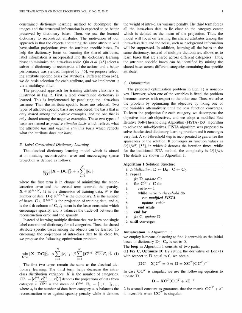
Fig. 1. Overview of the Framework. The label constrained dictionarylearning module forces the dictionary to focus on learning the shared attributespecific bases by penalizing the intra-class variance. Then the mutilayer filterhelps discover the representative and robust bases for each attribute.

attributes and discriminative attributes. The semantic attributeshave semantic meanings assigned to them while discriminativeattributes do not have exact semantic meanings.

Attributes are used to describe the characteristics and qualityof an object or scene, such as materials, appearances, andfunctions. Attributes can provide a more detailed descriptionof an image [2], [3] and can make key-word based imagesearch feasible (e.g., young asian men with glasses). Besides,attributes are also composable, they can be combined fordifferent specificities, i.e., a consumer might want to find high-heeled shiny shoes. The most important property of attributes,such as color and shape, is that they can be transferred amongdifferent object categories. Zero-shot learning [4] is proposedbased on this property. First, attribute classifiers are pre-learned from their related objects. Then the target object can berecognized based on its binary attribute representation, whichrequires no training examples. The attribute representationis a binary vector whose elements are either one or zero,indicating the presence or absence of a specific attribute [5].The binary attributes can efficiently split the image space [6].k binary attributes can split images into 2k space. In addi-tion, abnormality prediction can be achieved [7] by checkingthe absence of typical attributes or the presence of atypicalattributes. However, the binary classifiers for attributes fail in


capturing the relative strength of attributes between images.In order to capture more generative semantic relationships,relative attributes were introduced by Parikh and Grauman [8].A ranking function is learned for each attribute whose outputis a continuous score denoting the strength of attributes in animage. With the help of relative attributes, we can describeimages relative to other images by comparing their attributescores. A more recent study showed that the performance ofrelative attribute ranking functions can be improved by usinglocal parts that are shared through categories instead of usingglobal features [9], [10].

In most situations, attributes are predefined with semanticmeanings. Attribute vocabulary can be manually designed,such as the ‘Animal with Attributes’ dataset [11] where 85binary attributes about 50 animal classes are defined. How-ever, human defined attributes might be insufficient and notdiscriminative, especially for the categories which are not wellstudied by linguists. To tackle this problem, Parikh et al. [12]proposed augmenting the vocabulary actively to ensure that thenew attributes can be inter-class discriminative. The rich webdata can also be utilized to mine attributes, which requires nohuman annotators. Berg et al. [13] proposed mining attributevocabulary automatically from web images and noisy textdescriptions. They also demonstrated that some attributes canbe localized, i.e., attributes can be characterized into localor global ones. As the localized attributes can provide fine-grained information, they are more discriminative when theobject categories are quite close to each other (e.g. birdspecies recognition). A local attribute discovery model wasintroduced by Duan et al. [14] to determine a local attributevocabulary. In most situations, attributes are defined prior tolearning their corresponding statistical models. We can alsolearn the models first, and then decide whether to assignsemantic meanings to the learned models. For example, somediscriminative attributes [5] without semantic meanings areproposed for object recognition. Thus, attributes do not haveto be associated with semantic meanings.

Current attribute learning methods usually map the low-level features directly to attributes. The dimension of low-levelfeature vector is usually very high because of the concatenationof various features, such as SIFT, Color SIFT and HOG.Jayaraman et al. [15] pointed out that the performance ofattribute classifiers could be improved through feature se-lection because of the intrinsic mappings between attributesand features. Take color attributes (red, green, yellow, etc.)for example, the color attributes can be better trained onthe dimensions corresponding to color histogram bins, wherestexture attributes (furry, silky, etc.) prefer texture features.

Most works perform feature selection by adding differ-ent regularizers into the loss function to encourage sparsityselection of features, and the correlation between attributesis considered simultaneously [5], [16], [15]. For instance,l1-norm encourages feature competition among groups, l2-norm encourages feature sharing among groups, and l2,1-norm encourages intra-group feature sharing and inter-groupcompetition. Regardless of regularizer types, the underlyingintuition remains the same, i.e., encourage the semanticallyclose attributes to share similar feature dimensions. The se-

mantic correlation is either measured according to the semanticdistance mined from the web, e.g., using WordNet [17], orfrom attributes’ co-occurrence probability as proposed by Hanet al. [16]. However, it is hard to judge to what extent thevisual appearance similarity can be reflected by semanticcloseness, and there is no guarantee that the semanticallyclose attributes are visually similar. For example, the semanticdistance between orange and apple is 2.25 and 0.69 betweenorange and mandarin, which are calculated based on theLeacock-Chodorow similarity measurement from WordNet[17]. However, we could not say that orange is visually moresimilar to apple than mandarin. In fact, orange should bemore visually similar to mandarin as they have the sameshape and color. Furthermore, the raw features might be verynoisy and feature selection [18] over the raw features discardsthe structure information as each feature dimension is treatedindependently.

To address this issue, we propose a novel framework whichconsists of a label constrained dictionary learning module anda multilayer filter to perform basis selection. Fig.1 shows theoverview of the introduced framework. Different from theconventional methods which perform feature selection overthe raw features, we adopt a multilayer filter to do featureselection at the dictionary level, as a dictionary is expected tocapture the higher-level structure of images [19]. First, a labelconstrained dictionary is constructed by suppressing the intra-class training data. Second, we design a multilayer filter toperform basis selection for each attribute independently. Thebasis is regarded as attribute specific basis if only the positiveor only the negative examples have large and stable distributionover it. The larger the distribution is, the more representativethe basis is. The smaller the standard deviation is, the morerobust the basis is. Therefore, in the multilayer filter, two filtersare designed for attribute specific bases selection, namely,µ-Filter and σ-Filter. The µ-Filter selects the representativebases, and the σ-Filter select the robust bases from the repre-sentative bases. Common bases are marked if both the positiveand negative examples have large distribution over them. Thecommon bases are only used for the reconstruction while theattribute specific bases are used both for image reconstructionand attribute classifier learning. Finally, the attributes of animage are predicted by a set of linear SVM classifiers withits projection over the attribute specific bases. To sum up, thispaper makes the following contributions:• A novel label constrained dictionary learning method is

proposed which suppresses intra-class noise and encouragesthe projections of intra-class training data to lie close by.

• A multilayer filter is designed for dictionary basis selection.Two filters, namely µ-Filter and σ-Filter are designed toselect the robust and representative bases for each attribute.This paper is organized as follows. Section 2 reviews related

work. Section 3 introduces our proposed framework. Experi-ments are described in Section 4, while Section 5 concludesthis paper.

II. RELATED WORK

In this section, we review the related work on attributelearning, feature selection and dictionary learning.


=

…{ {

… … …

…

……

…=

…

Distribution

…

…

…

…

…

SelectedBasis Distributions

…

Positive Samples

Negative Samples

…

…

…

…

…

…

…Linear Classifier

furry (√) big (√) white (√)bush (x)�blue (x)

fox hamster

…

horse

……

Different Categories

1 2 3 4 5 6 7 8 9 100

1

2

3

4

5

6

7

1 2 3 4 5 6 7 8 9 100

1

2

3

4

5

6

7

1 2 3 4 5 6 7 8 9 100

1

2

3

4

5

6

7

Category-Attribute Matrix Informative Dictionary Learning

Basis Selection for Each Attribute

Positive Samples: σ ×10-36 6.5 7 7.5 8 8.5 9 9.5 10 10.5

Neg

ativ

e Sa

mpl

es: σ

×10-3

6

6.5

7

7.5

8

8.5

9

9.5Attr BasisNosie

Positive Samples: µ ×10-40 2 4 6 8 10 12 14 16 18

Neg

ativ

e Sa

mpl

es: µ

×10-4

2

4

6

8

10

12

14Common BasisAttr BasisNosie

Attribute Detection

X

fox : X(1)

D C(1) C(S)

d1, d3, d5

Hidden AttributeSpecific Bases

C(1)

C(S)µ1,�1

µ2,�2

µ3,�3

µ4,�4

µ5,�5

µ1,�1

µ2,�2

µ3,�3

µ4,�4

µ5,�5

D C(1) C(S)

x D c

µ Filter

� Filter

BoW Feature

horse : X(S)

Fig. 2. Pipeline Overview. (top) A label constrained dictionary is learned by encouraging intra-class samples lie close by. (bottom left) Multilayer filter:µ-Filter & σ-Filter are designed to select a set of robust and representative attribute specific bases to reconstruct each attribute. (bottom right) Attributes arepredicted by linear SVM classifiers using the distributions over the attribute specific bases.

A. Attribute Learning

Attributes are middle level features which are sharedthrough categories. Human naturally describe visual conceptswith attributes. For instance, when we describe a person, wemight say that he is a male, has short hair, and wear jeans. Wealso recognize objects or scenes through their attributes. Forexample, zebra has stripes. Recent studies revealed that thehigh performance of convolutional networks is ascribed to theattribute centric nodes within the net [20], and weakly super-vised convolutional neural networks works well for attributedetection [10]. Besides, attributes usually provide more detailsof an image. In some situations, people may be interested notonly in the object categories (e.g., cat, dog, bike), but also inthe detailed information (e.g., is silky, has legs, is cute) of animage. In order to describe images with detailed information,Farhadi et al. [21] proposed describing an image based onsemantic triples <object, action, scene>. The semantic triplelinks an image to a descriptive sentence. However, the methodin [21] heavily relies on the object and scene classifiers togenerate triples. Han et al. [22] proposed a hierarchical tree-structured semantic unit to describe an image at differentsemantic levels (attribute level, category level, etc). Thus, evenif the object or scene classifier is unavailable, some attributelevel information could still be provided.

As attributes are shared through categories, they also havegreat potential in object recognition tasks [23], [1], [24].Latent attributes are utilized to improve the performance of

object classifiers by taking the object-attribute relationship intoconsideration [25], [26]. Wang et al. [27] took a further stepto improve object classification performance by employingthe attribute-attribute relationship. Besides, attributes can helprecognize object when no training data is available. Lampertet al. [4] proposed zero-shot learning to predict unseen objectsbased on its binary attribute representation. Parikh et al. [8]improved the performance of zero-shot learning by utilizingrelative attributes. Relative attributes can also be used tobenefit interactive image search [28]. Based on the relativeranking scores, the system is enabled to adjust the strengthof attributes to meet users’ preferences. For active learning,attributes can propagate the impact of annotations through theentire model. Relative attributes can accelerate discriminativelearning with few examples [29], [30], [31] as the mistakelearned from one image can be transferred to many otherimages. For example, when the learner considers an imageto be too open to be a forest, all other images more openthan the current one will be filtered out. Attributes are alsosuccessfully applied into action recognition [32], [33], [34] andevent detection [35]. Since attributes have wide applications,the performance of attribute classifiers are crucial.

B. Feature Selection for Attributes

There exist many different attribute groups, such as person-related attributes (e.g., is male, has hat, has glasses), sceneattributes (e.g., trees, clouds, leaves) and animal attributes.


In animal attributes group, there are also subgroups, suchas textures (e.g., stripes, furry, spots), part-of-body (horns,claws, tusks) and colors (black, white, blue). Jayaraman etal. [15] pointed out that the attribute classifiers would havedifferent performances when different types of features wereused because of the intrinsic relations between attributes andfeature types.

The conventional methods learn attribute classifiers by map-ping all the low-level raw features directly to each semanticattribute independently. However, many attributes are stronglycorrelated through the object categories. For example, mostobjects that have wheels are made of metal. Then when we tryto learn has wheel, we may accidentally learn made of metal.To solve the correlation problem, various feature selectiontechniques are developed, most of which are implemented byintegrating regularizers into the loss function. The underlyingintuition behind feature selection is that only a portion offeature dimensions defines an attribute.

Thus, feature selection is an important process to improvethe performance of attribute classifiers. Many works imple-ment feature selection directly on the low-level raw featuresby using different regularizers, such as l1-norm combined withl2-norm, l2,1-norm [15], [36], or l2,p-norm, to encourage intra-group feature sharing and inter-group feature competition, aswell as different loss functions, such as linear regression orlogistic regression. Most regularizers are employed to get ridof the influence of attribute correlations. However, most cur-rent works revealed that the performance of attribute classifierscould be improved by harnessing attribute correlations ratherthan removing it [37], [38]. Han et al. [16] measured theattribute correlation through their co-occurrence probabilityamong the object categories. A symmetric connected graphis constructed to represent the correlation between each pairof attributes, and the weights of the edges denote the quan-tified correlations. Then the correlation is put into l1-normregularizer. The relation between attributes does not have tobe symmetric. For instance, the presence of necktie stronglyindicates the presence of collar while the presence of collardoes not indicate the presence of necktie. An asymmetricattribute correlation was defined in [39]. Usually, attributecorrelation is regarded as an indicator of the feature sharingextent between attributes, and it is used to encourage featuresharing while feature competition is neglected. Regardless ofthe regularizer types, all these methods rely on regularizers toperform feature selection.

C. Dictionary Learning

Dictionary learning (or sparse coding) has been originallydeveloped in order to explain the early visual processing in thebrain [40]. An over-complete dictionary is built by minimizingthe reconstruction error of the training samples where thelearned bases are edges. Thus a more succinct and compactrepresentation of an image can be obtained by its approximatedecomposition over the dictionary bases. Based on sparsecoding, hierarchical deep belief net model was proposed [41].While learned bases in the first layer correspond to edges,the learned bases in the second layer correspond to object

components which are the combinations of edges. Whenmultiple objects are used for training, the learned bases arethe features shared across object classes. With the help ofdictionary learning, the unlabeled data can be utilized to helpsupervised learning tasks, as usually the labeled data is verytime-consuming to obtain. Dictionary learning allows us to usea small labeled training set to do a much better job at trainingclassifiers [19].

More recently, dictionary learning has been applied to solveevent detection [42], [43] and action detection problems [44].Actions in videos are often atomic and largely defined by bodyposes, while events are composite and defined by objects andscenes. Qiu et al. [45] proposed learning a compact dictionaryfor actions, in which each basis is treated as an action attribute.In addition, dictionary learning can also be applied to imageclustering tasks. Ramirez et al. [46] proposed learning multipledictionaries for multiple categories to better embed the classinformation. The new data are assigned to the cluster whosedictionary can minimize the reconstruction error. Many dif-ferent dictionary learning variants are studied by researchers,such as pairwise dictionary learning [47]. Another variant ofdictionary learning was considered in [48] by integrating themanifold information and dictionary learning into the sameframework.

Some work tried to bridge attributes and dictionary learning.Feng et al. [5] proposed an adaptive dictionary learningmethod for object recognition. Each image is reconstructed bya linear binary combination of dictionary bases, and each basisis regarded as one attribute. However, these attributes haveno semantic meanings, and they can hardly be generalizedto novel categories. Besides, the dictionary is usually trainedby unlabeled data [46], [19] and a lot of noise bases thatcome from other unrelated objects are also learned. Whenlabeled data are available, a label constrained dictionary canbe learned, which is expected to encourage the sparse rep-resentation of intra-class data lie close by. In our work, thisis implemented by a special regularizer and a modified FastIterative Soft-Thresholding Algorithm (FISTA) is adopted tosolve the problem.

III. LABEL CONSTRAINED DICTIONARY LEARNING ANDATTRIBUTE SPECIFIC BASIS SELECTION

In this section, we further discuss the underlying motivationof the proposed framework and present an overview of ourapproach. Then, our label constrained dictionary learningmethod is introduced. Finally, we elaborate the multilayer filterfor basis selection.

A. Motivation and Overview

Most works employ feature selection to improve the per-formance of attribute classifiers. The underlying assumptionis that an attribute is defined by a certain amount of featuredimensions. Thus, attributes are often learned jointly in amulti-task learning framework [49], [50], [51], [52] in orderto encourage feature sharing among correlated attributes.

However, feature selection discards the structural infor-mation of an image. Inspired by [5], we propose a label


constrained dictionary learning method to decompose theimages and the structural information is expected to be betterpreserved by dictionary bases. Then, we use the learneddictionary to reconstruct attributes. The motivation of ourapproach is that the objects containing the same attribute willhave similar projections over the attribute specific bases. Tohelp the dictionary focus on learning the shared attributes,label information is incorporated into the dictionary learningphase to minimize the intra-class noise. Qiu et al. [45] select asubset of dictionary to reconstruct all the actions and a betterperformance was yielded. Inspired by [45], we propose select-ing attribute specific bases for attributes. Different from [45],we do basis selection for each attribute, and we implement itvia a multilayer filter.

The proposed approach for training attribute classifiers isillustrated in Fig. 2. First, a label constrained dictionary islearned. This is implemented by penalizing the intra-classvariance. Then the attribute specific bases are selected. Twotypes of attribute specific basis are considered: the basis that isonly shared among the positive examples, and the one that isonly shared among the negative examples. These two types ofbasis are named as positive stimulus basis which reflects whatthe attribute has and negative stimulus basis which reflectswhat the attribute does not have.

B. Label Constrained Dictionary Learning

The classical dictionary learning model which is aimedat minimizing reconstruction error and encouraging sparseprojection is defined as follows:

minD,C‖X−DC‖2F + λ

N∑i=1

‖ci‖1

where the first term is in charge of minimizing the recon-struction error and the second term controls the sparsity.X ∈ RM×N , M is the dimension of training data, N is thenumber of data, D ∈ RM×L is the dictionary, L is the numberof bases, C ∈ RL×N is the projection of training data, and ciis the i-th column of C, l1-norm is the lasso constraint whichencourages sparsity, and λ balances the trade-off between thereconstruction error and the sparsity.

Instead of learning multiple dictionaries, we learn one singlelabel constrained dictionary for all categories. Thus, the sharedattribute specific bases among the objects can be learned. Toencourage the projections of intra-class data to lie close by,we propose the following optimization problem:

minD,C‖X−DC‖2F+α

N∑i=1

‖ci‖1+βK∑s=1

‖C(s)−C(s)Es‖2F (1)

The first two terms remain the same as the classical dic-tionary learning. The third term helps decrease the intra-class distribution variances. K is the number of categories.C(s) = [c

(s)1 , c

(s)2 , ..., c

(s)st ] denotes the projections of data from

category s. C(s) is the mean of C(s). Es = [1, 1, ...]1×st ,where st is the number of data from category s. α balances thereconstruction error against sparsity penalty while β denotes

the weight of intra-class variance penalty. The third term forcesall the intra-class data to lie close to the category centerwhich is defined as the mean of the projection. Thus, themodel will focus on learning the shared attributes among theintra-class data and the noise, such as background informationwill be suppressed. In addition, learning all the bases in thesame dictionary, instead of multiple dictionaries, allows us tolearn bases that are shared across different categories. Thus,the attribute specific bases can be identified by mining theshared bases across different categories containing that specificattribute.

C. Optimization

The proposed optimization problem in Eqn.(1) is noncon-vex. However, when one of the variables is fixed, the problembecomes convex with respect to the other one. Thus, we solvethe problem by optimizing the objective by fixing one ofthe variables alternatively until the loss function converges.To learn the projection for each category, we decompose theobjective into sub-objectives, and we adopt a modified FastIterative Soft-Thresholding Algorithm (FISTA) [53] algorithmto solve the sub-objectives. FISTA algorithm was proposed tosolve the classical dictionary learning problem and it convergesvery fast. A soft-threshold step is incorporated to guarantee thesparseness of the solution. It converges in function values asO(1/k2) [53], in which k denotes the iteration times, whilefor the traditional ISTA method, the complexity is O(1/k).The details are shown in Algorithm 1.

Algorithm 1 Solution Structure1: Initialization: D← D0 , C← C0

2: repeat3: fix D, update C:4: for C(s) ∈ C do5: ratio← 16: while ratio > threshold do7: run modified FISTA8: update ratio9: end while

10: end for11: fix C, update D12: until converges

Initialization in Algorithm 1:we employ k-means clustering to find k centroids as the initialbases in dictionary D0. C0 is set to 0.The loop in Algorithm 1 consists of two parts:(1) Fix C, Optimize D: By setting the derivative of Eqn.(1)with respect to D equal to 0, we obtain,

(DC−X)CT = 0⇒ D = XCT (CCT )−1

In case CCT is singular, we use the following equation toupdate D.

D = XCT (CCT + λI)−1

λ is a small constant to guarantee that the matrix CCT + λIis invertible when CCT is singular.


(2) Fix D, Optimize C: To update C, we decompose theobjective into a set of sub-objectives. Each sub-objectivecorresponds to one category.

Note that when D is fixed, L(D;C(s);X(s)) is independentfrom each other with respect to s. Then the objective Eqn.(1)can be written as:

minC

K∑s=1

L(D;C(s);X(s)) =

K∑s=1

minC(s)

L(D;C(s);X(s))

Thus the original objective function is decomposed into aset of sub-objective functions with respect to each category.The third term in Eqn.(1) makes the ci and cj within thesame category become dependent on each other. Thus, ci andcj must be updated simultaneously in order to make the wholesystem converge. We modify the FISTA algorithm to tackle theproblem. The new sub-objective in our model is as follows,

F=∑

c∈C(s)

‖Dc− x‖2 + α‖c‖1 + β‖c− 1

N

∑ck∈C(s)

ck‖2

From the equation above, we can find that, for training datax ∈ X(s), its distribution c (c ∈ C(s)) depends on other ck(ck ∈ C(s)). Thus, the sub-objectives cannot be optimizedindependently. We modify the FISTA algorithm to optimizethe sub-objectives from the same group simultaneously. Thesub-objectives are grouped together if the training data belongto the same group. Then when updating C(s), all cj ∈ C(s)

are updated simultaneously for j = 1, ..., st.

cj := cj − γ∂F

∂cj

Please refer to [53] for the details about how to select the ap-propriate γ, as well as the following soft thresholding processto delete the small values in cj. This updating procedure ofC(s) continues until convergence. To judge whether all the cjin the same category converge or not, we refer to the metricratio, which is defined as:

ratio = mincj∈C(s)

‖cj − cj‖2/‖cj‖2

in which cj denotes the updated value of cj. The thresh-old controls the number of iterations of each category. Ifratio < threshold, the update procedure for the category willbe terminated. We run the same procedure for each category.In Algorithm 1, line 4 to line 10 represent the pseudo-code toupdate C. The setting of the values is available at the end ofsection 4.3.2. The convergence condition required in step 12of the algorithm is similar to the ratio defined in the FISTAalgorithm.

D. Multilayer Filter - Basis Selection

After learning the label constrained dictionary, we rely onthe statistics of the projection C to divide the bases into 3groups, the common bases, attribute specific bases, andnoise bases. Common Bases are the bases over which boththe positive and negative examples have large and stabledistributions. Attribute Specific Bases are the bases over whichonly the positive or only the negative samples have large andstable distributions. Noise Bases are the remained ones.

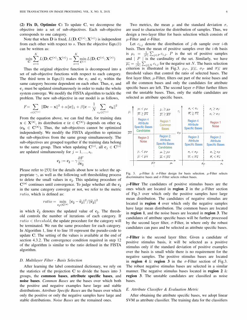
Two metrics, the mean µ and the standard deviation σ,are used to characterize the distribution of samples. Thus, wedesign a two-layer filter for basis selection which consists ofµ-Filter and σ-Filter.

Let ci,j denote the distribution of j-th sample over i-thbasis. Then the mean of positive samples over the i-th basisis µi = 1

|P |∑

j∈P ci,j . P is the set of positive samplesand | P | is the cardinality of the set. Similarly, we haveµi =

1|N |

∑j∈N ci,j for the negative set N . The basis selection

criterion is illustrated in Fig.3. µP , µN , σP and σN arethreshold values that control the ratio of selected bases. Thefirst layer filter, µ-Filter, filters out part of the noise bases andall the common bases and only the candidates for attributespecific bases are left. The second layer σ-Filter further filtersout the unstable bases. Thus, only the stable candidates areselected as attribute specific bases.

Region 1Common

Bases

Region 3Noise

Region 2:Attribute

Specific BasesCandidates

Region 4Attribute

Specific BasesCandidates

Region 2Attribute

Specific Bases

Region 4Attribute

Specific Bases

Region 3Attribute

Specific Bases

Region 1Noise

Fig. 3. µ-Filter & σ-Filter design for basis selection. µ-Filter selectsdiscriminative bases and σ-Filter selects robust bases.

µ-Filter The candidates of positive stimulus bases are theones which are located in region 2 in the µ-Filter sectionof Fig.3 over which only the positive samples have largemean distribution. The candidates of negative stimulus arelocated in region 4 over which only the negative sampleshave large mean distribution. The common bases are locatedin region 1, and the noise bases are located in region 3. Thecandidates of attribute specific bases will be further processedby the second layer filter, σ-Filter, in where only the robustcandidates can pass and be selected as attribute specific bases.

σ-Filter is the second layer filter. Given a candidate ofpositive stimulus basis, it will be selected as a positivestimulus only if the standard deviation of positive examplesover the basis is small while there is no requirement for thenegative samples. The positive stimulus bases are locatedin region 4 & region 3 in the σ-Filter section of Fig.3.The robust negative stimulus bases are selected in a similarmanner. The negative stimulus bases located in region 2 &region 3. The unstable candidates are classified as noisebases.

E. Attribute Classifier & Evaluation MetricAfter obtaining the attribute specific bases, we adopt linear

SVM as attribute classifier. The training data for the classifiers


arch jewellery shop water tower palace

… … … …

buffalo chimpanzeehorse rabbit

… … … …

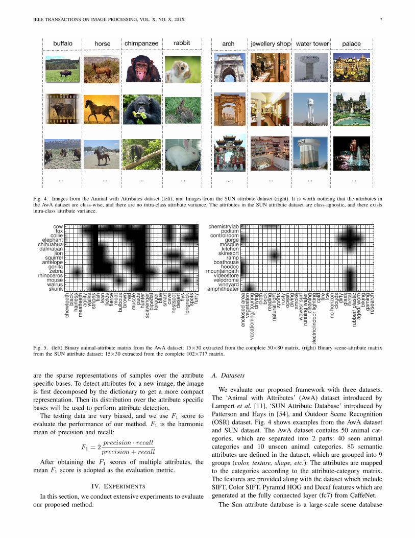
Fig. 4. Images from the Animal with Attributes dataset (left), and Images from the SUN attribute dataset (right). It is worth noticing that the attributes inthe AwA dataset are class-wise, and there are no intra-class attribute variance. The attributes in the SUN attribute dataset are class-agnostic, and there existsintra-class attribute variance.

en

clo

sed

are

ave

ge

tatio

nva

catio

nin

g/

tou

rin

gd

rivi

ng

clo

thb

rick

rea

din

gn

atu

ral l

igh

tsp

ort

sru

sty

oce

an

div

ing

smo

kew

ave

s/ s

urf

run

nin

g w

ate

rcl

ea

nin

ge

lect

ric/

ind

oo

r lig

htin

gco

ldfir

eic

en

o h

orizo

ncl

ou

ds

dirty

gla

ssm

eta

lru

bb

er/

pla

stic

ag

ed

/ w

orn

bik

ing

ga

min

gre

sea

rch

chemistrylabpodium

controlroomgorge

mosquekitchen

skiresortramp

boathousehoodoo

mountainpathvideostorevelodrome

vineyardamphitheater

che

wte

eth

bla

ckh

airle

ssm

ea

tte

eth

ag

ility

wa

lks

strip

es

fish

lea

nfie

lds

fierc

em

ea

tb

ulb

ou

sb

row

nre

dm

usc

lep

ad

sh

un

ter

sca

ven

ge

rb

ipe

da

lfo

rag

er

blu

esm

art

cave

ne

stsp

ot

de

sert

flys

lon

gn

eck

spo

tsfu

rry

cowfox

collieelephant

chihuahuadalmatian

lionsquirrel

antelopegorillazebra

rhinocerosmousewalrusskunk

Fig. 5. (left) Binary animal-attribute matrix from the AwA dataset: 15×30 extracted from the complete 50×80 matrix. (right) Binary scene-attribute matrixfrom the SUN attribute dataset: 15×30 extracted from the complete 102×717 matrix.

are the sparse representations of samples over the attributespecific bases. To detect attributes for a new image, the imageis first decomposed by the dictionary to get a more compactrepresentation. Then its distribution over the attribute specificbases will be used to perform attribute detection.

The testing data are very biased, and we use F1 score toevaluate the performance of our method. F1 is the harmonicmean of precision and recall:

F1 = 2precision · recallprecision+ recall

After obtaining the F1 scores of multiple attributes, themean F1 score is adopted as the evaluation metric.

IV. EXPERIMENTS

In this section, we conduct extensive experiments to evaluateour proposed method.

A. Datasets

We evaluate our proposed framework with three datasets.The ‘Animal with Attributes’ (AwA) dataset introduced byLampert et al. [11], ‘SUN Attribute Database’ introduced byPatterson and Hays in [54], and Outdoor Scene Recognition(OSR) dataset. Fig. 4 shows examples from the AwA datasetand SUN dataset. The AwA dataset contains 50 animal cat-egories, which are separated into 2 parts: 40 seen animalcategories and 10 unseen animal categories. 85 semanticattributes are defined in the dataset, which are grouped into 9groups (color, texture, shape, etc.). The attributes are mappedto the categories according to the attribute-category matrix.The features are provided along with the dataset which includeSIFT, Color SIFT, Pyramid HOG and Decaf features which aregenerated at the fully connected layer (fc7) from CaffeNet.

The Sun attribute database is a large-scale scene database


Raw DL LC_DL BS+LC_DL

Mean F1 Score

0.00

0.05

0.10

0.15

0.20

0.25

0.30

0.35

0.40

0.45

0.50 AwA Dataset (decaf)

Raw DL LC_DL BS+LC_DL

Mean F1 Score

0.30

0.35

0.40

0.45

0.50

0.55

0.60

0.65

0.70

0.75

0.80 SUN Dataset (GIST)

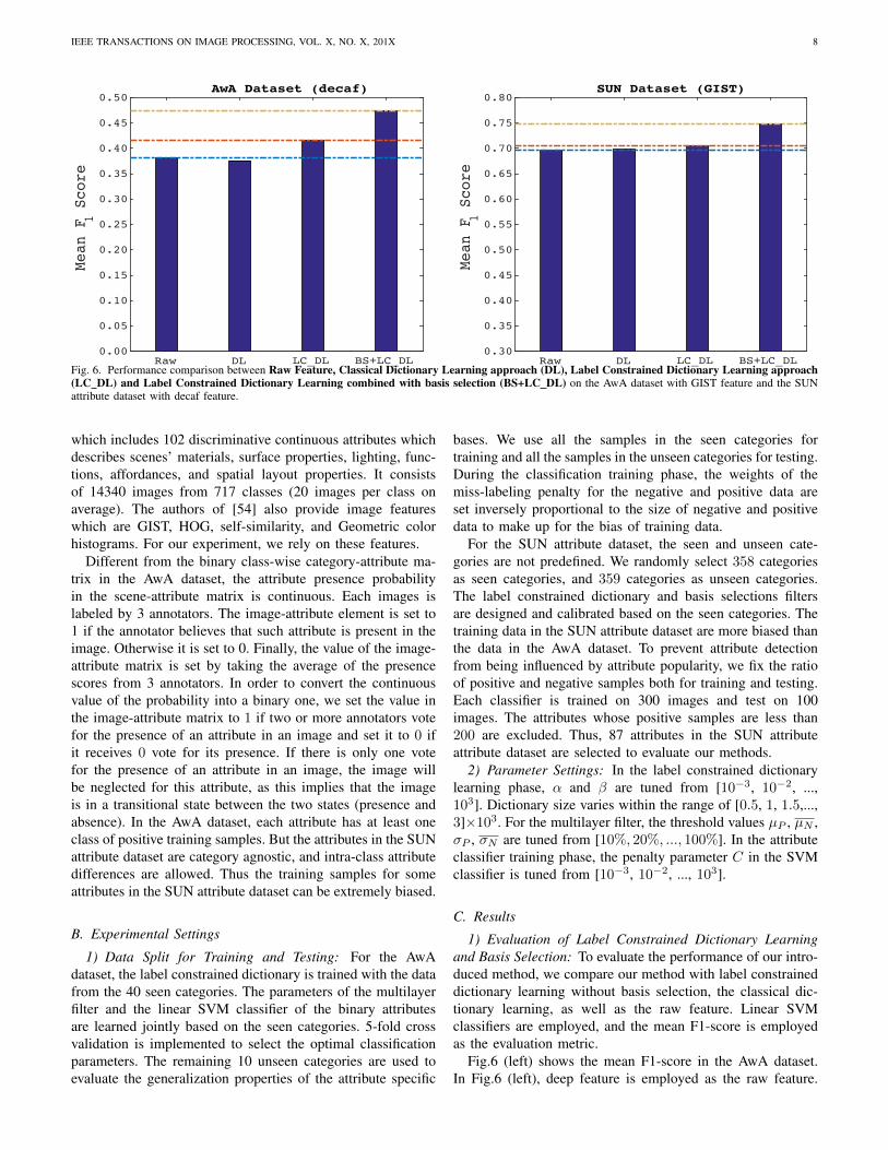
Fig. 6. Performance comparison between Raw Feature, Classical Dictionary Learning approach (DL), Label Constrained Dictionary Learning approach(LC DL) and Label Constrained Dictionary Learning combined with basis selection (BS+LC DL) on the AwA dataset with GIST feature and the SUNattribute dataset with decaf feature.

which includes 102 discriminative continuous attributes whichdescribes scenes’ materials, surface properties, lighting, func-tions, affordances, and spatial layout properties. It consistsof 14340 images from 717 classes (20 images per class onaverage). The authors of [54] also provide image featureswhich are GIST, HOG, self-similarity, and Geometric colorhistograms. For our experiment, we rely on these features.

Different from the binary class-wise category-attribute ma-trix in the AwA dataset, the attribute presence probabilityin the scene-attribute matrix is continuous. Each images islabeled by 3 annotators. The image-attribute element is set to1 if the annotator believes that such attribute is present in theimage. Otherwise it is set to 0. Finally, the value of the image-attribute matrix is set by taking the average of the presencescores from 3 annotators. In order to convert the continuousvalue of the probability into a binary one, we set the value inthe image-attribute matrix to 1 if two or more annotators votefor the presence of an attribute in an image and set it to 0 ifit receives 0 vote for its presence. If there is only one votefor the presence of an attribute in an image, the image willbe neglected for this attribute, as this implies that the imageis in a transitional state between the two states (presence andabsence). In the AwA dataset, each attribute has at least oneclass of positive training samples. But the attributes in the SUNattribute dataset are category agnostic, and intra-class attributedifferences are allowed. Thus the training samples for someattributes in the SUN attribute dataset can be extremely biased.

B. Experimental Settings

1) Data Split for Training and Testing: For the AwAdataset, the label constrained dictionary is trained with the datafrom the 40 seen categories. The parameters of the multilayerfilter and the linear SVM classifier of the binary attributesare learned jointly based on the seen categories. 5-fold crossvalidation is implemented to select the optimal classificationparameters. The remaining 10 unseen categories are used toevaluate the generalization properties of the attribute specific

bases. We use all the samples in the seen categories fortraining and all the samples in the unseen categories for testing.During the classification training phase, the weights of themiss-labeling penalty for the negative and positive data areset inversely proportional to the size of negative and positivedata to make up for the bias of training data.

For the SUN attribute dataset, the seen and unseen cate-gories are not predefined. We randomly select 358 categoriesas seen categories, and 359 categories as unseen categories.The label constrained dictionary and basis selections filtersare designed and calibrated based on the seen categories. Thetraining data in the SUN attribute dataset are more biased thanthe data in the AwA dataset. To prevent attribute detectionfrom being influenced by attribute popularity, we fix the ratioof positive and negative samples both for training and testing.Each classifier is trained on 300 images and test on 100images. The attributes whose positive samples are less than200 are excluded. Thus, 87 attributes in the SUN attributeattribute dataset are selected to evaluate our methods.

2) Parameter Settings: In the label constrained dictionarylearning phase, α and β are tuned from [10−3, 10−2, ...,103]. Dictionary size varies within the range of [0.5, 1, 1.5,...,3]×103. For the multilayer filter, the threshold values µP , µN ,σP , σN are tuned from [10%, 20%, ..., 100%]. In the attributeclassifier training phase, the penalty parameter C in the SVMclassifier is tuned from [10−3, 10−2, ..., 103].

C. Results

1) Evaluation of Label Constrained Dictionary Learningand Basis Selection: To evaluate the performance of our intro-duced method, we compare our method with label constraineddictionary learning without basis selection, the classical dic-tionary learning, as well as the raw feature. Linear SVMclassifiers are employed, and the mean F1-score is employedas the evaluation metric.

Fig.6 (left) shows the mean F1-score in the AwA dataset.In Fig.6 (left), deep feature is employed as the raw feature.


Similarly, Fig.6 (right) shows the mean F1-score in the SUNattribute dataset where the GIST [55] feature is employed.

From Fig.6 we can observe that our method outperformsall the baselines for both datasets. The classical dictionarylearning has similar performance with the raw feature. Thelabel constrained dictionary learning outperforms both the rawfeature and classical dictionary learning method. For the AwAdataset, the label constrained dictionary learning outperformsthe raw feature by 3.5%. However, for the SUN attributedataset, the improvement is very small (0.9%). There is nosurprise that the label constrained dictionary learning has amore remarkable effect on the AwA dataset compared withthe SUN attribute dataset. This is because the attributes inthe AwA dataset are class-wise. Then, there is no intra-classattribute variance. However, for the SUN attribute dataset,the attribute is class agnostic. Then, there exists a certainamount of intra-class attribute variance. Our label constraineddictionary learning is aimed at suppressing the intra-classnoise. Consequently, the performance of the label constraineddictionary learning is restricted by the intra-class attributevariance. The reason why the label constrained dictionarylearning still outperforms the raw feature in the SUN attributedataset is that most images within the same class still share thesame attributes. Thus, the label constrained dictionary learningcan still help focus on learning those attributes which areshared through the whole class.

We can also observe that basis selection further improvesthe performance of label constrained dictionary learning by7.89% on the AwA dataset, and 4.4% on the SUN dataset.

2) Multilayer Filter Parameter Settings and ConvergenceStudy: We employ the AwA dataset to study the sensitivity ofthe multilayer filter parameters. Fig.7 shows the grid plot ofthe mean F1 score with respect to different filter parameters.The dictionary size is set to be 2000. The µ-Filter and σ-Filtercontrol the ratio of selected bases. The ratio of the selectedbases ranges from 10% to 100%. The performance is measuredon the unseen object categories. The value of the bar is themean F1 score of all the 85 attributes. From Fig.7, we observethat when more bases are selected either by the µ-Filter orby the σ-Filter, the mean F1 score tends to decrease. Themaximum F1 score is obtained when both the µ-Filter and theσ-Filter only select 10% bases. From this observation, we canconclude that, the basis selection improves the performance ofattribute detectors, and the best ratio of the basis selection liesclose to 10% which could be mined out by doing a fine-grainedsearch of the ratio. The optimal filter parameter settings forthe SUN attribute dataset are configured in the same way. Asthe training samples in the SUN attribute dataset is relativelysmall compared with that in the AwA dataset, its dictionarysize is set to be 500.

Fig.8 illustrates the first layer filter, namely, the µ-Filter.The two decision boundaries control the ratio of the selectedcandidates of the attribute specific bases before putting theminto σ-Filter. The decision boundaries in the µ-Filter aredetermined by two threshold values, µP , µN which correspondto the mean of the distribution of the positive samples,and to the mean of the distribution of the negative samplesrespectively. The two boundaries divide the bases into four

1 0.9

0.80.7

0.6

σ

0.50.4

0.30.2

0.10.9

0.80.7

0.60.5

µ

0.40.3

0.20.1

0.38

0.39

0.4

0.41

0.42

0.43

0.44

0.45

F1 s

core

Fig. 7. Mean F1 Score of 85 attributes for the AwA dataset over different µ& σ settings

Fig. 8. Scatter Plot of bases over positive and negative samples in µ-Filter(20% bases are selected).

regions. However, only the bases in the upper-left region andthe lower-right region are selected as representative bases. Thebases in the upper-left region represent what the attribute doesnot have. The bases in the lower-right region represent whatthe attribute has. The bases in lower-left region are regardedas noise as both positive and negative samples have smalldistributions over them. By setting the boundaries to differentvalues, different amount of bases can be selected.

For µ filter, we sort the bases in ascending order with respectto µ and µ separately. Then we select the desired amount ofpercentage (10%, 20%, etc) with respect to µ and µ separately.The attribute specific bases are then selected from these basesby removing their overlap (noisy bases).

Fig.9 is the scatter plot of basis selection with the σ-Filter.After the selection of representative bases, the σ-Filter is ap-plied to discover the candidates which are robust enough to beattribute specific bases. The decision boundaries in the σ-Filterare determined by two threshold values, σP and σN whichcorrespond to the standard deviation of positive samples, andthe standard deviation of negative samples respectively. Ifeither the positive samples or the negative samples have large


Fig. 9. Scatter Plot of bases over positive and negative samples in σ-Filter(20% bases are selected).

mean and small standard deviations over the representativebases, the bases will be selected as attribute specific bases.Otherwise, they will be filtered out. Thus, the robust andrepresentative attribute specific bases are obtained.

We also study the convergence of our algorithm with theAwA dataset. We rely on K-means to select K most repre-sentative basis to initialize the dictionary. Fig.10 (a) showsthe convergence curve of the overall function. The thresholdcontrols the number of iterations of the algorithm for eachcategory. We set the threshold to 0.01. Fig.10 (b) shows thelog plot of the loss when updating C(s) for five categories. Itshows that all the five sub-objectives converge very fast. Thethreshold could be adjusted to a smaller number if we expectthe algorithm to have more iterations.

Iteration (a)50 100 150 200 250 300 350 400 450

Ove

rall

Obj

ectiv

e Va

lue

×105

2

3

4

5

6

7

8

9

10

11

12

Iteration (b)100 101 102

Sub-

obje

ctiv

e Va

lue

104

105

antelopecatoxgiraffebobcat

Fig. 10. (a) Convergence curve of the overall function. (b) Convergence curveof sub-objective function for each animal category C(s).

3) Comparison with Baselines: After performing basis se-lection for the 85 attributes with the multilayer filter, the nextstep is to make use of the attribute specific bases to train

the classifiers and we test these classifiers with the unseencategories. We divide the baselines into two groups, namely,the non-dictionary learning group and dictionary learninggroup. For the non-dictionary learning group, we use thefollowing baselines:• 1) The lib-svm classifiers combined with raw features.• 2) The inter-group feature competition and intra-group

feature sharing multi-task learning framework with l2,1-norm regularizer [15], which is referred to as Attr-AttrRelationship in the tables.For the dictionary learning group:

• 1) Classical dictionary learning (DL) method.• 2) Label constrained dictionary learning without basis se-

lection (LC DL).• 3) The label constrained dictionary learning which performs

feature selection randomly (RBS+LC DL).• 4) Other dictionary learning frameworks which integrate the

dictionary learning process and classifier training process,such as supervised dictionary learning [56], label consistentdictionary learning [57], as well as discriminative dictionarylearning [58].Fig.11 illustrates the performance of different approaches

for some attributes in the AwA dataset. It shows the F1 scorefor each attribute using decaf feature. From Fig.11, we canobserve that for most attributes, our method outperforms theother baselines. In general, our method outperforms otherbaselines in 64 out of 85 attributes. When different features areemployed, the performance may vary a bit. Our method hasinferior performance over some attributes, such as ”newworld”and ”oldworld” in Fig.12. This is probably because theseabstract attributes rely on the global features while our basisselection strategy harms the global information. This problemmight be solved by integrating global features as an extrachannel with the selected basis. In the future, we will explorehow to integrate the global features into the attribute specificbasis.

Table I shows the performance of different approaches withdifferent features on the attributes from the AwA dataset. Twometrics are employed to measure the performance, namely,the average F1 score of the 85 attributes, as well as the meanprecision. We can see from Table I that the performance ofour method outperforms other baselines.

To show the effectiveness of our method, we also use theSUN attribute dataset to evaluate our method. Fig.12 showsthe performance of different approaches for some attributes inthe SUN attribute dataset and Table II shows the performanceof different approaches with different features. Similarly, ourmethod still outperforms other baselines on this dataset. How-ever, the performance improvement is less significant whencompared with the AwA dataset. This is because the attributesin the SUN attribute dataset are class-agnostic and there existsintra-class attribute variance. Thus, the intra-class attributevariance weakens the performance of the label constraineddictionary learning which is aimed at minimizing the intra-class variance.

For the test data without labels, we follow the settings in[57]. The novel regularizer will be neglected. Thus, the model


Attributesoldworld big

quadrapedalsmart timid

newworld group furry agility solitary clawsforest

smelly

F1 S

core

0

0.1

0.2

0.3

0.4

0.5

0.6

0.7

0.8

0.9Our MethodRBS+LCDLLCDLMTL-lassoMTL-l21DLRaw

Fig. 11. AwA dataset: Mean F1 Score over the attributes on unseen animal categories. Our method (Basis Selection + Label Constrained Dictionary Learning)outperforms other baselines for most of the attributes.

Attributes

gamingdigging

grassdriving dry

shoppingconcrete

wood (not part of a tree)

natural lightfoliage

studying/ learningplaying

teaching/ training

F1 S

core

0

0.1

0.2

0.3

0.4

0.5

0.6

0.7

0.8

0.9

1Our MethodRBS+LCDLLCDLMTL-lassoDLRaw

Fig. 12. SUN attribute dataset: Mean F1 Score over the attributes. Our method (Basis Selection + Label Constrained Dictionary Learning) outperforms otherbaselines for most of the attributes. The improvement is relatively small in comparison with the AwA dataset.

TABLE IAWA DATASET: PERFORMANCE COMPARISON WITH BASELINES BASED ON DIFFERENT FEATURES

MethodsFeatures

SIFT Color-SIFT Pyramid-HOG DeCafF1 score Precision F1 score Precision F1 score Precision F1 score Precision

Non-DictionaryMethods

Lib SVM + Raw Feature 0.4034 0.4145 0.3739 0.3976 0.4264 0.4083 0.4039 0.4373Attr-Attr Relationship [15] 0.4107 0.4097 0.4167 0.4112 0.4166 0.3860 0.4432 0.4386

DictionaryMethods

DL [19] 0.4024 0.4185 0.3909 0.3805 0.4289 0.4128 0.4133 0.4364LC DL 0.4011 0.4165 0.3981 0.4064 0.4270 0.4193 0.4163 0.4346

RBS+LC DL 0.4122 0.4140 0.4070 0.4071 0.4273 0.4233 0.4159 0.4179Jiang [57] 0.4103 0.4036 0.3898 0.3993 0.4134 0.4130 0.4039 0.4266Zhang [58] 0.4088 0.4001 0.3788 0.3834 0.4099 0.4038 0.4003 0.4197Mairal [56] 0.4174 0.4346 0.4006 0.4247 0.4396 0.4213 0.4219 0.4455Our method 0.4789 0.4493 0.4465 0.4348 0.4815 0.4328 0.4752 0.4568

TABLE IISUN ATTRIBUTE DATASET: PERFORMANCE COMPARISON WITH BASELINES BASED ON DIFFERENT FEATURES

MethodsFeatures

GIST HOG Self-Similarity Geometric Color HistF1 score Precision F1 score Precision F1 score Precision F1 score Precision

Non-DictionaryMethods

Lib SVM + Raw Feature 0.7049 0.6984 0.7162 0.7069 0.7091 0.7044 0.6865 0.6671Attr-Attr Relationship [15] 0.5887 0.5321 0.5354 0.6431 0.5686 0.5633 0.5897 0.6182

DictionaryMethods

DL [19] 0.6575 0.6791 0.6906 0.6363 0.6488 0.6885 0.6743 0.6606LC DL 0.7049 0.6984 0.7162 0.7069 0.7091 0.7044 0.6865 0.6671

RBS+LC DL 0.6958 0.6868 0.7072 0.7006 0.7052 0.6914 0.6946 0.6827Jiang [57] 0.6944 0.6865 0.7043 0.6923 0.6946 0.6994 0.6683 0.6527Zhang [58] 0.6896 0.6875 0.6987 0.6887 0.6839 0.6823 0.6645 0.6498

Patterson [54] 0.7163 0.7038 0.7199 0.7085 0.7104 0.7064 0.6913 0.6752Mairal [56] 0.7241 0.7177 0.7194 0.7263 0.7282 0.7141 0.7025 0.6699Our method 0.7488 0.7454 0.7916 0.7644 0.7657 0.7493 0.7349 0.7298


'natural light'

'open area'

'man-made'

'clouds'

'mostly vertical components'

'vacationing/ touring'

'direct sun/sunny'

'eating'

'electric/indoor lighting'

'gaming'

'mostly horizontal components'

'conducting business'

'tiles'

'enclosed area'

'cold'

'snow'

'natural light'

'open area'

'natural'

'ice'

'climbing'

'sports'

'semi-enclosed area'

'leaves'

'shrubbery'

'socializing'

'farming'

'grass'

'enclosed area'

'no horizon'

'reading'

'socializing'

'conducting business'

'man-made'

'congregating'

'camping'

'running water'

'aged/ worn'

'grass'

'leaves'

'snow'

'natural'

'natural light'

'no horizon'

'vegetation'

'open area'

'soothing'

'foliage'

'leaves'

'enclosed area'

'shopping'

'digging'

'congregating'

'socializing'

'gaming'

'electric/indoor lighting'

MostConfidentAttributes

LeastConfidentAttributes

TestSceneImages

'vegetation'

'foliage'

'no horizon'

'natural'

'natural light'

'grass' (wrong)

'leaves'

'clouds'

'ice'

'diving'

'dirty'

'ocean'

'cold'

'snow'

Fig. 13. Attribute Detection for SUN attribute dataset. For each query image, 7 most confidently recognized attributes (green and black) and 7 least confidentlyrecognized attributes (red) are listed. The black ones are the attributes which only receive 1 vote from 3 annotators and the green ones receive at least 2 votesfrom 3 annotators.

becomes a standard dictionary learning model. We show ourqualitative results of our attribute classifiers in Fig.13. Most ofthe attributes which have high confidences received at least 2votes from 3 annotators, and a small portion of the attributesreceives 1 vote. The attributes with low confidences are indeedabsent in the image. For the forth image in Fig.13, there isa false positive attribute grass. This is because this imageis visually similar to the grass as it has dirt and visuallygreen. It is very interesting that some function attributes canbe recognized with very high confidences even though thesefunctions are very abstract and hard to define visually. Forexample, socializing, conducting business in the third imageare detected successfully.

V. CONCLUSIONS

In this paper, we propose a label constrained dictionarylearning method to improve the performance of attributedetectors. First, we learn a label constrained dictionary whichencourages the sparse representations of intra-class data lieclose by and suppresses the intra-class noise. Then, we designa multilayer filter, the µ-Filter and σ-Filter, to mine out a setof robust and representative attribute specific bases for eachattribute. We test our method on both the AwA dataset andthe SUN attribute dataset, the extensive experimental resultsdemonstrate effectiveness of our proposed method, and itoutperforms other important baselines on average. In recentyears, convolutional neural network (CNN) is widely usedin many tasks, and Zeiler et. al pointed out that the thirdconvolutional layer in the Alex Net corresponds to attributes[59]. Thus, the convolutional neural network (CNN) may alsobenefit attribute detection task.

Overall, the proposed label constrained dictionary learningis novel for attribute detection. Most attributes considered inboth the AwA dataset and the SUN attribute dataset are global

attributes (function attributes) while some may be localized(material attributes in the SUN dataset, texture attributes inthe AwA dataset). Thus, attribute localization techniques mighthelp improve the performance of those attributes who havespatial support. Besides, the attributes are learned indepen-dently without considering the attribute correlations. But inreality, some attributes are closely correlated (smoke and firein the SUN dataset, swim and water in AwA dataset). Thus,the multi-attribute classification method which considers theattribute correlation may improve the performance by learningthe attribute classifiers jointly. In the future, we would furtherexplore attribute correlations to improve attribute detectionaccuracy.

REFERENCES

[1] A. Farhadi, I. Endres, D. Hoiem, and D. Forsyth, “Describing objectsby their attributes,” in CVPR, 2009.

[2] J. Cai, Z.-J. Zha, M. Wang, S. Zhang, and Q. Tian, “An attribute-assistedreranking model for web image search,” TIP, 2015.

[3] W. Wang, Y. Yan, and N. Sebe, “Attribute guided dictionary learning,”in ICMR. ACM, 2015.

[4] C. H. Lampert, H. Nickisch, and S. Harmeling, “Attribute-based classi-fication for zero-shot visual object categorization,” TPAMI, 2014.

[5] J. Feng, S. Jegelka, S. Yan, and T. Darrell, “Learning scalable discrim-inative dictionary with sample relatedness,” in CVPR, 2014.

[6] M. Rastegari, A. Farhadi, and D. Forsyth, “Attribute discovery viapredictable discriminative binary codes,” in ECCV, 2012.

[7] B. Saleh, A. Farhadi, and A. Elgammal, “Object-centric anomaly detec-tion by attribute-based reasoning,” in CVPR, 2013.

[8] D. Parikh and K. Grauman, “Relative attributes,” in ICCV, 2011.[9] R. N. Sandeep, Y. Verma, and C. Jawahar, “Relative parts: Distinctive

parts for learning relative attributes,” in CVPR, 2014.[10] S. Shankar, V. K. Garg, and R. Cipolla, “Deep-carving: Discovering

visual attributes by carving deep neural nets,” in CVPR, 2015.[11] C. H. Lampert, H. Nickisch, and S. Harmeling, “Learning to detect

unseen object classes by between-class attribute transfer,” in CVPR,2009.

[12] D. Parikh and K. Grauman, “Interactively building a discriminativevocabulary of nameable attributes,” in CVPR, 2011.

[13] T. L. Berg, A. C. Berg, and J. Shih, “Automatic attribute discovery andcharacterization from noisy web data,” in ECCV, 2010.


[14] K. Duan, D. Parikh, D. Crandall, and K. Grauman, “Discoveringlocalized attributes for fine-grained recognition,” in CVPR, 2012.

[15] D. Jayaraman, F. Sha, and K. Grauman, “Decorrelating semantic visualattributes by resisting the urge to share,” in CVPR, 2014.

[16] Y. Han, F. Wu, X. Lu, Q. Tian, Y. Zhuang, and J. Luo, “Correlatedattribute transfer with multi-task graph-guided fusion,” in ACM MM,2012.

[17] I. Feinerer and K. Hornik, WordNet: WordNet Interface, 2014,r package version 0.1-10. [Online]. Available: http://CRAN.R-project.org/package=wordnet

[18] Y. Yan, H. Shen, G. Liu, Z. Ma, C. Gao, and N. Sebe, “Glocal tells youmore: Coupling glocal structural for feature selection with sparsity forimage and video classification,” CVIU, 2014.

[19] R. Raina, A. Battle, H. Lee, B. Packer, and A. Y. Ng, “Self-taughtlearning: transfer learning from unlabeled data,” in ICML, 2007.

[20] V. Escorcia, J. Carlos Niebles, and B. Ghanem, “On the relationshipbetween visual attributes and convolutional networks,” in CVPR, 2015.

[21] A. Farhadi, M. Hejrati, M. A. Sadeghi, P. Young, C. Rashtchian,J. Hockenmaier, and D. Forsyth, “Every picture tells a story: Generatingsentences from images,” in ECCV, 2010.

[22] Y. Han, Y. Yang, Z. Ma, H. Shen, N. Sebe, and X. Zhou, “Image attributeadaptation,” TMM, 2014.

[23] A. Farhadi, I. Endres, and D. Hoiem, “Attribute-centric recognition forcross-category generalization,” in CVPR, 2010.

[24] R. Tao, A. W. Smeulders, and S.-F. Chang, “Attributes and categoriesfor generic instance search from one example,” in CVPR, 2015.

[25] C.-N. J. Yu and T. Joachims, “Learning structural svms with latentvariables,” in ICML, 2009.

[26] Y. Gao, R. Ji, W. Liu, Q. Dai, and G. Hua, “Weakly supervised visualdictionary learning by harnessing image attributes,” TIP, 2014.

[27] Y. Wang and G. Mori, “A discriminative latent model of object classesand attributes,” in ECCV, 2010.

[28] A. Kovashka and K. Grauman, “Attribute pivots for guiding relevancefeedback in image search,” in ICCV, 2013.

[29] A. Biswas and D. Parikh, “Simultaneous active learning of classifiers &attributes via relative feedback,” in CVPR, 2013.

[30] B. Qian, X. Wang, N. Cao, Y.-G. Jiang, and I. Davidson, “Learningmultiple relative attributes with humans in the loop,” TIP, 2014.

[31] X. You, R. Wang, and D. Tao, “Diverse expected gradient active learningfor relative attributes,” TIP, 2014.

[32] J. Liu, B. Kuipers, and S. Savarese, “Recognizing human actions byattributes,” in CVPR, 2011.

[33] L. Lin, Y. Lu, Y. Pan, and X. Chen, “Integrating graph partitioning andmatching for trajectory analysis in video surveillance,” TIP, 2012.

[34] F. S. Khan, J. van de Weijer, R. M. Anwer, M. Felsberg, and C. Gatta,“Semantic pyramids for gender and action recognition,” TIP, 2014.

[35] J. Liu, Q. Yu, O. Javed, S. Ali, A. Tamrakar, A. Divakaran, H. Cheng,and H. Sawhney, “Video event recognition using concept attributes,” inWACV, 2013.

[36] S. Wang, X. Chang, X. Li, Q. Z. Sheng, and W. Chen, “Multi-tasksupport vector machines for feature selection with shared knowledgediscovery,” Signal Processing, 2014.

[37] Q. Zhang, L. Chen, and B. Li, “Max-margin multiattribute learning withlow-rank constraint,” TIP, 2014.

[38] S. Huang, M. Elhoseiny, A. Elgammal, and D. Yang, “Learninghypergraph-regularized attribute predictors,” in CVPR, 2015.

[39] H. Chen, A. Gallagher, and B. Girod, “Describing clothing by semanticattributes,” in ECCV, 2012.

[40] B. A. Olshausen and D. J. Field, “Sparse coding with an overcompletebasis set: A strategy employed by v1?” Vision research, 1997.

[41] H. Lee, C. Ekanadham, and A. Y. Ng, “Sparse deep belief net modelfor visual area v2,” in NIPS, 2008.

[42] Y. Yan, Y. Yang, H. Shen, D. Meng, G. Liu, A. Hauptmann, and N. Sebe,“Complex event detection via event oriented dictionary learning,” inAAAI, 2015.

[43] Y. Yan, Y. Yang, D. Meng, G. Liu, W. Tong, A. G. Hauptmann,and N. Sebe, “Event oriented dictionary learning for complex eventdetection,” TIP, 2015.

[44] J. Luo, W. Wang, and H. Qi, “Group sparsity and geometry constraineddictionary learning for action recognition from depth maps,” in ICCV,2013.

[45] Q. Qiu, Z. Jiang, and R. Chellappa, “Sparse dictionary-based represen-tation and recognition of action attributes,” in ICCV, 2011.

[46] I. Ramirez, P. Sprechmann, and G. Sapiro, “Classification and clusteringvia dictionary learning with structured incoherence and shared features,”in CVPR, 2010.

[47] H. Guo, Z. Jiang, and L. S. Davis, “Discriminative dictionary learningwith pairwise constraints,” in ACCV, 2013.

[48] X. Zhu, H.-I. Suk, and D. Shen, “Matrix-similarity based loss functionand feature selection for alzheimer’s disease diagnosis,” in CVPR, 2014.

[49] L. Zhang, M. Wang, R. Hong, B.-C. Yin, and X. Li, “Large-scale aerialimage categorization using a multitask topological codebook,” T-CYB,2015.

[50] Y. Yan, G. Liu, E. Ricci, and N. Sebe, “Multi-task linear discriminantanalysis for multi-view action recognition,” in TIP. IEEE, 2014.

[51] Y. Yan, E. Ricci, G. Liu, and N. Sebe, “Egocentric daily activityrecognition via multitask clustering,” TIP, 2015.

[52] Y. Yan, E. Ricci, R. Subramanian, O. Lanz, and N. Sebe, “No matterwhere you are: Flexible graph-guided multi-task learning for multi-viewhead pose classification under target motion,” in ICCV, 2013.

[53] A. Beck and M. Teboulle, “A fast iterative shrinkage-thresholding algo-rithm for linear inverse problems,” SIAM Journal on Imaging Sciences,2009.

[54] G. Patterson and J. Hays, “Sun attribute database: Discovering, annotat-ing, and recognizing scene attributes,” in CVPR, 2012.

[55] A. Oliva and A. Torralba, “Modeling the shape of the scene: A holisticrepresentation of the spatial envelope,” IJCV, 2001.

[56] J. Mairal, J. Ponce, G. Sapiro, A. Zisserman, and F. R. Bach, “Superviseddictionary learning,” in NIPS, 2009.

[57] Z. Jiang, Z. Lin, and L. S. Davis, “Label consistent k-svd: learning adiscriminative dictionary for recognition,” TPAMI, 2013.

[58] Q. Zhang and B. Li, “Discriminative k-svd for dictionary learning inface recognition,” in CVPR, 2010.

[59] M. D. Zeiler and R. Fergus, “Visualizing and understanding convolu-tional networks,” in ECCV, 2014.

Wei Wang received the master degree from the Uni-versity of Southern Denmark. He is currently a PhDstudent in the Multimedia and Human Understand-ing Group, University of Trento, Italy. His researchinterests include machine learning and its applicationto computer vision and multimedia analysis.

Yan Yan received the Ph.D. degree from the Uni-versity of Trento, Trento, Italy, in 2014, where heis currently a Post-Doctoral Researcher with theMultimedia and Human Understanding Group. Hisresearch interests include machine learning and itsapplication to computer vision and multimedia anal-ysis.

Stefan Winkler is Principal Scientist and Directorof the Video and Analytics Program at the Univer-sity of Illinois’ Advanced Digital Sciences Center(ADSC) in Singapore. Dr. Winkler is an AssociateEditor of the IEEE Transactions on Image Process-ing, a member of the IVMSP Technical Committeeof the IEEE Signal Processing Society, and Chairof the IEEE Singapore Signal Processing Chap-ter. His research interests include video processing,computer vision, perception, and human-computerinteraction.

Nicu Sebe Nicu Sebe is Professor with the Uni-versity of Trento, Italy, leading the research in theareas of multimedia information retrieval and humanbehavior understanding. He was the General Co-Chair of the IEEE FG Conference 2008 and ACMMultimedia 2013, and the Program Chair of theInternational Conference on Image and Video Re-trieval in 2007 and 2010, and ACM Multimedia 2007and 2011. He is the Program Chair of ECCV 2016and ICCV 2017 and a General Chair of ACM ICMR2017. He is a fellow of the International Association

for Pattern Recognition.

ieee transactions on image processing, vol. x, no. x, …ieee transactions on image processing, vol....

Documents