ieee transactions on mobile computing, vol. x, no. x, january 2010

IEEE TRANSACTIONS ON MOBILE COMPUTING, VOL. X, NO. X, JANUARY 2010 1

Towards Accurate Mobile Sensor NetworkLocalization in Noisy Environments

Harsha Chenji and Radu Stoleru

Abstract—The node localization problem in mobile sensor networks has received significant attention. Recently, particle filtersadapted from robotics have produced good localization accuracies in conventional settings. In spite of these successes, state ofthe art solutions suffer significantly when used in challenging indoor and mobile environments characterized by a high degree ofradio signal irregularity. New solutions are needed to address these challenges. We propose a fuzzy logic-based approach formobile node localization in challenging environments. Localization is formulated as a fuzzy multilateration problem. For sparsenetworks with few available anchors, we propose a fuzzy grid-prediction scheme. The fuzzy logic-based localization scheme isimplemented in a simulator and compared to state of the art solutions. Extensive simulation results demonstrate improvementsin the localization accuracy from 20% to 40% when the radio irregularity is high. A hardware implementation running on Epicmotes and transported by iRobot mobile hosts confirms simulation results and extends them to the real world.

Index Terms—node localization, wireless sensor networks, mobility, fuzzy logic

�

1 INTRODUCTION

Wireless sensor networks are increasingly a part ofthe modern landscape. Disciplines as diverse as vol-canic eruption prediction [1] and disaster response [2]benefit from the addition of sensing and networking.A common requirement of many wireless sensor net-work (WSN) systems is localization, where deployednodes in a network discover their positions.

In some cases, localization is simple. For smallernetworks covering small areas, fixed gateway devicesand one-hop communications provide enough res-olution. Larger networks may be provisioned withlocation information at the time of deployment [3].

However, in many common environments, local-ization is more difficult. GPS-based localization maybe unreliable indoors, under forest canopies, or innatural and urban canyons. For example, GPS isused for high-precision asset tracking in [4] but failsindoors. Signal strength-based solutions similarly failwhen there is a high degree of RF multi-path orinterference. [5] relies on accurate measurement of RFTDOA and distance traveled and quickly degradesas accuracy decreases. Radio interferometry localizesnodes to within centimeters in [6] but fails in multi-path environments. Mobile beacons roam an outdoorenvironment in [7] but localization requires a densenetwork and assumes favorable conditions. All thesesolutions rely on stable environments with low multi-path, where measured or sensed ranges (which aretypically obtained by time of arrival, angle of arrival

• The authors are with the Department of Computer Science and Engi-neering, Texas A&M University, College Station, TX 77845.E-mail: {cjh, stoleru}@cse.tamu.edu

• An earlier version of this article was presented at DCOSS 2010.

or received signal strength techniques) reliably predictthe actual distance between two nodes. For low multi-path environments, accurate models have been pro-posed for estimating time of arrival, angle of arrivaland received signal strength [8].

Mobility complicates the localization problem sincenode to node distance variations and environmentchanges (e.g., due to node mobility or interferencefrom an external source) introduce additional effects,such as small scale fading. Due to the relative mo-tion between mobile nodes, each multipath waveexperiences an apparent shift in frequency (i.e., theDoppler shift), directly proportional to the directionof arrival of the received multipath wave, and tothe velocity/direction of motion of the mobile [9].Due to environment changes (i.e., objects in the radiochannel are in motion), a time varying Doppler shiftis induced on multipath components. Consequently,in such environments affected by small scale fading,it is challenging to use simple connectivity (whichitself can vary dramatically [10]) or Received SignalStrength (RSS) for accurate localization.

Fuzzy logic offers an inexpensive and robust wayto deal with highly complex and variable models ofnoisy, uncertain environments. It provides a mecha-nism to learn about an environment in a way thattreats variability consistently. In one well-establishedfuzzy system, the Sendai railroad [11], fuzzy logicallowed the integration of noisy data related to railconditions, train weight, and weather into accelera-tion and braking algorithms. Fuzzy logic can simi-larly be applied to localization. Empirical measure-ments are made between participating anchors inpredictable encounters. These measurements are an-alyzed to produce rules that are used by the fuzzyinference systems, which interpret RSS input from

Digital Object Indentifier 10.1109/TMC.2012.82 1536-1233/12/$31.00 © 2012 IEEE

This article has been accepted for publication in a future issue of this journal, but has not been fully edited. Content may change prior to final publication.


15

10

5

0

5

10

15

15 10 5 0 5 10 15

Y

X

DoI=0.0

DoI=0.4

(a)

0

0.5

1

1.5

2

2.5

3

0 0.2 0.4 0.6 0.8 1

Err

or

(r)

DoI

MCL

MSL

Centroid

(b)

0.4

0.6

0.8

1

1.2

1.4

1.6

1.8

2

2.2

2.4

40 60 80 100 120 140 160

Err

or

(r)

Total Anchors

MCL

MSL

Centroid

(c)

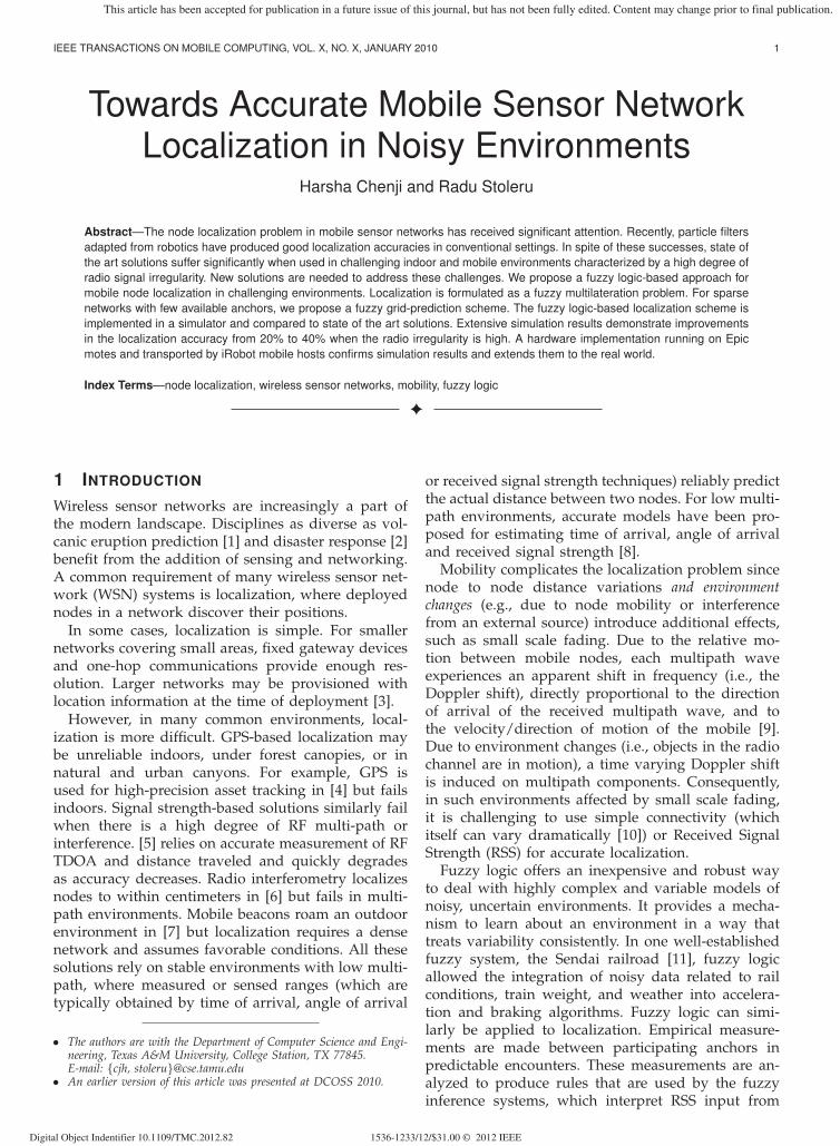
Fig. 1. (a) Illustration of radio patterns for two different degrees of radio irregularity (DoI); (b) the effect of DoI onlocalization error in MSL, MCL and Centroid; and (c) the effect of anchor density on localization error, at DoI=0.4,for MSL, MCL and Centroid.

unlocalized nodes and other anchors. The output ofthis process recovers the actual distance, compensatedfor variability in the local environment. This basictechnique is employed in two constituent subsystemsof FUZLOC - the Fuzzy Multilateration System (FMS)and the Fuzzy Grid Prediction System (FGPS). Thecontributions of this article are as follows:

• We formulate the mobile node localization prob-lem for noisy environments, as a fuzzy inferenceprocess.

• We present fuzzy multilateration, a componentof our fuzzy inference process, which obtains anode’s location from noisy RSS measurements,using fuzzy rule sets.

• We present a fuzzy grid prediction scheme, whichoptimizes our fuzzy inference process, under con-ditions of low anchor density.

• We demonstrate the feasibility of our proposedtechnique, through an implementation usingmote hardware hosted on iRobot.

• We perform extensive simulations and compareour solution with to state of the art algorithms,using both real-world and synthetic data.

This article is organized as follows. Section 2 mo-tivates our work. In Sections 3 and 4 we present ourfuzzy logic-based node localization framework, andthe node localization system design, respectively. Weevaluate the performance of our proposed node local-ization system in Section 5, including a real hardwareimplementation. We review related work in Section 6and conclude in Section 7. The Supplemental Materialcontains a detailed explanation of the fuzzificationprocess, a numerical example for fuzzy multilatera-tion, examples of fuzzy rulesets and an experimentshowing the effect of Monte Carlo sample size onlocalization accuracy.

2 MOTIVATION

This article is motivated by our interest in a local-ization technique for a mobile sensor network, de-

ployed in a harsh environment and a set of interest-ing/surprising results obtained from simulations oftwo state of the art localization techniques for mobilesensor networks, namely MCL [12] and MSL [13].We define a harsh environment as one in whichthe distance between sender and receiver cannot beaccurately determined from the RSS alone, due toenvironmental phenomena such as multipath prop-agation and interference.

For more complete problem formulation we men-tion that the aforementioned localization techniquesassume that given a set of mobile sensor nodes, asubset of nodes, called anchors, know their locationin a 2-dimensional plane. Also, nodes and anchorsmove randomly in the deployment area. Maximumvelocity of a node is bounded but the actual veloc-ity is unknown to nodes or anchors. Nodes do nothave any knowledge of the mobility model. Anchorsperiodically broadcast their locations. All nodes aredeployed in a noisy, harsh environment and they donot have any additional sensors except their radios.MCL gathers samples using Monte Carlo methodsand filters them using a particle filter, with the criteriabeing that each sample should be within range of a 1hop anchor (with respect to itself) while at the sametime, not being in range of a 2-hop anchor. Samplesare assigned weights over successive iterations. MSLimproves upon MCL by using criteria involving allneighbors and not just anchors. MSL is also adaptableto static scenarios if the nodes are allowed to exchangetheir samples and weights.

Using simulators developed by the authorsof [12] [13], we developed a scenario with highlyirregular radio ranges, typical of harsh indooror extremely obstructed outdoor environments.The irregularity in the radio range is modeled inthese simulators as a degree of irregularity (DoI)parameter [12]. The DoI represents the maximumradio range variation per unit degree change indirection. An example, depicted in Figure 1(a), whenDoI=0.4 the actual communication range is randomly



chosen from [0.6r, 1.4r].Simulation results, for a network of 320 nodes, 32

anchors deployed in a 500 × 500 grid and moving at0.2r (r, the radio range) are shown in Figures 1(b)and 1(c). Figure 1(b) demonstrates that the DoI pa-rameter has a significant negative effect on the local-ization accuracy. At DoI=0, MCL and MSL achievelocalization errors of 0.2r and 0.5r. With an increasein the DoI to 0.4, their localization error increases400%. More surprisingly, as depicted in Figure 1(c), ata high DoI value, an increase in the number of anchorshas a detrimental effect on localization accuracy. Thisresult is counter-intuitive since access to more an-chors implies that nodes have more opportunities toreceive accurate location information, as exemplifiedby the performance of Centroid (which computesthe location as the average of the coordinates of allanchors in its vicinity), in the same figure. A similarobservation is made in [7] although no further studywas performed. Our results and also those of [14],[15] suggest that large errors are detrimental to theMonte Carlo method since the samples get succes-sively polluted with time. In [15], a proposed Mixture-MCL method uses odometry to gather samples andthen uses sensor data to assign weights, enabling it torecover quickly from such errors, while [14] does thesame based on error correction based on learnt pathsand topological constraints. In the specific case ofMCL, the nodes used for filtering the samples may notbe actual neighbors because of the non-uniformity inthe radio range varies in every direction. The numberof polluted samples increases with increasing anchordensity. Simply increasing the size of the particle filterin MCL (to 1000 from the current value of 50) doesnot improve the accuracy significantly, as can be seenin Fig. 10 of [12].

3 A FUZZY LOGIC-BASED NODE LOCAL-IZATION FRAMEWORK

The challenges identified above were partially ad-dressed in recent work in sensor network node lo-calization [16], [17]. The authors create hybrid lo-calization mechanisms that make use of range-basedlocalization primitives (e.g., RSSI) to validate andimprove the accuracy of range-free techniques.

In a similar vein, we propose to formulate thelocalization problem as a fuzzy inference problem byusing RSSI to obtain distance, in a fuzzy logic-basedlocalization system where the concept of distance isvery loose, such as “High”, “Medium” or “Low”. Thecore intuition is that accurate ranges can be deter-mined by learning about the local RF environmentand developing rules based on this knowledge. Fuzzylogic provides a simple and computationally inexpen-sive way to accomplish this learning. In other, simi-larly dynamic scenarios like rail transportation [11]and photovoltaic power generation [18], fuzzy logic

(a) (b)

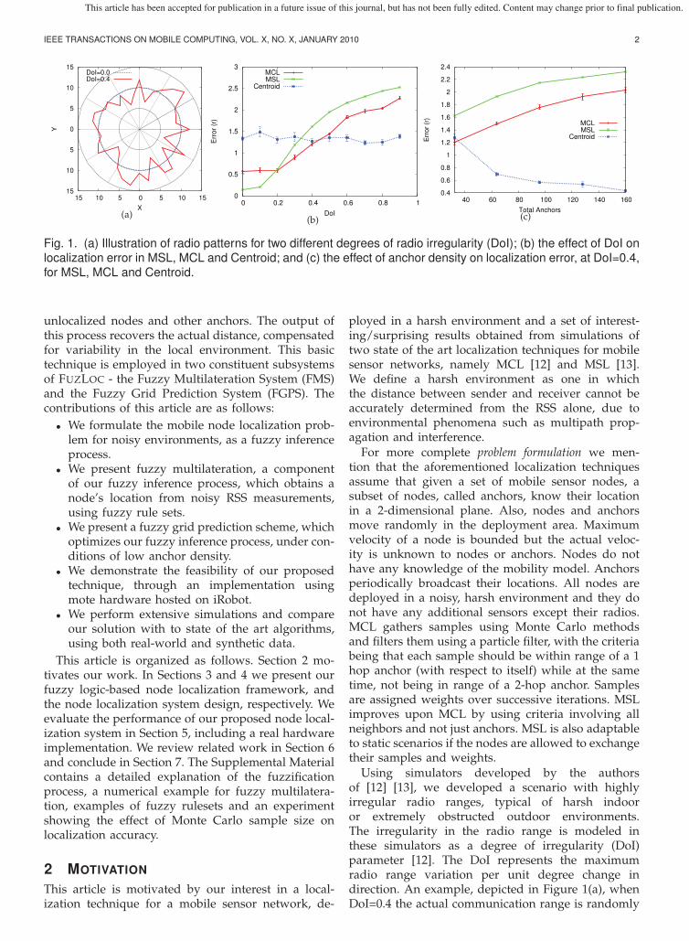
Fig. 2. (a) Representation of a fuzzy location, usingtwo triangular membership functions; and (b) a sensornode S with fuzzy coordinates X and Y , to be locatedusing three anchors at (x1, y1), (x2, y2) and (x3, y3).

provides mechanisms that allow simple systems tosmartly adapt to rapidly changing environments.

In our proposed fuzzy logic-based localization sys-tem, distances between a mobile sensor node andanchor nodes are fuzzified, and used, subsequently ina Fuzzy Multilateration procedure to obtain a fuzzylocation. In case two or more anchors are not availablefor performing localization using fuzzy multilater-ation, the sensor node employs a new technique,called fuzzy grid prediction, to obtain a location, albeitimprecise. In the Fuzzy Grid Prediction method, thenode uses ranging information from any available an-chor to compute distances to several fictitious “virtualanchors” which are assumed to be located in prede-termined grids or quadrants. This allows the node tolocate the grid/quadrant in which it is present.

In conventional localization schemes, the locationof a node is typically represented by two coordi-nates that uniquely identify a single point withinsome two-dimensional area. Localization using fuzzycoordinates follows a similar convention. The twodimensional location of a node is represented as apair (X,Y ), where both X and Y are fuzzy numbersand explained below. However, instead of a singlepoint, the fuzzy location represents an area where theprobability of finding the node is highest, as depictedin Figure 2(a). This section develops the theoreticalfoundation behind the computation of this fuzzy lo-cation, using imprecise and noisy RSSI measurements.

3.1 BackgroundFuzzy logic revisits classical set theory and modifiesit to have non-rigid, or fuzzy, set boundaries. Whereclassical set theory is concerned with collections ofdiscrete objects, a fuzzy set, sometimes called a fuzzybin, is defined by an associated membership functionμ, which describes the degree of membership 0 ≤μ(x) ≤ 1 of a crisp (regular) number x in the fuzzy set.The process of calculating the membership of a crispnumber for many fuzzy sets is called the fuzzificationprocess.



A fuzzy number is a special fuzzy bin where themembership is 1 at one and only one point. A fuzzynumber represents a multi-valued, imprecise quantityunlike a single valued traditional number. One popu-lar μ(x) function, is the triangular membership function:

μ(x) =

⎧⎪⎪⎨⎪⎪⎩

0 if x < a(x− a)/(b− a) if a ≤ x ≤ b(c− x)/(c− b) if b ≤ x ≤ c0 if x > c

(1)

where (a, b, c) defines a triangular bin. In this article,we chose a triangular membership function because,in addition to being a good substitute for the morewidely used Gaussian function, it has linear com-ponents only and computing membership is less re-source intensive, suitable for our resource constrainedsensor nodes. Since not all triangular memberships aresymmetric, we use the triangular function in its mostgeneral form. A comprehensive example can be foundin Supplemental Material, Section 1.

A fuzzy system translates a crisp input into a fuzzyoutput using a set of fuzzy rules which relate input andoutput variables in the form of an IF-THEN clause.Typically the IF clause contains the input linguisticvariable (e.g., RSSI) and the THEN clause containsthe output linguistic variable (e.g., DISTANCE). Anexample rule is:

IF RSSI is WEAK THEN DISTANCE is LARGE

3.2 Fuzzy MultilaterationAs shown in Figure 2(b), consider a node S that wantsto be localized, in the vicinity of three anchor nodesAj (j = 1, 3). Each anchor node is equipped with a setof fuzzy rules that map fuzzy RSSI values to fuzzydistance values:

Rule i: IF RSSI is RSSIi THEN DIST is Disti

where RSSIi and Disti are fuzzy linguistic variables(e.g. WEAK, MEDIUM , HIGH).

A fuzzy rule is created when two anchors can com-municate directly. Since anchors know their locations,they can find the distance between themselves andalso measure the RSSI. The anchors then fuzzify thecrisp RSSI and distance values into two fuzzy binsRSSIi and Disti respectively, through the process offuzzification. The chosen fuzzy bin is the one in whichthe crisp value will have the highest membershipvalue.

For a more general case, when the node S iswithin radio range of n anchors, the node localizationproblem can be formulated as a fuzzy multilaterationproblem. The following:

F1 = (X − x1)2 + (Y − y1)

2 −D21 = 0

...

Fn = (X − xn)2 + (Y − yn)

2 −D2n = 0

(2)

Fig. 3. The fuzzy inference process for an input RSSIvalue of -62dBm. In this example, the fuzzy rule basemaps this value through two rules: “Rule i” and “Rulej”. The dotted lines represent fuzzy inference: findingthe membership (vertical line on left), applying thesame membership to the output bin (horizontal linetowards right) and defuzzification (the lines intersectthe triangles to form a trapezoid).

defines a non-linear system of equations describingthe relation between the locations of the nodes andanchors and the distances among them. The variablesX , Y and Dk (k = 1, n) are fuzzy numbers rep-resenting the location of the node and the distanceto anchors respectively, while (xk, yk) (k = 1, n) arecrisp numbers representing the crisp location of theanchors. The objective is to minimize the mean squareerror over all equations.

3.2.1 Fuzzy InferenceA definition of the process of obtaining the fuzzydistance Dk between node and anchor is neededbefore solving the system of equations. This process,called fuzzy inference, transforms a crisp RSSI valueobtained from a packet sent by a node and receivedby an anchor into a fuzzy number Dk. Figure 3depicts an example for the fuzzy inference process. Asshown, an RSSI value of -62dBm has different mem-bership values μ(RSSI) for the fuzzy bins WEAKand MEDIUM . The two fuzzy bins, in this example,are mapped by a fuzzy rule base formed by two fuzzyrules:

Rule i: IF RSSI is MEDIUM THEN DIST isMEDIUMRule j: IF RSSI is WEAK THEN DIST is LARGE

These two fuzzy rules define the mapping from theRSSI fuzzy sets to the DIST fuzzy sets. As shown inFigure 3, the two fuzzy rules indicate the membershipμ(DIST ) in the DIST domain. Pi and Pj indicatethe center of gravity of the trapezoid formed by themapping of the RSSI into fuzzy bins MEDIUM andLARGE, respectively.

Typically, a single RSSI value triggers multiplefuzzy rules (the membership value of the crisp valuein the input bin of the fuzzy rule is non-zero), result-ing in multiple distance bins. Assume that the fuzzyrule base maps an RSSI value to a set of m fuzzyDist bins. The set of centers of gravity Pl (l = 1,m)is denoted by P = {P1, P2 . . . Pm}. The output fuzzynumber Dk is calculated as follows: First, calculate the



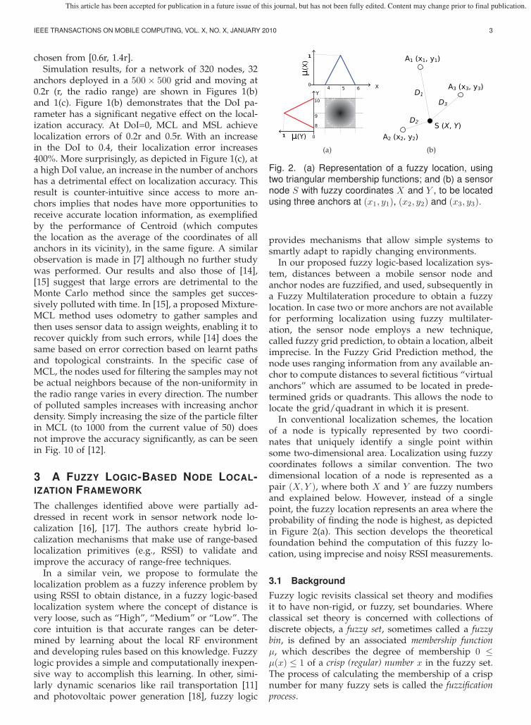
Fig. 4. Illustrating the multi-hop case for fuzzy multilat-eration: A node S localizes itself using A2 and A1.

centroid of all points in P - call it Pc. Next, take thecentroid of all points in P whose abscissa is less thanthat of Pc i.e., L = {Pn|x(Pn) ≤ x(Pc)}. Similarly, G ={Pn|x(Pn) ≥ x(Pc)} is the set of points whose abscissais greater than that of P . The abscissae of three pointsP , L and G represent the resulting fuzzy distance Dk,formally described as (subscript x denotes abscissa):

Dk = (a, b, c) =

((∑Ln

|L|)

x

, (Pc)x,

(∑Gn

|G|)

x

)(3)

This definition of obtaining a fuzzy number throughfuzzy inference produces a fuzzy number while giv-ing more “weight” to the centroid by eliminatingsome possibilities at the edge. To truly represent theresult one would need to compute a smooth andcontinuous function like the Gaussian membershipfunction, but the triangular approximation has theadvantage of reduced computation complexity.

Equation 3 limits its analysis to situations wherethe anchors and the node desiring localization are onehop from each other. This constraint limits the degreeof accuracy that can be achieved. Two hops providea good trade off between messaging overheads andaccuracy as explained later. Consider an anchor A2

(Figure 4) which is 2 hops away from a node S.Suppose that a regular node S1 and an anchor A1 areneighbors of both S and A2. The aim is now to findthe distance DSA2 . In a 2-dimensional space, a straightline between two points is also the shortest possible;hence a good approximation is the minimum of allknown distances between the 2 points. Applying thisfact, we can now calculate:

DSA2 = min(DSS1 +DS1A2 , DSA1 +DA1A2) (4)

The distances in Equation 4 are fuzzy values, as theresult of defuzzification by either A1 or A2 depend-ing on the sender. Addition of two triangular fuzzynumbers (a, b, c) and (d, e, f) is well known in fuzzylogic theory [19] to be the sum of their individualparameters:

(a, b, c) + (d, e, f) = (a+ d, b+ e, c+ f)

The smallest fuzzy number, to be computed inEquation 4 is simply the fuzzy number with thelowest center value [19]:

min((a, b, c), (d, e, f)) =

{(a, b, c) if min(b, e) = b

(d, e, f) if min(b, e) = e

The minimum of many fuzzy numbers can be re-cursively computed in the case of multi hop mul-tilateration; it is beyond the scope of this article.In order to solve the non-linear system of Equa-tions 2, in two fuzzy variables, the fuzzy variant ofthe iterative classical Newton method based on theJacobian matrix [20] is used. To accomplish this, thefuzzy numbers are expressed in their parametric formX = (X,X) where X and X are continuous boundednon-decreasing and non-increasing, respectively, func-tions. These functions effectively represent the “lefthalf” and “right half” of the membership function.

For a triangular membership function, such as de-fined in Equation 1, a parametric representation inr ∈ [0, 1] is:

X = (a+ (b− a)r, c− (c− b)r)

The system of Equations 2 is, therefore, representedin the parametric form. Without loss of generality,assume that X and Y are positive. Then, the systemcan be split into:

F1 = (X − x1)2 + (Y − y1)

2 −D12 = 0

...

Fn = (X − xn)2 + (Y − yn)

2 −Dn2 = 0

(5)

and

F1 = (X − x1)2 + (Y − y1)

2 −D12= 0

...

Fn = (X − xn)2 + (Y − yn)

2 −Dn2= 0

(6)

The Jacobian J is constructed as:

J =

⎡⎢⎢⎢⎢⎢⎣

F1XF1X

F1YF1Y

F1X F1X F1Y F1Y

... ... ... ...FnX

FnXFnY

FnY

FnX FnX FnY FnY

⎤⎥⎥⎥⎥⎥⎦ (7)

J =

⎡⎢⎢⎢⎣2(X − x1) 0 2(Y − y1) 0

0 2(X − x1) 0 2(Y − y1)... ... ... ...

2(X − xn) 0 2(Y − yn) 00 2(X − xn) 0 2(Y − yn)

⎤⎥⎥⎥⎦

Initial guesses of X and Y can be updated asfollows. For every iteration compute a matrix Δ:

Δ = [h(r) h(r) k(r) k(r)]T (8)

where h, h, k and k are defined as incremental updatesto the initial guess:

X(r) = X(r) + h(r)

X(r) = X(r) + h(r)

Y (r) = Y (r) + k(r)

Y (r) = Y (r) + k(r)

(9)



(a) (b)

Fig. 5. (a) A sensor S and the grid cells in its vicinity,is within radio range of anchor A3; and (b) averagedistance between sensor S and virtual anchor VAj .

The set of equations evaluated at the initial guessis:

F = [F1 F1 . . . Fn Fn]T (10)

The equation that connects them is Δ = −J−1F .The initial guess (X0, Y0) is computed from the av-erage of the coordinates of the anchors. Then, J andF are computed for this initial guess. The incrementalupdate Δ is calculated and applied to X and Y . J andF are computed for the new values and the processis repeated until Δ converges to 0 within ε.

3.3 Fuzzy Grid Prediction

The multilateration technique presented in the pre-vious section assumes the presence of a sufficientnumber of anchors, typically three or more. However,in mobile sensor networks with low anchor densities,it might frequently be the case that a node does nothave enough anchors for multilateration. To addressthis problem we extend our fuzzy logic-based local-ization framework to predict an area, e.g., a cell in agrid, where the node might be. The idea is inspiredfrom cellular systems [21]. We propose to virtualizethe anchors, so that a node is within a set of VirtualAnchors at any point in time. A Virtual Anchor isa fictitious anchor which is assumed to located at aknown, fixed location in the field of deployment, thedistance to which can be found in an approximateway from the node. In FUZLOC, we place virtualanchors at the center of every square cell that the fieldis divided into, as described below. The key idea isthat the nearer a node is to a virtual anchor, the morelikely it is that the node can be found in that cell.

Consider the area in which the network is deployedto be subdivided into a grid of G cells, as depicted inFigure 5(a). Denote the probability that a node S is ina cell j (j = 1 . . . G) by pj . To infer these probabilities,we construct a fuzzy system, whose input is thedistance dj between S and the center of cell j, andthe output is a scalar 0 < pj < 1 for each j. A rule inour fuzzy system is as follows:

Rule i: IF (DISTgrd1 is Di1) and . . . and(DISTgrdG is DiG) THEN (PROBgrd1 is Pi1) and. . . and (PROBgrdG is PiG)

where Dij is the fuzzy bin representing the distancebetween the node and the center of cell j, and Pij isthe fuzzy bin representing the probability that nodeS is in cell j.

For each rule i, we calculate pj by first fuzzifyingdj , applying it to the rule, and then defuzzifying theaggregate, as we described in Section 3.2.1. Once themost probable cell is found, the location of the nodecan be computed as the intersection between this celland a circle with a radius of r around the anchor.

It is paramount to remark that we can obtain pj onlyif the node S has at least one anchor in its vicinity,i.e., we can estimate Dij . The technique we proposefor estimating Dij is described in Section 3.3.1.

Before proceeding with the description of how wecompute Dij , we describe how to update pj when noanchor is in the vicinity of node S. Since there is ahigh correlation between the current and previous cella node is in, we construct a Recursive Least Squares(RLS) filter which predicts the cell in which the nodeS might be. For each cell j, we store a buffer xj(k) =[pj(k) pj(k−1) . . . pj(k−m)]T of m previous samples.We then define an RLS filter, updated whenever a newsample p(k + 1) is available, as:

xj(k + 1) = wTj (k)xj(k)

where wj(k) = wj(k − 1) + aj(k)gj(k) is a vector ofcoefficients, computed as follows:

aj(k) = xj(k)− wTj (k − 1)xj(k)

gj(k) = Pj(k − 1)xj(k){λ+ xTj (k)Pj(k − 1)xT

j (k)}−1

Pj(k) = λ−1Pj(k − 1)− gj(k)xTj (k)λ

−1Pj(k − 1)

where 0 ≤ λ ≤ 1 is the forgetfulness factor, a designparameter. Pj(0) is initialized to δIj , where I is theidentity matrix of size (m + 1) × (m + 1) and δ is atypically large value.

3.3.1 Calculation of Dij

The fuzzy system requires that we calculate the dis-tance from the node to the virtual anchor. We haveto find the average distance instead, because we donot know the node’s location. These average distancescan be calculated only when at least one anchor is inthe node’s vicinity.

Consider a node and a sole anchor A3 which isits neighbor, as illustrated in Figure 5(b). Take theset of all virtual anchors and discard the ones whichare at a distance of more than 2R from the anchorwhere R is the radio range of the anchor, since thisis the most distant virtual anchor the node can hearin the limiting case where the node is between theanchor and the virtual anchor. To calculate the averagedistance D from the node to a virtual anchor V Aj in



(a)

(b)

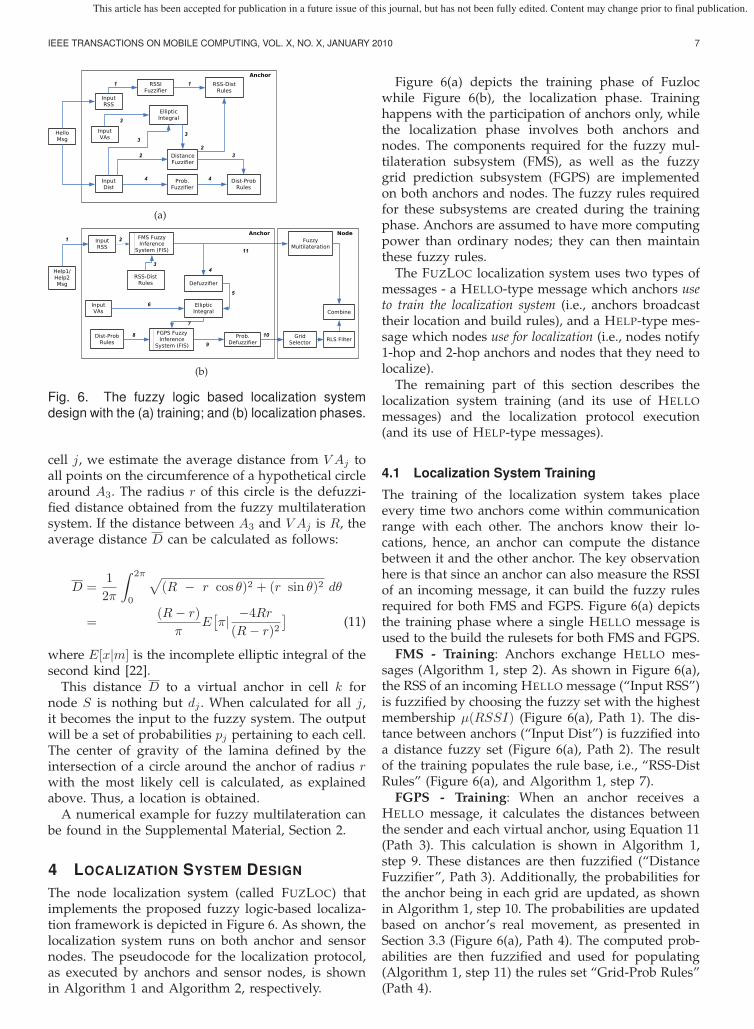
Fig. 6. The fuzzy logic based localization systemdesign with the (a) training; and (b) localization phases.

cell j, we estimate the average distance from V Aj toall points on the circumference of a hypothetical circlearound A3. The radius r of this circle is the defuzzi-fied distance obtained from the fuzzy multilaterationsystem. If the distance between A3 and V Aj is R, theaverage distance D can be calculated as follows:

D =1

2π

∫ 2π

0

√(R − r cos θ)2 + (r sin θ)2 dθ

=(R− r)

πE[π| −4Rr

(R− r)2]

(11)

where E[x|m] is the incomplete elliptic integral of thesecond kind [22].

This distance D to a virtual anchor in cell k fornode S is nothing but dj . When calculated for all j,it becomes the input to the fuzzy system. The outputwill be a set of probabilities pj pertaining to each cell.The center of gravity of the lamina defined by theintersection of a circle around the anchor of radius rwith the most likely cell is calculated, as explainedabove. Thus, a location is obtained.

A numerical example for fuzzy multilateration canbe found in the Supplemental Material, Section 2.

4 LOCALIZATION SYSTEM DESIGN

The node localization system (called FUZLOC) thatimplements the proposed fuzzy logic-based localiza-tion framework is depicted in Figure 6. As shown, thelocalization system runs on both anchor and sensornodes. The pseudocode for the localization protocol,as executed by anchors and sensor nodes, is shownin Algorithm 1 and Algorithm 2, respectively.

Figure 6(a) depicts the training phase of Fuzlocwhile Figure 6(b), the localization phase. Traininghappens with the participation of anchors only, whilethe localization phase involves both anchors andnodes. The components required for the fuzzy mul-tilateration subsystem (FMS), as well as the fuzzygrid prediction subsystem (FGPS) are implementedon both anchors and nodes. The fuzzy rules requiredfor these subsystems are created during the trainingphase. Anchors are assumed to have more computingpower than ordinary nodes; they can then maintainthese fuzzy rules.

The FUZLOC localization system uses two types ofmessages - a HELLO-type message which anchors useto train the localization system (i.e., anchors broadcasttheir location and build rules), and a HELP-type mes-sage which nodes use for localization (i.e., nodes notify1-hop and 2-hop anchors and nodes that they need tolocalize).

The remaining part of this section describes thelocalization system training (and its use of HELLOmessages) and the localization protocol execution(and its use of HELP-type messages).

4.1 Localization System Training

The training of the localization system takes placeevery time two anchors come within communicationrange with each other. The anchors know their lo-cations, hence, an anchor can compute the distancebetween it and the other anchor. The key observationhere is that since an anchor can also measure the RSSIof an incoming message, it can build the fuzzy rulesrequired for both FMS and FGPS. Figure 6(a) depictsthe training phase where a single HELLO message isused to the build the rulesets for both FMS and FGPS.

FMS - Training: Anchors exchange HELLO mes-sages (Algorithm 1, step 2). As shown in Figure 6(a),the RSS of an incoming HELLO message (“Input RSS”)is fuzzified by choosing the fuzzy set with the highestmembership μ(RSSI) (Figure 6(a), Path 1). The dis-tance between anchors (“Input Dist”) is fuzzified intoa distance fuzzy set (Figure 6(a), Path 2). The resultof the training populates the rule base, i.e., “RSS-DistRules” (Figure 6(a), and Algorithm 1, step 7).

FGPS - Training: When an anchor receives aHELLO message, it calculates the distances betweenthe sender and each virtual anchor, using Equation 11(Path 3). This calculation is shown in Algorithm 1,step 9. These distances are then fuzzified (“DistanceFuzzifier”, Path 3). Additionally, the probabilities forthe anchor being in each grid are updated, as shownin Algorithm 1, step 10. The probabilities are updatedbased on anchor’s real movement, as presented inSection 3.3 (Figure 6(a), Path 4). The computed prob-abilities are then fuzzified and used for populating(Algorithm 1, step 11) the rules set “Grid-Prob Rules”(Path 4).



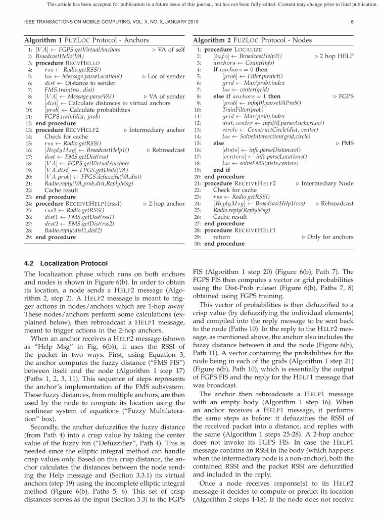
Algorithm 1 FUZLOC Protocol - Anchors1: [V A]← FGPS.getVirtualAnchors � VA of self2: BroadcastHello(VA)3: procedure RECVHELLO4: rss← Radio.getRSS()5: loc← Message.parseLocation() � Loc of sender6: dist← Distance to sender7: FMS.train(rss, dist)8: [V A]← Message.parseVA() � VA of sender9: [dist]← Calculate distances to virtual anchors

10: [prob]← Calculate probabilities11: FGPS.train(dist, prob)12: end procedure13: procedure RECVHELP2 � Intermediary anchor14: Check for cache15: rss← Radio.getRSS()16: [ReplyMsg]← BroadcastHelp1() � Rebroadcast17: dist← FMS.getDist(rss)18: [V A]← FGPS.getVirtualAnchors19: [V A.dist]← FPGS.getDists(VA)20: [V A.prob]← FPGS.defuzzify(VA.dist)21: Radio.reply(VA.prob,dist,ReplyMsg)22: Cache result23: end procedure24: procedure RECEIVEHELP1(rss1) � 2 hop anchor25: rss2← Radio.getRSS()26: dist1← FMS.getDist(rss1)27: dist2← FMS.getDist(rss2)28: Radio.reply(dist1,dist2)29: end procedure

4.2 Localization Protocol

The localization phase which runs on both anchorsand nodes is shown in Figure 6(b). In order to obtainits location, a node sends a HELP2 message (Algo-rithm 2, step 2). A HELP2 message is meant to trig-ger actions in nodes/anchors which are 1-hop away.These nodes/anchors perform some calculations (ex-plained below), then rebroadcast a HELP1 message,meant to trigger actions in the 2-hop anchors.

When an anchor receives a HELP2 message (shownas “Help Msg” in Fig. 6(b)), it uses the RSSI ofthe packet in two ways. First, using Equation 3,the anchor computes the fuzzy distance (“FMS FIS”)between itself and the node (Algorithm 1 step 17)(Paths 1, 2, 3, 11). This sequence of steps representsthe anchor’s implementation of the FMS subsystem.These fuzzy distances, from multiple anchors, are thenused by the node to compute its location using thenonlinear system of equations (“Fuzzy Multilatera-tion” box).

Secondly, the anchor defuzzifies the fuzzy distance(from Path 4) into a crisp value by taking the centervalue of the fuzzy bin (“Defuzzifier”, Path 4). This isneeded since the elliptic integral method can handlecrisp values only. Based on this crisp distance, the an-chor calculates the distances between the node send-ing the Help message and (Section 3.3.1) its virtualanchors (step 19) using the incomplete elliptic integralmethod (Figure 6(b), Paths 5, 6). This set of crispdistances serves as the input (Section 3.3) to the FGPS

Algorithm 2 FUZLOC Protocol - Nodes1: procedure LOCALIZE2: [info]← BroadcastHelp2() � 2 hop HELP3: anchors← Count(info)4: if anchors = 0 then5: [prob]← Filter.predict()6: grid← Max(prob).index7: loc← center(grid)8: else if anchors = 1 then � FGPS9: [prob]← info[0].parseVAProb()

10: TrainFilter(prob)11: grid← Max(prob).index12: dist, center ← info[0].parseAnchorLoc()13: circle← ConstructCircle(dist, center)14: loc← SolveIntersection(grid,circle)15: else � FMS16: [dists]← info.parseDistances()17: [centers]← info.parseLocations()18: loc← solveFMS(dists,centers)19: end if20: end procedure21: procedure RECEIVEHELP2 � Intermediary Node22: Check for cache23: rss← Radio.getRSS()24: [ReplyMsg]← BroadcastHelp1(rss) � Rebroadcast25: Radio.reply(ReplyMsg)26: Cache result27: end procedure28: procedure RECEIVEHELP129: return � Only for anchors30: end procedure

FIS (Algorithm 1 step 20) (Figure 6(b), Path 7). TheFGPS FIS then computes a vector or grid probabilitiesusing the Dist-Prob ruleset (Figure 6(b), Paths 7, 8)obtained using FGPS training.

This vector of probabilities is then defuzzified to acrisp value (by defuzzifying the individual elements)and compiled into the reply message to be sent backto the node (Paths 10). In the reply to the HELP2 mes-sage, as mentioned above, the anchor also includes thefuzzy distance between it and the node (Figure 6(b),Path 11). A vector containing the probabilities for thenode being in each of the grids (Algorithm 1 step 21)(Figure 6(b), Path 10), which is essentially the outputof FGPS FIS and the reply for the HELP1 message thatwas broadcast.

The anchor then rebroadcasts a HELP1 messagewith an empty body (Algorithm 1 step 16). Whenan anchor receives a HELP1 message, it performsthe same steps as before: it defuzzifies the RSSI ofthe received packet into a distance, and replies withthe same (Algorithm 1 steps 25-28). A 2-hop anchordoes not invoke its FGPS FIS. In case the HELP1message contains an RSSI in the body (which happenswhen the intermediary node is a non-anchor), both thecontained RSSI and the packet RSSI are defuzzifiedand included in the reply.

Once a node receives response(s) to its HELP2message it decides to compute or predict its location(Algorithm 2 steps 4-18). If the node does not receive



a response, it uses the RLS filter to predict the mostprobable grid it is in (Algorithm 2 steps 5-7). If thenode receives a response from one anchor, it com-putes the center of gravity of the area obtained byintersection between: a) the grid with the maximumprobability; and b) the circle with a center at theanchor location and with radius equal to the distancebetween the anchor and the node (Algorithm 2 steps9-14). If the node receives two or more responses, ituses fuzzy multilateration to iteratively compute itslocation (Algorithm 2, steps 16-18).

A node can also be on the receiving end of a HELP2message - when it is an intermediary node. In thiscase, the node first detects the RSSI of the receivedmessage (Algorithm 2 step 23) and then packages intoa HELP1 message and broadcasts it (Algorithm 2 step24). Any response(s) to this message will be sent backto the sender as a reply to the original HELP2 messagethat was sent by the node intending to localize. Anode ignores any HELP1 message it receives, since itis meant only for anchors (Algorithm 2 step 29).

5 PERFORMANCE EVALUATION

In this section, we first demonstrate that FUZLOCcan be implemented and run on real mote hardware,then show FUZLOC’s superior performance, whencompared with state of art solutions like MCL [12],MSL [13] and Centroid [23]. Owing to the rela-tively few number of robots, the difficulty in im-plementing MCL and MSL on real hardware (pleasenote that neither MSL, nor MCL have been im-plemented/evaluated on real hardware), controllingthe anchor and seed density and the physical spaceconstraints, we decided to compare performance ofFUZLOC with state of art solutions, in simulationsusing both empirical and synthetic data.

In the remaining part of this section we presentFUZLOC implementation on real-hardware, describethe empirical and synthetic RSSI-Distance mapping,and performance evaluation results.

5.1 System Implementation Validation

We implemented FUZLOC/FMS on EPIC motes run-ning TinyOS 2.1.1. Since the matrices involved inFMS are not always square and hence they cannotbe simply inverted, the fast and lightweight SVDbased pseudo inverse method [22] was implementedon the motes. Relevant portions of the GNU ScientificLibrary (GSL) were ported to the MSP430 architecturein order to achieve this goal. The result was a fastmethod of inverting matrices, providing 4 digits ofaccuracy when compared to a similar computation ona desktop PC. The 1,574 lines of code fit comfortablyin 18,726B.

A Fuzzy Inference System (FIS) consisting of atriangular rule set and center-average defuzzification

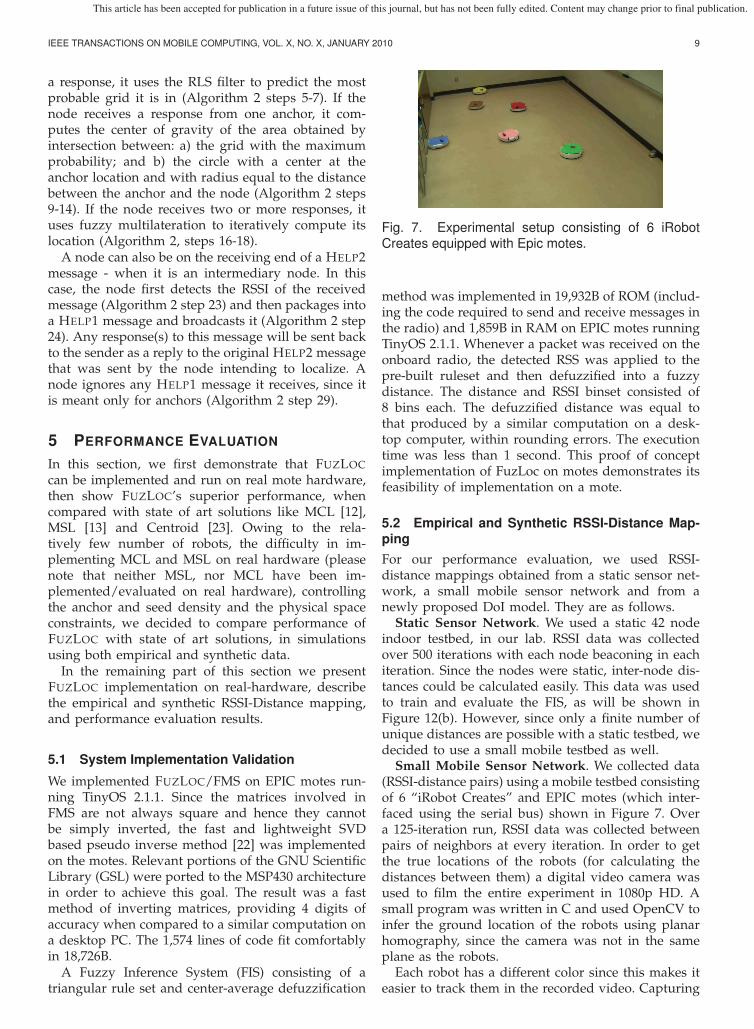
Fig. 7. Experimental setup consisting of 6 iRobotCreates equipped with Epic motes.

method was implemented in 19,932B of ROM (includ-ing the code required to send and receive messages inthe radio) and 1,859B in RAM on EPIC motes runningTinyOS 2.1.1. Whenever a packet was received on theonboard radio, the detected RSS was applied to thepre-built ruleset and then defuzzified into a fuzzydistance. The distance and RSSI binset consisted of8 bins each. The defuzzified distance was equal tothat produced by a similar computation on a desk-top computer, within rounding errors. The executiontime was less than 1 second. This proof of conceptimplementation of FuzLoc on motes demonstrates itsfeasibility of implementation on a mote.

5.2 Empirical and Synthetic RSSI-Distance Map-pingFor our performance evaluation, we used RSSI-distance mappings obtained from a static sensor net-work, a small mobile sensor network and from anewly proposed DoI model. They are as follows.

Static Sensor Network. We used a static 42 nodeindoor testbed, in our lab. RSSI data was collectedover 500 iterations with each node beaconing in eachiteration. Since the nodes were static, inter-node dis-tances could be calculated easily. This data was usedto train and evaluate the FIS, as will be shown inFigure 12(b). However, since only a finite number ofunique distances are possible with a static testbed, wedecided to use a small mobile testbed as well.

Small Mobile Sensor Network. We collected data(RSSI-distance pairs) using a mobile testbed consistingof 6 “iRobot Creates” and EPIC motes (which inter-faced using the serial bus) shown in Figure 7. Overa 125-iteration run, RSSI data was collected betweenpairs of neighbors at every iteration. In order to getthe true locations of the robots (for calculating thedistances between them) a digital video camera wasused to film the entire experiment in 1080p HD. Asmall program was written in C and used OpenCV toinfer the ground location of the robots using planarhomography, since the camera was not in the sameplane as the robots.

Each robot has a different color since this makes iteasier to track them in the recorded video. Capturing



15

10

5

0

5

10

15

15 10 5 0 5 10 15

Y

X

A

B

C

DoI=0.0

DoI=0.4

(a)

-120

-110

-100

-90

-80

-70

-60

-50

-40

-30

0 20 40 60 80 100 120R

SS

I (d

Bm

)Distance

DoI=0.4

DoI=0

(b)

Fig. 8. (a) The DoI model with three points of interest:although A and B are equally distant, their RSS valuesdiffer significantly in our EDoI model; and (b) RSSI vs.distance for the radio model used in the simulator, atDoI=0.4 and 0.

the radio effects caused by mobility and the orienta-tion of the antennae on the motes in real time was themain motivation behind the experiment. The groundlocations of the robots at each step is then used to inferthe actual distance between nodes for every measuredRSS between nodes. These RSSI-distance pairs werethen used to train and evaluate the FIS as will beshown in Figure 12(c) and described below.

EDoI Model. Since our fuzzy logic-based localiza-tion technique makes use of the RSSI, we extendedthe DoI model [24]. In order to adjust the simulatedRSSI for both the actual radio range and log-normalfading, we developed the EDoI model. It combinesthe general log-normal fading model with the DoImodel [24]. In Figure 8(a), OA and OC are the radioranges for the antenna situated at the origin O, in twodifferent directions as evaluated by the DoI model.Assume that the receiver sensitivity is -94dBm i.e., if atransmitter with similar characteristics as the receiveris situated at A or C, then the RSSI at the origin willbe -94dBm. To calculate the RSSI at a point B in thesame direction as C where OA = OB, we apply alog-normal fading model with the reference distanceas OC, such that the RSSI at point C is -60dBm. Notethat the RSSI at A is -94dBm, whereas the RSSI at anequidistant point B in a different direction is -60dBm.On top of this, additive random noise (uniformlydistributed, min = -20dB, max = 20dB) is appliedto the calculated RSSI. This procedure is done everytime a node uses this model to simulate an RSSI,ensuring randomness in both temporal and spatialrandomness. Formally:

RSSI(d) = Silog10 d

log10[r(1 +DoI × rand())](12)

where Si is the receiver sensitivity, r is the ideal radiorange, DoI is the radio degree of irregularity and randis a random number U [0, 1].

5.3 Simulation ParametersThrough extensive simulations, we compare our so-lution with MCL [12], MSL [13] and Centroid [23],

since we wanted to evaluate our solution against non-centralized solutions for non-static networks, bothMonte Carlo based (MCL, MSL) and simple (Cen-troid). A theoretical “Perfect FUZLOC” method showsthe theoretical optimum FUZLOC can reach, by simplybypassing the FIS and considering the actual distancebetween nodes. The problem of not having enoughanchors in the vicinity of nodes causes non-zero errorfor Perfect FUZLOC. Data gathered from the the staticand small mobile sensor network has been used toevaluate the FIS system. Thus, the FIS system isevaluated using simulated RSSI-Distance data as wellas data from the two experiments described before.

We simulate a set (N) of 320 sensor nodes deployedin a 500×500 area. Of the 320 nodes deployed, 32nodes are designated anchors (set S). The radio range(r) of a node is 50 and the default DoI is 0.4. Wechose these simulation parameters for consistencywith results reported in [12], [13]. The default receiversensitivity (Si) is -94dBm, and a plot depicting thepredicted RSSI by our EDoI model, is shown inFigure 8(b). The default maximum node velocity isto 0.2r. This velocity has been reported in [12] tobe optimal. We investigate the performance of allsolutions for node velocities up to 0.5r. The nodevelocity is an important parameter since MCL andMSL use it as a filtering criterion in their particlefilters. The default setup uses 10 fuzzy triangular binsand the defuzzification method is center-average. Thefuzzy location is defuzzified into a crisp location byconsidering only the center values of the abscissa andthe ordinate. The fuzzy bins for distance and RSSI areuniformly distributed between (0, r) and (−40, −100)respectively, with the width of each bin being twicethe separation between peaks of two adjacent fuzzybins. With 10 distance and RSS bins, there are 100different combinations that can be seen in a RSS-Distruleset. Rules encountered more frequently tend toaffect the output more than infrequent ones becausethe defuzzification method involves centroids corre-sponding to the output bin of each rule. A sampleset of fuzzy RSS-Dist rules has been provided in theSupplemental Material, Section 3.

5.4 Radio Irregularity

We performed simulations for different DoI valueswith all other parameters kept constant. Figure 9depicts our results, indicating the deterioration inlocalization accuracy of MCL, MSL and Centroid. Theeffect of compounded errors due to polluted sampleshas been investigated as the “kidnapped robot prob-lem” [14] in robot localization. The kidnapped robottest verifies whether the localization algorithm is ableto recover from localization failures, as signified bythe sudden change in location due to “kidnapping”.It has been shown [14] that such uncorrected algo-rithms collapse when the observed sample is far from



0.2

0.4

0.6

0.8

1

1.2

1.4

1.6

1.8

2

0.1 0.2 0.3 0.4 0.5

Err

or

(r)

Max. Velocity (r)

MCL

Centroid

MSL

FuzLoc

Perfect FuzLoc

(a)

0

0.5

1

1.5

2

2.5

20 40 60 80 100 120 140 160

Err

or

(r)

Total Anchors

MCL

MSL

Centroid

FuzLoc

Perfect FuzLoc

(b)

0.2

0.4

0.6

0.8

1

1.2

1.4

1.6

1.8

2

100 200 300 400 500 600

Err

or

(r)

Total Nodes

MCL

MSL

Centroid

FuzLoc

Perfect FuzLoc

(c)

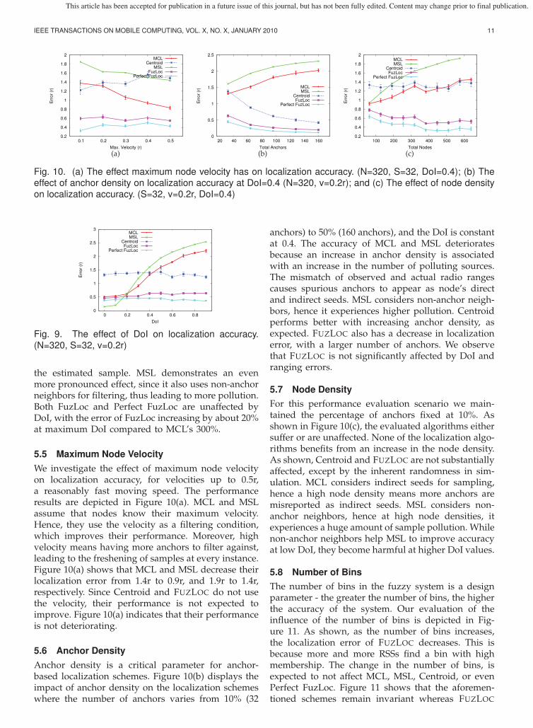
Fig. 10. (a) The effect maximum node velocity has on localization accuracy. (N=320, S=32, DoI=0.4); (b) Theeffect of anchor density on localization accuracy at DoI=0.4 (N=320, v=0.2r); and (c) The effect of node densityon localization accuracy. (S=32, v=0.2r, DoI=0.4)

0

0.5

1

1.5

2

2.5

3

0 0.2 0.4 0.6 0.8

Err

or

(r)

DoI

MCL

MSL

Centroid

FuzLoc

Perfect FuzLoc

Fig. 9. The effect of DoI on localization accuracy.(N=320, S=32, v=0.2r)

the estimated sample. MSL demonstrates an evenmore pronounced effect, since it also uses non-anchorneighbors for filtering, thus leading to more pollution.Both FuzLoc and Perfect FuzLoc are unaffected byDoI, with the error of FuzLoc increasing by about 20%at maximum DoI compared to MCL’s 300%.

5.5 Maximum Node VelocityWe investigate the effect of maximum node velocityon localization accuracy, for velocities up to 0.5r,a reasonably fast moving speed. The performanceresults are depicted in Figure 10(a). MCL and MSLassume that nodes know their maximum velocity.Hence, they use the velocity as a filtering condition,which improves their performance. Moreover, highvelocity means having more anchors to filter against,leading to the freshening of samples at every instance.Figure 10(a) shows that MCL and MSL decrease theirlocalization error from 1.4r to 0.9r, and 1.9r to 1.4r,respectively. Since Centroid and FUZLOC do not usethe velocity, their performance is not expected toimprove. Figure 10(a) indicates that their performanceis not deteriorating.

5.6 Anchor DensityAnchor density is a critical parameter for anchor-based localization schemes. Figure 10(b) displays theimpact of anchor density on the localization schemeswhere the number of anchors varies from 10% (32

anchors) to 50% (160 anchors), and the DoI is constantat 0.4. The accuracy of MCL and MSL deterioratesbecause an increase in anchor density is associatedwith an increase in the number of polluting sources.The mismatch of observed and actual radio rangescauses spurious anchors to appear as node’s directand indirect seeds. MSL considers non-anchor neigh-bors, hence it experiences higher pollution. Centroidperforms better with increasing anchor density, asexpected. FUZLOC also has a decrease in localizationerror, with a larger number of anchors. We observethat FUZLOC is not significantly affected by DoI andranging errors.

5.7 Node DensityFor this performance evaluation scenario we main-tained the percentage of anchors fixed at 10%. Asshown in Figure 10(c), the evaluated algorithms eithersuffer or are unaffected. None of the localization algo-rithms benefits from an increase in the node density.As shown, Centroid and FUZLOC are not substantiallyaffected, except by the inherent randomness in sim-ulation. MCL considers indirect seeds for sampling,hence a high node density means more anchors aremisreported as indirect seeds. MSL considers non-anchor neighbors, hence at high node densities, itexperiences a huge amount of sample pollution. Whilenon-anchor neighbors help MSL to improve accuracyat low DoI, they become harmful at higher DoI values.

5.8 Number of BinsThe number of bins in the fuzzy system is a designparameter - the greater the number of bins, the higherthe accuracy of the system. Our evaluation of theinfluence of the number of bins is depicted in Fig-ure 11. As shown, as the number of bins increases,the localization error of FUZLOC decreases. This isbecause more and more RSSs find a bin with highmembership. The change in the number of bins, isexpected to not affect MCL, MSL, Centroid, or evenPerfect FuzLoc. Figure 11 shows that the aforemen-tioned schemes remain invariant whereas FUZLOC



0

5

10

15

20

25

30

35

40

45

50

0 5 10 15 20 25 30 35 40 45 50

Ou

tpu

t

Input

Actual

Ideal

(a)

0

50

100

150

200

250

300

350

0 50 100 150 200 250 300 350

Ou

tpu

t

Input

Actual

Ideal

(b)

0

2

4

6

8

10

12

14

16

18

20

0 2 4 6 8 10 12 14 16 18 20

Outp

ut

Input

Actual

Ideal

(c)

Fig. 12. (a) Performance of the FMS FIS subsystem, with the test input on the X axis and the inferred distanceson the Y axis; (b) Performance based on real data gathered from our indoor testbed; (c) Performance based onreal data gathered from our mobile testbed consisting of 6 iRobots.

0.4

0.6

0.8

1

1.2

1.4

1.6

1.8

2 4 6 8 10

Err

or

(r)

Fuzzy Bins

MCL

Centroid

MSL

FuzLoc

Perfect FuzLoc

Fig. 11. The effect of the number of fuzzy bins onlocalization accuracy. (N=320, S=32, v=0.2r, DoI=0.4)

experiences decreasing error with an increase in thenumber of bins.

5.9 Fuzzy Inference System PerformanceFigure 12(a) shows the performance of the FIS engineevaluated using RSSI-distance data generated by theEDoI model, while Figure 12(b) does the same usingdata from our static testbed and finally, Figure 12(c)uses data from the small mobile testbed. Input dis-tance is on the X axis while the Y axis marks the centervalue of the defuzzified output distance. After train-ing the system with 30 random RSS-Distance pairs,RSS values deduced from distances were fed intothe system so that a distance could be inferred. Thestraight line shows the ideal case. In order to quantifythe accuracy, the root mean squared (RMS) error wascalculated and normalized to the radio range. Thevalues are remarkably similar: for the EDoI dataset itwas 0.156, for the static network dataset it was 0.182and for the small mobile testbed it was 0.166. In away, these numbers reinforce the equivalence of thesimulated and real indoor static/mobile radio models,while proving the effectiveness of the EDoI model.

5.10 OverheadA typical FIS does not require much storage capacity.If there were 8 bins, for example, a single byte couldrepresent a bin. Hence, each FMS rule requires just 2Bof storage. Typically, an anchor creates approximately

30 rules during the period of deployment whichtranslates to 60B of storage. The FGPS FIS however,requires 50B for each rule (25 bins in the input, 25in the output). Note that regular nodes do not storerules, only the anchors store rules. Moreover, due tothe nature of the triangular bin shapes, simple calcu-lations are required in order to fuzzify and defuzzify.The only caveat is the inversion of matrices that isrequired. As for the filter, the node does not constructa filter for all possible cells, since it usually visits amaximum of 4 cells per iteration. Hence, the storagerequired by a 3-order filter on each non-anchor nodewill be (288×4×4×3) = 13,824B. MCL requires at least50 samples for low localization error. Each samplerequires a weight. Centroid does not store any his-tory and thus has the smallest storage requirement.Amorphous stores announcements made by the an-chors which are flooded throughout the network. Ifthere are 320 nodes, 32 of which are anchors, MCLrequires each node to store 50 samples. Each samplehas an abscissa and an ordinate, each of at least4B. Hence, MCL requires around (50×4×2×320) =128,000B. Fuzzy on the other hand requires around1,500B for FGPS and around 60 for FMS, with 13,824Bfor the filters, which sums up to (1,560×32 + 13,824)= 63,744B which is roughly 50% of the storage MCLrequires, and even less than what MSL requires, sinceMSL mains closeness values.

The communication overhead for 2-hop anchor dis-covery is the same as that of MCL, and less that ofMSL (since MSL needs to exchange samples in addi-tion to anchor discovery). When FuzLoc uses only 1-hop anchors, the communication overhead required issignificantly lower since all that is needed is a simplebroadcast. Still, FuzLoc performs better than MCL ascan be seen in [25]. Therefore, systems desiring lessercommunication overhead should use anchors within1 hop only, while those desiring higher accuracy needto consider anchors within 2 hops. In no state will thecommunication overhead required by FuzLoc exceedthat of MCL or MSL.



0.2

0.3

0.4

0.5

0.6

0.7

0.8

0.9

0 0.2 0.4 0.6 0.8

Err

or

(r)

DoI

1hop, 20%

2hop, 20%

1hop, 15%

2hop, 15%

Fig. 13. Comparison of 1 and 2 hop FUZLOC variantsat seed densities of 15% (S=48) and 20% (S=64) in a320 node (N) network across multiple DoIs.

5.11 Single hop and Dual hop FMS

Figure 13 compares the 1-hop and 2-hop variants ofFUZLOC. Being a multilateration based method, thepresence of a sufficient number of anchors in a node’svicinity is crucial to reducing the error in locationestimation. A simple way to ensure this is to increasethe percentage of anchors in the network. However,the addition of anchors may be cost prohibitive. Asimpler way and less costly solution is to consideranchors which are two hops away. The additional costincurred for this solution is higher messaging over-head. Instead of traveling over a single hop, localiza-tion request broadcasts must take two hops to reachthe outer anchors. Replies are consolidated, so noadditional messaging is incurred in the reply phase.The number of additional transmissions required varybased on node and anchor density. Figure 13 showsthat merely considering the 2-hop anchors results ina much lower error due to the increased number ofanchors, than introducing more anchors, across allDoIs. Note that although the number of messagesincreases, the error is more than halved.

6 RELATED WORK

Range-based localization methods require an estimate ofthe distance or angle between two nodes to localizeand may operate in both absolute and relative coor-dinate systems. Methods requiring specialized hard-ware include precise measurement of acoustic phasedifference [26], optical sensors/reflectors [27]. Typicaldrawbacks for these methods include higher com-putational loads, increased node size, higher energyconsumption and increased cost. A lighter weightsolution uses fuzzy logic to locate cellular phones in ahexagonal grid in a cellular network [28]. It assumesa fixed number of anchors but handles mobility verywell. The computation and refining are not suitablefor a resource-constrained computation platform likea MicaZ node. This was the inspiration for this work.

[29] uses precise infra-red ranging in combinationwith a grid based fuzzy logic approach. [30] pro-poses using RSS-Distance fuzzy rules to perform crisplocalization, when there are anchors placed at the

four corners of the deployment area. In [31], time-of-arrival and RSS data is fused together using Bayesianinference, following which fuzzy optimization is usedto compute a crisp location. Compared to the abovethree works, FuzLoc does not assume the presence ofadditional sensing capabilities [29] [31] and provideslocalization solutions when there are less than threeanchors [30] as well as computing the location as anarea, a feature not found in previous work.

Range-free localization methods are typically used insystems where connectivity is the metric of choiceand actual geographic distance is less important. Hopcounting is a technique frequently used in thesescenarios, where the distance between two nodes isinferred from the number of hops a packet takesand is based on some assumed or measured averagehop length [32]. A major drawback is that it fails innetworks with irregular topologies such as those witha concave shape [33]. Mobility incurs large overheadsince all hop counts must be refreshed frequently.

[34] uses hypothesis testing to infer the location ofa node, by using RSS PDF distributions gathered byanchors nodes through surveying. The fundamentaldifference between fuzzy logic and hypothesis testingis that while the former gathers learned intelligenceand applies it to a given input, the latter tests allpossibilities using tools like the Generalized Likeli-hood Ratio Test (GLRT). In [34], building each PDF bysurveying requires a large sample space. The compu-tation involved in building the PDFs and performingthe tests is not suitable for embedded devices unlikeFuzLoc. The complexity associated with hypothesistesting increases with increasing number of anchorsas well as the deployment area, since there are moretests to be conducted (with multiple tests, the acceptedhypothesis from the previous test is used in the nexttest). With fuzzy logic, the number of rules increaseswith the anchor density but is independent of de-ployment area. Fuzzy rules require only storage whilehypothesis testing requires computation and storage.

This paper extends previous work done on FUZ-LOC [25]. Major changes include system implemen-tation on Epic motes, FIS evaluation using mobileiRobots, a distributed protocol, system integration andmost importantly, evaluation of and support for fuzzymultilateration using multi hop anchors.

7 CONCLUSIONSWe have proposed FUZLOC, a fuzzy logic based lo-calization method suitable for wireless sensor nodesthat are mobile in noisy, harsh environments. Theconstituent systems use fuzzy multilateration and agrid predictor to compute the location of a node asan area. The RSS is cast into bins which encode theimprecision; these bins are subsequently used in ourmathematical framework. We remark here that thecase of static anchors, considered by neither MCL, norMSL, will be investigated in future work.



Our method has been evaluated based on a varietyof metrics. They prove that our method is resistantto high DoI environments while providing a lowlocalization error without any extra hardware. Onlyanchors need to have a slightly higher storage require-ment. A deployment with more anchors at high DoIdecreases the error. The ability to localize using bothsingle-hop and two-hop anchors greatly increasesthe variety of topologies where localization succeeds.The system implementation proves that the algorithmfunctions well on resource constrained devices.

Acknowledgements: The authors thank D. Evansand M. Rudafshani for simulator code, and S. Georgefor help and feedback during manuscript preparation.This work was supported, in part, by NSF grantsgrants 0923203, 1127449.

REFERENCES[1] G. Werner-Allen, K. Lorincz, M. Ruiz, O. Marcillo, J. Johnson,

J. Lees, and M. Welsh, “Deploying a wireless sensor networkon an active volcano,” Internet Computing, IEEE, March-April2006.

[2] S. George, W. Zhou, H. Chenji, M. Won, Y. O. Lee, A. Pazar-loglou, R. Stoleru, and P. Barooah, “Distressnet: a wireless adhoc and sensor network architecture for situation managementin disaster response,” Communications Magazine, IEEE, March2010.

[3] T. He, S. Krishnamurthy, L. Luo, T. Yan, L. Gu, R. Stoleru,G. Zhou, Q. Cao, P. Vicaire, J. Stankovic, T. Abdelzaher, J. Hui,and B. Krogh, “VigilNet: an integrated sensor network systemfor energy-efficient surveillance,” ACM Trans. Sens. Netw.,2006.

[4] D. Balakrishnan, A. Nayak, P. Dhar, and S. Kaul, “Efficientgeo-tracking and adaptive routing of mobile assets,” in HPCC,2009.

[5] H. Akcan, V. Kriakov, H. Bronnimann, and A. Delis, “GPS-free node localization in mobile wireless sensor networks,” inMobiDE, 2006.

[6] B. Kusy, J. Sallai, G. Balogh, A. Ledeczi, V. Protopopescu,J. Tolliver, F. DeNap, and M. Parang, “Radio interferometrictracking of mobile wireless nodes,” in MobiSys, 2007.

[7] A. Baggio and K. Langendoen, “Monte carlo localization formobile wireless sensor networks,” Ad Hoc Netw., 2008.

[8] D. Puccinelli and M. Haenggi, “Multipath fading in wire-less sensor networks: measurements and interpretation,” inIWCMC, 2006.

[9] T. S. Rappaport, Wireless Communications: Principles and Practice(2nd Edition), 2nd ed. Prentice Hall, Jan. 2002.

[10] K. Whitehouse, C. Karlof, and D. E. Culler, “A practical evalu-ation of radio signal strength for ranging-based localization,”Mobile Computing and Communications Review, 2007.

[11] H. Oshima, S. Yasunobu, and S.-i. Sekino, “Automatic trainoperation system based on predictive fuzzy control,” in IEEEAI for Industrial Applications, 1988.

[12] L. Hu and D. Evans, “Localization for mobile sensor net-works,” in MobiCom, 2004.

[13] M. Rudafshani and S. Datta, “Localization in wireless sensornetworks,” in IPSN, 2007.

[14] S. Engelson and D. McDermott, “Error correction in mobilerobotmap learning,” in ICRA, 1992.

[15] S. Thrun, D. Fox, W. Burgard, and F. Dellaert, “Robust montecarlo localization for mobile robots,” Artificial Intelligence, vol.128, no. 1-2, pp. 99–141, 2000.

[16] K. Yedavalli, B. Krishnamachari, S. Ravula, and B. Srinivasan,“Ecolocation: a sequence based technique for rf localization inwireless sensor networks,” in IPSN, 2005.

[17] Z. Zhong and T. He, “Achieving range-free localization be-yond connectivity,” in SenSys, 2009.

[18] J. Li and H. Wang, “Maximum power point tracking of pho-tovoltaic generation based on the fuzzy control method,” inSUPERGEN, 2009.

[19] A. Kaufman, M. Gupta, and B. Esposito, Introduction to FuzzyArithmetic: Theory and Applications. Van Nostrand ReinholdCompany, 1991.

[20] J. Shokri, “On systems of fuzzy nonlinear equations.” Appl.Math. Sci. (Ruse), 2008.

[21] X. Shen, J. W. Mark, and J. Ye, “User mobility profile pre-diction: an adaptive fuzzy inference approach,” Wirel. Netw.,2000.

[22] M. Abramowitz and I. A. Stegun, Handbook of Mathemati-cal Functions with Formulas, Graphs, and Mathematical Tables.Dover Publications, 1964.

[23] N. Bulusu, J. Heidemann, and D. Estrin, “GPS-less low costoutdoor localization for very small devices,” IEEE PersonalCommunications Magazine, 2000.

[24] T. He, C. Huang, B. M. Blum, J. A. Stankovic, and T. Abdelza-her, “Range-free localization schemes for large scale sensornetworks,” in MobiCom, 2003.

[25] H. Chenji and R. Stoleru, “Mobile sensor network localizationin harsh environments,” in DCOSS, 2010.

[26] M. Maroti, P. Volgyesi, S. Dora, B. Kusy, A. Nadas, AkosLedeczi, G. Balogh, and K. Molnar, “Radio interferometricgeolocation,” in SenSys, 2005.

[27] R. Stoleru, P. Vicaire, T. He, and J. A. Stankovic, “Stardust: aflexible architecture for passive localization in wireless sensornetworks,” in SenSys, 2006.

[28] X. Shen, J. W. Mark, and J. Ye, “Mobile location estimationin cdma cellular networks by using fuzzy logic,” Wirel. Pers.Commun., 2002.

[29] A. Dharne, J. Lee, and S. Jayasuriya, “Using fuzzy logicfor localization in mobile sensor networks: simulations andexperiments,” in ACC, 2006.

[30] S.-Y. Chiang and J.-L. Wang, “Localization in wireless sensornetworks by fuzzy logic system,” in KES, 2009.

[31] S.-L. Dong, J.-M. Wei, T. Xing, and H.-T. Liu, “Constraint-based fuzzy optimization data fusion for sensor networklocalization,” in SKG, 2006.

[32] D. Niculescu and B. Nath, “DV Based Positioning in Ad HocNetworks,” Telecommunication Systems, January 2003.

[33] C. Wang and L. Xiao, “Sensor localization in concave environ-ments,” ACM Trans. Sen. Netw., 2008.

[34] I. C. Paschalidis, K. Li, and D. Guo, “Model-free probabilisticlocalization of wireless sensor network nodes in indoor envi-ronments,” in MELT, 2009.

Harsha Chenji Harsha Chenji joined theDepartment of Computer Science and Engi-neering at Texas A&M University in August2007. He is currently a Ph.D. candidate underthe guidance of Dr. Radu Stoleru, after grad-uating with a M.S. (Computer Engineering)degree in Dec 2009. He obtained his Bache-lor of Technology in Electrical and Electron-ics Engineering from the National Instituteof Technology Karnataka, Surathkal, India inMay 2007.

Dr. Radu Stoleru Dr. Radu Stoleru is cur-rently an assistant professor in the Depart-ment of Computer Science and Engineeringat Texas A&M University. He received hisPh.D. in computer science from the Univer-sity of Virginia in 2007, and the ComputerScience Outstanding Graduate Student Re-search Award in 2007. Dr. Stoleru’s researchinterests are in deeply embedded wirelesssensor systems, distributed systems, em-bedded computing, and computer network-

ing. He has authored or co-authored over 60 conference and journalpapers with over 1,700 citations.



Supplemental Materials

Towards Accurate Mobile Sensor NetworkLocalization in Noisy Environments

Harsha Chenji and Radu Stoleru

F

1 BACKGROUND ON FUZZIFICATION

The process of calculating the membership of a crispnumber for many fuzzy sets is called the fuzzificationprocess.

A fuzzy number is a special fuzzy bin where themembership is 1 at one and only one point. A fuzzynumber represents a multi-valued, imprecise quantityunlike a single valued traditional number. One popu-lar µ(x) function, is the triangular membership function:

µ(x) =

0 if x < a(x− a)/(b− a) if a ≤ x ≤ b(c− x)/(c− b) if b ≤ x ≤ c0 if x > c

(1)

where (a, b, c) defines a triangular bin. As shown inFigure 1, the WEAK fuzzy set can be represented as(-90, -70, -50) and MEDIUM as (-70, -50, -30). A crispnumber, RSSI = -55dBm has a membership of 0.25 inWEAK and 0.75 in MEDIUM .

WEAK MEDIUM STRONG1

0.75

0.25

µ(R

SSI)

RSSI [dbm]

-90 -70 -50 -30 -100

Fig. 1. Fuzzification of a crisp value of -55dBm intofuzzy bins WEAK, MEDIUM and STRONG havingtriangular membership functions: WEAK, MEDIUMand STRONG with degrees of membership of 0.25,0.75 and 0.0 respectively.

2 FUZZY MULTILATERATION NUMERICALEXAMPLE

A numerical example elaborates the concept of fuzzymultilateration. Consider three anchors forming an

isosceles triangle (Figure 2) - (0, 0), (10, 0) and (5, 15).Let the node to be localized be at the centroid whichis (5, 5). The actual distances to the anchors wouldbe 5

√2, 5

√2, 10 respectively. Assume that because of

defuzzification, the node calculates the fuzzy dis-tances as (6, 7, 8), (6, 7, 8), (9, 10, 11) respectively. Thethe system of equations can be expressed as:

F1 = (X − 0)2 + (Y − 0)2 − (6, 7, 8)2 = 0

F2 = (X − 10)2 + (Y − 0)2 − (6, 7, 8)2 = 0

F3 = (X − 5)2 + (Y − 15)2 − (9, 10, 11)2 = 0

The actual fuzzy location (X,Y ) of the node is(5, 5, 5), (5, 5, 5). Assume the initial guess of (X,Y ) tobe (5, 6, 7), (5, 6, 7) for the purposes of demonstration,which by the process of convergence should ideallyyield the actual location. The parametric form wouldthen be (5 + r, 7− r). Expanding only F1 for brevity,

F1 = (X − 0)2 + (Y − 0)2 − (6, 7, 8)2

F1 = (X − 0)2 + (Y − 15)2 − (6, 7, 8)2

which can then be simplified to

F1 = (5 + r − 0)2 + (5 + r − 0)2 − (6 + r)2

F1 = (7− r − 0)2 + (7− r − 15)2 − (8− r)2

Similarly the Jacobian can now be constructed as(first 2 rows only):

J =

[2(5 + r) 0 2(5 + r) 0

0 2(7− r) 0 2(7− r)

]The pseudo-inverse of a matrix with symbolic el-

ements is computationally expensive, especially forembedded sensor nodes. Instead of inverting J whichcontains a symbolic element r, two non-symbolicinverses can be computed (for r = 0 and r = 1)and the results combined. This alternate computationincurs a loss of accuracy because the solution will bea perfect triangular fuzzy number and not a fuzzy


1

32

10

7.07 7.07

Fig. 2. Three anchors and a node used in the numeri-cal example.

number with little variation. However, the accuracylost is extremely small.

A simple substitution of r = 0 and r = 1 in J andF yields:

∆0 = J−10 F0 and ∆1 = J−1

1 F1

Given a solution (X,Y ) expressed in simple formas (xA, xB , xC) and (yA, yB , yC), then:

∆0 =

δxA

δxC

δyAδyC

and ∆1 =

δxB

δxB

δyBδyB

(3)

where δxA is the incremental update to xA. This isobvious since the left half of any fuzzy number inparametric form (a + (b − a)r) evaluates to a whenr = 0. The same argument holds for the right half. Af-ter this step, the new (xA, xB , xC) and (yA, yB , yC) arethe input for the next iteration. The process is repeateduntil sufficient accuracy is obtained. Upon runningour algorithm for 10 iterations with the above initialguess, the final location of the node was calculatedas (5.0, 5.0, 5.0), (4.72, 4.97, 5.14). The value that wouldhave been used for comparison with algorithms thatdo not compute an area as a node’s location will be thecenter values of the two fuzzy numbers, i.e, (5, 4.97).

3 FUZZY RULESETS EXAMPLE

Table 1 shows a summary of the fuzzy RSS-Dist rulesencountered during simulation, on a randomly chosenanchor. The DoI at the time of rule capture was 0.4.The bin indexes refer to the values in an increasingorder. The RSSI bin with the lowest index captures thelowest RSS values (-100dBm) while the distance bincounterpart captures the smallest distance (0-0.1R).

We see that rules with a high distance bin indextypically have a low RSSI bin index and vice versa.This is representative of the fact the higher the dis-tance, lower is the RSSI and vice versa. The first tenrules stored on this node are shown below:

Rule 0 : If RSS is RSSI0, then DIST is Dist7Rule 1 : If RSS is RSSI0, then DIST is Dist6

Fuzzy Dist Bin Index0 1 2 3 4 5 6 7 8 9

Fuzz

yR

SSI

Bin

Inde

x 0 0 0 0 0 0 4 6 4 0 01 0 0 0 5 11 14 13 7 1 02 0 0 3 21 10 3 0 0 0 03 0 3 7 1 0 0 0 0 0 04 0 2 0 0 0 0 0 0 0 05 0 1 0 0 0 0 0 0 0 06 1 0 0 0 0 0 0 0 0 07 0 0 0 0 0 0 0 0 0 08 1 0 0 0 0 0 0 0 0 09 0 0 0 0 0 0 0 0 0 0

TABLE 1Distribution of fuzzy RSS-Dist rules, with the RSS binindex (vertical) and the Dist bin index (horizontal), for

a total of 117 rules.

0.2

0.4

0.6

0.8

1

1.2

1.4

1.6

1.8

2

0 100 200 300 400 500E

rro

r (r

)Sample Size

MCL

Centroid

FuzLoc

Perfect FuzLoc

MSL

Fig. 3. The effect of the number of samples on local-ization accuracy. (N=320, S=32, v=0.2r, DoI=0.4)

Rule 2 : If RSS is RSSI0, then DIST is Dist5Rule 3 : If RSS is RSSI0, then DIST is Dist6Rule 4 : If RSS is RSSI0, then DIST is Dist6Rule 5 : If RSS is RSSI0, then DIST is Dist6Rule 6 : If RSS is RSSI0, then DIST is Dist5Rule 7 : If RSS is RSSI0, then DIST is Dist7Rule 8 : If RSS is RSSI0, then DIST is Dist7Rule 9 : If RSS is RSSI0, then DIST is Dist6

4 EFFECT OF SAMPLE SIZE ON LOCALIZA-TION ACCURACY

Increasing the sample size for Monte Carlo based lo-calization algorithms typically reduces the localizationerror. However, there is a storage requirement for eachnode in storing the samples. The effect of sample sizeon MCL and MSL is shown in Figure 3. As the samplesize increases from 1 to around 150, localization errordecreases for MCL but fails to decrease noticeablyonce the sample size is increased further. A similartrend is observed for MSL with the exception that thecutoff size is around 100 samples. The default samplesize for both MCL and MSL is 50, in keeping withthe choice of the respective authors. At 400 samples,FuzLoc’s error is less than half of both MCL and MSL.

Storage overhead for MCL increases linearly withthe number of samples. As discussed in Section 5.10of the main article, MCL requires 128,000B of stor-age when each node stores 50 samples, compared to63,744B for FuzLoc. When the sample size is increased


to 100, the storage requirement is doubled (100%increase) whereas the error decreases by only 3%.For 400 samples, a 700% increase in storage require-ment facilitates a 9.8% decrease in error (baseline of50 samples). This experiment therefore demonstratesthat an increase in sample size does not justify theimprovement in accuracy when storage overhead isconsidered.

ieee transactions on mobile computing, vol. x, no. x, january 2010

Documents