IEEE TRANSACTIONS ON SMART GRID, 2017 1

A Data-Driven Methodology for Probabilistic WindPower Ramp Forecasting

Mingjian Cui, Member, IEEE, Jie Zhang, Senior Member, IEEE, Qin Wang, Member, IEEE, VenkatKrishnan, Member, IEEE, and Bri-Mathias Hodge, Senior Member, IEEE

Abstract—With increasing wind penetration, wind powerramps (WPRs) are currently drawing great attention to balancingauthorities, since these wind ramps largely affect power systemoperations. To help better manage and dispatch the wind power,this paper develops a data-driven probabilistic wind powerramp forecasting (p-WPRF) method based on a large numberof simulated scenarios. A machine learning technique is firstadopted to forecast the basic wind power forecasting scenario andproduce the historical forecasting errors. To accurately modelthe distribution of wind power forecasting errors (WPFEs), ageneralized Gaussian mixture model (GGMM) is developed andthe cumulative distribution function (CDF) is also analyticallydeduced. The inverse transform method based on the CDF isused to generate a large number of forecasting error scenarios.An optimized swinging door algorithm (OpSDA) is adopted toextract all the WPRs from the complete set of wind powerforecasting scenarios. The p-WPRF is generated based on allgenerated scenarios under different weather and time conditions.Numerical simulations on publicly available wind power datashow that the developed p-WPRF method can predict WPRswith a high level of reliability and accuracy.

Index Terms—Gaussian mixture model, probabilistic windpower ramp forecasting, scenario generation, wind power ramps.

NOMENCLATURE

A. Sets, Parameters, Variables, and Functions:cov(·) Covariance function.erf(·) Gaussian error function.f(·), F (·) PDF and CDF of the GGMM.gi(·) Probability distribution function of the ith Gaus-

sian model.h Predefined parameter to obtain the constant in

the GGMM CDF.i, G , NG Index, set, and total number of Gaussian models.j, X , NX Index, set, and total number of WPFEs.k Iteration number.m, n, v, t Index of time periods in the forecasting horizon.

m, n, v, t=1, 2, 3, ..., Tfh.r, z Random number.s, Nsc Index and total number of forecasting scenarios.xj , pj The jth actual WPFE and its actual probability.x Sampled random WPFE.yt, yt Measured value and deterministic forecasting

value of wind power at time t.ACE Average coverage error.AIS Average interval score.

M. Cui and J. Zhang are with the Department of Mechanical Engineering,the University of Texas at Dallas, Richardson, TX 75080, USA, e-mail:(mingjian.cui, jiezhang@utdallas.edu).

Q. Wang, V. Krishnan, and B.-M. Hodge are with the National RenewableEnergy Laboratory (NREL), Golden, CO 80401, USA, e-mail: (qin.wang,venkat.krishnan, bri.mathias.hodge@nrel.gov).

Manuscript received, 2017.

C Constant in an indefinite integral.It Indicator of PICP in the reliability metric.Jωij , J

µij , J

σij Elements of Jacobian matrix of the ith Gaussian

model and the jth forecasting error.Lαt , Uαt Lower and upper bounds of PIs.PDFA Actual PDF value of WPFEs.PICP PI coverage probability.PINC PI nominal confidence.Rj Residual of the jth WPFE.RL(·) Ramp rule of a wind power ramp.S1, S2 Objective function of the NLS method and dy-

namic programming in OpSDA.Sc Score function of the length of a time interval.Tfh Maximum forecasting horizon.β1−α/2 Critical value of standard Gaussian distribution.λ1, λ2 Range parameters to control the trust-region size

and the correlation of random variables.ε Stopping threshold for the RNGc.δ Interval score rewarding the PIs.φ Tolerance value for ramp duration forecasts.1–α Nominal coverage probability of PIs.µi, M Expected value of the ith Gaussian model and

the set.σm,n Exponential covariance function of multivariate

normal random number generator.σi, Σ Standard deviation of the ith Gaussian model

and the set.σ2t , σ2

yt, σ2

ε Variance of the total prediction errors, modeluncertainty, and noise data.

ωi, Ω Weight coefficient of the ith Gaussian model andthe set.

∆(·) Increment of a variable as a step size.Φ(·) Standard normal distribution function.B. Matrices and Vectors:Γ Vector of overall parameter matrix of GGMM.Jω,Jµ,Jσ,J

Jacobian matrix of ω, µ, and σ, and the overallJacobian matrix of all parameters.

∆ω,∆µ,∆σ,∆p

Incremental matrices of ω, µ, σ, and actualprobability values.

MMND,ΣMND

Mean value and covariance matrices of the mul-tivariate normal distribution.

I. INTRODUCTION

LARGE fluctuations in wind speed in a short time pe-riod can cause significant wind power ramps (WPRs)

and threaten the power system’s reliability [1]–[3]. WPRscan generally be divided into up-ramp, down-ramp, or non-ramp periods. This is becoming more challenging for systemoperators as larger wind power penetrations are seen in powersystems worldwide [4].

IEEE TRANSACTIONS ON SMART GRID, 2017 2

A number of statistical and machine learning methods havebeen developed in the literature to forecast wind power rampsat multiple forecasting horizons. For instance, Liu et al. [5] de-veloped a hybrid forecasting model to combine an orthogonaltest with support vector machine. Cutler et al. [6] forecastedwind power ramps and evaluated the efficiency of the WindPower Prediction Tool (WPPT) and the Mesoscale LimitedArea Prediction System (MesoLAPS) for ramp forecasting.Greaves et al. [7] forecasted up-ramps and down-ramps withuncertain start times and incorporated a numerical weatherprediction (NWP) model to reduce the forecasting errors.However, most of existing methods focus on the deterministicramp forecasting. Probabilistic wind power ramp forecasting(p-WPRF) is expected to provide more information on forecastuncertainties, and thus produce better system schedules forbalancing authorities. Among the few p-WPRF studies [8],Taylor [9] used a multinomial logit structure and categoricaldistribution to estimate the ramp event probabilities for differ-ent thresholds. Li et al. [10] provided additional probabilisticinformation for wind ramp occurrences by a logistic regressiontechnique.

Both the prevalent probabilistic and statistical scenarioforecasts can be used for wind power ramp forecasting.Probabilistic forecasts consider the intrinsic uncertainty in thewind power generation (or WPR) process, and give moreinformation on the forecasted wind power and WPRs thanthe simple point forecasts [11]. However, they neglect theinterdependence structure of forecast errors among look-aheadtimes, and cannot be practically used in the time-dependentand multi-stage decision-making processes, such as the designof trading strategies in a multi-market environment. Statisticalscenario forecasts mainly rely on the most recent informa-tion about the interdependence structure of the predictionerrors [11]. However, they should respect the probabilisticforecasts of the next time period. The intrinsic uncertainty inthe wind power generation (or WPR) process and the proba-bilistic view of the forecasting problem are not considered instatistical scenario forecasts [11]. Pinson et al. [12] evaluatedthe quality of statistical scenario forecasts of short-term windpower generation. Ma et al. [13] proposed a statistical scenarioforecast method considering the information of forecast errordistribution and fluctuation distribution of short-term windpower generation. In this paper, we consider the advantagesof both the probabilistic and statistical scenario forecasts.Probabilistic forecasts of WPR aim to provide informationabout the WPRF uncertainty. Statistical scenario forecastsof WPR aim to provide the time-dependent and multi-stageWPRFs that can be used in the decision-making processes.

To bridge the gap in ramp forecasting, we seek to addresstwo critical questions for balancing authorities with the in-creasing WPRs integrated into power systems. Is it possibleto quantitatively evaluate the probabilistic information of windramp occurrences, such as the ramp duration or start-time?What is the impact of different conditions on the probabilisticforecasting of WPRs, such as weather conditions (wind speed)or times of a day? This paper develops a p-WPRF method tocharacterize different key ramp features in different conditions.The main innovations and contributions of this paper include:

(i) developing a novel generalized Gaussian mixture model(GGMM) to fit the probability density function (PDF) of windpower forecasting errors (WPFEs); (ii) designing a statisticalscenarios based p-WPRF model by using the WPFE scenariosand a novel WPR detection algorithm; and (iii) calculatingand analyzing the probabilistic metrics of ramp features underdifferent weather and time conditions.

The overall procedure of the developed p-WPRF method-ology consists of four major steps. First, multiple sets ofdeterministic wind power forecasts are generated by a machinelearning method. Second, a novel GGMM distribution modelis developed to fit the actual PDF of WPFEs with a satisfactoryaccuracy, and the inverse transform method of GGMM isadopted to generate a large number of WPFE scenarios. Then,an optimized swinging door algorithm (OpSDA) is used toextract all the forecasting WPRs in each wind power fore-casting scenario that is generated by adding the baseline windpower forecast series with a random WPFE scenario. Finally,a suite of probabilistic forecasting metrics are calculated andcompared for ramping features under different conditions.

The organization of this paper is given as follows. InSection II, a WPFE scenario generation method is developed.In Section III, the methodology of p-WPRF and evaluationmetrics are presented. Case studies and results analysis per-formed on publicly available wind power data are discussedin Section IV. Concluding remarks and future work aresummarized in Section V.

II. WPFE SCENARIO GENERATION

The developed WPFE scenario generation is based on amachine learning technique to first forecast the basic windpower forecasting scenario and calculate the historical WPFEs.Then a generalized Gaussian mixture model (GGMM) is usedto fit the PDF of forecasting errors. The CDF is analyticallydeduced. The inverse transform method based on the CDF isused to generate a large number of WPFE scenarios.

Recently, the Gaussian mixture model (GMM) has beenwidely used to fit the distributions of wind power genera-tion [14], [15], load [16], and WPFEs [17], [18]. However,parameters of the GMM distribution are estimated by theexpectation maximization (EM) algorithm which is strictlyconstrained by three constraints: (i) all the weights of mixturecomponents must be nonnegative; (ii) the sum of all weightsequals one; and (iii) the integral of each mixture component(standard normal distribution) equals one. For the developedGGMM, the non-linear least square (NLS) method is firstutilized to estimate all the parameters. All the aforementionedthree constraints in the GMM are not required any more in theGGMM, which means more mixture Gaussian components,even with negative weights, can be integrated in a moregeneralized way.

A. Analytical Expression of the GGMM PDF

The basic wind power forecasts are generated using thesupport vector machine (SVM) that has been widely usedin the forecasting community. WPFEs are then calculatedand recorded as the deviation between the basic wind powerforecasts and the corresponding actual wind power. A GGMM

IEEE TRANSACTIONS ON SMART GRID, 2017 3

GGMM1 with one Gaussian component

GGMM2 with two Gaussian components

NLS

GGMM with Gaussian components

GGMM with Gaussian components

Parameters 1

NLS Parameters 2

NLS Parameters 1

NLS Parameters

PDF1

PDF2

PDF

PDF

Actual PDF

Euclidean distance

Optimal number of Gaussian

components,

Stage I Stage II

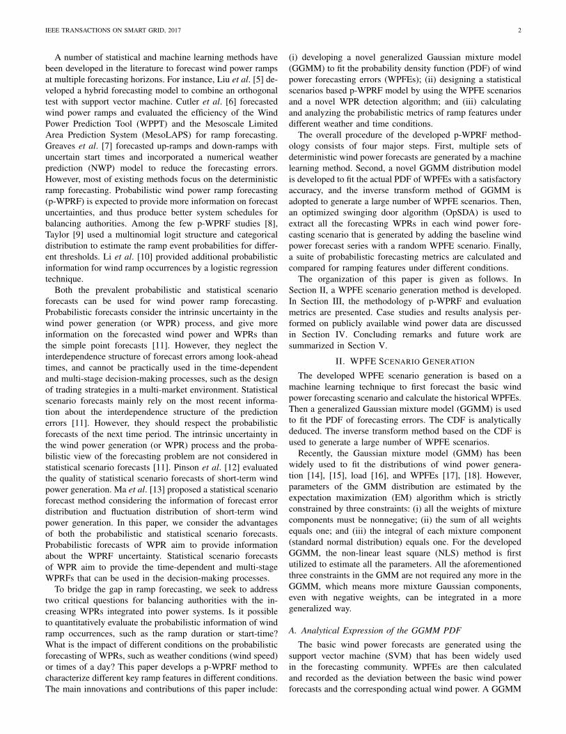
Fig. 1. Procedure of the two-stage optimization model.

distribution [14], [16], [19] is used to fit the PDF of WPFEs.The GGMM is a probabilistic model that assumes all the datapoints are generated from a mixture of a finite number of Gaus-sian distributions with multiple parameters. It is characterizedby the number of mixture components, weights, mean values,and standard deviations of each component, and formulatedas:

f(xj |NG; Γ) =

NG∑i=1

ωigi(xj |µi, σi), ∀xj ∈X ,∀i ∈ G (1)

where Γ defines a mixture component of the GGMM, i.e., Γ =ωi, µi, σiNG

i=1. The function of each component g (x|µ, σ)conforms to a Gaussian function, given by:

g(x|µ, σ) = e−(x−µ)2

2σ2 (2)

A two-stage optimization model is constructed to estimateall the parameters of f , i.e., NG, ωi, µi, and σi. In StageI, the objective is to estimate parameters for the GGMMcomponents using the NLS method. In Stage II, the objectiveis to determine the optimal number of components.

1) Stage I: The parameters of each GGMM are estimatedby using the NLS method. For each GGMM, the number ofGaussian components is a constant, as shown in the left part ofFig. 1. The PDF of GGMM is simplified as f(xj |NG; Γ)

NG−−→f(xj |Γ). This stage aims to determine the expected value (ormean value) set M (µi ∈ M), the standard deviation set Σ(σi ∈ Σ), and the weight coefficient set Ω (ωi ∈ Ω). TheNLS method using the trust-region algorithm [20] is adoptedto estimate parameters (ω, µ, and σ) of mixture componentsof the GGMM. Given a set of data points for WPFEs (x)and their actual probabilities (p), i.e., (x1, p1), ..., (xj , pj), ...,(xNX

, pNX), the objective function, S1, of the NLS aims to

minimize the sum of the squares of fitting residuals, given by:

S1 =

NX∑j=1

R2j =

NX∑j=1

[pj − f(xj |Γ)

]2(3)

Taking the mean value as an example, the minimum valueof S1 occurs when the gradient is zero, given by:

∂S1

∂µi= 2

NX∑j=1

Rj∂Rj∂µi

= −2

NX∑j=1

Rj∂f(xj |Γ)

∂µi= 0 (4)

Since the model contains 3×NG parameters, there are 3×NG gradient equations. Then, each mean value of the GGMM,µi, is refined iteratively by the successive approximation:

µi ≈ µk+1i = µki + ∆µi (5)

At each iteration, the GGMM is linearized by approximatingto a first-order Taylor series expansion:

f(xj |Γ) ≈ f(xj |Γk) +

NG∑i=1

∂f(xj |Γk)

∂ωi∆ωi

+

NG∑i=1

∂f(xj |Γk)

∂µi∆µi +

NG∑i=1

∂f(xj |Γk)

∂σi∆σi

(6)

The set of the derivatives ∂f(xj |Γk)/∂ωi, ∂f(xj |Γk)/∂µi,and ∂f(xj |Γk)/∂σi constitutes the Jacobian matrix, J. Eachderivative is analytically deduced by:

Jωij =∂f(xj |Γk)

∂ωi= e−

(xj−µki )2

2(σki)2 (7)

Jµij =∂f(xj |Γk)

∂µi=ωki (xj − µki )

(σki )2e−

(xj−µki )2

2(σki)2 (8)

Jσij =∂f(xj |Γk)

∂σi=ωki (xj − µki )2

(σki )3e−

(xj−µki )2

2(σki)2 (9)

J = [Jω Jµ Jσ]T, ∀Jωij ∈ Jω,∀Jµij ∈ Jµ,∀Jσij ∈ Jσ (10)

Since the iterative residuals are given by: ∆pj = pj −f(xj |Γk), the original residuals are rearranged by:

Rj = [pj − f(xj |Γk)] + [f(xj |Γk)− f(xj |Γ)]

= ∆pj −NG∑i=1

Jωij∆ωi −NG∑i=1

Jµij∆µi −NG∑i=1

Jσij∆σi(11)

Then substituting these expressions in (7)–(11) into thegradient equations in (4), we can rearrange and get the normalequations:

NX∑j=1

NG∑i=1

Jµij(Jωij∆ωi+J

µij∆µi+J

σij∆σi)=

NX∑j=1

Jµij∆pj (12)

NX∑j=1

NG∑i=1

Jωij(Jωij∆ωi+J

µij∆µi+J

σij∆σi)=

NX∑j=1

Jωij∆pj (13)

NX∑j=1

NG∑i=1

Jσij(Jωij∆ωi+J

µij∆µi+J

σij∆σi)=

NX∑j=1

Jσij∆pj (14)

The normal equations are written in the matrix notation:

JTJ

∆ω∆µ∆σ

= JT∆p (15)

Since the estimated initial parameters may be far from theoptimum, Equation (15) is improved by using the trust-regionalgorithm [20], given by:

[JTJ + λ1diag(JTJ)]

∆ω∆µ∆σ

= JT∆p (16)

where diag(JTJ) is the diagonal matrix with the same di-agonal as JTJ and λ1 is used to control the trust-region

IEEE TRANSACTIONS ON SMART GRID, 2017 4

size. Comparing with the line search algorithm, the trustregion algorithm can be used in the non-convex approximateproblems (or ill-conditioned problems) due to the boundednessof the trust regions of estimated initial parameters. Thisadvantage makes the trust region algorithm reliable and robustwith strong convergence properties [21].

2) Stage II: After estimating the parameters of each mix-ture component of the GGMM, the second stage aims todetermine the optimal number of mixture components, NG,opt,by minimizing the Euclidean distance between the actual PDF,PDFA, and the PDF of the GGMM, f , i.e., f(xj |NG)

NG,opt−−−−→f(xj), as shown in the right part of Fig. 1. The objectivefunction is formulated as:

min

√ ∑xj∈X

[f(xj |i)− PDFA]2, i = 1, 2, ...,NG (17)

B. Analytical Expression of the GGMM CDF

The cumulative distribution, F , is another essential statisticmetric to generate WPFE scenarios due to its monotonicity,which is analytically expressed as:

F (x|NG; Γ) =

∫ x

−∞

NG∑i=1

ωie− 1

2

[t−µiσi

]2dt

=

NG∑i=1

[√π

2ωiσierf(

µi − xσi

)

]+ C

(18)

erf(x) =2√π

∫ x

0

e−t2

dt (19)

where Equation (18) is an indefinite integral with a constantC, which can be solved by (20). Since WPFEs are normalizedinto the range [0, 1], it can be derived that F (x < 0) = 0and F (x > 1) = 1. Hence, we use a predefined parameter byheuristics [h ∈ (−∞, 0) ∪ (1,+∞)] to obtain the constant Cbased on the theory of the integral [22], given by:

C =

−

NG∑i=1

[√π2 ωiσierf

(h−µiσi

)], h < 0

1−NG∑i=1

[√π2 ωiσierf

(h−µiσi

)], h > 1

(20)

C. Random WPFE Generation Using GGMM

To sample a random WPFE, x, we design a random numbergenerator (RNG) based on the GGMM (RNG-GGMM). Theinverse transform method has been widely used to generaterandom numbers from a specific probability distribution [23],[24]. In this paper, the RNG-GGMM method utilizes theinverse function of the GGMM CDF, formulated as:

x = F−1 [F (x|NG; Γ)]

= F−1

NG∑i=1

[√π

2ωiσierf(

µi − xσi

)

]+ C

(22)

However, the inverse function in (22) cannot be analyticallydeduced. Alternatively, we use the Newton-Raphson method toobtain a numerial solution of the inverse CDF of the GGMMdistribution. The Newton-Raphson method has been used tosample the inverse CDF of the Student’s t distribution [25].

Algorithm 1: Newton-Raphson method for generating therandom number of WPFEs.

1 Initialization: obtain a random point (r ∈ [0, 1]) andevenly partition the WPFE, x, into N regions([xn, xn]Nn=1). Decide the region where r is:

2 if F (xn) < r < F (xn) then3 Return n, x0 = xn; and the approximation x1 is

calculated when k = 0, by:

xk+1 =xk −F (xk)− rF ′(xk)

= xk −F (xk)− rf(xk)

=xk −

NG∑i=1

[√π2 ωiσierf(µi−xkσi

)]

+ C− r

NG∑i=1

ωie− 1

2

[xk−µiσi

]2 (21)

4 end5 Output the random number of one forecasting error:6 for Iteration k from 1 to 100 do7 if |xk − xk−1| < ε then8 The sampled forecasting error is returned: x≈xk;9 else

10 The iterative process is repeated using (21).11 end12 end

The pseudocode of the forecasting error generation process isillustrated in Algorithm 1. The process repeats until the rangeis smaller than the stopping threshold ε, given by:

|xk − xk−1| < ε (23)

where ε is set as 1×10−8.A random number z is generated by the multivariate normal

random number generator, and uniformed by the standardnormal distribution, given by:

Φ (z)=

∫ z

−∞

1√2πe−

t2

2 dt, Φ (z) ∈ [0, 1] (24)

The multivariate normal random number generator mvnrndin MATLAB is then applied to generate Nsc scenarios witha forecasting horizon Tfh using the multivariate normal distri-bution (MND), z∼N (MMND,ΣMND). MMND is defined asa zero Nsc-by-Tfh matrix. ΣMND is a Tfh-by-Tfh symmetricpositive semi-definite matrix, formulated by:

ΣMND =

σ1,1 σ1,2 · · · σ1,Tfh

σ2,1 σ2,2 · · · σ2,Tfh

...... σm,n

...σTfh,1 σTfh,2 · · · σTfh,Tfh

(25)

where the covariance σm,n has been modeled by an exponen-tial covariance function in [12] and defined as:

σm,n = cov(rm, rn) = e−|m−n|λ2 , 0 ≤ m,n ≤ Tfh (26)

where λ2 is used to control the strength of the correlation ofrandom variables rm and rn.

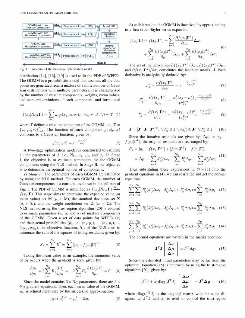
The forecasting error scenarios are generated by setting a to-tal number of Nsc, with a specific forecast horizon of Tfh (e.g.,day-ahead, hours-ahead, or minutes-ahead). A large set of

IEEE TRANSACTIONS ON SMART GRID, 2017 5

Algorithm 1:

Inverse Transform

Method

Multivariate Normal Random

Numbers Generator

Forecasting Error [p.u.]

0

0.2

0.4

0.6

0.8

1.0

0

0.2

0.4

0.6

0.8

1.0

CD

F o

f G

GM

M

Multivariate Normal Random Number

CD

F o

f S

tandar

d N

orm

al

Dis

trib

utio

n

0 0.1 0.2 0.3-0.1-0.2-0.30 5-5

Wind Power Forecasting

Errors Scenarios

Forecasting Scenarios

STEP 1

STEP 2

STEP 3

Fore

cast

ing

Hor

izon

Fig. 2. The process of generating the series of WPFEs.

wind power forecasting scenarios is obtained by combining thebasic deterministic wind power forecast with all the forecastingerror scenarios. The schematic of the process to generate theseries of WPFEs is shown in Fig. 2. This procedure is brieflydescribed as follows:• Step 1: A covariance matrix ΣMND of the multivariate

normal distribution is created. Each element σm,n of thismatrix (σm,n ∈ ΣMND) is calculated by (26).

• Step 2: The random number matrix Z is directly cre-ated by the multivariate normal random numbers gen-erator mvnrnd built in MATLAB [26], i.e., Z ∼mvnrnd (MMND,ΣMND, Nsc). The matrix Z is a Nsc-by-Tfh matrix of random numbers. Each element z of Z (z ∈ Z)is transformed into the uniform distribution by the standardnormal distribution Φ (z) in (24). Then, the uniform randomnumber r is generated as: r = Φ (z). Correspondingly, theuniform random number matrix R is also generated as:R = Φ (Z).

• Step 3: Each element r of the uniform random numbermatrix R is transformed into the forecast error, as shownin the right part of Fig. 2. The corresponding WPFE x isestimated by the inverse transform method of the GGMMusing Algorithm 1, i.e., x = F−1 (r). After all uniformrandom numbers are transformed to WPFEs, the series ofWPFEs is generated with respect to both the forecastinghorizon Tfh and forecasting scenarios Nsc simultaneously.

III. P-WPRF METHODOLOGY AND EVALUATION METRICS

A. Wind Power Ramps Detection

Based on the generated wind power forecasting scenarios,an OpSDA method [27] is used to detect all the WPRs ateach timescale. In the OpSDA, the conventional swinging dooralgorithm (SDA) with a predefined value is first applied to

segregate the wind power data into multiple discrete segments.Then dynamic programming is used to merge adjacent seg-ments with the same ramp direction and relatively high ramprates. A brief description of the OpSDA is introduced here,and more details can be found in [27]. Subintervals that satisfythe ramp rules are rewarded by a score function; otherwise,their score is set to zero. The current subinterval is retestedas above after being combined with the next subinterval. Thisprocess is performed recursively until the end of the dataset. Apositive score function, Sc, is designed based on the length ofthe interval segregated by the SDA. Given a time interval (m,n) in the forecasting horizon and an objective function, S2, ofthe dynamic programming, a WPR is detected by maximizingthe objective function, S2:S2(m,n) = max

m<v<n[Sc(m, v) + S2(v, n)], m < n (27)

s.t.

Sc(m,n) > Sc(m, v) + Sc(v + 1, n), ∀m < v < n (28)

Sc(m,n) = (m− n)2 ×RL(m,n), ∀m < v < n (29)

where the positive score function, Sc, conforms to a superaddi-tivity property in (28) and is formulated in (29). The ramp rule,RL(m,n), is defined as the change in wind power magnitudewithout ramp duration limits [28], [29]. Thus, the WPR isdefined as the wind power change that exceeds the threshold(15% of the installed wind capacity) without constrainingthe ramping duration. A brief example of WPRs detectionin one day is illustrated in Fig. 3. It is shown in Fig. 3athat the conventional SDA only detects one WPR withoutany optimization. As shown in Fig. 3b, the OpSDA is ableto combine the adjacent segments in the same direction anddetect WPRs more accurately.

IEEE TRANSACTIONS ON SMART GRID, 2017 6

0 2 4 6 8 10 12 14 16 18 20 22 24

Time [h]

0

0.1

0.2

0.3

0.4

0.5

0.6

0.7

Win

d P

ow

er

[p.u

.]

Wind Power

Segments

WPRs Detected by SDA

(a) SDA

0 2 4 6 8 10 12 14 16 18 20 22 24

Time [h]

0

0.1

0.2

0.3

0.4

0.5

0.6

0.7

Win

d P

ow

er

[p.u

.]

Wind Power

Segments

WPRs Detected by OpSDA

(b) OpSDAFig. 3. Comparison of WPRs detection using SDA and OpSDA [27].

B. PI-Based WPRF Metrics

To evaluate the performance of p-WPRF, two predictiveintervals (PIs) based metrics, namely reliability and sharp-ness [30]–[32], are briefly introduced in this section. Relia-bility is the correct degree of a p-WPRF assessed by the hitpercentage. Sharpness is the uncertainty conveyed by the p-WPRF.

1) Reliability: Based on the set of WPRFs, a 100(1–α)%confidence level PI of the measured WPRs can be expressedwith the lower bound Lαt and the upper bound Uαt as the PInominal confidence (PINC), given by:

Lαt = yt + xst − β1−α/2σt (30)

Uαt = yt + xst + β1−α/2σt (31)

σ2t = σ2

yt + σ2ε (32)

σyt =

√√√√ 1

Nsc

Nsc∑s=1

[yt + xst −

1

Nsc

Nsc∑s=1

(yt + xst )

]2(33)

where σ2t , σ2

yt, and σ2

ε represent the variance of the totalprediction errors, model uncertainty, and noise data, respec-tively. σ2

t can be calculated by using (32) [30]. σ2yt

can becalculated by using (33). The noise date can be calculated bythe measured and forecasting data, i.e., ε = y − (y + x).

The future measured wind power ramps are expected tolie within the PI bounds with a prescribed probability termedas the nominal proportion. It is expected that the coverageprobability of obtained PIs will asymptotically reach thenominal level of confidence (ideal case) over the full WPRs.PI coverage probability (PICP) is a critical measure for thereliability of the WPR PIs, formulated in (34), where theindicator of PICP, It, is defined in (35).

PICP =1

NW

∑NW

t=1It × 100% (34)

It =

1, yt ∈ [Lαt , U

αt ]

0, yt /∈ [Lαt , Uαt ]

(35)

Theoretically, the PICP should be close to the correspondingPINC. The average coverage error (ACE) [30] metric shouldbe as close to zero as possible. A smaller absolute ACEindicates more reliable PIs of WPRs.

SDA Segregation Process

Dynamic Programming

Forecast Horizon,Tfh?

YES

Forecasted Wind Power Ramp Set

NO

YES

NO Number of Scenarios, Nsc ?

Wind Power Forecasting Scenarios

Support Vector Machines (SVM)

Wind Power Forecasting Errors

IV: STATISTICAL

ANALYSIS

Historical Wind Power Data

Probability Distribution of GGMM

Cumulative Distribution of GGMM

YES

NO

Multivariate Normal Random Number Generator:

Forecast Horizon,Number of Scenarios,

YES

NO

Deterministic Wind Power Forecasts

Probabilistic Forecasts of Ramp Start-Time

Probabilistic Forecasts of Ramp Duration

Sensitivity Analysis

Reliability and Sharpness Analysis of Probabilistic

Forecasts

PROBABILISTIC WIND POWER RAMP FORECASTING

III: WIND POWER RAMPS DETECTION

II: SCENARIO GENERATION

I: DETERMINISTIC FORECAST

Fig. 4. The overall framework for developing the p-WPRF.

2) Sharpness: Sharpness is calculated as the average inter-val size of different confident levels. A measure of sharpness,δ, is given by the mean size of PIs, formulated in (36). Theinterval score δ rewards the narrow PI and gives penalty if thetarget does not lie within the estimated PI.

δ =1

NRF

∑NRF

i=1

[1NW

∑NW

t=1 (Uαt − Lαt )]× 100% (36)

where NRF is the total number of ramping features, includingup- and down-ramp duration, up- and down-ramp magnitude,up- and down-ramp rate, and up- and down-ramp start-time.

The average interval score (AIS) can be employed to com-prehensively evaluate the overall skill of WPR PIs to assessthe sharpness. Generally, smaller ACE, δ, and AIS indicate abetter forecasting performance of p-WPRF.

C. Procedure of p-WPRF

The p-WPRF methodology is developed by using a largenumber of forecast scenarios, and extracting correspondingramps using the OpSDA method described before. The overallframework for generating p-WPRF is illustrated in Fig. 4,which consists of four major steps: deterministic wind powerforecasting, forecasting scenario generation, wind power rampdetection, and probabilistic ramp forecasting and analysis. Thefour major steps are described as follows:• Step 1: Based on historical wind power data, a machine

learning method, (i.e., SVM), is used to generate determin-istic wind power forecasts.

• Step 2: Historical WPFEs are generated from the basicforecasting model, as described in Section II. The GGMMdistribution model is adopted to fit the probability distri-bution of historical WPFEs and the cumulative distributionof GGMM is analytically deduced. The inverse transformmethod is used to simulate a large number of WPFEscenarios, as described in Section II-C.

IEEE TRANSACTIONS ON SMART GRID, 2017 7

-0.4 -0.3 -0.2 -0.1 0 0.1 0.2 0.3

Forecasting Error [p.u.]

0

3

8

10

12

14

16

Pro

ba

bili

ty D

en

sity (

PD

F)

Measured PDH

Type-III GEV

Normal

Logistic

t location-scale

GMM

Hyperbolic

GGMM

-0.02 0 0.02

6

9

12

15

(a) PDF

-0.5 -0.4 -0.3 -0.2 -0.1 0 0.1 0.2 0.3 0.4

Forecasting Error [p.u.]

0

0.2

0.4

0.6

0.8

1

Cum

ula

tive D

istr

ibution (

CD

F)

Measured CDH

Type-III GEV

Normal

Logistic

t location-scale

GMM

Hyperbolic

GGMM

-0.1 -0.050

0.05

0.1

0.15

0.2

(b) CDF

Fig. 5. Probability and cumulative distributions of WPFEs using sevendistribution models. Generalized Extreme Value: µ = −0.0214, σ =0.0537,K = −0.1597; Normal: µ = 1.72 × 10−6, σ = 0.0522;Logistic: µ = −3.09 × 10−4, σ = 0.027; t Location-Scale Distribution:µ = −2.53 × 10−4, σ = 0.0346, ν = 3.11; and Hyperbolic: π =4.72× 10−3, ζ = 2.09× 10−4, δ = 7.69× 10−6, µ = −3.39× 10−4.

• Step 3: A wind power forecasting scenario is generated byadding the basic forecasting data with each individual WPFEscenario. Each scenario is put into the OpSDA algorithm toextract all the significant WPRs.

• Step 4: The p-WPRF is generated and analyzed by usinga set of probabilistic forecasting metrics, as described inSection III-B.

IV. CASE STUDIES AND RESULTS

A. Test Case

The developed data-driven WPRF model is verified usingthe Wind Integration National Dataset (WIND) Toolkit [33].The data represents wind power generation from January 1st

2007 to December 31st 2012. The wind plants used in thisanalysis are from 711 wind sites near Dallas, Texas, with a 5-minute data resolution. The total rated wind power capacity is9,987 MW. All case studies are carried out using the MATLAB2016a on two Intel-e5-2603 1.6-GHz workstations with 32 GBof RAM memory. The door width of the OpSDA is set as 0.2%of the rated capacity.

B. Performance of Different Distribution Models for WPFEs

Fig. 5 compares the probability and cumulative distributionsof WPFEs from seven distributions (i.e., Generalized ExtremeValue (GEV), Normal, Logistic, t Location-Scale, GMM,Hyperbolic, and GGMM distributions). The probability den-sity histogram (PDH) and cumulative distribution histogram(CDH) of the measured WPFEs are used as the benchmark toestimate the parameters of the distribution models. The param-eters of GEV, Normal, Logistic, t Location-Scale, and Hyper-bolic distributions are estimated from the sampled WPFEs byusing the maximum likelihood estimation (MLE), which canbe implemented by the fitting function fitdist built into theStatistics Toolbox in MATLAB [34]. Parameters of the GMMdistribution are estimated by the fitting function fitgmdistbuilt into the Statistics Toolbox in MATLAB [35] using theEM algorithm. Estimated parameters of the GMM and thedeveloped GGMM are listed in Table I. The coefficient ofdetermination, R2, is used to evaluate the correlation betweenthe observed and modeled data values. The GEV distributionhas the smallest coefficient of determination, 0.9041, and theGGMM distribution shows the largest coefficient of determi-nation, 0.9922. The coefficients of determination of Normal,

TABLE IESTIMATED PARAMETERS OF GMM AND THE DEVELOPED GGMM

Compon-ents No.

Weight (ω) Mean (µ) Standard Dev. (σ)

GMM GGMM GMM GGMM GMM GGMM

Comp. 1 0.3893 -0.4208 -0.0112 -0.0030 0.0044 0.0040Comp. 2 0.5808 0.4211 0.0015 -0.0030 0.0007 0.0040Comp. 3 0.0299 0.9098 0.1159 -0.0205 0.0044 0.0065Comp. 4 / 0.5873 / 0.0034 / 0.0404Comp. 5 / 0.2076 / -0.0089 / 0.0944

TABLE IICOMPARISON OF THE ACE RELIABILITY METRIC USING DIFFERENT

P-WPRF MODELS UNDER DIFFERENT WEATHER CONDITIONS [UNIT: %]

p-WPRF models Wind speed

Light Gentle Strong Gale

QFWP scenarios 18.83 21.76 24.92 19.49WPFE scenarios w/o calibration 9.43 12.56 15.56 10.28WPFE scenarios with calibration 2.37 4.81 7.49 2.57

Logistic, t Location-Scale, GMM, and Hyperbolic distributionsare 0.9352, 0.9698, 0.9828, 0.9855, and 0.9873, respectively.Both the coefficient of determination and Fig. 5 show thatthe GGMM distribution outperforms other distributions inmodeling WPFEs.

Note that the GEV distribution is often used to model thesmallest or largest value among a large set of independentand identically distributed random values (representing mea-surements or observations). The GEV combines three simplerdistributions into a single form, allowing a continuous rangeof possible shapes that includes simpler distributions [36]. Themathematical formulation of the PDF for the GEV distributioncan be expressed as:

f (x|µ, σ,K)

=1

σexp

(−(

1+K (x−µ)

σ

)− 1K)(

1+K (x−µ)

σ

)−1−1K (37)

where µ is the location parameter and estimated as -0.0214.σ is the scale parameter and estimated as 0.0537. K is theshape parameter and estimated as -0.1597. Theoretically, ifK=0, GEV is referred to as Type I (Gumbel); if K>0, GEVis referred to as Type II (Frechet); and if K<0, GEV is referredto as Type III (Weibull). Thus, the Type-III GEV is used forcomparison in this case.

C. p-WPRF Results Under Different Weather Conditions

Weather conditions (wind speed) are divided into multi-ple categories according to different wind speeds. In thiscase study, four wind speed categories are considered: lightwind speed (0-11 km/h), gentle wind speed (12-29 km/h),strong wind speed (30-50 km/h), and gale wind speed (≥51km/h) [37]. To calibrate the p-WPRF results, the distributionof WPFEs is modeled under different conditions by dividingthe wind power into multiple power bins. The conditionaldistribution of WPFEs is then modeled for each power binand used to calibrate the p-WPRF results. Detailed informationabout the conditional distribution of WPFEs can be seenin [38].

Fig. 6 compares the PICP curves under different wind speedconditions using different p-WPRF models with calibration.

IEEE TRANSACTIONS ON SMART GRID, 2017 8

0 20 40 60 80 100

Nominal Proportion [%]

0

20

40

60

80

100E

stim

ate

d C

ove

rag

e [

%]

Ideal

URs in Light Wind

URs in Gentle Wind

URs in Strong Wind

URs in Gale Wind

(a) QFWP scenarios based p-WPRF

0 20 40 60 80 100

Nominal Proportion [%]

0

20

40

60

80

100

Estim

ate

d C

ove

rag

e [

%]

Ideal

URs in Light Wind

URs in Gentle Wind

URs in Strong Wind

URs in Gale Wind

(b) WPFE scenarios based p-WPRF

0 20 40 60 80 100

Nominal Proportion [%]

0

20

40

60

80

100

Estim

ate

d C

ove

rag

e [

%]

Ideal

URs in Light Wind

URs in Gentle Wind

URs in Strong Wind

URs in Gale Wind

(c) WPFE scenarios based p-WPRF with cal-ibration

Fig. 6. Comparison of reliability metrics under different weather conditions based on p-WPRF models and calibration: (a) quantile forecast of wind power(QFWP) scenarios based p-WPRF (developed in [10]); (b) WPFE scenarios based p-WPRF (developed in this paper); and (c) WPFE scenarios based p-WPRFwith calibration.

10 20 30 40 50 60 70 80 90

Nominal Proportion [%]

0

2

4

6

8

10

δ [%

]

URs in Light Wind

URs in Gentle Wind

URs in Strong Wind

URs in Gale Wind

DRs in Light Wind

DRs in Gentle Wind

DRs in Strong Wind

DRs in Gale Wind

(a) Weather conditions

10 20 30 40 50 60 70 80 90

Nominal Proportion [%]

0

2

4

6

8

10

12

δ [%

]

URs in 1st

hour

URs in 9th

hour

URs in 16th

hour

URs in 24th

hour

DRs in 1st

hour

DRs in 9th

hour

DRs in 16th

hour

DRs in 24th

hour

(b) Times of a day

Fig. 7. Comparison of sharpness metrics for both upward ramps (URs) anddownward ramps (DRs): (a) weather conditions and (b) times of a day.

Table II compares the ACE reliability metric using differentp-WPRF models with the calibration. The quantile forecastof wind power (QFWP) scenarios based p-WPRF modeldeveloped in [10] is adopted as the benchmark, as shownin Fig. 6a. Fig. 6b shows the PICP curves from the WPFEscenarios based p-WPRF model (developed in this paper),which are closer to the PINC curve than those using the QFWPscenarios based p-WPRF. Fig. 6c shows the PICP curves usingthe WPFE scenarios based p-WPRF with calibration, whichare closer to the PINC curve than those without calibration inFig. 6b. Both Fig. 6 and Table II show the superiority of theproposed p-WPRF model, and also verify the effectiveness ofthe calibration process.

As shown in Fig. 6, the light wind speed condition showsthe best reliability with the blue solid line closest to the idealcase (red line). The strong wind speed condition shows theworst reliability with the yellow solid line farthest from theideal case (red line). As shown in Fig. 7a, the light windspeed condition shows the narrowest PIs represented by thesmallest interval score (δ), and the strong wind speed conditionshows the widest PIs represented by the largest interval score(δ). This finding corresponds to the uncertainties in WPFEsas shown in Fig. 9a, which are represented by the standarddeviation σ. The light wind speed condition shows the lowestuncertainty with the smallest standard deviation (σLight=20.87MW). The strong wind speed condition shows the highestuncertainty with the largest standard deviation (σStrong=58.43MW). This phenomenon can be explained by the nonlinearityof the wind turbine power curve [39]. For the light, gentle,and gale wind conditions, the wind power generation varies

TABLE IIICOMPARISON OF THE ACE RELIABILITY METRIC USING DIFFERENT

P-WPRF MODELS AT DIFFERENT TIMES OF DAY [UNIT: %]

p-WPRF models Times of a day

1st hour 9th hour 16th hour 24th hour

QFWP scenarios 19.15 17.91 18.43 19.89WPFE scenariosw/o calibration 7.53 6.34 6.05 8.11

WPFE scenarioswith calibration 4.94 3.79 3.67 5.96

within a relatively smaller range. However, for the strong windcondition, the wind power generation varies within a largerange, and a small change in wind speed will cause a largechange in wind power generation. The varying large rangeof the wind power generation will correspondingly increasethe distributed range of WPFEs, which presents a heavy tailand low peak distribution of WPFEs under the strong windcondition (as shown in Fig. 9a). This phenomenon showsthat the WPRFs under the strong wind condition are criticallyimportant for power system operations, and more challengingcompared to other wind conditions.

D. p-WPRF Results at Different Times of a Day

The p-WPRF is also affected by the time of a day. For abetter illustration, four representative time periods are chosen:1st, 9th, 16th, and 24th hours. The same calibration method inSection IV-C is used to improve the p-WPRF results. Fig. 8compares the PICP curves at different times of the day usingdifferent p-WPRF models with calibration. Table III comparesthe ACE reliability metric using different p-WPRF modelswith calibration. The case using the QFWP scenarios-based p-WPRF in [10] is taken as the benchmark, as shown in Fig. 8a.The PICP curves using the WPFE scenarios-based p-WPRFin Fig. 8b are closer to the PINC curve than those usingthe QFWP scenarios-based p-WPRF model. The PICP curvesusing the WPFE scenarios-based p-WPRF with calibrationin Fig. 8c are closer to the PINC curve than those withoutcalibration.

As shown in Fig. 8, the p-WPRFs at the 9th hour and the 16th

hour show the best reliability performance and are representedby the orange and yellow solid lines, respectively, that areclosest to the ideal case (red line), though the results are fairlysimilar over all of the hours. The p-WPRFs at the 1st hour and

IEEE TRANSACTIONS ON SMART GRID, 2017 9

0 20 40 60 80 100

Nominal Proportion [%]

0

20

40

60

80

100E

stim

ate

d C

ove

rag

e [

%]

Ideal

URs in 1st

hour

URs in 9th

hour

URs in 16th

hour

URs in 24th

hour

(a) QFWP scenarios based p-WPRF

0 20 40 60 80 100

Nominal Proportion [%]

0

20

40

60

80

100

Estim

ate

d C

ove

rag

e [

%]

Ideal

URs in 1st

hour

URs in 9th

hour

URs in 16th

hour

URs in 24th

hour

(b) WPFE scenarios based p-WPRF

0 20 40 60 80 100

Nominal Proportion [%]

0

20

40

60

80

100

Estim

ate

d C

ove

rag

e [

%]

Ideal

URs in 1st

hour

URs in 9th

hour

URs in 16th

hour

URs in 24th

hour

(c) WPFE scenarios based p-WPRF with cal-ibration

Fig. 8. Comparison of reliability metrics at different times of a day based on p-WPRF models and calibration: (a) QFWP scenarios based p-WPRF (developedin [10]); (b) WPFE scenarios based p-WPRF (developed in this paper); and (c) WPFE scenarios based p-WPRF with calibration.

-40 -30 -20 -10 0 10 20 30 40

Forecast Error [MW]

0

0.02

0.04

0.06

0.08

Pro

babili

ty D

ensity

Light Wind

Gentle Wind

Strong Wind

Gale Wind

σLight=20.87

σGale=42.11

σGentle=45.90σStrong=58.43

(a) Weather conditions (wind speed)

-40 -30 -20 -10 0 10 20 30 40

Forecast Error [MW]

0

0.01

0.02

0.03

0.04

Pro

babili

ty D

ensity

1st

hour

9th

hour

16th

hour

24th

hour

σ9thhour=33.44

σ16thhour=39.13

σ24thhour=55.55

σ1sthour=58.16

(b) Times of a day

Fig. 9. WPFE distributions under different weather conditions and times ofa day.

the 24th hour show the worst reliability metric representedby the blue and purple solid lines, respectively. As shown inFig. 7b, the p-WPRF at the 9th hour shows the narrowest PIswith the smallest interval score (δ), and the p-WPRF at the 1st

hour shows the widest PIs with the largest interval score (δ).This finding is consistent with the uncertainties of WPFEs,which are represented by the standard deviation σ as seen inFig. 9b. This finding is also correlated with that under differentweather conditions in Section IV-C. For this case, the results atthe 1st hour and 24th hour have stronger relationship with thoseunder the strong wind condition due to similar uncertainties(σStrong=58.43, σ1sthour=58.16, and σ24thhour=55.55). This isbecause the wind speed is generally stronger at night. Thiscorrelation between the weather condition and the time of theday can be further explored and possibly considered in theconditional ramp forecasting model.

In Section IV-C, the standard deviations of WPFEs under thelight, gentle, strong, and gale wind speed conditions are 20.87MW, 45.90 MW, 58.43 MW, and 42.11 MW, respectively.The AISs under the light, gentle, strong, and gale wind speedconditions are 3.38%, 3.79%, 3.94%, and 3.66%, respectively.In Section IV-D, the standard deviations of WPFEs for the 1st,9th, 16th, and 24th hours are 58.16 MW, 33.44 MW, 39.13 MW,and 55.55 MW, respectively. The AISs for the 1st, 9th, 16th, and24th hours are 4.55%, 4.07%, 4.14%, and 4.23%, respectively.According to the empirical criteria of correlation in [40], thecorrelation coefficients between standard deviations of WPFEsand AISs are 0.9905 and 0.8319 for both cases in Section IV-Cand IV-D, respectively. It indicates that there exists a high cor-

TABLE IVCORRELATION BETWEEN UNCERTAINTIES OF P-WPRF AND RELIABILITY

& SHARPNESS METRICS UNDER DIFFERENT WEATHER CONDITIONS

Uncertainties ofWPRF [%]

Up-Ramps Down-Ramps

ACE [%] AIS [%] ACE [%] AIS [%]

4.01 37.17 3.41 29.85 4.473.17 30.83 3.35 17.44 4.242.71 21.71 3.22 14.99 4.091.72 18.67 2.77 13.29 3.99

TABLE VCORRELATION BETWEEN UNCERTAINTIES OF P-WPRF AND RELIABILITY

& SHARPNESS METRICS AT DIFFERENT TIMES OF A DAY

Uncertainties ofWPRF [%]

Up-Ramps Down-Ramps

ACE [%] AIS [%] ACE [%] AIS [%]

6.25 30.11 3.94 26.58 5.165.41 28.84 3.54 23.63 4.914.84 23.84 3.51 16.43 4.782.44 22.43 3.47 13.95 4.68

relation (0.8∼1.0) between the standard deviation of WPFEsand the performance of the p-WPRF model.

E. Uncertainty Analysis of WPRF in Different Conditions

For a better illustration, the uncertainties of p-WPRF inboth Section IV-C and Section IV-D are sorted in descendingorder for analysis. Table IV and Table V show the correlationbetween uncertainties of p-WPRF and the performance metricsin Section IV-C and Section IV-D, respectively. ACE andAIS represent reliability and sharpness metrics, respectively.The uncertainties of WPRF are represented by the standarddeviation of forecasted WPRs. The p-WPRF performs betterwith smaller ACE and AIS values due to the decrease ofuncertainties of p-WPRF. In Table IV, the 2.29% decreaseof uncertainties of p-WPRF can reduce ACE by 18.51% and16.56% for up- and down-ramps, respectively. It can alsoreduce AIS by 0.64% and 0.48% for up- and down-ramps,respectively. In Table V, the 3.81% decrease of uncertaintiesof p-WPRF can reduce ACE by 7.68% and 12.63% for up-and down-ramps, respectively. It can also reduce AIS by 0.47%and 0.48% for up- and down-ramps, respectively.

F. Delivered Output and Analysis of the Developed p-WPRF

1) Ramp Duration Probabilistic Forecasts: Based on thewind power forecasting scenarios, the number of WPRs oc-curring within a tolerance value, φ, is calculated and expressed

IEEE TRANSACTIONS ON SMART GRID, 2017 10

5 8 11 14 17 20 23Time [h]

1000

2000

3000

4000

5000

6000

7000

8000

9000

Win

d P

ow

er

[MW

]

6.5 7 7.5 8 8.5 9

Time [h]

8500

8600

8700

8800

19 19.5 20 20.5 21 21.5 22

Time [h]

500

600

700

800

90086.71%

87.88%

86.13%

Forecast

Scenarios

Actual Wind Power

Actual Wind Power

Forecast Scenarios

Forecast Scenarios

Fig. 10. Probabilistic ramp duration forecasts illustrated with banded areas.

TABLE VIPROBABILISTIC FORECASTING RESULTS OF RAMP DURATION

Ramp Duration Probability [%]Start-Time End-Time

13:25 14:55 43.9313:20 15:00 77.4613:15 15:05 91.9113:10 15:10 96.53

by Nφ. The forecasting probability of the WPRs within the tol-erance value, φ, are formulated as Pr(Nφ, Nsc | φ)=Nφ/Nsc.The probability of ramp duration for one WPR is illustratedin Fig. 10. Three cases with different ramp duration tolerancevalues are studied: without tolerance (φ=0), 5-minute tolerance(φ=1), 10-minute tolerance (φ=2), 15-minute tolerance (φ=3),and 20-minute tolerance (φ=4). For each WPR, the occurrenceprobability is calculated within a certain time interval. Theprobability of WPR occurrence is increased with increasingthe tolerance value, as illustrated by the wider banded areas.The sensitivity of ramp duration probability to the tolerancevalue is analyzed in Fig. 11. It is shown that the probabilityof wind power ramp duration also increases with increasingthe tolerance value for both upward and downward ramps.This information could be potentially used by power systemoperators to approximately estimate the probability of WPRsaccording to the corresponding tolerance value. For instance,if the power system operators set a 5-minute tolerance value(φ=1), the probability of correctly forecasting a ramp is largerthan 60% for all ramps.

The probabilistic forecasting results of ramp duration withan hour and a half period are shown in Table VI. As can beseen, the probability of ramp duration lasting from 13:25 to14:55 is 43.93%; the probability of ramp duration lasting from13:20 to 15:00 is 77.46%; the probability of ramp durationlasting from 13:15 to 15:05 is 91.91%; and the probability oframp duration lasting from 13:10 to 15:10 is 96.53%.

2) Ramp Start-Time Probabilistic Forecasts: In additionto the occurrence probability of ramp duration, balancingauthorities are also concerned with the probability of rampstart-time in order to prepare sufficient ancillary services, suchas ramp reserves [41]. Fig. 12 illustrates the probability ofup- and down-ramp start-time. For up-ramps in Fig. 12a, the1st, 3rd, and 5th up-ramps start with a probability higher than50%, namely 58.05% (65th minute), 61.49% (355th minute),and 98.17% (480th minute), respectively. For down-ramps inFig. 12b, the 4th, 5th, and 6th down-ramps start with a probabil-ity higher than 80%, namely 90.81% (330th minute), 85.63%(400th minute), and 98.85% (475th minute), respectively.

0 1 2 3 4

Tolerance

50

60

70

80

90

100

Pro

ba

bili

ty [

%]

UR1-1h

UR2-1h

UR3-1h

UR4-1h

UR1-5min

UR2-5min

UR3-5min

UR4-5min

(a) Upward ramps

0 1 2 3 4

Tolerance

50

60

70

80

90

100

Pro

ba

bili

ty [

%]

DR1-1h

DR2-1h

DR3-1h

DR4-1h

DR1-5min

DR2-5min

DR3-5min

DR4-5min

(b) Downward ramps

Fig. 11. Sensitivity of wind ramp duration probability to the tolerance valueat the 5-minute and 1-hour timescale forecasts.

0 12 24 36 48 60 72 84 96 108 120 132 144 156 168

Time [h]

0

0.2

0.4

0.6

0.8

1

Pro

ba

bili

ty o

f S

tart

Tim

e

0

0.2

0.4

0.6

0.8

1

Win

d P

ow

er

[p.u

.]

Wind Power

Up Ramps

Probability

(a) Up-ramp start-time

0 12 24 36 48 60 72 84 96 108 120 132 144 156 168

Time [h]

0

0.2

0.4

0.6

0.8

1

Pro

ba

bili

ty o

f S

tart

Tim

e

0

0.2

0.4

0.6

0.8

1

Win

d P

ow

er

[p.u

.]

Wind Power

Down Ramps

Probability

(b) Down-ramp start-timeFig. 12. Probabilistic forecasts of up- and down-ramp start-time.

0 12 24 36 48 60 72 84 96 108 120 132 144 156 168

Time [h]

0

0.2

0.4

0.6

0.8

Pro

ba

bili

ty o

f S

tart

Tim

e

0

0.2

0.4

0.6

0.8

1

Win

d P

ow

er

[p.u

.]

Wind Power

Up Ramps

Probability

False Alert

Delayed Alert

Fig. 13. Probabilistic forecasts of start-time considering false and delayedalerts.

3) Ramp Rate Probabilistic Forecasts: The developed p-WPRF model can also provide probabilistic forecasting infor-mation for balancing authorities, which can be used to designprobabilistic wind power ramping products [42]. Table VIIshows the probabilistic forecasting results of ramp rate usingthe developed p-WPRF model, where both ramp rate valuesand the corresponding maximum probability are enumerated.As can be seen, the first ramp (Ramp #1) presents the highest

IEEE TRANSACTIONS ON SMART GRID, 2017 11

TABLE VIIPROBABILISTIC FORECASTING RESULTS OF RAMP RATE

Ramp No. Ramp Rate[MW/h]

Prob.[%] Ramp No. Ramp Rate

[MW/h]Prob.[%]

Ramp #1 550 87.35 Ramp #4 620 81.03Ramp #2 600 66.67 Ramp #5 1,300 75.86Ramp #3 750 62.64 Ramp #6 1,050 74.71

TABLE VIIIPROBABILITIES OF FALSE AND DELAYED ALERTS OF WPRFS

Numberof Ramps

ActualTime

False Alerts Delayed Alerts

Time [h] Prob. [%] Time [h] Prob. [%]

Ramp #1 2019 4.31 21 48.67- - 22 1.03- - 23 9.54

Ramp #2 8988 4.19 90 18.22- - 91 15.46- - 92 39.45

Ramp #3 118116 4.43 120 11.32117 38.12 121 14.69

- - 122 21.63

Ramp #4 147146 9.12 148 37.48

- - 149 12.43- - 150 11.55

Ramp #5 158- - 159 19.35- - 160 15.89- - 161 14.77

probability value (87.35%) with the ramp rate of 550 MW/h.The third ramp (Ramp #3) shows the lowest probability value(62.64%) with the ramp rate of 750 MW/h. The occurrenceprobabilities of the other four ramps (i.e., 600 MW/h forRamp #2, 620 MW/h for Ramp #4, 1,300 MW/h for Ramp#5, and 1,050 MW/h for Ramp #6) are 66.67%, 81.03%,75.86%, and 74.71%, respectively. These numerical results(the maximum probability and ramp rate values) can beutilized in the stochastic unit commitment problem to helpreduce the unexpected costs caused by WPRs.

4) False and Delayed Alerts of WPRFs: False alerts ofWPRFs are provided before the actual ramp event occurs.Delayed alerts of WPRFs are provided after the actual rampevent occurs. Based on the results in Fig. 12a, Fig. 13 showsthe probabilistic forecasts of start-time considering the falseand delayed alerts with a lower tolerance. Table VIII shows theprobabilities of false and delayed alerts at different times. Theforecasts of four ramps show different levels of false alerts. Forthe third ramp, the actual start-time is at the 118th hour. A falsealert occurs at the 117th hour with an occurrence probability of38.12%, and at the 116th hour with an occurrence probabilityof 4.43%. For the first, second, and fourth ramps, the falsealerts occur with relatively smaller occurrence probabilities of4.31%, 4.19%, and 9.12%, respectively. Thus, more attentionshould be paid to the third ramp considering the false alert witha high probability, which may cause unnecessary operationsand control strategies. In addition, delayed alerts may havehigher impacts on the reliability and economics benefits ofpower systems than false alerts. Under this circumstance,conventional generators cannot be committed when needed forramping due to delayed alerts of WPRFs.

V. CONCLUSION

This paper developed a data-driven probabilistic wind powerramp forecasting (p-WPRF) method based on a large numberof wind power forecasting scenarios. A deterministic windpower forecast was first generated by a machine learningmethod, and then used to calculate historical forecasting errors.A continuous generalized Gaussian mixture model (GGMM)was utilized to fit the probability distribution function (PDF)of wind power forecasting errors (WPFEs) and to analyticallydeduce the corresponding cumulative distribution function(CDF). The inverse transform method based on the CDF wasused to generate a large number of WPFE scenarios. Anoptimized swinging door algorithm (OpSDA) was used toextract all the WPRs for the statistical analysis of p-WPRFs.Numerical simulations on publicly available wind power datashowed some universal and common lessons as follows:

(i) The GGMM distribution outperformed other distribu-tions, including the widely used GMM distribution, inmodeling the probability distribution of WPFEs.

(ii) There exists a high correlation between the standarddeviation of WPFEs and the performance of the p-WPRFmodel. The reduction of WPFEs could significantly en-hance the performance of the p-WPRF model.

(iii) The probability of wind power ramp duration increasedwith the increasing ramp duration tolerance value for bothupward and downward ramps.

In the future, this research can be further improved by:(i) developing probabilistic wind power ramp products inthe electricity market design; and (ii) studying the p-WPRFmethod in multiple timescales. To improve the robustnessof the proposed WPRF methodology under extreme weatherconditions (especially for the strong wind condition), thiswork can be further extended by: (i) improving the robustnessof wind power probabilistic forecasts and the forecastingaccuracy of Numerical Weather Prediction models; and (ii)considering the uncertainty of space-time dependencies ofvarious nearby locations and look-ahead times.

ACKNOWLEDGMENT

This work was supported by the National Renewable EnergyLaboratory under Subcontract No. XHQ-6-62546-01 (underthe U.S. Department of Energy Prime Contract No. DE-AC36-08GO28308). The authors would also like to thank the fiveanonymous reviewers for their constructive suggestions to thisresearch.

REFERENCES

[1] Y. Qi and Y. Liu, “Wind power ramping control using competitive game,”IEEE Trans. Sustain. Energy, vol. 7, no. 4, pp. 1516–1524, Oct. 2016.

[2] M. Cui, D. Ke, Y. Sun, D. Gan, J. Zhang, and B.-M. Hodge, “Windpower ramp event forecasting using a stochastic scenario generationmethod,” IEEE Trans. Sustain. Energy, vol. 6, no. 2, pp. 422–433, Apr.2015.

[3] H. Jiang, Y. Zhang, J. J. Zhang, D. W. Gao, and E. Muljadi,“Synchrophasor-based auxiliary controller to enhance the voltage sta-bility of a distribution system with high renewable energy penetration,”IEEE Trans. Smart Grid, vol. 6, no. 4, pp. 2107–2115, Jul. 2015.

[4] Q. Xu, N. Zhang, C. Kang, Q. Xia, D. He, C. Liu, Y. Huang, L. Cheng,and J. Bai, “A game theoretical pricing mechanism for multi-areaspinning reserve trading considering wind power uncertainty,” IEEETrans. Power Syst., vol. 31, no. 2, pp. 1084–1095, Mar. 2016.

IEEE TRANSACTIONS ON SMART GRID, 2017 12

[5] Y. Liu, Y. Sun, D. Infield, Y. Zhao, S. Han, and J. Yan, “A hybridforecasting method for wind power ramp based on Orthogonal Testand Support Vector Machine (OT-SVM),” IEEE Trans. Sustain. Energy,vol. 8, no. 2, pp. 451–457, Apr. 2017.

[6] N. Cutler, M. Kay, K. Jacka, and T. S. Nielsen, “Detecting categorizingand forecasting large ramps in wind farm power output using meteo-rological observations and WPPT,” Wind Energy, vol. 10, no. 5, pp.453–470, Sep. 2007.

[7] B. Greaves, J. Collins, J. Parkes, and A. Tindal, “Temporal forecastuncertainty for ramp events,” Wind Eng., vol. 33, no. 4, pp. 309–319,Jun. 2009.

[8] C. Ferreira, J. Gama, V. Miranda, and A. Botterud, “Probabilistic rampdetection and forecasting for wind power prediction,” in Reliability andRisk Evaluation of Wind Integrated Power Systems. Springer, 2013, pp.29–44.

[9] J. W. Taylor, “Probabilistic forecasting of wind power ramp events usingautoregressive logit models,” Eur. J. Oper. Res., vol. 259, no. 2, pp. 703–712, Jun. 2016.

[10] Y. Li, P. Musilek, E. Lozowski, C. Dai, T. Wang, and Z. Lu, “Temporaluncertainty of wind ramp predictions using probabilistic forecastingtechnique,” in 2016 IEEE Second International Conference on Big DataComputing Service and Applications (BigDataService), Oxford, UK,2016, pp. 166–173.

[11] P. Pinson, H. Madsen, H. A. Nielsen, G. Papaefthymiou, and B. Klockl,“From probabilistic forecasts to statistical scenarios of short-term windpower production,” Wind Energy, vol. 12, no. 1, pp. 51–62, 2009.

[12] P. Pinson and R. Girard, “Evaluating the quality of scenarios of short-term wind power generation,” Appl. Energy, vol. 96, pp. 12–20, 2012.

[13] X. Ma, Y. Sun, and H. Fang, “Scenario generation of wind power basedon statistical uncertainty and variability,” IEEE Trans. Sustain. Energy,vol. 4, no. 4, pp. 894–904, Oct. 2013.

[14] D. Ke, C. Chung, and Y. Sun, “A novel probabilistic optimal power flowmodel with uncertain wind power generation described by customizedGaussian mixture model,” IEEE Trans. Sustain. Energy, vol. 7, no. 1,pp. 200–212, Jan. 2016.

[15] G. Valverde, A. Saric, and V. Terzija, “Probabilistic load flow with non-Gaussian correlated random variables using Gaussian mixture models,”IET Gener. Transm. Distrib., vol. 6, no. 7, pp. 701–709, 2012.

[16] R. Singh, B. C. Pal, and R. A. Jabr, “Statistical representation ofdistribution system loads using Gaussian mixture model,” IEEE Trans.Power Syst., vol. 25, no. 1, pp. 29–37, Feb. 2010.

[17] I. Gonzalez-Aparicio and A. Zucker, “Impact of wind power uncertaintyforecasting on the market integration of wind energy in Spain,” Appl.Energy, vol. 159, pp. 334–349, 2015.

[18] S. Tewari, C. J. Geyer, and N. Mohan, “A statistical model for windpower forecast error and its application to the estimation of penaltiesin liberalized markets,” IEEE Trans. Power Syst., vol. 26, no. 4, pp.2031–2039, 2011.

[19] M. Cui, C. Feng, Z. Wang, J. Zhang, Q. Wang, A. R. Florita, V. Krishnan,and B.-M. Hodge, “Probabilistic wind power ramp forecasting based ona scenario generation method,” in Proc. IEEE Power Energy Soc. Gen.Meeting, Chicago, IL, USA, 2017, pp. 1–5.

[20] J. J. More and D. C. Sorensen, “Computing a trust region step,” SIAMJ. Sci. Statist. Comput., vol. 4, no. 3, pp. 553–572, 1983.

[21] J. Nocedal and Y. Yuan, “Combining trust region and line searchtechniques,” in Applied Optimization. Springer US, 1998, pp. 153–175.[Online]. Available: https://doi.org/10.1007%2F978-1-4613-3335-7 7

[22] S. Saks, Theory of the Integral. Courier Corporation, 1947.[23] P. Glasserman, Monte Carlo Methods in Financial Engineering. New

York, NY, USA: Springer, 2003.[24] Y. Fu, M. Liu, and L. Li, “Multiobjective stochastic economic dispatch

with variable wind generation using scenario-based decomposition andasynchronous block iteration,” IEEE Trans. Sustain. Energy, vol. 7,no. 1, pp. 139–149, Jan. 2016.

[25] W. T. Shaw, “Sampling Student’s t distribution – use of the inversecumulative distribution function,” J. Comput. Financ., vol. 9, no. 4, pp.37–73, 2006.

[26] The Mathworks, Inc. Statistics and Machine Learning ToolboxFunctions. [Online]. Available: https://www.mathworks.com/help/stats/mvnrnd.html

[27] M. Cui, J. Zhang, A. R. Florita, B.-M. Hodge, D. Ke, and Y. Sun,“An optimized swinging door algorithm for identifying wind rampingevents,” IEEE Trans. Sustain. Energy, vol. 7, no. 1, pp. 150–162, Jan.2016.

[28] J. Zhang, M. Cui, B.-M. Hodge, A. Florita, and J. Freedman, “Rampforecasting performance from improved short-term wind power fore-

casting over multiple spatial and temporal scales,” Energy, vol. 122, pp.528–541, Mar. 2017.

[29] C. Kamath, “Associating weather conditions with ramp events in windpower generation,” in Proc. Power Syst. Conf. Expo. (PSCE), Phoenix,AZ, USA, 2011, pp. 1–8.

[30] C. Wan, Z. Xu, P. Pinson, Z. Y. Dong, and K. P. Wong, “Probabilisticforecasting of wind power generation using extreme learning machine,”IEEE Trans. Power Syst., vol. 29, no. 3, pp. 1033–1044, May 2014.

[31] C. Gallego-Castillo, R. Bessa, L. Cavalcante, and O. Lopez-Garcia,“On-line quantile regression in the RKHS (Reproducing Kernel HilbertSpace) for operational probabilistic forecasting of wind power,” Energy,vol. 113, pp. 355–365, Oct. 2016.

[32] C. Feng, M. Cui, B.-M. Hodge, and J. Zhang, “A data-driven multi-model methodology with deep feature selection for short-term windforecasting,” Appl. Energy, vol. 190, pp. 1245–1257, 2017.

[33] C. Draxl, A. Clifton, B.-M. Hodge, and J. McCaa, “The wind integrationnational dataset (WIND) Toolkit,” Appl. Energy, vol. 151, pp. 355–366,Aug. 2015.

[34] The Mathworks, Inc. Statistics Toolbox User’s Guide. [Online].Available: https://www.mathworks.com/help/pdf doc/stats/stats.pdf

[35] The Mathworks, Inc. Statistics and Machine Learning Toolbox. [Online].Available: https://www.mathworks.com/help/stats/fitgmdist.html

[36] The Mathworks, Inc. Generalized Extreme Value Distribu-tion. [Online]. Available: https://www.mathworks.com/help/stats/generalized-extreme-value-distribution.html

[37] Beaufort Scales (Wind Speed). [Online]. Available: https://www.unc.edu/∼rowlett/units/scales/beaufort.html.

[38] K. Bruninx and E. Delarue, “A statistical description of the error on windpower forecasts for probabilistic reserve sizing,” IEEE Trans. Sustain.Energy, vol. 5, no. 3, pp. 995–1002, Jul. 2014.

[39] P. Pinson, “Estimation of the uncertainty in wind power forecasting,”Ph.D. dissertation, Ecole des Mines de Paris, Paris, France, 2006.

[40] W. Lin, J. Wen, S. Cheng, and W.-J. Lee, “An investigation on the activepower variations of wind farms,” IEEE Trans. Ind. Appl., vol. 48, no. 3,pp. 1087–1094, May 2011.

[41] M. Khodayar, H. Wu, S. D. Manshadi, and J. Lin, “Multiple periodramping processes in day-ahead electricity markets,” IEEE Trans. Sus-tain. Energy, vol. 7, no. 4, pp. 1634–1645, Oct. 2016.

[42] M. Cui, J. Zhang, H. Wu, and B.-M. Hodge, “Wind-friendly flexibleramping product design in multi-timescale power system operations,”IEEE Trans. Sustain. Energy, vol. 8, no. 3, pp. 1064–1075, Jul. 2017.

Mingjian Cui (S’12-M’16) received the B.S. andPh.D. degrees from Wuhan University, Wuhan,China, all in Electrical Engineering and Automation,in 2010 and 2015, respectively.

Currently, he is a Research Associate as a Post-doctoral at the University of Texas at Dallas. He wasalso a Visiting Scholar from 2014 to 2015 in theTransmission and Grid Integration Group (TGIG) atthe National Renewable Energy Laboratory (NREL),Golden, CO. His research interests include powersystem operation, wind and solar forecasts, machine

learning, data analytics, and statistics.

Jie Zhang (M’13-SM’15) received the B.S. andM.S. degree in Mechanical Engineering in 2006 and2008, respectively, both from Huazhong Universityof Science & Technology, Wuhan, China and thePh.D. degree in Mechanical Engineering from Rens-selaer Polytechnic Institute, Troy, NY, in 2012.

He is currently an Assistant Professor in theDepartment of Mechanical Engineering at the Uni-versity of Texas at Dallas. His research interestsinclude multidisciplinary design optimization, com-plex engineered systems, big data analytics, wind

and solar forecasting, renewable integration, energy systems modeling andsimulation.

IEEE TRANSACTIONS ON SMART GRID, 2017 13

Qin Wang (M’10) received the B.S. degree in theDepartment of Electrical and Electronics Engineer-ing from Huazhong University of Science & Tech-nology, Wuhan, China, in 2006, the M.S. degree inElectrical Engineering from South China Universityof Technology, Guangzhou, China, in 2009, andthe Ph.D. degree in the Electrical and ComputerEngineering Department at Iowa State University,Ames, IA, in 2013.

He is currently working at the National Renew-able Energy Laboratory in Golden, Colorado. His

previous industry experiences include internships at ISO New England and afull-time position at Midcontinent ISO. His research interests include powersystem reliability and online security analysis, smart distribution systems,transactive energy, transmission planning, and electricity markets.

Venkat Krishnan (M’15) received the M.S. andPh.D. degrees from Iowa State University (ISU),Ames, IA, USA, in 2007 and 2010, respectively.His research interests include electricity systemcapacity expansion planning, power transmissionand distribution systems stability and security as-sessments, markets, and energy storage integra-tion.

He is currently a Senior Engineer in the PowerSystem Design and Studies (PSDS) group at thePower System Engineering Center (PSEC) in Na-

tional Renewable Energy Laboratory (NREL), Golden, CO, USA.

Bri-Mathias Hodge (M’10-SM’17) received theB.S. degree in chemical engineering from CarnegieMellon University in 2004, the M.S. degree from theProcess Design and Systems Engineering Laboratoryof Abo Akademi, Turku, Finland, in 2005, and thePh.D. degree in chemical engineering from PurdueUniversity in 2010.

He is currently the Manager of the Power SystemDesign and Studies Group at the National Renew-able Energy Laboratory (NREL), Golden, CO. Hiscurrent research interests include energy systems

modeling, simulation, optimization, and wind power forecasting.