IEOR E4602: Quantitative Risk ManagementBasic Concepts and Techniques of Risk Management

Martin HaughDepartment of Industrial Engineering and Operations Research

Columbia UniversityEmail: martin.b.haugh@gmail.com

References: Chapter 2 of 2nd ed. of MFE by McNeil, Frey and Embrechts.

Outline

Risk Factors and Loss DistributionsLinear Approximations to the Loss FunctionConditional and Unconditional Loss Distributions

Risk MeasurementScenario Analysis and Stress TestingValue-at-RiskExpected Shortfall (ES)

Standard Techniques for Risk MeasurementEvaluating Risk Measurement Techniques

Other Considerations

2 (Section 0)

Risk Factors and Loss DistributionsNotation (to be used throughout the course):

∆ a fixed period of time such as 1 day or 1 week.

Let Vt be the value of a portfolio at time t∆.

So portfolio loss between t∆ and (t + 1)∆ is given by

Lt+1 := − (Vt+1 −Vt)

- note that a loss is a positive quantity- it (of course) depends on change in values of the securities.

More generally, may wish to define a set of d risk factors

Zt := (Zt,1, . . . ,Zt,d)

so thatVt = f (t,Zt).

for some function f : R+ × Rd → R.3 (Section 1)

Risk Factors and Loss Distributionse.g. In a stock portfolio might take the stock prices or some function of thestock prices as our risk factors.

e.g. In an options portfolio Zt might contain stock factors together with impliedvolatility and interest rate factors.

Let Xt := Zt − Zt−1 denote the change in values of the risk factors betweentimes t and t + 1.

Then have

Lt+1(Xt+1) = − (f (t + 1,Zt + Xt+1)− f (t,Zt))

Given the value of Zt, the distribution of Lt+1 depends only on the distributionof Xt+1.

Estimating the (conditional) distribution of Xt+1 is then a very important goal inmuch of risk management.

4 (Section 1)

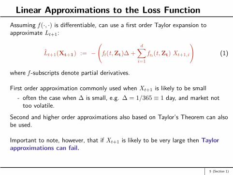
Linear Approximations to the Loss FunctionAssuming f (·, ·) is differentiable, can use a first order Taylor expansion toapproximate Lt+1:

Lt+1(Xt+1) := −

(ft(t,Zt)∆ +

d∑i=1

fzi (t,Zt) Xt+1,i

)(1)

where f -subscripts denote partial derivatives.

First order approximation commonly used when Xt+1 is likely to be small- often the case when ∆ is small, e.g. ∆ = 1/365 ≡ 1 day, and market not

too volatile.

Second and higher order approximations also based on Taylor’s Theorem can alsobe used.

Important to note, however, that if Xt+1 is likely to be very large then Taylorapproximations can fail.

5 (Section 1)

Conditional and Unconditional Loss DistributionsImportant to distinguish between the conditional and unconditional lossdistributions.

Consider the series Xt of risk factor changes and assume that they form astationary time series with stationary distribution FX.

Let Ft denote all information available in the system at time t including inparticular {Xs : s ≤ t}.

Definition: The unconditional loss distribution is the distribution of Lt+1 giventhe time t composition of the portfolio and assuming the CDF of Xt+1 is givenby FX.

Definition: The conditional loss distribution is the distribution of Lt+1 giventhe time t composition of the portfolio and conditional on the information in Ft .

6 (Section 1)

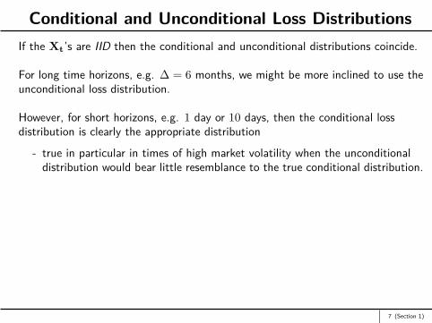
Conditional and Unconditional Loss DistributionsIf the Xt’s are IID then the conditional and unconditional distributions coincide.

For long time horizons, e.g. ∆ = 6 months, we might be more inclined to use theunconditional loss distribution.

However, for short horizons, e.g. 1 day or 10 days, then the conditional lossdistribution is clearly the appropriate distribution

- true in particular in times of high market volatility when the unconditionaldistribution would bear little resemblance to the true conditional distribution.

7 (Section 1)

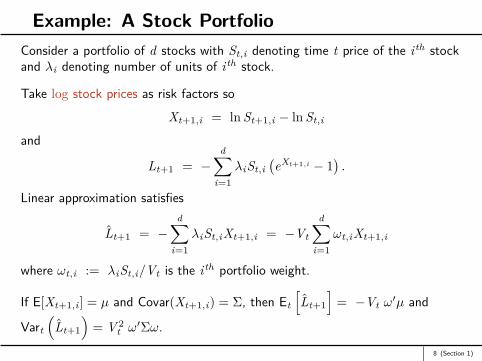
Example: A Stock PortfolioConsider a portfolio of d stocks with St,i denoting time t price of the ith stockand λi denoting number of units of ith stock.

Take log stock prices as risk factors so

Xt+1,i = ln St+1,i − ln St,i

and

Lt+1 = −d∑

i=1λiSt,i

(eXt+1,i − 1

).

Linear approximation satisfies

Lt+1 = −d∑

i=1λiSt,iXt+1,i = −Vt

d∑i=1

ωt,iXt+1,i

where ωt,i := λiSt,i/Vt is the ith portfolio weight.

If E[Xt+1,i ] = µ and Covar(Xt+1,i) = Σ, then Et

[Lt+1

]= −Vt ω

′µ and

Vart

(Lt+1

)= V 2

t ω′Σω.

8 (Section 1)

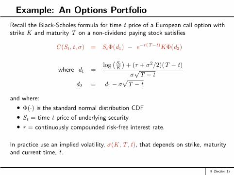
Example: An Options PortfolioRecall the Black-Scholes formula for time t price of a European call option withstrike K and maturity T on a non-dividend paying stock satisfies

C (St , t, σ) = StΦ(d1) − e−r(T−t)KΦ(d2)

where d1 =log(St

K)

+ (r + σ2/2)(T − t)σ√

T − td2 = d1 − σ

√T − t

and where:Φ(·) is the standard normal distribution CDFSt = time t price of underlying securityr = continuously compounded risk-free interest rate.

In practice use an implied volatility, σ(K ,T , t), that depends on strike, maturityand current time, t.

9 (Section 1)

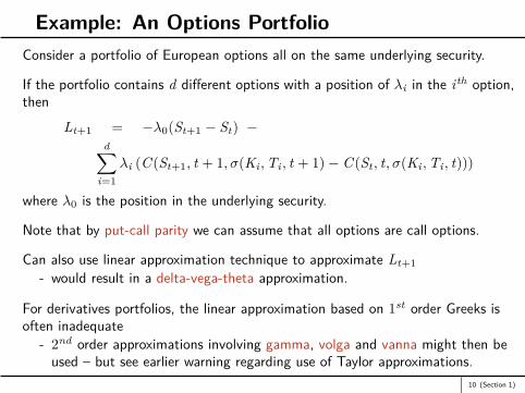
Example: An Options PortfolioConsider a portfolio of European options all on the same underlying security.

If the portfolio contains d different options with a position of λi in the ith option,then

Lt+1 = −λ0(St+1 − St) −d∑

i=1λi (C (St+1, t + 1, σ(Ki ,Ti , t + 1)− C (St , t, σ(Ki ,Ti , t)))

where λ0 is the position in the underlying security.

Note that by put-call parity we can assume that all options are call options.

Can also use linear approximation technique to approximate Lt+1- would result in a delta-vega-theta approximation.

For derivatives portfolios, the linear approximation based on 1st order Greeks isoften inadequate

- 2nd order approximations involving gamma, volga and vanna might then beused – but see earlier warning regarding use of Taylor approximations.

10 (Section 1)

Risk Factors in the Options PortfolioCan again take log stock prices as risk factors but not clear how to handle theimplied volatilities.

There are several possibilities:

1. Assume the σ(K ,T , t)’s simply do not change- not very satisfactory but commonly assumed when historical simulation is

used to approximate the loss distribution and historical data on the changesin implied volatilities are not available.

2. Let each σ(K ,T , t) be a separate factor. Not good for two reasons:(a) It introduces a large number of factors.(b) Implied volatilities are not free to move independently since no-arbitrage

assumption imposes strong restrictions on how volatility surface may move.

Therefore important to choose factors in such a way that no-arbitrage restrictionsare easily imposed when we estimate the loss distribution.

11 (Section 1)

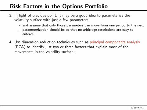
Risk Factors in the Options Portfolio3. In light of previous point, it may be a good idea to parameterize the

volatility surface with just a few parameters- and assume that only those parameters can move from one period to the next- parameterization should be so that no-arbitrage restrictions are easy to

enforce.

4. Use dimension reduction techniques such as principal components analysis(PCA) to identify just two or three factors that explain most of themovements in the volatility surface.

12 (Section 1)

Example: A Bond PortfolioConsider a portfolio containing quantities of d different default-free zero-couponbonds.

Theith bond has price Pt,i , maturity Ti and face value 1.

st,Ti is the continuously compounded spot interest rate for maturity Ti so that

Pt,i = exp(−st,Ti (Ti − t)).

There are λi units of ith bond in the portfolio so total portfolio value given by

Vt =d∑

i=1λi exp(−st,Ti (Ti − t)).

14 (Section 1)

Example: A Bond PortfolioAssume now only parallel changes in the spot rate curve are possible

- while unrealistic, a common assumption in practice- this is the assumption behind the use of duration and convexity.

Then if spot curve moves by δ the portfolio loss satisfies

Lt+1 = −d∑

i=1λi

(e−(st+∆,Ti +δ)(Ti−t−∆) − e−st,Ti (Ti−t)

)' −

d∑i=1

λi (st,Ti (Ti − t) − (st+∆,Ti + δ)(Ti − t −∆)) .

Therefore have a single risk factor, δ.

15 (Section 1)

Approaches to Risk Measurement1. Notional Amount Approach.

2. Factor Sensitivity Measures.

3. Scenario Approach.

4. Measures based on loss distribution, e.g. Value-at-Risk (VaR) or ConditionalValue-at-Risk (CVaR).

16 (Section 2)

An Example of Factor Sensitivity Measures: the Greeks

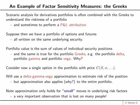
Scenario analysis for derivatives portfolios is often combined with the Greeks tounderstand the riskiness of a portfolio

- and sometimes to perform a P&L attribution.

Suppose then we have a portfolio of options and futures- all written on the same underlying security.

Portfolio value is the sum of values of individual security positions- and the same is true for the portfolio Greeks, e.g. the portfolio delta,

portfolio gamma and portfolio vega. Why?

Consider now a single option in the portfolio with price C (S , σ, . . .).

Will use a delta-gamma-vega approximation to estimate risk of the position- but approximation also applies (why?) to the entire portfolio.

Note approximation only holds for “small” moves in underlying risk factors- a very important observation that is lost on many people!

17 (Section 2)

Delta-Gamma-Vega Approximations to Option Prices

A simple application of Taylor’s Theorem yields

C (S + ∆S , σ + ∆σ) ≈ C (S , σ) + ∆S ∂C∂S + 1

2 (∆S)2 ∂2C∂S2 + ∆σ∂C

∂σ

= C (S , σ) + ∆S δ + 12 (∆S)2 Γ + ∆σ vega.

Therefore obtain

P&L ≈ δ∆S + Γ2 (∆S)2 + vega ∆σ

= delta P&L + gamma P&L + vega P&L .When ∆σ = 0, obtain the well-known delta-gamma approximation

- often used, for example, in historical Value-at-Risk (VaR) calculations.

Can also write

P&L ≈ δS(

∆SS

)+ ΓS2

2

(∆SS

)2+ vega ∆σ

= ESP× Return + $ Gamma× Return2 + vega ∆σ (2)where ESP denotes the equivalent stock position or “dollar” delta.

18 (Section 2)

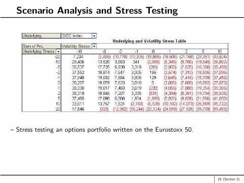
Scenario Analysis and Stress Testing

– Stress testing an options portfolio written on the Eurostoxx 50.

19 (Section 2)

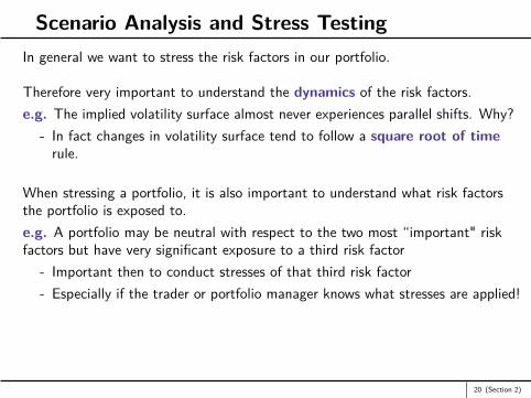
Scenario Analysis and Stress TestingIn general we want to stress the risk factors in our portfolio.

Therefore very important to understand the dynamics of the risk factors.e.g. The implied volatility surface almost never experiences parallel shifts. Why?

- In fact changes in volatility surface tend to follow a square root of timerule.

When stressing a portfolio, it is also important to understand what risk factorsthe portfolio is exposed to.e.g. A portfolio may be neutral with respect to the two most “important" riskfactors but have very significant exposure to a third risk factor

- Important then to conduct stresses of that third risk factor- Especially if the trader or portfolio manager knows what stresses are applied!

20 (Section 2)

Value-at-RiskValue-at-Risk (VaR) the most widely (mis-)used risk measure in the financialindustry.

Despite the many weaknesses of VaR, financial institutions are required to use itunder the Basel II capital-adequacy framework.

And many institutions routinely report VaR numbers to shareholders, investors orregulatory authorities.

VaR is calculated from the loss distribution

- could be conditional or unconditional- could be a true loss distribution or some approximation to it.

Will assume that horizon ∆ has been fixed so that L represents portfolio lossover time interval ∆.

Will use FL(·) to denote the CDF of L.

22 (Section 2)

Value-at-RiskDefinition: Let F : R→ [0, 1] be an arbitrary CDF. Then for α ∈ (0, 1) theα-quantile of F is defined by

qα(F) := inf{x ∈ R : F(x) ≥ α}.

If F is continuous and strictly increasing, then qα(F) = F−1(α).For a random variable L with CDF FL(·), will often write qα(L) instead ofqα(FL).Since any CDF is by definition right-continuous, immediately obtain thefollowing result:

Lemma: A point x0 ∈ R is the α-quantile of FL if and only if

(i) FL(x0) ≥ α and(ii) FL(x) < α for all x < x0.

Definition: Let α ∈ (0, 1) be some fixed confidence level. Then the VaR of theportfolio loss at the confidence interval, α, is given by VaRα := qα(L), theα-quantile of the loss distribution.

23 (Section 2)

VaR for the Normal DistributionsBecause the normal CDF is both continuous and strictly increasing, it isstraightforward to calculate VaRα.

So suppose L ∼ N(µ, σ2). Then

VaRα = µ+ σΦ−1(α) (3)

where Φ(·) is the standard normal CDF.

This follows from previous lemma if we can show FL(VaRα) = α

- but this follows immediately from (3).

24 (Section 2)

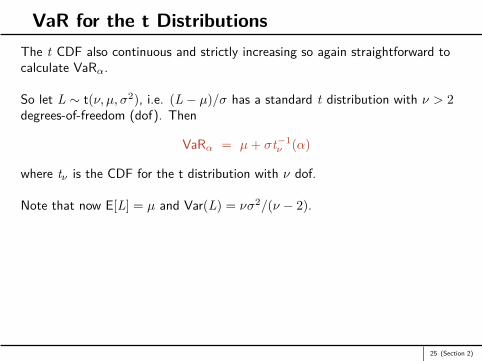
VaR for the t DistributionsThe t CDF also continuous and strictly increasing so again straightforward tocalculate VaRα.

So let L ∼ t(ν, µ, σ2), i.e. (L − µ)/σ has a standard t distribution with ν > 2degrees-of-freedom (dof). Then

VaRα = µ+ σt−1ν (α)

where tν is the CDF for the t distribution with ν dof.

Note that now E[L] = µ and Var(L) = νσ2/(ν − 2).

25 (Section 2)

Weaknesses of VaR1. VaR attempts to describe the entire loss distribution with just a single

number!- so significant information is lost- this criticism applies to all scalar risk measures- one way around it is to report VaRα for several values of α.

2. Significant model risk attached to VaR- e.g. if loss distribution is heavy-tailed but a light-tailed, e.g. normal,

distribution is assumed, then VaRα will be severely underestimated as α → 1.

3. A fundamental problem with VaR is that it can be very difficult to estimatethe loss distribution

- true of all risk measures based on the loss distribution.

4. VaR is not a sub-additive risk measure so that it doesn’t lend itself toaggregation.

26 (Section 2)

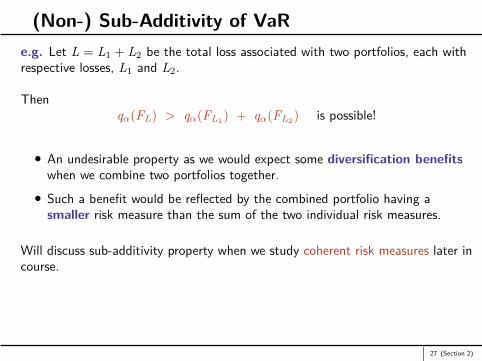
(Non-) Sub-Additivity of VaRe.g. Let L = L1 + L2 be the total loss associated with two portfolios, each withrespective losses, L1 and L2.

Thenqα(FL) > qα(FL1) + qα(FL2) is possible!

An undesirable property as we would expect some diversification benefitswhen we combine two portfolios together.

Such a benefit would be reflected by the combined portfolio having asmaller risk measure than the sum of the two individual risk measures.

Will discuss sub-additivity property when we study coherent risk measures later incourse.

27 (Section 2)

Advantages of VaRVaR is generally “easier” to estimate:

True of quantile estimation in general since quantiles are not very sensitiveto outliers.

- not true of other risk measures such as Expected Shortfall / CVaREven then, it becomes progressively more difficult to estimate VaRα asα→ 1

- may be able to use Extreme Value Theory (EVT) in these circumstances.

But VaR easier to estimate only if we have correctly specified the appropriateprobability model

- often an unjustifiable assumption!

Value of ∆ that is used in practice generally depends on the application:For credit, operational and insurance risk ∆ often on the order of 1 year.For financial risks typical values of ∆ are on the order of days.

28 (Section 2)

Expected Shortfall (ES)Definition: For a portfolio loss, L, satisfying E[|L|] <∞ the expected shortfallat confidence level α ∈ (0, 1) is given by

ESα := 11− α

∫ 1

α

qu(FL) du. (4)

Relationship between ESα and VaRα is therefore given by

ESα := 11− α

∫ 1

α

VaRu(L) du

- so clear that ESα(L) ≥ VaRα(L).

29 (Section 2)

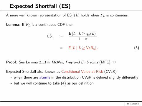
Expected Shortfall (ES)A more well known representation of ESα(L) holds when FL is continuous:

Lemma: If FL is a continuous CDF then

ESα := E [L; L ≥ qα(L)]1− α

= E [L | L ≥ VaRα] . (5)

Proof: See Lemma 2.13 in McNeil, Frey and Embrechts (MFE). 2

Expected Shortfall also known as Conditional Value-at-Risk (CVaR)- when there are atoms in the distribution CVaR is defined slightly differently- but we will continue to take (4) as our definition.

30 (Section 2)

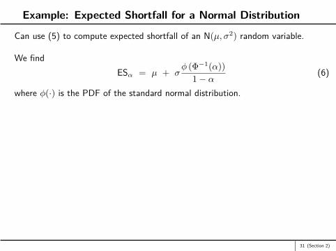
Example: Expected Shortfall for a Normal Distribution

Can use (5) to compute expected shortfall of an N(µ, σ2) random variable.

We findESα = µ + σ

φ (Φ−1(α))1− α (6)

where φ(·) is the PDF of the standard normal distribution.

31 (Section 2)

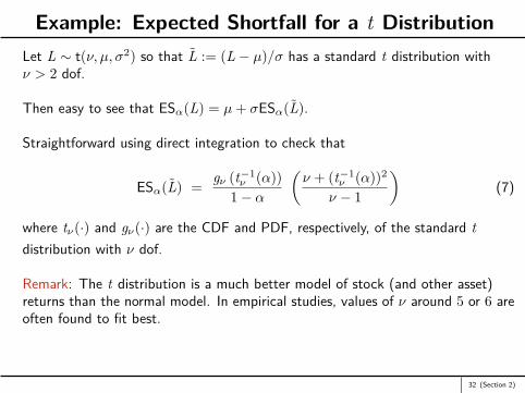
Example: Expected Shortfall for a t DistributionLet L ∼ t(ν, µ, σ2) so that L := (L − µ)/σ has a standard t distribution withν > 2 dof.

Then easy to see that ESα(L) = µ+ σESα(L).

Straightforward using direct integration to check that

ESα(L) = gν (t−1ν (α))

1− α

(ν + (t−1

ν (α))2

ν − 1

)(7)

where tν(·) and gν(·) are the CDF and PDF, respectively, of the standard tdistribution with ν dof.

Remark: The t distribution is a much better model of stock (and other asset)returns than the normal model. In empirical studies, values of ν around 5 or 6 areoften found to fit best.

32 (Section 2)

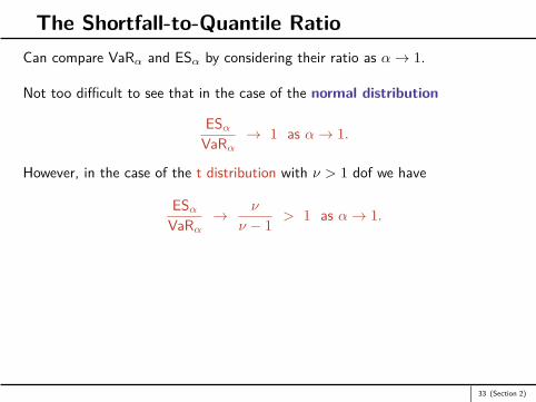
The Shortfall-to-Quantile RatioCan compare VaRα and ESα by considering their ratio as α→ 1.

Not too difficult to see that in the case of the normal distribution

ESαVaRα

→ 1 as α→ 1.

However, in the case of the t distribution with ν > 1 dof we have

ESαVaRα

→ ν

ν − 1 > 1 as α→ 1.

33 (Section 2)

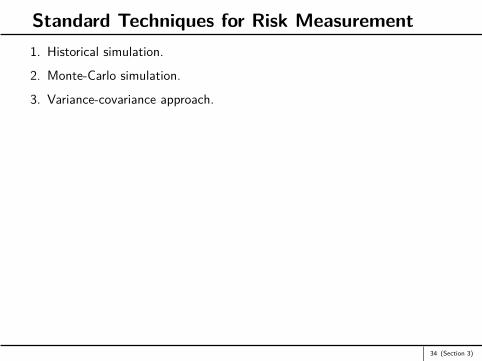
Standard Techniques for Risk Measurement1. Historical simulation.

2. Monte-Carlo simulation.

3. Variance-covariance approach.

34 (Section 3)

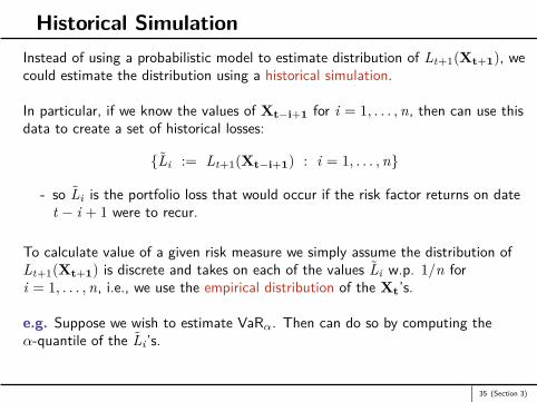
Historical SimulationInstead of using a probabilistic model to estimate distribution of Lt+1(Xt+1), wecould estimate the distribution using a historical simulation.

In particular, if we know the values of Xt−i+1 for i = 1, . . . ,n, then can use thisdata to create a set of historical losses:

{Li := Lt+1(Xt−i+1) : i = 1, . . . ,n}

- so Li is the portfolio loss that would occur if the risk factor returns on datet − i + 1 were to recur.

To calculate value of a given risk measure we simply assume the distribution ofLt+1(Xt+1) is discrete and takes on each of the values Li w.p. 1/n fori = 1, . . . ,n, i.e., we use the empirical distribution of the Xt’s.

e.g. Suppose we wish to estimate VaRα. Then can do so by computing theα-quantile of the Li ’s.

35 (Section 3)

Historical SimulationSuppose the Li ’s are ordered by

Ln,n ≤ · · · ≤ L1,n.

Then an estimator of VaRα(Lt+1) is L[n(1−α)],n where [n(1− α)] is the largestinteger not exceeding n(1− α).

Can estimate ESα using

ESα =L[n(1−α)],n + · · · + L1,n

[n(1− α)] .

Historical simulation approach generally difficult to apply for derivative portfolios.Why?But if applicable, then easy to apply.

Historical simulation estimates the unconditional loss distribution- so not good for financial applications!

36 (Section 3)

Monte-Carlo SimulationMonte-Carlo approach similar to historical simulation approach.

But now use some parametric distribution for the change in risk factors togenerate sample portfolio losses.

The (conditional or unconditional) distribution of the risk factors is estimatedand m portfolio loss samples are generated.

Free to make m as large as possibleSubject to constraints on computational time.Variance reduction methods often employed to obtain improved estimates ofrequired risk measures.

While Monte-Carlo is an excellent tool, it is only as good as the model used togenerate the data: if the estimated distribution of Xt+1 is poor, thenMonte-Carlo of little value.

37 (Section 3)

The Variance-Covariance ApproachIn the variance-covariance approach assume that Xt+1 has a multivariate normaldistribution so that

Xt+1 ∼ MVN (µ,Σ) .

Also assume the linear approximation

Lt+1(Xt+1) := −

(ft(t,Zt)∆ +

d∑i=1

fzi (t,Zt) Xt+1,i

)

is sufficiently accurate. Then can write

Lt+1(Xt+1) = −(ct + bt>Xt+1)

for a constant scalar, ct , and constant vector, bt.

Therefore obtain

Lt+1(Xt+1) ∼ N(−ct − bt

>µ, bt>Σbt

).

and can calculate any risk measures of interest.38 (Section 3)

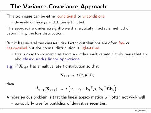
The Variance-Covariance ApproachThis technique can be either conditional or unconditional

- depends on how µ and Σ are estimated.The approach provides straightforward analytically tractable method ofdetermining the loss distribution.

But it has several weaknesses: risk factor distributions are often fat- orheavy-tailed but the normal distribution is light-tailed

- this is easy to overcome as there are other multivariate distributions that arealso closed under linear operations.

e.g. If Xt+1 has a multivariate t distribution so that

Xt+1 ∼ t (ν,µ,Σ)

thenLt+1(Xt+1) ∼ t

(ν,−ct − bt

>µ, bt>Σbt

).

A more serious problem is that the linear approximation will often not work well- particularly true for portfolios of derivative securities.

39 (Section 3)

Evaluating Risk Measurement TechniquesImportant for any risk manger to constantly evaluate the reported risk measures.

e.g. If daily 95% VaR is reported then should see daily losses exceeding thereported VaR approximately 95% of the time.

So suppose reported VaR numbers are correct and define

Yi :={

1, Li ≥ VaRi0, otherwise

where VaRi and Li are the reported VaR and realized loss for period i.

If Yi ’s are IID, thenn∑

i=1Yi ∼ Binomial(n, .05)

Can use standard statistical tests to see if this is indeed the case.

Similar tests can be constructed for ES and other risk measures.

40 (Section 3)

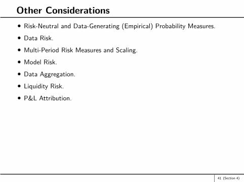
Other ConsiderationsRisk-Neutral and Data-Generating (Empirical) Probability Measures.

Data Risk.

Multi-Period Risk Measures and Scaling.

Model Risk.

Data Aggregation.

Liquidity Risk.

P&L Attribution.

41 (Section 4)