if anything is unclear, please ask ! - international ... · Ædoes not cover people deciding to...

SUMMMARY

O

T i i

OFTRA

IN

Training summary

• Employment analysis: Concepts, instruments, NING

p y y papplications

• Labour market information systems

l j i h d d li i• Employment projections: Methods and an application

If anything is unclear, please ask !

EMPLOYMENT ANALYSIS: CONCEPTS, INSTRUMENTSEkkehard ERNST

Port of Spain, Nov 2nd 2011

Ekkehard ERNST

OVERV

IEW

O iOverview

• Concepts for labour market analysisp y

• Measuring the labour market

• Labour market analysis: Approaches

• Labour market analysis: Models

• Labour market analysis: Policies

TRA

IININGOB

T i i bj ti

BJECTIVE

Training objectives

• Get an overview of commonly used employment ESy p yindicators

• Understanding broad trends

d i i l i i• Introduction in analysis instruments…

• …and application to current problems

LABOUR MARKET ANALYSIS: CONCEPTS

LABO

Labour market analysis: Some basicsOURMA

• Observed employment is the result of several,

decentralised decisions RKETCO

decentralised decisionsParticipating in the labour market

Finding gainful employment ONCEPTS

Deciding how many hours to work

• In technical language we write:

( )( ) LFURHOURSETF ×−×= 1• Notation:Notation:

ETF: Total employment (full‐time equivalent)

HOURS: Hours worked per person

UR: Unemployment rate

LF: Labour force

LABO

Labour forceOURMA

• The labour force is constituted by all those who are contributing to productive employment RKET

CO

co t but g to p oduct e e p oy e tCovers both employed and job seekers

Does not cover people deciding to stay or become inactive...

h i bl t t k l t ( th

ONCEPTS

...or who are incapable to take up employment (e.g. those

with health problems)

Typically covers people above age 15.

• Inactivity can be a choice:Taxes are too high for second earners (women) to seek for

employmentemployment

Social assistance is too generous

Opportunity costs are too high (in comparison to the wage

that can be earned)

LABO

EmploymentOURMA

• Employment counts from the first hour...Employment does not indicate the number of hours worked RKET

CO

...nor the type of work carried out.

It is only a numeric head‐count indicator of all those who

contribute to a country’s productive capacity

ONCEPTS

contribute to a country s productive capacity

• Without employment covers different statuses:Job seekers, i.e. Who would like to work but can’t find

employment

Inactive, i.e. who do not or cannot work (physically or

mentally weak people)mentally weak people)

Those who would like to work but have given up to search,

i.e. discouraged workers

LABO

Types of employmentOURMA

• Several forms of employment...Dependent employment (wage earners) RKET

CO

Dependent employment (wage earners)

Self‐employment (independent workers)

Own account workers (e.g. entrepreneurs)

I f l l t ( ith t l b t t)

ONCEPTS

Informal employment (e.g. without proper labour contract)

Temporary employment

• not all of which work full time:• ... not all of which work full time:Full‐time employees (regularly work more than 30 hours per

week)

Part‐time employees (regularly work less than 30 hours per

week, sometimes very few hours: even 1 hour counts !)...

...which sometimes is involuntaryy

LABO

Working hoursOURMA

• Different aspects of working timeNormal working hours RKET

CO

Normal working hours

Over‐time working hours

Regular working hours ONCEPTS

• For labour market analysis only regular working

hours are relevantProductive capacity increases with every hour, whether it

is overtime or not

Regulation of overtime constitutes, however, important

incentives for employers wrt expansion of workforce

The marginal productivity may decline as average

working hours increaseworking hours increase...

...but the average productivity (per worker) increases in

any case

LABO

UnemploymentOURMA

• Unemployment concerns all those without a job who:Have not been working over the last week/month, not even RKET

CO

for an hour...

...are looking for a job...

and ready to take up an occupation immediately (i e no

ONCEPTS

...and ready to take up an occupation immediately (i.e. no

health problems, child care issues, etc.)

• Some job seekers are unemployed for longer spells:Typically unemployment spells above 6 months are

considered to be long‐term

People tend to loose skills (both technical and non‐technical,People tend to loose skills (both technical and non technical,

“soft” skills)

LTU are more difficult to mobilise and activate to return to

l temployment

LABO

Labour market flows IOURMA

• Most labour market surveys only cover “stocks”Current situation of interviewed person in the labour RKET

CO

Current situation of interviewed person in the labour

market

No regard to dynamic aspects: “What have you be doing

1 th/ t / ?”

ONCEPTS

1 month/quarter/year ago?”

• Labour market theory makes use of flowsThe extent to which employment is created depends onThe extent to which employment is created depends on

how difficult it is for an employer to find new workers

It also depends on his/her expectations regarding future

developments

Finally, it also depends on wage earners expectations and

salary requirementsy q

LABO

Labour market flows IIOURMA

• Labour market analysis needs more informationEffects of policies depend on the speed of flows more RKET

CO

Effects of policies depend on the speed of flows more

than on the impact of stocks

Additional sources of information can be used but are

t it h l f l l d i d l b f

ONCEPTS

not quite as helpful as properly designed labour force

surveys

• Some proxy indicators• Some proxy indicatorsVacancy information, help‐wanted‐index, online ads

Unemployment duration and probabilities of finding new

employment

LABOUR MARKET ANALYSIS: MEASUREMENT

MEA

Employment trends across countries…ASU

RING80

Employment‐to‐population ratios (2007 vs. 2010)

THELA

B

ISL

IDN

KAZ

NZL

NOR

PERRUS

SWE

THA

70

BOURM

AUS

AUT

BEL

BRA

CAN

CHL

CHN

COL

CYP

CZE

DNK

EST

FIN

FRA

DEU

IDN

IRLISR

JPNKOR

LUXMUS

NLD

PHL

POL

PRT

ROM

RUS

SVK

TWN

UKR

GBRUSAVEN

060

2010

ARKET

BEL

BUL

HRV

EST

GRCHUNITA

LVALTU

MKD

MLT

MDA

POL

SLV

ZFA

ESP

TUR

4050

MAR

30

30 40 50 60 70 802007

MEA

Employment to population ratiosASU

RINGTH

ELA

BWPOPETEPR =

BOURM

WPOP

l l

ARKET

•ET: Total employment

•WPOP: Working‐age population, i.e. all people 15 years and aboveand above

EPR: Employment‐to‐population ratio

MEA

Employment index ‐ CalculationsASU

RING

• Take a particular date as base year, e.g. 2005Take a particular date as base year, e.g. 2005 TH

ELA

B

Take a particular date as base year, e.g. 2005

Calculate the relative level of following years with

respect to that base year

BOURM

BaseYear

tBaseYeart ET

ETIndexET +×=− 100

ARKET

• Some words of cautionWhen grouping countries, add the absolute employment

BaseYear

levels first before constructing the index

Try to find a base year with a particular meaning (e.g.

peak of the cycle)p y )

MEA

…and at the regional level: Global shifts in employmentASU

RING

Employment developments (index, 2005=100)

THELA

BBOURMARKET

MEA

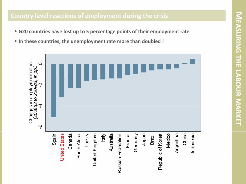
Country level reactions of employment during the crisisASU

RING

• G20 countries have lost up to 5 percentage points of their employment rate

• In these countries, the unemployment rate more than doubled !

THELA

B

0

ent r

ates

in p

p.)

BOURM

4-2

in e

mpl

oym

eq3

to 2

009q

3,

ARKET

-6-4

Cha

nges

(2

008q

Spai

n

nite

d S

tate

s

Can

ada

Sout

h Af

rica

Turk

ey

ed K

ingd

om Italy

Aust

ralia

n Fe

dera

tion

Fran

ce

Ger

man

y

Japa

n

Braz

il

blic

of K

orea

Mex

ico

Arge

ntin

a

Chi

na

Indo

nesi

a

U S

Uni

t

Russ

ian

Rep

ub

MEA

Temporary employment took the largest hitASU

RING

Temporary employment in the EU (%‐change year‐on‐year)

THELA

BBOURMARKET

MEA

Employment adjustment: Hours‐Job count mix differs across countriesASU

RINGTH

ELA

BBOURMARKET

MEA

Sectoral developments…ASU

RINGTH

ELA

BBOURMARKET

MEA

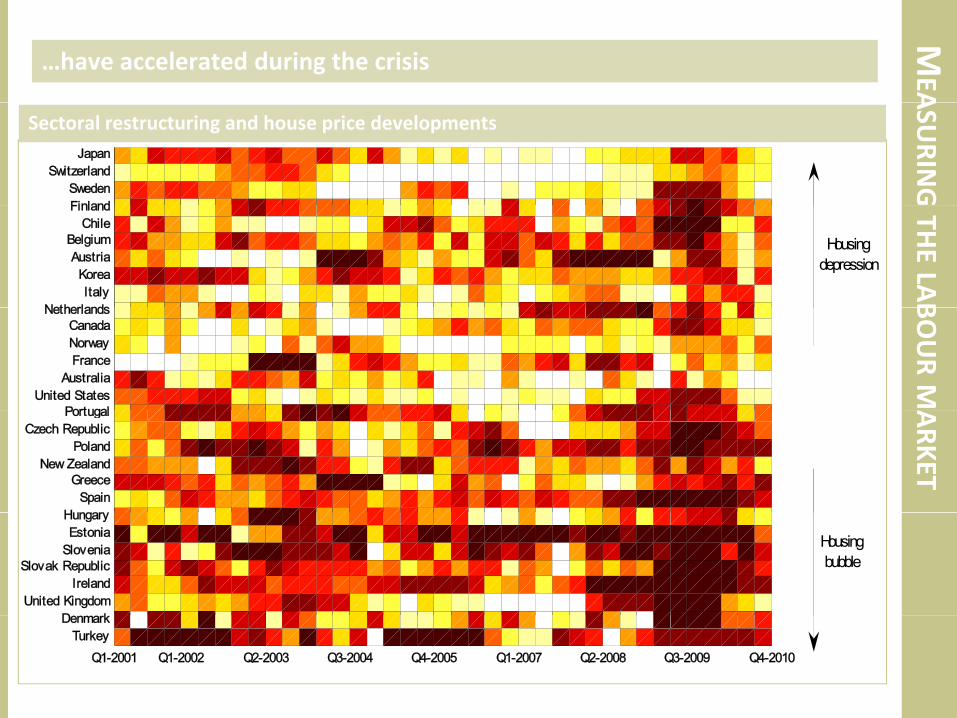
…have accelerated during the crisisASU

RING

FinlandSweden

SwitzerlandJapan

Sectoral restructuring and house price developments

THELA

B

NetherlandsItaly

KoreaAustria

BelgiumChile

Finland

Housingdepression

BOURM

PortugalUnited States

AustraliaFranceNorwayCanada

Netherlands

ARKET

HungarySpain

GreeceNew Zealand

PolandCzech Republic

Portugal

D kUnited Kingdom

IrelandSlovak Republic

SloveniaEstonia

Hungary

Housingbubble

Q1-2001 Q1-2002 Q2-2003 Q3-2004 Q4-2005 Q1-2007 Q2-2008 Q3-2009 Q4-2010

TurkeyDenmark

MEA

Sectoral adjustmentASU

RING

• How to calculate the intensity of employment reallocation

across sectors?Si l l l i di TH

ELA

B

Simple to calculate indicator

Only one number

Most commonly used: Lilien indicator BOURM( )

2/1

1loglog ⎥

⎦

⎤⎢⎣

⎡∑ Δ−Δ=J

jt

djt

djt EEEE

Lilien

ARKET

1 ⎦⎣ =j tE• where j: sector, J: number of sectors, t: year/quarter/month, d:

i i d hi h l dj i id d (1 5time period over which sectoral adjustment is considered (1 year, 5

years, 1 quarter, etc.)

• The indicator will change depending on:the sectoral detail (number of sectors J)

the period over which change is considered (i.e. d)

MEA

Unemployment developments,ASU

RING

200

Evolution of unemployment (2005‐2010, 2005q4 = 100)

THELA

B

150

BOURM

100

ARKET50

Western Europe Eastern Europe and CIS

Southern Europe North America and Oceania

Asia Latin America

MEA

…long‐term unemployment, …ASU

RING180

Percentage increase in numbers of long‐term unemployed, Q1 2009–Q1 2010

THELA

B90

120

150

BOURM

0

30

60

ARKET

‐30

0

huania

nmark

stonia

reland

Cyprus

Latvia

States

Spain

orway

Finland

weden

ngdom

ovakia

ortugal

ulgaria

epublic

ovenia

Greece

Turkey

France

ungary

Italy

Japan

rlands

elgium

Poland

Malta

Brazil

mbourg

Africa

Austria

omania

rmany

ia, FYR

Croatia

Lith

De E I C

United N F Sw

United Kin Slo

Po BuCzech Re Slo G T F

Hu

Nethe Be P

Luxem

South ARo Ge

Macedoni C

MEA

…and inactivity increased during the crisis...ASU

RING

Inactive population (in % of working‐age‐population)

THELA

BBOURMARKET

MEA

…against the background of large scale under‐employmentASU

RINGTime‐related under‐employment (in % of labour force), latest year available

THELA

B

20.0

25.0

BOURM

10.0

15.0

ARKET

0 0

5.0

0.0

MEA

Youth unemployment has acceleratedASU

RINGTH

ELA

BBOURMARKET

MEA

Youth unemployment by regionASU

RINGTH

ELA

BBOURMARKET

MEA

Unemployment flows IASU

RING

Unemployment in‐ and outflows in US, Canada, Japan and UK

35% 2.5%

THELA

B

30%

Outflow

BOURM25% 2.0%

ARKET20%

Inflow

15%

1987

1988

1989

1990

1991

1992

1993

1994

1995

1996

1997

1998

1999

2000

2001

2002

2003

2004

2005

2006

2007

2008

2009

*

1.5%

Inflow

MEA

Unemployment flows IIASU

RING

9% 0 8%

Unemployment in‐ and outflows in France, Germany and Italy

THELA

B

9% 0.8%

BOURM

7%

0.6%

Outflow

ARKET

5%

Inflow

4%

1987

1988

1989

1990

1991

1992

1993

1994

1995

1996

1997

1998

1999

2000

2001

2002

2003

2004

2005

2006

2007

2008

2009

*

0.4%

EMPLOYMENT ANALYSIS

EMP

Questions for employment analysisPLO

YMEN

• How to stimulate employmentIs employment growing in line with output/productivity?

Are certain categories benefiting more/less from output

NTANALY

Are certain categories benefiting more/less from output

growth?

Which sectors contribute to employment most?

YSIS• How to improve income generationCan wages increase without creating unemployment?

Do policies need to adjust to stimulate/restrict wage growth?p j / g g

Is the economy gaining/loosing competitiveness?

• How to enhance labour market chancesCan workers switch easily between jobs/firms/sectors?

Do job seekers find quickly re‐employment?

How do policies need to adjust to stimulate labour market

reactivity

EMP

How to analyse employment developmentsPLO

YMEN

• Three levels of analysisOver the medium run: Link between employment and

h/ d i i

NTANALY

growth/productivity

Over the short run: Trade‐off between higher wages and

lower unemployment YSISDynamic analysis: Understanding labour market flows

• The (appropriate) level of analysis depends on the availability of data:

Key Indicators of the Labour Market: Contains

information on employment and growth for all 182 ILOinformation on employment and growth for all 182 ILO

member countries

KILM also has information for wages but with less

coverage

So far only limited information available for flows

EMP

Medium‐run analysis: The Okun’s curve IPLO

YMEN

• Traditional approach to labour market analysis:Statistical relationship between output growth and N

TANALY

Statistical relationship between output growth and

unemployment

Alternative: Elasticity between growth and employment

All t i htf d l l ti f l t

YSIS: OK

Allows straightforward calculation of employment

developments once GDP estimates have been carried out

KUN’S

CUURV

E

EMP

Medium‐run analysis: The Okun’s curve IIPLO

YMEN

• Underlying approach to the GET (Global employment

Trends) NTANALY

e ds)

• Comes in two varietiesIdentify different elasticities depending on whether we are in YSIS: O

K

a recession or a boom

OR: Use historical elasticities

• Bottom‐up approach: Use sectoral elasticities and KUN’S

CU

Bottom up approach: Use sectoral elasticities and

aggregate

• Based on annual data URV

E

EMP

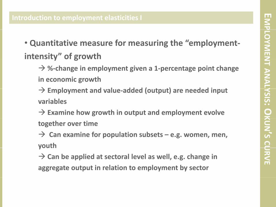
Introduction to employment elasticities IPLO

YMEN

• Quantitative measure for measuring the “employment‐

intensity” of growth NTANALY

te s ty o g o t%‐change in employment given a 1‐percentage point change

in economic growth

E l t d l dd d ( t t) d d i t

YSIS: OK

Employment and value‐added (output) are needed input

variables

Examine how growth in output and employment evolve KUN’S

CU

together over time

Can examine for population subsets – e.g. women, men,

youth URV

E

youth

Can be applied at sectoral level as well, e.g. change in

aggregate output in relation to employment by sector

EMP

Introduction to employment elasticities IIPLO

YMEN

• When value‐added and employment data correspond

to precisely the same group: NTANALY

to p ec se y t e sa e g oup:%‐change in labour productivity given a 1‐percentage point

change in economic growth

S t d i d t l l t d i

YSIS: OK

Sector and industry‐level trends in an economy

•Analysing structural changes in employment: KUN’S

CU

Movement from agriculture to higher value added sectors

Labour absorbing versus labour shedding industries

URV

E

EMP

Calculating employment elasticitiesPLO

YMEN

• Two main methods:“Arc”‐elasticity (spreadsheet calculation): N

TANALY

( )( ) =

−⎛⎝⎜

⎞⎠⎟

εii i iE E E

Y Y Y1 0 0/

/ YSIS: OK“Point”‐elasticity (using econometric regressions):

( )−⎝ ⎠i i iY Y Y1 0 0/

KUN’S

CU

YE lnln βα +=1:

URV

E

2: ββ =⎟⎠⎞

⎜⎝⎛

∂∂

→⎟⎠⎞

⎜⎝⎛ ∂

=∂

EY

YE

YY

EE

⎠⎝∂⎠⎝ EYYE

EMP

Which method should I use?PLO

YMEN

• The “arc” method is preferred when there are very few

data (e.g. year‐over year comparison): NTANALY

data (e.g. yea o e yea co pa so ):Computationally simple (can be worked out by hand or in a

spreadsheet)

L d t l til lt

YSIS: OK

Leads to volatile results

• The “point” method is preferred when there are KUN’S

CU

several observations:Provides more stable results

Gi l i hi b h i bl h

URV

E

Gives average relationship between the variables over the

period in question, instead of relationship between start‐ and

end‐points

EMP

Relationship between elasticities, productivity and employmentPLO

YMEN

• When output and employment correspond to the same

group, there is a special relationship: NTANALY

g oup, t e e s a spec a e at o s p:

Y = E Pi i i× YSIS: OKΔ Δ ΔY = E Pi i i+ KU

N’SCU

where ∆ represents the growth rate of a particular variable

•We then have: URV

E

We then have:

ε = 1 − Δ P

ε =Δ E

ε = 1 Δ Y

ε =Δ Y

EMP

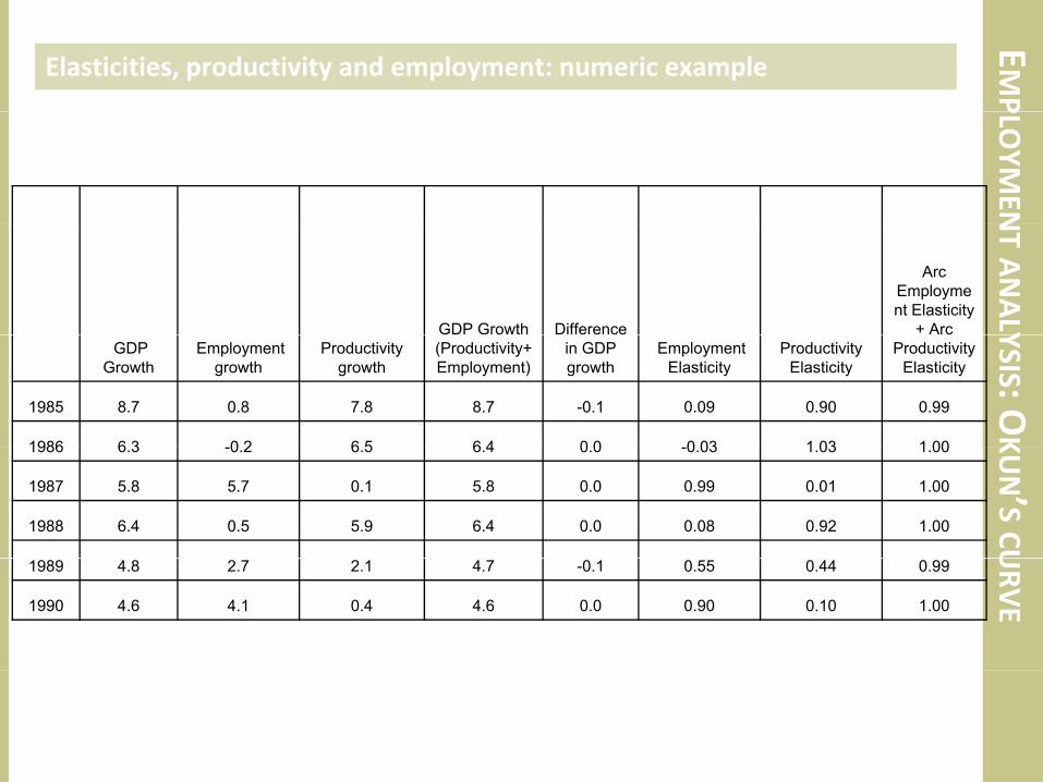
Elasticities, productivity and employment: numeric examplePLO

YMENN

TANALYGDP Growth Difference

Arc Employment Elasticity

+ Arc YSIS: OK

GDP Growth

Employment growth

Productivity growth

(Productivity+Employment)

in GDP growth

Employment Elasticity

Productivity Elasticity

Productivity Elasticity

1985 8.7 0.8 7.8 8.7 -0.1 0.09 0.90 0.99

1986 6 3 0 2 6 5 6 4 0 0 0 03 1 03 1 00

KUN’S

CU

1986 6.3 -0.2 6.5 6.4 0.0 -0.03 1.03 1.00

1987 5.8 5.7 0.1 5.8 0.0 0.99 0.01 1.00

1988 6.4 0.5 5.9 6.4 0.0 0.08 0.92 1.00 URV

E

1989 4.8 2.7 2.1 4.7 -0.1 0.55 0.44 0.99

1990 4.6 4.1 0.4 4.6 0.0 0.90 0.10 1.00

EMP

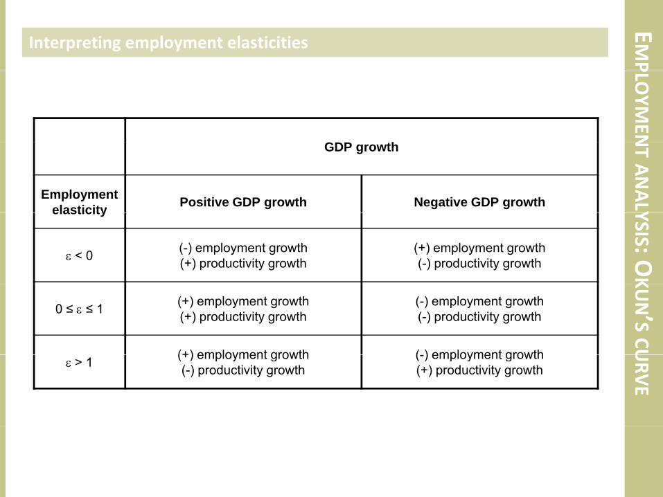
Interpreting employment elasticitiesPLO

YMEN

G

NTANALY

GDP growth

Employmentelasticity Positive GDP growth Negative GDP growth YSIS: O

K

elasticity

ε < 0 (-) employment growth(+) productivity growth

(+) employment growth(-) productivity growth KU

N’SCU

0 ≤ ε ≤ 1 (+) employment growth(+) productivity growth

(-) employment growth(-) productivity growth

(+) employment growth ( ) employment growth

URV

E

ε > 1 (+) employment growth(-) productivity growth

(-) employment growth(+) productivity growth

EMP

Employment may be more elastic even with lower GDP growthPLO

YMEN

Employment elasticities versus GDP growth in Asia (200‐2004)

9

10

NTANALY7

8

9

%)

China

Vietnam YSIS: OK5

6

ual G

DP g

row

th (%

India

BangladeshThailand

K

KUN’S

CU3

4

Aver

age

annu

Sri Lanka

Singapore

Malaysia PhilippinesPakistanKorea

Indonesia

URV

E

1

2

00 0.1 0.2 0.3 0.4 0.5 0.6 0.7 0.8

Employment elasticity

EMP

Sectoral elasticities in Pakistan, 1992‐2004 PLO

YMEN

Agriculture Value Added

Industry Value Added

Services Value Added

NTANALY

Agriculture Industry Services

Added Growth

(average annual %)

Added Growth

(average annual %)

Added Growth

(average annual %)

YSIS: OK

Pakistan 0.19 1.31 1.18 2.8 4.3 4.3

• With sufficient sectoral information elasticities can be

KUN’S

CU

• With sufficient sectoral information, elasticities can be

split:Information on employment elasticity by sector U

RVEBut: No information about cross elasticities:

“How much employment in sector 1 is modified with a 1%‐

change in value added in sector 2”change in value added in sector 2

EMP

Main characteristics of Okun‘s elasticitiesPLO

YMEN

• Backward‐looking• Dynamic N

TANALY

y a c

• Volatile• No “ideal” figure YSIS: O

K

• Misleading when used in isolation

• Complementary when used with GDP growth, KUN’S

CU

unemployment rates and other LMI

URV

E

EMP

Problems with the Okun’s curvePLO

YMEN

• Problems:Non‐stable relationship: Intensity of job creation varies over N

TANALY

the business cycle

Non‐stable relationship II: Intensity of job creation changes

with sectoral adjustment YSIS: OK

with sectoral adjustment

Problems of statistical identification: Growth‐employment

elasticity differs depending on the time horizon at which to KUN’S

CU

look What is the right horizon?

URV

E

EMP

Applying the Okun‘s curve to current problems: G20PLO

YMEN

• Estimating employment elasticities using the “Point”‐

elasticity:

NTANALY

elasticity:Problem: Often time series are very short, especially for

employment YSIS: OK

Missing data

• Solution: KUN’S

CU

Using panel data

Group data from different countries

Calculate panel‐wide elasticity on a larger sample URV

E

EMP


YMEN

• But:How to take into account differences across countries? N

TANALY

How to take into account differences across countries?

Are the country elasticities the same ?

• Solution: YSIS: OK

Use fixed effects for level differences across countries

Differentiate coefficients across countries

Group data to improve efficiency of estimation

KUN’S

CU

Group data to improve efficiency of estimation

GDPET β

URV

Eititiiit GDPET εβα ++=

EMP


YMEN

Country Country‐specific coefficient

Argentina 0.31 NTANALY

Australia 0.57Brazil 0.23Canada 0.57China 0.02F 0 35

YSIS: OK

France 0.35Germany 0.29India 0.04Indonesia 0.12Italy 0.31 KU

N’SCU

yJapan 0.28Korea 0.34Mexico 0.13Russia 0.32 U

RVE

Saudi Arabia 0.24South Africa 0.77Spain 1.18Turkey 0.32United Kingdom 0 47United Kingdom 0.47USA 0.59

EMP


YMENN

TANALYYSIS: O

KKUN’S

CUURV

E

EMP

Applying the Okun‘s curve to current problems: Fiscal multiplier IPLO

YMEN

• Okun’s elasticities can also be used for policy analysis:How much employment can be generated from a 1%‐ N

TANALY

How much employment can be generated from a 1%

increase in public spending

How should public spending and taxation evolve over the

b i l ? P /A /C t li l?

YSIS: OK

business cycle? Pro‐/A‐/Counter‐cyclical?

• Extended Okun’s curve estimation:Add an estimate of the impact of public spending/deficit on

KUN’S

CU

Add an estimate of the impact of public spending/deficit on

GDP to the employment elasticity

1

URV

E

2

1ititiiit

diP bli SGDP

GDPET

δ

εβα

++

++=2ititiiit dingPublicSpenGDP εδγ ++=

EMP

Applying the Okun‘s curve to current problems: Fiscal multiplier IIPLO

YMEN1.4

1.6

1.8

2.0

ultip

liers

Emerging economies

NTANALY0.4

0.6

0.8

1.0

1.2

Em

ploy

men

t mu

YSIS: OK

1.61.82.0

rs

Advanced economies0.0

0.2

Arge

ntin

a

Sout

hAfri

ca

Mex

ico

Bots

wan

a

Keny

a

Chi

na

Short-term multiplier Long-term multiplier KUN’S

CU

0 60.81.01.21.4

ploy

men

t mul

tiplie

rURV

E

0.00.20.40.6

erla

nd

Japa

n

stat

es

nite

d gd

om

ranc

e

stra

lia

man

y

Italy

Em

p

Switz

e J

Uni

ted

s

Un

King Fr

Aus

Ger

m

Short-term multiplier Long-term multiplier

EMP

Applying the Okun‘s curve to current problems: Fiscal multiplier IIIPLO

YMEN over the degree of pro-cycality of government spending (1991-2008)

Net employment creation in Sub‐Saharan African countries

NTANALY0

0.1

YSIS: OK

0.1

0.

ymen

t gro

wth

% p

.a.)

KUN’S

CU-0.2

-0

Net

em

ploy

(in

%

URV

E

-0.3

Lowprocycality

Mediumprocycality

Highprocycality

THEShort‐term analysis: The Phillips curvePHILLIPS

• Driving question:How do wages and prices react to unemployment changes? S

CURV

E

How do wages and prices react to unemployment changes?

Can unemployment be lowered without driving up prices?

How does employment react to a macroeconomic shock?

• Statistical observation:Higher unemployment rates are correlated with lower rates

of price inflationof price inflation

As the unemployment rate goes down, inflation starts to

accelerate

Question: Can this relationship be exploited by policy

makers?

THEOrigins of the Phillips curvePHILLIPS4 00

5.00

SCU

RVE

2000Q4

2004Q4

2005Q3

3.00

4.00

n rate

2003Q22006Q42.00

Inflatio

2002Q1

0.00

1.00

2 00 1 00 0 00 1 00 2 00‐2.00 ‐1.00 0.00 1.00 2.00

Unemployment gap

• Negative slope when plotting unemployment against

inflation rate over a full business cycle (here: USA)

THETraditional Phillips curvePHILLIPS

• Traditional Phillips curve:First observed by William Phillips for the United Kingdom S

CURV

E

First observed by William Phillips for the United Kingdom

Statistical relationship between inflation rate and

unemployment

W l fi d f th t iWas also confirmed for other countries

But: Did not remain constant for longer time periods

• In the 1970s the relationship broke down• In the 1970s the relationship broke downUnemployment remain high despite accelerating inflation

Stagflation

The entire Phillips curve seemed to have shifted upwards

Short‐ and long‐run Phillips curve

• New labour market concept: the structural

unemployment rate (the long‐run Phillips curve)u e p oy e t ate (t e o g u ps cu e)Unemployment rate at which inflation is neither accelerating

nor decelerating (NAIRU)

At th t t th i i t f ll d ith tAt that rate the economy is running at full speed without

overheating nor deflating

Bringing unemployment rate further down is unsustainable

over the long‐run

• Question: What affects the structural unemployment

rate?rate?Depends on the indicator: HP‐filter vs. structural model

Unionized wage bargaining, employment protection

Lack of product market competition

THEModern formulation of the Phillips curvePHILLIPS

• Inflation expectations play an important role:Price changes only in reaction to anticipated unemployment S

CURV

E

Price changes only in reaction to anticipated unemployment

gaps

Can be combined with backward looking elements: Inflation

i t d t l k f i f ti l l h i h bitpersistence due to lack of information or slowly changing habits

• Inflation as a weighted average of past and (expected) f t i fl tifuture inflation:

GU lEβ tttt ntGapUnemploymeE ++= +− 11 πβαππ

THEPhillips curve vs. wage curvePHILLIPS

• The Phillips curve is a short‐cut for a more elaborate

model of the labour market SCU

RVE

ode o t e abou a etPrices are influenced by wages and capacity constraints at

the firm level

W i fl d b i d th l tWages are influenced by prices and the unemployment gap

Wage‐price spiral determined simultaneously by demand

conditions on both labour and product markets

( )NAIRUUEw twutBwtFwt −+Δ+Δ=Δ −+ βπβπβ ππ 11

( )YYwwE tpxtpwBtpwFt −+Δ+Δ=Δ −+ βββπ 11

THEPhillips curve examplePHILLIPS

Employment reaction to a temporary real wage shock • Phillips curve models allow

full specification of the

economic dynamics SCU

RVE

economic dynamics

Employment reaction to a temporary technology shock

• They can take into account y

differences in structural

characteristics of the labour

k t ( LM fl ibilit )market (e.g. LM flexibility)

MAT

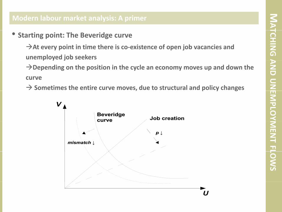
Modern labour market analysis: A primerTCH

INGA

• Starting point: The Beveridge curve

At every point in time there is co‐existence of open job vacancies and

unemployed job seekers ANDUNE

p y j

Depending on the position in the cycle an economy moves up and down the

curve

Sometimes the entire curve moves, due to structural and policy changes EMPLO

Y

, p y g

MEN

TFLLO

WS

MAT

Understanding labour market flows ITCH

INGA

Decomposing unemployment dynamics

ttttt OUTINELU −=Δ−Δ=Δ ANDUNE

ttttt

Labour force growth as a function of history and incentives

TLL βββ ΔΔΔ

EMPLO

Y

LttLtLtLLt TaxuLL εβββα ++Δ+Δ+=Δ −− 31211

MEN

TFL

• Labour force growth determined byHistorical trends (persistence)

Di d k ff (i β lik l b i )

LOWS

Discouraged worker effect (i.e. βL2 likely to be negative)

Tax incentives (and other non‐tax measures such as child

care provisions, etc.)

MAT

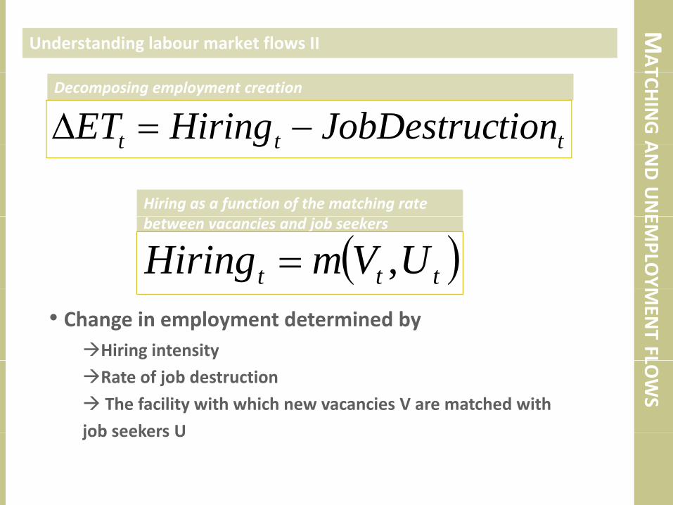
Understanding labour market flows IITCH

INGA

Decomposing employment creation

ttt tionJobDestrucHiringET −=Δ ANDUNE

ttt g

Hiring as a function of the matching rate EMPLO

Y

between vacancies and job seekers

( )ttt UVmHiring ,=

MEN

TFL

• Change in employment determined byHiring intensity LO

WS

Rate of job destruction

The facility with which new vacancies V are matched with

job seekers Ujob seekers U

MAT

Understanding labour market flows IIITCH

INGA

• Hiring depends on incentives to open vacancies (i.e. job creation) A

NDUNE

Demand factors: Investment, private consumption, external demand

Persistence effects: Past employment rates

Relative prices: Wages, user cost of capital EMPLO

Y

p g , p

Financial markets: Real share prices

Demand pressure on the labour market (labour market tightness)

MEN

TFLADwETnJobCreatio βββα +++

Job creation as a function of demand and supply factors

LOWS

JCttt

tttJCt

rVUADwETnJobCreatioεβββ

βββα++++

+++=

−

−

1654

3211

MAT

Understanding labour market flows IIITCH

INGA

•Job destruction is a function ofRelative prices: Wages, real interest rates, tax wedge

Schumpeter effect: TFP import competition

ANDUNE

Job destruction determined by technological and competitive forces

REERrTFPtionJobDestruc βββα +++=

Schumpeter effect: TFP, import competition

EMPLO

YJDttJDtJDtJD

tJDtJDtJDJDt

ADwIMPREERrTFPtionJobDestruc

εββββββα

+++++++=

654

321

MEN

TFL

•WagesNegotiation (Nash bargaining) between firms and workers

Distribution of producer rent (matching rent)

LOWS

Distribution of producer rent (matching rent)

Wages depend on reservation wages and bargaining power

( ) ( )ttttt UVUBw ,1 Π+−= γγ

MAT

Data and methodologyTCH

INGA

• Data:Macro data from OECD A

NDUNE

Unemployment flow estimates by Elsby et al. (2008)‐Estimated flows based on LFS information on unemployment

duration EMPLO

Y

duration

‐Match job creation/destruction rates under certain assumptions

• Methodology: MEN

TFL

Start with single‐equation identification

The estimate system of equations

Full macro‐model on the basis of GMM LOWS

Full macro‐model on the basis of GMM

MAT

Determinants of unemployment outflows IITCH

INGA

• Decomposition of unemployment outflows shows that:Demand components play an important role (>40%)

d f f l l ff ( )

ANDUNE

Indication for some financial accelerator effect (>30%)

Relative prices (wages) more moderate role (<20%)

EMPLO

YMEN

TFLLO

WS

MAT

Determinants of unemployment inflows IITCH

INGA

• Decomposition of unemployment inflows shows:No Schumpeterian effect from import penetration (strong

d d ff )

ANDUNE

demand effect)

Job churning due to changes in interest rates and TFP growth

EMPLO

YMEN

TFLLO

WS

MAT

A simple macro framework ITCH

INGA

• Unemployment flows influence each other:Higher job destruction rates increases unemployment pool...

h k h f f f ll

ANDUNE

This makes it cheaper for firms to fill vacancies...

This increases hiring and job creation rates...

...which makes it more difficult for other firms to find new EMPLO

Y

labour...

which lowers job creation rates, etc....

•An aggregate supply curve to understand interest rates: MEN

TFL

•An aggregate supply curve to understand interest rates:The basic labour flow model assumes fixed interest rates and

productivity LOWS

To analyse macroeconomic employment dynamics we need

an aggregate supply curve

MAT

A simple macro framework IITCH

INGA

• First step: Only fiscal policy reaction curveMutual dependence of unemployment flows on each other

l f h f h l b k

ANDUNE

A policy reaction function to the state of the labour market

Long‐term interest rate purely determined by changes in

government debt EMPLO

Y

No considerations to short‐term variations in private savings

(assuming historical trend)

Considering different fiscal and labour market policies MEN

TFLtitijttttt PolicyLMMacroOutflowsInflows ,,1 εα +++++= −

Considering different fiscal and labour market policies

individually

LOWS

tptpjttt

totojttttt

j

InflowsOutflowsPolicy

PolicyLMMacroInflowsOutflows ,,1

,,

εα

εα

+++=

+++++= −

trtrjtttt

tptpjttt

SavingsDebtPolicyRIRL

ffy

,,

,,

εα ++++=

MAT

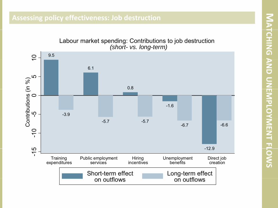
Assessing policy effectiveness: Job destructionTCH

INGA9.5

10Labour market spending: Contributions to job destruction

(short- vs. long-term)

ANDUNE

6.1

0.8

51

n %

)

EMPLO

Y-3.9

0.8

-1.6

-50

ntrib

utio

ns (i

MEN

TFL

-5.7 -5.7-6.7

12 9

-6.6

5-1

0C

on

LOWS

-12.9

-15

Trainingexpenditures

Public employmentservices

Hiringincentives

Unemploymentbenefits

Direct jobcreation

Short-term effecttfl

Long-term effecttflon outflows on outflows

MAT

Assessing policy effectiveness: Job creationTCH

INGA39.2

40Labour market spending: Contributions to job creation

(short- vs. long-term)

ANDUNE25.7

304

n %

)

EMPLO

Y15.7 15.6

20nt

ribut

ions

(in

MEN

TFL

5.3 4.0 3.5 3.5

7.5

2.8

10C

on

LOWS

0

Unemploymentbenefits

Hiringincentives

Trainingexpenditures

Public employmentservices

Direct jobcreation

Short-term effecton outflows

Long-term effecton outflowson outflows on outflows

MAT

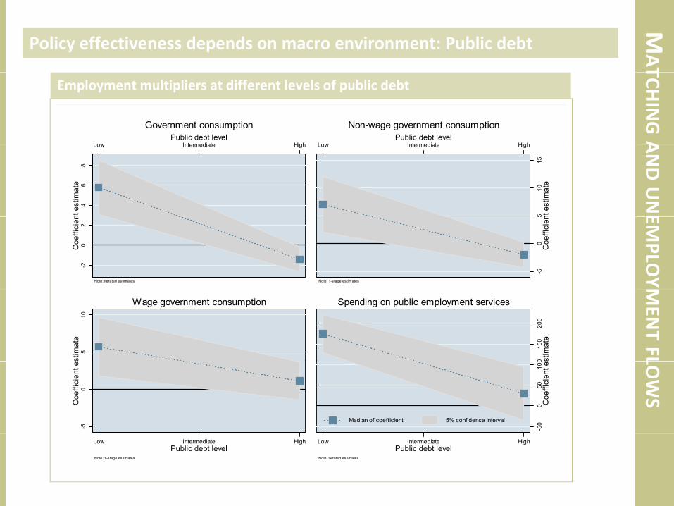
Policy effectiveness depends on macro environment: Public debtTCH

INGA

Low Intermediate HighPublic debt level

Government consumption


Non-wage government consumption

Employment multipliers at different levels of public debt

ANDUNE4

68

nt e

stim

ate

Low Intermediate High

510

15nt

est

imat

e

Low Intermediate High

EMPLO

Y-20

2C

oeffi

cien

Note: Iterated estimates

-50

5C

oeffi

cien

Note: 1-stage estimates MEN

TFL5

10st

imat

e

Wage government consumption

015

020

0st

imat

e

Spending on public employment services

LOWS

-50

Coe

ffici

ent e

s

-50

050

100

Coe

ffici

ent e

s

Median of coefficient 5% confidence interval


Note: 1-stage estimates



MAT

Policy effectiveness depends on environment: Structural unemployment

Hiring incentives

TCHINGA10

015

0st

imat

e

Hiring incentives

ANDUNE

050

Coe

ffici

ent e

sEM

PLOY

-50

Low Intermediate HighStructural unemployment rate


Training expenditures MEN

TFL

4060

estim

ate

g p

LOWS

200

20C

oeffi

cien

t e-2

Low Intermediate HighStructural unemployment rate


MAT

Policy effectiveness depends on environment: Financial crisis timesTCH

INGA15

Low Intermediate HighFinancial stress tercile

Government consumption

50

Low HighFinancial stress tercilePublic employment

ANDUNE0

510

effic

ient

est

imat

e

3040

effic

ient

est

imat

e

EMPLO

Y

-5C

oe


20C

oe


Direct job creation Unemployment benefits MEN

TFL30

040

0m

ate


010

0m

ate


LOWS

00

100

200

Coe

ffici

ent e

sti

050

Coe

ffici

ent e

sti

-100


-50


MAT

A simple macro framework IIITCH

INGA

• Second step: Endogenous short‐term interest ratesTaylor rule for interest rates

fl d

ANDUNE

New Keynesian inflation determination

Aggregate demand determined by state of the labour market

EMPLO

YMEN

TFLLO

WS

MAT

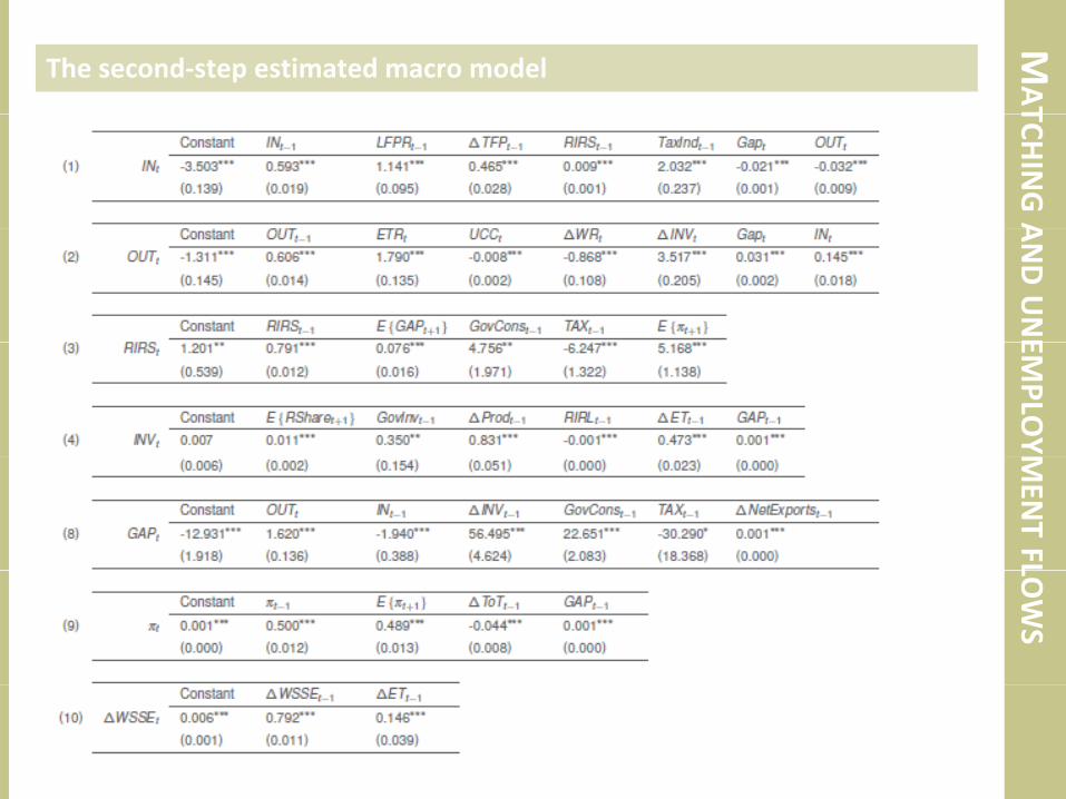
Using second‐step macro model for policy simulationTCH

INGA

• Estimation and simulationUsing GMM method to estimate the full model using panel

d

ANDUNE

data

Simulating the resulting model for the “average G20” country

Shock the model with the 2009 unemployment shock, i.e. the EMPLO

Y

baseline scenario should yield the average decline in

employment growth

Create three counter‐factuals: One austerity scenario and two MEN

TFL

Create three counter factuals: One austerity scenario and two

public deficit scenarios (spending vs. tax reduction)

Here: Only two alternative scenarios depicted LOWS

MAT

The second‐step estimated macro modelTCH

INGAANDUNEEM

PLOYM

ENTFLLO

WS

MAT

Employment recovery: The baseline scenarioTCH

INGAANDUNEEM

PLOYM

ENTFLLO

WS

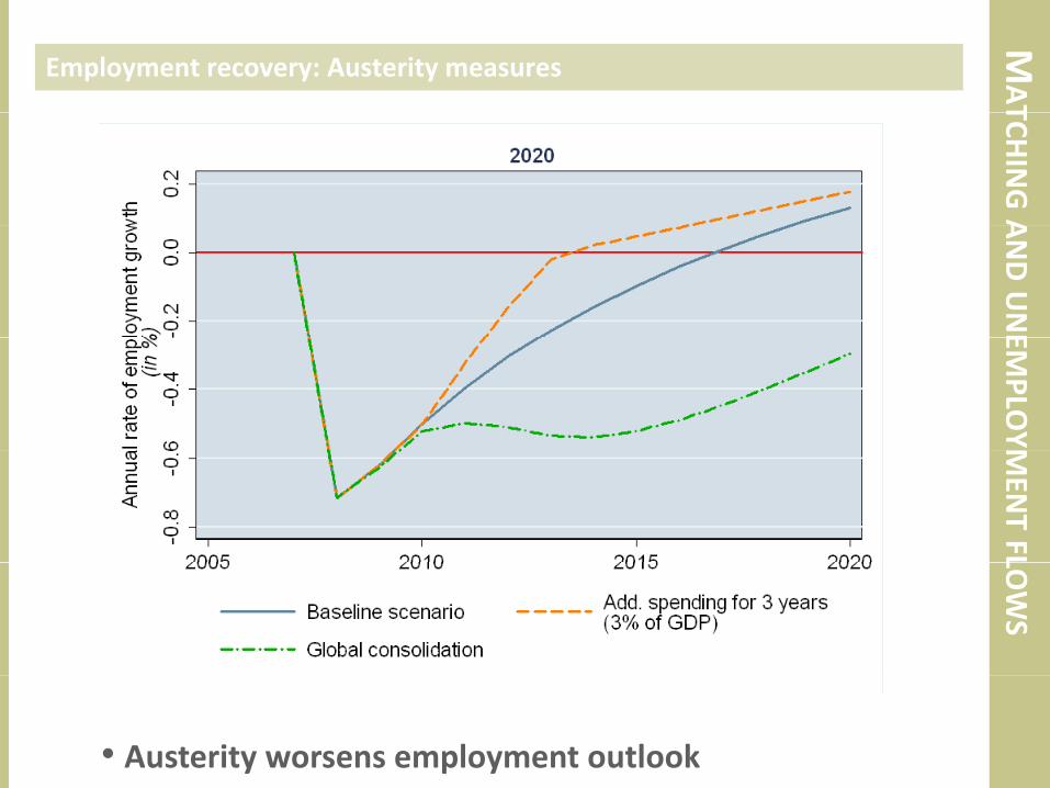
• Baseline scenarioBaseline scenarioRecovery in employment by 2017 to pre‐crisis trend growth

rates

MAT

Employment recovery: Additional stimulusTCH

INGAANDUNEEM

PLOYM

ENTFLLO

WS

• Additional stimulus pushes employment up

MAT

Employment recovery: Austerity measuresTCH

INGAANDUNEEM

PLOYM

ENTFLLO

WS

• Austerity worsens employment outlook

EXERRCISES

ExercisesExercises

EXER

Exercise 1: Labour market indicatorsRCISES

• Calculate labour market information from basic data for

TrinidadEmployment‐to‐population ratio

Unemployment rate

Sectoral employment ratesp y

Sectoral adjustment (annual frequency)

Average hours worked

EXER

Exercise 2: Employment elasticitiesRCISES

• Calculating employment elasticities for TrinidadCalculate annual GDP and employment growth rates

l l l l l ( h d)Calculate yearly employment elasticities (Arc‐method)

Calculate two 5‐year elasticities

Calculate the Point‐elasticity

Examine results

•On the basis of these employment elasticities…how big is the jobs gap between current and pre crisis…how big is the jobs gap between current and pre‐crisis

employment developments?

…how big would the jobs gap be next year with a GDP growth

rate that is only half as big as the current trend?

EXER

Exercise 3: Phillips curve for TrinidadRCISES

• Construct a structural unemployment rate for ToT:Use an historical average

l l f l dCalculate an HP filtered version

• Extract price inflation informationEstimate a basic Phillips curvep

How does the Phillips curve change with different estimates

for the structural unemployment rate

How much more unemplyoment is being generated byHow much more unemplyoment is being generated by

bringing the inflation rate down by 1 percentage point?

The EndThe End

if anything is unclear, please ask ! - international ... · Ædoes not cover people deciding to...

Documents