ifa fachpraktikum - experiment 2.2: self-erecting inverted pendulum
TRANSCRIPT

Automatic Control Laboratory, ETH ZurichProfs. M. Morari, J. Lygeros
Manual prepared by: Claudia Fischer, Aldo ZgraggenRevision from: September 22, 2014
IfA Fachpraktikum - Experiment 2.2:
Self-Erecting Inverted Pendulum
In this experiment, a pendulum is mounted on a cart. The pendulum shall be controlled to stayat its unstable equilibrium, i.e. the upright position. You will design a linear quadratic regulator(LQR) to achieve this goal.Additionally, you will implement a destabilizing controller that will make the pendulum swingup from its stable downward position. Finally, the two controllers will be combined to yield aself-erecting pendulum.
Figure 1: The inverted pendulum in the IfA lab.
For the preparation of this experiment at home you need to download the following files fromthe IfA Fachpraktikum website http://control.ee.ethz.ch/∼ifa-fp/ .
stabilizing control structure.m m-file structure for inverted pendulumswingup control structure.m m-file structure for self-erecting pendulum
During the lab session you will need additional files that are provided locally on your machine.

Contents
1 Problem Setup and Notation 3
2 Preparation@Home 52.1 Modeling . . . . . . . . . . . . . . . . . . . . . . . . . . . . . . . . . . . . . . . . 5Task 1: Nonlinear Differential Equations . . . . . . . . . . . . . . . . . . . . . . . . . . . . . . . . . . . . . . . . . . . . . . . 5Task 2: Linearization of the system . . . . . . . . . . . . . . . . . . . . . . . . . . . . . . . . . . . . . . . . . . . . . . . . . . . . 6Task 3: State space representation . . . . . . . . . . . . . . . . . . . . . . . . . . . . . . . . . . . . . . . . . . . . . . . . . . . . . 6Task 4: Numerical state space representation . . . . . . . . . . . . . . . . . . . . . . . . . . . . . . . . . . . . . . . . . . 62.2 Optimal State Feedback Control - LQR . . . . . . . . . . . . . . . . . . . . . . . 8Task 5: Theoretical considerations for LQR control . . . . . . . . . . . . . . . . . . . . . . . . . . . . . . . . . . . . 8Task 6: LQR controller gain . . . . . . . . . . . . . . . . . . . . . . . . . . . . . . . . . . . . . . . . . . . . . . . . . . . . . . . . . . . 82.3 Self-Erecting Pendulum Control . . . . . . . . . . . . . . . . . . . . . . . . . . . . 10Task 7: State space representation . . . . . . . . . . . . . . . . . . . . . . . . . . . . . . . . . . . . . . . . . . . . . . . . . . . . 10Task 8: Stabilizing position control parameters . . . . . . . . . . . . . . . . . . . . . . . . . . . . . . . . . . . . . . . 10Task 9: Destabilizing pendulum control parameters . . . . . . . . . . . . . . . . . . . . . . . . . . . . . . . . . . . 11Task 10: Switch to stabilizing control . . . . . . . . . . . . . . . . . . . . . . . . . . . . . . . . . . . . . . . . . . . . . . . . 11
3 Lab Session Tasks 123.1 Hardware Setup . . . . . . . . . . . . . . . . . . . . . . . . . . . . . . . . . . . . . 12
3.1.1 Safety precautions . . . . . . . . . . . . . . . . . . . . . . . . . . . . . . . 133.2 Inverted Pendulum Experiment . . . . . . . . . . . . . . . . . . . . . . . . . . . . 13
3.2.1 Simulation . . . . . . . . . . . . . . . . . . . . . . . . . . . . . . . . . . . 133.2.2 Controller Real-Time Implementation . . . . . . . . . . . . . . . . . . . . 13
3.3 Self-Erecting Pendulum . . . . . . . . . . . . . . . . . . . . . . . . . . . . . . . . 153.3.1 Simulation . . . . . . . . . . . . . . . . . . . . . . . . . . . . . . . . . . . 153.3.2 Controller Real-Time Implementation . . . . . . . . . . . . . . . . . . . . 15
4 Lessons Learnt 17Lesson Learnt 1: Model validity . . . . . . . . . . . . . . . . . . . . . . . . . . . . . . . . . . . . . . . . . . . . . . . . . . . . . 17Lesson Learnt 2: Tuning . . . . . . . . . . . . . . . . . . . . . . . . . . . . . . . . . . . . . . . . . . . . . . . . . . . . . . . . . . . . 17Lesson Learnt 3: Switching . . . . . . . . . . . . . . . . . . . . . . . . . . . . . . . . . . . . . . . . . . . . . . . . . . . . . . . . . 17Lesson Learnt 4: Completion of Experiment . . . . . . . . . . . . . . . . . . . . . . . . . . . . . . . . . . . . . . . . . 17
2

Chapter 1
Problem Setup and Notation
The inverted pendulum is a classic problem in dynamics and control theory. It is widely usedfor testing control algorithms. As opposed to the ordinary pendulum, the inverted pendulumhas its mass above its pivot point. Whereas the normal pendulum is stable when pointing down-wards, the inverted pendulum is inherently unstable. Therefore it must be actively balanced in
Figure 1.1: A pendulum is mounted on a cart. It can be stabilized in the upright position bymoving the cart accordingly.
order to remain upright. To that end, the inverted pendulum is mounted on a cart that canmove horizontally (Figure 1.1). As the stabilization of the pendulum is a nonlinear problem, thesystem must be linearized in order to be able to apply standard linear control methods.
3

Figure 1.2 shows a picture of the experimental setup you will find in the lab. The plant consists
Figure 1.2: Hardware setup of the inverted pendulum in the lab.
of three parts: the pendulum, the cart, and the track, which limits the movement of the cart.The orange box contains five fuses and plugs. All fuses must be set for the plugs to be live. Theblue box contains the black power module that provides the power for the motor of the cart,and the B&R industrial control unit comprising a CPU and counter modules, that processesthe measurements and computes the control inputs. All code and simulations are implementedusing the lab PC on the right.
4
Chapter 2
Preparation@Home
2.1 Modeling
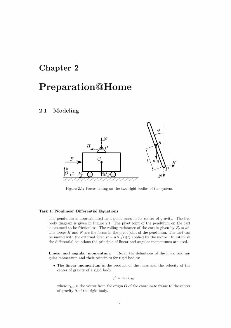
Figure 2.1: Forces acting on the two rigid bodies of the system.
Task 1: Nonlinear Differential Equations
The pendulum is approximated as a point mass in its center of gravity. The freebody diagram is given in Figure 2.1. The pivot joint of the pendulum on the cartis assumed to be frictionless. The rolling resistance of the cart is given by Fr = bx.The forces H and N are the forces in the pivot joint of the pendulum. The cart canbe moved with the external force F = nKt/ri(t) applied by the motor. To establishthe differential equations the principle of linear and angular momentums are used.
Linear and angular momentum: Recall the definitions of the linear and an-gular momentum and their principles for rigid bodies:
• The linear momentum is the product of the mass and the velocity of thecenter of gravity of a rigid body:
~p := m · ~rOS
where rOS is the vector from the origin O of the coordinate frame to the centerof gravity S of the rigid body.
5

• The angular momentum is the sum of the linear momentum of a stationarypoint of the rigid body and the spin of the body:
~Lp := m · ~rOS × ~rOS + ΘSφ
where rPS is the vector from the reference point P to the center of gravity S.
• The principle of linear momentum states that the derivative of the linearmomentum is equal to the sum of the forces acting on the system:
~p =∑
~Fi
• The principle of angular momentum states that the derivative of the an-gular momentum is equal to the sum of the induced moments acting on thebody:
~Lp =∑
~r0Bi× ~FBi
+∑
Mi
Proceed as follows:
1. Determine the linear momentum ~pc of the cart in x direction.
2. Take the first derivative of the linear momentum ~pc of the cart and set it equalto all forces acting on the cart in x direction.
3. Determine the linear momentum ~pp of the pendulum in x and y direction.
4. Take the first derivative of the linear momentum ~pp of the pendulum in bothdirections and set it equal to all forces acting on the pendulum in its respectivedirection.
5. Determine the angular momentum ~Lp of the pendulum.
6. Take the first derivative of the angular momentum ~Lp of the pendulum and setit equal to all moments acting on the pendulum.
7. Bring the system to the form x = f1(x, x, φ, φ, F ); φ = f2(x, x, φ, φ, F )
Task 2: Linearization of the system
In order to be able to apply linear control methods, this nonlinear system mustbe linearized. Use the method presented in the control systems lecture to linearizethe system around its unstable equilibrium φ = 0, x = 0, φ = 0, F = 0, i.e.xss = [0, 0, 0, 0], uss = 0.
Task 3: State space representation
Write the linearized system in state space representation.
6

Task 4: Numerical state space representation
Include the state space representation in the Matlab script stabilizing control structure.m.Save it as stabilizing control.m. The numerical parameters are:
pendulum mass m 0.104kgcart mass M 1.79kgpendulum length from pivot to center of gravity l 0.1524mgravitational acceleration g 9.81ms2friction coefficient b 0.001Nsmmotor efficiency n 1motor torque constant Kt 0.07NmAmotor pinion radius r 6.35e− 3mforce acting on the cart F n·Kt
r · i(t)
7

2.2 Optimal State Feedback Control - LQR
To keep the pendulum in the upright position, a stabilizing state feedback controller shall beimplemented. The corresponding block diagram is given in Figure 2.2.(xref , φref , xref , φref ) is the state reference. The reference angle φref must be equal to the
unstable equilibrium π. The pendulum’s and cart’s velocities φref and xref must be zero.The cart position does not influence the equilibrium, its reference xref can therefore be chosenarbitrarily inside its allowed range.The task here is to find an optimal feedback controller, i.e. a linear quadratic regulator (LQR)that stabilizes the system.
Figure 2.2: Block diagram of the state feedback system.
The idea behind LQR is to find a feedback gain KLQR, such that the control law
u(t) = −KLQRx
minimises the cost function
J(u(t)) =
∫ ∞0
x(t)TQx(t) + u(t)TRu(t)dt
and stabilises the closed control loop (||x(t)|| → 0, and ||u(t)|| → 0 as t→∞) while keeping thecontrol energy as small as possible or within certain bounds.
The optimal feedback gain KLQR can be obtained using the Matlab command lqr. Forfurther mathematical details of LQR, please refer to the control systems lecture notes.
Task 5: Theoretical considerations for LQR control
1. What are the dimensions of the Q-matrix?
2. Which matrix properties are necessary for Q? Why?
3. What are the dimensions of the R-matrix?
4. Which matrix properties are necessary for R? Why?
5. How is the control behaviour affected if you choose much larger values for theentries of Q than for R? What problems may occur?
6. What happens in the opposite case?
7. What happens if you increase/decrease the entries of Q and R at the same rate?
8. What is the impact of a deviation of the position of the cart from the equilibriumstate, what is the impact of a deviation in the pendulum angle? What does thismean for the tuning of Q?
9. What are the units of the states and what is the expected maximum deviation?What does this mean for the tuning of Q?
Hint: Helpful information can be found in the RS1 lecture notes chapter 13
8

Task 6: LQR controller gain
The next step is to define the matrices Q and R and compute the gain K. Forthe sake of comparison to the master solution, keep R = 1 and only tune Q. Thecontroller should be rather fast, but not too aggressive in order not to violate thecurrent saturation constraints. You can compute K in stabilizing control.m usingthe Matlab command ’lqr’ !
9

2.3 Self-Erecting Pendulum Control
The final goal of this experiment is to obtain a self-erecting pendulum. To that end, a destabi-lizing controller for the angle (swing-up controller) must be implemented.
Figure 2.3: Schematics of the cascaded control of the swing-up motion.
The control of the position of the cart needs to be stable to keep the cart on the track.The idea is to have a cascaded control with an inner loop that stabilizes the cart’s position,and an outer control loop that destabilizes the pendulum’s down-equilibrium by calculating acorresponding cart position reference (Figure 2.3).To obtain a self-erecting pendulum, switching between the swing-up and the stabilizing controlleris necessary. This is denoted “mode selection” in Figure 2.4. Once the pendulum position reachesan angle from which it can be stabilized, the control is switched from swing-up to stabilizing.
Figure 2.4: Schematics of the self-erecting pendulum control.
For the following tasks, use the file swingup control structure.m. Save the edited code asswingup control.m.
Task 7: State space representation
For the stabilizing position control, calculate the model of the reduced system(x, x). Neglect the dependence on φ.
10
Task 8: Stabilizing position control parameters
The poles shall be placed at −7 and −15, respectively. Determine the correspondinggain Kpos using Ackerman’s pole placement formula! Hint: Use the Matlab com-mand ’place’.
Task 9: Destabilizing pendulum control parameters
For the position reference, consider x = P · φ + D · φ, where [P,D] = Kφ, andP ∈ R, D ∈ R. How should the cart respond to the pendulum angle in order toswing up?Remark: φ = 0 is the stable equilibrium (pendulum pointing downwards), φ = π isthe upright position.
Task 10: Switch to stabilizing control
To stabilize the pendulum in the upright position, one must switch to the stabiliz-ing controller once the pendulum has reached an angle close enough to the uprightposition (φ = π). What angle would you choose?
11
Chapter 3
Lab Session Tasks
The lab session consists of two parts: In a first step, the homework results will be testedin a Simulink model. In a second step, the feedback control will be employed in the actualexperimental setup.
3.1 Hardware Setup
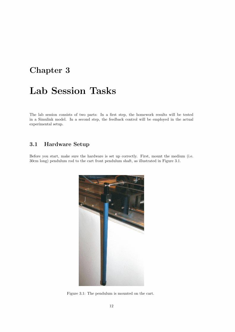
Before you start, make sure the hardware is set up correctly. First, mount the medium (i.e.30cm long) pendulum rod to the cart front pendulum shaft, as illustrated in Figure 3.1.
Figure 3.1: The pendulum is mounted on the cart.
12

3.1.1 Safety precautions
• For safety reasons ensure that there is about 1m of clearance from either end of the trackat any time to avoid collisions.
• Before you start experiments, put the cart to the middle of the track.
• Verify that the suspended pendulum is not moving before starting the system.
• If you change any parameters, e.g. K, always verify the new controller with the Simulinkmodel first. Before implementing the controller on the actual system, you must ensure thespecifications are met without saturating the actuator.
• Ensure you are always able to safely reach the emergency stop button.
3.2 Inverted Pendulum Experiment
To start the session in the lab, right-click the icon ifa 2.2 on the desktop of the lab computerand select ’run with power shell’. This will download all necessary files and start Matlab. Torun Matlab scripts, just type their name in the Matlab command window.
3.2.1 Simulation
The next step is to test the controller designed in the homework in a model. First, run ifa2 2aif not done automatically. This will:
• change the Matlab directory to the correct folder, and
• open the necessary Simulink model InvertedPendulum.mdl.
Copy the Matlab script file stabilizing control.m prepared in the homework to the currentMatlab folder and run it. Run the Simulink model.Investigate the model behaviour for different tuning parameters in Q! Check if the constraints onthe cart postion (±500mm) and the controller input (±15A) are respected! Save the improvedversion of stabilizing control.m to the current folder.
3.2.2 Controller Real-Time Implementation
The next step is to implement the previously designed controller on the hardware. Run ifa2 2b.This will:
• change the Matlab directory to the correct folder, and
• open the Simulink model InvertedPendulum Real.mdl.
Copy the Matlab script file stabilizing control.m with the improved parameters found in thesimulation (section 3.2.1) to the current Matlab folder.
Preparation and implementation
• Before you start, make sure that save operation is guaranteed and the parameters areset accordingly (check with simulation!).
• Run ’START InvertedPendulum.m’ to initialize the amplifiers and setup the hard-ware.
• Ensure the real-time code is run safely by manually moving the cart to the middleof the track so it is free to move to both sides. The LED on the black power moduleshould turn green.
• In order to observe the system’s real-time responses, use the scope in the Simulink model.
13

Figure 3.2: Press first a) to build the model, and then b) to connect to the target.
Execution
1. As depicted in Fig. 3.2 press a) to build the Simulink model.
2. You will be asked twice to enter the path to B&R Automation Studio in the Matlabcommand line. The path is C:\Program Files\BrAutomation\AS30090
3. In the Simulink model, press b) to connect to the target.
4. To activate the controller, set the ’manual allow signal’ in the Simulink file to 1. Then,slowly rotate the pendulum counterclockwise to the upright position (the cart will beginto move). Release the pendulum as soon as the controller is activated.
5. The cart should now track the position reference and regulate the pendulum angle to 180o.
6. Also, try introducing a disturbance by gently poking the tip of the rod.
7. Set the ’manual allow signal’ in the Simulink file back to 0 and disconnect from the target(button b)) if you want to stop the real-time execution or change the gain K. You do notneed to rebuild the project after changing K, it is sufficient to restart from 3.
14

3.3 Self-Erecting Pendulum
In a second experiment, we want to implement a self-erecting pendulum. As before, in a firststep simulations must be run to check the homework results. Run ifa2 2c. This will
• change the Matlab directory to the correct folder, and
• open the necessary Simulink model SelfErectingPendulum.mdl.
Copy the Matlab script file swingup control.m from your homework to the current folder andrun it.
3.3.1 Simulation
The simulink model consists of two parts: the swing-up control and the stabilizing invertedpendulum control. Corresponding to the pendulum angle, the respective controller is active.The model also includes a small angular excitation.
• Set the switching angle to 3rad.
• Run swingup control.m and stabilizing control.m. Run SelfErectingPendulum.mdl. Arethe simulation results satisfactory?
• Tune Kpos, P and D and compare the results!
• Run SelfErectingPendulum.mdl with different switching angles, e.g. 2rad, 2.5rad, 3rad.Which ones yield satisfactory results?
• Is this control save in terms of physical limitations (e.g. cart position)?
• Save the improved version of swingup control.m to the current Matlab directory.
3.3.2 Controller Real-Time Implementation
For the self-erecting pendulum control, run ifa2 2d. This will
• change the Matlab directory to the correct folder, and
• open the Simulink model SelfErectingPendulum Real.mdl.
Copy your improved version of swingup control.m to the current Matlab directory.
Preparation and implementation
• Before you start, make sure that save operation is guaranteed and the parameters areset accordingly (see simulation!).
• Run START SelfErectingPendulum.m to initialize the amplifiers and setup the hard-ware.
• Ensure the real-time code is run safely by manually moving the cart to the middleof the track so it is free to move to both sides. The LED on the black power moduleshould turn green.
• In order to observe the system’s real-time responses, use the scope in the Simulink model.
15

Execution
• To start the experiment, proceed as in the first point described in section 3.2.2 and Fig.3.2.
• To activate the controller, poke the pendulum VERY gently. The pendulum will startto swing up.
• Set the ’manual allow signal’ in the Simulink file back to 0 and then press button b) (Fig.3.2) again if you want to stop the real-time execution.
16

Chapter 4
Lessons Learnt
An inverted pendulum can be stabilized using a state feedback controller based on a linearizedmodel of the pendulum. The cart on which the pendulum is mounted is able to follow a giventrajectory while keeping the pendulum in the upright position. Furthermore, it is possibleto implement a self-erecting pendulum using feedback that destabilizes the stable pendulumposition.
Lesson Learnt 1: Model validity
In the simulation, for which range of starting angles does the stabilizing controllerwork? Why?
Lesson Learnt 2: Tuning
What happens if you tune the destabilizing parameters for the self-erecting pendulumtoo aggressively?
Lesson Learnt 3: Switching
What happens if you switch at an inadequate angle?
Lesson Learnt 4: Completion of Experiment
Please, fill out the online feedback form on the registration page under MyExperiments.Each student/participant has to fill out its own feedback form. This will help us toimprove the experiment. Thank you for your help.
17