ih3214741491

S.Poorna Chander Rao / International Journal of Engineering Research and Applications

(IJERA) ISSN: 2248-9622 www.ijera.com

Vol. 3, Issue 2, March -April 2013, pp.1474-1491

1474 | P a g e

Enhancement Of Fast Loop Controlling Mechanism For

Capacitor- Supported Dynamic Voltage Restorer (DVR) Using

Modulation Technique

S.Poorna Chander Rao Department of Electrical Engineering, JNTU Hyderabad, Hyderabad-500085

ABSTRACT :-The power quality (PQ)

requirement is one of the most important issues for

power companies and their customers. The power

quality disturbances are voltage sag, swell, notch,

spike and transients etc. The dynamic voltage

restorer (DVR) is one of the modern devices used

in distribution systems to protect consumers

against sudden changes in voltage magnitude. The

analysis for a fast transient control scheme for

three phase capacitor-supported dynamic voltage

restorer (DVR) is presented in this paper. This

work provides us to find the optimal location and

the optimal DVR settings to enhance the

distribution related loading issues. Conventional

voltage-restoration technique is based on injecting

voltage being in-phase with the supply voltage. The

injected voltage magnitude will be the minimum,

but the energy injected by the DVR is no minimal.

In order to minimize the required capacity of the

dc source, a minimum energy injection concept is

taken into the considerations. It is based on

maximizing the active power delivered by the

supply mains and the reactive power handled by

the DVR during the sag and swell cases. The

review model has been built and tested the

dynamic behaviors of the model under different

sagged and swelled conditions and depths will be

investigated. The quality of the load voltage under

unbalanced and distorted phase voltages, and

nonlinear inductive load is analyzed.

Keywords – Voltage sag, voltage swell, dynamic voltage restoration(DVR), power quality, total

harmonic reduction

I. INTRODUCTION Electronic systems operate properly as long

as the supply voltage stays within a consistent range.

There are several types of voltage fluctuations that can cause the systems to malfunction, including

surges and spikes, sags, harmonic distortions, and

momentary disruptions. Among them, voltage sag is

the major power-quality problem. It is an

unavoidable brief reduction in the voltage from

momentary disturbances, such as lightning strikes

and wild animals, on the power system. Although

most of them last for less than half a second, this is

often long enough for many types of loads to drop

out. Typical examples include variable speed drives,

motor starter

contactors, control relays, and programmable logic controllers. Such an unplanned stoppage can cause

the

load to take a long time to restart and can lead to high

cost of lost production.

Dynamic voltage restorer (DVR) is

presently one of the most cost-effective and thorough

solutions to mitigate voltage sags by establishing

proper quality voltage level for utility customers [3].

Its function is to inject a voltage in series with the

supply and compensate for the difference between the

nominal and sagged supply voltage. The injected voltage is typically provided by an inverter, which is

powered by a dc source, such as batteries, flywheels,

externally powered rectifiers, and capacitors.

Voltage restoration involves determining the

amount of energy and the magnitude of the voltage

injected by the DVR. Conventional voltage-

restoration technique is based on injecting a voltage

being in-phase with the supply voltage. The injected

voltage magnitude will be the minimum, but the

energy injected by the DVR is non minimal.

In order to minimize the required capacity of

the dc source, a minimum energy injection (MEI) concept is proposed in. It is based on maximizing the

active power delivered by the supply mains and the

reactive power handled by the DVR during the sag.

Determination of the injected-voltage magnitude is

based on a real-time iterative method to minimize the

active power injection by the DVR. This can then

enhance the ride-through capability. However, the

operation of each phase is individually controlled.

There is no energy interaction between the un sagged

phase(s) and the sagged phase(s), in order to enhance

the voltage restoration. Moreover, as the computation method is purely based on sinusoidal waveforms, the

implementation is complicated in distribution

network with nonlinear load. A sliding window over

one line cycle of the fundamental frequency is

proposed to determine the active and reactive power

at the fundamental frequency. The lengthy

computation time of the injected voltage phasor will

cause output distortion after voltage sag.

Instead of using an external energy storage

device, the methods are taking the active power for

the inverter from the transmission system via a shunt-

connected rectifier. The series inverter by its self has the capability to provide real-series compensation to

the line. The rectifier-based source requires a separate

service supply, while the battery-based source




1475 | P a g e

requires regular maintenance and is not environment

friendly. No external source is required in the DVR.

The required phase and magnitude of the inverter

load-voltage phasor are derived by considering the energy balance between the supply and the load, but

the advantage is offset by the lengthy digital

transformation and inversion of symmetrical

components and calculation of the power

consumption. The wave shape of the load voltage

will be distorted and will take a relatively long

settling time. As the supply voltage is assumed to be

sinusoidal in the calculation, the load voltage will be

affected and distorted with non sinusoidal supply

voltage and load current. A single-phase capacitor-

supported DVR can ideally revert the

Fig.1. Proposed DVR structure

load voltage to steady state in two switching actions after voltage sags. By extending the concept, an

analog-based three-phase capacitor-supported

interline DVR is presented [19]–[21].

II. HEADINGS 1. INTRODUCTION

2. DYNAMIC VOLTAGE RESTORER

2.1. Introduction

2.1.1. Voltage Source Converter 2.1.2. Boost or Injection Transformers

2.1.3. Passive Filters

2.1.4. Energy Storage

2.2. Control Strategy

2.2.1. Pre-Sag Compensation

2.2.2. In-Phase Compensation

2.2.3. Minimum Energy Compensation

2.3. Control and Protection

2.4. Summary

3. INVERETER

3.1. Introduction

3.1.1. Basic Designs 3.1.2. Total Harmonic Distortion

3.2. Single-Phase Voltage Source Inverter

3.2.1. Types of VSI

3.3. Applications

3.4. Summary

4. MODELING OF DVR

4.1. Principles of Operation

4.2. Review of Inner Loop

4.3. Characteristics of Outer Loop

4.4. Simplified Design Procedures

4.5 Results Analysis 4.5.1. Harmonic Distortions

4.5.2. Voltage Sag

4.5.3. Voltage Swell

4.6. Comparision of results with and without DVR

5. CONCLUSION

6. REFERENCES

III. DYNAMIC VOLTAGE RESTORER: 2.1. INTRODUCTION

The major objectives are to increase the

capacity utilization of distribution feeders (by

minimizing the rms values of the line currents for a

specified power demand), reduce the losses and

improve power quality at the load bus. The major

assumption was to neglect the variations in the source

voltages. This essentially implies that the dynamics

of the source voltage is much slower than the load

dynamics. When the fast variations in the source

voltage cannot be ignored, these can affect the

performance of critical loads such as (a) semiconductor fabrication plants (b) paper mills (c)

food processing plants and (d) automotive assembly

plants. The most common disturbances in the source

voltages are the voltage sags or swells that can be due

to

i) Disturbances arising in the

transmission system

ii) Adjacent feeder faults and

iii) Fuse or breaker operation.

Voltage sags of even 10% lasting for 5-10 cycles

can result in costly damage in critical loads. The voltage sags can arise due to symmetrical or

unsymmetrical faults. In the latter case, negative and

zero sequence components are also present.

Uncompensated nonlinear loads in the distribution

system can cause harmonic components in the supply

voltages. To mitigate the problems caused by poor

quality of power supply, series connected

compensators are used. These are called as Dynamic

Voltage Restorer (DVR) in the literature as their

primary application is to compensate for voltage sags

and swells. Their configuration is similar to that of

SSSC. However, the control techniques are different.




1476 | P a g e

Also, a DVR is expected to respond fast (less than

1/4 cycle) and thus employs PWM converters using

IGBT or IGCT devices. The first DVR entered

commercial service on the Duke Power System in U.S.A. in August 1996. It has a rating of 2 MVA with

660 kJ of energy storage and is capable of

compensating 50% voltage sag for a period of 0.5

second (30 cycles). It was installed to protect a highly

automated yarn manufacturing and rug weaving

facility. Since then, several DVRs have been installed

to protect microprocessor fabrication plants, paper

mills etc. Typically, DVRs are made of modular

design with a module rating of 2 MVA or 5 MVA.

They have been installed in substations of voltage

rating from 11 kV to 69 kV. A DVR has to supply energy to the load during the voltage sags. If a DVR

has to supply active power over longer periods, it is

convenient to provide a shunt converter that is

connected to the DVR on the DC side. As a matter of

fact one could envisage a combination of

DSTATCOM and DVR connected on the DC side to

compensate for both load and supply voltage

variations. In this section, we discuss the application

of DVR for fundamental frequency voltage. The

voltage source converter is typically one or more

converters connected in series to provide the required

voltage rating. The DVR can inject a (fundamental frequency) voltage in each phase of required

magnitude and phase. The DVR has two operating

modes

A. Standby (also termed as short circuit

operation (SCO) mode) where the voltage

injected has zero magnitude.

B. Boost (when the DVR injects a required

voltage of appropriate magnitude and phase

to restore the prefault load bus voltage).

The power circuit of DVR shown in Fig. 2.1 has four

components listed below 2.1.1. Voltage Source Converter (VSC):

This could be a 3 phase - 3 wire VSC or 3

phase - 4 wire VSC. The latter permits the injection

of zero-sequence voltages. Either a conventional two

level converter (Graetz bridge) or a three level

converter is used.

2.1.2. Boost or Injection Transformers:

Three single phase transformers are

connected in series with the distribution feeder to

couple the VSC (at the lower voltage level) to the

higher distribution voltage level. The three single transformers can be connected with star/open star

winding or delta/open star winding. The latter does

not permit the injection of the zero sequence voltage.

The choice of the injection transformer winding

depends on the connections of the step down

transformer that feeds the load. If ac Y connected

transformer (as shown in Fig. 2.1) is used, there is no

need to compensate the zero sequence voltages.

However if Y|Y connection with neutral grounding is

used, the zero sequence voltage may have to be

compensated. It is essential to avoid the saturation in

the injection transformers.

Fig. 2.1 Power circuit of DVR

2.1.3. Passive Filters:

The passive filters can be placed either on

the high voltage side or the converter side of the

boost transformers. The advantages of the converter

side filters are (a) the components are rated at lower voltage and (b) higher order harmonic currents (due

to the VSC) do not °own through the transformer

windings. The disadvantages are that the filter

inductor causes voltage drop and phase (angle) shift

in the (fundamental component of) voltage injected.

This can affect the control scheme of DVR. The

location of the filter o the high voltage side

overcomes the drawbacks (the leakage reactance of

the transformer can be used as a filter inductor), but

results in higher ratings of the transformers as high

frequency currents can °ow through the windings. 2.1.4. Energy Storage:

This is required to provide active power to

the load during deep voltage sags. Lead-acid

batteries, flywheel or SMES can be used for energy

storage. It is also possible to provide the required

power on the DC side of the VSC by an auxiliary

bridge converter that is fed from an auxiliary AC

supply.

2.2. CONTROL STRATEGY

There are three basic control strategies as follows:

2.2.1. Pre-Sag Compensation:

The supply voltage is continuously tracked and the load voltage is compensated to the pre-sag

condition. This method results in (nearly) undisturbed

load voltage, but requires higher rating of the DVR.

Before a sag occur, VS = VL = VO. The voltage sag

results in drop in the magnitude of the supply voltage

to VS1. The phase angle of the supply also may shift

see Fig. 2.2. The DVR injects a voltage VC1 such

that the load voltage (VL = VS1 + VC1) remains at VO

(both in magnitude and phase). It is claimed that

some loads are sensitive to phase jumps and it is

necessary to compensate for both the phase jumps and the voltage sags.




1477 | P a g e

Fig 2.2 Pre-Sag Compensation Phasor diagram

2.2.2. In-phase Compensation:

The voltage injected by the DVR is always

in phase with the supply voltage regardless of the

load current and the pre-sag voltage (VO). This

control strategy results in the minimum value of the

injected voltage (magnitude). However, the phase of

the load voltage is disturbed. For loads which are not

sensitive to the phase jumps, this control strategy

results in optimum utilization of the voltage rating of

the DVR. The power requirements for the DVR are

not zero for these strategies.

2.2.3. Minimum Energy Compensation: Neglecting losses, the power requirements

of the DVR are zero if the injected voltage (VC) is in

quadrature with the load current. To raise the voltage

at the load bus, the voltage injected by the DVR is

capacitive and VL leads VS1 (see Fig. 2.3). Fig. 2.3

also shows the in-phase compensation for

comparison. It is to be noted that the current phasor is

determined by the load bus voltage phasor and the

power factor of the load.

Fig 2.3 Minimum Energy Compensation Phasor

diagram

Implementation of the minimum energy

compensation requires the measurement of the load

current phasor in addition to the supply voltage.

When VC is in quadrature with the load current, DVR

supplies only reactive power. However, full load

voltage compensation is not possible Unless the

supply voltage is above a minimum value that

depends on the load power factor. When the

magnitude of VC is not constrained, the minimum value of VS that still allows full compensation is

where Á is the power factor angle and VO is the

required magnitude of the Load bus voltage. If the

magnitude of the injected voltage is limited (V max C ),

the minimum supply voltage that allows full

compensation is given by the expressions figures

(2.1) and (2.2). Note that at the minimum source

voltage, the current is in phase with VS for the case

(a).

2.3. CONTROL AND PROTECTION:

The control and protection of a DVR

designed to compensate voltage sags must consider

the following functional requirements. 1. When the supply voltage is normal, the

DVR operates in a standby mode with zero voltage

injection. However if the energy storage device (say

batteries) is to be charged, then the DVR can operate

in a self- charging control mode.

2. When a voltage sag/swell occurs, the

DVR needs to inject three single phase voltages in

synchronism with the supply in a very short time.

Each phase of the injected voltage can be controlled

independently in magnitude and phase. However,

zero sequence voltage can be eliminated in situations where it has no effect. The DVR draws active power

from the energy source and supplies this along with

the reactive power (required) to the load.

3. If there is a fault on the downstream of

the DVR, the converter is by- passed temporarily

using thyristor switches to protect the DVR against

over currents. The threshold is determined by the

current ratings of the DVR.

The overall design of DVR must consider

the following parameters:

1. Ratings of the load and power factor

2. Voltage rating of the distribution line 3. Maximum single phase sag (in percentage)

4. Maximum three phase sag (in percentage)

5. Duration of the voltage sag (in milliseconds)

6. The voltage time area (this is an indication of the

energy requirements)

7. Recovery time for the DC link voltage to 100%

Typically, a DVR may be designed to

protect a sensitive load against 35% of three phase

voltage sags or 50% of the single phase sag. The

duration of the sag could be 200 ms. The DVR can

compensate higher voltage sags lasting for shorter durations or allow longer durations up to 500 ms for

smaller voltage sags. The response time could be as

small as 1 ms.

2.4. SUMMARY:

DVR is used in the power system network

mainly to mitigate the power quality issues related to

voltage sags and voltage swells. It contains fast

dynamic switching devices like IGBT to facilitate

fast switching action and has a frequency of 10 KHz.

The voltage source inverters converts AC to DC

supply to charge the capacitor banks when a swell occurs and converts DC to AC supply and injects a

voltage in series with the line to overcome the effect

of voltage sag. The components used in the DVR

model are VSC, boosting transformer, passive filters

to overcome the harmonics which while switching

the IGBTs. To reduce the cost required by the storage

devices we can opt for a closed loop control to charge

the capacitor banks from the supply itself irrespective

of sagged or swelled conditions.




1478 | P a g e

3. INVERETER

3.1. INTROCTION:

The main objective of static power

converters is to produce an ac output waveform from a dc power supply. These are the types of waveforms

required in adjustable speed drives (ASDs),

uninterruptible power supplies (UPS), static var

compensators, active filters, flexible ac transmission

systems (FACTS), and voltage compensators, which

are only a few applications. For sinusoidal ac outputs,

the magnitude, frequency, and phase should be

controllable. According to the type of ac output

waveform, these topologies can be considered as

voltage source inverters (VSIs), where the

independently controlled ac output is a voltage waveform.

These structures are the most widely used

because they naturally behave as voltage sources as

required by many industrial applications, such as

adjustable speed drives (ASDs), which are the most

popular application of inverters; see Fig 3.1.

Similarly, these topologies can be found as current

source inverters (CSIs), where the independently

controlled ac output is a current waveform. These

structures are still widely used in medium-voltage

industrial applications, where high-quality voltage

waveforms are required. Static power converters, specifically inverters, are constructed from power

switches and the ac output waveforms are therefore

made up of discrete values. This leads to the

generation of waveforms that feature fast transitions

rather than smooth ones. For instance, the ac output

voltage produced by the VSI of a standard ASD is a

three-level

Fig 3.1 Inverter DC link

3.1.1. Basic designs:

In one simple inverter circuit, DC power is

connected to a transformer through the centre tap of

the primary winding. A switch is rapidly switched

back and forth to allow current to flow back to the

DC source following two alternate paths through one

end of the primary winding and then the other. The

alternation of the direction of current in the primary winding of the transformer produces alternating

current (AC) in the secondary circuit.The

electromechanical version of the switching device

includes two stationary contacts and a spring

supported moving contact. The spring holds the

movable contact against one of the stationary

contacts and an electromagnet pulls the movable

contact to the opposite stationary contact. The current in the electromagnet is interrupted by the action of

the switch so that the switch continually switches

rapidly back and forth. This type of

electromechanical inverter switch, called a vibrator or

buzzer, was once used in vacuum tube automobile

radios. A similar mechanism has been used in door

bells, buzzers and tattoo. As they became available

with adequate power ratings, transistors and various

other types of semiconductor switches have been

incorporated into inverter circuit designs.

Fig 3.2 switching of MOSFET

The switch in the simple inverter described

above, when not coupled to an output transformer,

produces a square voltage waveform due to its simple

off and on nature as opposed to

the sinusoidal waveform that is the usual waveform

of an AC power supply. Using Fourier

analysis, periodic waveforms are represented as the sum of an infinite series of sine waves. The sine wave

that has the same frequency as the original waveform

is called the fundamental component. The other sine

waves, called harmonics, which are included in the

series have frequencies that are integral multiples of

the fundamental frequency. The quality of the

inverter output waveform can be expressed by using

the Fourier analysis data to calculate the total

harmonic distortion (THD) Fig3.3. The total

harmonic distortion is the square root of the sum of

the squares of the harmonic voltages divided by the

fundamental voltage:

THD = …3.1

http://en.wikipedia.org/wiki/Transformer

http://en.wikipedia.org/wiki/Alternating_current



http://en.wikipedia.org/wiki/Vibrator_(electronic)

http://en.wikipedia.org/wiki/Vacuum_tube

http://en.wikipedia.org/wiki/Transistors

http://en.wikipedia.org/wiki/Semiconductor

http://en.wikipedia.org/wiki/Waveform

http://en.wikipedia.org/wiki/Sine_wave

http://en.wikipedia.org/wiki/Fourier_analysis



http://en.wikipedia.org/wiki/Periodic_function

http://en.wikipedia.org/wiki/Frequency

http://en.wikipedia.org/wiki/Total_harmonic_distortion






1479 | P a g e

Fig 3.3 Total harmonic distortion

3.2. Single-Phase Voltage Source Inverter:

Single-phase voltage source inverters

(VSI’s) can be found as half-bridge and full-bridge

topologies. Although the power range they cover is the low one, they are widely used in power supplies,

single-phase UPS’s, and currently to form elaborate

high-power static power topologies, such as for

instance, the multi cell configurations that are

reviewed. The main features of both approaches are

reviewed and presented in the following.

3.2.1. Types of VSI:

A. Half-Bridge VSI:

The power topology of a half-bridge VSI,

where two large capacitors are required to provide a neutral point N, such that each capacitor maintains a

constant voltage=2. Because the current harmonics

injected by the operation of the inverter are low-order

harmonics, a set of large capacitors (C. and Cÿ) is

required. It is clear that both switches S. and Sÿ

cannot be on simultaneously because short circuit

across the dc link voltage source Vi would be

produced. In order to avoid the short circuit across

the DC bus and the undefined ac output voltage

condition, the modulating technique should always

ensure that at any instant either the top or the bottom

switch of the inverter leg is on.

Fig 3.4 Half-bridge inverter

shows the ideal waveforms associated with the half-

bridge inverter shown in Fig 3.4. The states for the

switches S. and Sÿ are defined by the modulating

technique, which in this case is a carrier-based PWM. The Carrier-Based Pulse width Modulation (PWM)

Technique: As mentioned earlier, it is desired that the

ac output voltage. Va,N follow a given waveform

(e.g., sinusoidal) on a continuous basis by properly

switching the power valves. The carrier-based PWM

technique fulfils such a requirement as it defines the

on and off states of the switches of one leg of a VSI

by comparing a modulating signal Vc (desired ac

output voltage) and a triangular waveform Vd (carrier signal). In practice, when Vc > Vd the switch S. is on

and the switch is off; similarly, when Vc < Vd the

switch S. is off and the switch Sÿ is on. A special

case is when the modulating signal Vc is a sinusoidal

at frequency fc and amplitudeVc, and the triangular

signal Vd is at frequency fD and amplitude Vd. This is

the sinusoidal PWM (SPWM) scheme. In this case,

the modulation index ma (also known as the

amplitude-modulation ratio) is defined as

= …3.2

And the normalized carrier frequency mf (also known

as the frequency-modulation ratio) is

= …3.3

. VaN is basically a sinusoidal waveform plus

harmonics, which features: (a) the amplitude of the

fundamental component of the ac output voltage

satisfying the following expression:

= = ...3.4

Fig 3.5.Pulse width modulation




1480 | P a g e

will be discussed later); (b) for odd values of the

normalized carrier frequency of the harmonics in the

ac output voltage appear at normalized frequencies fh

centered around mf and its multiples, specifically,

where l=1,2,3…. …3.5

Where k=2; 4; 6; . . . for l=1; 3; 5; . . . ; and

k=1; 3; 5; . . . for l=2; 4; 6; . . . ; (c) the amplitude of

the ac output voltage harmonics is a function of the

modulation index ma and is independent of the

normalized carrier frequency mf form f > 9; (d) the

harmonics in the dc link current (due to the

modulation) appear at normalized frequencies fp

centered around the normalized carrier frequency mf

and its multiples, specifically,

where l=1,2,3.. …3.6

Where k . 2; 4; 6; . . . for l . 1; 3; 5; . . . ; and

k . 1; 3; 5; . .for l . 2; 4; 6; . . . . Additional important

issues are: (a) for small values of mf (mf < 21), the

carrier signal Vd and the modulating signal Vc should

be synchronized to each other(mf integer), which is

required to hold the previous features; if this is not

the case, sub harmonics will be present in the ac

output voltage; (b) for large values of mf (mf > 21),

the sub harmonics are negligible if an asynchronous

PWM technique is used, however, due to potential

very low-order sub harmonics, its use should be avoided;

Fig.3.6. Modulation region

finally (c) in the over modulation region (ma > 1)

some intersections between the carrier and the

modulating signal are missed, which leads to the

generation of low-order harmonics but a higher

fundamental ac output voltage is obtained;

unfortunately, the linearity between ma and

^vo1achieved in the linear region does not hold in the

over modulation region, moreover, a saturation effect

can be observed.

The PWM technique allows an ac output

voltage to be generated that tracks a given

modulating signal. A special case is the SPWM technique (the modulating signal is a sinusoidal) that

provides in the linear region an ac output voltage that

varies linearly as a function of the modulation index

and the harmonics are at well-defined frequencies

and amplitudes.

These features simplify the design of

filtering components. Unfortunately, the maximum amplitude of the fundamental ac voltage is Vi=2 in

this operating mode. Higher voltages are obtained by

using the over modulation region (ma > 1); however,

low-order harmonics appear in the ac output voltage.

Fig3.7 Voltage wave forms

B. Square-Wave Modulating Technique:

Both switches S. and Sÿ are on for one-half cycle of the AC output period. This is equivalent to

the SPWM technique with an infinite modulation

index ma. Figure 3.5 shows the following: (a) the

normalized AC output voltage harmonics are at

frequencies h 3; 5; 7; 9; . . . , and for a given DC link

voltage; (b) the fundamental ac output voltage

features an amplitude given by

…3.7

and the harmonics feature an amplitude given by

equation (3.8)

…3.8

C. Full-Bridge VSI:

The power topology of a full-bridge VSI.

This inverter is similar to the half-bridge inverter;

however, a second leg provides the neutral point to

the load. As expected, both switches S1. and S1ÿ (or

S2. and S2ÿ) cannot be on simultaneously because a

short circuit across the dc link voltage source vi would be produced. The undefined condition should

be avoided so as to be always capable of defining the

ac output voltage. In order to avoid the short circuit

across the dc bus and the undefined ac output voltage

condition, the modulating technique should ensure

that either the top or the bottom switch of each leg is

on at any instant. It can be observed that the ac output

voltage can take values up to the dc link value vi

which is twice that obtained with half-bridge VSI

topologies.

Several modulating techniques have been

developed that are applicable to full-bridge VSIs. Among them are the PWM (bipolar and unipolar)

techniques.




1481 | P a g e

Fig 3.8 Full-bridge inverter

D. Bipolar PWM Technique:

States 1 and 2 are used to generate the ac output

voltage in this approach. Thus, the ac output voltage

waveform features only two values, which are Vi and

ÿ*vi. To generate the states, a carrier-based technique can be used a sine half-bridge configurations where

only one sinusoidal modulating signal has been used.

It should be noted that the on state in switch S. in the

half-bridge corresponds to both switches S1. and S2ÿ

being in the on state in the full-bridge configuration.

Similarly, Sÿ in the on state in the half-bridge

corresponds to both switches S1ÿ andS2. being in the

on state in the full-bridge configuration. This is called

bipolar carrier-based SPWM. The ac output voltage

waveform in a full-bridge VSI is basically a

sinusoidal waveform that features a fundamental component of amplitude υo1 that satisfies the

expression

…3.9

In the linear region of the modulating

technique (ma 1), which is twice that obtained in the

half-bridge VSI. Identical conclusions can be drawn

for the frequencies and amplitudes of the harmonics

in the ac output voltage and dc link current, and for

operations at smaller and larger values of odd mf (including the over modulation region (ma > 1)), than

in half bridge VSIs, but considering that the

maximum ac output voltage is the DC link voltage υi

.

Thus, in the over modulation region the

fundamental component of amplitude VO1 satisfies

the expression

…3.10

In contrast to the bipolar approach, the unipolar

PWM technique uses the states 1, 2, 3, and to

generate the ac output voltage. Thus, the ac output

voltage waveform can instantaneously take one of

three values, namely υi, -υi . The signal υc is used to

generate van, and –υc is used to generate υbN ; -υbN1 =

υaN1. On the other hand,

thus

This is called unipolar carrier-based PWM.

Identical conclusions can be drawn for the amplitude

of the fundamental component and harmonics in the

ac output voltage and dc link current, and for operations at smaller and larger values of mf ,

(including the over modulation region (ma > 1)), than

in full-bridge VSIs modulated by the bipolar SPWM.

However, because the phase voltages υaN and υbN are

identical but 180 out of phase, the output voltage

υo = υaN - υbN = υab will not contain even harmonics.

Thus, if mf is taken even, the harmonics in the ac

output voltage appear at normalized odd frequencies

fh centered around twice the normalized carrier

frequency mf and its multiples. Specifically,

where l=2,4…. Where k=1,3,5…

and the harmonics in the dc link current appear at

normalized frequencies fp centered around twice the

normalized carrier frequency mf and its multiples.

Specifically, where l=2,4….

Where k=1,3,5… This feature is considered to be an

advantage because it allows the use of smaller

filtering components to obtain high quality voltage

and current waveforms while using the same

switching frequency as in VSIs modulated by the

bipolar approach.

3.3. APPLICATIONS

The various applications of voltage source

inverter are as follows

1. DC power source utilization

2. Uninterruptible power supplies

3. HVDC power transmission & Variable-frequency

drives

4. Electric vehicle drives

5. Air conditioning

3.4. SUMMARY

The voltage source converter consists of IGBT switches to provide high speed switching

actions as they operate for higher frequency around

10 KHz. The voltage source inverters converts AC to

DC supply to charge the capacitor banks when a

swell occurs and converts DC to AC supply and

injects a voltage in series with the line to overcome

the effect of voltage sag. The pulse width modulation

technique is used to generate the firing pulses to turn

on the IGBTs in half bridge and full bridge

configurations.

4. MODELING OF DVR 4.1. PRINCIPLES OF OPERATION:




1482 | P a g e

Fig.4.1. Structure of the proposed interlines DVR and

its connection to the utility.

Fig. 4.1 shows the circuit schematic of the

DVR with three phase transmission system. It

consists of inverters, output LC filters, and injection

transformers. The dc side is connected to a capacitor

bank, formed by two capacitors. Each capacitor has

the value of . The inverter shown in Fig. 4.1 is a

half bridge configuration. However, the operation is

similar in the full bridge configuration. The DVR is

operated as a controllable voltage source , where

n represents either phase a, b, or c. It is connected

between the supply and the load. The relationship

among the supply voltage , the load voltage

and .

…4.1

Fig. 4.3 shows the phasor diagrams of ,

, , and the load current in voltage sag

and unbalanced conditions. Fig. 4.2 shows the control

block diagram of proposed control scheme. The

control scheme consists of two main loops. The first

control loop, namely inner loop, is formed in each

phase. It is used to generate the gate signals for the

switches in the inverter, so that

will follow the DVR output reference

. This loop has fast dynamic response to external

disturbances. Its operating principle is based on

extending the boundary control technique with

second-order switching surface in [19]–[21]. The

second loop, namely outer loop, is used to generate

.Based on (Eq. 4.1)

…4.2

Where is the load-voltage reference and is

generated by the phase-lock loop (PLL)

The outer loop is used to regulate the dc-link

voltage by adjusting the phase of the inverter load voltage with respect to the load current. Its bandwidth

is set much lower than the line frequency. The

purpose is to attenuate the undesirable signals, which

are due to the ac component on the dc-link voltage

and the load current, getting into the loop. Since the

inner and outer loops have different dynamic

behaviors, the controller will react differently in the

voltage sags of short [22]–[25] and long durations. If

the duration of the voltage sag is short, typically less

than 0.5 s, the inner loop will react immediately and

maintain the wave shape of the load voltage. The outer loop is relatively inert during the period. The

sagged phase(s) will be supported purely by the

capacitor bank. The capacitor voltage will decrease.

After the voltage sag, the outer loop will start

reacting to the decrease in the capacitor voltage. The

capacitor will be charged up from the supply by

adjusting the phase angle of the inverter output. If the

duration of the voltage sag is long, the inner loop will

keep the wave shape of the load voltage and the outer

loop will regulate the dc-link voltage. Thus, the

sagged phase(s) will be supported by the dc link,

while electric energy will also be extracted from the un sagged phase(s) through the dc link. In the steady-

state operation, as the frequency response of the inner

loop is very fast, the wave shape of the load voltage

can be kept sinusoidal, even if there are harmonic

distortions in the supply voltage and the load current.

Moreover, with the interline energy flow in the outer-

loop control; the output quality can be maintained,

even if there is an unbalanced supply voltage. At any

time, the amplitude of is fixed because the load

voltage is regulated at the nominal value. Has

the same frequency as , and the phase angle β

between and is controlled by the signal

shown in Fig. 4.3. The supply voltages can be expressed as follows:

…4.3

…4.4

…4.5




1483 | P a g e

Where , , and are the peak values of

the supply voltages of the phases a, b, and c,

respectively, and ω is the angular line frequency.

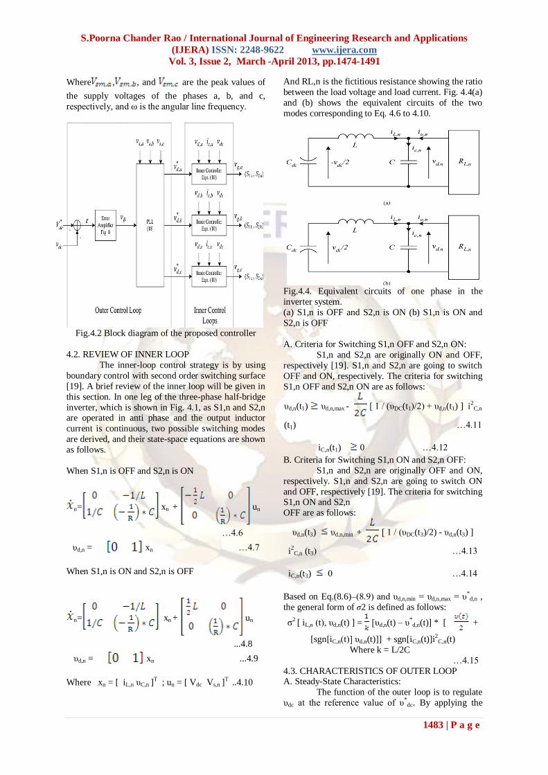
Fig.4.2 Block diagram of the proposed controller

4.2. REVIEW OF INNER LOOP

The inner-loop control strategy is by using

boundary control with second order switching surface

[19]. A brief review of the inner loop will be given in

this section. In one leg of the three-phase half-bridge

inverter, which is shown in Fig. 4.1, as S1,n and S2,n are operated in anti phase and the output inductor

current is continuous, two possible switching modes

are derived, and their state-space equations are shown

as follows.

When S1,n is OFF and S2,n is ON

n= xn + un

…4.6

υd,n = xn …4.7

When S1,n is ON and S2,n is OFF

n= xn + un

...4.8

υd,n = xn ...4.9

Where xn = [ iL,n υC,n ]T ; un = [ Vdc Vs,n ]

T ..4.10

And RL,n is the fictitious resistance showing the ratio

between the load voltage and load current. Fig. 4.4(a)

and (b) shows the equivalent circuits of the two

modes corresponding to Eq. 4.6 to 4.10.

Fig.4.4. Equivalent circuits of one phase in the

inverter system.

(a) S1,n is OFF and S2,n is ON (b) S1,n is ON and

S2,n is OFF

A. Criteria for Switching S1,n OFF and S2,n ON:

S1,n and S2,n are originally ON and OFF,

respectively [19]. S1,n and S2,n are going to switch

OFF and ON, respectively. The criteria for switching

S1,n OFF and S2,n ON are as follows:

υd,n(t1) υd,n,max - [ 1 / (υDC(t1)/2) + υd,n(t1) ] i2

C,n

(t1) …4.11

iC,n(t1) 0 …4.12

B. Criteria for Switching S1,n ON and S2,n OFF:

S1,n and S2,n are originally OFF and ON,

respectively. S1,n and S2,n are going to switch ON

and OFF, respectively [19]. The criteria for switching S1,n ON and S2,n

OFF are as follows:

υd,n(t3) υd,n,min + [ 1 / (υDC(t3)/2) - υd,n(t3) ]

i2C,n (t3) …4.13

iC,n(t3) 0 …4.14

Based on Eq.(8.6)–(8.9) and υd,n,min = υd,n,max = υ*d,n ,

the general form of σ2 is defined as follows:

σ2 [ iL,n (t), υd,n(t) ] = [υd,n(t) – υ*

d,n(t)] * [ +

[sgn[iC,n(t)] υd,n(t)]] + sgn[iC,n(t)]i2

C,n(t)

Where k = L/2C

…4.15

4.3. CHARACTERISTICS OF OUTER LOOP A. Steady-State Characteristics:

The function of the outer loop is to regulate

υdc at the reference value of υ*dc. By applying the




1484 | P a g e

conservation of energy, the DVR will ideally have

zero-average real power flow at the steady state.

Ps,a + Ps,b+ Ps,c = Po,a + Po,b + Po,c …4.16

Pa = Pb = Pc = 0 …4.17

Ps,n = υs,n io,n cos (θn - β) …4.18

Po,n = υo,n io,n cos (θn) ; Pn = υd,n io,n cos(υn) …4.19

where , , and are the input, output

powers, and power transferred of the each phase,

respectively, is the load current of each phase,

is the phase angle between and , β is the

phase angle between and , and is the

phase angle between and . Under supply-

voltage interruption, the outer loop will adjust the

value of β. The DVR will generate the required

magnitude and phase of in each phase

individually. The DVR will then absorb (deliver)

electric energy from (to) the dc link. As the

adjustment of β is common to the three phases, the

sagged phase(s) will be supported by the capacitor

bank and the un sagged phase(s). The corresponding

equations of are as follows:

υo,a (t) = Vom,a cos(ωt - β) …4.20

υo,b (t) = Vom,b cos(ωt - 120˚ - β) …4.21

υo,c (t) = Vom,c cos(ωt + 120˚ - β) …4.22

Where is the peak load voltage of phase n.

Fig. 4.3 shows the steady-state phasor

diagrams with one-phase sagged and three-phase

voltage balancing, respectively. The parameters used

are based on Tables 4.1-4.3. In Fig. 4.3(a), is

reduced to 120 V, while the other phases are at the

nominal value of 220 V. By increasing the value of β,

is established by the DVR and can be kept

at 220 V. Thus, part of the energy supplied to phase-a

load is supported by phase’s b and c.

In Fig. 4.3(b), all three phases are

unbalanced, where = 210 V, = 190 V, and

= 240 V. Again, by adjusting the value of β,

, , and are regulated at 220 V. For the phase

transformation between β and

α = - (β – υn- θn)

…4.23

Where is the phase difference between

and .

Based on Fig. 4.3(a) and by using Equations (4.19) to

(4.23), it can be shown that the steady-state power-

transfer equation can be expressed as follows:

…4.24

Detailed derivation of (34) is given in the

Appendix. The values of , ,

, and

are different in each phase. Thus, the power flow of

each phase inverter is different. β is controlled by the

outer loop in order to achieve power equilibrium in the system, and thus, satisfy eq.4.16 and 4.17.

TABLE 4.1 SPECIFICATIONS OF THE DVR

TABLE 4.2 PARAMETERS OF THE PLL AND

TRANSDUCER GAINS




1485 | P a g e

TABLE 4.3 COMPONENT VALUES OF THE DVR

B. Small Signal Modeling:

Fig. 4.5 shows the small-signal model of the

outer loop. It consists of the transfer characteristics of

the inner loop, inverter, PLL, and power-flow

controller. As the inner loop has much faster dynamic response than the outer loop, the small-signal transfer

function of the inner loop is unity. The transfer

function of the inverter describes the small-signal

behaviors between β and Vdc. The functional blocks

of power stage and controller are derived as follows.

Fig.4.5. Small-signal model of the outer loop

1) Relationship Between and : The small-

signal dclink voltage to dc-power-transfer function

Tp (s) is as follows:

…4.25

Where is the steady-state values of .

2) Relationship between Power Flow and the Phase

of With Respect to io,n in Each Phase: The

small-signal DVR phase- to-power transfer function

Tr,n (s)

…4.26

Where Vd is the steady-state values of vd .

3) Phase Transformation Between β and υ in Each

Phase: The transfer function Tpt,n (s) representing

the transformation between β and υ is

...4.27

Where Vs , Vo , and B are the steady-state values of

vs , vo , and β, respectively.

4) Phase Transformation Between β and vdc in

Inverter: The transfer function Tinv (s) of the inverter

is as follows [19]–[22]:

Tinv

=

...4.28

Fig.4.6. Circuit schematic of the power-flow

controller

5) PLL: The PLL consists of three components,

including the phase detector (PD), loop filter (LF),

and the voltage controlled oscillator (VCO)

[27].Based on the small-signal model of the PLL is as follows:

…4.29

Where A = - (Rl / (RcKpd)) ; ξ = 0.5 (

τKpdKlKvco) ; ωn = (KpdKlKvco/τ) …4.30

, , are the constant gains of PD, LF and

VCO, respectively.




1486 | P a g e

1. Power-Flow Controller:

The function of the power-flow controller is

to regulate vdc at the reference voltage Vdc, which

is determined by the voltage ratings of the capacitor and the switches. Charging or discharging the

capacitor Cdc is achieved by adjusting υn in three

phases individually. The regulation action is

performed by the error amplifier shown in Fig. 4.6.

The transfer function TC (s) can be shown in

(Eq.4.29-4.30), at the bottom of the page.

4.4. SIMPLIFIED DESIGN PROCEDURES:

The values of L, C, and Cdc in the inverter,

R1 , R2 , C1 , and C2 in the power-flow controller

are designed as follows.

A. Design of L and C in the Inverter:

The values of L and C in the output filters

are determined by considering the maximum voltage

drop across the inductor vL, D at the maximum line

current Io, max, angular line frequency ω, maximum

ripple current I ripple , and angular switching

frequency ωsw . As most of the load current is

designed to flow through L, the value of L is

determined by considering that its voltage drop vL, D

is small at the maximum line current Io, max.

Thus ωLIo,max < υL,D = L < (υL,D/ωIo,max) …4.31a

As the inverter output consists of high-frequency

harmonics, the fundamental component of the ripple

current through the filter is designed to be less than I

ripple. For the sake of simplicity In the calculation,

the load impedance at the switching frequency is

assumed to be infinite.

Thus

…4.31(b)

The nominal switching frequency is chosen

to be a few hundred times the line frequency. vL,D is

chosen to be 1% of the line voltage, and Iripple is

chosen to one half of the peak of the line current. As

shown in Table I, ωsw = 300 ω, vL,D = 2 V, and

Iripple = 2.6 A for the designed prototype. Based on

(Eq.4.31) and stated criteria, the values of L and C in

the output filters are determined.

B. Design of Cdc in the Inverter: The value of Cdc is determined by

…4.32

Where vo, nor and vs, min are nominal

value of load voltage and minimum voltage of supply

voltage in specification, respectively, tres is duration of restoration.

C. Design of R1 , R2 , C1 , and C2 in the Power-

Flow Controller:

The pole and zeros are designed as follows:

log ωp = Log ωz2 – (ψ/20) …4.33

Typically, ψ = 20 is chosen, and the ratio of

ωz1 and ωz2 is chosen to be at least 100, in order to

avoid overlapping in the two zeros.

Therefore

log ωz = log ω2z – 2 …4.34

Based on Eq. (4.35)–(4.37), R1 , R2 , C1 , and C2 are

designed by putting a value into one of them. The

practical simulation model of DVR is shown in Fig

4.9. The loop gain TOL(s), it is based on the

specifications and designed component values listed

in Tables 4.2 and 4.3. The bode plot shows operation

range, the frequency between ωcross, min, and

ωcross, max within the stable regions. Based on Eq.

(4.30), we have

ωz1 + ωz1 = (1/R2C2) + (1/R2C1) + (1/R1C2) …4.35

ωz1* ωz1 = (1/R1 R2 C1 C2) …4.36

ωP = (C1 + C2)/(C1 C2 R1 ) …4.37

4.5 Result Analysis Of A Fast Dynamic Control

Scheme For Capacitor-Supported Interline Dynamic

Voltage Restorer

4.5.1. Harmonic Distortions:

When large amount of loads are added or

removed at the load centre’s a dip in voltage level will take place and that can abrupt performance of the

customer’s equipment. The above mentioned are two

major power quality issues that existing in the power

systems. Due these effects the total harmonic

distortion that is transmitted in the line is 33.54% for

one complete cycle of the waveform and the

transmitted signals will affect the performance of the

line as shown in the fig.4.7.




1487 | P a g e

Fig. 4.7 The voltage and harmonic analysis of

waveform without DVR

Fig.4.8 Simulation model without DVR

When large amount of loads are connected

the dip in voltage will rise which can be reduced by

using a dynamic voltage restorer. The sag that is

reduced by using the DVR is shown in the below

fig.4.9. The storage element in the DVR i.e. capacitor

stored energy will be used to bounce back the sagged

phases to nominal values and the total harmonic distortion can be reduce to1.37% from a value

33.54% as shown in fig 4.9.

Fig.4.9 The voltage and harmonic analysis of

waveform with DVR

The voltage sag and swell cases that are compensated

by the dynamic voltage restorer are shown in the fig.

(4.11-4.14)

4.5.1. Voltage Sag:

The voltage sag effected on single and three phase conditions are shown in the fig.4.11-4.12

where the supply voltage is reduced from a value of

Vs=220V rms to 120V rms i.e. the percentage of sag

that resulted is around 45%. When a sag occurs in the

voltage then outer control loop and inner control loop

will initiate to release the energy stored in the

capacitor to restore the supply voltage to nominal

value. The voltage sag is compensated with the

transition time 250µsec to 180µsec.

4.5.2. Voltage Swell: The voltage swell effected on single and

three phase conditions are shown in the fig.4.13-4.14

where the supply voltage is increased from a value of

Vs=220V rms to 260V rms i.e. the percentage of

swell that resulted is around 19%. When a voltage

swell occurs in the voltage then outer control loop

and inner control loop will initiate to charge the

capacitor to restore the supply voltage to nominal

value. The voltage swell is compensated with the

transition time of 180µsec.

The dynamic voltage restorer provides the

compensation to the harmonics contents, voltage sag and voltage swell cases.




1488 | P a g e

Fig.4.11 Waveforms at three sagged phases under

condition. Vs,a , Vs,b , and Vs,c are changed from 220 to 120

Vrms .

Fig.4.12 Waveforms at single phase sagged

condition: Vs,a is changed from 220Vrms to 120Vrms.




1489 | P a g e

Fig.4.13 Waveforms at single phase swell condition.

Vs,a is changed from 220Vrms to 260V Vrms

Fig.4.14 Waveforms at three swell conditions. (a) Vs,a

, Vs,b , and Vs,c are changed from 220Vrms to 260Vrms.

4.6. COMPARISION OF RESULTS WITH AND

WITHOUT DVR:

The effect of voltage sag and swell has a

greater impact on the power that is transmitted from

sending end to recieveing end. The real power that is




1490 | P a g e

transmitted gets varied due to the addition of more

non-linear loads or sudden shutdown of large rating

loads. The voltage sag and swell cases cause

customer appliances to get abrupt by reducing their life span. The power quality at the load centre are

mostly electonic switched ones, so due to the

switching actions of these non-linear loads the level

of harmonics injected into the supply will be more

and the cost of the capacitors required to compensate

the harmonics will increase there by increasing the

overall cost.

When an automatically controlled regulators

are used then the chances of overcoming the voltage

sag or swell cases can be aoided. The dynamic

voltage restorer operates at desired levels to regulate voltages as well as eliminates the harmonics. The

entire mechanism uses capacitor banks to restore the

voltage to nominal values and the energy stored in

the capacitor can be charged from the supply it self.

Under normal operated conditions the MOSFET

switches which operate at 10 KHz frequency nor

inject nor charge the capacitor. When a voltage sag

occur the stored enrgy restores the voltage to nominal

value by discharging the energy. When a voltage

swell occur in any of the phases, the capacitor uses

the swelled phase to charge its energy to bounce to

normal full capacity. The total harmonic content that will be

available when a power system is operated under

sagged condition will be 33.54% i.e without using the

DVR. When a DVR is used in to back up the sagged

voltage to nominal value it also eliminates the total

harmonic content to a lower value lessthan 6%.

IV. CONCLUSION A control scheme for three-phase capacitor-supported interline DVR has been presented. By

integrating a recently proposed boundary-control

method with second-order switching surface (inner

loop), the dynamic response has been minimized to

two switching actions. The voltage sag, swell, and

voltage harmonic distortion have been compensated

by this DVR. Moreover, by using series bidirectional

inverter as DVR, capacitor banks are used to support

the dc link and the sagged phase(s) could be

supported by the un sagged phase(s). Long-duration

voltage sags and swell and three-phase voltage unbalance could be overcome by the proposed

power-flow controller (outer loop). The MOSFET

switches that are used in the voltage source converter

operate at a variable frequency range i.e. 10 KHz.

This has facilitated for the fast switching action and

provides dynamic response in turn maintains the

stability of the system. The designed model of

dynamic voltage restorer also reduces the harmonic

percentages that resulted due to MOSFET switching

actions. The gating pulse to the switch is generated

by the pulse width modulation technique. The

method has been verified with a review model. The

performances of the DVR have been demonstrated

and evaluated with different power-quality

disturbances. Experimental measurements are

favorably verified with theoretical results. The power quality problem issues related to voltage sag and

swell as well as total harmonic distortion can be

compensated effectively by using the dynamic

voltage restorer.

REFERENCES [1] M. Bollen, Understanding Power Quality

Problems, Voltage Sags and Interruptions.

New York: IEEE Press, 2000. [2] M. Sullivan, T. Vardell, and M. Johnson,

―Power interruption costs to industrial and

commercial consumers of electricity,‖ IEEE

Trans. Ind. App., vol. 33, no. 6, pp. 1448–

1458, Nov. 1997.

[3] N. Woodley, L. Morgan, and A. Sundaram,

―Experience with an inverterbased dynamic

voltage restorer,‖ IEEE Trans. Power Del.,

vol. 14, no. 3, pp. 1181–1186, Jul. 1999.

[4] R. R. Errabelli, Y. Y. Kolhatkar, and S. P. Das,

―Experimental investigation of DVRwith slidingmode control,‖ in Proc. IEEE Power

India Conf., Apr. 2006, paper 117.

[5] S. Lee, H. Kim, and S. K. Sul, ―A novel

control method for the compensation voltages

in dynamic voltage restorers,‖ in Proc. IEEE

APEC 2004, vol. 1, pp. 614–620.

[6] G. Joos, S. Chen, and L. Lopes, ―Closed-loop

state variable control of dynamic voltage

restorers with fast compensation

characteristics,‖ in Proc. IEEE IAS 2004, Oct.,

vol. 4, pp. 2252–2258.

[7] P.Ruilin and Z.Yuegen, ―Sliding mode control strategy of dynamic voltage restorer,‖ in Proc.

ICIECA 2005, Nov./Dec., p. 3.

[8] T. Jauch, A. Kara, M. Rahmani, and D.

Westermann, ―Power quality ensured by

dynamic voltage correction,‖ ABB Rev., vol. 4,

1998, pp. 25–36.

[9] C.S.Chang, S.W.Yang, and Y. S. Ho,

―Simulation and analysis of series voltage

restorer (SVR) for voltage sag relief,‖ in Proc.

IEEE PES Winter Meeting, Jan, 2000, vol. 4,

pp. 2476–2481. [10] C. Meyer, R. W. De Doncker, Y. W. Li, and F.

Blaabjerg, ―Optimized control strategy for a

medium-voltage DVR—Theoretical

investigations and experimental results,‖ IEEE

Trans. Power Electron., vol. 23, no. 6, pp.

2746–2754, Nov. 2008.

[11] S. S. Choi, B. H. Li, and D. M. Vilathgamuwa,

―Dynamic voltage regulation with minimum

energy injection,‖ IEEE Trans. Power Syst.,

vol. 15, no. 1, pp. 51–57, Feb. 2000.

[12] D. M. Vilathgamuwa, A. A. D. R. Perera, and

S. S. Choi, ―Voltage sag compensation with




1491 | P a g e

energy optimized dynamic voltage restorer,‖

IEEE Trans. Power Del., vol. 18, no. 3, pp.

928–936, Jul. 2003.

[13] K. Piatek, ―A new approach of DVR control with minimized energy injection,‖ in Proc.

PEMC2006, Aug., pp. 1490–1495.

[14] D. M. Vilathgamuwa, H.M.Wijekoon, and S.

S. Choi, ―Interline dynamic voltage restorer: A

novel and economical approach for multiline

power quality compensation,‖ IEEE Trans.

Ind. Appl., vol. 40, no. 6, pp. 1678– 1685,

Nov./Dec. 2004.

[15] D. Vilathgamuwa, H.M.Wijekoon, and S. S.

Choi, ―A novel technique to compensate

voltage sags in multiline distribution system—The interline dynamic voltage restorer,‖ IEEE

Trans. Ind. Electron., vol. 53, no. 5, pp. 1603–

1611, Oct. 2006.

[16] R. J. Nelson and D. G. Ramey, ―Dynamic

power and voltage regulator for an ac

transmission line,‖ U.S. Patent 5 610 501,

Mar. 1997. [17] A. van Zyl, R. Spee, A.

Faveluke, and S. Bhowmik, ―Voltage sag

ridethrough for adjustable-speed drives with

active rectifiers,‖ IEEE Trans. Ind. Appl., vol.

34, no. 6, pp. 1270–1277, Nov./Dec. 1998.

[18] A. Ghosh, A. K. Jindal, and A. Joshi, ―Design of a capacitor-supported dynamic voltage

restorer (DVR) for unbalanced and distorted

loads,‖ IEEE Trans. Power Del., vol. 19, no. 1,

pp. 405–413, Jan. 2004.

[19] C. Ho, H. Chung, and K. Au, ―Design and

implementation of a fast dynamic control

scheme for capacitor-supported dynamic

voltage restorers,‖ IEEE Trans. Power

Electron., vol. 23, no. 1, pp. 237–251, Jan.

2008.

[20] K. Leung and H. Chung, ―Derivation of a second-order switching surface in the

boundary control of buck converters,‖ IEEE

Power Electron. Lett., vol. 2, no. 2, pp. 63–67,

Jun. 2004.

[21] K. Leung and H. Chung, ―A comparative study

of the boundary control of buck converters

using first- and second-order switching

surfaces,‖ IEEE Trans. Power Electron., vol.

22, no. 4, pp. 1196–1209, Jul. 2007.

[22] D. O. Koval and M. B. Hughes, ―Canadian

national power quality survey: Frequency of industrial and commercial voltage sags,‖ IEEE

Trans. Ind. Appl., vol. 33, no. 3, pp. 622–627,

May/Jun. 1997.

[23] A. El Mofty and K. Youssef, ―Industrial power

quality problems,‖ in Proc. IEE Conf. Electr.

Distrib., Part 1: Contrib., Jun. 2001, vol. 2,

pp. 139–139.

[24] E. W. Gunther and H. Mebta, ―A survey of

distribution system power quality—

Preliminary results,‖ IEEE Trans. Power Del.,

vol. 10, no. 1, pp. 322–329, Jan. 1995.

[25] M. H. J. Bollen, ―Voltage sags: Effects,

mitigation and prediction,‖ Power Eng. J., vol. 10, no. 3, pp. 129–135, Jun. 1996.

[26] B. M. Weedy and B. J. Cory, Electric Power

System, 4th ed. New York: Wiley, 1998.

[27] H. M. Berlin, Design of Phase-Locked Loop

Circuits with Experiments, 1st ed.

Indianapolis, IN: Sams, 1985.

[28] H. Kim and S. K. Sul, ―Compensation voltage

control in dynamic voltage restorers by use of

feed forward and state feedback scheme,‖

IEEE Trans. Power Electron., vol. 20, no. 5,

pp. 1169–1176, Jan. 2005. [29] B.Wang, G.Venkataramanan, and M. Illindala,

―Operation and control of a dynamic voltage

restorer using transformer coupled H-bridge

converters,‖ IEEE Trans. Power Electron.,

vol. 21, no. 4, pp. 1053–1061, Jun. 2006.

[30] H. Awad, J. Svensson, and M Bollen,

―Mitigation of unbalanced voltage dips using

static series compensator,‖ IEEE Trans. Power

Electron., vol. 19, no. 3, pp. 837–846, May

2004.

[31] Y. Chiu,K. Leung, andH.Chung, ―High-order

switching surface in boundary control of inverters,‖ IEEE Trans. Power Electron., vol.

22, no. 5, pp. 1753–1765, Sep. 2007.

[32] M. Ordonez, J. E. Quaicoe, and M. T. Iqbal,

―Advanced boundary control of inverters using

the natural switching surface: Normalized

geometrical derivation,‖ IEEE Trans. Power

Electron., vol. 23, no. 6, pp. 2915–2930, Nov.

2008.

[33] S. Chen, Y. M. Lai, S. C. Tan, and C. K. Tse,

―Boundary control with ripple-derived

switching surface for DC–AC inverters,‖ IEEE Trans. Power Electron., vol. 24, no. 12, pp.

2873–2885, Dec. 2009.

[34] M. Rashid, Power Electronics, Circuits,

Devices, and Applications, 3rd ed. Englewood

Cliffs, NJ: Prentice-Hall, 2004.]

[35] C. Ho, K. Au, and H. Chung, ―Digital

implementation of boundary control with

second-order switching surface,‖ in Proc.

IEEE PESC2007, Jun., pp. 1658–1664

applications and extensions.

ih3214741491

Documents

load voltage

voltage swell

voltage sags

injecting voltage

dynamic voltage restorationdvr

dynamic voltage restorer

sagged supply voltage

supply voltage stays