ill–posed inverse problems in image processing · ill–posed inverse problems in image...
TRANSCRIPT

Ill–Posed Inverse Problems in Image ProcessingIntroduction, Structured matrices, Spectral filtering,
Regularization, Noise revealing
I. Hnetynkova1 , M. Plesinger2, Z. Strakos3
[email protected], [email protected], [email protected]
1,3Faculty of Mathematics and Phycics, Charles University, Prague2Seminar of Applied Mathematics, Dept. of Math., ETH Zurich
1,2,3Institute of Computer Science, Academy of Sciences of the Czech Republic
SNA ’11, January 24—28
1 / 57

Motivation. A gentle start ...What is it an inverse problem?
2 / 57

Motivation. A gentle start ...What is it an inverse problem?
Forward problem
Inverse problem
[Kjøller: M.Sc. thesis, DTU Lyngby, 2007].
observation b unknown xA(x) = b
A
A−1
2/ 57
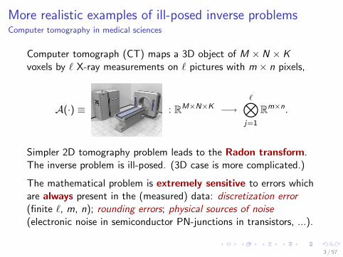
More realistic examples of ill-posed inverse problemsComputer tomography in medical sciences
Computer tomograph (CT) maps a 3D object of M × N × Kvoxels by � X-ray measurements on � pictures with m × n pixels,
A(·) ≡ : RM×N×K −→
�⊗j=1
Rm×n.
Simpler 2D tomography problem leads to the Radon transform.The inverse problem is ill-posed. (3D case is more complicated.)
The mathematical problem is extremely sensitive to errors whichare always present in the (measured) data: discretization error(finite �, m, n); rounding errors; physical sources of noise(electronic noise in semiconductor PN-junctions in transistors, ...).
3 / 57

More realistic examples of ill-posed inverse problemsTransmision computer tomography in crystalographics
Reconstruction of an unknown orientation distribution function(ODF) of grains in a given sample of a polycrystalline matherial,
A
⎛⎜⎜⎝
⎞⎟⎟⎠ ≡ −→
⎛⎜⎜⎝ , . . .
⎞⎟⎟⎠
︸ ︷︷ ︸observation = data +noise
.
The right-hand side is a set of measured difractograms.[Hansen, Sørensen, Sudkosd, Poulsen: SIIMS, 2009].
Further analogous applications also in geology, e.g.:
� Seismic tomography (cracks in tectonic plates),
� Gravimetry & magnetometry (ore mineralization).
4 / 57

More realistic examples of ill-posed inverse problemsImage deblurring—Our pilot application
Our pilot application is the image deblurring problem
A
⎛⎜⎜⎜⎝
x = true image ⎞⎟⎟⎟⎠ −→
b = blurred, noisy image
= data + noise.
It leads to a linear system Ax = b with square nonsingular matrix.Let us motivate our tutorial by a “naive solution” of this system
A−1
⎛⎜⎜⎜⎝
b = blurred, noisy image ⎞⎟⎟⎟⎠ =
x = inverse solution
.
[Nagy: Emory University].
5 / 57

More realistic examples of ill-posed inverse problemsGeneral framework
In general we deal with a linear problem
Ax = b
which typically arose as a discretization of a
Fredholm integral equation of the 1st kind
y(s) =
∫K (s, t)x(t)dt.
The observation vector (right-hand side) is contaminated by noise
b = bexact + bnoise, where ‖bexact‖ � ‖bnoise‖.
6 / 57

More realistic examples of ill-posed inverse problemsGeneral framework
We want to compute (approximate)
xexact ≡ A−1bexact.
Unfortunatelly, because the problem is inverse and ill-posed
‖A−1bexact‖ � ‖A−1bnoise‖,
the data we look for are in the naive solution covered by theinverted noise. The naive solution
x = A−1b = A−1bexact + A−1bnoise
typically has nothing to do with the wanted xexact.
7 / 57

Outline of the tutorial
� Lecture I—Problem formulation:
Mathematical model of blurring, System of linear algebraicequations, Properties of the problem, Impact of noise.
� Lecture II—Regularization:
Basic regularization techniques (TSVD, Tikhonov), Criteriafor choosing regularization parameters, Iterativeregularization, Hybrid methods.
� Lecture III—Noise revealing:
Golub-Kahan iteratie bidiagonalization and its properties,Propagation of noise, Determination of the noise level, Noisevector approximation, Open problems.
8 / 57
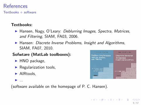
ReferencesTextbooks + software
Textbooks:
� Hansen, Nagy, O’Leary: Deblurring Images, Spectra, Matrices,and Filtering, SIAM, FA03, 2006.
� Hansen: Discrete Inverse Problems, Insight and Algorithms,SIAM, FA07, 2010.
Sofwtare (MatLab toolboxes):
� HNO package,
� Regularization tools,
� AIRtools,
� ...
(software available on the homepage of P. C. Hansen).
9 / 57

Outline of Lecture I
� 1. Mathematical model of blurring:
Blurring as an operator on the vector space of matrices,Linear and spatial invariant operator, Point-spread-function,2D convolution, Boundary conditions.
� 2. System of linear algebraic equations:
Gaußian blur, Exploiting the separability, 1D Gaußian blurringoperator, Boundary conditions, 2D Gaußian blurring operator,Structured matrices.
� 3. Properties of the problem:
Smoothing properties, Singular vectors of A, Singular valuesof A, The right-hand side, Discrete Picard condition (DPC),SVD and Image deblurring problem, Singular images.
� 4. Impact of noise:
Violation of DPC, Naive solution, Regularization and filtering.
10 / 57

1. Mathematical model of blurring
11 / 57

1. Mathematical model of blurringBlurring as an operator of the vector space of images
The grayscale image can be considered as a matrix, consider forconvenience black ≡ 0 and white ≡ 1.
Consider a, so called, single-pixel-image (SPI) and a blurringoperator as follows
A(X ) = A
⎛⎜⎜⎝
⎞⎟⎟⎠ = = B ,
where X = [x1, . . . , xk ], B = [b1, . . . , bk ] ∈ Rk×k .
The image (matrix) B is called point-spread-function (PSF).
(In Parts 1, 2, 3 we talk about the operator, the right-hand side is noise-free.)
12 / 57

1. Mathematical model of blurringLinear and spatial invariant operator
Consider A to be:
1. linear (additive & homogenous),
2. spatial invariant.
Linearity of A allows to rewrite A(X ) = B as a system of linearalgebraic equations
Ax = b, A ∈ RN×N , x , b ∈ R
N .
(We do not know how, yet.)
13 / 57

1. Mathematical model of blurringLinear and spatial invariant operator
The matrix X containing the SPI has only one nonzero entry(moreover equal to one).
Therefore the unfolded X
x = vec(X ) = [xT1 , . . . , xT
k ]T = ej
represents an Euclidean vector.
The unfolding of the corredponding B (containing the PSF) thenrepresents jth column of A
A ej = b = vec(B) = [bT1 , . . . , bT
k ]T .
The matrix A is composed columnwise by unfolded PSFscorresponding to SPIs with different positions of the nonzero pixel.
14 / 57

1. Mathematical model of blurringLinear and spatial invariant operator
Spatial invariance of A ≡ The PSF is the same for all positi-ons of the nonzero pixel in SPI. (What about pixels close to theborder?)Linearity + spatial invariance:
↓ ↓ ↓ ↓ ↓ ↓
+ + + + =
+ + + + =
First row: Original (SPI) images (matrices X ).Second row: Blurred (PSF) images (matrices B = A(X )).
15 / 57

1. Mathematical model of blurringPoint—spread—function (PSF)
Linear and spatially invariant blurring operator A is fully describedby its action on one SPI, i.e. by one PSF. (Which one?)
Recall: Up to now the width and height of both the SPI and PSFimages have been equal to some k, called the window size.
For correctness the window size must be properly chosen, namely:
� the window size must be sufficiently large
(increase of k leads to extension of PSF image by black),
� the window is typically square (for simplicity),
� we use window of odd size (for simplicity), i.e.
k = 2� + 1.
16 / 57
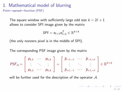
1. Mathematical model of blurringPoint—spread—function (PSF)
The square window with sufficiently large odd size k = 2� + 1allows to consider SPI image given by the matrix
SPI = e�+1eT�+1 ∈ R
k×k
(the only nonzero pixel is in the middle of SPI).
The corresponding PSF image given by the matrix
PSFA =
⎡⎢⎣
p1,1 · · · p1,k...
. . ....
pk,1 · · · pk,k
⎤⎥⎦ =
⎡⎢⎣
p−�,−� · · · p−�,+�...
. . ....
p+�,−� · · · p+�,+�
⎤⎥⎦ ∈ R
k×k
will be further used for the description of the operator A.
17 / 57

1. Mathematical model of blurringPoint—spread—function (PSF)
Examples of PSFA:
horizontal vertical out-of-focus Gaußianmotion blur motion blur blur blur
18 / 57

1. Mathematical model of blurring2D convolution
We have the linear, spatial invariant A given by PSFA ∈ Rk×k .
Consider a general grayscale image given by a matrix X ∈ Rm×n.
How to realize the action of A on X , i.e. B = A(X ), using PSFA?
Entrywise application of PSF:
1. X =∑m
i=1
∑nj=1 Xi ,j , where Xi ,j ≡ xi ,j(ei e
Tj ) ∈ R
m×n;
2. realize the action of A on the single-pixel-image Xi ,j
Xi ,j =
⎡⎣ 0 0 0
0 xi ,jSPI 0
0 0 0
⎤⎦ −→ Bi ,j ≡
⎡⎣ 0 0 0
0 xi ,jPSFA 0
0 0 0
⎤⎦ ;
3. B =∑m
i=1
∑nj=1 Bi ,j due to the linearity of A.
19 / 57

1. Mathematical model of blurring2D convolution
5-by-5 example: B =∑m
i=1
∑nj=1 Bi ,j = x1,1( ) + . . . + x1,5( )
+x2,1( ) +x2,2
⎛⎜⎝
0 0 0 0 00 0 0 0 0
p3,1 p3,2 p3,3 0 0p2,1 p2,2 p2,3 0 0p1,1 p1,2 p1,3 0 0 ⎞
⎟⎠+x2,3
⎛⎜⎝
0 0 0 0 00 0 0 0 00 p3,1 p3,2 p3,3 00 p2,1 p2,2 p2,3 00 p1,1 p1,2 p1,3 0 ⎞
⎟⎠+x2,4
⎛⎜⎝
0 0 0 0 00 0 0 0 00 0 p3,1 p3,2 p3,3
0 0 p2,1 p2,2 p2,3
0 0 p1,1 p1,2 p1,3⎞⎟⎠+x2,5( )
+x3,1( ) +x3,2
⎛⎜⎝
0 0 0 0 0p3,1 p3,2 p3,3 0 0p2,1 p2,2 p2,3 0 0p1,1 p1,2 p1,3 0 00 0 0 0 0 ⎞
⎟⎠+x3,3
⎛⎜⎝
0 0 0 0 00 p3,1 p3,2 p3,3 00 p2,1 p2,2 p3,3 00 p1,1 p1,2 p1,3 00 0 0 0 0 ⎞
⎟⎠+x3,4
⎛⎜⎝
0 0 0 0 00 0 p3,1 p3,2 p3,3
0 0 p2,1 p2,2 p2,3
0 0 p1,1 p1,2 p1,3
0 0 0 0 0 ⎞⎟⎠+x3,5( )
+x4,1( ) +x4,2
⎛⎜⎝
p3,1 p3,2 p3,3 0 0p2,1 p2,2 p2,3 0 0p1,1 p1,2 p1,3 0 00 0 0 0 00 0 0 0 0 ⎞
⎟⎠+x4,3
⎛⎜⎝
0 p3,1 p3,2 p3,3 00 p2,1 p2,2 p2,3 00 p1,1 p1,2 p1,3 00 0 0 0 00 0 0 0 0 ⎞
⎟⎠+x4,4
⎛⎜⎝
0 0 p3,1 p3,2 p3,3
0 0 p2,1 p2,2 p2,3
0 0 p1,1 p1,2 p1,3
0 0 0 0 00 0 0 0 0 ⎞
⎟⎠+x4,5( )
+x5,1( ) + . . . + x5,5( ), where
PSFA =
⎛⎝ p1,1 p1,2 p1,3
p2,1 p2,2 p2,3
p3,1 p3,2 p3,3
⎞⎠,
b3,3 = x2,2 p3,3 + x2,3 p3,2 + x2,4 p3,1
+ x3,2 p2,3 + x3,3 p2,2 + x3,4 p2,1
+ x4,2 p1,3 + x4,3 p1,2 + x4,4 p1,1
.
20 / 57
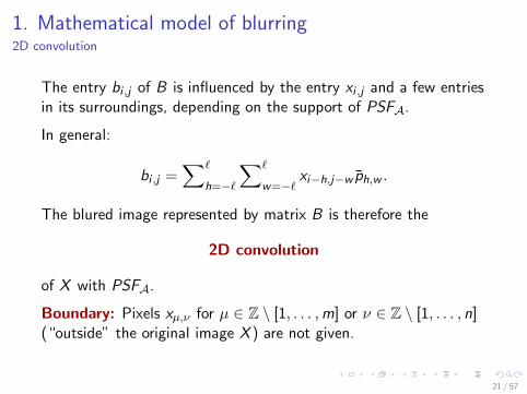
1. Mathematical model of blurring2D convolution
The entry bi ,j of B is influenced by the entry xi ,j and a few entriesin its surroundings, depending on the support of PSFA.
In general:
bi ,j =∑�
h=−�
∑�
w=−�xi−h,j−w ph,w .
The blured image represented by matrix B is therefore the
2D convolution
of X with PSFA.
Boundary: Pixels xμ,ν for μ ∈ Z \ [1, . . . ,m] or ν ∈ Z \ [1, . . . , n](“outside” the original image X ) are not given.
21 / 57

1. Mathematical model of blurringBoundary conditions (BC)
Real-world blurred image B is involved by the information whichis outside the scene X , i.e. by the boundary pixels xμ,ν .For the reconstruction of the real-world scene (deblurring) we dohave to consider some boundary condition:
� Outside the scene is nothing, xμ,ν = 0 (black), e.g., inastrononomical observations.
� The scene contains periodic patterns, e.g., inmicro/nanoscale imaging of matherials.
� The scene can be prolongated by reflecting.
Zero boundary Periodic boundary Reflexive boundary
22 / 57

1. Mathematical model of blurringSummary
Now we know “everything” about the simplest mathematicalmodel of blurring:
� We consider linear, spatial invariant operator A, which isrepresented by its point-spread-function PSFA.
� The 2D convolution of true scene with thepoint-spread-function represents the blurring.
� Convolution uses some information from the outside of thescene, therefore we need to consider some boundaryconditions.
23 / 57
2. System of linear algebraic equations
24 / 57

2. System of linear algebraic equationsBasic concept
The problem A(X ) = B can be rewritten (emploing the 2Dconvolution formula) as a system of linear algebraic equations
Ax = b, A ∈ Rmn×mn, x = vec(X ), b = vec(B) ∈ R
mn,
where the entries of A are the entries of the PSF, and
bi ,j =∑�
h=−�
∑�
w=−�xi−h,j−w ph,w .
In general:
� PSF has small localized support,
� each pixel is influenced only by a few pixels in its closesurroundings,
� therefore A is sparse.
25 / 57

2. System of linear algebraic equationsGaußian PSF / Gaußian blur
In the rest we consider Gaußian blur:
−4
−2
0
2
4
−4
−2
0
2
4
0
0.5
1
1.5
−3 −2 −1 0 1 2 3
0
0.5
1
1.5
Gaußian PSF G2D(h, w) G1D(ξ)
where (in a continuous domain)
G2D(h,w) = e−(h2+w2) = e−h2e−w2
, G1D(ξ) = e−ξ2.
Gaußian blur is the simplest and in many cases sufficient model.A big advantage is its separability G2D(h,w) = G1D(h)G1D(w).
26 / 57

2. System of linear algebraic equationsExploiting the separability
Consider the 2D convolution with Gaußian PSF in a continuousdomain. Exploiting the separability, we get
B(i , j) =
∫∫R2
X (i − h, j − w) e−(h2+w2) dh dw
=
∫ ∞
−∞
(∫ ∞
−∞X (i − h, j − w) e−h2
dh
)e−w2
dw
=
∫ ∞
−∞Y (i , j − w)e−w2
dw ,
where Y (i , j) =
∫ ∞
−∞X (i − h, j) e−h2
dh.
The blurring in the direction h (height) is independent on theblurring in the direction w (width).In the discrete setting: The blurring of columns of X isindependent on the blurring of rows of X .
27 / 57
2. System of linear algebraic equationsExploiting the separability
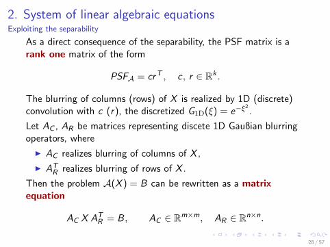
As a direct consequence of the separability, the PSF matrix is arank one matrix of the form
PSFA = crT , c , r ∈ Rk .
The blurring of columns (rows) of X is realized by 1D (discrete)convolution with c (r), the discretized G1D(ξ) = e−ξ2
.
Let AC , AR be matrices representing discete 1D Gaußian blurringoperators, where
� AC realizes blurring of columns of X ,
� ATR realizes blurring of rows of X .
Then the problem A(X ) = B can be rewritten as a matrixequation
AC X ATR = B , AC ∈ R
m×m, AR ∈ Rn×n.
28 / 57

2. System of linear algebraic equations1D convolution
Consider the following example of an AC related 1D convolution:
⎡⎢⎢⎢⎢⎢⎢⎣
β1
β2
β3
β4
β5
β6
⎤⎥⎥⎥⎥⎥⎥⎦
=
⎡⎢⎢⎢⎢⎢⎢⎣
c5 c4 c3 c2 c1
c5 c4 c3 c2 c1
c5 c4 c3 c2 c1
c5 c4 c3 c2 c1
c5 c4 c3 c2 c1
c5 c4 c3 c2 c1
⎤⎥⎥⎥⎥⎥⎥⎦
⎡⎢⎢⎢⎢⎢⎢⎢⎢⎢⎢⎢⎢⎢⎢⎢⎣
ξ−1
ξ0
ξ1
ξ2
ξ3
ξ4
ξ5
ξ6
ξ7
ξ8
⎤⎥⎥⎥⎥⎥⎥⎥⎥⎥⎥⎥⎥⎥⎥⎥⎦
,
where b = [β1, . . . , β6]T , x = [ξ1, . . . , ξ6]
T ,and c = [c1, . . . , c5]
T is the 1D (Gaußian) point-spread-function.
29 / 57

2. System of linear algebraic equationsBoundary conditions
The vector [ξ−1, ξ0|ξ1, . . . , ξ6|ξ7, ξ8]T represents the true scene. In
the reconstruction we consider:
[0, 0|ξ1, . . . , ξ6|0, 0]T ∼ zero boundary condition,
[ξ5, ξ6|ξ1, . . . , ξ6|ξ1, ξ2]T ∼ periodic boundary condition, or
[ξ2, ξ1|ξ1, . . . , ξ6|ξ6, ξ5]T ∼ reflexive boundary condition.
In general AC = M + BC , where
M =
⎡⎢⎢⎢⎢⎢⎢⎣
c3 c2 c1
c4 c3 c2 c1
c5 c4 c3 c2 c1
c5 c4 c3 c2 c1
c5 c4 c3 c2
c5 c4 c3
⎤⎥⎥⎥⎥⎥⎥⎦
,
and BC is a correction due to the boundary conditions.
30 / 57

2. System of linear algebraic equationsBoundary conditions
Zero boundary condition:
ACx=
⎡⎢⎢⎢⎢⎢⎢⎣
c5 c4 c3 c2 c1
c5 c4 c3 c2 c1
c5 c4 c3 c2 c1
c5 c4 c3 c2 c1
c5 c4 c3 c2 c1
c5 c4 c3 c2 c1
⎤⎥⎥⎥⎥⎥⎥⎦
⎡⎢⎢⎢⎢⎢⎢⎢⎢⎢⎢⎢⎢⎢⎢⎢⎣
00
ξ1
ξ2
ξ3
ξ4
ξ5
ξ6
00
⎤⎥⎥⎥⎥⎥⎥⎥⎥⎥⎥⎥⎥⎥⎥⎥⎦
=
⎡⎢⎢⎢⎢⎢⎢⎣
c3 c2 c1
c4 c3 c2 c1
c5 c4 c3 c2 c1
c5 c4 c3 c2 c1
c5 c4 c3 c2
c5 c4 c3
⎤⎥⎥⎥⎥⎥⎥⎦
⎡⎢⎢⎢⎢⎢⎢⎣
ξ1
ξ2
ξ3
ξ4
ξ5
ξ6
⎤⎥⎥⎥⎥⎥⎥⎦,
i.e. here BC = 0 and AC = M is a Toeplitz matrix.
31 / 57
2. System of linear algebraic equationsBoundary conditions
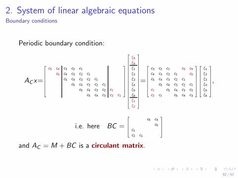
Periodic boundary condition:
ACx=
⎡⎢⎢⎢⎢⎢⎢⎣
c5 c4 c3 c2 c1
c5 c4 c3 c2 c1
c5 c4 c3 c2 c1
c5 c4 c3 c2 c1
c5 c4 c3 c2 c1
c5 c4 c3 c2 c1
⎤⎥⎥⎥⎥⎥⎥⎦
⎡⎢⎢⎢⎢⎢⎢⎢⎢⎢⎢⎢⎢⎢⎢⎢⎣
ξ5
ξ6
ξ1
ξ2
ξ3
ξ4
ξ5
ξ6
ξ1
ξ2
⎤⎥⎥⎥⎥⎥⎥⎥⎥⎥⎥⎥⎥⎥⎥⎥⎦
=
⎡⎢⎢⎢⎢⎢⎢⎣
c3 c2 c1 c5 c4
c4 c3 c2 c1 c5
c5 c4 c3 c2 c1
c5 c4 c3 c2 c1
c1 c5 c4 c3 c2
c2 c1 c5 c4 c3
⎤⎥⎥⎥⎥⎥⎥⎦
⎡⎢⎢⎢⎢⎢⎢⎣
ξ1
ξ2
ξ3
ξ4
ξ5
ξ6
⎤⎥⎥⎥⎥⎥⎥⎦,
i.e. here BC =
⎡⎢⎢⎣
c5 c4
c5
c1
c2 c1
⎤⎥⎥⎦
and AC = M + BC is a circulant matrix.
32 / 57

2. System of linear algebraic equationsBoundary conditions
Reflexive boundary condition:
ACx=
⎡⎢⎢⎢⎢⎢⎢⎣
c5 c4 c3 c2 c1
c5 c4 c3 c2 c1
c5 c4 c3 c2 c1
c5 c4 c3 c2 c1
c5 c4 c3 c2 c1
c5 c4 c3 c2 c1
⎤⎥⎥⎥⎥⎥⎥⎦
⎡⎢⎢⎢⎢⎢⎢⎢⎢⎢⎢⎢⎢⎢⎢⎢⎣
ξ2
ξ1
ξ1
ξ2
ξ3
ξ4
ξ5
ξ6
ξ6
ξ5
⎤⎥⎥⎥⎥⎥⎥⎥⎥⎥⎥⎥⎥⎥⎥⎥⎦
=
⎡⎢⎢⎢⎢⎢⎢⎣
c3+c4 c2+c5 c1
c4+c5 c3 c2 c1
c5 c4 c3 c2 c1
c5 c4 c3 c2 c1
c5 c4 c3 c2+c1
c5 c4+c1 c3+c2
⎤⎥⎥⎥⎥⎥⎥⎦
⎡⎢⎢⎢⎢⎢⎢⎣
ξ1
ξ2
ξ3
ξ4
ξ5
ξ6
⎤⎥⎥⎥⎥⎥⎥⎦,
i.e. here BC =
⎡⎢⎢⎣
c4 c5
c5
c1
c1 c2
⎤⎥⎥⎦
and AC = M + BC is a Toeplitz-plus-Hankel matrix.
33 / 57

2. System of linear algebraic equationsBoundary conditions—Summary
Three types of boundary conditions:
� zero boundary condition,
� periodic boundary condition,
� reflexive boundary condition,
correspond to the three types of matrices AC and AR :
� Toeplitz matrix,
� circulant matrix,
� Toeplitz-plus-Hankel matrix,
in the linear system of the form
AC X ATR = B .
34 / 57
2. System of linear algebraic equations2D Gaußian blurring operator—Kroneckerized product structure
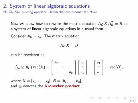
Now we show how to rewrite the matrix equation AC X ATR = B as
a system of linear algebraic equations in a usual form.
Consider AR = In. The matrix equation
AC X = B
can be rewritten as
(In ⊗ AC ) vec(X ) =
⎡⎢⎣
AC
. . .
AC
⎤⎥⎦
⎡⎢⎣
x1...xn
⎤⎥⎦ =
⎡⎢⎣
b1...
bn
⎤⎥⎦ = vec(B),
where X = [x1, . . . , xn], B = [b1, . . . , bn],and ⊗ denotes the Kronecker product.
35 / 57

2. System of linear algebraic equations2D Gaußian blurring operator—Kroneckerized product structure
Consider AC = Im. The matrix equation X ATR = B can be
rewritten as
(AR ⊗ Im) vec(X ) =
⎡⎢⎣
aR1,1Im · · · aR
1,nIm...
. . ....
aRn,1Im · · · aR
n,nIm
⎤⎥⎦
⎡⎢⎣
x1...xn
⎤⎥⎦ =
⎡⎢⎣
b1...
bn
⎤⎥⎦ = vec(B).
Consequently AC X ATR = (AC X )AT
R gives
(AR ⊗ Im)vec(AC X ) = (AR ⊗ Im)(In ⊗ AC )vec(X ).
Using properties of Kronecker product, this system is equivalent to
Ax = (AR ⊗ AC ) vec(X ) = vec(B) = b,
where
A =
⎡⎢⎣
aR1,1AC · · · aR
1,nAC...
. . ....
aRn,1AC · · · aR
n,nAC
⎤⎥⎦ ∈ R
mn×mn.
36 / 57

2. System of linear algebraic equationsStructured matrices
We have
A = AR ⊗ AC =
⎡⎢⎣
aR1,1AC · · · aR
1,nAC...
. . ....
aRn,1AC · · · aR
n,nAC
⎤⎥⎦ ∈ R
mn×mn,
where AC , AR are Toeplitz, circulant, or Toeplitz-plus-Hankel.
If AC is Toeplitz, then A is a matrix with Toeplitz blocks.
If AR is Toeplitz, then A is a block-Toeplitz matrix.
If AC and AR are Toeplitz (zero BC), then A is
block—Toeplitz with Toeplitz blocks (BTTB).
Analogously, for periodic BC we get BCCB matrix, for reflexie BCwe get a sum of four matrices BTTB+BTHB+BHTB+BHHB.
37 / 57

3. Properties of the problem
38 / 57

3. Properties of the problemSmoothing properties
We have an inverse ill-posed problem Ax = b, a discretization of aFredholm integral equation of the 1st kind
y(s) =
∫K (s, t)x(t)dt.
The matrix A is a restriction of the integral kernel K (s, t)(the convolution kernel in image deblurring)
� the kernel K (s, t) has smoothing property,
� therefore the vector y(s) is smooth,
and these properties are inherited by the discretized problem.Further analysis is based on the singular value decomposition
A = UΣV T , U ∈ RN×N , Σ ∈ R
N×N , V ∈ RN×N ,
(and N = mn in image deblurring).
39 / 57

3. Properties of the problemSingular vectors of A
Singular vectors of A represent bases with increasing frequencies:
0 200 400−0.1
0
0.1
u1
0 200 400−0.1
0
0.1
u2
0 200 400−0.1
0
0.1
u3
0 200 400−0.1
0
0.1
u4
0 200 400−0.1
0
0.1
u5
0 200 400−0.1
0
0.1
u6
0 200 400−0.1
0
0.1
u7
0 200 400−0.1
0
0.1
u8
0 200 400−0.1
0
0.1
u9
0 200 400−0.1
0
0.1
u10
0 200 400−0.1
0
0.1
u11
0 200 400−0.1
0
0.1
u12
First 12 left singular vectors of 1D ill-posed problem SHAW(400)[Regularization Toolbox].
40 / 57

3. Properties of the problemSingular values of A
Singular values decay without a noticeable gap (SHAW(400)):
0 2 4 6 8 10 12 14 16 18
10−10
10−8
10−6
10−4
10−2
100
102
j
sing
ular
val
ue σ
j
41 / 57

3. Properties of the problemThe right-hand side
First recall that b is the discretized smooth y(s), therefore
b is smooth, i.e. dominated by low frequencies.
Thus b has large components in directions of several first vectorsuj , and |uT
j b| on average decay with j .
42 / 57

3. Properties of the problemThe Discrete Picard condition
Using the dyadic form of SVD
A =∑N
j=1ujσjv
Tj , N is the dimension of the discretized K (s, t),
the solution of Ax = b can be rewritten as a linear combination ofright-singular vectors,
x = A−1b =∑N
j=1
uTj b
σjvj .
Since x is a discretization of some real-world object x(t)(e.g., an “true image”) the sequence of these sums converges tox(t) with N −→ ∞.
This is possible only if |uTj b| are on average decay faster than σj .
This property is called the (discrete) Picard condition (DPC).
43 / 57

3. Properties of the problemThe Discrete Picard condition
The discrete Picard condition (SHAW(400)):
0 10 20 30 40 50 60
10−40
10−30
10−20
10−10
100
singular value number
σj, double precision arithmetic
σj, high precision arithmetic
|(bexact, uj)|, high precision arithmetic
44 / 57

3. Properties of the problemSVD and Image deblurring problem
Back to the image deblurring problem: We have
AC X ATR = B ⇐⇒ (AR ⊗ AC ) vec(X ) = vec(B).
Consider SVDs of both AC and AR
AC = UC diag(sC )V TC , AR = UR diag(sR)V T
R ,
sC = [σC1 , . . . , σC
m]T ∈ Rm, sR = [σR
1 , . . . , σRn ]T ∈ R
n.
Using the basic properties of the Kronecker product
A = AR ⊗ AC = (UR diag(sR)V TR ) ⊗ (UC diag(sC )V T
C )
= (UR ⊗ UC )diag(sR ⊗ sC )(VR ⊗ VC )T = UΣV T ,
we get SVD of A (up to the ordering of singular values).
45 / 57
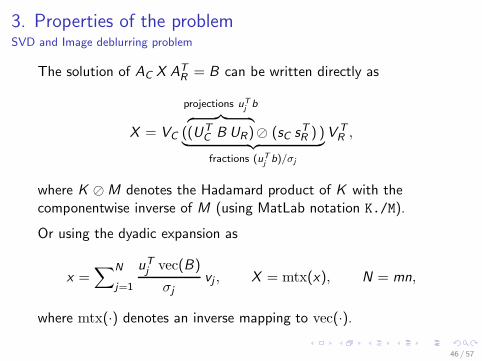
3. Properties of the problemSVD and Image deblurring problem
The solution of AC X ATR = B can be written directly as
X = VC (
projections uTj b︷ ︸︸ ︷
(UTC B UR)� (sC sT
R ) )︸ ︷︷ ︸fractions (uT
j b)/σj
V TR ,
where K � M denotes the Hadamard product of K with thecomponentwise inverse of M (using MatLab notation K./M).
Or using the dyadic expansion as
x =∑N
j=1
uTj vec(B)
σjvj , X = mtx(x), N = mn,
where mtx(·) denotes an inverse mapping to vec(·).
46 / 57

3. Properties of the problemSingular images
The solution
x =∑N
j=1
uTj vec(B)
σj︸ ︷︷ ︸scalar
vj , X = mtx(x), N = mn,
is a linear combination of right singular vectors vj .
It can be further rewritten as
X =∑N
j=1
uTj vec(B)
σjVj , Vj = mtx(vj) ∈ R
m×n
using singular images Vj (the reshaped right singular vectors).
47 / 57

3. Properties of the problemSingular images
Singular images Vj (Gaußian blur, zero BC, artificial colors)
48 / 57

3. Properties of the problemNote on computation of SVD
Recall that the matrices AC , AR are
� Toeplitz,
� circulant, or
� Toeplitz-plus-Hankel,
and often symmetric (depending on the symmetry of PSF).
Toeplitz matrix is fully determined by its first column and row,circulant matrix by its first column (or row), andHankel matrix by the first column and the last row.
Eigenvalue decomposition (SVD) of such matrices can beefficiently computed using discrete Fourier transform (DFT/FFTalgorithm), or discrete cosine transform (DCT algorithm).
49 / 57

4. Impact of noise
50 / 57

4. Impact of noiseNoise, Sources of noise
Consider a problem of the form
Ax = b, b = bexact + bnoise, ‖bexact‖ � ‖bnoise‖,
where bnoise is unknown and represents, e.g.,
� rounding errors,
� discretization error,
� noise with physical sources (electronic noise on PN-junctions).
We want to approximate
xexact ≡ A−1bexact,
unfortunately‖A−1bexact‖ � ‖A−1bnoise‖.
51 / 57

4. Impact of noiseViolation of the discrete Picard condition
The vector bnoise typically resebles white noise, i.e. it has flatfrequency characteristics.
Recall that the singular vectors of A represent frequencies.
Thus the white noise components in left singular subspaces areabout the same order of magnitude.White noise
violates the discrete Picard condition.
Summarizing:
� bexact has some real pre-image xexact, it satifies DPC
� bnoise does not have any real pre-image, it violates DPC.
52 / 57

4. Impact of noiseViolation of the discrete Picard condition
Violation of the discrete Picard condition by noise (SHAW(400)):
0 50 100 150 200 250 300 350 40010
−20
10−15
10−10
10−5
100
105
singular value number
σj
|(b, uj)| for δ
noise = 10−14
|(b, uj)| for δ
noise = 10−8
|(b, uj)| for δ
noise = 10−4
53 / 57

4. Impact of noiseViolation of the discrete Picard condition
Violation the dicrete Picard condition by noise (Image deb. pb.):
0 1 2 3 4 5 6 7 8
x 104
10−12
10−10
10−8
10−6
10−4
10−2
100
102
104
singular values of A and projections uiTb
right−hand side projections on left singular subspaces uiTb
singular values σi
noise level
54 / 57

4. Impact of noiseViolation of the discrete Picard condition
Using b = bexact + bnoise we can write the expansion
xnaive ≡ A−1b =∑N
j=1
uTj b
σjvj
=∑N
j=1
uTj bexact
σjvj︸ ︷︷ ︸
xexact
+∑N
j=1
uTj bnoise
σjvj︸ ︷︷ ︸
amplified noise
.
Because σj decay and |uTj bnoise| are all about the same size,
|uTj bnoise|/σj grow for large j . However, |uT
j bexact|/σj decay with jdue to DPC. Thus the high-frequency noise covers all sensefullinformation in xnaive.
Therefore xnaive is called the naive solution.
〈MatLab demo〉55 / 57
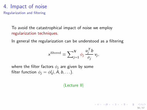
4. Impact of noiseRegularization and filtering
To avoid the catastrophical impact of noise we employregularization techniques.
In general the regularization can be understood as a filtering
xfiltered ≡∑N
j=1φj
uTj b
σjvj ,
where the filter factors φj are given by somefilter function φj = φ(j ,A, b, . . .).
〈Lecture II〉
56 / 57

Summary
� We have an discrete inverse problem which is ill-posed. Ourobservation is often corrupted by (white) noise and we wantto reconstruct the true pre-image of this observation.
� The whole concept was illustrated on the image deblurringproblem, which was closely introduced and described.
� It was shown how the problem can be reformulated as asystem of linear algebraic equations.
� We showed the typical properties of the corresponding matrixand the right-hand side, in particular the discrete Picardcondition.
� Finally, we illustrated the catastrophical impact of the noiseon the reconstruction on an example.
57 / 57