signal and image restoration: solving ill-posed inverse problems -...
TRANSCRIPT
SIGNAL AND IMAGE RESTORATION: SOLVING
ILL-POSED INVERSE PROBLEMS - ESTIMATING
PARAMETERS
Rosemary Renauthttp://math.asu.edu/˜rosie
CORNELL
MAY 10, 2013
1 / 55

Outline
BackgroundParameter EstimationSimple 1D Example Signal RestorationFeature Extraction - Gradients/Edges
Tutorial: LS SolutionStandard Analysis by the SVDImportance of the Basis and NoisePicard Condition for Ill-Posed Problems
Generalized regularizationGSVD for examining the solutionRevealing the Noise in the GSVD Basis
Applying to TV and the SB AlgorithmParameter Estimation for the TV
Conclusions and Future
2 / 55

Ill-conditioned Least Squares: Tikhonov Regularization
Solve ill-conditionedAx ≈ b
Standard Tikhonov, L approximates a derivative operator
x(λ) = arg minx{1
2‖Ax− b‖22 +
λ2
2‖Lx‖22}
x(λ) solves normal equations provided null(L)∩ null(A) = {0}
(ATA+ λ2LTL)x(λ) = ATb
This is not good for preserving edges in solutions.Not good for extracting features in images.But multiple approaches exist for estimating the parameter λ
3 / 55
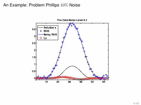
An Example: Problem Phillips 10% Noise
4 / 55

Problem Phillips 10% Noise: Tikhonov Regularized Solutions x(λ) andderivative Lx for optimal λ
Figure: Generalized Cross Validation
5 / 55

Problem Phillips 10% Noise: Tikhonov Regularized Solutions x(λ) andderivative Lx for optimal λ
Figure: L-curve
6 / 55

Problem Phillips 10% Noise: Tikhonov Regularized Solutions x(λ) andderivative Lx for optimal λ
Figure: Unbiased Predictive Risk
7 / 55

Problem Phillips 10% Noise: Tikhonov Regularized Solutions x(λ) andderivative Lx for optimal λ
Figure: Optimal χ2 - no parameter estimation!
8 / 55

An Example: Problem Shaw10% Noise
9 / 55

Problem Shaw10% Noise: Tikhonov Regularized Solutions x(λ) andderivative Lx for optimal λ
Figure: Generalized Cross Validation
10 / 55
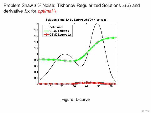
Problem Shaw10% Noise: Tikhonov Regularized Solutions x(λ) andderivative Lx for optimal λ
Figure: L-curve
11 / 55
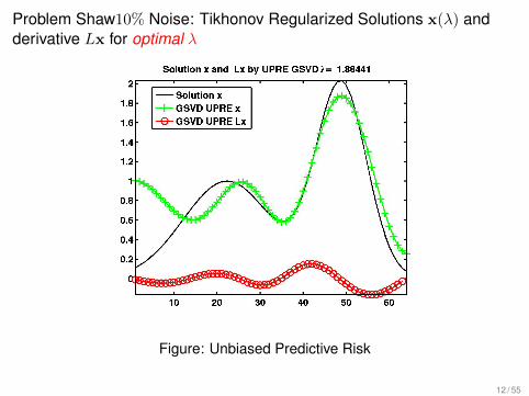
Problem Shaw10% Noise: Tikhonov Regularized Solutions x(λ) andderivative Lx for optimal λ
Figure: Unbiased Predictive Risk
12 / 55
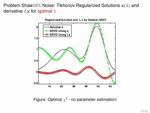
Problem Shaw10% Noise: Tikhonov Regularized Solutions x(λ) andderivative Lx for optimal λ
Figure: Optimal χ2 - no parameter estimation!
13 / 55
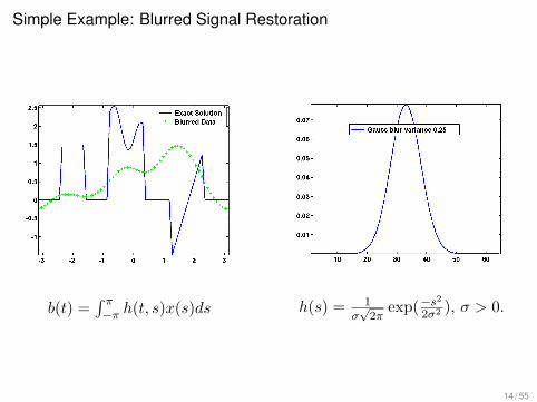
Simple Example: Blurred Signal Restoration
b(t) =∫ π−π h(t, s)x(s)ds h(s) = 1
σ√2π
exp(−s2
2σ2 ), σ > 0.
14 / 55

Example: Sample Blurred Signal 10% Noise
15 / 55

Sampled Signal 10% Noise: Tikhonov Regularized Solutions x(λ) andderivative Lx for optimal λ
Figure: Generalized Cross Validation
16 / 55

Sampled Signal 10% Noise: Tikhonov Regularized Solutions x(λ) andderivative Lx for optimal λ
Figure: L-curve
17 / 55
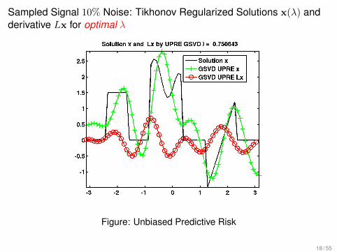
Sampled Signal 10% Noise: Tikhonov Regularized Solutions x(λ) andderivative Lx for optimal λ
Figure: Unbiased Predictive Risk
18 / 55

Sampled Signal 10% Noise: Tikhonov Regularized Solutions x(λ) andderivative Lx for optimal λ
Figure: Optimal χ2- no parameter estimation!
19 / 55

Observations
I Solutions clearly parameter dependentI For smooth signals we may be able to recover reasonable
solutionsI For non smooth signals we have a problemI Parameter estimation is more difficult for non smooth caseI What is best? What adapts for other situations?
20 / 55

Alternative Regularization: Total Variation
Consider general regularization R(x) suited to properties of x:
x(λ) = arg minx{1
2‖Ax− b‖22 +
λ2
2R(x)}
Suppose R is total variation of x (general options are possible)For example p−norm regularization p < 2
x(λ) = arg minx{‖Ax− b‖22 + λ2‖Lx‖p}
p = 1 approximates the total variation in the solution.How to solve the optimization problem for large scale?One approach - iteratively reweighted norms (Rodriguez andWohlberg) - suitable for 0 < p < 2 - depends on twoparameters.
21 / 55
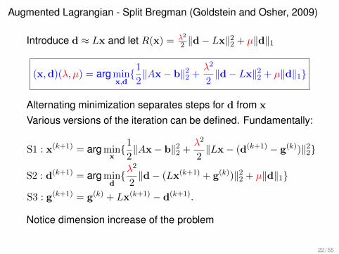
Augmented Lagrangian - Split Bregman (Goldstein and Osher, 2009)
Introduce d ≈ Lx and let R(x) = λ2
2 ‖d− Lx‖22 + µ‖d‖1
(x,d)(λ, µ) = arg minx,d{1
2‖Ax− b‖22 +
λ2
2‖d− Lx‖22 + µ‖d‖1}
Alternating minimization separates steps for d from x
Various versions of the iteration can be defined. Fundamentally:
S1 : x(k+1) = arg minx{1
2‖Ax− b‖22 +
λ2
2‖Lx− (d(k+1) − g(k))‖22}
S2 : d(k+1) = arg mind{λ
2
2‖d− (Lx(k+1) + g(k))‖22 + µ‖d‖1}
S3 : g(k+1) = g(k) + Lx(k+1) − d(k+1).
Notice dimension increase of the problem
22 / 55

Advantages of the formulation
Update for g: updates the Lagrange multiplier g
S3 : g(k+1) = g(k) + Lx(k+1) − d(k+1).
This is just - a vector updateUpdate for d:
S2 : d = arg mind{µ‖d‖1 +
λ2
2‖d− c‖22}, c = Lx + g
= arg mind{‖d‖1 +
γ
2‖d− c‖22}, γ =
λ2
µ.
This is achieved using soft thresholding.
23 / 55
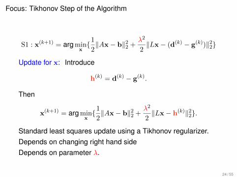
Focus: Tikhonov Step of the Algorithm
S1 : x(k+1) = arg minx{1
2‖Ax− b‖22 +
λ2
2‖Lx− (d(k) − g(k))‖22}
Update for x: Introduce
h(k) = d(k) − g(k).
Then
x(k+1) = arg minx{1
2‖Ax− b‖22 +
λ2
2‖Lx− h(k)‖22}.
Standard least squares update using a Tikhonov regularizer.Depends on changing right hand sideDepends on parameter λ.
24 / 55

The Tikhonov Update
Disadvantages of the formulationupdate for x: A Tikhonov LS update each stepChanging right hand side.Regularization parameter λ - dependent on k?Threshold parameter µ - dependent on k?
Advantages of the formulationExtensive literature on Tikhonov LS problemsTo determine stability analyze Tikhonov LS step of algorithm
I Understand the impact of the basis on the solutionI Picard conditionI Use Generalized Singular Value Decomposition for
analysis
25 / 55
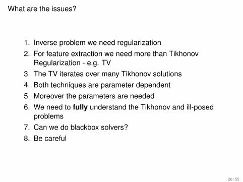
What are the issues?
1. Inverse problem we need regularization2. For feature extraction we need more than Tikhonov
Regularization - e.g. TV3. The TV iterates over many Tikhonov solutions4. Both techniques are parameter dependent5. Moreover the parameters are needed6. We need to fully understand the Tikhonov and ill-posed
problems7. Can we do blackbox solvers?8. Be careful
26 / 55

Tutorial: LS Solutions
Regularization of solution x
I SVD for the LS solutionI Basis for the LS solutionI The Picard condition
Modified RegularizationI GSVD for the regularized solutionI Changes the basisI Generalized Picard condition
27 / 55

Spectral Decomposition of the Solution: The SVD
Consider general overdetermined discrete problem
Ax = b, A ∈ Rm×n, b ∈ Rm, x ∈ Rn, m ≥ n.
Singular value decomposition (SVD) of A (full column rank)
A = UΣV T =
n∑i=1
uiσivTi , Σ = diag(σ1, . . . , σn).
gives expansion for the solution
x =n∑i=1
uTi b
σivi
ui, vi are left and right singular vectors for ASolution is a weighted linear combination of the basis vectors vi
28 / 55

The Solutions with truncated SVD- problem shaw
Figure: Truncated SVD Solutions: data enters through coefficients|uT
i b|. On the left no noise (inverse crime) in b and on the right withtiny noise 10−4
How is this impacted by the basis?
29 / 55

Some basis vectors for shaw
Figure: The first few left singular vectors vi - are they accurate?
30 / 55

Left Singular Vectors and Basis Depend on kernel (matrix A)
Figure: The first few left singular vectors ui and basis vectors vi.
Are the basis vectors accurate?
31 / 55

Use Matlab High Precision to examine the SVD
I Matlab digits allows high precision. Standard is 32.I Symbolic toolbox allows operations on high precision
variables with vpa.I SVD for vpa variables calculates the singular values
symbolically, but not the singular vectors.I Higher accuracy for the SVs generates higher accuracy
singular vectors.I Solutions with high precision can take advantage of
Matlab’s symbolic toolbox.
32 / 55

Left Singular Vectors and Basis Calculated in High Precision
Figure: The first few left singular vectors ui and basis vectors vi.Higher precision preserves the frequency content of the basis.
How many can we use in the solution for x?How does inaccurate basis impact regularized solutions?
33 / 55
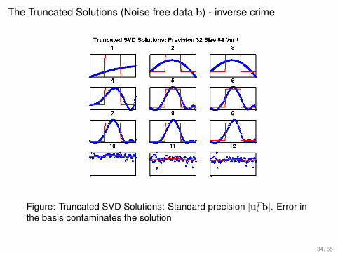
The Truncated Solutions (Noise free data b) - inverse crime
Figure: Truncated SVD Solutions: Standard precision |uTi b|. Error in
the basis contaminates the solution
34 / 55

The Truncated Solutions (Noise free data b) - inverse crime
Figure: Truncated SVD Solutions: VPA calculation |uTi b|. Larger
number of accurate terms
35 / 55

Technique to detect true basis: the Power Spectrum for detecting whitenoise : a time series analysis technique
Suppose for a given vector y that it is a time series indexed byposition, i.e. index i.Diagnostic 1 Does the histogram of entries of y generate
histogram consistent with y ∼ N(0, 1)? (i.e.independent normally distributed with mean 0 andvariance 1) Not practical to automatically look at ahistogram and make an assessment
Diagnostic 2 Test the expectation that yi are selected from awhite noise time series. Take the Fourier transformof y and form cumulative periodogram z frompower spectrum c
cj = |(dft(y)j |2, zj =
∑ji=1 cj∑qi=1 ci
, j = 1, . . . , q,
Automatic: Test is the line (zj , j/q) close to a straight line withslope 1 and length
√5/2?
36 / 55
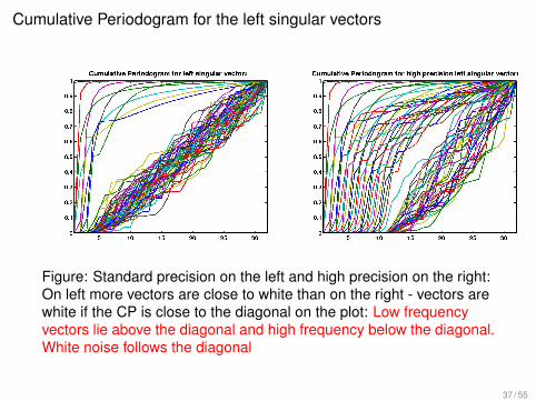
Cumulative Periodogram for the left singular vectors
Figure: Standard precision on the left and high precision on the right:On left more vectors are close to white than on the right - vectors arewhite if the CP is close to the diagonal on the plot: Low frequencyvectors lie above the diagonal and high frequency below the diagonal.White noise follows the diagonal
37 / 55
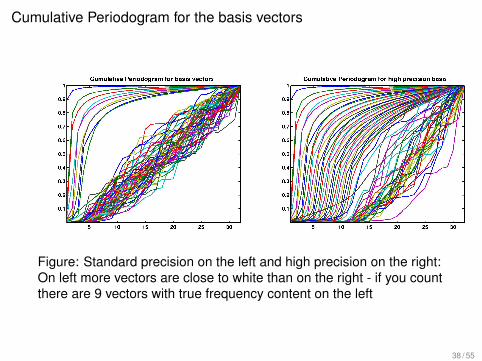
Cumulative Periodogram for the basis vectors
Figure: Standard precision on the left and high precision on the right:On left more vectors are close to white than on the right - if you countthere are 9 vectors with true frequency content on the left
38 / 55

Measure Deviation from Straight Line: Basis Vectors
Figure: Testing for white noise for the standard precision vectors:Calculate the cumulative periodogram and measure the deviationfrom the “white noise” line or assess proportion of the vector outsidethe Kolmogorov Smirnov test at a 5% confidence level for white noiselines. In this case it suggests that about 9 vectors are noise free.
Cannot expect to use more than 9 vectors in the expansion forx. Additional terms are contaminated by noise - independent ofnoise in b
39 / 55

Standard Analysis Discrete Picard condition: assesses impact of noisein the data
Recall
x =
n∑i=1
uTi b
σivi
Here|uTi b|/σi = O(1)
Ratios are not large but are the values correct? Consideringonly the discrete Picard condition does not tell us whether theexpansion for the solution is correct.
40 / 55
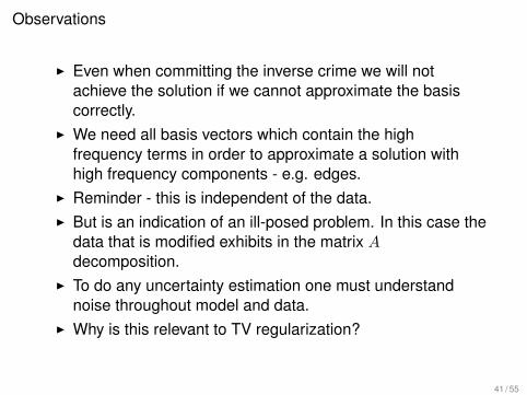
Observations
I Even when committing the inverse crime we will notachieve the solution if we cannot approximate the basiscorrectly.
I We need all basis vectors which contain the highfrequency terms in order to approximate a solution withhigh frequency components - e.g. edges.
I Reminder - this is independent of the data.I But is an indication of an ill-posed problem. In this case the
data that is modified exhibits in the matrix Adecomposition.
I To do any uncertainty estimation one must understandnoise throughout model and data.
I Why is this relevant to TV regularization?
41 / 55

Tikhonov Regularization is Spectral Filtering
xTik =
n∑i=1
φi(uTI b
σi)vi
I Tikhonov Regularization φi =σ2i
σ2i+λ
2 , i = 1 . . . n, λ is theregularization parameter, and solution is
xTik(λ) = arg minx{‖b−Ax‖2 + λ2‖x‖2}
I More general formulaton
xTik(λ) = arg minx{‖b−Ax‖2W + λ2‖Lx‖2} = arg min
x(J)
I χ2 distribution: find λ such that
E(J(x(λ))) = m+ p− n
I Yields an unregularized estimate for xI It is exactly Tikhonov regularization that is used in the SB
algorithm. But for a change of basis determined by L.42 / 55

The Generalized Singular Value Decomposition
Introduce generalization of the SVD to obtain expansion forx(λ) = arg minx{‖Ax− b‖2 + λ2‖L(x− x0)‖2}
Lemma (GSVD)Assume invertibility and m ≥ n ≥ p. There exist unitary matrices U ∈ Rm×m,V ∈ Rp×p, and a nonsingular matrix Z ∈ Rn×n such that
A = U
[Υ
0(m−n)×n
]ZT , L = V [M, 0p×(n−p)]Z
T ,
Υ = diag(υ1, . . . , υp, 1, . . . , 1) ∈ Rn×n, M = diag(µ1, . . . , µp) ∈ Rp×p,
with
0 ≤ υ1 ≤ · · · ≤ υp ≤ 1, 1 ≥ µ1 ≥ · · · ≥ µp > 0, υ2i + µ2
i = 1, i = 1, . . . p.
Use Υ̃ and M̃ to denote the rectangular matrices containing Υ and M , andnote generalized singular values: ρi = νi
µi
43 / 55

Solution of the Generalized Problem using the GSVD h = 0
x(λ) =
p∑i=1
νiν2i + λ2µ2i
(uTi b)z̃i +
n∑i=p+1
(uTi b)z̃i
z̃i is the ith column of (ZT )−1.Equivalently with filter factor φi
x(λ) =
p∑i=1
φiuTi b
νiz̃i +
n∑i=p+1
(uTi b)z̃i,
Lx(λ) =
p∑i=1
φiuTi b
ρivi, φi =
ρ2iρ2i + λ2
,
44 / 55
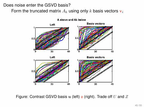
Does noise enter the GSVD basis?Form the truncated matrix Ak using only k basis vectors vi
Figure: Contrast GSVD basis u (left) z (right). Trade off U and Z
45 / 55

The TIK update of the TV algorithm
Update for x: using the GSVD : basis Z
x(k+1) =
p∑i=1
(νiu
Ti b
ν2i + λ2µ2i+λ2µiv
Ti h
(k)
ν2i + λ2µ2i
)zi +
n∑i=p+1
(uTi b)zi
A weighted combination of basis vectors zi: weights
(i)ν2i
ν2i + λ2µ2i
uTi b
νi(ii)
λ2µ2iν2i + λ2µ2i
vTi h(k)
µi
Notice (i) is fixed by b, but (ii) depends on the updates h(k)
i.e. (i) is iteration independentIf (i) dominates (ii) solution will converge slowly or not at allλ impacts the solution and must not over damp (ii)
46 / 55

Update of the mapped data
x(k+1) =
p∑i=1
(φi
uTi b
νi+ (1− φi)
vTi h(k)
µi
)zi +
n∑i=p+1
(uTi b)zi
Lx(k+1) =
p∑i=1
(φi
uTi b
ρi+ (1− φi)vTi h(k)
)vi.
Now the stability depends on coefficients
φiρi
1− φiφiνi
1− φiµi
with respect to the inner products uTi b, vTi h(k)
47 / 55

Examining the weights with λ increasing
Coefficients |uTi b| and |vTi h|, λ = .001, .1 and 10, k = 1, 10 and Final
48 / 55
Heuristic Observations
It is important to analyze the components of the solutionLeads to a generalized Picard condition analysis - more than Ican give hereThe basis is importantRegularization parameters should be adjusted dynamically.Theoretical results apply concerning parameter estimationWe can use χ2, UPRE etcImportant to have information on the noise levels
49 / 55

Theoretical results: using Unbiased Predictive Risk for the SB Tik
LemmaSuppose noise in h(k) is stochastic and both data fit Ax ≈ band derivative data fit Lx ≈ h are weighted by their inversecovariance matrices for normally distributed noise in b and h;then optimal choice for λ at all steps is λ = 1.
RemarkCan we expect h(k) is stochastic?
LemmaSuppose h(k+1) is regarded as deterministic, then UPREapplied to find the the optimal choice for λ at each step leads toa different optimum at each step, namely it depends on h.
RemarkBecause h changes each step the optimal choice for λ usingUPRE will change with each iteration, λ varies over all steps.
50 / 55
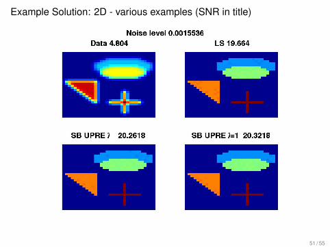
Example Solution: 2D - various examples (SNR in title)
51 / 55

Example Solution: 2D - various examples (SNR in title)
52 / 55

Example Solution: 2D - various examples (SNR in title)
53 / 55
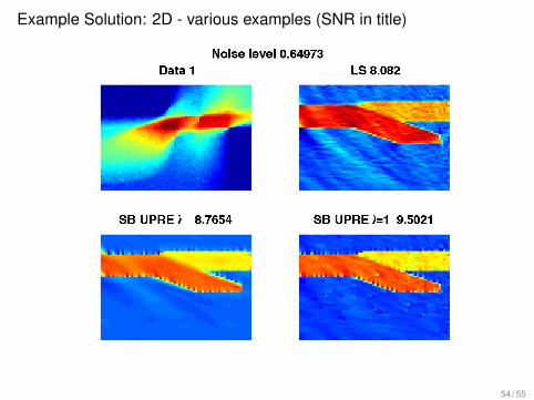
Example Solution: 2D - various examples (SNR in title)
54 / 55

Further Observations and Future Work
Results demonstrate basic analysis of problem isworthwhile
Extend standard parameter estimation from LSOverhead of optimal λ for the first step - reasonableStochastic interpretation - use fixed λ = 1 after the first
iteration is found.Practically use LSQR algorithms rather than GSVD - changes
the basis to the Krylov basis. Or use randomizedSVD to generate randomized GSVD
Noise in the basis is relevant for LSQR / CGLS iterativealgorithms
Convergence testing is based on h.
Initial work - much to do
55 / 55