image classification with deep learningranzato/files/ranzato_cnn_stanford2015.pdfimage...
TRANSCRIPT

Image Classification with Deep Learning
Marc'Aurelio Ranzato
Facebook A.I. Research
Stanford CS231A – 11 Feb. 2015www.cs.toronto.edu/~ranzato
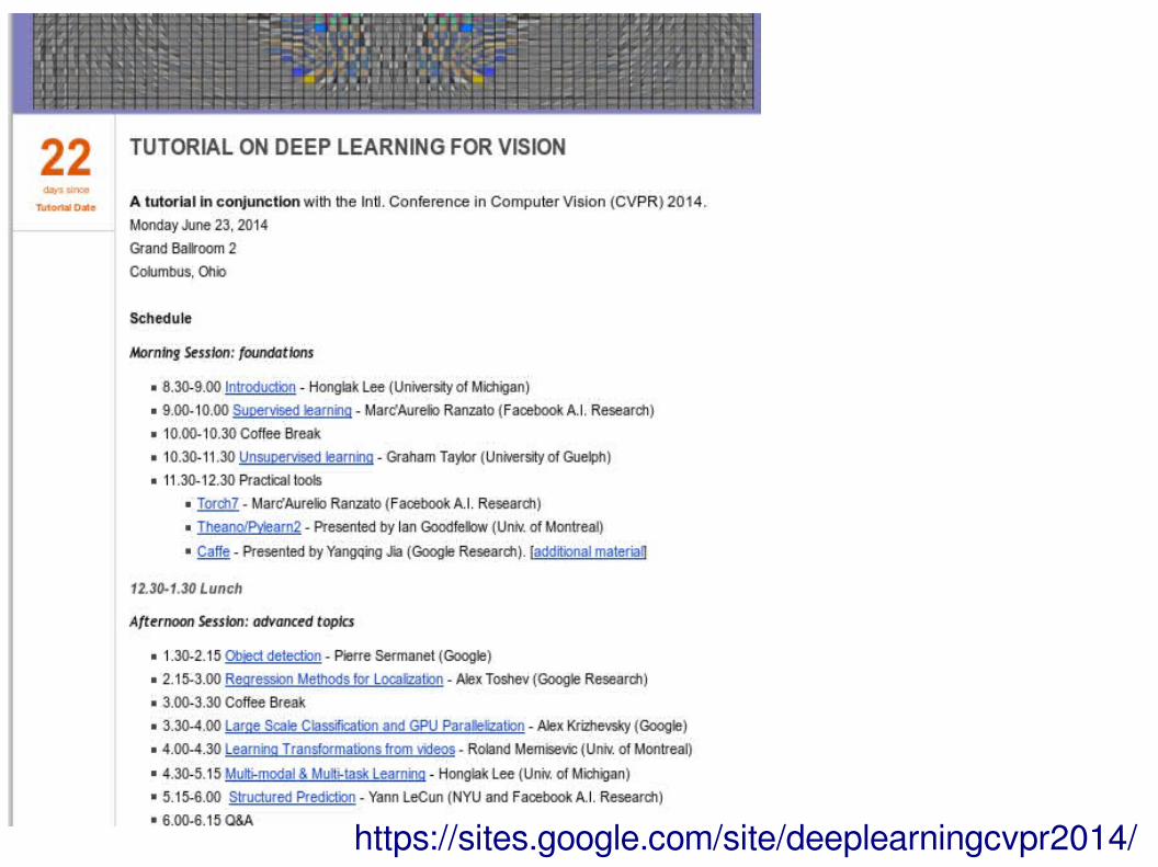
https://sites.google.com/site/deeplearningcvpr2014/
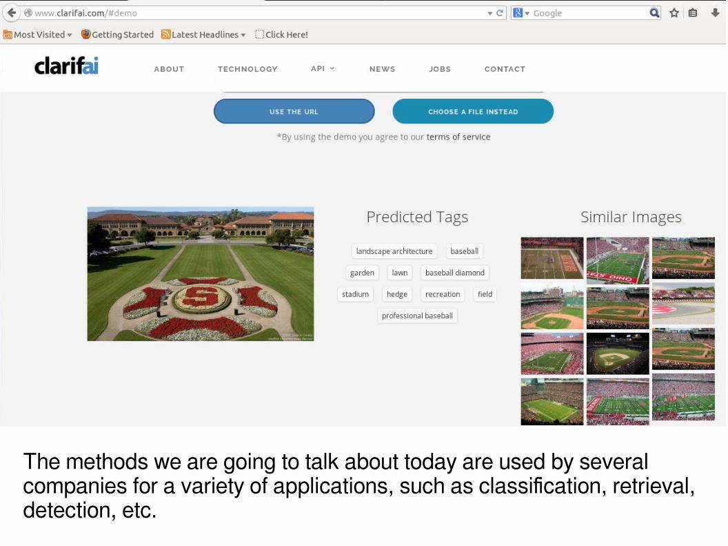
The methods we are going to talk about today are used by several companies for a variety of applications, such as classification, retrieval, detection, etc.
4
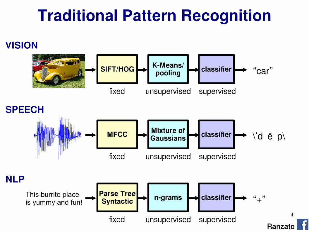
fixed unsupervised supervised
classifierMixture ofGaussiansMFCC \ˈd ē p\
fixed unsupervised supervised
classifierK-Means/poolingSIFT/HOG “car”
fixed unsupervised supervised
classifiern-gramsParse TreeSyntactic “+”This burrito place
is yummy and fun!
Traditional Pattern Recognition
VISION
SPEECH
NLP
Ranzato
5
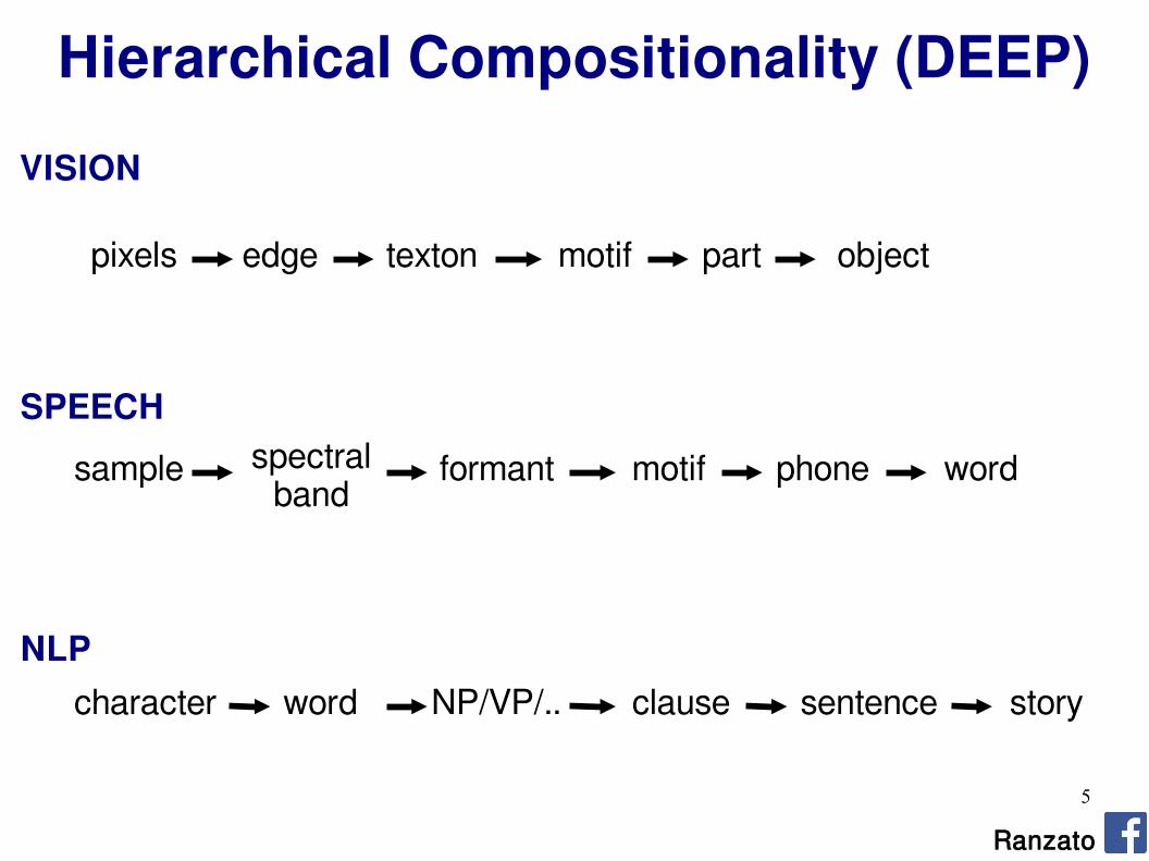
Hierarchical Compositionality (DEEP)
VISION
SPEECH
NLP
pixels edge texton motif part object
sample spectral band
formant motif phone word
character NP/VP/.. clause sentence storyword
Ranzato

6
fixed unsupervised supervised
classifierMixture ofGaussiansMFCC \ˈd ē p\
fixed unsupervised supervised
classifierK-Means/poolingSIFT/HOG “car”
fixed unsupervised supervised
classifiern-gramsParse TreeSyntactic “+”This burrito place
is yummy and fun!
Traditional Pattern Recognition
VISION
SPEECH
NLP
Ranzato
7
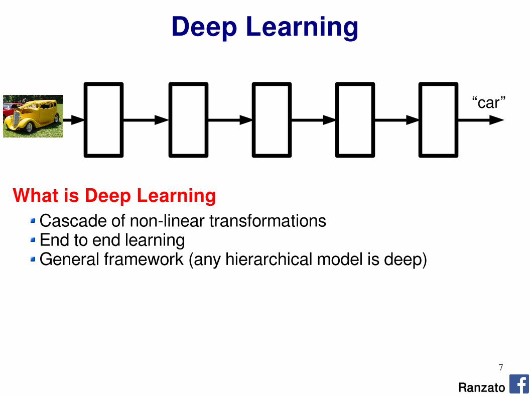
Deep Learning
“car”
Cascade of non-linear transformations End to end learning General framework (any hierarchical model is deep)
What is Deep Learning
Ranzato
8
Ranzato
THE SPACE OF MACHINE LEARNING METHODS

9
PerceptronNeural Net
Boosting
SVM
GMM
BayesNP
Convolutional Neural Net
Recurrent Neural Net
AutoencoderNeural Net
Sparse Coding
Restricted BMDeep Belief Net
Deep (sparse/denoising) Autoencoder
Disclaimer: showing only a subset of the known methods

10
PerceptronNeural Net
Boosting
SVM
GMM
BayesNP
Convolutional Neural Net
Recurrent Neural Net
AutoencoderNeural Net
Sparse Coding
Restricted BMDeep Belief Net
Deep (sparse/denoising) Autoencoder
SHA
LL
OW
DE
EP

11
PerceptronNeural Net
Boosting
SVM
GMM
BayesNP
Convolutional Neural Net
Recurrent Neural Net
AutoencoderNeural Net
Sparse Coding
Restricted BMDeep Belief Net
Deep (sparse/denoising) Autoencoder
UNSUPERVISED
SUPERVISED
DE
EP
SHA
LL
OW

12
PerceptronNeural Net
Boosting
SVM
Convolutional Neural Net
Recurrent Neural Net
AutoencoderNeural Net
Deep (sparse/denoising) Autoencoder
UNSUPERVISED
SUPERVISED
DE
EP
SHA
LL
OW
BayesNP
Deep Belief NetGMM
Sparse Coding
Restricted BM
PROBABILISTIC

13
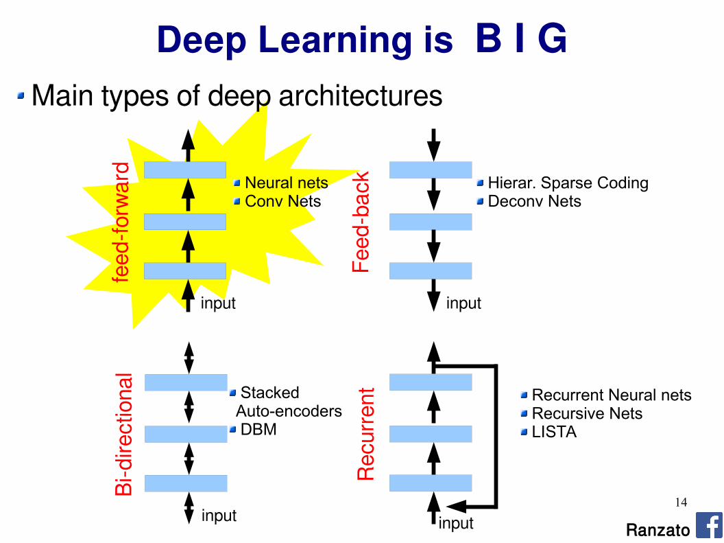
Main types of deep architectures
Ranzato
Deep Learning is B I G
input input
input
feed
-for
war
d
Feed
- bac
k
Bi-d
irect
ion a
l
Neural nets Conv Nets
Hierar. Sparse Coding Deconv Nets
Stacked Auto-encoders DBM
input
Rec
urre
nt Recurrent Neural nets Recursive Nets LISTA
14
Ranzato
Deep Learning is B I G
input input
input
feed
-for
war
d
Feed
- bac
k
Bi-d
irect
ion a
l
Neural nets Conv Nets
Hierar. Sparse Coding Deconv Nets
Stacked Auto-encoders DBM
input
Rec
urre
nt Recurrent Neural nets Recursive Nets LISTA
Main types of deep architectures
15
Ranzato
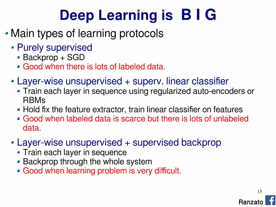
Deep Learning is B I G Main types of learning protocols
Purely supervisedBackprop + SGDGood when there is lots of labeled data.
Layer-wise unsupervised + superv. linear classifierTrain each layer in sequence using regularized auto-encoders or RBMsHold fix the feature extractor, train linear classifier on featuresGood when labeled data is scarce but there is lots of unlabeled data.
Layer-wise unsupervised + supervised backpropTrain each layer in sequenceBackprop through the whole systemGood when learning problem is very difficult.

16
Ranzato
Deep Learning is B I G Main types of learning protocols
Purely supervisedBackprop + SGDGood when there is lots of labeled data.
Layer-wise unsupervised + superv. linear classifierTrain each layer in sequence using regularized auto-encoders or RBMsHold fix the feature extractor, train linear classifier on featuresGood when labeled data is scarce but there is lots of unlabeled data.
Layer-wise unsupervised + supervised backpropTrain each layer in sequenceBackprop through the whole systemGood when learning problem is very difficult.
17
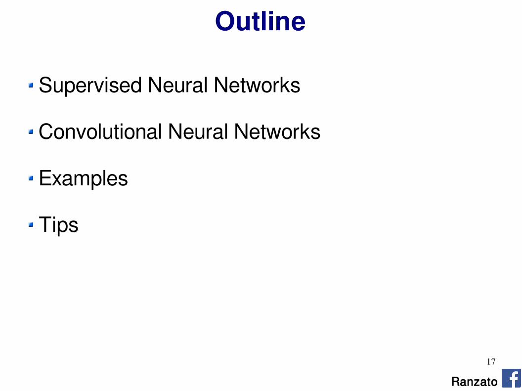
Outline
Ranzato
Supervised Neural Networks
Convolutional Neural Networks
Examples
Tips
18
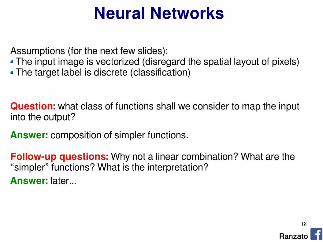
Neural Networks
Ranzato
Assumptions (for the next few slides): The input image is vectorized (disregard the spatial layout of pixels) The target label is discrete (classification)
Question: what class of functions shall we consider to map the input into the output?
Answer: composition of simpler functions.
Follow-up questions: Why not a linear combination? What are the “simpler” functions? What is the interpretation?Answer: later...
19
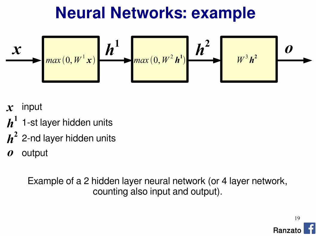
Neural Networks: example
h2h1xmax 0,W 1 x max 0,W 2 h1
W 3h2
Ranzato
input
1-st layer hidden units
2-nd layer hidden units
output
Example of a 2 hidden layer neural network (or 4 layer network, counting also input and output).
xh1
h2
o
o

20
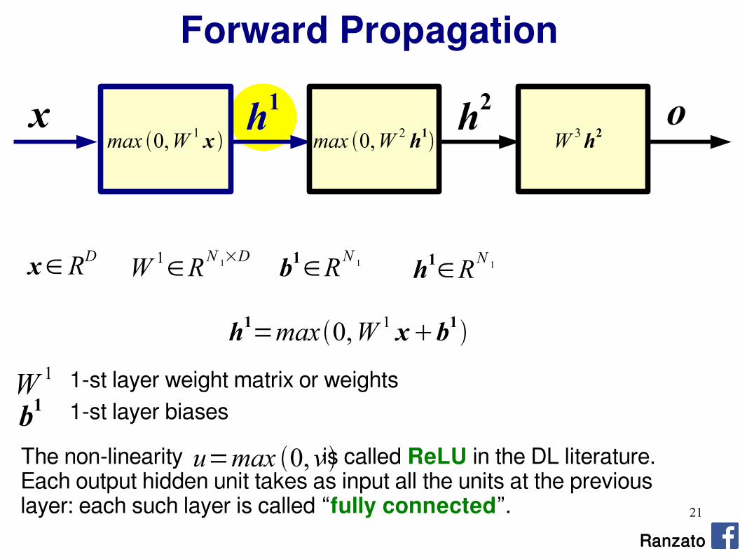
Forward Propagation
Ranzato
Def.: Forward propagation is the process of computing the output of the network given its input.
21
Forward Propagation
Ranzato
h1=max0,W 1 xb1
x∈RD W 1∈R
N 1×D b1∈R
N 1 h1∈R
N 1
x
1-st layer weight matrix or weightsW 1
1-st layer biasesb1
o
The non-linearity is called ReLU in the DL literature.Each output hidden unit takes as input all the units at the previous layer: each such layer is called “fully connected”.
u=max 0,v
h2h1
max 0,W 1 x max 0,W 2 h1 W 3h2

22
Forward Propagation
Ranzato
h2=max 0,W 2h1b2
h1∈R
N 1 W 2∈R
N 2×N 1 b2∈R
N 2 h2∈R
N 2
x o
2-nd layer weight matrix or weightsW 2
2-nd layer biasesb2
h2h1
max 0,W 1 x max 0,W 2 h1 W 3h2
23
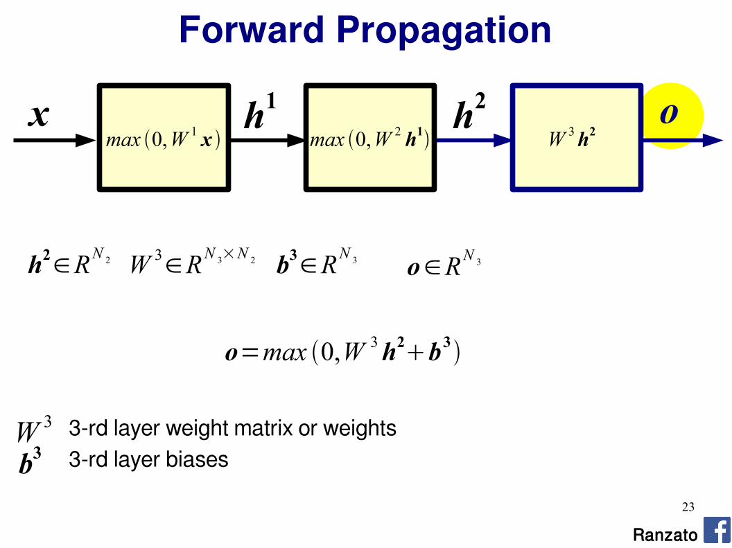
Forward Propagation
Ranzato
o=max 0,W 3h2b3
h2∈R
N 2 W 3∈R
N 3×N 2 b3∈R
N 3 o∈RN 3
x o
3-rd layer weight matrix or weightsW 3
3-rd layer biasesb3
h2h1
max 0,W 1 x max 0,W 2 h1 W 3h2
24
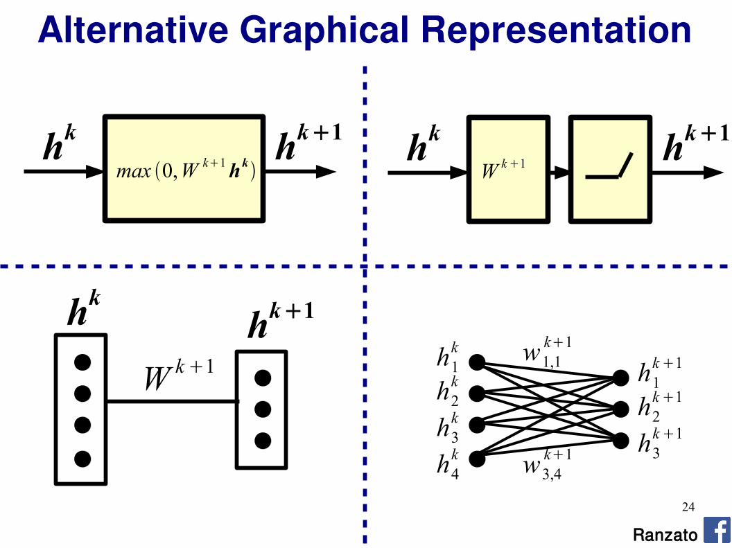
Alternative Graphical Representation
Ranzato
hk1hkmax 0,W k1hk
hk1hkW k1
h1k
h2k
h3k
h4k
h1k1
h2k1
h3k1
w1,1k1
w3,4k1
hk hk1
W k1
25
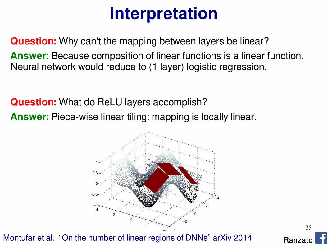
Interpretation
Ranzato
Question: Why can't the mapping between layers be linear?Answer: Because composition of linear functions is a linear function. Neural network would reduce to (1 layer) logistic regression.
Question: What do ReLU layers accomplish?Answer: Piece-wise linear tiling: mapping is locally linear.
Montufar et al. “On the number of linear regions of DNNs” arXiv 2014
26
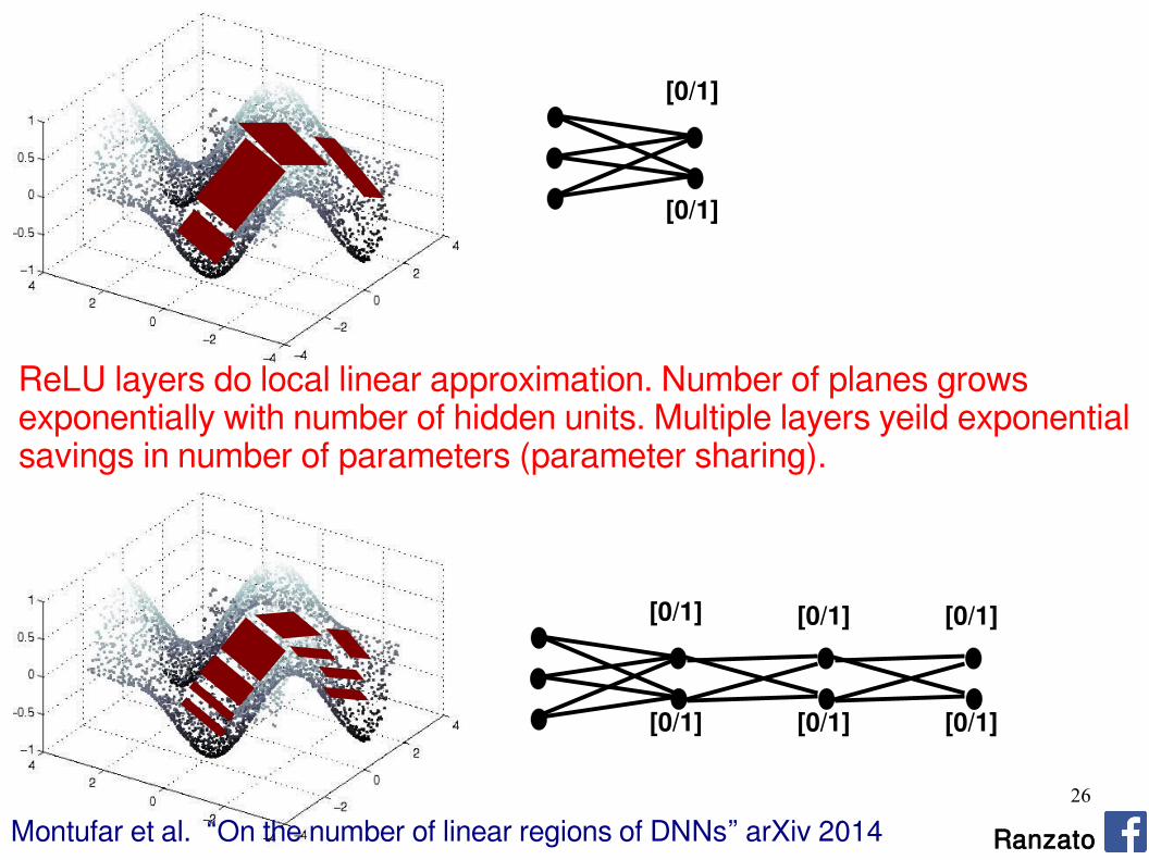
Ranzato
[0/1]
[0/1]
[0/1]
[0/1] [0/1]
[0/1]
[0/1]
[0/1]
ReLU layers do local linear approximation. Number of planes grows exponentially with number of hidden units. Multiple layers yeild exponential savings in number of parameters (parameter sharing).
Montufar et al. “On the number of linear regions of DNNs” arXiv 2014
27
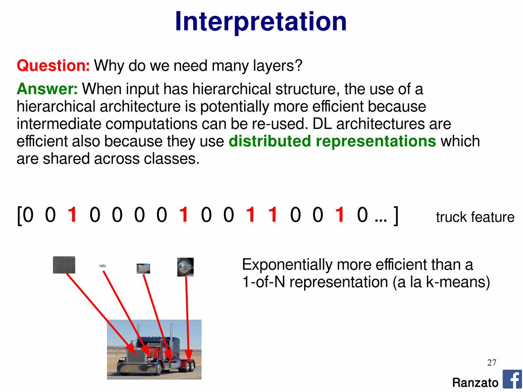
Interpretation
Ranzato
Question: Why do we need many layers?Answer: When input has hierarchical structure, the use of a hierarchical architecture is potentially more efficient because intermediate computations can be re-used. DL architectures are efficient also because they use distributed representations which are shared across classes.
[0 0 1 0 0 0 0 1 0 0 1 1 0 0 1 0 … ]
Exponentially more efficient than a 1-of-N representation (a la k-means)
truck feature
28
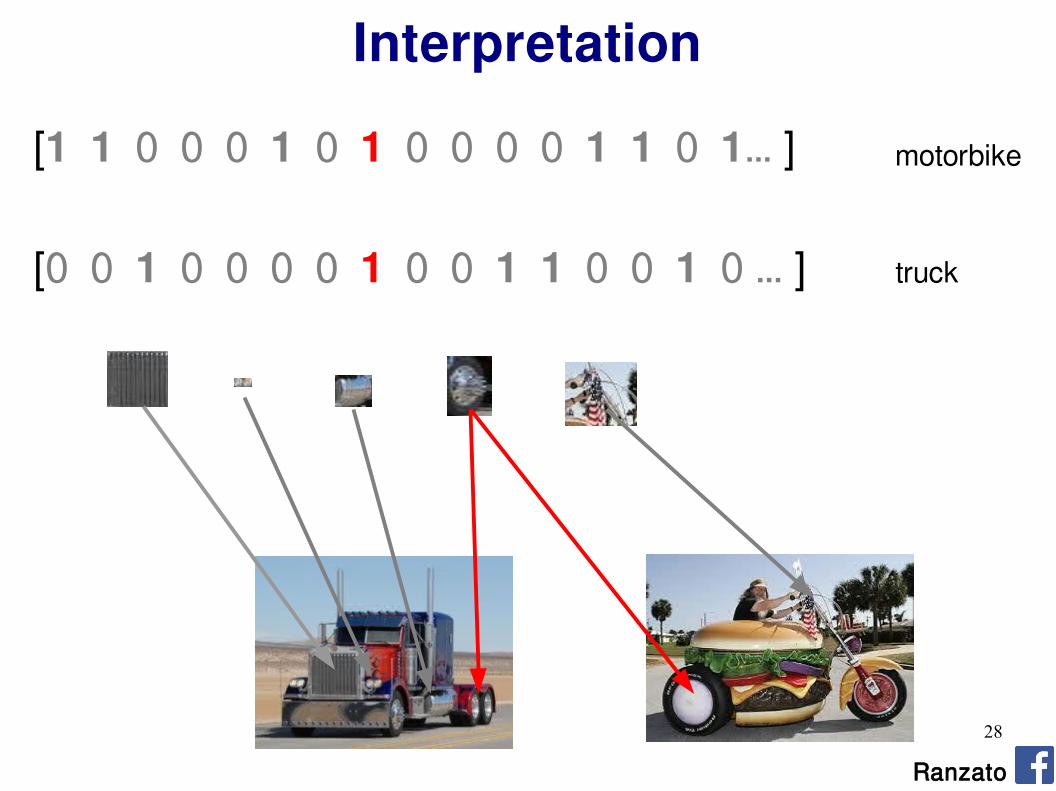
Interpretation
Ranzato
[0 0 1 0 0 0 0 1 0 0 1 1 0 0 1 0 … ]
[1 1 0 0 0 1 0 1 0 0 0 0 1 1 0 1… ] motorbike
truck

29
Interpretation
Ranzato
Input image
low level parts
prediction of class
mid-level parts
high-level parts
distributed representations feature sharing compositionality
...
Lee et al. “Convolutional DBN's ...” ICML 2009
30
Interpretation
Ranzato
Question: How many layers? How many hidden units?Answer: Cross-validation or hyper-parameter search methods are the answer. In general, the wider and the deeper the network the more complicated the mapping.
Question: What does a hidden unit do?Answer: It can be thought of as a classifier or feature detector.
Question: How do I set the weight matrices?Answer: Weight matrices and biases are learned.First, we need to define a measure of quality of the current mapping.Then, we need to define a procedure to adjust the parameters.
31
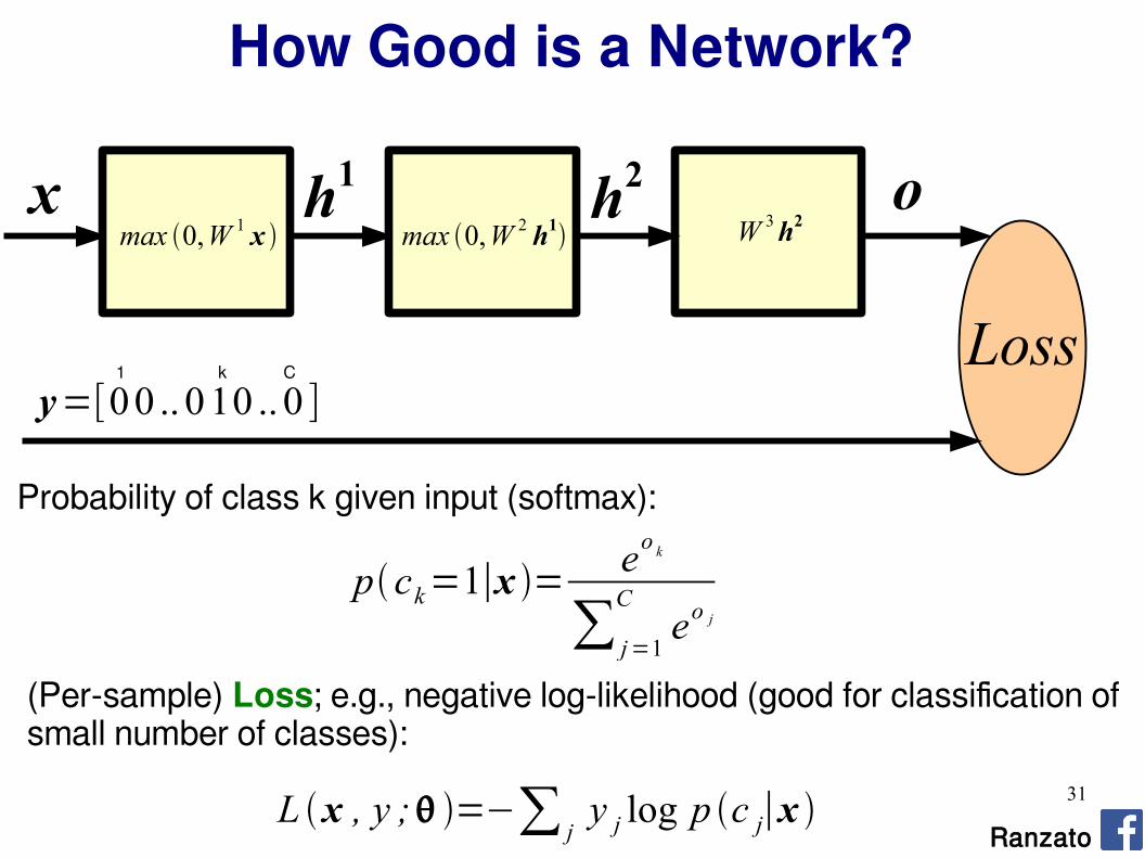
h2h1x o
Loss
max 0,W 1 x max 0,W 2 h1 W 3h2
L x , y ; =−∑ jy j log p c j∣x
pck=1∣x =eo k
∑ j=1
Ceo j
Probability of class k given input (softmax):
(Per-sample) Loss; e.g., negative log-likelihood (good for classification of small number of classes):
Ranzato
How Good is a Network?
y=[00 .. 010 .. 0 ]k1 C
32
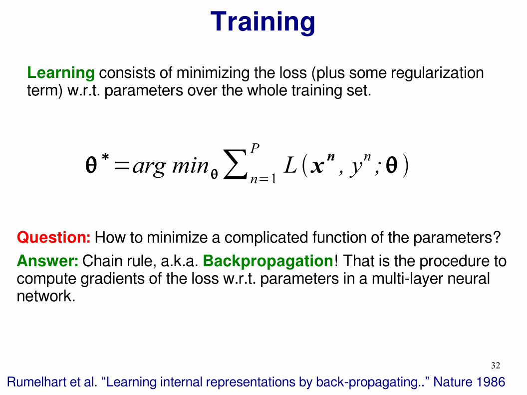
Training
∗=arg min∑n=1
PL x n , yn ;
Learning consists of minimizing the loss (plus some regularization term) w.r.t. parameters over the whole training set.
Question: How to minimize a complicated function of the parameters?Answer: Chain rule, a.k.a. Backpropagation! That is the procedure to compute gradients of the loss w.r.t. parameters in a multi-layer neural network.
Rumelhart et al. “Learning internal representations by back-propagating..” Nature 1986
33
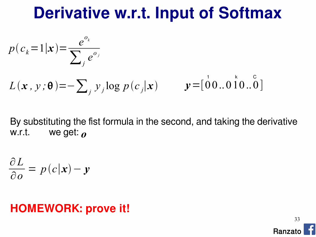
Derivative w.r.t. Input of Softmax
L x , y ; =−∑ jy j log p c j∣x
pck=1∣x =eok
∑ jeo j
By substituting the fist formula in the second, and taking the derivative w.r.t. we get: o
∂L∂o
= p c∣x− y
HOMEWORK: prove it!
Ranzato
y=[00 ..010 .. 0 ]k1 C

34
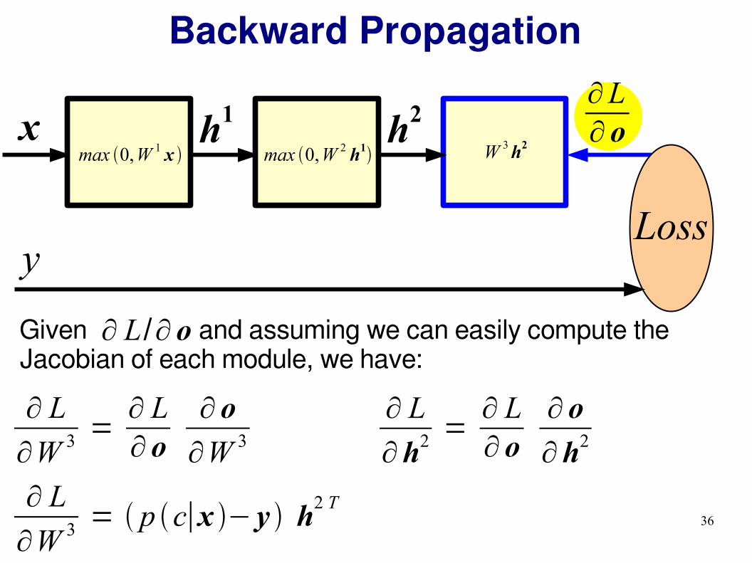
Backward Propagation
h2h1x
Lossy
Given and assuming we can easily compute the Jacobian of each module, we have:
∂ L/∂ o
∂L∂ o
max 0,W 1 x max 0,W 2 h1 W 3h2
∂ L
∂W 3 =∂ L∂ o
∂ o
∂W 3

35
Backward Propagation
h2h1x
Lossy
Given and assuming we can easily compute the Jacobian of each module, we have:
∂ L/∂ o
∂ L
∂W 3 =∂ L∂ o
∂ o
∂W 3
∂L∂ o
max 0,W 1 x max 0,W 2 h1 W 3h2
∂ L
∂W 3 = p c∣x − y h2 T
36
Backward Propagation
h2h1x
Lossy
Given and assuming we can easily compute the Jacobian of each module, we have:
∂ L/∂ o
∂ L
∂h2=
∂ L∂ o
∂ o
∂h2∂ L
∂W 3 =∂ L∂ o
∂ o
∂W 3
∂L∂ o
max 0,W 1 x max 0,W 2 h1 W 3h2
∂ L
∂W 3 = p c∣x − y h2 T

37
Backward Propagation
h2h1x
Lossy
Given and assuming we can easily compute the Jacobian of each module, we have:
∂ L/∂ o
∂ L
∂h2=
∂ L∂ o
∂ o
∂h2∂ L
∂W 3 =∂ L∂ o
∂ o
∂W 3
∂L∂ o
max 0,W 1 x max 0,W 2 h1 W 3h2
∂ L
∂W 3 = p c∣x − y h2 T ∂ L
∂h2= W
3 T pc∣x − y

38
Backward Propagation
h1x
Lossy
Given we can compute now:∂ L
∂h2
∂ L
∂h1=
∂ L
∂h2∂ h2
∂h1∂ L
∂W 2 =∂ L
∂h2∂ h2
∂W 2
∂L∂ o
∂ L
∂h2
Ranzato
max 0,W 1 x max 0,W 2 h1 W 3h2

39
Backward Propagation
x
Lossy
Given we can compute now:∂ L
∂h1
∂ L
∂W 1 =∂ L
∂h1∂ h1
∂W 1
∂ L
∂h1
Ranzato
max 0,W 1 x max 0,W 2 h1
∂L∂ o
∂ L
∂h2W 3h2

40
Backward Propagation
Ranzato
Question: Does BPROP work with ReLU layers only?Answer: Nope, any a.e. differentiable transformation works.
Question: What's the computational cost of BPROP?Answer: About twice FPROP (need to compute gradients w.r.t. input and parameters at every layer).
Note: FPROP and BPROP are dual of each other. E.g.,:
+
+
FPROP BPROP
SU
MC
OP
Y
41
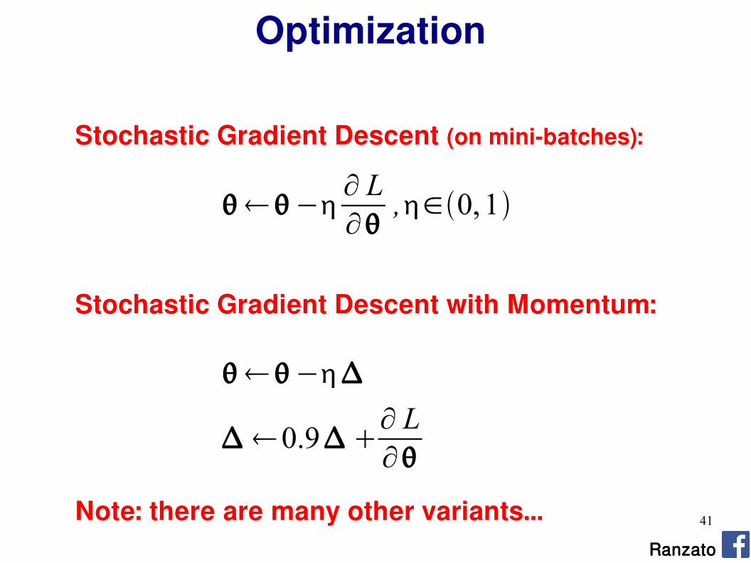
Optimization
Stochastic Gradient Descent (on mini-batches):
−∂ L∂
,∈0,1
Stochastic Gradient Descent with Momentum:
0.9 ∂ L∂
−
Ranzato
Note: there are many other variants...
42
Outline
Ranzato
Supervised Neural Networks
Convolutional Neural Networks
Examples
Tips

43
Example: 200x200 image 40K hidden units
~2B parameters!!!
- Spatial correlation is local- Waste of resources + we have not enough training samples anyway..
Fully Connected Layer
Ranzato
44
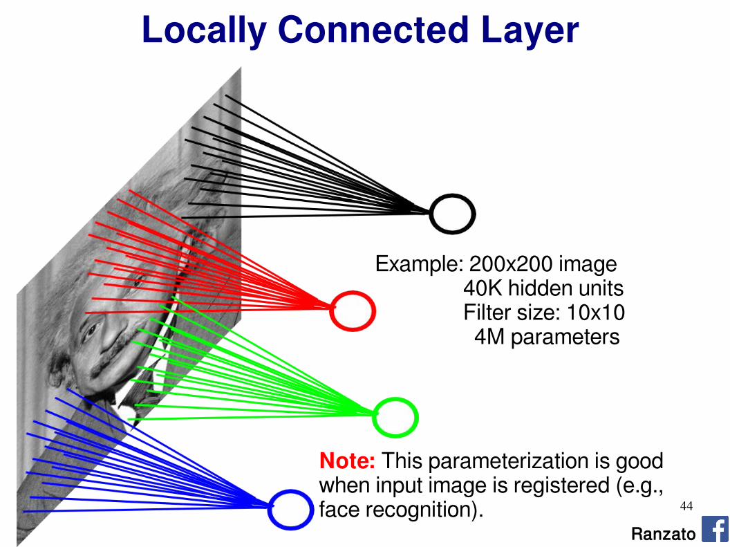
Locally Connected Layer
Example: 200x200 image 40K hidden units Filter size: 10x10
4M parameters
Ranzato
Note: This parameterization is good when input image is registered (e.g., face recognition).

45
STATIONARITY? Statistics is similar at different locations
Ranzato
Note: This parameterization is good when input image is registered (e.g., face recognition).
Locally Connected Layer
Example: 200x200 image 40K hidden units Filter size: 10x10
4M parameters

46
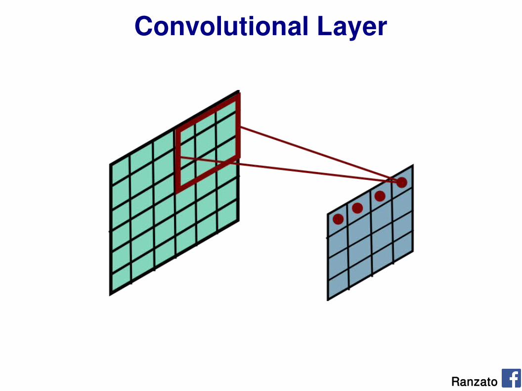
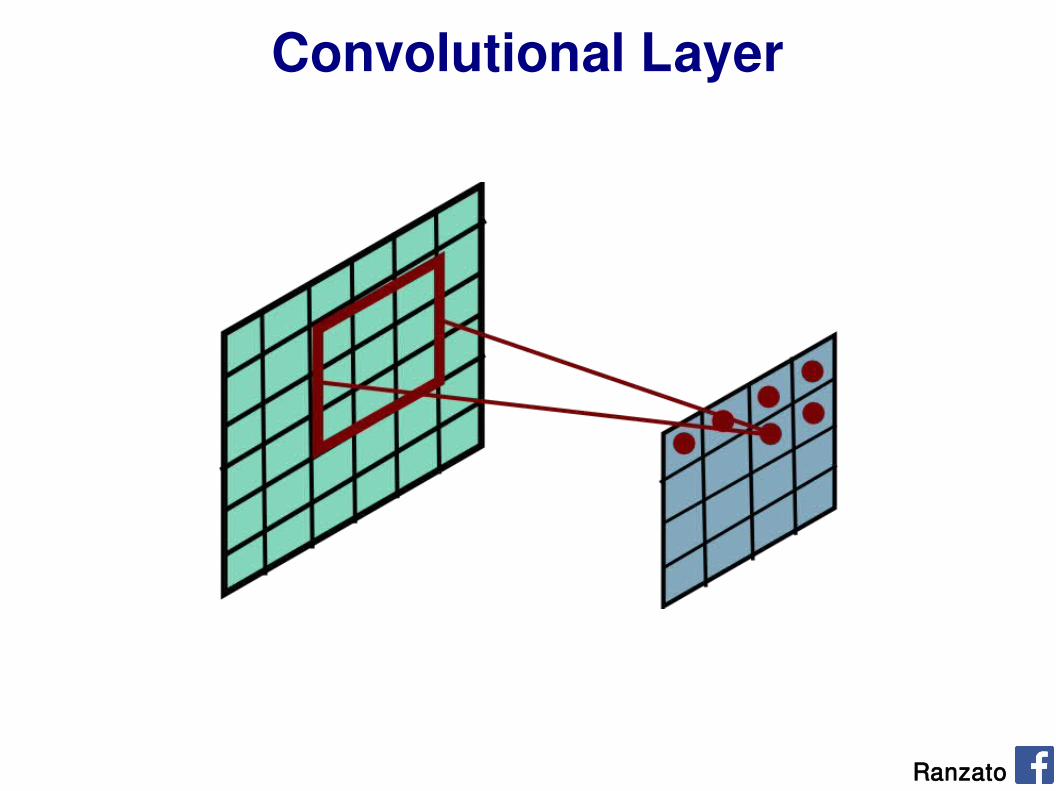
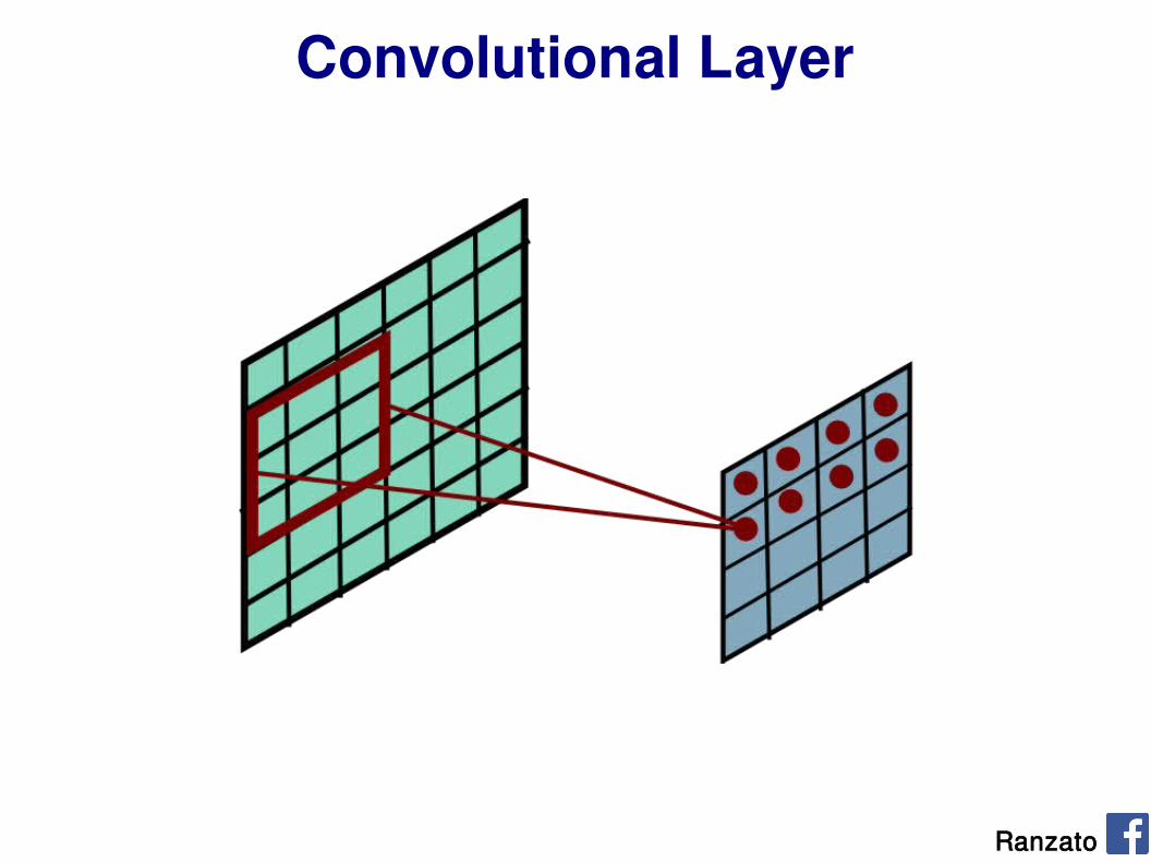
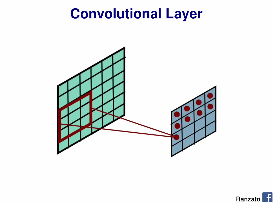
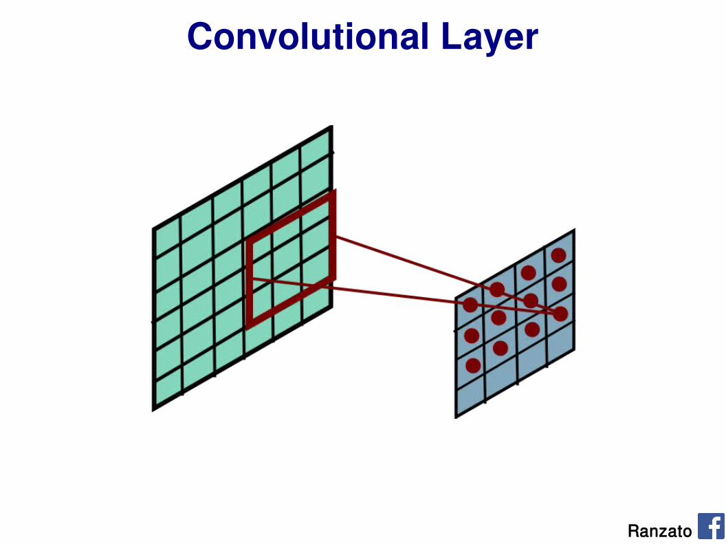
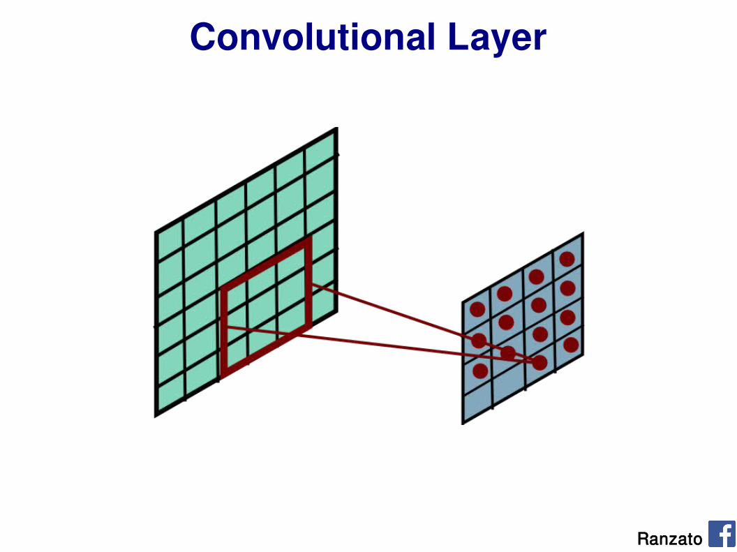
Convolutional Layer
Share the same parameters across different locations (assuming input is stationary):Convolutions with learned kernels
Ranzato

Convolutional Layer
Ranzato

Convolutional Layer
Ranzato

Convolutional Layer
Ranzato
Convolutional Layer
Ranzato

Convolutional Layer
Ranzato
Convolutional Layer
Ranzato

Convolutional Layer
Ranzato
Convolutional Layer
Ranzato
Convolutional Layer
Ranzato

Convolutional Layer
Ranzato

Convolutional Layer
Ranzato
Convolutional Layer
Ranzato

Convolutional Layer
Ranzato
Convolutional Layer
Ranzato

Convolutional Layer
Ranzato

Convolutional Layer
RanzatoMathieu et al. “Fast training of CNNs through FFTs” ICLR 2014

Convolutional Layer
*
-1 0 1-1 0 1-1 0 1
Ranzato
=

64
Learn multiple filters.
E.g.: 200x200 image 100 Filters Filter size: 10x10
10K parameters
Ranzato
Convolutional Layer

65
h jn=max 0,∑k=1
Khkn−1
∗w kjn
Ranzato
Conv.layerh1
n−1
h2n−1
h3n−1
h1n
h2n
output feature map
input feature map
kernel
Convolutional Layer

66
h jn=max 0,∑k=1
Khkn−1
∗w kjn
Ranzato
h1n−1
h2n−1
h3n−1
h1n
h2n
output feature map
input feature map
kernel
Convolutional Layer
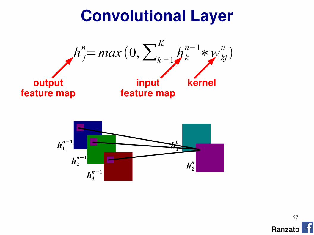
67
h jn=max 0,∑k=1
Khkn−1
∗w kjn
Ranzato
h1n−1
h2n−1
h3n−1
h1n
h2n
output feature map
input feature map
kernel
Convolutional Layer

68
Ranzato
Question: What is the size of the output? What's the computational cost?Answer: It is proportional to the number of filters and depends on the stride. If kernels have size KxK, input has size DxD, stride is 1, and there are M input feature maps and N output feature maps then:- the input has size M@DxD - the output has size N@(D-K+1)x(D-K+1)- the kernels have MxNxKxK coefficients (which have to be learned)- cost: M*K*K*N*(D-K+1)*(D-K+1)
Question: How many feature maps? What's the size of the filters?Answer: Usually, there are more output feature maps than input feature maps. Convolutional layers can increase the number of hidden units by big factors (and are expensive to compute).The size of the filters has to match the size/scale of the patterns we want to detect (task dependent).
Convolutional Layer

69
A standard neural net applied to images:- scales quadratically with the size of the input- does not leverage stationarity
Solution:- connect each hidden unit to a small patch of the input- share the weight across spaceThis is called: convolutional layer.A network with convolutional layers is called convolutional network.
LeCun et al. “Gradient-based learning applied to document recognition” IEEE 1998
Key Ideas

70
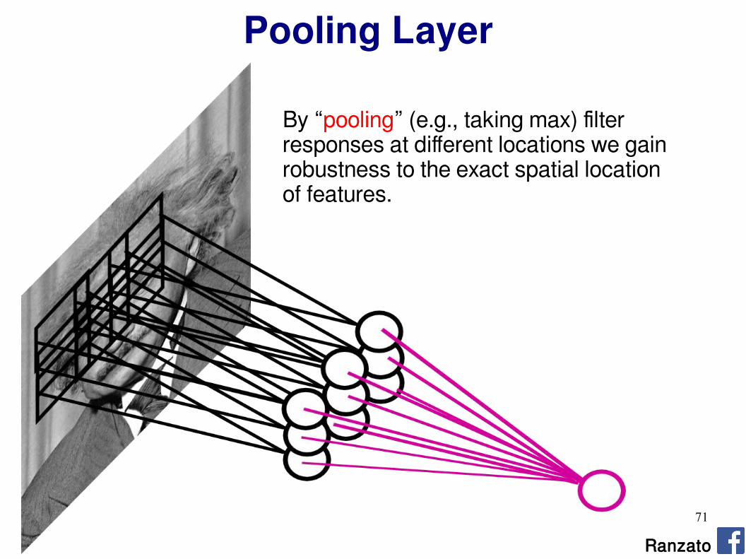
Let us assume filter is an “eye” detector.
Q.: how can we make the detection robust to the exact location of the eye?
Pooling Layer
Ranzato
71
By “pooling” (e.g., taking max) filterresponses at different locations we gainrobustness to the exact spatial locationof features.
Ranzato
Pooling Layer
72
Ranzato
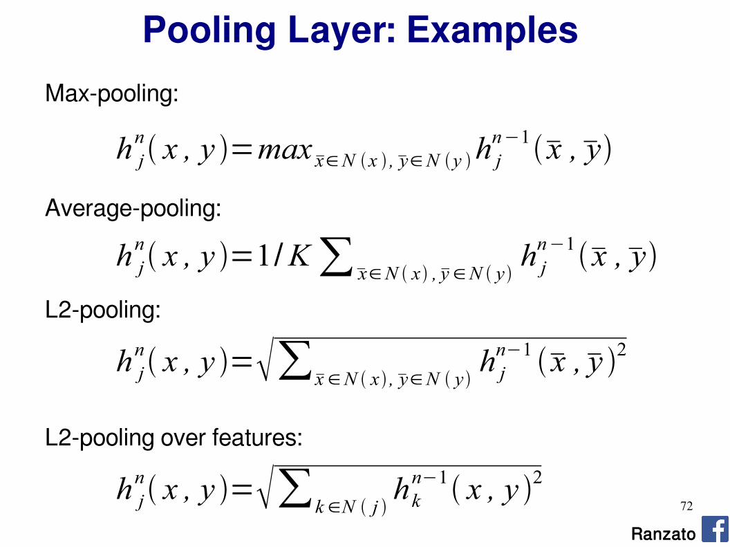
Pooling Layer: Examples
h jn x , y =max
x∈N x , y∈N y h jn−1x ,y
Max-pooling:
h jn x , y =1/K∑
x∈N x , y∈N yh jn−1
x ,y
Average-pooling:
h jn x , y =∑x∈N x , y∈N y
h jn−1 x ,y
2
L2-pooling:
h jn x , y =∑k∈N j
hkn−1 x , y 2
L2-pooling over features:
73
Ranzato
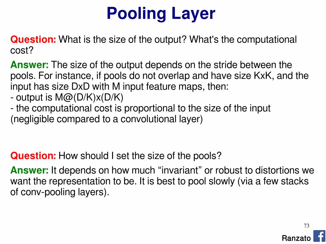
Pooling LayerQuestion: What is the size of the output? What's the computational cost?Answer: The size of the output depends on the stride between the pools. For instance, if pools do not overlap and have size KxK, and the input has size DxD with M input feature maps, then:- output is M@(D/K)x(D/K)- the computational cost is proportional to the size of the input (negligible compared to a convolutional layer)
Question: How should I set the size of the pools?Answer: It depends on how much “invariant” or robust to distortions we want the representation to be. It is best to pool slowly (via a few stacks of conv-pooling layers).
74
Ranzato
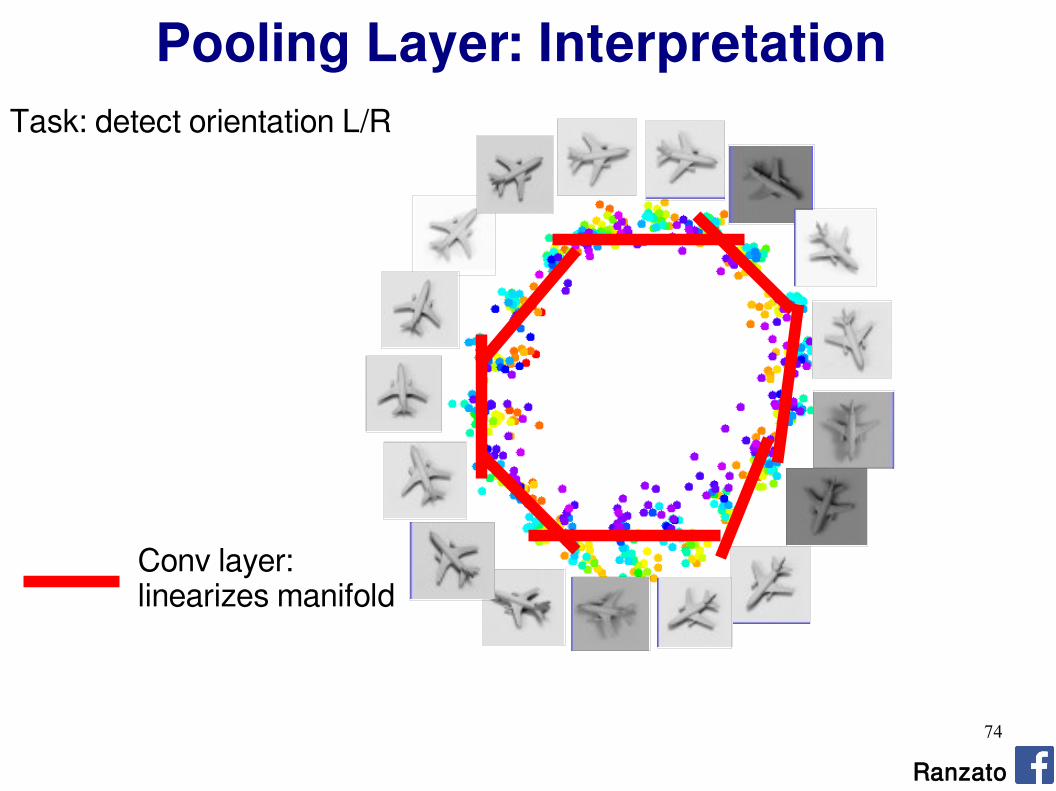
Pooling Layer: InterpretationTask: detect orientation L/R
Conv layer: linearizes manifold

75
Ranzato
Pooling Layer: Interpretation
Conv layer: linearizes manifold
Pooling layer: collapses manifold
Task: detect orientation L/R

76
Ranzato
Pooling Layer: Receptive Field Size
Conv.layer
hn−1 hn
Pool.layer
hn1
If convolutional filters have size KxK and stride 1, and pooling layer has pools of size PxP, then each unit in the pooling layer depends upon a patch (at the input of the preceding conv. layer) of size: (P+K-1)x(P+K-1)

77
Ranzato
Pooling Layer: Receptive Field Size
Conv.layer
hn−1 hn
Pool.layer
hn1
If convolutional filters have size KxK and stride 1, and pooling layer has pools of size PxP, then each unit in the pooling layer depends upon a patch (at the input of the preceding conv. layer) of size: (P+K-1)x(P+K-1)
78
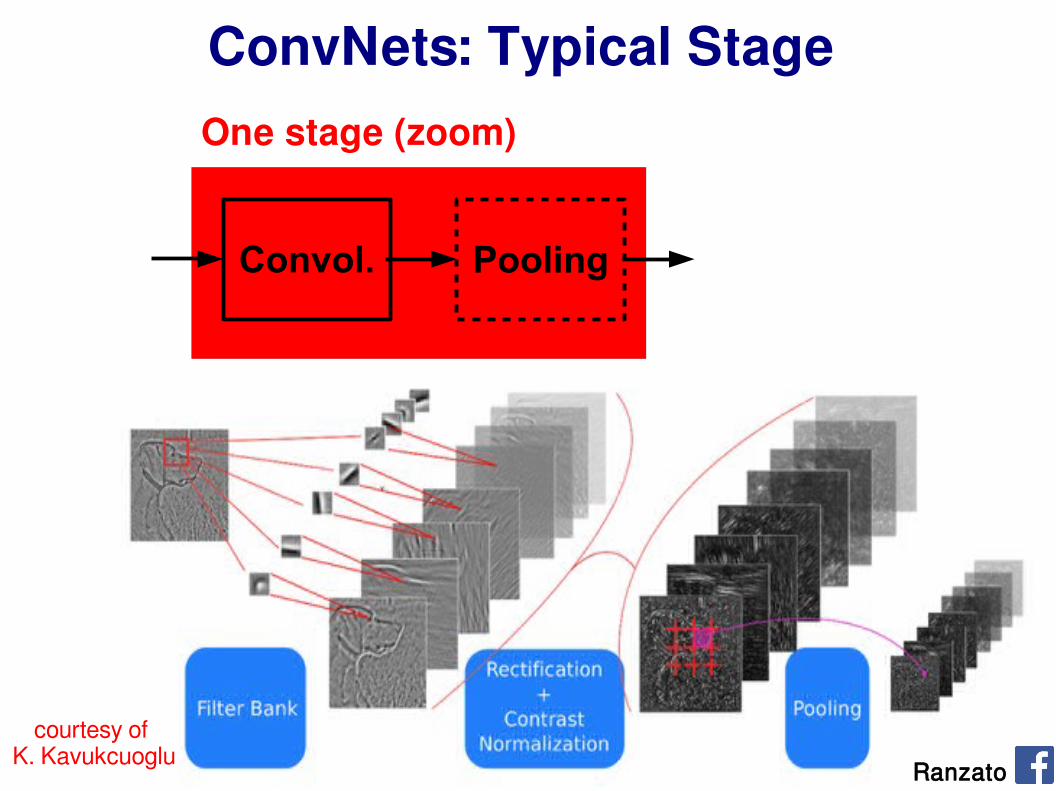
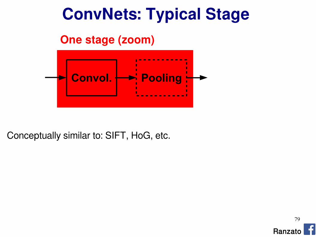
ConvNets: Typical Stage
Convol. Pooling
One stage (zoom)
courtesy of K. Kavukcuoglu Ranzato
79
One stage (zoom)
Conceptually similar to: SIFT, HoG, etc.
Ranzato
ConvNets: Typical Stage
Convol. Pooling
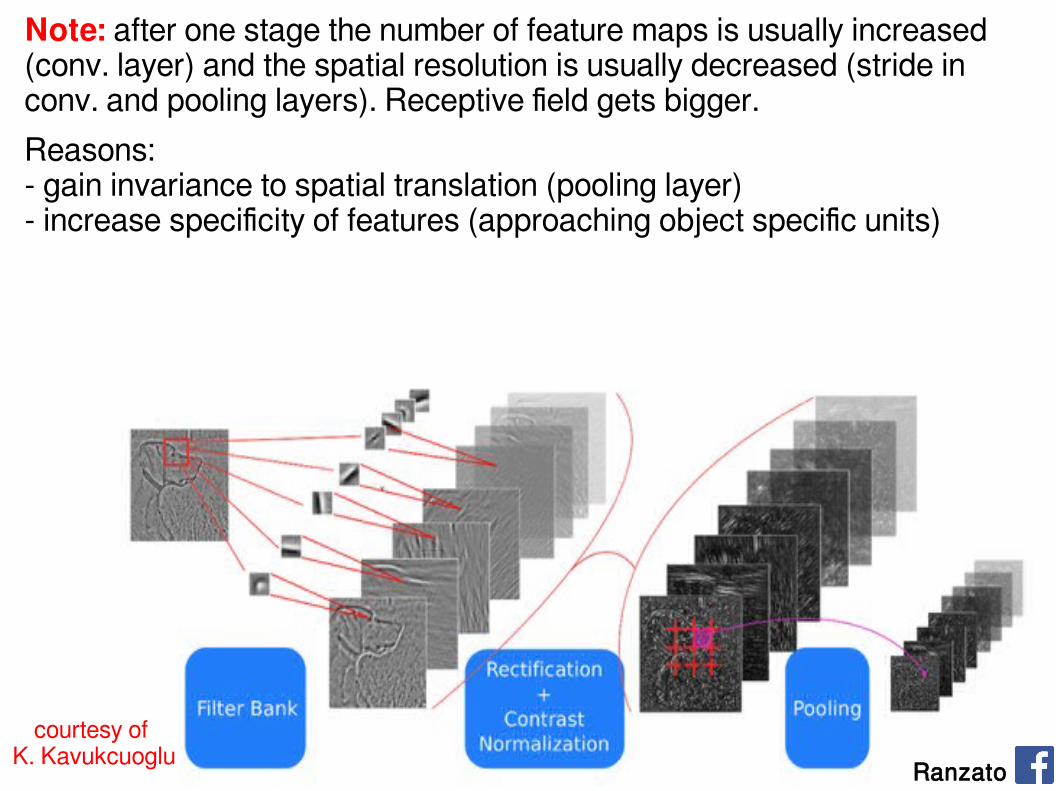
80courtesy of K. Kavukcuoglu Ranzato
Note: after one stage the number of feature maps is usually increased (conv. layer) and the spatial resolution is usually decreased (stride in conv. and pooling layers). Receptive field gets bigger.
Reasons:- gain invariance to spatial translation (pooling layer)- increase specificity of features (approaching object specific units)

81
One stage (zoom)
Fully Conn. Layers
Whole system
1st stage 2nd stage 3rd stage
Input Image
ClassLabels
Ranzato
ConvNets: Typical Architecture
Convol. Pooling

82
SIFT → K-Means → Pyramid Pooling → SVM
SIFT → Fisher Vect. → Pooling → SVM
Lazebnik et al. “...Spatial Pyramid Matching...” CVPR 2006
Sanchez et al. “Image classifcation with F.V.: Theory and practice” IJCV 2012
Conceptually similar to:
Ranzato
Fully Conn. Layers
Whole system
1st stage 2nd stage 3rd stage
Input Image
ClassLabels
ConvNets: Typical Architecture

83
ConvNets: Training
Algorithm:Given a small mini-batch- F-PROP- B-PROP- PARAMETER UPDATE
All layers are differentiable (a.e.). We can use standard back-propagation.
Ranzato
84
Ranzato
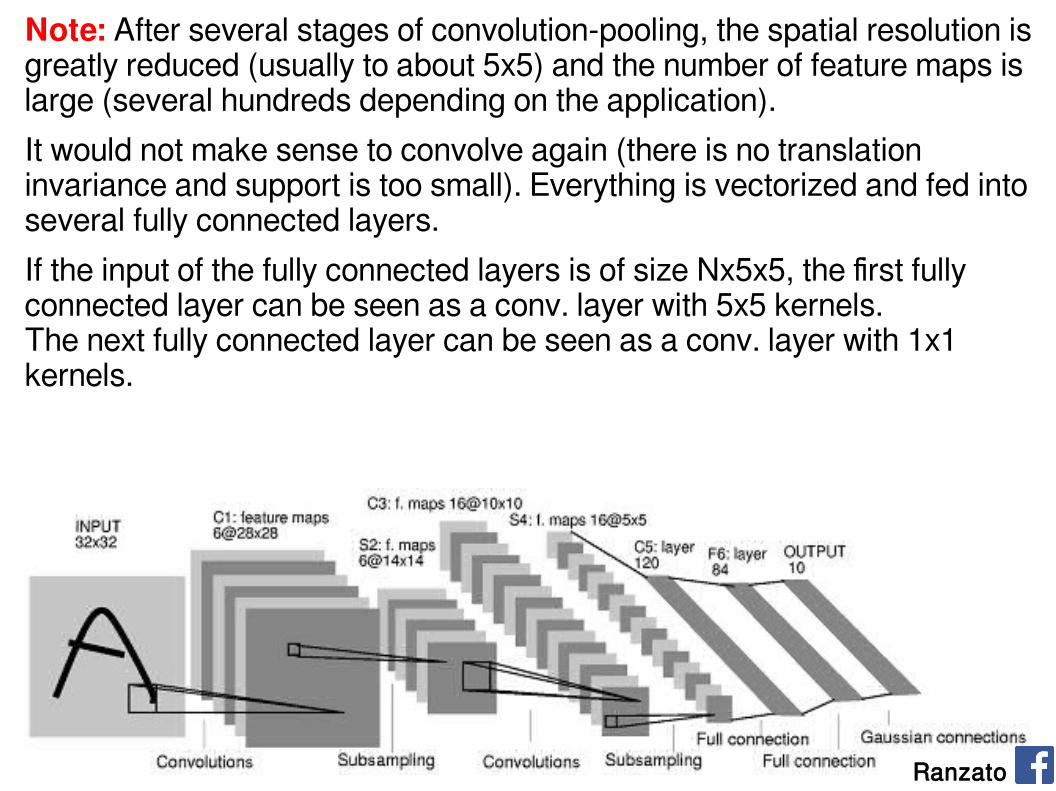
Note: After several stages of convolution-pooling, the spatial resolution is greatly reduced (usually to about 5x5) and the number of feature maps is large (several hundreds depending on the application).
It would not make sense to convolve again (there is no translation invariance and support is too small). Everything is vectorized and fed into several fully connected layers.
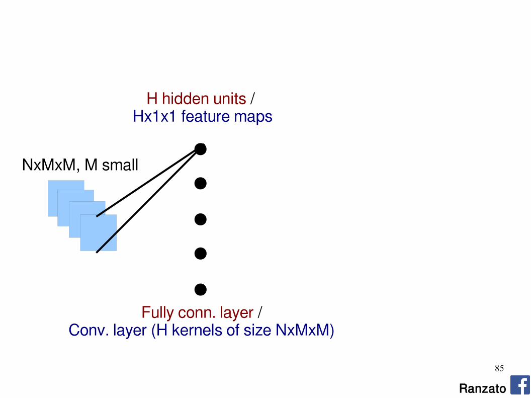
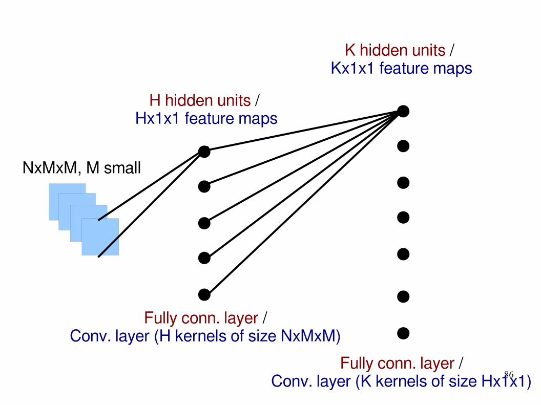
If the input of the fully connected layers is of size Nx5x5, the first fully connected layer can be seen as a conv. layer with 5x5 kernels.The next fully connected layer can be seen as a conv. layer with 1x1 kernels.
85
Ranzato
NxMxM, M small
H hidden units / Hx1x1 feature maps
Fully conn. layer /Conv. layer (H kernels of size NxMxM)
86
NxMxM, M small
H hidden units / Hx1x1 feature maps
Fully conn. layer /Conv. layer (H kernels of size NxMxM)
K hidden units / Kx1x1 feature maps
Fully conn. layer /Conv. layer (K kernels of size Hx1x1)

87
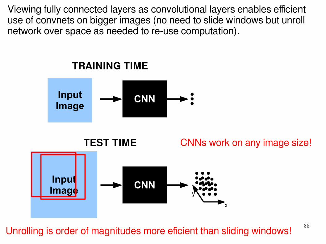
Viewing fully connected layers as convolutional layers enables efficient use of convnets on bigger images (no need to slide windows but unroll network over space as needed to re-use computation).
CNNInputImage
CNNInputImageInputImage
TRAINING TIME
TEST TIME
x
y
88
Viewing fully connected layers as convolutional layers enables efficient use of convnets on bigger images (no need to slide windows but unroll network over space as needed to re-use computation).
CNNInputImage
CNNInputImage
TRAINING TIME
TEST TIME
x
y
Unrolling is order of magnitudes more eficient than sliding windows!
CNNs work on any image size!

89
ConvNets: Test
At test time, run only is forward mode (FPROP).
Ranzato
90
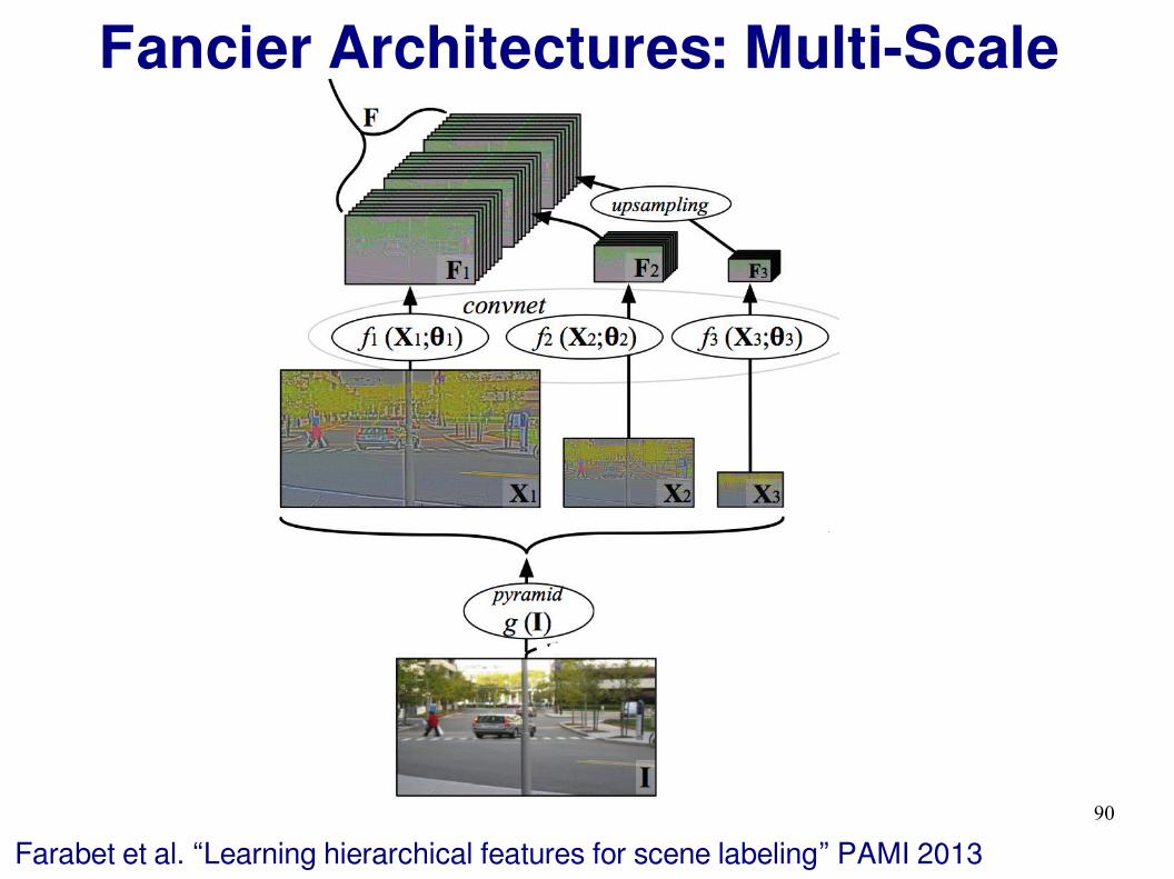
Fancier Architectures: Multi-Scale
Farabet et al. “Learning hierarchical features for scene labeling” PAMI 2013

91
Fancier Architectures: Multi-Modal
Frome et al. “Devise: a deep visual semantic embedding model” NIPS 2013
CNNText
Embedding
tiger
Matching
shared representation

92
Fancier Architectures: Multi-Task
Zhang et al. “PANDA..” CVPR 2014
ConvNormPool
ConvNormPool
ConvNormPool
ConvNormPool
FullyConn.
FullyConn.
FullyConn.
FullyConn.
...
Attr. 1
Attr. 2
Attr. N
image

93
Fancier Architectures: Multi-Task
Osadchy et al. “Synergistic face detection and pose estimation..” JMLR 2007
94
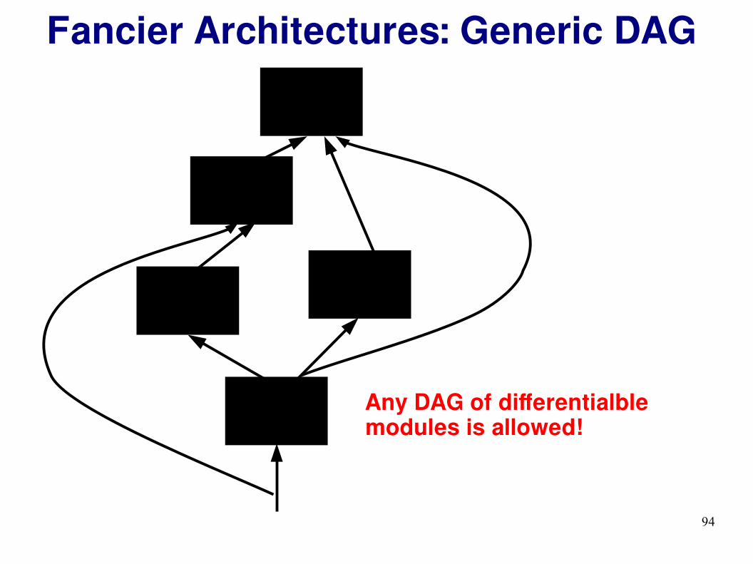
Fancier Architectures: Generic DAG
Any DAG of differentialble modules is allowed!

95
Fancier Architectures: Generic DAGIf there are cycles (RNN), one needs to un-roll it.
Graves “Offline Arabic handwriting recognition..” Springer 2012Pinheiro, Collobert “Recurrent CNN for scene labeling” ICML 2014
96
Outline
Ranzato
Supervised Neural Networks
Convolutional Neural Networks
Examples
Tips
97
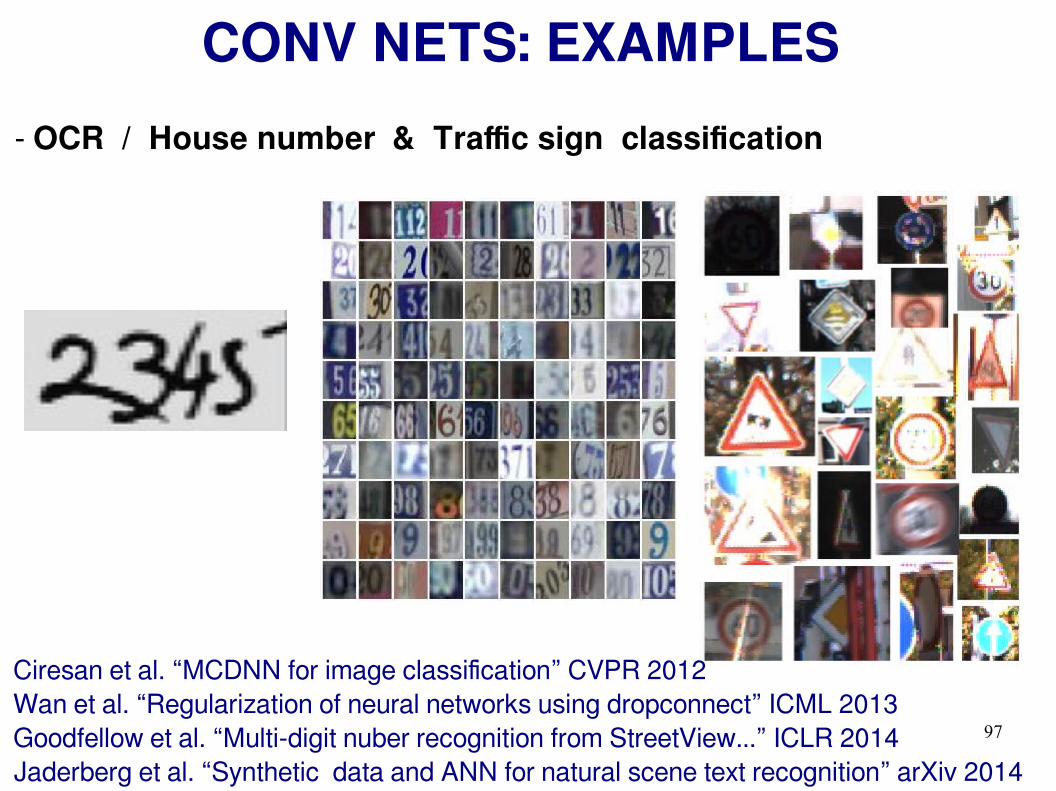
CONV NETS: EXAMPLES
- OCR / House number & Traffic sign classification
Ciresan et al. “MCDNN for image classification” CVPR 2012Wan et al. “Regularization of neural networks using dropconnect” ICML 2013Goodfellow et al. “Multi-digit nuber recognition from StreetView...” ICLR 2014Jaderberg et al. “Synthetic data and ANN for natural scene text recognition” arXiv 2014
98
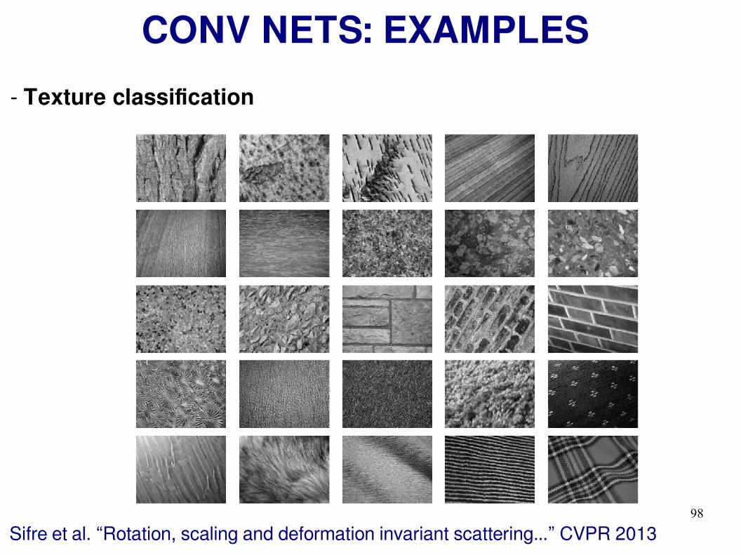
CONV NETS: EXAMPLES
- Texture classification
Sifre et al. “Rotation, scaling and deformation invariant scattering...” CVPR 2013
99
CONV NETS: EXAMPLES
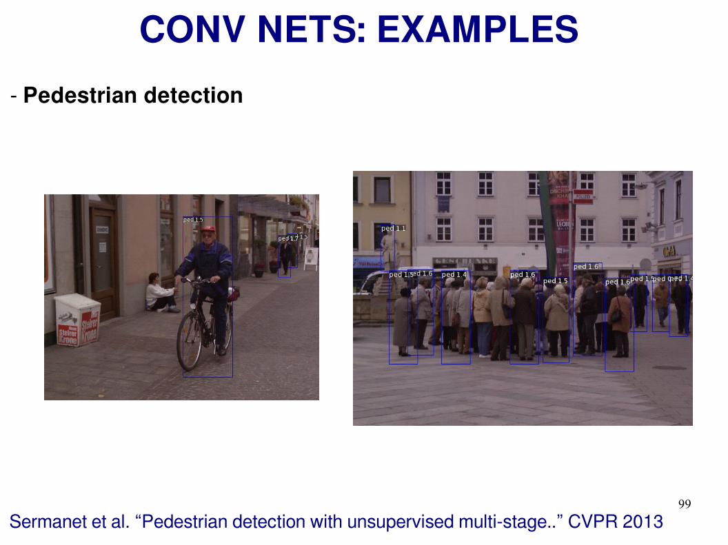
- Pedestrian detection
Sermanet et al. “Pedestrian detection with unsupervised multi-stage..” CVPR 2013

100
CONV NETS: EXAMPLES
- Scene Parsing
Farabet et al. “Learning hierarchical features for scene labeling” PAMI 2013
RanzatoPinheiro et al. “Recurrent CNN for scene parsing” arxiv 2013
101
CONV NETS: EXAMPLES
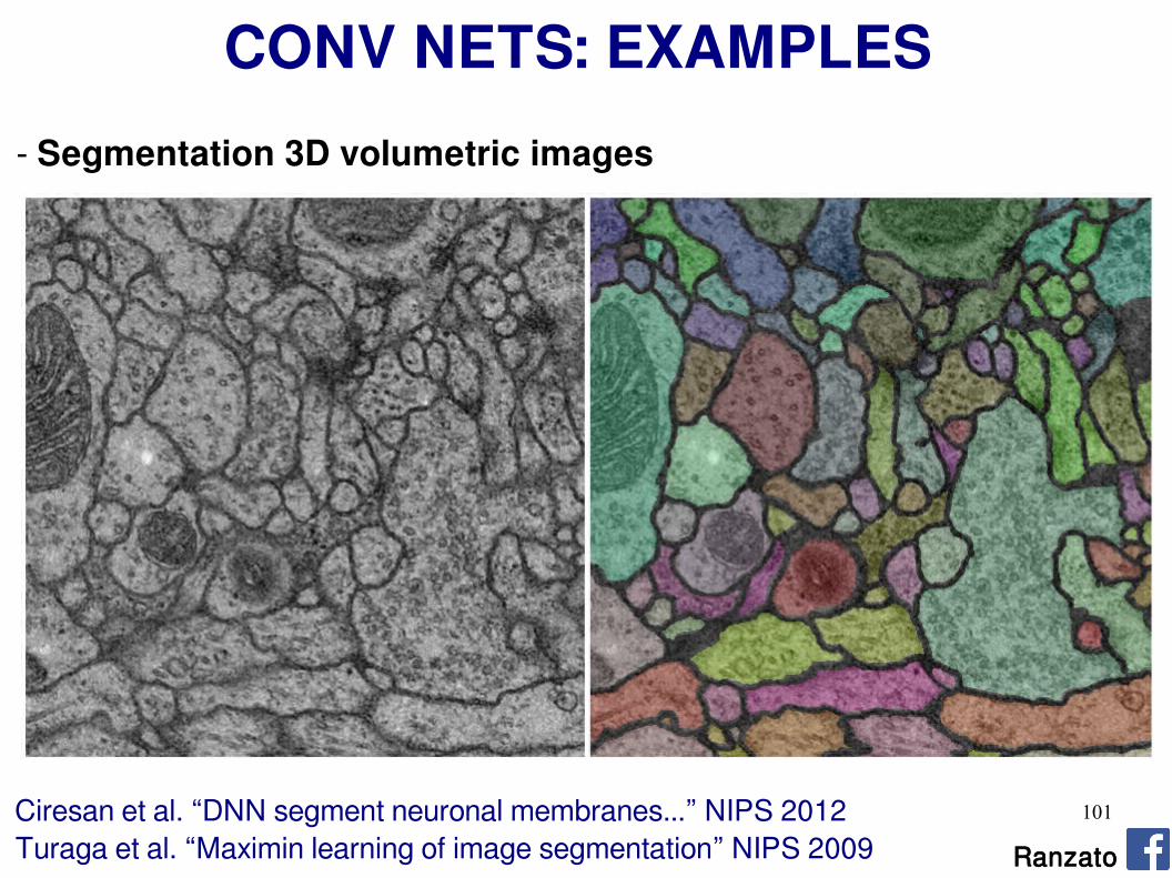
- Segmentation 3D volumetric images
Ciresan et al. “DNN segment neuronal membranes...” NIPS 2012Turaga et al. “Maximin learning of image segmentation” NIPS 2009 Ranzato
102
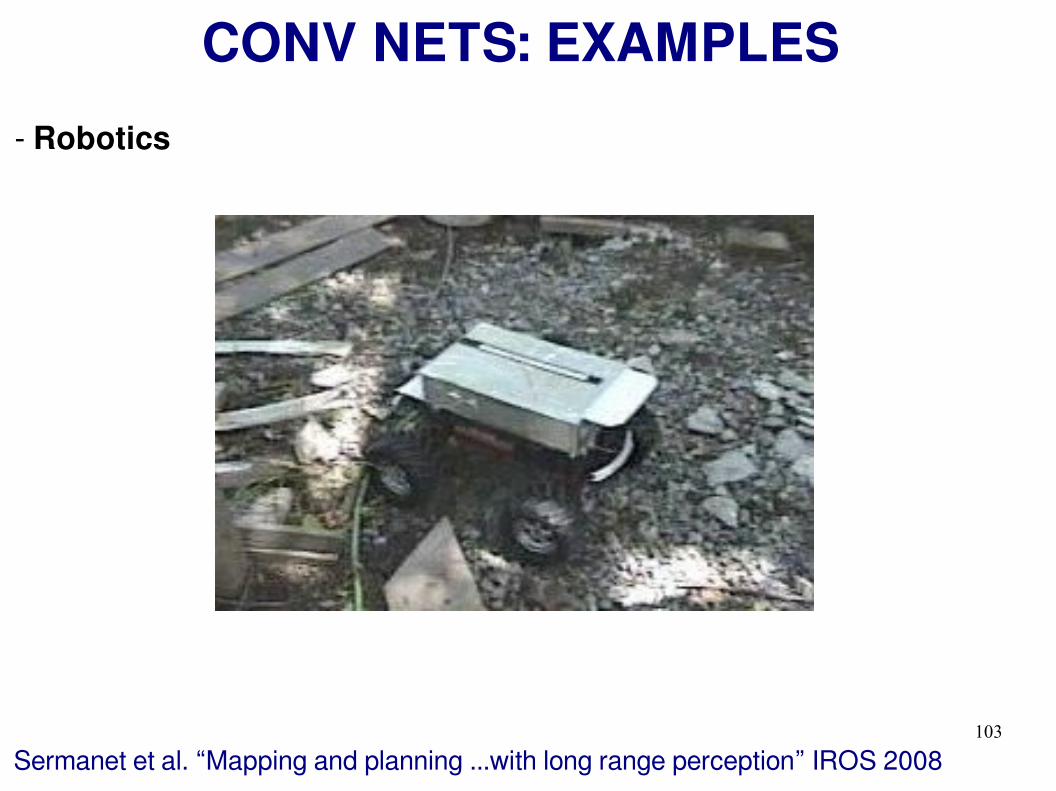
CONV NETS: EXAMPLES
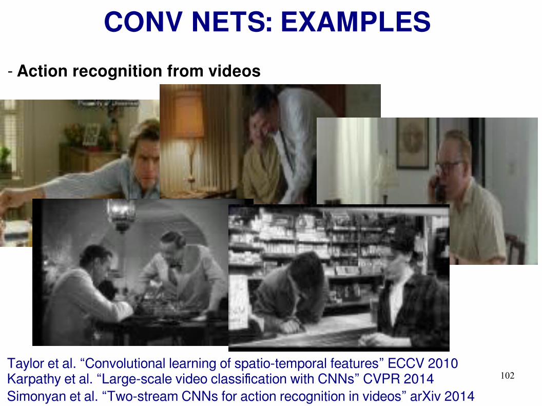
- Action recognition from videos
Taylor et al. “Convolutional learning of spatio-temporal features” ECCV 2010Karpathy et al. “Large-scale video classification with CNNs” CVPR 2014Simonyan et al. “Two-stream CNNs for action recognition in videos” arXiv 2014
103
CONV NETS: EXAMPLES
- Robotics
Sermanet et al. “Mapping and planning ...with long range perception” IROS 2008

104
CONV NETS: EXAMPLES
- Denoising
Burger et al. “Can plain NNs compete with BM3D?” CVPR 2012
original noised denoised
Ranzato
105
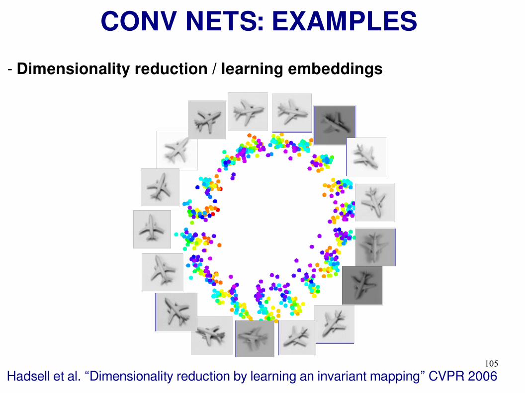
CONV NETS: EXAMPLES
- Dimensionality reduction / learning embeddings
Hadsell et al. “Dimensionality reduction by learning an invariant mapping” CVPR 2006

106
CONV NETS: EXAMPLES
- Object detection
Sermanet et al. “OverFeat: Integrated recognition, localization, ...” arxiv 2013
Szegedy et al. “DNN for object detection” NIPS 2013 RanzatoGirshick et al. “Rich feature hierarchies for accurate object detection...” arxiv 2013

Dataset: ImageNet 2012
Deng et al. “Imagenet: a large scale hierarchical image database” CVPR 2009
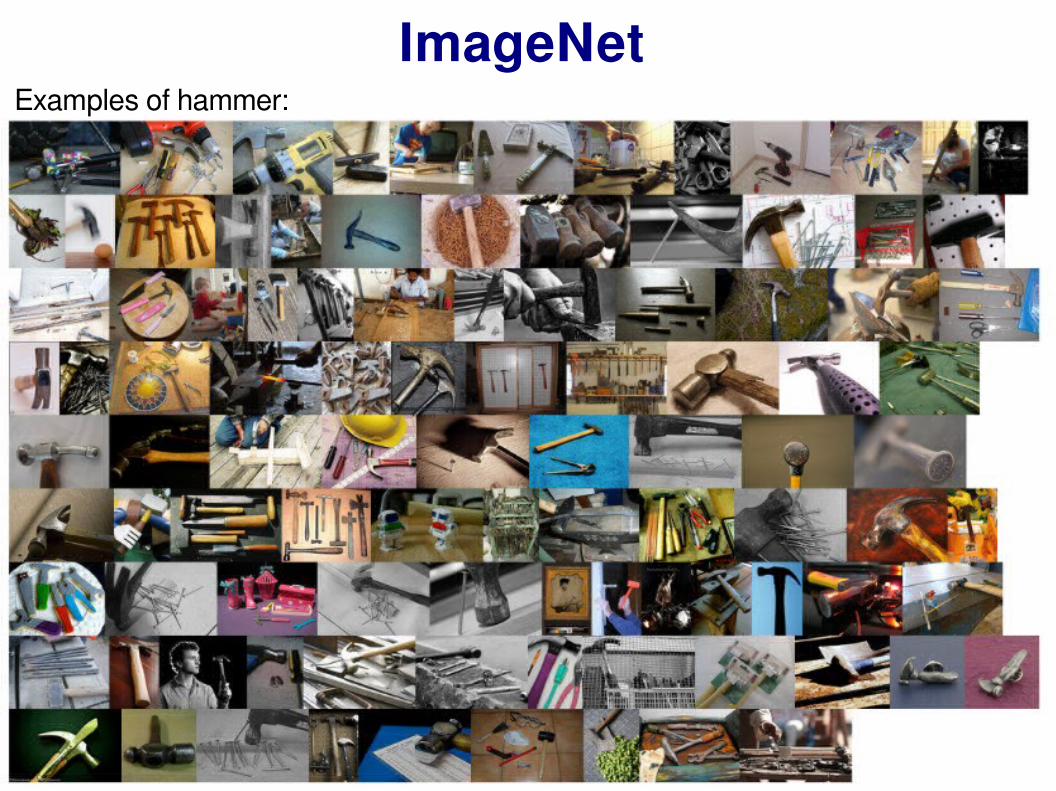
ImageNetExamples of hammer:
109
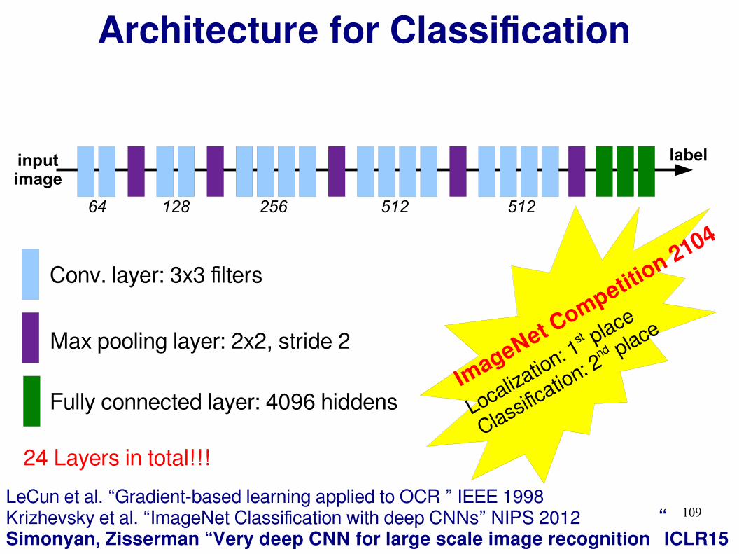
Architecture for Classification
Simonyan, Zisserman “Very deep CNN for large scale image recognition” ICLR15Krizhevsky et al. “ImageNet Classification with deep CNNs” NIPS 2012LeCun et al. “Gradient-based learning applied to OCR ” IEEE 1998
input image
label
Conv. layer: 3x3 filters
Max pooling layer: 2x2, stride 2
Fully connected layer: 4096 hiddens
64 128 256 512 512
ImageNet C
ompetition 2104
Localization: 1st place
Classification: 2nd place
24 Layers in total!!!

110
Architecture for Classification
Simonyan, Zisserman “Very deep CNN for large scale image recognition” ICLR15Krizhevsky et al. “ImageNet Classification with deep CNNs” NIPS 2012LeCun et al. “Gradient-based learning applied to OCR ” IEEE 1998
input image
label
0.1G20G
} }
FLOPS: 20G
TOTAL
111
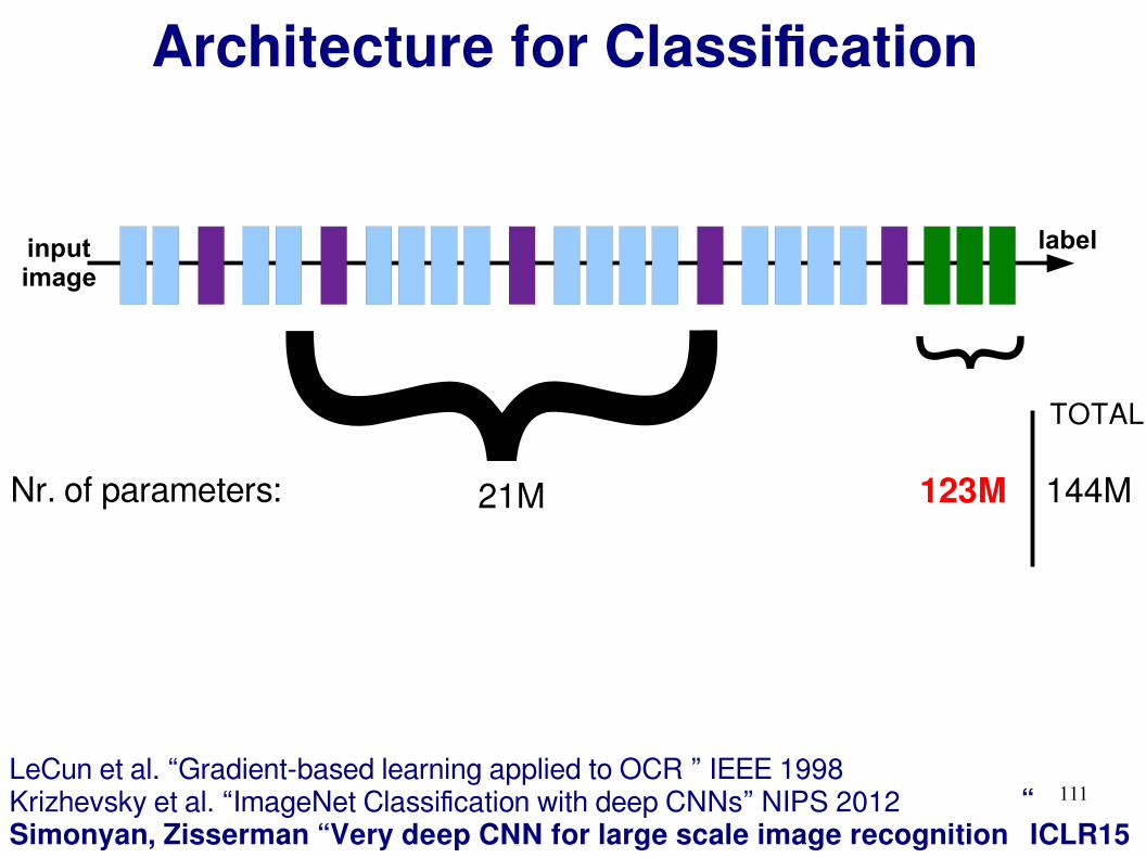
Architecture for Classification
Simonyan, Zisserman “Very deep CNN for large scale image recognition” ICLR15Krizhevsky et al. “ImageNet Classification with deep CNNs” NIPS 2012LeCun et al. “Gradient-based learning applied to OCR ” IEEE 1998
input image
label
123M21M
} }
Nr. of parameters: 144M
TOTAL
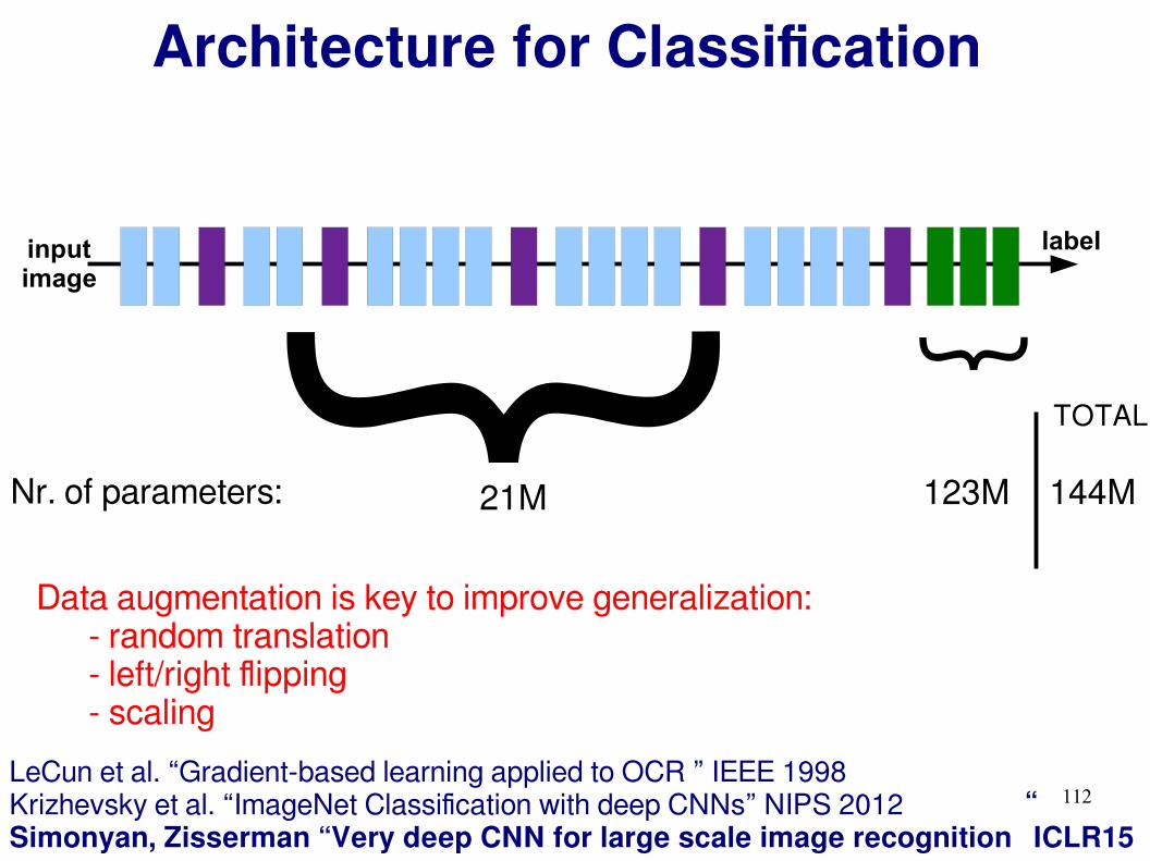
112
Architecture for Classification
Simonyan, Zisserman “Very deep CNN for large scale image recognition” ICLR15Krizhevsky et al. “ImageNet Classification with deep CNNs” NIPS 2012LeCun et al. “Gradient-based learning applied to OCR ” IEEE 1998
input image
label
123M21M
} }
Nr. of parameters: 144M
TOTAL
Data augmentation is key to improve generalization:- random translation- left/right flipping- scaling

113
Optimization
SGD with momentum: Learning rate = 0.01 Momentum = 0.9
Improving generalization by: Weight sharing (convolution) Input distortions Dropout = 0.5 Weight decay = 0.0005
Ranzato

114
Outline
Ranzato
Supervised Neural Networks
Convolutional Neural Networks
Examples
Tips
115
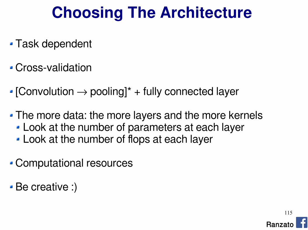
Choosing The Architecture
Task dependent
Cross-validation
[Convolution → pooling]* + fully connected layer
The more data: the more layers and the more kernelsLook at the number of parameters at each layerLook at the number of flops at each layer
Computational resources
Be creative :)
Ranzato

116
How To Optimize
SGD (with momentum) usually works very well
Pick learning rate by running on a subset of the dataBottou “Stochastic Gradient Tricks” Neural Networks 2012Start with large learning rate and divide by 2 until loss does not divergeDecay learning rate by a factor of ~1000 or more by the end of training
Use non-linearity
Initialize parameters so that each feature across layers has similar variance. Avoid units in saturation.
Ranzato
117
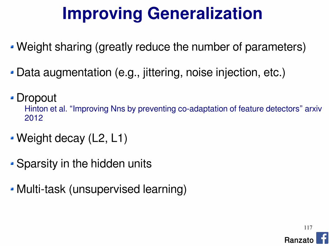
Improving Generalization
Weight sharing (greatly reduce the number of parameters)
Data augmentation (e.g., jittering, noise injection, etc.)
Dropout Hinton et al. “Improving Nns by preventing co-adaptation of feature detectors” arxiv 2012
Weight decay (L2, L1)
Sparsity in the hidden units
Multi-task (unsupervised learning)
Ranzato

118
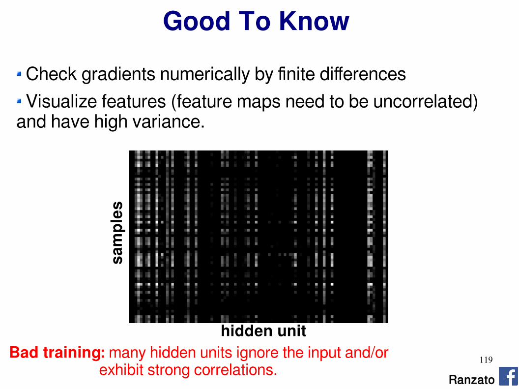
Good To Know
Check gradients numerically by finite differences Visualize features (feature maps need to be uncorrelated)
and have high variance.sa
mp
les
hidden unitGood training: hidden units are sparse across samples and across features. Ranzato
119
Check gradients numerically by finite differences Visualize features (feature maps need to be uncorrelated)
and have high variance.sa
mp
les
hidden unitBad training: many hidden units ignore the input and/or exhibit strong correlations. Ranzato
Good To Know

120
Check gradients numerically by finite differences Visualize features (feature maps need to be uncorrelated)
and have high variance. Visualize parameters
Good training: learned filters exhibit structure and are uncorrelated.
GOOD BADBAD BAD
too noisy too correlated lack structure
Ranzato
Good To Know
Zeiler, Fergus “Visualizing and understanding CNNs” arXiv 2013Simonyan, Vedaldi, Zisserman “Deep inside CNNs: visualizing image classification models..” ICLR 2014

121
Check gradients numerically by finite differences Visualize features (feature maps need to be uncorrelated)
and have high variance. Visualize parameters Measure error on both training and validation set. Test on a small subset of the data and check the error → 0.
Ranzato
Good To Know
122
What If It Does Not Work?
Training diverges:Learning rate may be too large → decrease learning rateBPROP is buggy → numerical gradient checking
Parameters collapse / loss is minimized but accuracy is low Check loss function:
Is it appropriate for the task you want to solve?Does it have degenerate solutions? Check “pull-up” term.
Network is underperformingCompute flops and nr. params. → if too small, make net largerVisualize hidden units/params → fix optmization
Network is too slowCompute flops and nr. params. → GPU,distrib. framework, make net smaller
Ranzato

123
Summary Deep Learning = learning hierarhical models. ConvNets are the
most successful example. Leverage large labeled datasets. Optimization
Plain SGD with momentum works well.
ScalingGPUsDistributed framework (Google)Better optimization techniques
Generalization on small datasets (curse of dimensionality): data augmentation weight decay dropout unsupervised learning multi-task learning
Ranzato

124
SOFTWARETorch7: learning library that supports neural net training
torch.chhttp://code.cogbits.com/wiki/doku.php (tutorial with demos by C. Farabet)https://github.com/jhjin/overfeat-torchhttps://github.com/facebook/fbcunn/tree/master/examples/imagenet
Python-based learning library (U. Montreal)
- http://deeplearning.net/software/theano/ (does automatic differentiation)
Caffe (Yangqing Jia)
– http://caffe.berkeleyvision.org
Efficient CUDA kernels for ConvNets (Krizhevsky)
– code.google.com/p/cuda-convnet
Ranzato

125
REFERENCESConvolutional Nets
– LeCun, Bottou, Bengio and Haffner: Gradient-Based Learning Applied to Document Recognition, Proceedings of the IEEE, 86(11):2278-2324, November 1998
- Krizhevsky, Sutskever, Hinton “ImageNet Classification with deep convolutional neural networks” NIPS 2012
– Jarrett, Kavukcuoglu, Ranzato, LeCun: What is the Best Multi-Stage Architecture for Object Recognition?, Proc. International Conference on Computer Vision (ICCV'09), IEEE, 2009
- Kavukcuoglu, Sermanet, Boureau, Gregor, Mathieu, LeCun: Learning Convolutional Feature Hierachies for Visual Recognition, Advances in Neural Information Processing Systems (NIPS 2010), 23, 2010
– see yann.lecun.com/exdb/publis for references on many different kinds of convnets.
– see http://www.cmap.polytechnique.fr/scattering/ for scattering networks (similar to convnets but with less learning and stronger mathematical foundations)
– see http://www.idsia.ch/~juergen/ for other references to ConvNets and LSTMs.
Ranzato

126
REFERENCESApplications of Convolutional Nets
– Farabet, Couprie, Najman, LeCun. Scene Parsing with Multiscale Feature Learning, Purity Trees, and Optimal Covers”, ICML 2012
– Pierre Sermanet, Koray Kavukcuoglu, Soumith Chintala and Yann LeCun: Pedestrian Detection with Unsupervised Multi-Stage Feature Learning, CVPR 2013
- D. Ciresan, A. Giusti, L. Gambardella, J. Schmidhuber. Deep Neural Networks Segment Neuronal Membranes in Electron Microscopy Images. NIPS 2012
- Raia Hadsell, Pierre Sermanet, Marco Scoffier, Ayse Erkan, Koray Kavackuoglu, Urs Muller and Yann LeCun. Learning Long-Range Vision for Autonomous Off-Road Driving, Journal of Field Robotics, 26(2):120-144, 2009
– Burger, Schuler, Harmeling. Image Denoisng: Can Plain Neural Networks Compete with BM3D?, CVPR 2012
– Hadsell, Chopra, LeCun. Dimensionality reduction by learning an invariant mapping, CVPR 2006
– Bergstra et al. Making a science of model search: hyperparameter optimization in hundred of dimensions for vision architectures, ICML 2013
Ranzato
127
REFERENCESLatest and Greatest Convolutional Nets
– Girshick, Donahue, Darrell, Malick. “Rich feature hierarchies for accurate object detection and semantic segmentation”, arXiv 2014
– Simonyan, Zisserman “Two-stream CNNs for action recognition in videos” arXiv 2014
- Cadieu, Hong, Yamins, Pinto, Ardila, Solomon, Majaj, DiCarlo. “DNN rival in representation of primate IT cortex for core visual object recognition”. arXiv 2014
- Erhan, Szegedy, Toshev, Anguelov “Scalable object detection using DNN” CVPR 2014
- Razavian, Azizpour, Sullivan, Carlsson “CNN features off-the-shelf: and astounding baseline for recognition” arXiv 2014
- Krizhevsky “One weird trick for parallelizing CNNs” arXiv 2014
Ranzato
128
REFERENCESDeep Learning in general
– deep learning tutorial @ CVPR 2014 https://sites.google.com/site/deeplearningcvpr2014/
– deep learning tutorial slides at ICML 2013: icml.cc/2013/?page_id=39
– Yoshua Bengio, Learning Deep Architectures for AI, Foundations and Trends in Machine Learning, 2(1), pp.1-127, 2009.
– LeCun, Chopra, Hadsell, Ranzato, Huang: A Tutorial on Energy-Based Learning, in Bakir, G. and Hofman, T. and Schölkopf, B. and Smola, A. and Taskar, B. (Eds), Predicting Structured Data, MIT Press, 2006
Ranzato
“Theory” of Deep Learning
– Mallat: Group Invariant Scattering, Comm. In Pure and Applied Math. 2012
– Pascanu, Montufar, Bengio: On the number of inference regions of DNNs with piece wise linear activations, ICLR 2014
– Pascanu, Dauphin, Ganguli, Bengio: On the saddle-point problem for non-convex optimization, arXiv 2014
- Delalleau, Bengio: Shallow vs deep Sum-Product Networks, NIPS 2011

129
THANK YOU
Ranzato